A data porting tool for coupling models withdifferent discretization needs

S.Ion∗, D.Marinescu∗, S.G.Cruceanu∗, and V.Iordache†

June 24, 2014

Abstract

The presented work is part of a larger research program dealingwith developing tools for coupling biogeochemical models in contam-inated landscapes. The specific objective of this article is to providethe researchers a tool to build hexagonal raster using information froma rectangular raster data (e.g. GIS format), data porting. This toolinvolves a computational algorithm and an open source software (writ-ten in C). The method of extending the reticulated functions definedon 2D networks is an essential key of this algorithm and can also beused for other purposes than data porting. The algorithm allows oneto build the hexagonal raster with a cell size independent from thegeometry of the rectangular raster. The extended function is a bi-cubic spline which can exactly reconstruct polynomials up to degreethree in each variable. We validate the method by analyzing errors insome theoretical case studies followed by other studies with real ter-rain elevation data. We also introduce and briefly present an iterativewater routing method and use it for validation on a case with concreteterrain data.

Keywords: Raster data, interpolation, cubic polynomials, hexagonalraster, hydrological modelling, water routing.

∗Institute of Statistical Mathematics and Applied Mathematics, Roma-nian Academy, Calea 13 Septembrie No. 13, 050711 Bucharest, Romania,Phone/Fax (4021)3182439, email: stelian.ion@ima.ro, dorin.marinescu@ima.ro,

stefan.cruceanu@ima.ro.†University of Bucharest, Research Center for Ecological Services, email:

virgil.iordache@bio.unibuc.ro

1

arX

iv:1

407.

2925

v1 [

cs.M

S] 9

Jul

201

4

1 Introduction

Predicting the long distance effects of local environmental changes requiresa coupling between local and regional models of ecological and abiotic pro-cesses. Examples include the integration of local vegetation processes withregional transport models for heavy metals (e.g. [27, 28, 29] for reviews andgeneral methodological steps), or the local resources development with move-ment of animal species (e.g. [24] for review of Partial Differential Equations(PDEs) used in spatial interactions and population dynamics, and [19] foran application using Geographic Information Systems (GIS)).

Direct coupling of the models is technically possible, but allows less flexi-bility for further model development. Alternatively, more common and flex-ible geographical objects are used as an interface among models of processesoccurring at different space-time scales. One specific problem with this inte-gration strategy is that the kind and properties of the geographical objectsused as input to or output from local and regional models are usually differ-ent (see [55] for some examples of problems raised by integrated modelling).The differences arise due to methodological constraints related to the mea-surements of the space variables and to the modelling techniques. Table 1summarizes the types of geographical objects which can occur (summarizedand developed from [18]).

It can be seen from the inspection of this table that raster data and vectordata are not basic terms in geographical ontology (see also [16]). For instancea raster refers in principle to a square tessellation of the plane with a constantvalue of the space variable function inside each square. Although raster datamodels are not a primary information source, in practical modelling they arefrequently the only available primary data source scales (e.g. in digital terrainmodels). A large volume of GIS raster data is now-a-days collected and usedfor scientific research purposes, as well as for different practical applications,and a wide variety of software has been developed over time for reading andprocessing it [23, 3] (one may also see [53] for a practical guide to use publicdomain geostatistical and GIS software). The data of a raster are organizedinto rows and columns and structured as a matrix. Any information ofinterest is characterized by an unique value in each cell which maybe “null”if no data is available. This information may represent continuous data,as elevation, temperature, rainfall intensity or discrete (thematic, nominal)data, as land use or soil category, [23]. The fidelity of a raster data withrespect to the real information is a challenging issue [11, 34, 36, 39, 48]

2

Table 1: Types of geographical objects occurring directly and indirectly in the modellingof coupled environmental process (reconstructed and adapted from [18]). Field type ap-proach allows a rigorous description of the error and empirical verification, while discretetype approach does not allow a good treatment of errors, usually involves a filtering ofempirical data.

Approach Measurement, observa-tion

Primary (“real”) geograph-ical objects

Derived (“methodologi-cal”) geographical ob-jects (resulted from datamodelling and plane dis-cretization)

Field type(propertieswith relationof spatiallocation)

Variables z - observableat a scale much smallerthan the derived ge-ographical objects andthe empirical precisionof geographical location

Variables z - observableat a scale larger than thepotentially derivable ge-ographical objects andthe empirical precisionof geographical location

Tuples < x, y, z1, . . . , zn >with space variables z andlocation (x, y).

Tuples with (x, y) on theobservation polygon or onthe transect line (e.g thecenter of the 50 x 50 mplot).

Interpolated field (the infi-nite set of tuples).

Substrates with at-tributes (polygons,contour lines, regu-larly distributed pointsas centers of a planediscretization). Thepolygons are charac-terized by a variationof the variables insidethem (a constant in thesimplest case). The sizeof the polygons is notempirically constrained;

Substrates with at-tributes. It makes nonatural sense to have thesize of the discretizationunits smaller than theobservation scale of thespatial variables.

Discrete type(substratelocated inspace withproperties)

The observation scaledoes not influence theapproach. Usually thisapproach make use ofold geographical mapsor methodological ob-jects resulted from fieldapproach.

Points, polygons, lines fill-ing and empty geographicalspace.

Field obtained by planarenforcement (points witha certain value inside thediscrete object, by class,and a constant value inthe empty space).

3

that must be taken into consideration since the errors propagate on rasterdata outputs [42, 54, 56]. Usually, large cells entail poor accuracy. Somemathematical models of environmental phenomena require information at asubgrid-scale. For example, the input data for partial differential equationsmust satisfy a certain degree of smoothness. Also, the domain discretizationmay be better suited to configurations other than that of common squarecells. Such situations may appear when one uses finite volume or finiteelement methods to numerically solve PDEs, as well as when one uses modelsbased on hexagonal cellular automata [1]. With the development of laseraltimetry in geography and ecology ([31, 50]), point clouds tend to be moreoften used for direct analysis within a GIS. Hexagonal lattices can be usedfor the extraction of knowledge by clustering techniques from such data (e.g.[30, 20]). Using the rasters obtained by interpolations of LiDAR data, [40]have pointed out the important influence of DTM resolution on the estimatedsoil loss by erosion modelling. This influence could be explored also by erosionmodels using hexagonal lattices if the porting software would be available.In this context, one can say that there is a need to build spatial interpolationalgorithms for the purpose of porting rectangular raster information to othernetworks with cells of a different size or geometry, i.e. a method of dataporting (DP). These algorithms should be developed in such a way to preserveas much as possible the original measured space variables. In this article wetackle the particular situation of variables treated by a field type approach,observable at a scale much smaller than the derived geographical objectsand the empirical precision of geographical location, having the size of thederived and not empirically constrained polygons. In particular, we presenta DP method to construct a hexagonal raster using a rectangular raster datainput. To the best of our knowledge and according to [57], there are currentlyno databases provided in “hexagonal raster format”.

1.1 Data porting methods

A rough classification divides DP into one stage and multi-stage methods.In a one stage method, the data value corresponding to a cell ci of a newgrid is given by the direct inspection of the values corresponding to the oldgrid cells that intersect ci. The methods in this class (e.g. the nearest neigh-bor, [9], area weighted mean, [57], and kriging methods, [5]) approximate thediscrete raster function. In [17], the authors develop a rescaling method alsoapplicable to the transformation of grid configuration (from rectangular to

4

triangular or hexagonal). The method is based on sampling points on theoriginal grid located around the point in the center of a pixel of the rescaledgrid. The kriging methods are well suited for irregular sample points and theyare not effective on regular and dense grids. Moreover, they require a set ofinformation concerning the correlation functions. Such information must beknown in advance or can be inferred by a proper process from the existingdata (see also [35, 10]). The multi-stage class methods [9, 32] assume theexistence of one or more intermediate (everywhere defined) functions fromwhich the cell values in the new grid are sampled. In this article, we proposea two stage method similar to one widely used in image resampling, [9, 32].The basic assumption is that the raster values represent the point valuesof an everywhere defined function that models a certain physical property.In most cases, the function is not analytically known and the raster valuesare calculated from the values of this function on a set of irregular spatiallydistributed points. The idea of constructing an intermediate stage is thatan extension function is closer than the raster to the model function. Usingthis method, the hexagonal raster tends to approximate the model functionrather than its raster representation. The construction of the intermediatefunction is essentially based on 2D bicubic interpolation. The bicubic in-terpolating polynomial is widely used in geomorphology, hydrology, imageprocessing, computer graphics, [37]. It is known that the way one choosesthe interpolating polynomial is not unique, but it strongly depends on thespecifics of the data one has to interpolate.

1.2 Applications of hexagonal raster

As an application for this hexagonal raster, we propose an iterative cel-lular automaton based method to model the drainage network of a givenlandscape. Such channel networks are of interest in domains as hydrology,geomorphology, ecology etc.

The water flow on hill slopes is a complex phenomenon that needs a lotof information concerning the physical properties about the soils and plantcover of the terrain. Focusing only on water path, one ignores all thesedetails and builds simplified models based only on the terrain topography.In this approach, the water is viewed as a thin film flowing (like rolling balls)from a cell to its adjacent neighbors. There are at least two reasons to usehexagonal instead of rectangular raster: the cell adjacency and the localsymmetry of the hexagonal structure. For the square grid case, each cell has

5

four adjacent neighbors with which shares a face and other four with whichshares a corner (all these eight neighbors forming the well known Mooreneighborhood1), and thus, some kind of anisotropy is induced by this type ofstructure. In contrast, the adjacent cells in a hexagonal raster are of the sametype, all six neighbors sharing an edge with the central cell and being at thesame distance from its center; this implies no ambiguity in defining the firstorder neighborhood of a given cell. Such kind of adjacency and the superiorsymmetry of the cells make the hexagonal raster more suitable to model waterflow, erosion, population migration etc. By example, it was observed, [8], thatflow direction vectors are better preserved for hexagonal instead of squaretilled grids when one moves from one scale to another. Moreover, concerningthe properties of symmetry, [14] showed that the mean values obtained usingsquare lattice-gas cellular automata models do not obey the Navier-Stokesequations (although the model conserves mass and momentum) due to thelack of enough symmetry, whereas hexagonal symmetry is sufficient [60]. Thisemphasizes the local group of symmetries can have major implications whenpassing from local to global level.

For regular square networks, there are many methods [41, 43, 46, 52]to extract the drainage network. All these methods assume a flow routingalgorithm and a criterion for establishing if a cell belongs to or doesn’t be-long to the discharge network. The common drawbacks of such approachesare the drainage pattern’s dependence on the grid resolution [42], the prob-lems of pits (there is no downstream flow from a cell pit) and flat regions(the flow direction cannot reliably be obtained from the neighboring cells[25, 49]) We propose here a hybrid method which combines a hexagonal flowrouting scheme with cellular automaton. Due to their simplicity, reducednumerical effort, and fast computational speed, cellular automata are cur-rently frequently used for numerical simulation of natural phenomena, see[4, 6, 13, 12, 38, 47, 58] to cite a few. Regular cellulars based on squares aredirectly compatible with GIS rasters and therefore, they are almost alwaysmet when modelling with such input data. However, there are situationswhen simulations by cellular automata on hexagonal grids are more suitablethan the ones on rectangular grids, [2, 7, 13, 44].

In Section 2 we present a general overview of DP method we are proposing

1There are situations when models with Moore type neighbors are suitable, e.g. thediscrete approximation of PDEs. On the other hand, there are physical situations wherethe boundary length between cells and a better network symmetry play an important role,and therefore this type of neighborhood is not anymore adequate.

6

in this article and we argue in its favor. After introducing some necessarynotations, we describe in Section 3 the Essentially Non-Oscillating (ENO)and Outlier Filtering (OF) algorithms used to build the 1D interpolant. Wethen present the construction of the 2D intermediate function which uses theabove 1D interpolant. The last part of this section is devoted to the process ofDP where we first describe the construction of a hexagonal network and thenpresent the numerical GIS data conversion of this network. The algorithmsaccompanying the DP method are detailed in A. Section 4 is dedicated tothe validation process of DP method and is divided into two parts. Weanalyze the errors of DP using a theoretical and then a practical datasetconsisting of terrain elevation data provided by GIS rasters. The second partof this section describes a routing method built for the hexagonal raster.The routing method is based on a simplified model of hexagonal cellularautomaton for water flow and is applied to real GIS data of some zones fromthe Romanian territory. The conclusions, perspectives and observations arepresented in the last section of this article.

2 Method

Usually, when dealing with exact interpolation by smooth functions, thereis a class of data that introduces spurious oscillations (Gibbs phenomenon,[33]). In order to eliminate this phenomenon, we propose an ENO method.ENO provides an exact and continuous interpolant for a given 1D reticu-lated function, and tries to minimize (in some sense described in Section 3.1)the oscillations produced by interpolation on the discontinuity zones of thereticulated function.

Another undesirable complication is related to the possible presence of thedata outliers. In this case, before using any interpolation method, one usuallytries to filter these outliers. In this article, we propose a direct interpolationOF method. OF eliminates the eventually rare abnormal data of a reticulatedfunction, but does not always provide an exact and continuous interpolant.

The transition from the square to a hexagonal raster data is accomplishedin four steps. First, starting from the square raster, one defines the 2Dreticulated function on the set of all square centers; its value at any suchcenter is equal to the raster datum of the square containing that center.Using this function, one then constructs the intermediate (extension) functionwhich will be defined at any point from the square raster domain. Next, one

7

defines the hexagonal cellular network, and finally constructs the hexagonalraster: the value of the hexagonal raster function on any cell will be givenby the value of the intermediate function at its center.

3 2D Bi-cubic Extension

The function extension problem is too wide a field of mathematics to betackled in a single paper, so we restrict ourselves to a narrow subject thatcan be formulated as follows. Let D be a rectangular domain in R2 and N afinite set of points (xi, yj) in D. A reticulated function is defined by

g : N → R, N =⋃i,j

(xi, yj) , g(xi, yj) = gi,j. (1)

If one thinks of the reticulated function g as a restriction to N of a functionG defined on the entire domain D, then it makes sense, when given g, toask about the values of G at a point outside of N (see [51] for an interestingdiscussion concerning the meaningfulness of spatio-temporal interpolation ofthe discrete data).

By extension of the reticulated function (1) one means a numerical schemeto estimate the value of G at any point (x, y) ∈ D. A bi-cubic extension ofthe reticulated function (1) is a function defined on the entire domain D thatis a piecewise bi-cubic polynomial function g ∈ π3,3, where π3,3 designatesthe set of all polynomials of degree three in each of the two variables x andy

g : D → R, D =⋃a

ωa, g(x, y)∣∣∣ωa∈ π3,3, (2)

with ωa the elements of a cell partition of D.The problem of the bi-cubic extension can be formulated as follows: given

a reticulated function (1), define the extension (2) that approximates themodel function G : D → R.

In what follows, we propose two methods to define a bi-cubic extension,both of them assuming a 1D extension method. The 2D extension methodis obtained by successively applying the 1D method once along the Ox andthen along the Oy directions.

To define the 1D algorithm, we need to introduce some notations. LetΞ := ξii=1,N be a set of 1D consecutive knots inside a generic interval [α, β],

8

with α ≤ ξ1 < . . . < ξN ≤ β, and fii=1,N the values of some reticulatedfunction f at these points. There are different formula to write the uniquecubic polynomial that equals the values fik at four distinct knots ξikk=1,4.The Newton’s form of the Lagrange interpolation polynomial reads as [45]

Pf ;(i3,i4)(i1,i2) (ξ) := f(ξi1) + (ξ − ξi1)[ξi1 ; ξi2 ]f+

+(ξ − ξi1)(ξ − ξi2)(

[ξi1 ; ξi2 ; ξi3 ]f + (ξ − ξi3)[ξi1 ; ξi2 ; ξi3 ; ξi4 ]f)),

(3)where [·;·], [·;·;·] and [·;·;·;·] represent the divided difference operators of orderone, two and three, respectively. The divided difference operator is recur-sively defined as

[ξi1 ; ξi2 ] f =fi2 − fi1ξi2 − ξi1

,

[ξi1 ; . . . ; ξin+1

]f =

[ξi2 ; . . . ; ξin+1

]f − [ξi1 ; . . . ; ξin ] f

ξin+1 − ξi1,

where the knots ξij are all different from each other.

For any k = 1, N − 1, we denote by Iξk the open interval

Iξk := (ξk, ξk+1), (4)

and by Sξk the set of up to six consecutive knots

Sξk := ξk−2, ξk−1, ξk, ξk+1, ξk+2, ξk+3 ∩ Ξ. (5)

Sξk defines a neighborhood of knots that can influence the values of the ex-

tension function of f on the interval Iξk .

3.1 1D Essentially Non-Oscillating Extension (ENO)Algorithm

The ENO type extension operator was first introduced in the context of nu-merical approximation of hyperbolic system of partial differential equations,[21, 22], in order to reduce the Gibbs oscillations that appear in the recon-struction of the shock wave solution. In [26], the ENO algorithm (6) wasused to perform the multiresolution analysis of a 1D reticulated function de-fined on a bounded interval. For each Iξk , the method defines an interpolant

9

Pf ;(i3,i4)(i1,i2) (ξ) associated to the four distinct consecutive knots ξi1 , ξi2 , ξi3 , ξi4

from Sξk, by setting i1 := k, i2 := k + 1, and choosing i3, i4 such that

Pf ;(i3,i4)(k,k+1) (ξ) has, in some sense, the smallest oscillation on the interval

¯Iξk .

Specifically, we compare the above cubic polynomials associated to the

interval¯Iξk with the linear interpolant corresponding to the same interval

because linear interpolation is exact and it does not have oscillations. Wewant to select the “nearest” cubic polynomial with respect to the linearinterpolant. In order to achieve this, we choose as a measure of oscillation,the L2(Ik) distance2 between Pf ;(i3,i4)

(k,k+1) and the linear interpolant Qfk(ξ) :=

f(ξk) + (ξ− ξk)[ξk; ξk+1]f . Therefore, using the simplifying notations Pf−1 :=

Pf ;(k−2,k−1)(k,k+1) , Pf0 := Pf ;(k−1,k+2)

(k,k+1) , Pf1 := Pf ;(k+2,k+3)(k,k+1) , the 1D ENO algorithm

can now be sketched as

Find a s.t. a = arg minb∈−1,0,1

∥∥∥Pfb −Qfk∥∥∥L2(Iξk).

If a is not unique, then choose a := 0.

Set f(ξ) := Pfa (ξ), ∀ξ ∈ ¯Iξk := [ξk, ξk+1].

(6)

3.2 1D Outlier Filtering Extension (OF) Algorithm

As in the ENO algorithm, for each Iξk , one determines the polynomial Pf ;(i3,i4)(i1,i2)

such that the quantity ∣∣∣∣∣∣∣∣ d2

dξ2Pf ;(i3,i4)

(i1,i2)

∣∣∣∣∣∣∣∣L2(Iξk)

,

is minimized. Unlike the ENO method, the OF method generally defines anon-continuous extension function (possible discontinuities at the knots ξj).The advantage of the method is that the extension function does not takeinto account the “bad” points (outliers), points where the function (its value)strongly deviates from a “regular behavior”.

Both the ENO and OF methods have the property of recovering poly-nomial functions of degree up to three, i.e. if the reticulated function f is

2We choose the L2 distance for attenuating interpolation oscillations because the re-sulting formulas are quite simple and easily to introduce in the code. One can use L1 orsome Lp distance. We have no arguments that one of them is the best.

10

generated by a third degree polynomial P (ξ) then f(ξ) ≡ P (ξ), for any ξ.The 1D OF algorithm can now be sketched as:

Find i1, i2, i3, i4 s.t.

ξill=1,4 = arg minξl,ξm,ξp,ξq∈Sξk

∣∣∣∣∣∣∣∣ d2

dξ2Pf ;(p,q)

(l,m)

∣∣∣∣∣∣∣∣L2(Iξk)

.

Set f(ξ) := Pf ;(i3,i4)(i1,i2) (ξ) ∀ξ ∈ Iξk .

(7)

As previously mentioned, choose the value of f at any knot ξj to be one ofthe lateral limits or their average.

Two illustrative examples of 1D ENO and OF methods can be found inFigures 2 and 3.

3.3 2D Extension Scheme

Let g be a 2D reticulated function of the form (1). As the 1D case, oneintroduces Ixk := (xk, xk+1), Iyl := (yl, yl+1) and the corresponding sets Sxk ,Syl , respectively, of form (5). Denote also by ωk,l the domain

ωk,l = Ixk × Iyl .

Let (x, y) ∈ ωk,l. The key idea is to define an extension function as a crosscombination of 1D algorithms. At first, for any ym, one can define an exten-sion function f(x, ym) by using a 1D method with respect to an x variable.

The restriction fk(x, ym) of this function to the interval Ixk can be written as

fk(x, ym) := g(xmi1 , ym) + (x− xmi1 )[xmi1 ;xmi2 ]g(·, ym)++(x− xmi1 )(x− xmi2 )[xmi1 ;xmi2 ;xmi3 ]g(·, ym)++(x− xmi1 )(x− xmi2 )(x− xmi3 )[xmi1 ;xmi2 ;xmi3 ;xmi4 ]g(·, ym),

where the knots xmil l=1,4 belong to Sxk and they are given by the 1D method.By [xmi1 ; . . . ;xmin ]g(·, ym) one means the divided difference operator that actson the reticulated function f := g(·, ym) and the knots xmij j=1,n.

Then, keeping x and having fk(x, ym) for each ym ∈ Syl , and using againa 1D method, this time with respect to y variable, one sets the value of the

11

extension function g as

g(x, y) := fk(x, yi1) + (y − yi1)[yi1 ; yi2 ]fk(x, ·)++(y − yi1)(y − yi2)[yi1 ; yi2 ; yi3 ]fk(x, ·)++(y − yi1)(y − yi2)(y − yi3)[yi1 ; yi2 ; yi3 ; yi4 ]fk(x, ·).

One notes that the extension function g(x, y) can have some discontinuousline x = x even inside of a rectangle ωk,l.

See A for comments on the mathematical properties on the extensionfunctions g.

When compared to the filter reconstruction, this nonlinear method istime consuming. Though, since it is used only once in the beginning whenwe transfer data from the GIS raster to the hexagonal raster, we can benefitby applying this method since the Gibbs phenomenon is no longer present.This can be important when big jumps appear in the data (for example, thelandscape elevation in rough terrain).

3.4 Data Porting

In this section, we present a method to construct the data set on a regu-lar hexagonal raster starting from a raster data set used by GIS. The datatransformation from a GIS raster to a hexagonal raster involves two mainsteps: the hexagonal tessellation of the domain on which the GIS raster isdefined and the method of assigning values to the hexagonal raster cells.First, we present the geometry of a hexagonal raster including the number ofcells, their size and relative positions. Then, we present the method of datatransfer for real valued functions.

3.4.1 Hexagonal raster

The hexagonal raster differs from a GIS raster by the cell type used to tessel-late the area of interest, with regular hexagons instead of square cells beingused for this tessellation.

The data set can be structured as rows and columns such that each rowhas an equal number of cells. Let M and N be the number of rows andcolumns, respectively, and let r be the radius of the circumscribed circleof the regular hexagon. From a computational point of view, besides the“parameters” M , N and r, one needs to know the position of the hexagoncenters with respect to a coordinate system.

12

x y1 11

x y1 22

2 y2x2

x y2 11

Figure 1: An example of hexagonal tessellation.

Let D be a rectangular domain whose sides are parallel to the xOy coor-dinate system axes. A tessellation of D (Figure 1) can be defined as follows.For any i = 1, N and j = 1,M , let xhi,j and yhi,j be the coordinates of thecenter of the hexagonal cell hi,j. We denote by x0 and y0 the coordinates ofthe upper left cell center in the tessellation, and define the knots (xji , yj) by

xji = x0 + (i− 1)r√

3− (j − 1)%2r√

3

2,

yj = y0 + 3(j − 1)r

2,

where a%2 represents the remainder of the division of a by 2. One now sets

xhi,j := xji , yhi,j := yj.

3.4.2 Porting real numerical data from a rectangular to hexagonalraster

The method of a rectangular raster data storage consists of: a rectangulardomain D, a function G defined on D, a tessellation of D with regular rect-angular cells ci,j, and an approximation gr of the function G by constantvalues gri,j on ci,j,

gr : D → R, D =⋃i,j

ci,j, gr(x, y)

∣∣∣ci,j

= gri,j. (8)

13

The basic idea is to use an intermediate extension function in the con-version procedure. Let (xi, yj) be the center of the cell ci,j, N the set of allthese centers and let g be the reticulated function defined by

g : N → R, g(xi, yj) = gri,j.

Using a 2D extension algorithm, one can construct the extension function

g : D → R,

of g and then define

gh : D → R, gh(x, y)∣∣∣hi,j

= g(xhi,j, yhi,j),

where hi,j denotes the hexagonal cell of center (xhi,j, yhi,j), and D :=

⋃i,j

hi,j.

4 Validation and Numerical Applications

The main steps of DP method introduced in Section 3.4.2 can be summarizedby the following chain

gr → g → gh.

The accuracy of gh can be analyzed with respect to the raster function gr,and with respect to the function, say G, which models the physical propertyrepresented by the raster data. From an application point of view, the mostimportant is the accuracy of gh with respect to G. One can estimate theerrors between gh and G in some simple cases (e.g. when gr is directlyobtained from G using some mathematical operations), but not in generalbecause it depends on the way gr is produced. We now proceed to analyzethe accuracy of our DP method by using some theoretical examples as wellas a case of digital terrain model. We begin this section illustrating how theextension methods work for the 1D case. Figure 2 presents four graphics: themodel function G, the raster gr, the reticulated function, and the extensionfunction g obtained by ENO method. The OF method (when some outliersare present) is exemplified in Figure 3.

14

-0.15

-0.1

-0.05

0

0.05

0.1

0.15

0.2

0.25

0.3

0 0.2 0.4 0.6 0.8 1

interpolation functionraster function

reticulated functionoriginal function

Figure 2: Illustration of the 1D ENO algorithm. One can remark that the interpolatedfunction is “closer” to the original function (some smooth function which plays here the roleof the function G) than the raster function. Note that it is generally better to approximatethe original function by the interpolation rather than the raster function.

-1

-0.5

0

0.5

1

0 0.5 1 1.5 2

regular dataoutliers

interpolation by ENO

-1

-0.5

0

0.5

1

0 0.5 1 1.5 2

regular dataoutliers

interpolation by OF

Figure 3: ENO vs OF in the presence of outliers. Starting from sin(πx) we have generateda reticulated function where a part of the data have been “corrupted” with the value 0. Theabove figures represent the reticulated function (dots) and extension function (continuousline) obtained by the interpolation methods ENO (on left) and OF (on right). One canobserve that the first method is not appropriate for this kind of data, it does not recognizethe outliers, the second method makes a good attempt at this. This behavior of ENO istypical of all exactly interpolating methods.

15

4.1 Errors in data porting

There are four major sources of errors affecting data in a hexagonal rasterobtained by DP (from a rectangular raster) as a quantitative model of somephysical property:• the error between the values of the physical property and the mathe-

matical function G which models this property (the modelling error);• the error between the function gr provided by the GIS raster data and

G;• the error between gr and its interpolant g;• the error introduced by the discretization of g on the hexagonal cells

represented by gh.As our entry data in DP are raster data, we can only control the last two

components of the error. The better control of these errors gives a betterrepresentation of G by gh. We first investigate the accuracy of gh with respectto G by considering two theoretical examples where we know the analyticform of G, as well as the way gr is obtained from G. We then analyze theerrors for some Digital Elevation Model (DEM).

4.1.1 Theoretical case study

Let real physical data be modeled by the (Runge type) function of parametera,

G(x, y; a) =a

(1 + x2)(1 + y2), (9)

and let gr be a square raster approximation of it. In our example, we choosea domain D = [−20, 20] × [−20, 20] and define two raster data with regularpartitions. The first one, denoted by SR1, has 41× 41 cells, and the secondone, denoted by SR2, has 201 × 201 cells. For each of these two partitions,let gr be a square raster approximation of G (on any square cell gr equalsthe value of G at its center).

Now, given the raster data gr, one can build a hexagonal raster followingthe method described in the previous section. To emphasize the approxima-tion behavior of our method, we construct several hexagonal rasters, eachone being defined by the number of the cells considered along the Ox di-rection. The number of cell rows along the Oy direction results from therequirement to cover the domain D. We choose five cases corresponding to50, 100, 200, 300 and 600 horizontal cells. As an error measure, we consider

16

the L1-distance between two functions. Thus, define

εhr :=1

γ

∫Ω

∣∣gr − gh∣∣ dξ, εha :=1

γ

∫Ω

∣∣G− gh∣∣ dξ, εra :=1

γ

∫Ω

|G− gr| dξ,

where Ω := D∩D, and γ :=∫

Ω|gr|dξ. The numerical results for these errors

are graphically illustrated in Figure 4, for parameter a = 1 in G.

0.05

0.1

0.15

0.2

0.25

0.3

50 0 100 200 300 400 500 600

Err

or

Number of cells in horizontal direction

Errors for SR1

εha

εhr

εra

0

0.05

0.1

0.15

0.2

0.25

0.3

50 0 100 200 300 400 500 600

Err

or

Number of cells in horizontal direction

Errors for SR2

εha

εhr

εra

Figure 4: The behavior of the errors εhr and εha as function of the hexagonal rasterdimension.

One should remark that, in general:a) for a given GIS raster function gr, the error εhr does not go to 0 as the

hexagonal cell radius goes to 0;b) gh tends to approximate the mathematical function G rather than the

approximation gr of G, εhr > εha;c) if the number of cells is high enough, then gh is a better approximation

of the mathematical model expressed by function G than its first approxi-mation gr;

d) a better approximation of G by gr improves the quality of the entireapproximation scheme.

This behavior lies in the fact that gh approximates g, while g tries torecover the function G (and this holds if G satisfies some regularity proper-ties).

In the next theoretical example, we analyze the fidelity of representing Gwith g. By fidelity, we mean a characteristic of the method of not introduc-ing spurious artifacts (bumps, pits, oscillations etc.) which are not supportedby the raster data. Here, we compare ENO to filter reconstruction method(Catmull-Rom cubic spline (CRS), [9]), well known and often used due totheir efficiency in constructing smooth functions from discrete data. We men-tion that both methods use cubic polynomials and have the same accuracy.

17

Using a 10× 10 raster covering the rectangular domain [−14, 14]× [−14, 14]generated with the Runge type function G(x, y; 10) from (9), we try to recon-struct the original function by ENO and CRS methods. Figure 5 presents acomparison for such a case between these two methods. We have specificallychosen such a low resolution raster in order to highlight that a scarcity ofthe data (as in some environmental applications) may lead to poor resultswhen the chosen extrapolation method is inappropriate. Although the CRSreconstructed gCRS is smoother (also the L1 error is a slightly better) thanthe one of ENO, we remark that gCRS exhibits unpleasant artifacts. Wemention that, if a higher resolution raster is chosen, then both methods givevery good results.

-10

-5

0

5

10

-10 -5 0 5 10

0

2

4

6

8

10

-10

-5

0

5

10

-10 -5 0 5 10

0

2

4

6

8

10

-10

-5

0

5

10

-10 -5 0 5 10

0

2

4

6

8

10

εea εerENO 0.447 0.5965CRS 0.428 0.5675

Figure 5: Comparison between 2D ENO and CRS. The level curves of these two extensionfunctions are drawn in the upper left and right pictures for ENO and CRS, respectively.The level curves of G are represented in the lower left image. The relative L1 errors ofthe extension functions, defined as εea = ||g−G(x, y; 10)||/||gr||, εer = ||g− gr||/||gr|| aregiven in the table.

18

4.1.2 Case study with GIS data

In this section, we use GIS data from Ampoi’s Valley with large cells (100m cell size) and from Paul’s Valley - a subdomain in Ampoi’s basin - withmuch smaller cells (10 m cell size).

First, we analyze the behavior of our DP method with respect to the inputdata density, using the GIS from Paul’s Valley. This represents the basisraster we refer in the next example. One associates a reticulated function gto this raster as in Section 3.4.2, i.e.

g : N → R, N =⋃i,j

(xi, yj) , g(xi, yj) = gri,j,

where (xi, yj) and gri,j are the centers and GIS values on the squares, respec-tively. Starting from this basis raster, we construct several rasters by ran-domly eliminating part of the data (replacing them with NODATA VALUE),this process being achieved with some restrictions described in B. Then weassociate a reticulated function g(α) to such a raster α,

g(α) : N(α) → R, N(α) ⊂ N , g(α) = g on N(α),

where N(α) is the set of the remaining square centers.To test the capability of ENO method to recover the missing data, we

apply it to g(α) for constructing the extension function g(α) by means of whichwe can calculate the values at the points from N \ N(α). Now, one has tocompare these values with the corresponding ones from the basis raster. Forthis purpose, we use two different measures:

1. the root-mean-square error3 (RMSE)

RMSE =

√1

ν

∑i,j

(gri,j − g(α)(xi, yj)

)2,

where4 ν = #(N \N(α)

);

2. the infinity norm of g − g(α) on N

||g − g(α)||∞ = maxi,j|gri,j − g(α)(xi, yj)|.

3Since ENO is an exact interpolation method, the expressions gri,j − g(α)(xi, yj) obvi-ously vanish for (xi, yj) ∈ N(α).

4The notation #A for some set A stands for the cardinal of A.

19

Then, the accuracy of DP is analyzed by comparing the basis hexagonalraster gh generated by g with the hexagonal rasters gh(α) generated by g(α).These measures are calculated for different cases α and presented in Table 2.

Table 2: This table presents the errors between a basis square raster and different testsquare rasters (α) by means of RMSE and ‖ · ‖∞ in columns 3 and 4, respectively. Theerrors between the basis hexagonal raster (built from the basis square raster using ENO)and the test hexagonal rasters (built from test square rasters using again ENO) are givenin columns 5 and 6. The basis square raster with cell size of 10 m contains 361 × 561GIS data from Romanian Paul’s Valley, while the hexagonal rasters are based on cells of10.418 m size.

Square Rasters Hexagonal Rastersα #N(α)/#N RMSE || · ||∞ RMSE || · ||∞1 0.25 0.097 2.33 0.076 2.2302 0.21 0.106 2.50 0.086 2.5003 0.17 0.121 3.40 0.102 3.4204 0.14 0.123 2.66 0.109 1.9575 0.12 0.137 3.73 0.122 3.370

As we have commented in the beginning of Section 4, it is almost impos-sible to measure the error between the raster gh and the physical quantity Gmodeled by it (we do not know this function). However, we can perform ananalysis of the accuracy when we have two different rasters of the same area,one at a low and the other at high resolutions. It is assumed that the highresolution raster is a good approximation of G. In such case, we generate theextension function from the low resolution raster, and then we compare itto the high resolution raster function. Following this strategy, we thereforeperform a qualitative and then a quantitative analysis.

Figure 6 presents pictures of the same portion of Paul’s Valley terrainobtained from different raster data. In this figure, as well as in Figures 9 and10, the color codes correspond to altitudes which are measured in meters.The left and the middle images are generated by rectangular rasters of 100and 10 m cell size, respectively. The right image “pictures” the accuracy ofour DP method with respect to the “real” function G behind the data rastersand it is build on a hexagonal raster (of 5.7735 m cell size) obtained fromthe low resolution rectangular raster corresponding to the left image. Theresemblance of this figure to the one in the middle which is built from a much

20

denser GIS raster represents an argument that our DP is able to recover the“real” function G. This result is similar to the theoretical cases previouslystudied. Moreover, this resemblance can be also verified with the airplanephoto from Figure 10.

Figure 6: Relief from Romanian Paul’s Valley. All the figures represents the same zonefrom Romanian Paul’s Valley and are obtained as follows: the left one from a 13× 24 GISraster data with square cells of 100 m size, the middle one from a 130 × 240 GIS rasterdata with square cells of 10 m size. The figure on the right is obtained on a hexagonalraster (of 5.7735 m cell size) applying our ENO method to the same data input as for thefirst figure.

The quantitative results of our analysis are summarized in Table 3. One

Table 3: Error analysis for the case study with GIS data. This table contains the relativeerrors of the extension functions provided by ENO, CRS, and Id (the extension functionof Id is identical to the raster function). The analysis is performed using the same twoGIS rasters (one of high (H) and the other one of low (L) resolution) as those in Figure 6.εLL = ||gL − grL||/||grL||, εLH = ||gL − grH ||/||grH ||, εHH = ||gH − grH ||/||grH ||, where thenorms || · || are in L1. The extension functions gL, gH are generated by the low, and highresolution raster functions grL and grH , respectively.

εLL εLH εHHENO 0.0076 0.0033 0.00078CRS 0.0075 0.0033 0.00078Id 0.0000 0.0081 0.00000

should remark that:

21

a) for ENO and CRS, the extension function is closer to the high thanlower resolution raster function, although the extension function is build fromthe lower resolution raster function: εLH < εLL. This explains why the rightpicture from Figure 6 is more similar to the middle picture than to the leftone.

b) the error between the extension and the high resolution raster functionis smaller than the error between the high and the low resolution rasterfunctions: εLH(ENO), εLH(CRS) < εLH(Id). This explains why the middlepicture from Figure 6 is more similar to the right picture than to the leftone.

c) the extension function generated by the high resolution raster is closerthan the extension function generated by the low resolution raster to the highresolution raster function: εHH < εLL. This says that the extension functiongenerated by the high resolution raster is better than the extension functiongenerated by the low resolution raster.

4.2 Water Routing

By water routing one means a method to define the way cells exchange waterbetween one another or the way water flows along the entire cellular. Thereexists a large body of literature devoted to the subject, see for example[41, 39, 43, 49, 52, 59], but most of the existent schemes are designed for thesquare cells. However, there are also a few papers (see [6] for example) wherehexagonal instead of square cellulars are used and different water routingschemes are presented. Any water routing scheme assumes two kinds of rules:qualitative and quantitative ones. The qualitative rules give us a picture ofthe water path, while the quantitative rules give us information about theamount of water discharge along the water path. In what follows, usingnotions as donor cells, receptor cells, steepest descent, and water velocity ofa cell, we present a method to model the water path.

First, let us introduce the local configuration of a hexagonal cellular. Bylocal configuration one means a central cell with its six adjacent cells definingthe neighborhood of this central cell. The sides of the central cell are indexedfrom 1 to 6 counterclockwise. One denotes by Vi the neighbors of a cell i. Thequantities referring to the central cell are indexed with 0 and those referringto its neighbors are indexed from 1 to 6, see Figure 7.

Steepest descent and water velocity. For each cell i, define its water po-

22

0 14

3 2

65

Figure 7: A central cell i (indexed by 0) and its neighbors (indexed from 1 to 6).

tential ψi to beψi = hi + zi,

where hi denotes the water depth in this cell and zi stands for the altitudeto its soil surface.

We now consider a reference cell i of center (x0, y0) and its local config-uration with the cells of centers (xj, yj)j=1,6. One may approximate thetangent plane Π to the surface of the water potential by the best interpolantplane given by the points (xj, yj, ψj)j=0,6. The equation of this plane canbe described as

z − z0 = a(x− x0) + b(y − y0),

where

a =1

6√

3r, (2(ψ1 − ψ4) + ψ2 − ψ5 + ψ6 − ψ3) ,

b = − 1

6r(ψ2 − ψ5 + ψ3 − ψ6)

and r represents the radius of the circumscribed circle of the hexagon.The steepest descent of the cell i is defined as the projection of the grav-

itational force onto its tangent plane Π, and therefore, as a vector in R3 it isgiven by

d =(−a,−b,−(a2 + b2)

)T.

The slope of the cell i is now given by

s =

√a2 + b2

1 + a2 + b2, (10)

23

and therefore, the projection versor of the steepest descent onto the xOyplane is given by

τ =

(− a√

a2 + b2,− b√

a2 + b2

). (11)

Receptor/Donor cells. A cell of index j in the neighborhood Vi of thecentral cell i is called a receptor cell if it satisfies two conditions:

ψj < ψ0

τ · nij > 0(12)

where nij is the outward unitary normal to the face j of central cell i. Theset of all these receptor cells j associated to the cell i will be denoted by J−i .If J−i 6= ∅, then i is called a donor cell.

Water velocity. The water velocity is calculated using the descent direc-tion (11), the slope (10) and a Manning type empirical law

wi = v(hi, si)τ i, v(s, h) =h2/3s1/2

nM, (13)

where nM is the Manning coefficient and s the slope of the central cell.Water flux. The basic assumption on the water flux across the cells is

that the water of any cell flows out to the neighboring cells toward which thewater velocity of that cell points to, and the water enters a cell only from theneighboring cells whose water velocities point to that cell. This assumptionis analogous to the upwind scheme used in hyperbolic system approximationtheory [15]. A comparative portrait between Tarboton method on rectan-gular raster and the above presented method for water flow among cells isillustrated in Figure 8.

Let i be a donor cell. The water lost by the cell i during the time interval4t is given by

4t l hi∑j∈J−

i

nij ·wi, (14)

where l is the side of the hexagonal cell. A receptor cell j from the set J−ireceives a water quantity equal to

4t l hinij ·wi. (15)

24

764.0

760.4

763.1 762.5

760.9

762.5 762.7

759.9

761.4

759.6

755.8

759.2 759.3

762.2 761 761.1

756.1756.6 756.1 756.7

758.3757.5757.9758.5 757.7

760.5 760.9760.6760.8761.4

762761.9761.9762.5

763.2763.2763.5

759.6 759.2 759.2 759.6

758.0 757.7 758.0

Figure 8: Water flow among cells in rectangular (left side) and hexagonal (right side)rasters using Tarboton and our rules, respectively. Data written inside cells representaltitudes and they come from a small region (the same on the left and on the right) ofRomanian Paul Valley. The values of the rectangular raster slightly differ from those ofthe hexagonal one because they represent two different models of the same terrain surface.

Thus, the water flux trough the boundary of a cell i during the timeinterval 4t is given by

Ffi = 4t l

−hi ∑j∈J−

i

nij ·wi +∑k∈V+

i

hknki ·wk

, (16)

where V+i is the set5 of neighboring cells of i shedding water to this cell.

One can now define the water flow as an iterative process by

hn+1i = hni + Ff,ni , (17)

where Ff,ni represents the water flux trough the boundary of a cell i duringthe time interval 4t at the nth iteration.

Figure 9 is a snapshot of a water flow modeled using the method describedin this section.

Figure 10 contains three images of the same zone cut out from Paul’sValley. The first one is a photo where one can observe the ravines of thisregion, while the other two are images constructed from GIS data and include

5V+i =

k ∈ Vi

∣∣ ∃j ∈ J−k s.t. i = M(j, k)

, where M(j, k) represents the index of thatcell from Vk sharing with k the common face j.

25

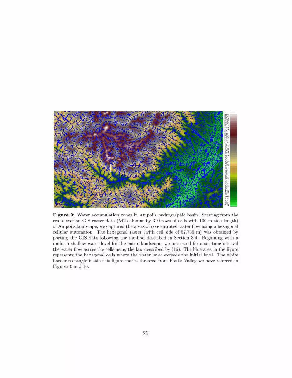
Figure 9: Water accumulation zones in Ampoi’s hydrographic basin. Starting from thereal elevation GIS raster data (542 columns by 310 rows of cells with 100 m side length)of Ampoi’s landscape, we captured the areas of concentrated water flow using a hexagonalcellular automaton. The hexagonal raster (with cell side of 57.735 m) was obtained byporting the GIS data following the method described in Section 3.4. Beginning with auniform shallow water level for the entire landscape, we processed for a set time intervalthe water flow across the cells using the law described by (16). The blue area in the figurerepresents the hexagonal cells where the water layer exceeds the initial level. The whiteborder rectangle inside this figure marks the area from Paul’s Valley we have referred inFigures 6 and 10.

26

the water accumulation zones found in two different ways. It is known that ifTarboton’s rules are used, then there is the possibility that the flow directionin some cells cannot be defined. To overcome this problem, Tarboton usesspecial treatments for such cells. The iterative process (based on Tarboton)implemented by us only uses the basic rules without any improvement andthis can be a reason of why the water accumulation zones from the picturein the middle are so spread out.

Figure 10: Potential water accumulation zones in Paul’s Valley. The left figure is aphoto of this region taken from the airplane. The relief from the image in the middleis given by the same 130 × 240 GIS raster data with square cells of 10 m size used forthe middle picture from Figure 6. The relief from the right picture is generated from thehexagonal raster (of 5.7735 m cell size) obtained by applying ENO DP to the same GISraster used for the middle image. The blue transparent areas represent the potential wateraccumulation zones determined by an iterative process of type (17). The picture in themiddle is obtained using Tarboton’s rules for water change among cells. For the pictureon the right side, we used our water routing method described in this section. One clearlyobserves that the accumulation zones indicated by this method overlap almost perfectlythe ravines and are less spread than the ones identified in the middle image.

5 Conclusions and Remarks

We provided a method for porting rectangular raster data on to hexagonalraster. The basic idea of the algorithm is to use an intermediate function

27

g that interpolates the rectangular raster function gr and then define thehexagonal raster function gh as the point values of g at the center of thehexagonal cell. The interpolation method can be extended to a less regulargrid and can be also used (see A) to recover missing data or to filter outliers.Using some theoretical as well as some practical examples, we show that theextension function is closer to the function represented by raster data thanraster function itself. As comparing to a well known cubic spline interpolant(CRS), Catmull-Rom (see Figure 5), ENO and CRS method have the samedegree of accuracy, but CRS is faster than ENO method, and furnishes asmooth function in contrast with almost continuous function obtained byENO method (see also Remark 1 in A for more theoretical details). Themain argument for using ENO instead of CRS is that ENO method doesnot introduce spurious oscillations for cases of data with large gradients andworks on a less regular grid points. For the case of digital terrain model,it is crucial to preserve the terrain shape and not to introduce artifacts.Both methods also provide a good compromise between a reduced amountof computational effort and the accuracy of the extended function.

The OF is an unsupervised outlier detection method and tries to recognizean abnormal point in a well defined neighborhood by evaluating the variationof the bicubic interpolant polynomials; an outlier is then detected since itintroduces a larger variation than the neighboring regular points do. Themethod assumes some “smoothness” on these regular points and a certainsparsity of the outlier distributions. We point out that OF eliminates adetected outlier from the set of data used in the interpolation algorithm.The theoretical example presented in Section 4.1 and other data simulationsnot included in this paper encourage us to step further into this direction.

Table 4 compares features of our methods (ENO, OF), CRS, and Id (theextension function of Id is identical to the raster function). The numbers fromthe accuracy column represent the maximal degree of polynomials which canbe exactly reconstructed. The property of recovering polynomials is closelyrelated to the approximation order of the method. Data Recovery means thecapability of the method to supply the missing data from a raster; an exampleof numerical errors in this matter is presented in Table 2. Row like grids canbe pictured as points being arranged along parallel lines; for a mathematicaldefinition, see A. The fidelity feature refers to the capacity of the methodto preserve the qualitative shape of the function one has to reconstruct (thefidelity of a method should not be confused with the accuracy, see Figure 5for two pictures of same accuracy but different shapes); the Id extension

28

function keeps the shape of the point distribution. A ranking of the methodsfrom the speed point of view is given in the last column, 1 for the fastest.

Table 4: The main features of the interpolation methods discussed in this paper.

Method Accuracy DataRecovery

Grid Fidelity OutlierDetection

Speed(rank)

ENO 3 Yes row like high No 3OF 3 Yes row like unknown Yes 3CRS 3 No regular medium No 2Id 0 No any neutral No 1

The water routing method presented in the Section 4.2 has a physicalbase and it is a simplified version of a discrete form of shallow water equa-tions. One of the advantage of this approach is the use of hexagonal rasterthat benefits from the higher isotropy of hexagonal cells which allow a moresuitable modelling of the transport phenomena. Another advantage of thisapproach is that it can be incorporated in more elaborated water flow modelsas a first step for a very quick investigation of the terrain topography andthe potential water accumulation.

Further research directions include:

1. To develop the software in order to be compatible with variables havingrestrictions on the size and form of the discretization unit as a resultof the observation scale and method.

(a) to add other tessellations and irregular partitions, exposed as con-figurable user inputs;

(b) to compute the value for each polygon in the plane partition in twovariants: at its center and by the average value of the intermediatefunction in the polygon, exposed as configurable user inputs;

(c) to develop an algorithm for nominal DP.

2. To construct a user friendly interface for the DP tool.

3. To develop a multiresolution analysis by using cubic spline wavelets inorder to examine the GIS data (data de-noising and compression willbe also considered).

29

Remarks Concerning the Asterix Porting Data Software- The downloadable version of the Asterix Porting Data Software availableon the web is part of a larger package in development. The current versioncontains the ENO scheme, the construction of a hexagonal raster, and theDP from a GIS to a hexagonal raster. In addition, a tool for plotting thehexagonal raster is also included.- This version does not contain examples of all the theoretical and numericalresults from the article. Readers who are interested in these examples areasked to email the authors.- The software is available under GPL license and contains the necessarydocumentation for its usage.

Acknowledgment

This work was performed within the project 50/2012 ASPABIR(www.aspabir.biogeochemistry.ro) funded by Executive Agency for HigherEducation, Research, Development and Innovation Funding, Romania (UE-FISCDI). The authors acknowledge Florian Bodescu, who provided the digi-tal terrain model. They specially thank all four anonymous reviewers for theconstructive criticism that greatly improved the manuscript.

A Essentially Non-Oscillating Extension Al-

gorithm

Here we present some details about the ENO algorithm and we extend it toa less regular net of points. Let D be a rectangular domain

D := (x, y) ∈ R2 | a ≤ x ≤ b, c ≤ y ≤ d,

where a, b, c, d are some arbitrarily fixed real numbers. We call a row likegrid in D any set N of the form

N := Pi,j = (xji , yj) ∈ D | i = 1, Nj, j = 1,M, (18)

where a <= xj1 < . . . < xjNj <= b for all j = 1,M and c <= y1 < . . . <yM <= d. Note that the net has a variable number of knots on the linesy = yj and distance between two consecutive yk and yk+1 is also variable.

Let L∞(D) be the space of bounded functions on D and R := g :N → R the space of reticulated functions. One defines the restriction

30

operator R : L∞(D)→ R by R(G)(Pi,j) = G(Pi,j) for all Pi,j ∈ N . We callL : R → L∞(D) the extension operator.

To find the extension polynomial at an interval Iξk , one needs to solve theminimization problem (6) which involves the calculation of the quantity

d kp,q :=∥∥∥Pf ;(p,q)

(k,k+1) −Qfk

∥∥∥2

L2(Iξk). (19)

By standard calculation, we have

d kp,q = c ·(

(λkp,q)2 + (µkp,q)

2 + 3/2 · λkp,qµkp,q), (20)

whereδkp,q = (ξk+1 − ξk)[ξk; ξk+1; ξp; ξq]f,

λkp,q :=ξk − ξpξk+1 − ξk

δkp,q + [ξk; ξk+1; ξp]f,

µkp,q := λkp,q + δkp,q.

(21)

and c is a constant independent of the knots p and q. Using (20) and (21),the minimization step in the algorithm (6) can be reformulated as:

Find i, j s.t. (ξi, ξj) = arg minξp,ξq

d kp,q,

with the pair (p, q) ∈ (k − 2, k − 1), (k − 1, k + 2), (k + 2, k + 3).(22)

Let lξ stand for the 1D continuous extension operator from the space ofreticulated functions to the space of continuous functions. The algorithm toevaluate the 1D extension operator lξ read as:

31

Algorithm 1. The 1D ENO Algorithm

Data Input: ξii=1,N , f : ξii=1,N → R; ξ.Data Output: lξ(f)(ξ).

1. Find Iξk such that ξ ∈ Iξk .

2. Define Sξk of the form (5).

3. Find the knots ξi, ξj using (22).

4. Set lξ(f)(ξ) := Pf ;(i,j)(k,k+1)(ξ).

Note that the extension 1D ENO algorithm can also be applied for thepoints ξ outside the interval [ξ1, ξN ], using the following formula

lξ(f)(ξ) =

Pf ;(3,4)

(1,2) (ξ), for ξ < ξ1

Pf ;(N−3,N−2)(N−1,N) (ξ), for ξ > ξN

. (23)

Now, having the 1D ENO scheme (22) and (23), one can set up the algorithmto define the 2D extension operator L.

Algorithm 2. The 2D ENO Algorithm

Data Input: D,N , g : N → R; (x, y) ∈ DData Output: L(g)(x, y).

1. Find Iyk such that y ∈ Iyk .

2. Define Syk of the form (5).

3. For each m s.t. ym ∈ Syk , using Algorithm 1, calculatefm(x) := lx(g(·, ym))(x)

4. Set L(g)(x, y) := ly(f(x, ·))∣∣∣Iyk

(y).

In this algorithm, lx and ly denotes the 1D extension operators withrespect to Ox and Oy knots, respectively. The notation lx(g(·, ym)) from

32

Step 3 reads as follows: the extension operator lx acts on the reticulatedfunction g(·, ym) having the values g(xmi , ym) on the Ox knots xmi i=1,Nm .Also, f(x, ·) from Step 4 represents the reticulated function having the valuesf(x, ym) = fm(x) on the Oy knots ym ∈ Syk .

Remark 1 Essentially, the 2D ENO extension operator L is given by

L(g) := (ly lx)(g).

For the 2D ENO extension function the following properties hold:

1. L(g)(Pij) = g(Pij), for all g ∈ R.

2. L(G)=G, for all G ∈ π3,3

3. L(g) is always continuous with respect to y and continuous with respectto x except for a finite number of points.

4. If when on Step 4 of Algorithm 2 the problem (22) does not have aunique solution for a particular x, then (x, y) is possibly a discontinuitypoint of the extension function g. Otherwise, g is locally continuous at(x, y).

Remark 2 Algorithm 1 and Algorithm 2 can be easily adapted for the OFinterpolation method.

B Details on test rasters from Section 4.1.2

The test rasters we used in Section 4.1.2 are constructed as it follows.Let δ be the cell size of the square basis raster, and m, n some positive

integers. In order to construct a square test raster, we randomly eliminaterows of cells except the top and bottom rows, such that the distance betweenany two consecutive remaining rows does not exceed mδ. Then, for eachof the remaining rows, we randomly eliminate cells except the first and lastones, such that the distance between any two consecutive remaining cellsdoes not exceed nδ. The Figure 11 gives the correspondence between thetest index α and the parameters m, n, and an example of a possible pointdistribution of the kept data in the grid for such test.

33

α m n1 3 32 4 33 5 34 5 45 5 5

0

20

40

60

80

100

120

140

160

0 50 100 150 200 250 300

Figure 11: The correspondence between the test raster index α and the parameters m,n, and a snapshot example (the lower left corner) of a point distribution in the grid forα = 5 and δ = 10 m.

References

[1] J. M. Baetens, D.K. Loof, and D. B. Baets. Influence of the topology ofa cellular automaton on its dynamical properties. Commun. NonlinearSci. Numer. Simulat., 18:651–668, 2013.

[2] Colin P.D. Birch, Sander P. Oom, and Jonathan A. Beecham. Rectangu-lar and hexagonal grids used for observation, experiment and simulationin ecology. Ecological Modelling, 206:347–359, 2007.

[3] John M. Chambers. Software for Data Analysis: Programming with R.Springer, 2008.

[4] N. Chiba, K. Muraoka, and K. Fujita. An erosion model based onvelocity fields for the visual simulation of mountain scenery. Journal ofVisualization and Computer Animation, 9:185–194, 1998.

[5] Noel A. C. Cressie. Statistics for Spatial Data. Wiley, revised editionedition, January 1993.

[6] D. D’Ambrosio, S. Di Gregorio, S. Gabriele, and R. Gaudio. A cellularautomata model for soil erosion by water. Physics and Chemistry of theEarth, Part B: Hydrology, Oceans and Atmosphere, 26(1):33–39, 2001.

34

[7] D. D’Ambrosio, S. Di Gregorio, S. Gabriele, and R. Gaudio. Il modelload automi cellulari scavatu per la simulazione dell’erosione del suoloe del trasporto solido nei bacini idrografici: specificazione della parteidrodinamica nel caso di reticolo a celle esagonali regolari. TechnicalReport 586, Consiglio Nazionale delle Ricerche Istituto di Ricerca perla Protezione Idrogeologica, giugno 2002.

[8] Luıs de Sousa, Nery Fernanda, Sousa Ricardo, and Matos Joao. As-sessing the accuracy of hexagonal versus square tiled grids in preservingDEM surface flow directions. In Proceedings of the 7th InternationalSymposium on Spatial Accuracy Assessment in Natural Resources andEnvironmental Sciences (Accuracy 2006), pages 191–200. Instituto Ge-ographico Portugues, 2006.

[9] Neil Antony Dodgson. Image resampling. Technical Report UCAM-CL-TR-261, University of Cambridge, Computer Laboratory, August 1992.

[10] Olivier Dubrule. Two methods with different objectives: Splines andkriging. Journal of the International Association for Mathematical Ge-ology, 15(2):245–257, 1983.

[11] Shelly Eberly, Jenise Swall, David Holland, Bill Cox, and EllenBaldridge. Developing spatially interpolated surfaces and estimatinguncertainty. Technical Report EPA-454/R-04-004, Office of Air QualityPlanning and Standards, Office of Air and Radiation, U.S. Environmen-tal Protection Agency, November 2004.

[12] David Favis-Mortlock, Tony Guerra, and John Boardman. Aself-organizing dynamic systems approach to hillslope rill initiationand growth: model development and validation. In W. Summer,E. Klaghofer, and W. Zhang, editors, Modelling Soil Erosion, Sedi-ment Transport and Closely Related Hydrological Processes, pages 53–62.IAHS Publication no. 249, July 1998.

[13] Mark A. Fonstad. Cellular automata as analysis and synthesis enginesat the geomorphology ecology interface. Geomorphology, 77:217–234,2006.

[14] U. Frisch, B. Hasslacher, and Y. Pomeau. Lattice-gas automata for thenavier-stokes equation. Phys. Rev. Lett., 56:1505–1508, Apr 1986.

35

[15] Thierry Gallouet, Jean-Marc Herard, and Nicolas Seguin. Some ap-proximate godunov schemes to compute shallow-water equations withtopography. Computers & Fluids, 32(4):479–513, 2003.

[16] Antony Galton. Fields and objects in space, time, and space-time. Spa-tial Cognition and Computation, 1:39–68, 2004.

[17] R. H. Gardner, T. R. Lookingbill, P. A. Townsend, and J. Ferrari. A newapproach for rescaling land cover data. Landscape Ecology, 23:53–526,2008.

[18] M. F. Goodchild. Geographical data modeling. Computers and Geo-sciences, 8:401–408, 1992.

[19] M. C. Gough and S. P. Rushton. The application of gis-modelling tomustelid landscape ecology. Mammal Rev., 30:197–216, 2000.

[20] Julian Hagenauer and Marco Helbich. Contextual neural gas for spatialclustering and analysis. International Journal of Geographical Informa-tion Science, 27(2):251–266, 2013.

[21] Ami Harten, Bjorn Engquist, Stanley Osher, and Sukumar RChakravarthy. Uniformly high order accurate essentially non-oscillatoryschemes, iii. Journal of Computational Physics, 71(2):231–303, August1987.

[22] Ami Harten, Stanley Osher, Bjrn Engquist, and Sukumar R.Chakravarthy. Some results on uniformly high-order accurate essentiallynonoscillatory schemes. Applied Numerical Mathematics, 2:347–377, Oc-tober 1986.

[23] Amy Hillier. Manual for working with arcgis 10, 2011.

[24] E. E. Holmes, M. A. Lewis, J. Banks, and R. R. Veit. Partial differen-tial equations in ecology: spatial interactions and population dynamics.Ecology, 75:17–29, 1994.

[25] M. F. Hutchinson. A new procedure for gridding elevation and streamline data with automatic removal of spurious pits. Journal of Hydrology,106:211–232, 1989.

36

[26] Stelian Ion and Dorin Marinescu. Spline wavelets analysis of reticu-lated functions on bounded interval. Mathematical Reports, 4(2):191–205, 2002.

[27] V. Iordache, S. Ion, and A. Pohoata. Integrated modeling of metalsbiogeochemistry: potential and limits. Chem Erde Geochem, 69:125–169, 2009.

[28] V. Iordache, E. Kothe, A. Neagoe, and F. Gherghel. A conceptualframework for up-scaling ecological processes and application to ecto-mycorrhizal fungi. In M. Rai and A. Varma, editors, Diversity andbiotechnology of ectomycorrhizae, pages 255–299. Springer, 2011.

[29] V. Iordache, R. Lacatusu, D. Scradeanu, M. Onete, D. Jianu, F. Bode-scu, A. Neagoe, D. Purice, and I. Cobzaru. Contributions to the theo-retical foundations of integrated modeling in biogeochemistry and theirapplication in contaminated areas. In E. Kothe and A. Varma, edi-tors, Bio-geo interactions in metal-contaminated soils, volume 31, pages385–416. Springer, 2012.

[30] Bin Jiang. Extraction of spatial objects from laser-scanning data usinga clustering technique. In XXth ISPRS Congress: Geo-Imagery bridgingcontinents, volume 3, pages 219–224, 2004.

[31] J. Kumhalova, F. Kumhala, P. Novak, and S Matejkova. Airborne laserscanning data as a source of field topographical characteristics. Plant,Soil and Environment, 59(9):423–431, 2013.

[32] Seungyong Lee, George Wolberg, and Sung Yong Shin. Scattered datainterpolation with multilevel b-splines. IEEE Transactions on Visual-ization and Computer Graphics, 3(3):228–244, July-September 1997.

[33] Thomas M. Lehmann, Claudia Gonner, and Klaus Spitzer. Survey:interpolation methods in medical image processing. IEEE Transactionson Medical Imaging, 18:1049–1075, November 1999.

[34] David J. C. MacKay. Bayesian interpolation. Neural Computation,4:415–447, 1992.

37

[35] G. Matheron. Splines and Kriging; their formal equivalence. In D. F.Merriam, editor, Down-to-Earth Statistics: Solutions looking for Geolog-ical Problems, pages 77–95. Syracuse University Geology Contributions,1981.

[36] L. Mitas and H. Mitasova. Spatial interpolation. In P. Longley, M. F.Goodchild, D. J. Maguire, and D. W. Rhind, editors, Geographical Infor-mation Systems: Principles, Techniques, Management and Applications,volume 1, pages 481–492. Wiley, 1999.

[37] Don P. Mitchell and Arun N. Netravali. Reconstruction filters incomputer-graphics. SIGGRAPH Comput. Graph., 22(4):221–228, June1988.

[38] Jane Molofsky and James D. Bever. A new kind of ecology? BioScience,54(5):440–446, 2004.

[39] I. D. Moore, R. B. Grayson, and A. R. Ladson. Digital terrain modelling:a review of hydrological, geomorphological, and biological applications.Hydrological Processes, 5:3–30, 1991.

[40] Eder Paulo Moreira, W.J. Elliot, and A.T. Hudak. Effects of dtm res-olution on slope steepness and soil loss prediction on hillslope profiles.In The XXXIII Brazilian Congress of Soil Science symposium, Soils:Climate change and sustainability, 2011.

[41] John F. O’Callaghan and David M. Mark. The extraction of drainagenetworks from digital elevation data. Computer Vision, Graphics, andImage Processing, 28(3):323–344, 1984.

[42] Jon D. Pelletier. Minimizing the grid-resolution dependence of flow-routing algorithms for geomorphic applications. Geomorphology, 122(1-2):91–98, 2010.

[43] P. Quinn, K. Beaven, P. Chevallier, and O. Planchon. The prediction ofhillslope flow paths for distributed hydrological modelling using digitalterrain models. Hydrological Processes, 5(1):59–79, 1991.

[44] K. Sahr. Hexagonal discrtete global grid systems for geospatial com-puting. Archives of Photogrammetry, Cartography and Remote Sensing,22:363–376, 2011.

38

[45] I.J. Schoenberg. Cardinal Spline Interpolation, volume CBMS-NSF Re-gional Conference Series in Applied Mathematics 12. Capital City Press,Montpelier, Vermont, second printing edition, 1993.

[46] Jan Seibert and Brian L. McGlynn. A new triangular multiple flowdirection algorithm for computing upslope areas from gridded digitalelevation models. Water Resources Research, 43(4), 2007.

[47] Elisabete A. Silva, Jack Ahern, and Jack Wileden. Strategies for land-scape ecology: An application using cellular automata models. Progressin Planning, 70:133–177, November 2008.

[48] S. L. Smith, D. A. Holland, and P. A. Longley. The importance of under-standing error in lidar digital elevation models. International Archives ofthe Photogrammetry, Remote Sensing and Spatial Information Sciences,35:996–1001, 2004.

[49] Pierre Soille, Jrgen Voght, and Roberto Colombo. Carving and adaptivedrainage enforcement of grid digital elevation models. Water ResourcesResearch, 39(12):1366–1375, 2003.

[50] Shruthi Srinivasan, Sorin C. Popescu, Marian Eriksson, Ryan D. Sheri-dan, and Nian-Wei Ku. Multi-temporal terrestrial laser scanningfor modeling tree biomass change. Forest Ecology and Management,318(0):304–317, 2014.

[51] Christoph Stasch, Simon Scheider, Edzer Pebesma, and Werner Kuhn.Meaningful spatial prediction and aggregation. Environmental Mod-elling&Software, 51:149–165, 2014.

[52] David G. Tarboton. A new method for the determination of flow direc-tions and upslope areas in grid digital elevation models. Water ResourcesResearch, 33(2):309–319, 1997.

[53] C. Varekamp, A. K. Skidmore, and P. A. B. Burrough. Using public do-main geostatistical and gis software for spatial interpolation. Photogram-metric Engineering and Remote Sensing, 62(7):845–854, July 1996.

[54] R. F. Vazquez and J. Feyen. Assessment of the effects of dem gridding onthe predictions of basin runoff using mike she and a modelling resolutionof 600 m. Journal of Hydrology, 334:73–87, 2007.

39

[55] Alexey Voinov and Herman H. Shugart. ’integronsters’, integral andintegrated modeling. Environmental Modeling&Software, 39:149–158,2013.

[56] J. P. Walker and G. R. Willgoose. On the effect of digital elevation modelaccuracy on hydrology and geomorphology. Water Resources Research,35(7):2259–2268, 1999.

[57] Yu Wei, Xuemei Li, Jie Wang, Caiming Zhang, and Yi Liu. Graphcuts image segmentation in a hexagonal-image processing framework.Journal of Computational Information Systems, 8(14):5953–5960, 2012.

[58] Marco J. Van De Wiel, Tom J. Coulthard, Mark G. Macklin, and JohnLewin. Embedding reach-scale fluvial dynamics within the caesar cellu-lar automaton landscape evolution model. Geomorphology, 90:283–301,2007.

[59] John P. Wilson, Christine S. Lam, and Yongxin Deng. Comparison ofthe performance of flow-routing algorithms used in gis-based hydrologicanalysis. Hydrological Processes, 21(8):1026–1044, 2007.

[60] Dieter Wolf-Gladrow. Lattice-gas cellular automata and lattice Boltz-mann models an introduction. Springer, 1st edition, March 2000.

40