evaluating the performance of cost-based discretization versus entropy- and error-based...

Computers & Operations Research 33 (2006) 3107–3123www.elsevier.com/locate/cor

Evaluating the performance of cost-based discretization versusentropy- and error-based discretization

Davy Janssens, Tom Brijs, Koen Vanhoof, Geert Wets∗

Limburgs Universitair Centrum, Research Group Data Analysis and Modelling, Universitaire Campus, Gebouw D,B-3590 Diepenbeek, Belgium

Available online 12 February 2005

Abstract

Discretization is defined as the process that divides continuous numeric values into intervals of discrete categoricalvalues. In this article, the concept of cost-based discretization as a pre-processing step to the induction of a classifier isintroduced in order to obtain an optimal multi-interval splitting for each numeric attribute. A transparent descriptionof the method and the steps involved in cost-based discretization are given. The aim of this paper is to present thismethod and to assess the potential benefits of such an approach. Furthermore, its performance against two otherwell-known methods, i.e. entropy- and pure error-based discretization is examined. To this end, experiments on 14data sets, taken from the UCI Repository on Machine Learning were carried out. In order to compare the differentmethods, the area under the Receiver Operating Characteristic (ROC) graph was used and tested on its level ofsignificance. For most data sets the results show that cost-based discretization achieves satisfactory results whencompared to entropy- and error-based discretization.

Given its importance, many researchers have already contributed to the issue of discretization in the past. However,to the best of our knowledge, no efforts have been made yet to include the concept of misclassification costs to findan optimal multi-split for discretization purposes, prior to induction of the decision tree. For this reason, this newconcept is introduced and explored in this article by means of operations research techniques.� 2005 Elsevier Ltd. All rights reserved.

Keywords: Discretization; ROC-curve; Cost-sensitive learning

∗ Corresponding author. Tel.: +32 011 26 86 49; fax: +32 011 26 87 00.E-mail addresses: [email protected] (D. Janssens), [email protected] (T. Brijs), [email protected]

(K. Vanhoof), [email protected] (G. Wets).

0305-0548/$ - see front matter � 2005 Elsevier Ltd. All rights reserved.doi:10.1016/j.cor.2005.01.022

http://www.elsevier.com/locate/cor

mailto:[email protected]




3108 D. Janssens et al. / Computers & Operations Research 33 (2006) 3107–3123

1. Introduction

Highly non-uniform misclassification costs are very common in a variety of challenging real-world datamining problems, such as fraud detection, medical diagnosis and various problems in business decision-making. In many cases, the distribution among the classes is skewed but the cost of not recognizing someof the examples belonging to the minority class is high. In medicine for instance, the cost of prescribinga drug to an allergic patient can be much higher than the cost of not prescribing the drug to a non-allergic patient, if alternative treatments are available. Various cost-sensitive classification systems havebeen developed that are able to deal adequately with this problem. The idea has also gained increasingattention during recent years [1].

However, to the best of our knowledge, the idea to take misclassification costs into account whendiscretizing continuous numeric attributes prior to induction has not been proposed yet. Discretization isdefined as the process that divides continuous numeric values into intervals of discrete categorical values[2]. Given its importance, many researchers have already contributed to this research domain in the past[3–8] in the context of machine learning classification systems. Some classification systems such as C4.5[9] and CART [10] for instance, originally were not designed to handle continuous numeric attributes verywell. Therefore, during the construction of these classifiers, continuous attributes are now divided intodiscrete categorical values by grouping continuous values together. Discretization techniques are not onlyfrequently adopted in decision tree classifiers, but also in the context of many other learning paradigms,such as Bayesian inference [11,12], instance-based learning [13], inductive logic programming [14] andgenetic algorithms [15]. Sometimes continuous values are discretized on-the-fly (i.e. during the construc-tion of the learning paradigm), but often discretization can also be carried out as a pre-processing stepbefore the induction of the classifier. In this case, discretization itself may be considered as a form ofknowledge discovery in that critical values in a continuous domain may be revealed [16]. Taking misclas-sification costs into account seems justified to identify these critical values when dealing with non-uniformmisclassification costs, as for instance in the example above. Also, according to Catlett [17], for very largedata sets, discretization as a pre-processing step significantly reduces the time to induce a classifier.

For the reasons mentioned above, the objective of this paper is to introduce the concept of cost-baseddiscretization to assess the potential benefits. In order to test this, its performance is evaluated against twoother well-known discretization methods, i.e. entropy- and error-based discretization. An evaluation isonly made in the context of decision tree learning, but the performance of the technique can be evaluatedfor other classification systems as well.

This paper is organized as follows. In Section 2 a brief overview of the existing literature on discretiza-tion is provided. From a conceptual point of view, the effectiveness of cost-based discretization in findingthe critical cutpoints that minimize an overall cost function is explained in Section 3 and the methodologybehind cost-based discretization is shown by means of an example. In Section 4 an empirical evaluationof these methods is carried out on several data sets, taken from the UCI Repository on Machine Learning[18]. Finally, some conclusions and recommendations for further research are presented in Section 5.

2. Discretization methods

In essence, the process of discretization involves the grouping of continuous values into a number ofdiscrete intervals. However, the decision which continuous values to group together, how many intervals

D. Janssens et al. / Computers & Operations Research 33 (2006) 3107–3123 3109

to generate, and thus where to position the interval cutpoints on the continuous scale of attribute valuesis not always identical for the different discretization methods. Therefore, a brief literature overview ofprevious research on discretization is presented. This overview can be characterized along five differentaxes [12]: the type of evaluation function being used, global versus local, static versus dynamic, supervisedversus unsupervised and top-down versus bottom-up discretization.

2.1. Evaluation function

Since discretization involves grouping continuous values into discrete intervals, all discretization meth-ods differ with respect to how they measure the quality of the partitioning. Error-based methods, suchas for example Maass [19], evaluate candidate cutpoints against an error function and explore a searchspace of boundary points to minimize the sum of false positive (FP) and false negative (FN) errors on thetraining set. In other words, given a fixed number of intervals, error-based discretization aims at findingthe best discretization that minimizes the total number of errors (FP and FN) made by grouping togetherparticular continuous values into an interval. An alternative efficient approach can be found in [20]. How-ever, as mentioned above, the concept of introducing costs into the discretization process has not yetbeen proposed or evaluated before. Also, indirect ways for doing this, for instance by incorporating in-stance weighting and subsequently applying error-based discretization was not yet tested. Entropy-basedmethods, such as for example Fayyad and Irani [3], are among the most commonly used discretizationmeasures in the literature. These methods use entropy measures to evaluate candidate cutpoints. Thismeans that an entropy-based method will use the class information entropy of candidate partitions toselect boundaries for discretization. Class information entropy is a measure of purity and it measures theamount of information which would be needed to specify to which class an instance belongs. It considersone big interval containing all known values of a feature and then recursively partitions this interval intosmaller subintervals until some stopping criterion, for example Minimum Description Length Principle(MDLP) [21] or an optimal number of intervals is achieved. Other evaluation measures include Gini,dissimilarity and the Hellinger measure.

2.2. Global versus local discretization

The distinction between global [22] and local [9] discretization methods is dependent on whendiscretization is performed. Global discretization handles discretization of each numeric attribute asa pre-processing step, i.e. before induction of a classifier whereas local methods, like C4.5 carry outdiscretization on-the-fly (during induction). Empirical results have indicated that global discretizationmethods often produced superior results compared to local methods since the former use the entire valuedomain of a numeric attribute for discretization, whereas local methods produce intervals that are appliedto subpartitions of the instance space [12].

2.3. Static versus dynamic discretization

The distinction between static [17,3,4,23] and dynamic [5,6] methods depends on whether the methodtakes feature interactions into account. Static methods, such as binning, entropy-based partitioning andthe 1R algorithm, determine the number of partitions for each attribute independent of the other features.


In contrast, dynamic methods conduct a search through the space of possible k partitions for all featuressimultaneously, thereby capturing interdependencies in feature discretization.

2.4. Supervised versus unsupervised discretization

Another distinction can be made dependent on whether the method takes class information into accountto find proper intervals or not. Several discretization methods, such as equal width interval binning orequal frequency binning, do not make use of class membership information during the discretizationprocess. These methods are referred to as unsupervised methods [24]. In contrast, discretization methodsthat use class labels for carrying out discretization are referred to as supervised methods [23,3]. Previousresearch has indicated that supervised methods are better than unsupervised methods [12].

2.5. Top-down versus bottom-up discretization

Finally, the distinction between top-down [3] and bottom-up [25] discretization methods can be made.Top-down methods consider one big interval containing all known values of a feature and then partitionthis interval into smaller and smaller subintervals until a certain stopping criterion, for example MinimumDescription Length (MDLP), or optimal number of intervals is achieved. In contrast, bottom-up methodsinitially consider a number of intervals, determined by the set of boundary points, to combine theseintervals during execution until a certain stopping criterion, such as a �2 threshold, or optimal number ofintervals is achieved.

The cost-based discretization method presented in this paper, is an error-based, global, static, supervisedmethod combining a top-down and bottom-up approach. However, it is not just an error-based method. Bymeans of the introduction of a misclassification cost matrix, boundary points are evaluated against a costfunction (instead of an error function) to minimize the overall misclassification cost of errors instead ofjust the total sum of errors. It is a global method, since discretization is carried out as a pre-processing stepto induction. Furthermore, cost-based discretization is static, since we discretize each attribute separately.It is supervised, since we use class information to find an optimal interval partitioning. Finally, it combinesa top-down with a bottom-up approach since all the boundary points are evaluated simultaneously by aninteger programming approach.

3. Cost-based discretization

The objective of our cost-based discretization approach is to take into account the cost of making errorsinstead of just minimizing the total sum of errors, such as in error-based discretization. The specificationof this cost function is dependent on the costs assigned to the different error types. In the special casewhere the cost of making errors is equal, the introduced method of cost-based discretization is in factequal to error-based discretization. In this case, the concept of the method presented in this paper is alsocomparable to the work described by Maass [19] and Elomaa and Rousu [20].

In order to understand our contribution of cost-based discretization, it is shown in the next section thatthe intervals produced by error-based discretization cannot be optimal in a situation where the costs ofFP and FN errors are unequal.


aC1 C2 C3 C4 C5 A

k

lY

Frequency

X

Fig. 1. Cutpoints and class distribution for a continuous attribute A.

3.1. Finding optimal cutpoints for cost-based discretization

Suppose we have an attribute A and a binary target variable with class values ‘X’ and ‘Y’. ‘X’ and ‘Y’have equally sized frequency distributions but the second distribution is shifted in a way that they havea non-empty intersection (see Fig. 1). Finding the optimal discretization in this case would then involvethe identification of all boundary points.

Formally, the concept of a boundary point is defined as: “A value T in the range of the attribute A isa boundary point if in the sequence of examples sorted by the value of A, there exist two examples s1,s2 ∈ S, having different classes, such that valA(s1) < T < valA(s2); and there exists no other examples′ ∈ S such that valA(s1) < valA(s′) < valA(s2)” [26].

In this original definition, there are infinitely many real numbers in between two values that would allqualify as boundary points. In order to fix one particular value and to make the selected value unique, theaverage of the two points valA(s1) and valA(s2) is taken. Second, and according to the work described in[27], the definition above does not group together attribute values with an equal relative class frequencydistribution. In [27], this idea is explored and the resulting points are called “segment borders” insteadof boundary points. Segment borders are thus a subset of boundary points. This means that less potentialcutpoints need to be examined in order to recover the optimal split of the data. Also, the additionalcost for using segment borders in splitting is marginal, as the cost is maximized by the O(n log n) timerequirement of sorting, which cannot be avoided. For this reason, adjacent splits with an equal relative classdistribution are grouped together for computational efficiency reasons in the experiments of this study.

To summarize, a boundary point is a value V that is strictly in the middle of two sorted attribute valuesU and W such that all examples having attribute value U have a different class label compared to theexamples having attribute value W or U and W have a different class frequency distribution.

Among all identified boundary points (which are not all shown in Fig. 1 for clarity), C1 . . . C5 areimportant candidate cutpoints for error-based discretization. In this example, when attribute A has avalue in the interval [C1, C2] or [C2, C3] ‘X’ is the predicted class label, otherwise ‘Y’. Therefore, theerror-based discretization method, aiming at minimizing the total sum of errors, will merge [C1, C2] and[C2, C3] into [C1, C3] with label ‘X’, and [C3, C4] and [C4, C5] into [C3, C5] with label ‘Y’, respectively.However, in the cost-based discretizer, the goal is to minimize the total cost of misclassifications insteadof the total sum of errors. In order to calculate this cost, a misclassification cost is assigned to every errortype (FP and FN). For instance, assume that misclassifying ‘X’ is twice as costly as misclassifying ‘Y’.In that case, given the candidate cutpoints for error-based discretization, the cost-based discretizer will


Table 1Example of cost-based discretization

Attribute value Class value Attribute value Class value Attribute value Class value

49 Y 51 Y 60 Y37 Z 3 X 32 Y41 Y 7 X 34 Y11 X 43 Y 30 X24 Z 56 Y 45 Y

merge [C1, C2], [C2, C3] and [C3, C4] into [C1, C4] due to the fact that the total number of X cases in[C3, C4] multiplied by 2 is larger than the number of Y cases in the same interval. The remaining twointervals [C1, C4] and [C4, C5] will minimize the total misclassification cost, given the positions of thecutpoints.

However, it is clear that the optimal solution for cost-based discretization has not yet been reached.The optimal solution is given by [C1, a] and [a, C5] where ‘a’ is the intersection point where it holdsthat |ak| = |kl|. In other words, the cost-based discretization technique will select a different boundarypoint to serve as the cutpoint for the two intervals, namely that particular attribute value after which themisclassification cost of ‘X’ by predicting the remaining attribute values to belong to class ‘Y’ is less thanthe misclassification cost of ‘Y’.

As it is illustrated in the example above, misclassifying ‘X’ was twice as costly as misclassifying ‘Y’.In reality, these values are often entered in a cost matrix. The number of entries in the matrix is thusdependent on the number of classes of the target attribute. This means that cost-based discretization isequally suitable for multi-class discretization. For instance, it can be said that misclassifying ‘X’ is twiceas costly as misclassifying ‘Y’ but that misclassifying ‘X’ is even three times as costly as misclassifying‘Z’. Similarly, the total minimum cost of misclassifications can be calculated, since one particular class(that with the lowest cost) is assigned to a particular interval. For multi-class problems, the error typesare no longer limited to false negative and false positive errors.

3.2. Methodology

In order to illustrate the methodology behind cost-based discretization, in this section a hypotheticalexample of a continuous numeric attribute with 15 values and three class labels is considered. Thedistribution of the different attribute values together with their class values is given in Table 1.

In a first step, the method will sort the attribute values and will try to identify all boundary points. Forthe example cited above, seven boundary points were determined. The position of the different boundarypoints is illustrated in Fig. 2.

These boundary points will serve as potential cutpoints for our final discretization. In previous work[26] it has been proven that it is sufficient to consider boundary points as potential cutpoints when usingInformation Gain as the evaluation function, because optimal splits always fall on boundary points. Later,Elomaa and Rousu [28] extended this finding and showed the same to hold for other evaluation functionsas well. In the more recent work, the same authors (Elomaa and Rousu [29]) showed that evaluating aneven smaller set of points (subset of boundary points) suffices for many evaluation functions.


2 3 4 5 6 7

3 7 11 24 30 32 34 37 41 43 45 49 51 56 60

X X X Z X Y Y Z Y Y Y Y Y Y Y

1

Fig. 2. Sorted attribute values and distribution of class values with possible boundary points.

Table 2Intervals with the corresponding minimum costs

Interval Min. cost Interval Min. cost Interval Min. cost

1–2 0 2–4 1 3–7 21–3 3 2–5 2 4–5 01–4 3 2–6 3 4–6 11–5 5 2–7 3 4–7 11–6 6 3–4 0 5–6 01–7 6 3–5 1 5–7 12–3 0 3–6 2 6–7 0

As stated before, in order to calculate this cost a misclassification cost is assigned. For instance, assumethat misclassifying ‘X’ is twice as costly as misclassifying ‘Y’ and that misclassifying ‘X’ is even threetimes as costly as misclassifying ‘Z’. It is assumed that there is no difference in costs in misclassifying‘Y’ or in misclassifying ‘Z’. The minimal cost can then be calculated by multiplying the costs by theerrors made as a result of assigning one of the three classes to the interval and by picking the minimalcost of one of the three assignments. For instance, suppose we want to calculate the minimum cost in theinterval 1–5. Assigning the class value ‘X’ to the interval 1–5 results in three errors. The assumption wasmade that misclassifying ‘X’ is twice as costly as misclassifying ‘Y’ and that misclassifying ‘X’ coststhree times more than misclassifying ‘Z’ so the total cost will be: (2 ∗ 2) + (1 ∗ 3) = 7. Assigning theclass value ‘Y’ to the interval 1–5 results in five errors, so the total cost will be: (5 ∗ 1) = 5. Assigningthe class value ‘Z’ to the interval 1–5 results in six errors, so the total cost will be: (6 ∗ 1) = 6. Thismeans that for this interval the minimum cost is 5. The procedure for finding the minimum costs for theother intervals is similar and is shown in Table 2. Important to notice however is that for a real-worlddata set, it might be difficult to determine exact cost parameters. Therefore, cost values only reflect theirrelative importance against each other and also may depend on the user’s domain knowledge about theproblem.

The next step will be to set a maximum number of intervals (n) and to put the minimum costs of Table2 in a network, of which the size depends on the value of n. This value is a maximum value and as ourmethod chooses the total minimal cost of the network, the algorithm will still be able to choose lessintervals than the number specified by the user.

Suppose that in our example the value of n is set to 3, it is then possible to construct a network like theone shown in Fig. 3 (not all costs are included for the sake of clarity).


a11=0

a12=0

a13=3

a14=3 a15=5

a16=6

a17=6

1

2

3

4

5

6

7

c17=6

c27=3

c37=2

c47=1

c57=1

c67=0

c77=0

1

i

j

l

xij

yjk

zkl

2

3

4

5

6

7

1

7

k

Fig. 3. Shortest route network.

The optimization problem can then be formulated as follows:

MinimizeS =∑j

aij ∗ xij +∑

j,k�j

bjk ∗ yjk +∑

k

ckl ∗ zkl

Subject to∑j

xij = 1 and xij ; yjk; zkl ∈ {0, 1},∑k

zkl = 1, i ∈ {1},j ∈ {1, . . . , 7}

∀ j : ∑k�j

yjk = xij , k ∈ {1, . . . , 7},∀ k : ∑

j �k

yjk = zkl, l ∈ {7}.This is a typical formulation for the shortest path network, which is a well-known problem in operationsresearch [30]. The values xij , yjk and zkl are Boolean and represent whether the path is chosen or notchosen. The values aij , bjk and ckl represent the different costs to take a particular path. The position ofcutpoints can be determined by solving this shortest path problem by means of integer programming. Theactual size of the network for a particular data set and its corresponding optimization problem dependson the number of intervals (n) and the number of boundary points for the attribute to be discretized.

Therefore, generalizing the example given above to an arbitrarily number of intervals (n) and boundarypoints (B) gives us the following conceptualization of this problem:

Minimize S =B∑

d=1A11d

X11d+

n−1∑l=2

B∑o=1

B∑d �o

AlodXlod

+B∑

o=1AnoB

XnoB

s.t.B∑

d=1X11d

= 1 ∀l, ∀o, ∀d : Xlod∈ {0, 1}

B∑o=1

XnoB= 1, o, d ∈ {1, . . . , B}, ∀o :

B∑d �o

Xlod= Xl−1od

, l ∈ {2, . . . , n − 1},

∀ d :B∑

o�d

Xlod= Xl+1od

,


where B represents the number of Boundary points, n is the number of intervals in the network and o

and d are, respectively, the origin and destination nodes in each interval in the network. The variable A

represents the costs to take a particular path. Each variable A has an origin and destination node as itssubindex. The index � always appears as a subindex of the variable A and it represents the current intervalin the network. For instance the value A234 represents the cost of going from the third boundary point tothe fourth destination node and this in the second interval. The values X represent Boolean values whichdetermine whether the path is chosen or not in this formulation.

Since our network contains all minimum costs in each interval, the optimal solution of this minimizationproblem is guaranteed (i.e. the global minimum cost over all intervals is achieved). Alternatively, it mightalso be possible to reformulate this problem as a dynamic instead of an integer programming approach.This may increase efficiency and reduce computational complexity as it is for instance applied in [5,28,29]for non-cost-based discretization. However, we believe that representing cost-based discretization as ashortest path problem along with its optimal corresponding integer programming solution, benefits fromthe straightforward and clear implementation and from the conceptual simplicity to grasp the idea andthe importance of the cost-based discretization problem. Alternatively, existing error-based discretizationmethods could also be adapted by first applying instance weighting to generate an alternative cost-sensitivediscretization method. However, a cautionary note is needed in this case since it has been found in theprevious work [31] that instance weighting does not perform well (in terms of total misclassificationcosts) in data sets with highly skewed class distributions. Additional experiments are needed to evaluatewhether this deficiency is also present in the case when error-based discretization methods are adaptedthrough instance weighting.

Finally, it has to be said that, by increasing the error-cost of a particular class (e.g. class ‘X’ in theexample), the frequency of this class is leveraged so that this can result in different minimum costs and inanother positioning of the final cutpoints. Our method should therefore perform better than error-baseddiscretization because this method suffers from a weakness which was identified by Kohavi and Sahami[16], where they showed that the error-based discretization method will never generate two adjacentintervals when in both intervals a particular class prevails, even when the class frequency distributionsdiffer in both intervals. Kohavi and Sahami [16] state that the reason is that two adjacent intervals canalways be collapsed into one interval with no degradation in the error.

In the next section, it will be validated whether this theoretical assumption can be verified and whetherour method performs better than entropy- and error-based discretization.

4. Empirical evaluation

4.1. Approach

In our experimental study, we have chosen 14 data sets, taken from the UCI Repository on MachineLearning [18]. Each data set has several continuous features and the target attribute is always a two-classnominal attribute. As mentioned above, the cost-based discretization method can be equally used formulti-class problems as well (see example in Section 3.2). However, in our study, we have chosen to onlyempirically validate two-class problems as it is fairly straightforward to validate binary classificationaccuracies by means of ROC curve analysis (as it will also be shown in Section 4.3).


For each data set, all numeric attributes were discretized separately for different misclassification costsranging from false positive cost parameter 1 (pure error-based) to 8 (false positive errors are severelypunished relative to false negative errors). For the sake of simplicity, this cost parameter is called thediscretization cost. For the maximum number of intervals (parameter n) we have followed the recom-mendations made by Elomaa and Rousu [32] to keep the value of n relatively low. For our experimentswe have set the value of n to 8 (see Section 4.2). When n is not allowed to be too high, this will havea positive impact on the interpretability of the classification tree after induction, as the tree is preventedfrom growing too wide. Furthermore, small and narrow trees are less vulnerable to overfitting. In addition,as cost-based discretization finds the total minimum cost of the network, the method is able to chooseless intervals than the maximum number specified.

In order to compare the performance of the different methods, we used repeated 10-fold cross validationand induced a C4.5 classifier on the discretized data. C4.5 constructs classification trees by recursivelysplitting the instance space in smaller subgroups until the subgroup contains only instances from the sameclass (a pure node), or the subgroup contains instances from different classes (unpure) but the number ofinstances in that node is too small to be split further. Typically, the tree is allowed to grow its full size afterwhich it is pruned back upwards in order to increase its generalization power and to reduce overfitting.In contrast to CART [10], which produces binary splits on the attributes, C4.5 creates multiple branchesper split, i.e. one for each interval after discretization of that attribute. In comparing the results, release8 of C4.5 was used [33] since significant improvements were made to the discretization scheme of thisversion.

Per method, eight models were built by increasing the FP cost. Also in this case, costs range from 1to 8. This parameter is called the misclassification cost. It should be clear for the reader that a higherdiscretization cost results in a different position of the final cutpoints (see also Section 3.2), while a higherFP misclassification cost will result in a lower FP error rate (equivalent with a higher TN rate) and in ahigher FN error rate (equivalent with a lower TP rate). The FP error rate and the TP rate will be used toevaluate the different methods. However, as explained before, both (discretization and misclassificationcost) are introduced to cope with situations where the cost of making errors is not equal.

4.2. Parameter sensitivities

Obviously, the cost parameters mentioned above are dependent on the application area where thetechnique is used and on the user’s domain knowledge about this area. However, getting an idea about therelationship between the number of intervals in the network (n), the corresponding network cost and thefinal accuracy (after an induction method is used), is less straightforward. This insight is provided in thissection since a better understanding of the parameter relationships and sensitivities in the discretizationmethod may also facilitate future parameter settings.

The idea that a relationship should exist between the number of intervals and the total cost of thenetwork, arose from inspection of the behaviour of the costs when the number of intervals was graduallyincreased. The costs seemed to decline when n was increased. This should not be surprising of course,since allowing the number of intervals to increase, results in more homogeneous intervals. On the onehand, in the ultimate case where the number of intervals in the network equals the number of boundarypoints minus one, intervals have a higher chance of being homogeneous. In this case the minimummisclassification cost of each subinterval will be minimal (i.e. there are very few misclassification errors)and as a result the minimum cost of the whole network will be minimal as well. On the other hand, if only


1

0.812

0.828

0.648

0.688

0.680

0.657

0.714

0.731

0.740

0.768

2 3 4 5 6 7 8 9 10 11 12 13 14 15 16 17

152025

303540

455055

60 Network CostIntervals

Acc

urac

y

Fig. 4. Identifying the relationship between the number of intervals, the total minimum cost of the network and the final accuracy.

one interval is allowed in the network, this interval will be perfectly heterogeneous and the minimummisclassification cost of the network will attain its maximal value. Setting the number of intervals equal tothe number of boundary points minus one, yields therefore the best result for the cost-based discretization.However, this number of intervals is very unlikely to bring along the best accuracy result, since the hugenumber of intervals generates wide classification trees. Wide trees perform well on the training set butthey are much more vulnerable to overfitting.

The findings above are empirically validated in Fig. 4 by means of an example. This three dimensionalplot both shows the relationship between the three parameter settings and gives an idea about parametersensitivities. As a result, the corresponding accuracy and the total minimal cost of the network for eachinterval are depicted. Cost-based discretization was able to determine 17 intervals. The results show thatnetwork costs tend to decline when the number of intervals increases (a single interval corresponds witha network cost of 55 and 17 intervals are equal to a network cost of 22). In this case, the best accuracyresult (i.e. 0.769) is attained for four intervals, which concurs with the discussion above that small treesincline to better accuracy results than wide trees. The same experiment was carried out multiple timesand the results proved to be consistent for the different data sets. In fact, experiments learned us that thenumber of intervals ranged from 2 to 5 and thus never exceeded the maximum value of 8, which favouredour decision to keep the value of n relatively low, as it was also recommended by Elomaa and Rousu [32].

4.3. ROC curve analysis for comparing model performances

To be able to compare the performance of different classifiers, a single number measure which reflectsthe performance of the classifiers is needed. The area under the ROC curve (AUC) appears to be one of the


0

0.1

0.2

0.3

0.4

0.5

0.6

0.7

0 0.025 0.05 0.075 0.1 0.125 0.15 0.175 0.2 0.225 0.25 0.275 0.3 0.325

not discretized prior to inductionentropyerror-basedDiscretization Cost 2

FP-rate

TP

-rat

e

Fig. 5. ROC-curve for the Bupa liver disorders data set.

best ways to evaluate a classifier’s performance on a data set when a single number evaluation measureis required [34,35]. ROC analysis [36] uses what is called a ROC space to give a graphical representationof the classifier’s performance independently of class distributions or error costs. This ROC space is acoordinate system where the rate of true positives is plotted on the Y -axis and the rate of false positives isplotted on the X-axis. The true positive rate is defined as the fraction of positive cases classified correctlyrelative to the total number of positive examples. The false positive rate is defined as the fraction ofnegative cases classified erroneously relative to the number of all negative examples. Varying the classmisclassification cost in the cost matrix will allow us to define for each inducer a receiver operatingcharacteristic (ROC) curve. From a visual perspective, one point in the ROC curve (representing oneclassifier with given parameters) is better than another if it is located more to the north-west (TP is higher,FP is lower or both) on the ROC graph [36]. For our cost-based method, we have chosen for the sakeof clarity, to represent the classifier with its corresponding discretization cost, which performs best. Theselection of the discretization cost was made with respect to the training data. Hereafter, this cost parameterwas used to construct the corresponding ROC curve for the test data. In order to have a fair comparison,optimal parameters were also used for the entropy and the error-based discretization methods. For theentropy-discretization method, the optimal number of intervals was determined by applying a procedurethat maximizes the estimated likelihood in the (training) data. Eight intervals were also imposed as beingthe upper bound to the possible number of intervals in this case. Error-based discretization used the sameoptimization procedure as cost-based discretization. Obviously, with respect to not discretizing prior toinduction, no (optimal) selection of the parameters can be made. These settings for all the methods underevaluation was also adopted in the discussion of the results in Section 4.4. Statistical hypothesis testingwas applied to compare the relative performance of the different models by calculating the AUC. Thedetailed procedure is described below.

Generally, when considering two (or more) ROC curves, the first curve does not lie entirely above thesecond one for the whole range of FP and TP-rates. In general, both curves intersect at one or more points.This also implies that the comparison of several ROC curves is not straightforward in most cases.

An example is shown in Fig. 5 for the Bupa liver disorders data set. ROC curves for the error, entropy-and cost-based discretization methods were represented in the figure, since these are the methods under


evaluation, along with the alternative of not discretizing prior to induction. In the latter case, discretizationis of course carried out while inducing the C4.5 classifier.

Because random guessing produces the diagonal line between (0,0) and (1,1), which has an area of 0.5,no realistic classifier should have an AUC less than 0.5. Trapezoidal integration was used to calculate theAUC, according to the formula [34]:

AUC =∑

i

{(1 − �i ��) + 1

2 [�(1 − �)��]} , where � = FP-rate; 1 − � = TP-rate;

�(1 − �) = (1 − �i) − (1 − �i−1) and �� = �i − �i−1.

For the example shown above, the AUC was, respectively, 0.6661, 0.6199, 0.6974 and 0.7207 for thenot discretized (not discretizing prior to induction), entropy-, error- and cost-based discretization options.

In order to compare classifiers, it is necessary to estimate the standard error of the area under the curve,SE(AUC). The method for doing this, which is applicable to an empirically derived curve, is to use thestandard error of the Wilcoxon statistic, SE(W) [34]:

SE(AUC) = SE(W) =√

�(1 − �) + (Cp − 1)(Q1 − �2) + (Cn − 1)(Q2 − �2)

CpCn, (1)

where � is the area under the curve, Cp and Cn are the number of positive and negative examples,respectively, and Q1 = �/(2 − �) and Q2 = 2�2/(1 + �).

The SE (AUC) for the bupa liver disorders data set was, respectively, 0.0299, 0.0308, 0.0291 and 0.0283for the different discretization alternatives.

To assess whether the differences between the AUCs computed from the same data set are statisticallysignificant, hypothesis testing can be employed. Hanley and McNeil [37] define the following test statistic:

Z = AUC1 − AUC2√se2

1 + se22 − 2r se1se2

, (2)

where se1 and se2 are the standard errors (Eq. (1)) for AUC1 and AUC2, respectively, and r is a valuewhich represents the correlation between the two areas.

One should take into account this correlation coefficient because when computed from the samedata, AUC1 and AUC2 are very likely to be correlated. Value r is a function of the average value oftwo intermediate correlation coefficients and of the average areas. The intermediate coefficients are thecorrelations between the two classifiers’ certainty values for objects with negative decision and positivedecision, respectively. These coefficients can be computed using Kendall’s (�) measure of correlation[38]. For a tabulation of r , we refer to Hanley and McNeil [37].

Z is standard normally distributed under the hypothesis that the two areas are equal, and can be used totest—under a certain level of significance—whether the two areas are statistically likely to be different.Therefore, one should calculate the critical value of Z and depending on the selected significance level �,reject or not reject the hypothesis that both areas are equal. TheZ-values for the bupa liver disorders data setwere, respectively, 2.5505, 4.6161 and 1.107 for the comparison of the cost-based discretization methodwith the not discretized (not discretizing prior to induction), entropy- and error-based discretizationoptions. In our discussion of the results (see Section 4.4), p-values were used to determine whetherdifferent areas are statistically significant. The p-values for the example shown above were, respectively,


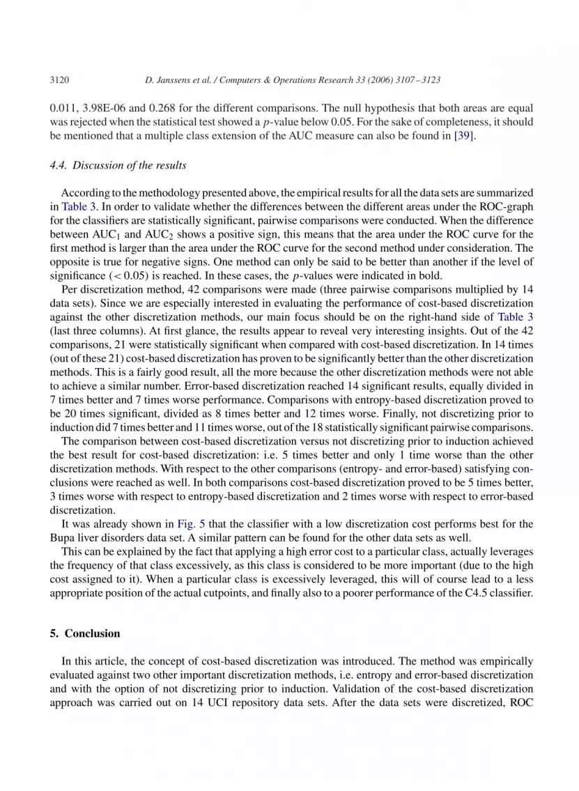
0.011, 3.98E-06 and 0.268 for the different comparisons. The null hypothesis that both areas are equalwas rejected when the statistical test showed a p-value below 0.05. For the sake of completeness, it shouldbe mentioned that a multiple class extension of the AUC measure can also be found in [39].

4.4. Discussion of the results

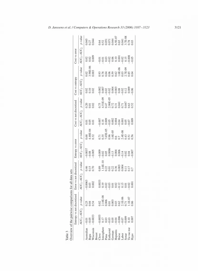
According to the methodology presented above, the empirical results for all the data sets are summarizedin Table 3. In order to validate whether the differences between the different areas under the ROC-graphfor the classifiers are statistically significant, pairwise comparisons were conducted. When the differencebetween AUC1 and AUC2 shows a positive sign, this means that the area under the ROC curve for thefirst method is larger than the area under the ROC curve for the second method under consideration. Theopposite is true for negative signs. One method can only be said to be better than another if the level ofsignificance (< 0.05) is reached. In these cases, the p-values were indicated in bold.

Per discretization method, 42 comparisons were made (three pairwise comparisons multiplied by 14data sets). Since we are especially interested in evaluating the performance of cost-based discretizationagainst the other discretization methods, our main focus should be on the right-hand side of Table 3(last three columns). At first glance, the results appear to reveal very interesting insights. Out of the 42comparisons, 21 were statistically significant when compared with cost-based discretization. In 14 times(out of these 21) cost-based discretization has proven to be significantly better than the other discretizationmethods. This is a fairly good result, all the more because the other discretization methods were not ableto achieve a similar number. Error-based discretization reached 14 significant results, equally divided in7 times better and 7 times worse performance. Comparisons with entropy-based discretization proved tobe 20 times significant, divided as 8 times better and 12 times worse. Finally, not discretizing prior toinduction did 7 times better and 11 times worse, out of the 18 statistically significant pairwise comparisons.

The comparison between cost-based discretization versus not discretizing prior to induction achievedthe best result for cost-based discretization: i.e. 5 times better and only 1 time worse than the otherdiscretization methods. With respect to the other comparisons (entropy- and error-based) satisfying con-clusions were reached as well. In both comparisons cost-based discretization proved to be 5 times better,3 times worse with respect to entropy-based discretization and 2 times worse with respect to error-baseddiscretization.

It was already shown in Fig. 5 that the classifier with a low discretization cost performs best for theBupa liver disorders data set. A similar pattern can be found for the other data sets as well.

This can be explained by the fact that applying a high error cost to a particular class, actually leveragesthe frequency of that class excessively, as this class is considered to be more important (due to the highcost assigned to it). When a particular class is excessively leveraged, this will of course lead to a lessappropriate position of the actual cutpoints, and finally also to a poorer performance of the C4.5 classifier.

5. Conclusion

In this article, the concept of cost-based discretization was introduced. The method was empiricallyevaluated against two other important discretization methods, i.e. entropy and error-based discretizationand with the option of not discretizing prior to induction. Validation of the cost-based discretizationapproach was carried out on 14 UCI repository data sets. After the data sets were discretized, ROC


Tabl

e3

Ove

rvie

wof

the

pair

wis

eco

mpa

riso

nsfo

ral

ldat

ase

tsE

ntro

pyvs

notd

iscr

etiz

edE

rror

vsno

tdis

cret

ized

Ent

ropy

vser

ror

Cos

tvs

notd

iscr

etiz

edC

ostv

sen

trop

yC

ostv

ser

ror

AU

C1–A

UC

2p

-val

ueA

UC

1–A

UC

2p

-val

ueA

UC

1–A

UC

2p

-val

ueA

UC

1–A

UC

2p

-val

ueA

UC

1–A

UC

2p

-val

ueA

UC

1–A

UC

2p

-val

ue

Aus

tral

ian

−0.0

10.

25−0

.006

30.

46−0

.003

70.

680.

010.

200.

020.

020.

020.

045

Bup

a−0

.05

0.04

0.03

0.15

−0.0

84.

48E

-04

0.05

0.01

0.10

3.98

E-0

60.

020.

27W

isco

nsin

−0.0

033

0.54

0.00

20.

70−0

.005

0.32

0.01

0.02

0.02

0.00

30.

009

0.04

4B

reas

tC

leve

−0.0

055

0.82

0.00

330.

89−0

.009

0.71

−0.0

070.

75−0

.002

0.93

−0.0

10.

64Io

nosp

here

0.17

2.14

E-0

80.

191.

14E

-10

−0.0

20.

350.

184.

51E

-09

0.00

70.

78−0

.01

0.52

Pim

a0.

030.

006

−0.0

20.

220.

057.

65E

-05

0.00

90.

47−0

.02

0.04

0.03

0.05

1E

uthy

roid

−0.0

30.

01−0

.03

0.01

0.00

060.

96−0

.05

2.06

E-0

5−0

.02

0.06

−0.0

20.

071

Ger

man

0.05

0.00

30.

010.

22−0

.13

1.6E

-05

0.00

20.

720.

004

0.59

0.06

0.04

4H

epat

itis

−0.0

40.

030.

020.

360.

004

0.6

0.00

40.

31−0

.003

0.62

0.10

6.5E

-07

Hor

se−0

.006

0.62

−0.1

20.

003

0.00

60.

7−0

.04

0.04

10.

081.

6E-0

60.

001

0.65

Lab

or−0

.07

2.1E

-06

0.15

0.00

4−0

.14

2.4E

-08

0.00

10.

71−0

.02

0.03

−0.0

20.

041

Sona

r−0

.009

0.71

0.01

0.11

−0.0

20.

430.

050.

047

0.12

2.7E

-09

0.15

3.7E

-08

Tic

-tac

-toe

0.10

1.1E

-07

−0.0

20.

170.

040.

51−0

.07

0.63

0.00

90.

85−0

.008

0.78

Hyp

o0.

007

0.86

0.00

10.

7−0

.007

0.56

0.00

90.

52−0

.06

0.04

−0.0

50.

03


analysis was used to evaluate the performance of the different classification trees. To be able to make avalid assessment which method performs best, the area under the ROC curve and p-values were used ascriteria to reflect the performance of the classifier.

Although cost-based discretization did not dominate other discretization methods all along the line, theempirical results showed that for those data sets that reached statistically significant results, cost-baseddiscretization achieved very satisfactory results when compared to entropy and error-based discretization.Results also showed that the best results for the cost-based discretization method are usually obtainedwith relatively low discretization costs.

On the other hand it has to be noted that at most half of the pairwise comparisons were significant. Thisindicates that there are still opportunities for future research in improving the effect that cost-based andother discretization methods can have on the final accuracy after induction. Also further research is stillneeded to better understand why it is not always the same discretization cost parameter that performs bestover the data sets. The fact that class distributions differ significantly for the data sets and that differentpatterns may be incorporated in the data sets are plausible explanations but further research should stillvalidate this.Also, as mentioned above, alternative methods or heuristics for cost-based discretization needto be considered in the future. For instance, adapting instance weighting and then subsequently applyingexisting error-based discretization methods may be one possibility. Or, alternatively, reformulating theproblem as a dynamic instead of an integer programming approach, is another interesting avenue forfuture research.

References

[1] Workshop on Cost-Sensitive Learning. In conjunction with the Seventeenth International Conference on Machine Learning,ICML-2000, Stanford University, June 29–July 2, 2000.

[2] Lee C, Shin D-G. A context-sensitive discretization of numeric attributes for classification learning. In: Proceedings of theeleventh European conference on artificial intelligence. Amsterdam: Wiley; 1994. p. 428–32.

[3] Fayyad U, Irani K. Multi-interval discretization of continuous valued attributes for classification learning. In: Proceedingsof the 13th international joint conference on artificial intelligence. San Francisco: Morgan Kaufmann; 1993. p. 1022–7.

[4] Pfahringer B. Compression-based discretization of continuous attributes. In: Proceedings of the 12th internationalconference on machine learning. San Francisco: Morgan Kaufmann; 1995. p. 456–63.

[5] Fulton T, Kasif S, Salzberg S. Efficient algorithms for finding multi-way splits for decision trees. In: Proceedings of the12th international conference on machine learning. San Francisco: Morgan Kaufmann; 1995. p. 244–51.

[6] Bay SD. Multivariate discretization for set mining. Knowledge and Information Systems 2001;3(4):491–512.[7] Elomaa T, Rousu J. Preprocessing opportunities in optimal numerical range partitioning. In: Proceedings of the first IEEE

international conference on data mining. Silver Spring, MD: IEEE Computer Society Press; 2001. p. 115–22.[8] Cantú-Paz E. Supervised and unsupervised discretization methods for evolutionary algorithms. In: Proceedings genetic

and evolutionary computation conference 2001. San Francisco: Morgan Kaufmann; 2001. p. 213–6.[9] Quinlan JR. C4.5: Programs for machine learning. Los Altos: Morgan Kaufmann; 1993.

[10] Breiman L, Friedman JH, Olshen RA, Stone CJ. Classification and regression trees. Belmont, CA: Wadsworth; 1984.[11] Friedman N, Goldszmidt M. Discretizing continuous attributes while learning bayesian networks. In: Proceeding of the

13th international conference on machine learning. Los Altos, CA: Morgan Kaufmann; 1996. p. 157–65.[12] Dougherty J, Kohavi R, Sahami M. Supervised and unsupervised discretization of continuous features. In: Proceedings of

the 12th international conference on machine learning. San Francisco: Morgan Kaufmann; 1995. p. 194–202.[13] Wettschereck D, Aha D, Mohri TA. A review and empirical evaluation of feature weighting methods for a class of lazy

learning algorithms. Artificial Intelligence Review 1997;11(1/5):273–314.[14] Blockeel H, Raedt LD. Lookahead and discretization in ILP. In: Proceedings of the seventh international workshop on

inductive logic programming, Lecture Notes in Artificial Intelligence, vol. 1297, Springer, Berlin, 1997, p. 77–84.


[15] Hekanaho J. DOGMA: a GA-based relational learner. Proceeding of the eighth international conference on inductive logicprogramming (ILP-98), Lecture Notes in Artificial Intelligence, vol. 1446. Berlin: Springer; 1998. p. 205–14.

[16] Kohavi R, Sahami M. Error-based and entropy-based discretization of continuous features. In: Proceedings of the secondinternational conference on knowledge & data mining. Menlo Park: AAAI Press; 1996. p. 114–9.

[17] Catlett J. On changing continuous attributes into ordered discrete attributes. In: Proceedings of the fifth European workingsession on learning. Berlin: Springer; 1991. p. 164–78.

[18] Blake CL, Merz CJ. UCI repository of machine learning databases [http://www.ics.uci.edu/∼mlearn/MLRepository.html].Irvine, CA: University of California, Department of Information and Computer Science, 1998.

[19] Maass W. Efficient agnostic PAC-learning with simple hypotheses. In: Proceedings of the seventh annual ACM conferenceon computational learning theory. New York: ACM Press; 1994. p. 67–75.

[20] Elomaa T, Rousu J. Fast minimum error discretization. In: Proceedings of the 19th international conference on machinelearning. Los Altos, CA: Morgan Kaufmann; 2002. p. 131–8.

[21] Rissanen J. Stochastic complexity in statistical inquiry. Singapore: World Scientific; 1989.[22] Chmielewski MR, Grzymala-Busse JW. Global discretization of continuous attributes as preprocessing for machine

learning. In Third international workshop on rough sets and soft computing, 1994. p. 294–301.[23] Holte R. Very simple classification rules perform well on most commonly used datasets. Machine Learning 1993;11:

63–90.[24] Van de Merckt T. Decision trees in numerical attributes spaces. In: Proceedings of the 13th international joint conference

on artificial intelligence. Los Altos, CA: Morgan Kaufmann; 1993. p. 1016–21.[25] Kerber R. Chimerge: discretization of numeric attributes. In: Proceedings of the 10th national conference on artificial

intelligence. Cambridge, MA: MIT Press; 1992. p. 123–8.[26] Fayyad U, Irani K. On the handling of continuous-valued attributes in decision tree generation. Machine Learning 1992;8:87

–102.[27] Elomaa T, Rousu J. Generalizing boundary points. In: Proceedings of the 17th national conference on artificial intelligence,

AAAI. Cambridge, MA: MIT Press; 2000. p. 570–6.[28] Elomaa T, Rousu J. General and efficient multisplitting of numerical attributes. Machine Learning 1999;36(3):201–44.[29] Elomaa T, Rousu J. Efficient multisplitting revisited: optima-preserving elimination of partition candidates. Data Mining

and Knowledge Discovery 2004;8(2):97–126.[30] Hillier F, Lieberman G. Introduction to operations research. 6 ed., New York: McGraw Hill; 1995.[31] Ting KM. Inducing cost-sensitive trees via instance weighting. In: Principles of data mining and knowledge discovery

(PKDD’98). Berlin: Springer; 1998. p. 139–47.[32] Elomaa T, Rousu J. Finding optimal multi-splits for numerical attributes in decision tree learning. Technical Report,

NC-TR-96-041, University of Helsinki, 1996.[33] Quinlan J. Improved use of continuous attributes in C4.5. Journal of Artificial Intelligence Research 1996;4:77–90.[34] Bradley AP. The use of the area under the ROC curve in the evaluation of machine learning algorithms. Pattern Recognition

1997;30(7):1145–59.[35] Ling CX, Huang J, Zhang H.AUC: a statistically consistent and more discriminating measure than accuracy. In: Proceedings

of 18th international conference on artificial intelligence (IJCAI-2003) , 2003. p. 329–41.[36] Provost F, Fawcett T. Analysis and visualization of classifier performance: comparison under imprecise class and cost

distributions. In: Proceedings of the third international conference on knowledge discovery and data mining. Menlo Park:AAAI Press; 1997. p. 43–8.

[37] Hanley JA, McNeil BJ. A method of comparing the areas under receiver operating characteristic curves derived from thesame cases. Radiology 1983;148:839–43.

[38] Kendall MG. A new measure of rank correlation. Biometrika 1938;30:81–92.[39] Hand DJ, Till RJ. A simple generalisation of the area under the ROC curve for multiple class classification problems.

Machine Learning 2001;45:171–86.

http://www.ics.uci.edu/~mlearn/MLRepository.html

evaluating the performance of cost-based discretization versus entropy- and error-based...

Documents