mixed equations - numerical examples of pde discretization
TRANSCRIPT
Classification of PDE Mixed equations Methods for forward marching in time Examples Summary
Mixed EquationsNumerical examples of PDE discretization
F. Durastante1
1Dipartimento di Scienza e Alta TecnologiaUniversità dell’Insubria
1 December 2014
Classification of PDE Mixed equations Methods for forward marching in time Examples Summary
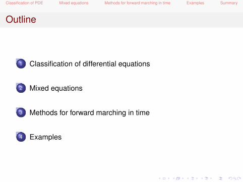
Outline
1 Classification of differential equations
2 Mixed equations
3 Methods for forward marching in time
4 Examples
Classification of PDE Mixed equations Methods for forward marching in time Examples Summary
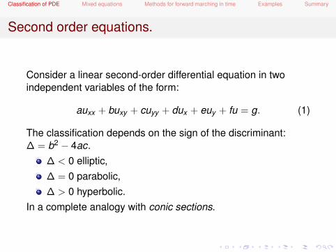
Second order equations.
Consider a linear second-order differential equation in twoindependent variables of the form:
auxx + buxy + cuyy + dux + euy + fu = g. (1)
The classification depends on the sign of the discriminant:∆ = b2 − 4ac.
∆ < 0 elliptic,∆ = 0 parabolic,∆ > 0 hyperbolic.
In a complete analogy with conic sections.
Classification of PDE Mixed equations Methods for forward marching in time Examples Summary
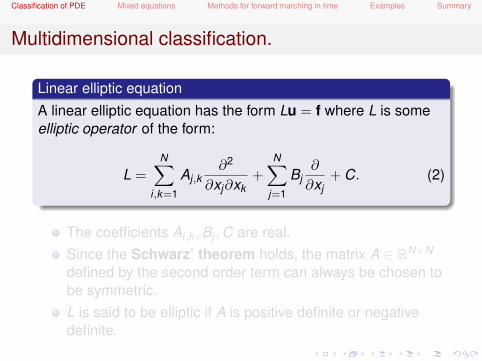
Multidimensional classification.
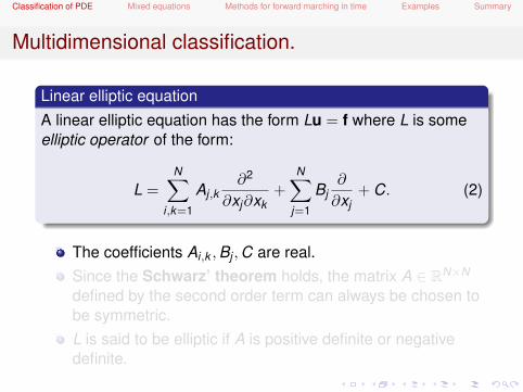
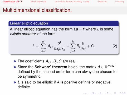
Linear elliptic equationA linear elliptic equation has the form Lu = f where L is someelliptic operator of the form:
L =N∑
i,k=1
Aj,k∂2
∂xj∂xk+
N∑j=1
Bj∂
∂xj+ C. (2)
The coefficients Ai,k ,Bj ,C are real.Since the Schwarz’ theorem holds, the matrix A ∈ RN×N
defined by the second order term can always be chosen tobe symmetric.L is said to be elliptic if A is positive definite or negativedefinite.
Classification of PDE Mixed equations Methods for forward marching in time Examples Summary
Multidimensional classification.
Linear elliptic equationA linear elliptic equation has the form Lu = f where L is someelliptic operator of the form:
L =N∑
i,k=1
Aj,k∂2
∂xj∂xk+
N∑j=1
Bj∂
∂xj+ C. (2)
The coefficients Ai,k ,Bj ,C are real.Since the Schwarz’ theorem holds, the matrix A ∈ RN×N
defined by the second order term can always be chosen tobe symmetric.L is said to be elliptic if A is positive definite or negativedefinite.
Classification of PDE Mixed equations Methods for forward marching in time Examples Summary
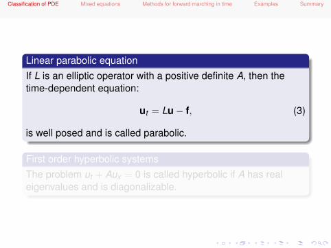
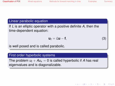
Linear parabolic equationIf L is an elliptic operator with a positive definite A, then thetime-dependent equation:
ut = Lu− f, (3)
is well posed and is called parabolic.
First order hyperbolic systemsThe problem ut + Aux = 0 is called hyperbolic if A has realeigenvalues and is diagonalizable.
Classification of PDE Mixed equations Methods for forward marching in time Examples Summary
Mixed equations
Actually several processes may be happening simultaneously,and the PDE will not be a pure equation of any of the previoustype.We then consider problem of the form:
ut =M∑
i=1
Ai(u) (4)
where Ai can be both a function or a differential operators,possibly nonlinear.
Classification of PDE Mixed equations Methods for forward marching in time Examples Summary
An (incomplete) set of examples.
Reaction-Diffusion equationsEquations of the form:
ut = κ∇2u + R(u), (5)
where κ is the diagonal matrix of the diffusion coefficients andR(u) is the reaction term (typically nonlinear).
The term R(U) might or might not be stiff. This couldsuggest using mixed approach for solving this equations.The diffusive term is intrinsically stiff and requiresappropriate methods.
Classification of PDE Mixed equations Methods for forward marching in time Examples Summary
An (incomplete) set of examples.
Advection-Diffusion equationsEquations of the form:
ut + a∇u = κ∇2u. (6)
where κ is the diagonal matrix of the diffusion coefficients and ais the transport velocity.
The advection term can be handled explicitly.The diffusive term is intrinsically stiff and requiresappropriate methods.
Classification of PDE Mixed equations Methods for forward marching in time Examples Summary
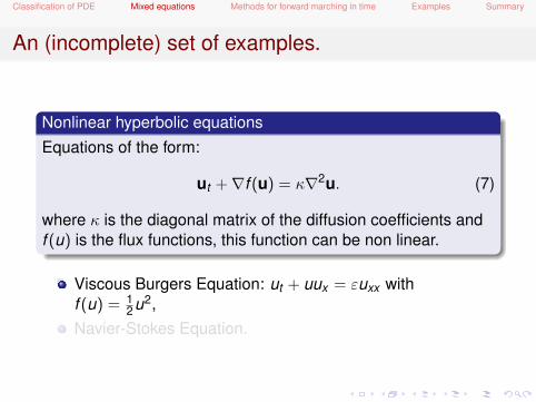
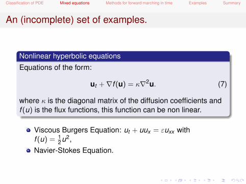
An (incomplete) set of examples.
Nonlinear hyperbolic equationsEquations of the form:
ut +∇f (u) = κ∇2u. (7)
where κ is the diagonal matrix of the diffusion coefficients andf (u) is the flux functions, this function can be non linear.
Viscous Burgers Equation: ut + uux = εuxx withf (u) = 1
2u2,Navier-Stokes Equation.
Classification of PDE Mixed equations Methods for forward marching in time Examples Summary
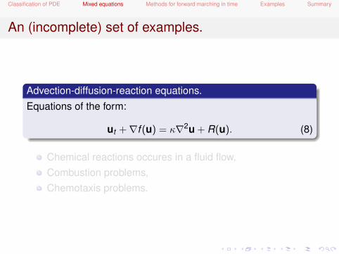
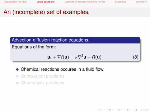
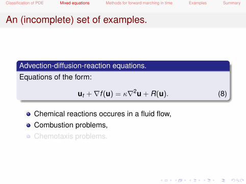
An (incomplete) set of examples.
Advection-diffusion-reaction equations.Equations of the form:
ut +∇f (u) = κ∇2u + R(u). (8)
Chemical reactions occures in a fluid flow,Combustion problems,Chemotaxis problems.
Classification of PDE Mixed equations Methods for forward marching in time Examples Summary
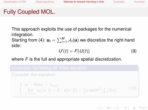
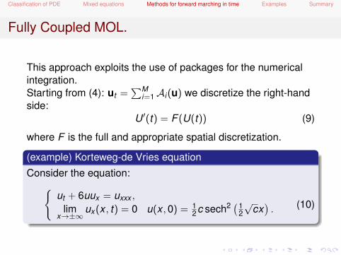
Fully Coupled MOL.
This approach exploits the use of packages for the numericalintegration.Starting from (4): ut =
∑Mi=1Ai(u) we discretize the right-hand
side:U ′(t) = F (U(t)) (9)
where F is the full and appropriate spatial discretization.
(example) Korteweg-de Vries equation
Consider the equation:ut + 6uux = uxxx ,
limx→±∞
ux (x , t) = 0 u(x ,0) = 12c sech2 (1
2√
cx). (10)
Classification of PDE Mixed equations Methods for forward marching in time Examples Summary
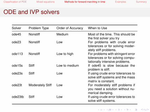
ODE and IVP solvers
Solver Problem Type Order of Accuracy When to Use
ode45 Nonstiff Medium Most of the time. This should bethe first solver you try
ode23 Nonstiff Low For problems with crude errortolerances or for solving moder-ately stiff problems.
ode113 Nonstiff Low to high For problems with stringent errortolerances or for solving compu-tationally intensive problems.
ode15s Stiff Low to medium If ode45 is slow because theproblem is stiff.
ode23s Stiff Low If using crude error tolerances tosolve stiff systems and the massmatrix is constant.
ode23t Moderately Stiff Low For moderately stiff problems ifyou need a solution without nu-merical damping.
ode23tb Stiff Low If using crude error tolerances tosolve stiff systems.
Classification of PDE Mixed equations Methods for forward marching in time Examples Summary
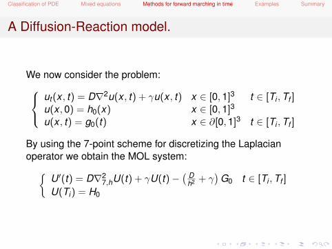
A Diffusion-Reaction model.
We now consider the problem:ut (x , t) = D∇2u(x , t) + γu(x , t) x ∈ [0,1]3 t ∈ [Ti ,Tf ]u(x ,0) = h0(x) x ∈ [0,1]3
u(x , t) = g0(t) x ∈ ∂[0,1]3 t ∈ [Ti ,Tf ]
By using the 7-point scheme for discretizing the Laplacianoperator we obtain the MOL system:
U ′(t) = D∇27,hU(t) + γU(t)−
( Dh2 + γ
)G0 t ∈ [Ti ,Tf ]
U(Ti) = H0
Classification of PDE Mixed equations Methods for forward marching in time Examples Summary
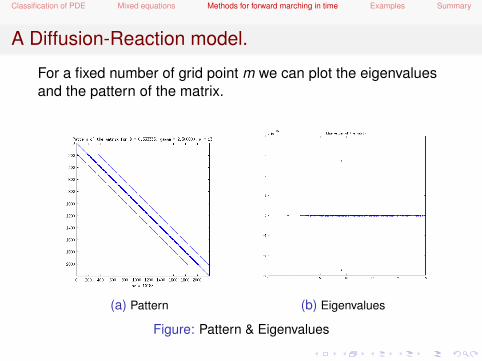
A Diffusion-Reaction model.
For a fixed number of grid point m we can plot the eigenvaluesand the pattern of the matrix.
(a) Pattern (b) Eigenvalues
Figure: Pattern & Eigenvalues
Classification of PDE Mixed equations Methods for forward marching in time Examples Summary
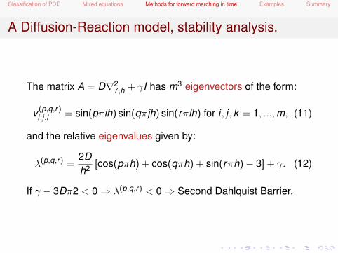
A Diffusion-Reaction model, stability analysis.
The matrix A = D∇27,h + γI has m3 eigenvectors of the form:
v (p,q,r)i,j,l = sin(pπih) sin(qπjh) sin(rπlh) for i , j , k = 1, ...,m, (11)
and the relative eigenvalues given by:
λ(p,q,r) =2Dh2 [cos(pπh) + cos(qπh) + sin(rπh)− 3] + γ. (12)
If γ − 3Dπ2 < 0⇒ λ(p,q,r) < 0⇒ Second Dahlquist Barrier.
Classification of PDE Mixed equations Methods for forward marching in time Examples Summary
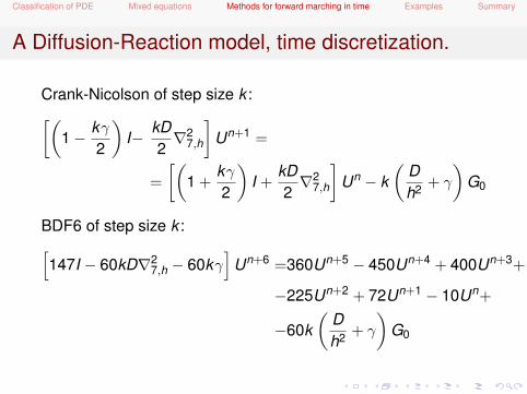
A Diffusion-Reaction model, time discretization.
Crank-Nicolson of step size k :[(1− kγ
2
)I− kD
2∇2
7,h
]Un+1 =
=
[(1 +
kγ2
)I +
kD2∇2
7,h
]Un − k
(Dh2 + γ
)G0
BDF6 of step size k :[147I − 60kD∇2
7,h − 60kγ]
Un+6 =360Un+5 − 450Un+4 + 400Un+3+
−225Un+2 + 72Un+1 − 10Un+
−60k(
Dh2 + γ
)G0
Classification of PDE Mixed equations Methods for forward marching in time Examples Summary
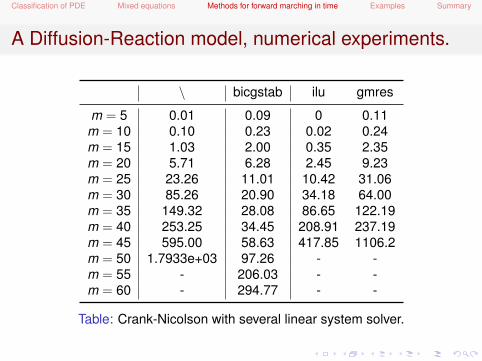
A Diffusion-Reaction model, numerical experiments.
\ bicgstab ilu gmres
m = 5 0.01 0.09 0 0.11m = 10 0.10 0.23 0.02 0.24m = 15 1.03 2.00 0.35 2.35m = 20 5.71 6.28 2.45 9.23m = 25 23.26 11.01 10.42 31.06m = 30 85.26 20.90 34.18 64.00m = 35 149.32 28.08 86.65 122.19m = 40 253.25 34.45 208.91 237.19m = 45 595.00 58.63 417.85 1106.2m = 50 1.7933e+03 97.26 - -m = 55 - 206.03 - -m = 60 - 294.77 - -
Table: Crank-Nicolson with several linear system solver.
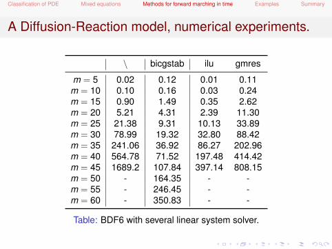
Classification of PDE Mixed equations Methods for forward marching in time Examples Summary
A Diffusion-Reaction model, numerical experiments.
\ bicgstab ilu gmres
m = 5 0.02 0.12 0.01 0.11m = 10 0.10 0.16 0.03 0.24m = 15 0.90 1.49 0.35 2.62m = 20 5.21 4.31 2.39 11.30m = 25 21.38 9.31 10.13 33.89m = 30 78.99 19.32 32.80 88.42m = 35 241.06 36.92 86.27 202.96m = 40 564.78 71.52 197.48 414.42m = 45 1689.2 107.84 397.14 808.15m = 50 - 164.35 - -m = 55 - 246.45 - -m = 60 - 350.83 - -
Table: BDF6 with several linear system solver.
Classification of PDE Mixed equations Methods for forward marching in time Examples Summary
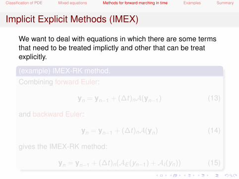
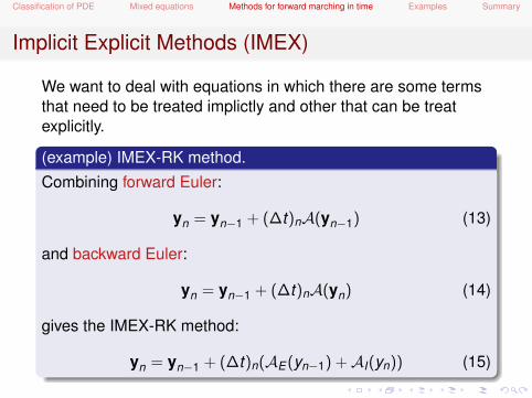
Implicit Explicit Methods (IMEX)
We want to deal with equations in which there are some termsthat need to be treated implictly and other that can be treatexplicitly.
(example) IMEX-RK method.Combining forward Euler:
yn = yn−1 + (∆t)nA(yn−1) (13)
and backward Euler:
yn = yn−1 + (∆t)nA(yn) (14)
gives the IMEX-RK method:
yn = yn−1 + (∆t)n(AE (yn−1) +AI(yn)) (15)
Classification of PDE Mixed equations Methods for forward marching in time Examples Summary
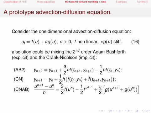
A prototype advection-diffusion equation.
Consider the one dimensional advection-diffusion equation:
ut = f (u) + νg(u), ν > 0, f non linear, νg(u) stiff. (16)
a solution could be mixing the 2nd order Adam-Bashforth(explicit) and the Crank-Nicolson (implicit):
(AB2) yn+2 = yn+1 +32
hf (tn+1, yn+1)− 12
hf (tn, yn);
(CN) yn+1 = yn +12
h (f (tn, yn) + f (tn+1, yn+1)) ;
(CNAB)un+1 − un
h=
32
f (un)− 12
f un−1+η
2
[g(un+1 + g(un))
]
Classification of PDE Mixed equations Methods for forward marching in time Examples Summary
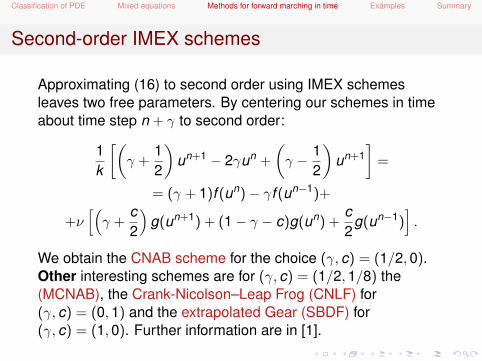
Second-order IMEX schemes
Approximating (16) to second order using IMEX schemesleaves two free parameters. By centering our schemes in timeabout time step n + γ to second order:
1k
[(γ +
12
)un+1 − 2γun +
(γ − 1
2
)un+1
]=
= (γ + 1)f (un)− γf (un−1)+
+ν[(γ +
c2
)g(un+1) + (1− γ − c)g(un) +
c2
g(un−1)].
We obtain the CNAB scheme for the choice (γ, c) = (1/2,0).Other interesting schemes are for (γ, c) = (1/2,1/8) the(MCNAB), the Crank-Nicolson–Leap Frog (CNLF) for(γ, c) = (0,1) and the extrapolated Gear (SBDF) for(γ, c) = (1,0). Further information are in [1].
Classification of PDE Mixed equations Methods for forward marching in time Examples Summary
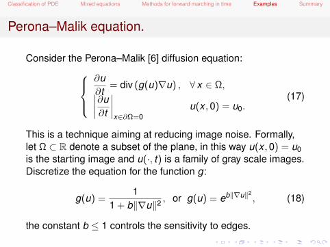
Perona–Malik equation.
Consider the Perona–Malik [6] diffusion equation:∂u∂t
= div (g(u)∇u) , ∀ x ∈ Ω,∣∣∣∣∂u∂t
∣∣∣∣x∈∂Ω=0
u(x ,0) = u0.(17)
This is a technique aiming at reducing image noise. Formally,let Ω ⊂ R denote a subset of the plane, in this way u(x ,0) = u0is the starting image and u(·, t) is a family of gray scale images.Discretize the equation for the function g:
g(u) =1
1 + b‖∇u‖2, or g(u) = eb‖∇u‖2
, (18)
the constant b ≤ 1 controls the sensitivity to edges.
Classification of PDE Mixed equations Methods for forward marching in time Examples Summary
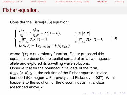
Fisher equation.
Consider the Fisher[4, 5] equation:∂u∂t
= D∂2u∂x2 + ru(1− u), x ∈ [a,b],
limx→−∞
u(x , t) = 1, limx→+∞
u(x , t) = 0,
u(x ,0) = 1χ(−∞,a) + f (x)χ(a,b).
(19)
where f (x) is an arbitrary function. Fisher proposed thisequation to describe the spatial spread of an advantageousallele and explored its travelling wave solutions.Observe that for the bounded initial data of the form,0 ≤ u(x ,0) ≤ 1, the solution of the Fisher equation is alsobounded (Kolmogorov, Petrovsky, and Piskunov - 1937). Whathappens to the solution for the discontinuous initial data(described above)?
Classification of PDE Mixed equations Methods for forward marching in time Examples Summary
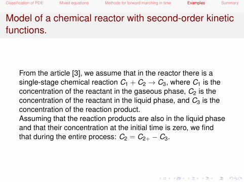
Model of a chemical reactor with second-order kineticfunctions.
From the article [3], we assume that in the reactor there is asingle-stage chemical reaction C1 + C2 → C3, where C1 is theconcentration of the reactant in the gaseous phase, C2 is theconcentration of the reactant in the liquid phase, and C3 is theconcentration of the reaction product.Assuming that the reaction products are also in the liquid phaseand that their concentration at the initial time is zero, we findthat during the entire process: C2 = C2+ − C3.
Classification of PDE Mixed equations Methods for forward marching in time Examples Summary
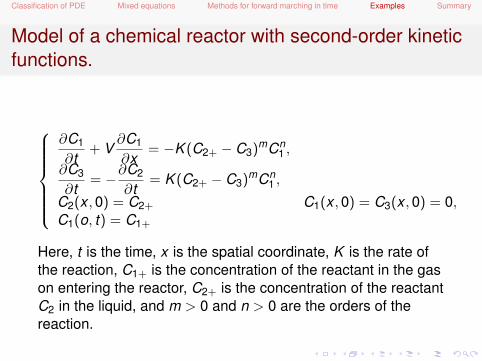
Model of a chemical reactor with second-order kineticfunctions.
∂C1
∂t+ V
∂C1
∂x= −K (C2+ − C3)mCn
1 ,
∂C3
∂t= −∂C2
∂t= K (C2+ − C3)mCn
1 ,
C2(x ,0) = C2+ C1(x ,0) = C3(x ,0) = 0,C1(o, t) = C1+
Here, t is the time, x is the spatial coordinate, K is the rate ofthe reaction, C1+ is the concentration of the reactant in the gason entering the reactor, C2+ is the concentration of the reactantC2 in the liquid, and m > 0 and n > 0 are the orders of thereaction.
Classification of PDE Mixed equations Methods for forward marching in time Examples Summary
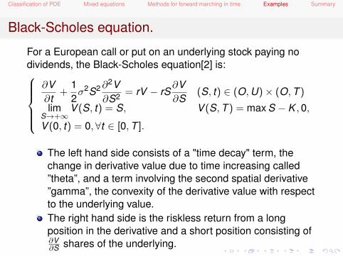
Black-Scholes equation.
For a European call or put on an underlying stock paying nodividends, the Black-Scholes equation[2] is:
∂V∂t
+12σ2S2∂
2V∂S2 = rV − rS
∂V∂S
(S, t) ∈ (O,U)× (O,T )
limS→+∞
V (S, t) = S, V (S,T ) = max S − K ,0,
V (0, t) = 0,∀t ∈ [0,T ].
The left hand side consists of a "time decay" term, thechange in derivative value due to time increasing called”theta”, and a term involving the second spatial derivative”gamma”, the convexity of the derivative value with respectto the underlying value.The right hand side is the riskless return from a longposition in the derivative and a short position consisting of∂V∂S shares of the underlying.
Classification of PDE Mixed equations Methods for forward marching in time Examples Summary
Black-Scholes equation.
In this way we have that V is the price of the option as afunction of stock price S and time t , r is the risk-free interestrate, and σ is the volatility of the stock.
Classification of PDE Mixed equations Methods for forward marching in time Examples Summary
General scheme for the project
A scheme for the project:Write an introduction to the model.Discuss the spatial discretization and then apply the MOLapproach (maybe with different time integrator).Discuss the stability of the system.Full discretize the system with various time integrator.Try different combinations of linear solvers andpreconditioners.Discuss the numerical results.
Classification of PDE Mixed equations Methods for forward marching in time Examples Summary
Bibliography I
Uri M Ascher, Steven J Ruuth, and Brian TR Wetton.Implicit-explicit methods for time-dependent partial differentialequations.SIAM Journal on Numerical Analysis, 32(3):797–823, 1995.
Fischer Black and Myron Scholes.The pricing of options and corporate liabilities.The journal of political economy, pages 637–654, 1973.
V. S. Berman; L. A. Galin; O. M. Churmaev.Analysis of a simple model of a bubble-liquid reactor.Fluid Dynamics, 14, 09-10 1979.
Ronald Aylmer Fisher.The wave of advance of advantageous genes.Annals of Eugenics, 7(4):355–369, 1937.
Classification of PDE Mixed equations Methods for forward marching in time Examples Summary
Bibliography II
Ronald Aylmer Fisher.
The genetical theory of natural selection.
1958.
Pietro Perona and Jitendra Malik.
Scale-space and edge detection using anisotropic diffusion.
Pattern Analysis and Machine Intelligence, IEEE Transactionson, 12(7):629–639, 1990.