Mesh Algorithms for PDE with Sieve I: MeshDistribution

Matthew G. KnepleyComputation InstituteUniversity of Chicago

Chicago, IL 60637

Dmitry A. KarpeevMathematics and Computer Science Division

Argonne National LaboratoryArgonne, IL 60439

August 30, 2009

AbstractWe have developed a new programming framework, called Sieve,

to support parallel numerical PDE1 algorithms operating over dis-tributed meshes. We have also developed a reference implementationof Sieve in C++ as a library of generic algorithms operating on dis-tributed containers conforming to the Sieve interface. Sieve makes in-stances of the incidence relation, or arrows, the conceptual first-classobjects represented in the containers. Further, generic algorithms act-ing on this arrow container are systematically used to provide naturalgeometric operations on the topology and also, through duality, onthe data. Finally, coverings and duality are used to encode not onlyindividual meshes, but all types of hierarchies underlying PDE datastructures, including multigrid and mesh partitions.

In order to demonstrate the usefulness of the framework, we showhow the mesh partition data can be represented and manipulated us-ing the same fundamental mechanisms used to represent meshes. We

1Partial differential equation(s).

1

arX

iv:0

908.

4427

v1 [

cs.C

E]

30

Aug

200

9

present the complete description of an algorithm to encode a mesh par-tition and then distribute a mesh, which is independent of the meshdimension, element shape, or embedding. Moreover, data associatedwith the mesh can be similarly distributed with exactly the same al-gorithm. The use of a high level of abstraction within the Sieve leadsto several benefits in terms of code reuse, simplicity, and extensibility.We discuss these benefits and compare our approach to other existingmesh libraries.

1 Introduction

Numerical PDE codes frequently comprise of two uneasily coexisting pieces:the mesh, describing the topology and geometry of the domain, and the func-tional data attached to the mesh representing the discretized fields and equa-tions. The mesh data structure typically reflects the representation used bythe mesh generator and carries the embedded geometic information. Whilethis arrangement is natural from the point of view of mesh generation andexists in the best of such packages (e.g., [17]), it is frequently foreign to theprocess of solving equations on the generated mesh.

At the same time, the functional data closely reflect the linear algebraicstructure of the computational kernels ultimately used to solve the equations;here the natural geometric structure of the equations, which reflects the meshconnectivity in the coupling between the degrees of freedom, is sacrificed tothe rigid constraints of the solver. In particular, the most natural geometricoperation of a restriction of a field to a local neighborhood entails tediousand error-prone index manipulation.

In response to this state of affairs a number of efforts arose addressing thefundamental issues of interaction between the topology, the functional dataand algorithms. We note the MOAB project [20, 19, 8] and the TSTT/ITAPSSciDAC projects [8, 16, 3], the libMesh project [6], the GrAL project [4], toname just a few. Sieve shares many features with these projects, but GrALis the closest to it in spirit. Although each of these projects addresses someof the issues outlined above, we feel that there is room for another approach.

Our Sieve framework, is a collection of interfaces and algorithms for ma-nipulating geometric data. The design may be summarized by consideringthree constructions. First, data in Sieve are indexed by the underlying ge-ometric elements, such as mesh cells, rather than by some artificial global

2

order. Further, the local traversal of the data is based on the connectivity ofthe geometric elements. For example, Sieve provides operations that, givena mesh cell, traverse all the data on its interior, its boundary, or its closure.Typical operations on a Sieve are shown in Table 1 and described in greaterdetail in Section 2.1. In the table, topological mesh elements, such as ver-tices, edges, and so on, are refered to as abstract points 2, and the adjacencyrelation between two points, such as an edge and its vertex, is refered to ascovering : an edge is coverted by its end vertices. Notice that exactly thesame operation is used to obtain edges adjacent to a face as faces adjacentto a cell, without even a lurking dimension parameter. This is the key toenabling dimension-independent programming for PDE algorithms.

Second, the global topology is divided into a chain of local topologies withan overlap structure relating them to each other. The overlap is encodedusing the Sieve data structure again, this time containing arrows relatingpoints in different local topologies. The data values over each local piece aremanipulated using the local connectivity, and each local piece may associatedifferent data to the same global element. The crucial ingredient here is theoperation of assembling the chain of local data collections into a consistentwhole over the global topology.

Third, the covering arrows can carry additional information, controllingthe way in which the data from the covering points are assembled onto thecovered points. For example, orientation information can be encoded onthe arrows to dictate an order for data returned over an element closure.More sophisticated operations are also possible, such as linear combinationswhich enable coordinate transformations, or the projection and interpolationnecessary for multigrid algorithms. This is the central motivation behind thearrow-centric interface.

Emphasis on the covering idea stems directly from the cell complex con-struction in algebraic topology. We have abstracted it along the lines ofcategory theory, with its emphasis on arrows, or morphisms, as the organiz-ing principle. The analogy runs deeper, however, because in PDE applica-tions meshes do not exist for their own sake, but to support geometricallystructured information. The geometric structure of these data manifests it-self through duality between topogical operations, such as closure of a meshelement, and analytical operations, such as the restriction of a field to a

2Our points correspond to geometric entities in some other approaches like MOAB orITAPS

3

closed neighborhood of the element. Formally this can be seen as a reversalof arrows in a suitable category. At the practical level, this motivates thearrow-centric point of view, which allows us to load the arrows with the data(e.g., coordinate transformation parameters) making the dualization betweencovering and restriction possible.

The arrow-centric point of view also distinguishes our approach from sim-ilar projects such as [4]. In addition, it is different from the concept of a flex-ible database of geometric entities underlying the MOAB and TSTT/ITAPSmethodologies (see e.g., [20] and [16]). Sieve can be thought of as a database,but one that limits the flexibility by insisting on the arrow-centric structureof the input and output and a small basic query interface optimized to re-veal the covers of individual elements. This provides a compact conceptualuniverse shifting the flexibility to the generic algorithms enabled by a well-circumscribed container interface.

Although other compact interfaces based on a similar notion adjacencyexist, we feel that Sieve’s interface and the notion of a covering better capturethe essense of the geometric notions underlying meshes, rather than mappingthem onto a database-inspired language. Moreover, these adjacency queriesoften carry outside information, such as dimension or shape tags, which issuperfluous in the Sieve interface and limits the opportunity for dimensionindependent programming. These geometric notions are so universal thatthe systematic use of covering notions is possible at all levels of hierarchyunderlying PDE computation. For example, the notion of covering is usedto record relations between vertices, edges and cells of other dimensions ina sieve. No separate relation is used to encode “side” adjacencies, such as“neighbor” relations between cells of the same dimension, as is done in GrAL.

In fact, the points of a sieve are not a priori interpreted as elements ofdifferent dimensions and covering can be used to encode overlap relations inmultiple non-conforming meshes, multigrid hierarchies, or even identificationof cells residing on multiple processors. Contrast this, for example, with themultiple notions employed by ITAPS to describe meshes: meshes, submeshes,mesh entities, mesh entity sets and parallel mesh decompositions. While therelations between all these concepts are of essentially similar nature, thisunity is not apparent in the interface, inhibiting reuse and hindering analysisof the data structures, their capabilities and their complexity.

Undoubtedly, other approaches may be more appropriate in other com-putational domains. For instance, different data structures may be moreappropriate for mesh generation, where very different types of queries, mod-

4

ifications and data need to be associated with the mesh. Partitioning algo-rithms may also require different data access patterns to ensure efficiencyand scalability. Sieve does not pretend to address those concerns. Instead,we try to focus on the demands of numerical PDE algorithms that revolvearound the idea of a field defined over a geometry. Different PDE problemsuse different fields and even different numbers of fields with different dis-cretizations. The need for substantial flexibility in dealing with a broad classof PDE problems and their geometric nature are the main criterion for theadmission into the Sieve interface.

Here we focus on the reuse of the basic covering notions at different levelsof data hierarchy. In particular, the division of the topology into pieces andassembly over an overlap is among the fundamental notions of PDE analy-sis, numerical or otherwise. It is the essence of the domain decompositionmethod and can be used in parallel or serial settings, or both. Moreover, wefocus on this decomposition/assembly aspect of Sieve and present its capa-bilities with a fundamental example of this kind — the distribution of a meshonto a collection of processors. It is a ubiquitous operation in parallel PDEsimulation and a necessary first step in constructing the full distributed prob-lem. Moreover mesh distribution makes for an excellent pedagogical problem,illustrating the powerful simplicity of the Sieve construction. The Sieve in-terface allows PDE algorithms, operating over data distributed over a mesh,to be phrased without reference to the dimension, layout, element shape, orembedding of the mesh. We illustrate this with the example of distributionof a mesh and associated data fields over it. The same simple algorithm willbe used to distribute an arbitrary mesh, as well as fields of arbitrary datalayout.

We discuss not only the existing code for the Sieve library but also theconcepts that underlie its design and implementation. These two may not bein complete agreement, as the code continues to evolve. We use the keyboardfont to indicate both existing library interfaces and proposed developmentsthat more closely relate to our design concepts. Furthermore, early imple-mentations may not be optimal from the point of view of runtime and storagecomplexity as we resist premature optimizations in favor of refining the inter-face. Nonetheless, our reference implementation is fully functional, operatingin parallel, and in use by real applications [21, 15]. This implementation ver-ifies the viability and the consistency of the interface, but does not precludemore efficient implementations better suited to particular uses. The addedvalue of the interface comes in the enabling of generic algorithms, which op-

5

erate on the interface and are independent of the underlying implementation.In this publication we illustrate some of these fundamental algorithms.

The rest of the paper is organized as follows. In Section 2 we introducethe basic notions and algorithms of the Sieve framework, which are thenseen in action in Section 3 where the algorithms for mesh distribution andredistribution in a parallel setting are discussed. Section 4 contains specificexamples of mesh distribution and Section 5 concludes the paper.

2 Sieve Framework

Sieve can be viewed as a library of parallel containers and algorithms thatextends the standard container collection (e.g., the Standard Template Li-brary of C++ and BOOST libraries). The extensions are simple but providethe crucial functionality and introduce what is, in our view, a very usefulsemantics. Throughout this paper we freely use the modern terminology ofgeneric programming, in particular the idea of a concept, which is an inter-face that a class must implement to be usable by templated algorithms ormethods.

Our fundamental concept is that of a Map, which we understand in themultivalued sense as an assignment of a sequence of points in the rangeto each of the points in the domain. A sequence is an immutable orderedcollection of points that can be traversed from the begin element to the end.Typically a sequence has no repetitions, and we assume such set semanticsof sequences unless explicitly noted otherwise.

A sequence is a basic input and output type of most Sieve operations, andthe basic operation acting on sequences is called restrict. In particular, aMap can be restricted to a point or a sequence in the domain, producing thecorresponding sequence in the range. Map objects can be updated in variousways. At the minimum we require that a Map implement a set operation thatassigns a sequence to a given domain point. Subsequent restrict calls mayreturn a sequence reordered in an implementation-dependent way.

2.1 Basic containers

Sieve extends the basic Map concept in several ways. First, it allows bidi-rectional mappings. Hence we can map points in the range, called the cap,

6

to the points in the domain, called the base. This mapping is called thesupport, while the base-to-cap mapping is called the cone.

Second, the resulting sequence actually contains not the image pointsbut arrows. An arrow responds to source and target calls, returningrespectively the cap and base points of the arrow. Thus, an arrow not onlyabstracts the notion of a pair of points related by the map but also allowsthe attachment of nearly arbitrary “payload”, a capability useful for localtraversals.

One can picture a Sieve as a bipartite graph with the cap above the baseand the arrows pointing downward (e.g., Fig. 1). The containers are not con-strained by the type of point and arrow objects, so Sieve must be understoodas a library of meta-objects and meta-algorithms (a template library in theC++ notation), which generates appropriate code upon instantiation of basisobjects. We primarily have the C++ setting in mind, although appropriatePython and C bindings have been provided in our reference implementation.

A Sieve can be made into a Map in two different ways, by identifyingeither cone or support with restrict. Each can be done with a simpleadapter class and allows all the basic Map algorithms to be applied to Sieve

objects.The Sieve also extends Map with capabilities of more geometric character.

It allows the taking of a transitive closure of cone to obtain the topologicalclosure of a point familiar from cell complex theory [10, 1]. Here arrowsare interpreted as the incidence relations between points, which representthe cells. Likewise, iterated supports result in the star of a point. Themeet(p,q) lattice operation returns the smallest sequence of points whoseremoval would render closure(p) and closure(q) disjoint. The join(p,q)operation is the analogue for star(p) and star(q). Note that all theseoperations actually return arrow sequences, but by default we extract eitherthe source or the target, a strategy that aids in the definition of transitiveclosures and simplifies programming.

Fig. 1 illustrates how mesh topology can be represented as a Sieve ob-ject. The arrows indicate covering or incidence relations between triangles,edges, and vertices of a simple simplicial mesh. Sieve operations allow oneto navigate through the mesh topology and carry out the traversals neededto use the mesh. We illustrate some common Sieve operations on the meshfrom Fig. 1 in Table 2.

7

2 3 4 5 6

98 107

10

7

8

6

5

2

3

0 149 10

Figure 1: A simple mesh and its Sieve representation.

8

cone(p) sequence of points covering a given point pclosure(p) transitive closure of conesupport(p) sequence of points covered by a given point pstar(p) transitive closure of supportmeet(p,q) minimal separator of closure(p) and closure(q)join(p,q) minimal separator of star(p) and star(q)

Table 1: Typical operations on a Sieve.

cone(0) {2, 3, 4}support(4) {0, 1}closure(1) {4, 5, 6, 7, 10, 8}star(8) {2, 4, 6, 0, 1}meet(0,1) {4}join(2,4) {0}join(2,5) {}

Table 2: Results of typical operations on the Sieve from Fig. 1.

2.2 Data Definition and Assembly

Sieves are designed to represent relations between geometric entities, repre-sented by points. They can also be used to attach data directly to arrows,but not to points, since points may be duplicated in different arrows. AMap, however, can be used effectively to lay out data over points. It definesa sequence-valued function over the implicitly defined domain set. In thiscase the domain carries no geometric structure, and most data algorithmsrely on this minimal Map concept.

2.2.1 Sections

If a Map is combined with a Sieve, it allows more sophisticated data traver-sals such as restrictClosure or restrictStar. These algorithms are es-sentially the composition of maps from points to point sets (closure) withmaps from points to data (section). Analogous traversals based on meet,join, or other geometric information encoded in Sieve can be implementedin a straightforward manner. The concept resulting from this combination

9

is called a Section, by analogy with the geometrical notion of a section of afiber bundle. Here the Sieve plays the role of the base space, organizing thepoints over which the mapping representing the section is defined. We havefound Sections most useful in implementating finite element discretizationsof PDE problems. These applications of Section functionality are detailedin an upcoming publication [14].

A particular implementation of Map and Section concepts ensures con-tiguous storage for the values. We mention it because of its importance forhigh-performance parallel computing with Sieve. In this implementation aMap class uses another Map internally that maps domain points to offsets intoa contiguous storage array. This allows Sieve to interface with parallel linearand nonlinear solver packages by identifying Map with the vector from thatpackage. We have done this for the PETSc [2] package. The internal Map issometimes called the atlas of that Section. The analogous geometric objectis the local trivialization of a fiber bundle that organizes the space of valuesover a domain neighborhood (see, e.g., [18]).

We observe that Sections and Sieves are in duality. This duality isexpressed by the relation of the restrict operation on a Section to thecone operation in a Sieve. Corresponding to closure is the traversal ofthe Section data implemented by restrictClosure. In this way, to anySieve traversal, there corresponds a traversal of the corresponding Section.Pictured another way, the covering arrows in a Sieve may be reversed toindicate restriction. This duality will arise again when we picture the dualof a given mesh in Section 3.1.

2.2.2 Overlap and Delta

In order to ensure efficient local manipulation of the data within a Map or aSection, the global geometry is divided into manageable pieces, over whichthe Maps are defined. In the context of PDE problems, the chain of subdo-mains typically represents local meshes that cover the whole domain. Thedual chain, or a cochain, of Maps represents appropriate restrictions of thedata to each subdomain. For PDEs, the cochain comprises local fields definedover submeshes.

The covering of the domain by subdomains is encoded by an Overlap

object. It can be implemented by a Sieve, whose arrows connect the pointsin different subdomains that cover each other. Strictly speaking, Overlaparrows relate pairs (domain, domain point). Alternatively, we can view

10

Overlap itself as a chain of Sieves indexed by nonempty overlaps of thesubdomains in the original chain. This better reflects the locality of likelyOverlap traversal patterns: for a given chain domain, all points and theircovers from other subdomains are examined.

An Overlap is a many-to-many relation. In the case of meshes this al-lows for nonconforming overlapping submeshes. However, the essential usesof Overlap are evident even in the simplest case representing conforming sub-domain meshes treated in detail in the example below. Fig. 2 illustrates theOverlap corresponding to a conforming mesh chain resulting from partition-ing of the mesh in Fig. 1. Here the Overlap is viewed as a chain of Sieves,and the local mesh point indices differ from the corresponding global indicesin Fig. 1. This configuration emphasizes the fact that no global number-ing scheme is imposed across a chain and the global connectivity is alwaysencoded in the Overlap. In the present case, this is simply a one-to-oneidentification relation. Moreover, many overlap representations are possible;the one presented above, while straightforward, differs from that shown inSection 3.2.

The values in different Maps of a cochain are related as well. The relationamong them reflects the overlap relation among the points in the underly-ing subdomain chain. The nature of the relationship between values variesaccording to the problem. For example, for conforming meshes (e.g., Fig. 2)the Overlap is a one-to-one relation between identified elements of differentsubdomain meshes. In this case, the Map values over the same mesh elementin different domains can be duplicates, as in finite differences, or partial val-ues that have to be added to obtain the unique global value, as in finiteelement methods. In either case the number of values over a shared mesh el-ement must be the same in the cooverlapping Maps. Sometimes this numberis referred to as the fiber dimension, by analogy with fiber bundles.

Vertex coordinates are an example of a cochain whose values are sim-ply duplicated in different local maps, as shown in Section 3.2. In the caseof nonconforming subdomain meshes, Overlap is a many-to-many relation,and Map values over overlapping points can be related by a nontrivial trans-formation or a relation. They can also be different in number. All of thisinformation — fiber dimensions over overlapping points, the details of thedata transformations, and other necessary information — is encoded in aDelta class.

A Delta object can be viewed as a cochain of maps over an Overlap chain,and is dual to the Overlap in the same way that a Section is dual to a Sieve.

11

7

8

2

3

0 49

2 3 4

987

0

74 8

27 374 8

2 37

7 5 6

3

0

2 1

Subdomain 0 Subdomain 1

2

3

6

5

07 1

Overlap 0,1 Overlap 1,0

Figure 2: Overlap of a conforming mesh chain obtained from breaking upthe mesh in Fig. 1.

12

More important, a Delta acts on the Map cochain with domains related bythe Overlap. Specifically, the Delta class defines algorithms that restrictthe values from a pair of overlapping subdomains to their intersection. Thisfundamental operation borrowed from the sheaf theory (see, e.g., [5]) allowsus to detect Map cochains that agree on their overlaps. Moreover (and thisis a uniquely computational feature), Delta allows us to fuse the valueson the overlap back into the corresponding local Maps so as to ensure thatthey agree on the overlap and define a valid global map. The restrict-fusecombination is a ubiquitous operation called completion, which we illustratehere in detail in the case of distributed Overlap and Delta. For example,in Section 3.2 we use completion to enforce the consistency of cones overpoints related by the overlap.

If the domain of the cochain Map carries no topology — no connectivitybetween the points — it is simply a set and need not be represented by aSieve. This is the case for a pure linear algebra object, such as a PETScVec. However, the Overlap and Delta still contain essential informationabout the relationship among the subdomains and the data over them, andmust be represented and constructed explicitly. In fact, a significant partof an implementation of any domain decomposition problem should be thespecification of the Overlap and Delta pair, as they are at the heart of theproblem.

Observe that Overlap fulfills Sieve functions at a larger scale, encodingthe domain topology at the level of subdomains. In fact, Overlap can bethought of as the “superarrows” between domain “superpoints.” Thus, theessential ideas of encoding topology by arrows indicating overlap betweenpieces of the domain is the central idea behind the Sieve interface. Likewise,Deltas act as Maps on a larger scale and can be restricted in accordancewith an Overlap.

2.3 Database interpretation

The arrow-centric formalism of Sieve and the basic operations have an inter-pretations in terms of relational databases and the associated ‘entity-relation’analyses. Indeed, Sieve points can naturally be interpreted as the rows ofa table of ‘entities’ (both in the database sense and the sense of ‘topologi-cal entity’) with the point itself serving as the key. Arrows encode coveringrelations between points, and therefore define a natural binary database re-lation with the composite key consisting of the two involved points. In this

13

scenario cones and supports have various interpretations in terms of queriesagainst such a schema; in particular, the cone can be viewed as the result of a(database) join of the arrow table with the point table on the target key; thesupport is the join with the source key. More interestingly, the topologicalclosure is the transitive closure of the database join applied to the arrowtable; similarly for star. Moreover, meet and join in the topological sensecannot be formulated quite as succinctly in terms of database queries, butare very clear in terms of the geometric intuitive picture of Sieve.

This can be contrasted with the scenario, in which only point entity tablesare present and the covering or incident points are stored in the entity recordalongside the point key. In this case, however, arrows have no independentexistence, are incapable of carrying their own ancillary information and areduplicated by each of the two related points. While in this paper we do notfocus on the applications of arrow-specific data that can be attached to thearrow records for lack of space, we illustrate its utility with a brief sketch ofan example.

In extracting the cone or the (topological) closure of a point, such as ahexahedron in a 3D hex mesh, it is frequently important to traverse the re-sulting faces, edges and points in the order determined by the orientation ofthe covered hex. Each face, except those on the boundary, cover two hexahe-dra and most edges and vertices cover several faces and edges, respectively.Each of those covering relations induces a different orientation on the face,edge or vertex. In FEM applications this results in a change of the sign ofintegral over the covering point. The sign, however, is not intrinsically as-sociated with the covering point, by rather with its orientation relative tothe orientation induced by the covered entity. Thus, the sign of the integralis determined by the (covering,covered) pair, that is, by the arrow. In aentity-only schema, at worst there would be no natural place for the orienta-tion data, and at best it would make for an awkward design and potentiallylead to storage duplication. More sophisticated uses of arrow-specific data in-clude general transformation of the data attached to points upon its pullbackonto the covered points (consider, for example, the restriction/prolongationmultigrid operators).

To summarize, Sieve can be viewed as an interface defining a relationaldatabase with a very particular schema and a limit query set. This queryset, however, allows for some operations that may be difficult to describesuccinctly in the database language (topological meet and join)). Further-more, by defining a restricted database of topological entities and relations,

14

as opposed to a flexible one, Sieve potentially allows for more effective opti-mizations of the runtime and storage performance behind the same interface.These issues will be discussed elsewhere.

3 Mesh Distribution

Before our mesh is distributed, we must decide on a suitable partition, forwhich there are many excellent packages (see, e.g., [12, 13, 11]). We firstconstruct suitable overlap Sieves. The points will be abstract “partitions”that represent the sets of cells in each partition, with the arrows connectingabstract partitions on different processes. The Overlap is used to structurethe communication of Sieve points among processes since the algorithmoperates only on Sections, in this case we exhibit the mesh Sieve as aSection with values in the space of points.

3.1 Dual Graph and Partition encoding

The graph partitioning algorithms in most packages, for example ParMetisand Chaco which were used for testing, require the dual to our original mesh,sometimes referred to as the element connectivity graph. These packagespartition vertices of a graph, but FEM computations are best load-balancedby partitioning elements. Consider the simple mesh and its dual, shown inFig. 3. The dual Sieve is identical to the original except that all arrows arereversed. Thus, we have an extremely simple characterization of the dual.

It is common practice to omit intermediate elements in the Sieve, for in-stance storing only cells and vertices. In this case, we may construct the dualedges on the fly by looping over all cells in the mesh, taking the support,and placing a dual edge for any support of the correct size (greater than orequal to the dimension is sufficient) between the two cells in the support.Note this algorithm also works in parallel because the supports will, by def-inition, be identical on all processes after support completion. Moreover, itis independent of the cell shape and dimension, unless the dual edges mustbe constructed.

The partitioner returns an assignment of cells, vertices in the dual, topartitions. This can be thought of as a Section over the mesh, giving thepartition number for each cell. However, we will instead interpret this as-signment as a Section over the abstract partition points taking values in

15

(0,0)

(0,1)(0,2)

(0,3)

(0,7)

(0,8)

(0,4)(0,5)

(0,6)

(0,9) (0,10)

(0,11)

(0,12)

(0,12)

(0,10)(0,9)

(0,11)

(0,8) (0,6)

(0,7)

(0,5) (0,4)

(0,3)

(0,0)

(0,1)(0,2)

(0,9) (0,10) (0,11) (0,12)

(0,3) (0,4) (0,5) (0,6) (0,7) (0,8)

(0,0) (0,1) (0,2) (0,9) (0,10) (0,11) (0,12)

(0,3) (0,4) (0,5) (0,6) (0,7) (0,8)

(0,0) (0,1) (0,2)

Figure 3: A simple mesh and its dual.

the space of Sieve points, which can be used directly in our generic Section

completion routine, described in Section 3.2.1. In fact, Sieve can generatea partition of mesh elements of any dimension, for example mesh faces ina finite volume code, using a hypergraph partitioner, such as that found inZoltan [7] and exactly the same distribution algorithm.

3.2 Distributing a Serial Mesh

To make sense of a finite element mesh, we must first introduce a few newclasses. A Topology combines a sequence of Sieves with an Overlap. OurMesh is modeled on the fiber bundle abstraction from topology. Analogousto a topology combined with a fiber space, a Mesh combines a Topology witha sequence of Sections over this topology. Thus, we may think of a Mesh

as a Topology with several distinguished Sections, the most obvious beingthe vertex coordinates.

After the topology has been partitioned, we may distribute the Mesh inaccordance with it, following the steps below:

1. Distribute the Topology.

16

2. Distribute maps associated to the topology.

3. Distribute bundle sections.

Each distribution is accomplished by forming a specific Section, andthen distributing that Section in accordance with a given overlap. We callthis process section completion, and it is responsible for all communicationin the Sieve framework. Thus, we reduce parallel programming for the Sieveto defining the correct Section and Overlap, which we discuss below.

3.2.1 Section Completion

Section completion is the process of completing cones, or supports, over agiven overlap. Completion means that the cone over a given point in theOverlap is sent to the Sieve containing the neighboring point, and thenfused into the existing cone of that neighboring point. By default, this fusionprocess is just insertion, but any binary operation is allowed. For maximumflexibility, this operation is not carried out on global Sections, but rather onthe restriction of a Section to the Overlap, which we term overlap sections.These can then be used to update the global Section.

The algorithm uses a recursive approach based on our decomposition of aSection into an atlas and data. First the atlas, also a Section, is distributed,allowing receive data sizes to be calculated. Then the data itself is sent. Inthis algorithm, we refer to the atlas, and its equivalent for section adapters,as a sizer. Here are the steps in the algorithm:

1. Create send and receive sizer overlap sections.

2. Fill send sizer section.

3. Communicate.

4. Create send and receive overlap sections.

5. Fill send section.

6. Communicate.

The recursion ends when we arrive at a ConstantSection, described in [14],which does not have to be distributed because it has the same value on everypoint of the domain.

17

3.2.2 Sieve Construction

The distribution process uses only section completion to accomplish all com-munication and data movement. We use adapters [9] to provide a Section

interface to data, such as the partition. The PartitionSizeSection adaptercan be restricted to an abstract partition point, returning the total numberof sieve points in the partition (not just the those divided by the partitioner).Likewise, the PartitionSection returns the points in a partition when re-stricted to the partition point. When we complete this section, the pointsare distributed to the correct processes. All that remains is to establish thecorrect hierarchy among these points, which we do by establishing the cor-rect cone for each point. The ConeSizeSection and ConeSection adaptersfor the Sieve return the cone size and points respectively when restricted toa point. We see here that a sieve itself can be considered a section takingvalues in the space of points. Thus sieve completion consists of the following:

1. Construct local mesh from partition assignment by copying.

2. Construct initial partition overlap.

3. Complete the partition section to distribute the cells.

4. Update the Overlap with the points from the overlap sections.

5. Complete the cone section to distribute remaining Sieve points.

6. Update local Sieves with cones from the overlap sections.

The final Overlap now relates the parallel Sieve to the initial serial Sieve.Note that we have used only the cone() primitive, and thus this algorithmapplies equally well to meshes of any dimension, element shape, or connec-tivity. In fact, we could distribute an arbitrary graph without changing thealgorithm.

3.3 Redistributing a Mesh

Redistributing an existing parallel mesh is identical to distributing a serialmesh in our framework. However, now the send and receive Overlaps arepotentially nonempty for every process. The construction of the intermediatepartition and cone Sections, as well as the section completion algorithm,

18

remain exactly as before. Thus, our high level of abstraction has resulted inenormous savings through code reuse and reduction in complexity.

As an example, we return to the triangular mesh discussed earlier. How-ever, we will begin with the distributed mesh shown in Fig. 4, which assignstriangles (4, 5, 6, 7) to process 0, and (0, 1, 2, 3) to process 1. The maindifference in this example will be the Overlap, which determines the com-munication pattern. In Fig. 5, we see that each process will both send andreceive data during the redistribution. Thus, the partition Section in Fig. 6has data on both processes. Likewise, upon completion we can constructa Sieve Overlap with both send and receive portion on each process. Coneand coordinate completion also proceed exactly as before, except that datawill flow between both processes. We arrive in the end at the redistributedmesh shown in Fig. 7. No operation other than Section completion itselfwas necessary.

4 Examples

To illustrate the distribution method, we begin with a simple square trian-gular mesh, shown in Fig. 8 with its corresponding Sieve shown in Fig. 9.We distribute this mesh onto two processes: the partitioner assigns triangles(0, 1, 2, 4) to process 0, and (3, 5, 6, 7) to process 1. In step 1, we createa local Sieve on process 0, shown in Fig. 10, since we began with a serialmesh.

For step 2, we identify abstract partition points on the two processesusing an overlap Sieve, shown in Fig. 11. Since this step is crucial to anunderstanding of the algorithm, we will explain it in detail. Each Overlap

is a Sieve, with dark circles representing abstract partition points, and lightcircles process ranks. The rectangles are Sieve arrow data, or labels, rep-resenting remote partition points. The send Overlap is shown for process0, identifying the partition point 1 with the same point on process 1. Thecorresponding receive Overlap is shown for process 1. The send Overlap

for process 1 and receive Overlap for process 0 are both null because we arebroadcasting a serial mesh from process 0.

We now complete the partition Section, using the partition Overlap, inorder to distribute the Sieve points. This Section is shown in Fig. 12. Notonly are the four triangles in partition 1 shown, but also the six vertices. Thereceive overlap Section has a base consisting of the overlap points, in this

19

Figure 4: Initial distributed triangular mesh.

20

1

0

0

1

0

1

1

1

1

0

0

0

Process 0

Process 1

Figure 5: Partition point Overlap, with dark partition points, light processranks, and arrow labels representing remote points. The send Overlap is onthe left, and the receive Overlap on the right.

21

0 2 8 9 10 11 12 17 18 19 20 22 23

0

Process 1

1

6 7 11 13 14 15 16 26 29 30 31 3228

Process 0

Figure 6: Partition section, with circular partition points and rectangularSieve point data.

case partition point 1; the cap will be completed, meaning that it now hasthe Sieve points in the cap.

Using the receive overlap Section in step 4, we can update our Overlapwith the new Sieve points just distributed to obtain the Overlap for Sievepoints rather than partition points. The Sieve Overlap is shown in Fig. 13.Here identified points are the same on both processes, but this need notbe the case. In step 5 we complete the cone Section, shown in Fig. 14,distributing the covering relation. We use the cones in the receive overlapSection to construct the distributed Sieve in Fig. 15.

After distributing the topology, we distribute any associated Sections

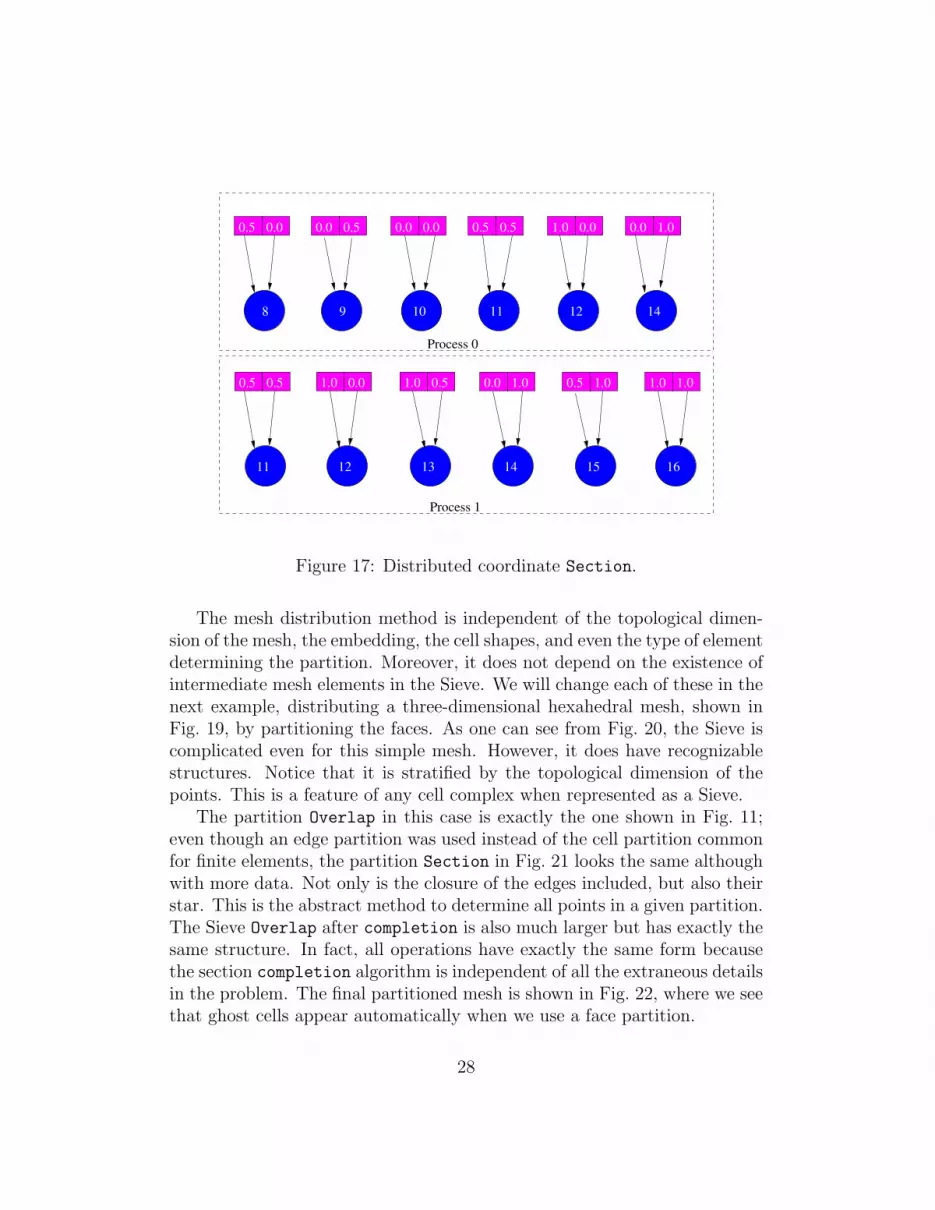
for the Mesh. In this example, we have only a coordinate Section, shownin Fig. 16. Notice that while only vertices have coordinate values, the SieveOverlap contains the triangular faces as well. Our algorithm is insensitive tothis, as the faces merely have empty cones in this Section. We now makeuse of another adapter, the Atlas, which substitutes the number of values forthe values returned by a restrict, which we use as the sizer for completion.After distribution of this Section, we have the result in Fig. 17. We are thusable to fully construct the distributed mesh in Fig. 18.

22

Figure 7: Redistributed triangular mesh.23

8

9

10

11

12

13

14 15 16

0

1

5

7

4

6

2

3

Figure 8: A simple triangular mesh.

0 1 2 3 74 65

12 1614 151311108 9

Figure 9: Sieve for mesh in Fig. 8.

24

0 1 2 4

10 8 9 8911 8 1112 9 11 14

Process 0

Figure 10: Initial local sieve on process 0 for mesh in Fig. 8.

1

1 1

0

1 1

Process 1Process 0

Figure 11: Partition point Overlap, with dark partition points, light processranks, and arrow labels representing remote points.

25

3 5 6 7 11 12 13 14 15 16

1

Figure 12: Partition section, with circular partition points and rectangularSieve point data.

0

1

3 5 6 7 11 12 13 14 15 16

3 5 6 7 11 12 13 14 15 16

35

6 7 11 12 1314 15 16

3 5 6 7 11 12 13 1415 16

Process0

Process 1

Figure 13: Sieve overlap, with Sieve points in blue, process ranks in green,and arrow labels representing remote sieve points.

26

11 13 15 15 14 1113 11 12 16 15 13

3 765

Figure 14: Cone Section, with circular Sieve points and rectangular cone

point data.

0 1 2 4

10 8 9 8911 8 1112 9 11 14

3 5 6 7

13 11 12 151311 15 1114 16 15 13

Process 0

Process 1

Figure 15: Distributed Sieve for mesh in Fig. 18.

8 11109 12 13 14 15 16

0.5 0.0 0.0 0.5 0.5 1.0 1.0 1.00.0 0.0 0.5 0.5 1.0 0.0 1.0 0.5 0.0 1.0

Figure 16: Coordinate Section, with circular Sieve points and rectangularcoordinate data.

27

11 12 13 15 1614

8 11109 12 14

0.5 0.0 0.0 0.5 0.0 0.0 0.5 0.5 1.0 0.0 0.0 1.0

0.5 0.5 1.0 0.0 1.0 0.5 0.5 1.0 1.0 1.00.0 1.0

Process 0

Process 1

Figure 17: Distributed coordinate Section.

The mesh distribution method is independent of the topological dimen-sion of the mesh, the embedding, the cell shapes, and even the type of elementdetermining the partition. Moreover, it does not depend on the existence ofintermediate mesh elements in the Sieve. We will change each of these in thenext example, distributing a three-dimensional hexahedral mesh, shown inFig. 19, by partitioning the faces. As one can see from Fig. 20, the Sieve iscomplicated even for this simple mesh. However, it does have recognizablestructures. Notice that it is stratified by the topological dimension of thepoints. This is a feature of any cell complex when represented as a Sieve.

The partition Overlap in this case is exactly the one shown in Fig. 11;even though an edge partition was used instead of the cell partition commonfor finite elements, the partition Section in Fig. 21 looks the same althoughwith more data. Not only is the closure of the edges included, but also theirstar. This is the abstract method to determine all points in a given partition.The Sieve Overlap after completion is also much larger but has exactly thesame structure. In fact, all operations have exactly the same form becausethe section completion algorithm is independent of all the extraneous detailsin the problem. The final partitioned mesh is shown in Fig. 22, where we seethat ghost cells appear automatically when we use a face partition.

28

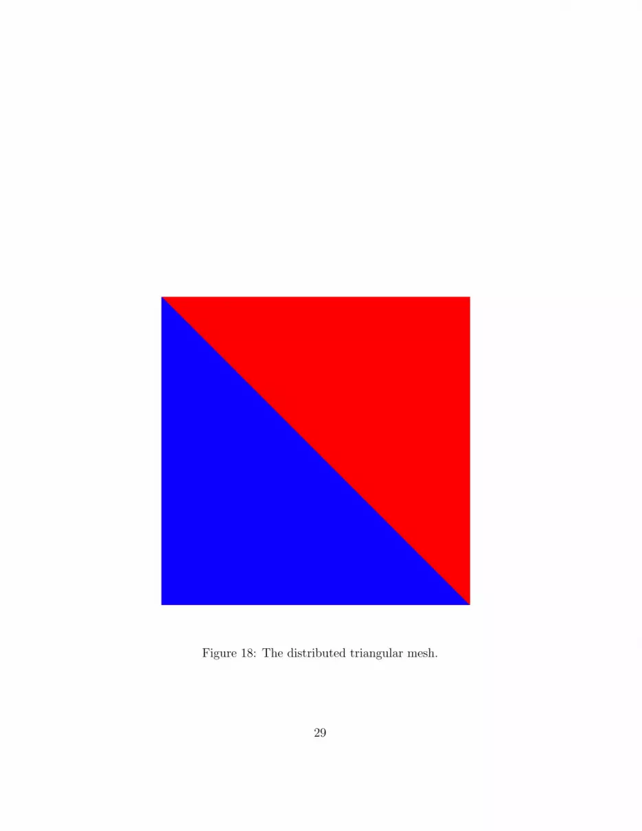
Figure 18: The distributed triangular mesh.

29

1098

11

20

29

19

28

12

21

30

13

22

31

14

23

32

15

24

33

16

25

34

18

27

17

26

0 1

23

45

67

Figure 19: A simple hexahedral mesh.

30

92

95

97

99

100

104

106

108

109

113

115

117

118

121

123

124

73

75

77

78

81

84

86

87

44

47

49

51

52

56

60

62

64

65

69

39

12

16

14

15

13

11

10

89

17

18

19

20

21

23

24

25

26

27

28

29

30

31

32

33

34

22

90

91

93

94

96

98

101

102

103

105

107

110

112

111

114

116

119

120

122

70

71

72

74

76

79

80

82

83

85

88

89

61

63

66

67

68

35

36

37

38

40

41

42

43

45

46

48

50

59

58

57

55

54

53

01

23

74

65

Figure 20: Sieve corresponding to the mesh in Fig. 19.

31

0 1 2 3 5 6 8 9 10 11 12 13 15

16 17 18 19 20 21 22 24 25 27 28 29 34

35 36 37 38 39 40 41 42 43 45 46 47 48

49 50 51 52 53 54 55 56 57 58 59 60 61

62 63 64 65 66 67 68 69 70 71 72 73 74

109

75 76 77 78 89 96 101 102 103 104 105 107 108

1

Figure 21: Partition Section, with circular partition points and rectangularSieve point data.

5 Conclusions

We have presented mesh partitioning and distribution in the context of theSieve framework in order to illustrate the power and flexibility of this ap-proach. Since we draw no distinction between mesh elements of any shape,dimension, or geometry, we may accept a partition of any element type, suchas cells or faces. Once provided with this partition and an overlap sieve,which just indicates the flow of information and is constructed automati-cally, the entire mesh can be distributed across processes by using a singleoperation, section completion. Thus, only a single parallel operation needbe portable, verifiable, or optimized for a given architecture. Moreover, thissame operation can be used to distribute data associated with the mesh, inany arbitrary configuration, according to the same partition. Thus, the highlevel of mathematical abstraction in the Sieve interface results in concretebenefits in terms of code reuse, simplicity, and extensibility.

Acknowledgements

The authors benefited from many useful discussions with Gary Miller andRob Kirby. This work was supported by the Mathematical, Information,and Computational Sciences Division subprogram of the Office of AdvancedScientific Computing Research, Office of Science, U.S. Department of Energy,

32

1098

11

20

29

19

28

12

21

13

22

15

24

16

25

34

18

27

17

0 1

23

5

6

20

29

19

28

21

30

13

22

31

14

23

32

15

24

33

16

25

34

18

27

17

26

0

3

45

67

Process 0

Process 1

Figure 22: Distributed hexahedral mesh.33

under Contract DE-AC02-06CH11357.

References

[1] Pavel S. Aleksandrov. Combinatorial Topology, volume 3. Dover, 1998.

[2] Satish Balay, Kris Buschelman, Victor Eijkhout, William D. Gropp,Dinesh Kaushik, Matthew G. Knepley, Lois Curfman McInnes, Barry F.Smith, and Hong Zhang. PETSc users manual. Technical Report ANL-95/11 - Revision 3.0.0, Argonne National Laboratory, 2009.

[3] Mark W. Beall, Joe Walsh, and Mark S. Shephard. A comparison oftechniques for geometry access related to mesh generation. EngineeringWith Computers, 20(3):210–221, 2004.

[4] Guntram Berti. Generic Software Components for Scientific Comput-ing. PhD thesis, TU Cottbus, 2000. http://www.math.tu-cottbus.

de/∼berti/diss.

[5] Glen E. Bredon. Sheaf Theory. Graduate Texts in Mathematics.Springer, 1997.

[6] Graham F. Carey, Michael L. Anderson, Brian R. Carnes, and Ben-jamin S. Kirk. Some aspects of adaptive grid technology related toboundary and interior layers. Journal of Computational Applied Math-ematics, 166(1):55–86, 2004.

[7] Karen D. Devine, Erik G. Boman, Robert T. Heaphy, Umit V.Catalyurek, and Robert H. Bisseling. Parallel hypergraph partitioningfor irregular problems. SIAM Parallel Processing for Scientific Comput-ing, February 2006.

[8] Ray Meyers et. al. SNL implementation of the TSTT mesh interface. In8th International conference on numerical grid generation in computa-tional field simulations, June 2002.

[9] Erich Gamma, Richard Helm, Ralph Johnson, and John Vlissides. De-sign Patterns. Addison-Wesley Professional, January 1995.

[10] Allen Hatcher. Algebraic Topology. Cambridge University Press, 2002.

34

[11] Bruce Hendrickson and Robert Leland. A multilevel algorithm forpartitioning graphs. In Supercomputing ’95: Proceedings of the 1995ACM/IEEE Conference on Supercomputing (CDROM), page 28, NewYork, 1995. ACM Press.

[12] George Karypis and Vipin Kumar. A parallel algorithm for multilevelgraph partitioning and sparse matrix ordering. Journal of Parallel andDistributed Computing, 48:71–85, 1998.

[13] George Karypis et al. ParMETIS Web page, 2005. http://www.cs.

umn.edu/∼karypis/metis/parmetis.

[14] Matthew G. Knepley and Dmitry A. Karpeev. Sieve implementation.Technical Report ANL/MCS to appear, Argonne National Laboratory,January 2008.

[15] Richard C. Martineau and Ray A. Berry. The pressure-corrected icefinite element method for compressible flows on unstructured meshes.Journal of Computational Physics, 198(2):659–685, 2004.

[16] E. S. Seol and Mark S. Shephard. A flexible distributed mesh datastructure to support parallel adaptive analysis. In Proceedings of the8th US National Congress on Computational Mechanics, 2005.

[17] Jonathan R. Shewchuk. Triangle: Engineering a 2D quality mesh gener-ator and Delaunay triangulator. In Ming C. Lin and Dinesh Manocha,editors, Applied Computational Geometry: Towards Geometric Engi-neering, volume 1148 of Lecture Notes in Computer Science, pages 203–222. Springer-Verlag, May 1996. From the First ACM Workshop onApplied Computational Geometry.

[18] Norman Steenrod. The Topology of Fibre Bundles. (PMS-14). PrincetonUniversity Press, April 1999.

[19] Timothy J. Tautges. MOAB-SD: Integrated structured and unstruc-tured mesh representation. Engineering With Computers, 20:286–293,2004.

[20] Timothy J. Tautges, Ray Meyers, Karl Merkley, Clint Stimpson, andCorey Ernst. MOAB: A mesh-oriented database. Technical ReportSAND2004-1592, Sandia National Laboratories, April 2004.

35

[21] Charles A. Williams, Brad Aagaard, and Matthew G. Knepley. Devel-opment of software for studying earthquakes across multiple spatial andtemporal scales by coupling quasi-static and dynamic simulations. InEos Transactions of the AGU. American Geophysical Union, 2005. FallMeeting Supplemental, Abstract S53A-1072.

36