time discretization of fbsde with polynomial growth drivers
TRANSCRIPT
The Annals of Applied Probability2015, Vol. 25, No. 5, 2563–2625DOI: 10.1214/14-AAP1056© Institute of Mathematical Statistics, 2015
TIME DISCRETIZATION OF FBSDE WITH POLYNOMIALGROWTH DRIVERS AND REACTION–DIFFUSION PDES1
BY ARNAUD LIONNET2, GONÇALO DOS REIS3 AND LUKASZ SZPRUCH
University of Oxford, University of Edinburgh and CMA/FCT/UNL,and University of Edinburgh
In this paper, we undertake the error analysis of the time discretization ofsystems of Forward–Backward Stochastic Differential Equations (FBSDEs)with drivers having polynomial growth and that are also monotone in the statevariable.
We show with a counter-example that the natural explicit Euler schememay diverge, unlike in the canonical Lipschitz driver case. This is due to thelack of a certain stability property of the Euler scheme which is essential toobtain convergence. However, a thorough analysis of the family of θ -schemesreveals that this required stability property can be recovered if the scheme issufficiently implicit. As a by-product of our analysis, we shed some light onhigher order approximation schemes for FBSDEs under non-Lipschitz condi-tion. We then return to fully explicit schemes and show that an appropriatelytamed version of the explicit Euler scheme enjoys the required stability prop-erty and as a consequence converges.
In order to establish convergence of the several discretizations, we extendthe canonical path- and first-order variational regularity results to FBSDEswith polynomial growth drivers which are also monotone. These results areof independent interest for the theory of FBSDEs.
1. Introduction. There is currently a long literature on the numerical approx-imation of FBSDE with Lipschitz conditions [Bouchard and Touzi (2004), Crisanand Manolarakis (2012), Gobet and Turkedjiev (2011), Chassagneux (2012, 2013)and references within]. In this article, we address the case of FBSDEs with drivershaving polynomial growth in the state variable, which has not been studied be-fore, and provide customized analysis of various implicit and explicit schemes.
Received September 2013; revised June 2014.1Supported by the Engineering and Physical Sciences Research Council (UK) which has funded
this work as part of the Numerical Algorithms and Intelligent Software Centre (NAIS) under GrantEP/G036136/1.
2Supported in part by the Engineering and Physical Sciences Research Council (UK) via the GrantEP/P505216/1, as well as by the Oxford-Man Institute.
3Supported by the Fundação para a Ciência e a Tecnologia (Portuguese Foundation for Scienceand Technology) through the project PEst-OE/MAT/UI0297/2014 (Centro de Matemática e Apli-cações CMA/FCT/UNL).
MSC2010 subject classifications. Primary 65C30, 60H35; secondary 60H07, 60H30.Key words and phrases. FBSDE, monotone driver, polynomial growth, time discretization, path
regularity, calculus of variations, numerical schemes.
2563
2564 A. LIONNET, G. DOS REIS AND L. SZPRUCH
The importance of FBSDEs with nonlinear drivers is due to the fruitful connec-tion between FBSDEs and partial differential equations (PDEs). Many biologi-cal and physical phenomena are modeled using PDEs of parabolic type, say for(t, x) ∈ [0, T ] ×R
d
−∂tv(t, x) −Lv(t, x) − f(t, x, v(t, x), (∇vσ)(t, x)
)= 0, v(0, x) = g(x),
with L a second-order elliptic differential operator and certain measurable func-tions f and g. A very large class of such equations can be linked to the solu-tion process �t,x = (Xt,x, Y t,x,Zt,x) of certain forward–backward stochastic dif-ferential equations (FBSDEs) with the following type of dynamics for (t, x) ∈[0, T ] ×R
d , s ∈ [t, T ] and W a Brownian-motion
Xt,xs = x +
∫ s
tb(r,Xt,x
r
)dr +
∫ s
tσ(r,Xt,x
r
)dWr,(1.1)
Y t,xs = g
(X
t,xT
)+ ∫ T
sf(r,�t,x
r
)dr −
∫ T
sZt,x
r dWr,(1.2)
via the so-called nonlinear Feynman–Kac formula: v(T − t, x) = Yt,xt [see, e.g.,
El Karoui, Peng and Quenez (1997)].In many applications of interest, like reaction–diffusion type equations, the
function f is a polynomial (in v), for example, the Allen–Cahn equation, theFitzHugh–Nagumo equations (with or without recovery) or the standard nonlin-ear heat and Schrödinger equation [see Henry (1981), Rothe (1984), Estep, Larsonand Williams (2000), Kovács (2011) and references].
Motivated by these applications, we look further at the connection betweenparabolic PDEs and FBSDEs with monotone drivers f of polynomial growth [seePardoux (1999), Briand and Carmona (2000) and Briand et al. (2003)]. By mono-tonicity, we mean that 〈v′ − v,f (v′) − f (v)〉 ≤ μ|v′ − v|2, for some μ ≥ 0, andany v, v′ (one can also find the terminology that f is one-sided Lipschitz). We ex-tend the above mentioned works by providing further regularity estimates for theFBSDE in question (modulus of continuity, path and variational regularity). Thenwe proceed to a thorough analysis of various numerical methods that open the doorto Monte Carlo methods for solving numerically the corresponding PDEs.
The work and results we present should be understood as a first step in the nu-merical analysis of FBSDE with monotone drivers of polynomial growth, widerthan the Lipschitz driver BSDE setting, with the intent of deepening the appli-cability of FBSDEs to reaction–diffusion equations. Moreover, we work withoutassuming knowledge on the density function or the moment generating functionof the forward process X. In some applications where X is simply the Brown-ian motion, it is possible to derive a numerical solver that takes advantage on thisknowledge; see, for example, Zhang, Gunzburger and Zhao (2013). The work wedevelop aims at black-box type algorithms which do not take advantage of any ofthe specific forms the FBSDEs coefficients may take.
NUMERICS FOR FBSDE WITH POLYNOMIAL GROWTH DRIVERS 2565
A motivating example. To better understand why the explicit Euler schemeseems not to be suitable for approximating the solution to BSDEs with non-Lipschitz drivers, let us consider the following simple example (for further detailsand notational setup, see Section 2 and Appendix A.1):
Yt = ξ −∫ 1
tY 3
s ds −∫ 1
tZs dWs, t ∈ [0,1](1.3)
with the terminal condition ξ ∈ F1. For any ξ ∈ Lp for p ≥ 2, there exists4 aunique (square-integrable) solution (Y,Z) to the above BSDE.
Fix the number of time-discretization points to be N + 1 > 0. The explicit Eu-ler scheme for the above equation with uniform time step h = 1/N is, with thenotation Yi := Yi/N , given by
Yi = E[Yi+1 − Y 3
i+1h|Fi
]= E[Yi+1
(1 − hY 2
i+1)|Fi
],
(1.4)i = 0, . . . ,N − 1,
where YN = ξ .It is a simple calculation (see Appendix A.1 for the details) to show that if
ξ ≥ 2√
N then |Yi | ≥ 22N−i√N for i = 0, . . . ,N.(1.5)
With this simple computation in mind, it is possible to show that there exists arandom variable ξ whose moments of any order are finite and for which the explicitEuler scheme diverges. The result below is a corollary of Lemma A.2 that can befound in Appendix A.1.
LEMMA 1.1. Let πN be the uniform grid over the interval [0,1] with N + 1points, N an even number (t = 1/2 is common to all grids πN ). For any ξ ∈Lp(F1), for p ≥ 2, let (Y,Z) denote the solution to (1.3).
Then there exists a random variable ξ ∈ Lp \ L∞ for any p ≥ 2 such that
limN→∞E
[∣∣Y (N)1/2
∣∣]= +∞,
where Y(N)1/2 is the Euler approximation of Y on the time point t = 1/2 via (1.4)
over the grids πN .
The special random variable ξ we work with is normally distributed and it isknown that P[|ξ | > 2
√N ] is exponentially small (see Lemma A.1). What our
counter-example shows is that although ξ may take very large values on an eventwith exponentially small probability, the impact of these very large values whenpropagated through the Euler explicit scheme is doubly-exponential [see (1.5)].
4Existence and uniqueness follows from Section 2 in Pardoux (1999) or Theorem 2.2 below.
2566 A. LIONNET, G. DOS REIS AND L. SZPRUCH
This double-exponential impact is precisely a consequence of the superlinearityof the driver. In general, the terminal condition ξ is an unbounded random variable(RV) so there is a positive probability of the scenario where ξ ≥ 2
√N no matter
how small a time-step we choose. This indicates that, in general, the explicit Eu-ler scheme may diverge, as it happens in SDE context Hutzenthaler, Jentzen andKloeden (2011). Therefore, one needs to seek alternative (e.g., implicit) approx-imations for BSDE with polynomial drivers that are also monotone and/or findconditions under which it is possible for the explicit scheme to work, as explicitschemes have certain computational advantages over implicit ones.
Our contribution.
• We extend the canonical Zhang path regularity theorem [see Ma and Zhang(2002), Imkeller and dos Reis (2010a)], originally proved under Lipschitz as-sumptions, to our polynomial growth monotone driver setting proving in be-tween all the required stochastic smoothness results; essentially all first-ordervariations of the solution processes and estimates on the modulus of continu-ity.
• For our non-Lipschitz setting, we provide a thorough analysis of the familyof θ -schemes, where θ ∈ [0,1] characterizes the degree of implicitness of thescheme. Contrary to the FBSDEs with Lipschitz driver we show that choos-ing θ ≥ 1/2 is essential to ensure the stability of the scheme, in a similar wayto the SDE context [see Mao and Szpruch (2013)]. This is to our knowledgethe first result in the numerical BSDEs literature that shows a superior sta-bility of the implicit scheme over the standard explicit one. We also general-ize the concept of stability for discretization schemes [see that in Chassagneux(2012, 2013)]. This, among others things, paves a way for deriving higher orderapproximations schemes for FBSDEs with non-Lipschitz drivers. As an exam-ple, we prove a higher order of convergence for the trapezoidal scheme (the caseθ = 1/2).
• We construct an appropriately tamed version of the explicit Euler scheme forwhich the required stability property can be recovered. This allows us to obtainconvergence of the scheme. Interestingly enough, in the special case where thedriver of the FBSDEs does not depend on the SDE solution it is enough to appro-priately tame the terminal condition, leaving the rest of the Euler approximationunchanged.
As a rule of thumb, implicit schemes tend to be more robust than explicit ones.Unfortunately implicit schemes involve solving an implicit equation, which createsan extra layer of complexity when compared to explicit schemes. A secondary aimof this work is to distinguish under which conditions explicit and implicit schemescan be used.
As standard in numerical analysis, we derive the global error estimates of var-ious numerical schemes by analyzing their one-step errors and stability proper-ties (which allows us to study how errors propagate with time). We formulate the
NUMERICS FOR FBSDE WITH POLYNOMIAL GROWTH DRIVERS 2567
Fundamental Lemma [following the nomenclature from Milstein and Tretyakov(2004)] that states how to estimate the global error of a stable approximationscheme in terms of its local errors. The lemma is proved under minimal assump-tions. We stress that a similar approach has been used in Chassagneux and Crisan(2012) and Chassagneux (2012, 2013); however, their results are not sufficientlygeneral to deal with non-Lipschitz drivers.
The structure of the global error estimate given by the Fundamental Lemma al-lows us to study in a very easy and transparent way the special case of the θ -schemewith θ = 1/2 (trapezoidal rule) which has a higher order of convergence. In thiscontext, we also conjecture a candidate for the second-order scheme.
Concerning the implementation of the presented schemes, we propose an alter-native estimator of the component Z whose standard deviation, contrary to usualestimator, does not explode as the time step vanishes.
Finally, we note that in proving convergence for the mostly-implicit schemes,we prove Lp-type uniform bounds for the scheme, thus extending the classi-cal L2-bound obtained previously for the discretization of Lipschitz FBSDEs[see Bouchard and Touzi (2004), Gobet and Turkedjiev (2011) and referencestherein].
This work is organized as follows. In Section 2, we define notation and recallstandard results from the literature. In Section 3, we establish first-order varia-tional results for the solution of the FBSDEs as well as stating the path regularityresults required for the study of numerical schemes within the FBSDE framework.The remaining sections contain the discussion of several numerical schemes: inSection 4, we define the numerical discretization procedure and state general es-timates for integrability and on the local errors. In Section 5, we establish theconvergence of the implicit dominating schemes and in Section 6 the convergenceof the tamed explicit scheme [after the terminology of Hutzenthaler, Jentzen andKloeden (2012)]. In Section 7, we give some numerical examples.
2. Preliminaries.
2.1. Notation. Throughout let us fix T > 0. We work on a canonical Wienerspace (�,F,P) carrying a d-dimensional Wiener process W = (W 1, . . . ,Wd) re-stricted to the time interval [0, T ]. We denote by F = (Ft )t∈[0,T ] its natural filtra-tion enlarged in the usual way by the P-zero sets and by E and E[·|Ft ] = Et [·] theusual expectation and conditional expectation operator, respectively.
For vectors x = (x1, . . . , xd) in the Euclidean space Rd , we denote by | · | and
〈·, ·〉 the canonical Euclidean norm and inner product (resp.) while ‖ · ‖ is thematrix norm in R
k×d (when no ambiguity arises we use | · | as ‖ · ‖); for A ∈ Rk×d
A∗ denotes the transpose of A; Id denotes the d-dimensional identity matrix. Fora map b :Rm → R
d , we denote by ∇b its Rd×m-valued Jacobi matrix (gradient
in case d = 1) whenever it exists. To denote the j th first derivative of b(x) for
2568 A. LIONNET, G. DOS REIS AND L. SZPRUCH
x ∈ Rm, we write ∇xj
b (valued in Rd×1). For b(x, y) :Rm × R
d → Rk , we write
∇xh or ∇yh to refer to its Jacobi matrix (gradient if k = 1) with relation to x and y,respectively. denotes the canonical Laplace operator.
We define the following spaces for p > 1, q ≥ 1, n,m,d, k ∈ N: C0,n([0, T ] ×R
d,Rk) is the space of continuous functions endowed with the ‖ · ‖∞-norm thatare n-times continuously differentiable in the spatial variable; C
0,nb contains all
bounded functions of C0,n; the first superscript 0 is dropped for functions indepen-dent of time; Lp(Ft ,R
d), t ∈ [0, T ], is the space of d-dimensional Ft -measurableRVs X with norm ‖X‖Lp = E[|X|p]1/p < ∞; L∞ refers to the subset of es-sentially bounded RVs; Sp([0, T ] × R
d) is the space of d-dimensional mea-surable F -adapted processes Y satisfying ‖Y‖Sp = E[supt∈[0,T ] |Yt |p]1/p < ∞;S∞ refers to the subset of Sp(Rd) of absolutely uniformly bounded processes;Hp([0, T ]×R
n×d) is the space of d-dimensional measurable F -adapted processesZ satisfying ‖Z‖Hp = E[(∫ T
0 |Zs |2 ds)p/2]1/p < ∞; Dk,p(Rd) and Lk,d(Rd) arethe spaces of Malliavin differentiable RVs and processes; see Appendix A.2.
2.2. Setting. We want to study the forward–backward SDE system with dy-namics (1.1)–(1.2), for (t, x) ∈ [0, T ] × R
d and �t,x := (Xt,x, Y t,x,Zt,x). Herewe work, for s ∈ [t, T ], with the filtration F t
s := σ(Wr − Wt : r ∈ [t, s]), com-pleted with the P-null measure sets of F . Concerning the functions appearing in(1.1) and (1.2) we will work with the following assumptions.
(HX0). b : [0, T ] ×Rd → R
d , σ : [0, T ] ×Rd → R
d×d are 1/2-Hölder con-tinuous in their time variable, are Lipschitz continuous in their spatial variables,satisfy ‖b(·,0)‖∞ + ‖σ(·,0)‖∞ < ∞, and hence satisfy |b(·, x)| + |σ(·, x)| ≤K(1 + |x|) for some K > 0.
(HY0). g :Rd → Rk is a Lipschitz function of linear growth; f : [0, T ] ×
Rd × R
k × Rk×d → R
k is a continuous function and for some L,Lx,Ly,Lz > 0for all t, t ′, x, x′, y, y′, z, z′ it holds that
∃m ≥ 1∣∣f (t, x, y, z)
∣∣≤ L + Lx |x| + Ly |y|m + Lz‖z‖,⟨y′ − y,f
(t, x, y′, z
)− f (t, x, y, z)⟩≤ Ly
∣∣y′ − y∣∣2,
(2.1) ∣∣f (t, x, y, z) − f(t ′, x′, y, z′)∣∣≤ Lt
∣∣t − t ′∣∣1/2
+ Lx
∣∣x − x′∣∣+ Lz
∥∥z − z′∥∥.(HY0loc). (HY0) holds and, given Ly , it holds for all t, x, y, y′, z that∣∣f (t, x, y, z) − f
(t, x, y′, z
)∣∣≤ Ly
(1 + |y|m−1 + ∣∣y′∣∣m−1)∣∣y − y′∣∣.(2.2)
(HXY1). (HX0), (HY0loc) hold; g ∈ C1 and b,σ,f ∈ C0,1.
We state next a useful consequence of the monotonicity condition (2.1).
NUMERICS FOR FBSDE WITH POLYNOMIAL GROWTH DRIVERS 2569
REMARK 2.1. Under assumption (HY0), for all t, x, y, y′, z, z′ and any α > 0,we have ⟨
y′ − y,f(t, x, y′, z′)− f (t, x, y, z)
⟩= ⟨
y′ − y,f(t, x, y′, z′)± f
(t, x, y, z′)− f (t, x, y, z)
⟩≤ Ly
∣∣y′ − y∣∣2 + Lz
∣∣y′ − y∣∣∣∣z′ − z
∣∣≤ (Ly + α)
∣∣y′ − y∣∣2 + L2
z
4α
∣∣z′ − z∣∣2.
Moreover, ⟨y,f (t, x, y, z)
⟩= ⟨
y − 0, f (t, x, y, z) − f (t, x,0, z)⟩+ ⟨
y,f (t, x,0, z)⟩
(2.3)≤ Ly |y|2 + |y|(L + Lx |x| + Lz|z|)≤ (Ly + α)|y|2 + 3L2
4α+ 3L2
x
4α|x|2 + 3L2
z
4α|z|2.
2.3. Basic results. In this subsection, we recall several auxiliary results con-cerning the solution of (1.1)–(1.2) that will become useful later. These results fol-lows from Pardoux (1999) and Briand and Carmona (2000).
THEOREM 2.2 (Existence and uniqueness). Let (HX0) and (HY0) hold. ThenFBSDE (1.1)–(1.2) has a unique solution (X,Y,Z) ∈ Sp ×Sp ×Hp for any p ≥ 2.Moreover, it holds for some constant Cp > 0 that
‖Y‖pSp + ‖Z‖p
Hp ≤ Cp
{∥∥g(XT )∥∥pLp + ∥∥f (·,X·,0,0)
∥∥pHp
}(2.4)
≤ Cp
(1 + |x|p).
PROOF. The existence and uniqueness results for SDE (1.1) follow from stan-dard SDE literature. The existence and uniqueness result for the BSDE followsfrom Proposition 2.2 in Pardoux (1999), since the SDE results imply that X ∈ Sp
for any p ≥ 2, along with linear growth in x of g and f . The estimates for Y ∈ Sp
for any p ≥ 2 and Z ∈Hp follow from the pathwise inequality
|Yt |2 +(
1 − 3L2z
2α
)Et
[∫ T
t|Zu|2 du
](2.5)
≤ Cα,T ,tEt
[∣∣g(XT )∣∣2 +
∫ T
t
3
4α
∣∣f (u,Xu,0,0)∣∣2 du
],
where Cα,T ,t = exp{2(Ly + α)(T − t)}, for any α > 0 and t ∈ [0, T ]. This lastinequality follows from the proof of Proposition 2.2 and Exercise 2.3 in Pardoux(1999) [see also Theorem 3.6 in Briand and Carmona (2000)]. �
2570 A. LIONNET, G. DOS REIS AND L. SZPRUCH
We now state a result concerning a priori estimates for BSDEs.
THEOREM 2.3 (A priori estimate). Let p ≥ 2 and for i ∈ {1,2}, let �i =(Xi, Y i,Zi) be the solution of FBSDE (1.1)–(1.2) with functions bi, σ i, gi, f i sat-isfying (HX0)–(HY0). Then there exists Cp > 0 depending only on p and the con-stants in the assumptions such that for i ∈ {1,2}∥∥Y 1 − Y 2∥∥p
Sp + ∥∥Z1 − Z2∥∥pHp
≤ Cp
{E
[∣∣g1(X1T
)− g2(X2T
)∣∣p(2.6)
+(∫ T
0
∣∣f 1(s,X1s , Y
is ,Z
is
)− f 2(s,X2s , Y
is ,Z
is
)∣∣ds
)p]}.
PROOF. See Proposition 3.2 and Corollary 3.3 in Briand and Carmona (2000).�
COROLLARY 2.4 (Markov property and sample path continuity). Let (HX0)and (HY0) hold. The mapping (t, x) �→ Y
t,xt (ω) is continuous. There exist two
B([0, T ]) ⊗ B(Rk) and B([0, T ]) ⊗ B(Rk×d) measurable deterministic functionsu and v (resp.) s.t.
Y t,xs = u
(s,Xt,x
s
), s ∈ [t, T ],dP-a.s.,
(2.7)Zt,x
s = v(s,Xt,x
s
)σ(s,Xt,x
s
), s ∈ [t, T ],dP× ds-a.s.
Moreover, the Markov property holds Yt,xt+h = Y
t+h,Xt,xt+h
t+h for any h ≥ 0 and u ∈C0,0([0, T ] ×R
k).
PROOF. See Section 3 in Pardoux (1999). The sample path continuityof Y
t,xt follows from the mean-square continuity of (Y t,x
s )s∈[t,T ] for x ∈ Rk ,
0 ≤ t ≤ s ≤ T , which in turn follows from inequality (2.6), combined with theLipschitz property of x �→ g(x) and (t, x) �→ f (t, x, ·, ·) along with the continuityproperties of (t, x) �→ Xt,x· solution to (1.1).
The Markov property follows from Remark 3.1 Pardoux (1999) and the conti-nuity of u(t, x) is implied by that of Y
t,xt . �
2.4. Nonlinear Feynman–Kac formula. As pointed out in the Introduction, ouraim is to deepen the connection between FBSDEs and PDEs via the so-called non-linear Feynman–Kac formula, that is, we study the probabilistic representation ofthe solution to a class of parabolic PDEs on R
k with polynomial growth coeffi-cients that are associated with FBSDE (1.1)–(1.2). For (t, x) ∈ [0, T ]×R
d , denoteby L the infinitesimal generator of the Markov process Xt,x solution to (1.1)
L := 1
2
d∑i,j=1
([σσ ∗]
ij
)(t, x)∂2
xixj+
d∑i=1
bi(t, x)∂xi,(2.8)
NUMERICS FOR FBSDE WITH POLYNOMIAL GROWTH DRIVERS 2571
and consider for a function v = (v1, . . . , vk) the following system of backwardsemi-linear parabolic PDEs for i ∈ {1, . . . , k}: v(T , x) = g(x) and
−∂tvi(t, x) −Lvi(t, x) − fi
(t, x, v(t, x), (∇vσ)(t, x)
)= 0.(2.9)
In rough, it can be easily proved using Itô’s formula that if v ∈ C1,2([0, T ] ×R
d;Rk) solves the above PDE then Yt := v(t,Xt ) and Zt := (∇vσ)(t,Xt) solvesBSDE (1.2) [see Proposition 3.1 in Pardoux (1999)]. But the more interesting re-sult is the converse one, that is, that u(t, x) := Y
t,xt is the solution of the PDE (in
some sense). It was established in Theorem 3.2 of Pardoux (1999) (recalled next)that indeed (t, x) �→ Y
t,xt is the viscosity solution of the PDE.
THEOREM 2.5. Let (HX0), (HY0) hold and take (t, x) ∈ [0, T ] × Rd . Fur-
thermore, assume that the ith component of the driver function f depends only onthe ith row of the matrix z ∈ R
k×d , that is, fi(t, x, y, z) = fi(t, x, y, zi).Then u(t, x) := Y
t,xt is a continuous function of (t, x) that grows at most poly-
nomially at infinity and is a viscosity solution of (2.9) [in the sense of Definition 3.2in Pardoux (1999)].
REMARK 2.6 (Multi-dimensional case). The proof of Theorem 2.5 relies ona BSDE comparison theorem that holds only in the case k = 1 (i.e., when Y isone-dimensional). Nonetheless, with the restriction imposed by (HY0), it is stillpossible to use the said comparison theorem to prove Theorem 2.5, we point thereader to Theorem 2.4 and Remark 2.5 in Pardoux (1999).
It is possible to show that (t, x) �→ Yt,xt is the solution to (2.9) not only in the
viscosity sense, but also in weak sense (in weighted Sobolev spaces), this has beendone in Matoussi and Xu (2008) and Zhang and Zhao (2012).
2.5. Examples. One equation covered by our setting is the FitzHugh–NagumoPDE with recovery, used in biology and related to the modeling of the electricaldistribution of the heart or the potential in neurons.
EXAMPLE 2.7 (The FH–N equation with recovery). Let (t, x) ∈ [0, T ] ×Rd ,
g = (gu, gv), f = (fu, fv) and g,f, (u, v) : [0, T ] × Rd → R
2. The FH–N PDEhas the dynamics: u(T , ·) = gu(·), v(T , ·) = gv(·) and
−∂tu − 12u − fu(u, v) = 0, −∂tv − v − fv(u, v) = 0,
where fu(u, v) = u − u3 + v and fv(u, v) = u − v. f clearly satisfies (HY0) and(HY0loc).
A simpler setup of the above model is its one-dimensional version.
2572 A. LIONNET, G. DOS REIS AND L. SZPRUCH
EXAMPLE 2.8 (FH–N equation without recovery). For (t, x) ∈ [0, T ]×R theFH–N equation without recovery is described by
−∂tu − 12u − (
cu3 + bu2 − au)= 0, u(T , x) = g(x).(2.10)
When c = −1, b = 1 + a, a ∈ R and with the choice of g(x) = (1 + ex)−1, onecan verify that the C∞
b solution u to (2.10) is given by
u(t, x) = (1 + exp
{x − (1/2 − a)(T − t)
})−1 ∈ C∞b
([0, T ] ×R).(2.11)
The FBSDE corresponding to this PDE is given by (1.1)–(1.2) with the followingdata:
b(·, ·) = 0; σ(·, ·) = 1; f (t, x, y, z) = cy3 + by2 − ay;c = −1; b = 1 + a,
and the terminal condition function g is given above. Both (HX0) and (HY0loc)hold (for any a, notice that u ≥ 0 for any a) and the theory we develop throughoutapplies to this class of examples. We will use the case a = −1 in our simulations.
3. Representation results, path regularity and other properties. As seenbefore u(t, x) := Y
t,xt is a viscosity solution of PDE (2.9). If u ∈ C1,2, we would
also obtain the representation of the process Z as Zt,xt = (∇xuσ)(t, x), but in view
of Theorem 2.5 we have not given meaning to ∇xu. The main aim of this sectionis to first prove some representation formulas, that express Z as a function of Y
and X, then use these representation formulas to obtain the so-called L2- (and Lp-)path regularity results needed to prove the convergence of the numerical discretiza-tion of FBSDE (1.1)–(1.2) in the later sections. A by-product of these results is theexistence of ∇xu.
3.1. Differentiability in the spatial parameter. Take the system (1.1)–(1.2) intoaccount. We now show that the smoothness of the FBSDE parameters b,σ, g, f
carries over to the solution process � = (X,Y,Z).
THEOREM 3.1. Let (HXY1) hold and (t, x) ∈ [0, T ] ×Rd .
Then u [from (2.7)] is continuously differentiable in its spatial variable. More-over, the triple ∇x�
t,x = (∇xXt,x,∇xY
t,x,∇xZt,x) ∈ Sp ×Sp ×Hp for any p ≥ 2
and solves for 0 ≤ t ≤ s ≤ T⎧⎪⎪⎪⎪⎪⎪⎪⎪⎪⎪⎪⎨⎪⎪⎪⎪⎪⎪⎪⎪⎪⎪⎪⎩
∇xXt,xs = Id +
∫ s
t(∇xb)
(r,Xt,x
r
)∇xXt,xr dr
+∫ s
t(∇xσ )
(r,Xt,x
r
)∇xXt,xr dWr,
∇xiY t,x
s = (∇xg)(X
t,xT
)∇xiX
t,xT −
∫ T
s∇xi
Zt,xr dWr
+∫ T
tF(r,∇xi
�t,xr
)dr
(3.1)
NUMERICS FOR FBSDE WITH POLYNOMIAL GROWTH DRIVERS 2573
for i ∈ {1, . . . , d} and with5
F : (ω, r, x,χ,ϒ,�)
�→ (∇xf )(r,�t,x
r
) · χ + (∇yf )(r,�t,x
r
) · ϒ + (∇zf )(r,�t,x
r
) · �.
There exists a positive constant Cp independent of x such that
sup(t,x)∈[0,T ]×Rd
∥∥(∇xYt,x,∇xZ
t,x)∥∥Sp×Hp ≤ Cp.(3.2)
Furthermore, for u as in (2.7) we have for x ∈ Rd and 0 ≤ t ≤ s ≤ T
∇xYt,xs = (∇xu)
(s,Xt,x
s
)∇xXt,xs , P-a.s. and
(3.3)‖∇xu‖∞ < ∞.
We recall that ∇xYt,x is R
k×d -valued and ∇xiY t,x denotes its ith column we
use a similar notation follows for ∇xX and ∇xZ.
PROOF OF THEOREM 3.1. Throughout fix (t, x) ∈ [0, T ] × Rd and let
{ei}i∈{1,...,d} be the canonical unit vectors of Rd . Let i ∈ {1, . . . , d}.The results concerning SDE (1.1) follow from those in Section 2.5 in Imkeller
and dos Reis (2010a). We start by showing that the partial derivatives (∇xiY t,x,
∇xiZt,x) for any i exist, then we will show the full differentiability. We start
by proving that (3.1) has indeed a solution for every i. Unfortunately, the driverof (3.1) does not satisfy (HY0), and hence we cannot quote Theorem 2.2 directly;we use a more general result from Briand et al. (2003). We remark though, that thetechniques used to obtain moment estimates of the form of (2.4) and (2.6) are thesame in both Briand et al. (2003) and Pardoux (1999).
FBSDE (3.1) has a unique solution �t,x,i := (∇xiXt,x,Ut,x,i, V t,x,i) ∈ Sp ×
Sp × Hp for any p ≥ 2, where (Ui,V i) replaces (∇xiY,∇xi
Z). This followsby a direct application of Theorem 4.2 in Briand et al. (2003). It is easyto see that under (HXY1) the conditions (H1)–(H5) in Briand et al. [(2003),pages 118–119] are satisfied. First, under (HXY1), standard SDE theory [see,e.g., Theorem 2.4 in Imkeller and dos Reis (2010a)] ensures that ∇xX ∈ Sp forall p ≥ 2, which along with ∇xg,∇xf ∈ C
0,0b , implies in turn that the termi-
nal condition (∇xg)(Xt,xT )∇xi
Xt,xT ∈ L
pFT
and the term (∇xf )(·,�t,x· )∇xiXt,x· =
F(·,∇xiXt,x· ,0,0) ∈ Sp for any p ≥ 2. Given the linearity of F and the Lipschitz
property of f in its z-variable, it follows that F is uniformly Lipschitz in �. More-
5The term (∇zf )(·,�) · � can be better understood if one interprets z in f not as in Rk×d but as
(Rd)k , that is, f receives not a matrix but its Rd -valued k lines.
2574 A. LIONNET, G. DOS REIS AND L. SZPRUCH
over, since f satisfies (2.1) it implies that F is monotone6 in ϒ , that is,⟨ϒ − ϒ ′, (∇yf )
(·,�t,x·) · (ϒ − ϒ ′)⟩≤ Ly
∣∣ϒ − ϒ ′∣∣2 ∀ϒ,ϒ ′ ∈Rk.(3.4)
The continuity of ϒ �→ F(r, x,χ,ϒ,�) is also clear. Finally, the linearity of F ,the fact that � ∈ Sp × Sp × Hp for any p ≥ 2 and (2.2) implies that condi-tion (H5) in Briand et al. (2003) is also satisfied, that is, that for any R > 0,sup|ϒ |≤R |F(r, x,∇xi
Xt,xr ,ϒ,0)−F(r, x,∇xi
Xt,xr ,0,0)| ∈ L1([t, T ]×�). We are
therefore under the conditions of Theorem 4.2 in Briand et al. (2003), as claimed.In view of (2.3) and the linearity of F one can obtain moment estimates in the
style of (2.4) by following arguments similar to those in the proof of Theorem 2.2[recall that (2.3) takes in this case a very simple form]. In view of (2.4), we have(recall that ∇X ∈ Sp for all p ≥ 2)∥∥Ui
∥∥pSp + ∥∥V i
∥∥pHp
≤ Cp
{∥∥(∇xg)(X
t,xT
)∇xiX
t,xT
∥∥pLp + ∥∥(∇xf )
(·,�t,x·)∇xi
Xt,x·∥∥pHp
}(3.5)
≤ Cp
∥∥∇xiXt,x
∥∥pSp ≤ Cp,
where Cp does not depend on x, t or i.In order to obtain results on the first-order variation of the solution, we follow
standard BSDE techniques used already in Imkeller and dos Reis (2010a), Briandand Confortola (2008) or dos Reis, Réveillac and Zhang (2011); we start by study-ing the behavior of �t,x+εei − �t,x for any ε > 0. Take h ∈ R
d . Via the stabilityof SDEs and inequality (2.6) [and (HY0)], it is clear that a constant Cp > 0 inde-pendent of x exists such that
limh→0
∥∥�t,x+h − �t,x∥∥Sp×Sp×Hp ≤ lim
h→0Cp
∥∥Xx+h − Xx∥∥Sp
(3.6)≤ lim
h→0Cp|h| = 0.
Define
δ�ε,i := (δXε,i, δY ε,i, δZε,i)
:= (�t,x+εei − �t,x)/ε − (∇xi
Xt,x,Ut,x,i, V t,x,i)for which
δY ε,is =
[1
ε
(g(X
t,x+εei
T
)− g(X
t,xT
))− (∇xg)(X
t,xT
)∇xiX
t,xT
]−∫ T
sδZε,i
r dWr
+∫ T
s
[1
ε
(f(r,�t,x+εei
r
)− f(r,�t,x
r
))(3.7)
− F(r, x,∇xi
Xt,xr ,U t,x,i
r , V t,x,ir
)]dr.
6This follows easily from the differentiability of f , its monotonicity in y and the definition ofdirectional derivative.
NUMERICS FOR FBSDE WITH POLYNOMIAL GROWTH DRIVERS 2575
Using the differentiability of the involved functions, we can re-write (3.7) as alinear FBSDE with random coefficients satisfying in its essence a (HY0) type as-sumption: for s ∈ [t, T ], j ∈ {1, . . . , d}⎧⎪⎪⎪⎪⎪⎪⎪⎪⎪⎪⎪⎪⎪⎪⎪⎨⎪⎪⎪⎪⎪⎪⎪⎪⎪⎪⎪⎪⎪⎪⎪⎩
δXε,js = 0 +
∫ s
t
[bε,jx (r)δXε,j
r + δ∇bεr∇xj
Xt,xr
]dr
+∫ s
t
[σε,j
x (r)δXε,jr + δ∇σε
r ∇xjXt,x
r
]dWr,
δY ε,is = [
gε,ix (T )δX
ε,iT + δ∇gε
T ∇xiX
t,xT
]− ∫ T
sδZε,i
r dWr
+∫ T
s
[f ε,i
x (r)δXε,ir + f ε,i
y (r)δY ε,ir + f ε,i
z (r)δZε,ir
+ δ∇f εr · (∇xi
Xt,xr ,U t,x,i
r , V t,x,ir
)]dr,
(3.8)
where δ∇f and δ∇ϕ denote the differences
δ∇f ε· := (f ε,i
x , f ε,iy , f ε,i
z
)(·) − (∇xf,∇yf,∇zf )
(·,�t,x·)
and
δ∇ϕε· := ϕε,ix (·) − ∇xϕ
(·,�t,x·),
for ϕ ∈ {b,σ, g} (with some abuse of notation) and r ∈ [t, T ], and where we de-fined
ϕε,ix (r) :=
∫ 1
0(∇xϕ)
(r, (1 − λ)Xt,x
r + λXt,x+εeir
)dλ
=∫ 1
0(∇xϕ)
(r,Xt,x
r + λ(Xt,x+εei
r − Xt,xr
))dλ,
and f ε,i∗ for ∗ ∈ {x, y, z} in the following way:
f ε,iz (r) :=
∫ 1
0(∇zf )
(r,Xt,x+εei
r , Y t,x+εeir ,Zt,x
r + λ(Zt,x+εei
r − Zt,xr
))dλ,
f ε,iy (r) :=
∫ 1
0(∇yf )
(r,Xt,x+εei
r , Y t,xr + λ
(Y t,x+εei
r − Y t,xr
),Zt,x
r
)dλ,
f ε,ix (r) :=
∫ 1
0(∇xf )
(r,Xt,x
r + λ(Xt,x+εei
r − Xt,xr
), Y t,x
r ,Zt,xr
)dλ.
The assumptions imply immediately that bε,ix , σ ε,i
x , f ε,ix , f ε,i
z are uniformlybounded, while f ε,i
y ∈ Sp , p ≥ 2 (thanks to HY0loc). Furthermore, using esti-mate (2.4) [along with ‖Xt,x‖p
Sp ≤ Cp(1 + |x|p)], (3.5), (3.6), the continuity ofϕ ∈ {b,σ, g} and its derivative it is easy to see that, in combination with the domi-nated convergence theorem, one has
limε→0
{∥∥ϕε,ix (·) − ∇xϕ
(·,�t,x·)∥∥
Sp
(3.9)+ ∥∥(f ε,i
x , f ε,iy , f ε,i
z
)(·) − (∇xf,∇yf,∇zf )
(·,�t,x·)∥∥
Hp
}= 0.
2576 A. LIONNET, G. DOS REIS AND L. SZPRUCH
We remark that in the above limit a localization argument for the convergenceof f ε,i
y (·) to ∇yf (·,�·) is required, namely that we work inside a ball (of anygiven radius) centered around x in which all points x + εei ∈ R
d as ε vanishes arecontained. We do not detail the argumentation since it is similar to that given in,for example, Imkeller and dos Reis (2010a), Briand and Confortola (2008) or dosReis, Réveillac and Zhang (2011).
With this in mind we return to (3.7), written in the form of (3.8), and since itis a linear FBSDE satisfying the monotonicity condition (2.1) we have via Corol-lary 3.3 in Briand and Carmona (2000) [essentially our moment estimate (2.4) forFBSDE (3.8)] in combination with (3.5), (3.6) and (3.9), that for any i
limε→0
∥∥∥∥1
ε
(�t,x+εei − �t,x)− (∇xi
Xt,x,Ut,x,i, V t,x,i)∥∥∥∥Sp×Sp×Hp
= 0 ∀p ≥ 2.
Since the limit exists we identify (∇xiY t,x,∇xi
Zt,x) with (Ut,x,i , V t,x,i) and,moreover, estimate (3.5) implies estimate (3.2). Furthermore, the above limit im-plies in particular that (take s = t)
∇xiu(t, x) = lim
ε→0
1
ε
[u(t, x + εei) − u(t, x)
]= lim
ε→0
1
ε
[Y
t,x+εeit − Y
t,xt
]= ∇xiY
t,xt .
Observing that the RHS of (3.5) is a constant independent of t ∈ [0, T ], x ∈ Rd
and i ∈ {1, . . . , d} we can conclude that
‖∇xiu‖∞ = sup
(t,x)∈[0,T ]×Rd
∣∣∇xiY
t,xt
∣∣< ∞.(3.10)
It is clear that (∇xiY t,x
s )s∈[t,T ] is continuous in its time parameter as it is a solu-tion to a BSDE; we now focus on the continuity of x �→ ∇xi
Yt,xt . Let x, x′ ∈ R
d .The difference ∇xi
Y t,x − ∇xiY t,x′
is the solution to a linear FBSDE followingfrom (3.1). As before, it is easy to adapt the computations and apply Corollary 3.3in Briand and Carmona (2000) [essentially our moment estimate (2.6) for FBSDEs(3.1)] to the difference ∇xi
Y t,xs − ∇xi
Y t,x′s yielding∥∥∇xi
Y t,x − ∇xiY t,x′∥∥2
S2
≤ Cp
{∥∥(∇xg)(X
t,xT
)∇xiX
t,xT − (∇xg)
(X
t,x′T
)∇xiX
t,x′T
∥∥2L2
+E
[(∫ T
0
∣∣F (r, x,∇xiXt,x
r ,∇xiY t,x
r ,∇xiZt,x
r
)− F
(r, x′,∇xi
Xt,x′r ,∇xi
Y t,xr ,∇xi
Zt,xr
)∣∣ds
)p]}.
NUMERICS FOR FBSDE WITH POLYNOMIAL GROWTH DRIVERS 2577
Given the known results on SDEs, the linearity of F , (3.5), the continuity of thederivatives of f and (3.6), dominated convergence theorem yields that ‖∇xi
Y t,x −∇xi
Y t,x′‖2S2 → 0 as x′ → x uniformly on compact sets. This mean-square conti-
nuity of ∇xiY t,x implies in particular that ∇xi
Yt,xt = ∇xi
u(t, x) is continuous. Inconclusion, we just proved that for any i ∈ {1, . . . , d} the partial derivatives ∇xi
u
exist and are continuous; hence, standard multi-dimensional real analysis impliesthat u is continuously differentiable in its spatial variables. This argumentation issimilar to that in the proof of Corollary 2.4.
We are left to prove (3.3). Note that for any ε > 0 we have (Yt,x+εeis −Y t,x
s )/ε =(u(s,X
t,x+εeis ) − u(s,Xt,x
s ))/ε. By sending ε → 0 and using the (continuous) dif-ferentiability of u, we have ∇xY
t,xs = (∇xu)(s,Xt,x
s )∇xXt,xs . Hence, as the RHS
of (3.5) is a constant independent of t ∈ [0, T ], x ∈ Rd and i we can conclude (let
s ↘ t) that ‖∇xu‖∞ = sup(t,x)∈[0,T ]×Rd |∇xYt,xt | < ∞. �
3.2. Malliavin differentiability. As in the previous section, we show a form ofregularity of the solution � to (1.1)–(1.2), namely the stochastic variation of � inthe sense of Malliavin’s calculus.
THEOREM 3.2 (Malliavin differentiability). Let (HXY1) hold. Then the solu-tion � = (X,Y,Z) of (1.1)–(1.2) verifies:
• X ∈ L1,2 and DX admits a version (u, t) �→ DuXt satisfying for 0 ≤ u ≤ t ≤ T
DuXt = σ(u,Xu) +∫ t
u(∇xb)(s,Xs)DuXs ds +
∫ t
u(∇xσ )(s,Xs)DuXs dWs.
Moreover, for any p ≥ 2 there exists Cp > 0 such that
supu∈[0,T ]
‖DuX‖pSp ≤ Cp
(1 + |x|p).(3.11)
• For any 0 ≤ t ≤ T , x ∈ Rm we have (Y,Z) ∈ L
1,2 × (L1,2)d . A version of(DY,DZ)0≤u,t≤T satisfies: for t < u ≤ T , DuYt = 0 and DuZt = 0, andfor 0 ≤ u ≤ t ,
DuYt = (∇xg)(XT )DuXT +∫ T
t
⟨(∇f )(s,�s),Du�s
⟩ds
(3.12)
−∫ T
tDuZs dWs.
Moreover, (DtYt )0≤t≤T defined by the above equation is a version of (Zt )0≤t≤T .• The following representation holds for any 0 ≤ u ≤ t ≤ T and x ∈ R
m:
DuXt = ∇xXt(∇xXu)−1σ(u,Xu)1[0,u](t),(3.13)
DuYt = ∇xYt (∇xXu)−1σ(u,Xu), a.s.,(3.14)
Zt = ∇xYt (∇xXt)−1σ(s,Xt), a.s.(3.15)
2578 A. LIONNET, G. DOS REIS AND L. SZPRUCH
REMARK 3.3 (Y is already in L1,2). Via Theorem 3.1, we know that u ∈ C0,1.
Under (HXY1) it is known that X ∈ L1,2 [see Nualart (2006)], hence using the
chain rule [for Malliavin calculus, see Proposition 1.2.3 in Nualart (2006)] weobtain Y· = u(·,X·) ∈ L1,2. A careful analysis of Theorem 3.1 and the results about∇xu show that indeed X,Y ∈ L
1,p for all p ≥ 2 [just combine (3.11) with (A.1) asdescribed in Appendix A.2].
Using the fact that X,Y ∈ L1,2, the statement of Theorem 3.2 follows easily if
the driver f in (1.2) does not depend on z. One would argue in the following way:for any t ∈ [0, T ](
g(XT ) − Yt +∫ T
tf (r,Xr,Yr)dr
)t∈[0,T ]
∈ L1,2
⇒(∫ T
tZr dWr
)t∈[0,T ]
∈ L1,2 ⇔ Z ∈ L
1,2,
this follows from the definition of the BSDE (1.2) itself and Theorem A.3. Thedynamics of (3.12) and the representation formulas (3.14), (3.15) follow by argu-ments similar to those given below.
PROOF OF THEOREM 3.2. The first part of the statement is trivial as it followsfrom standard SDE theory; see, for example, Nualart (2006) or Theorem 2.5 inImkeller and dos Reis (2010a). To prove the other statements of the theorem, wewill use an identification trick by taking advantage of the fact we already knowthat Y ∈ L
1,2 (see Remark 3.3).Let (X,Y,Z) be the solution of (1.1)–(1.2) and define the following BSDE:
Ut = g(XT ) +∫ T
tf (r,Vr)dr −
∫ T
tVr dWr,(3.16)
where the driver f :� × [0, T ] ×Rd →R is defined as
f (t, v) := f (t,Xt , Yt , v) = f(t,Xt , u(t,Xt), v
).(3.17)
It is clear that: g(XT ) ∈D1,2, f (·,X·, Y·,0) ∈ L
1,p for all p ≥ 2 (see Remark 3.3)
and that v �→ f (·, v) is a Lipschitz continuous function, all these imply in partic-ular via Lipschitz BSDE theory [see Theorem 2.1, Proposition 2.1 in El Karoui,Peng and Quenez (1997)] that there exists a pair (U,V ) ∈ S2 ×H2 solving (3.16).Furthermore, Theorem 2.2 in El Karoui, Peng and Quenez (1997) states that the so-lution to (1.2) is unique, and hence the solution of (3.16) verifies (U,V ) = (Y,Z).
Proposition 5.3 in El Karoui, Peng and Quenez (1997), yields the existenceof the Malliavin derivatives (DU,DV ) of (U,V ) with the following dynam-ics. Set � := (X,Y,V ), then for t < u ≤ T we have DuUt = 0, DuVt = 0 and
NUMERICS FOR FBSDE WITH POLYNOMIAL GROWTH DRIVERS 2579
for 0 ≤ u ≤ t
DuUt = (∇xg)(XT )DuXT +∫ T
t
⟨(∇f )(s,�s), (Du�s)
⟩ds −
∫ T
tDuVs dWs.
Since (U,V ) = (Y,Z) then from the above BSDE for (DU,DV ) followsBSDE (3.12). Moreover, Proposition 5.9 in El Karoui, Peng and Quenez (1997)yields (3.14) and (3.15) for (U,V ) which carry out for (Y,Z). �
3.3. Representation results. Here, we combine the results of the two previoussubsections to obtain representation formulas that will allow us to establish thepath regularity properties of Y and Z required for the convergence proof of thenumerical discretization.
THEOREM 3.4. Let (HXY1) hold, then the following representation holds:
Zt,xs = (∇xuσ)
(s,Xt,x
s
), 0 ≤ t ≤ s ≤ T ,dP-a.s.,(3.18)
= ∇xYt,xs
(∇xXt,xs
)−1σ(s,Xt,x
s
), 0 ≤ t ≤ s ≤ T ,dP-a.s.,(3.19)
and ‖Z‖qSq ≤ Cq(1 + |x|q), q ≥ 2.
Assume that only (HX0) and (HY0loc) hold, then for some C > 0 it holds |Zt | ≤C|σ(Xt)| dt ⊗ dP-a.s. and in particular
|Zt | ≤ C(1 + |Xt |), dt ⊗ dP-a.s.(3.20)
PROOF. We first prove all the results under (HXY1), then argue via mollifica-tion that (3.20) holds under (HX0)–(HY0loc).
Proof under (HXY1). The representation Z = ∇Y(∇X)−1σ(·,X) followsfrom Theorem 3.2, while from Theorem 3.1, we have
Zt,xs = ∇xY
t,xs
(∇xXt,xs
)−1σ(s,Xt,x
s
)= (∇xu)
(s,Xt,x
s
)(∇xXt,xs
(∇xXt,xs
)−1)σ(s,Xt,x
s
)= (∇xu)
(s,Xt,x
s
)σ(s,Xt,x
s
).
Since all the involved processes (in the RHS) are continuous, we can identify Z
with its continuous version. Moreover, as all the processes in the RHS belong to Sp
for all p ≥ 2 it follows that Z ∈ Sp for all p ≥ 2. Combining Hölder’s inequalitywith the fact that X,∇X ∈ Sp for all p ≥ 2 and estimate (3.2), leads to (3.20), thatis,
‖Z‖Sp = ∥∥∇xYt,x·(∇xX
t,x·)−1
σ(·,Xt,x·
)∥∥Sp
≤ Cp
∥∥∇xYt,x∥∥S3p
∥∥(∇xX)−1∥∥S3p
∥∥1 + Xt,x∥∥S3p(3.21)
≤ Cp
(1 + |x|).
2580 A. LIONNET, G. DOS REIS AND L. SZPRUCH
A careful inspection of the used inequalities shows that the constant Cp in (3.21)depends only on the several constants appearing in the assumptions (HX0)–(HY0loc).
Proof of (3.20) under (HX0)–(HY0loc). In this step, we rely on a standard mol-lification arguments similar to those in the proof of Theorem 5.2 in Imkeller anddos Reis (2010a). Note that a driver satisfying (HY0loc) once mollified will stillsatisfy assumption (HY0loc) with the same constants.
Take bn, σn, gn, f n as mollified versions of b,σ, g, f in their spatial variablessuch that the mollified functions satisfy uniformly (in n) (HX0) and (HY0loc),with uniform Lipschitz and monotonicity constants. Theorem 2.2 ensures that� = (Xn,Y n,Zn) ∈ Sp × Sp × Hp for any p ≥ 2 and solves (1.1)–(1.2) withbn, σn, gn, f n replacing b,σ, g, f . Since the mollified functions satisfy (HXY1),it follows from the above proof that for each fixed n we have Zn ∈ Sp . Moreover,in view of (2.6) and the standard theory of SDEs it is rather simple to deduce that�n → � as n → ∞ in Sp × Sp × Hp for all p ≥ 2. Let un denote the solutionto the PDE linked to FBSDE (1.1)–(1.2) with data bn, σn, gn, f n and we drop thesuperscript (t, x) and work with (Xn,Y n,Zn).
From (3.18), we have |Zns | = |(∇xu
nσn)(s,Xns )| at least ds ⊗ dP-a.s. From
(3.10) [or (3.2)], we can conclude that |∇xYt,x,nt | = |∇xu
n(t, x)| ≤ C, with C in-dependent of n, and hence quite easily that∣∣Zn
s
∣∣≤ C∣∣σn(s,Xn
s
)∣∣≤ C(1 + ∣∣Xn
s
∣∣), ds ⊗ dP-a.s.,(3.22)
where we last used the linear growth condition of σn.Finally combine: the pointwise convergence of σn → σ (knowing that all σn
and σ have the same Lipschitz constant); the fact that Xn → X in Sp (standardSDE stability theory); and Theorem 2.3 yielding that Zn → Z in Hp to concludethat (3.22) holds in the limit. �
3.4. Path regularity results. Now let π be a partition of the interval [0, T ], say0 = t0 < · · · < ti < · · · < TN = T , and mesh size |π | = maxi=0,...,N−1(ti+1 − ti).Given π , define rπ = |π |/(mini=0,...,N−1(ti+1 − ti)).
Let Z be the control process in the solution to BSDE (1.2), under (HX0)–(HY0).We define a set of random variables {Zti }ti∈π termwise given by
Zti = 1
ti+1 − tiE
[∫ ti+1
ti
Zs ds∣∣∣Fti
], 0 ≤ i ≤ N − 1 and
(3.23)ZtN = ZT .
The RV ZT can be obtained using (3.18), namely ZT = (∇xg)(XT )σ (T ,XT )
when g ∈ C1. If g is only Lipschitz continuous then one easily sees that a RVG ∈ L∞(FT ) exists such that ZT = Gσ(T ,XT ). In any case, under (HX0) and
NUMERICS FOR FBSDE WITH POLYNOMIAL GROWTH DRIVERS 2581
(HY0) it easily follows that
ZtN = ZT ∈ Lp(FT ) for any p ≥ 2 and(3.24)
Zti ∈ L2 for any ti ∈ π.
It is not difficult to show that Zti is the best Fti -measurable square integrable RVapproximating Z in H2([ti , ti+1]), that is,
E
[∫ ti+1
ti
|Zs − Zti |2 ds
]= inf
ξ∈L2(�,Fti)E
[∫ ti+1
ti
|Zs − ξ |2 ds
].(3.25)
Let now Zt := Zti for t ∈ [ti , ti+1), 0 ≤ i ≤ N − 1. It is equally easy to see that Z
converges to Z in H2 as |π | vanishes: since Z is adapted, the family of processesZπ indexed by our partition defined by Zπ
t = Zti for t ∈ [ti , ti+1) converges to Z
in H2 as |π | goes to zero. Since {Z} is the best H2-approximation of Z, we obtain
‖Z − Z‖H2 ≤ ∥∥Z − Zπ∥∥H2 → 0 as |π | → 0,
although without knowing the rate of this convergence.The next result expresses the modulus of continuity (in the time variable) for Y
and Z.
THEOREM 3.5 (Path regularity). Let (HX0), (HY0loc) hold. Then the uniquesolution (X,Y,Z) to (1.1)–(1.2) satisfies (X,Y,Z) ∈ Sp ×Sp ×Hp for all p ≥ 2.Moreover:
(i) for any p ≥ 2 there exists a constant Cp > 0 such that for 0 ≤ s ≤ t ≤ T
we have
E
[sup
s≤u≤t|Yu − Ys |p
]≤ Cp
(1 + |x|p)|t − s|p/2;(3.26)
(ii) for any p ≥ 2 there exists a constant Cp > 0 such that for any partition π
of [0, T ] with mesh size |π |N−1∑i=0
E
[(∫ ti+1
ti
|Zt − Zti |2 dt
)p/2
+(∫ ti+1
ti
|Zt − Zti+1 |2 dt
)p/2](3.27)
≤ Cp
(1 + |x|p)|π |p/2;
(iii) in particular, there exists a constant C such that for any partition π = {0 =t0 < · · · < tN = T } of the interval [0, T ] with mesh size |π | we have
REGπ(Y )2 := max0≤i≤N−1
supt∈[ti ,ti+1]
{E[|Yt − Yti |2
]+E[|Yt − Yti+1 |2
]}≤ C|π |
2582 A. LIONNET, G. DOS REIS AND L. SZPRUCH
and∑N−1
i=0 E[∫ ti+1ti
|Zs − Zti |2 ds] ≤ C|π |. Moreover, if rπ remains bounded7 as|π | → 0 then
REGπ(Z)2 :=N−1∑i=0
E
[∫ ti+1
ti
|Zs − Zti |2 ds
]
+N−1∑i=0
E
[∫ ti+1
ti
|Zs − Zti+1 |2 ds
]≤ C|π |.
PROOF. Fix (t, x) ∈ [0, T ] ×Rd , take s ∈ [t, T ] and throughout this proof we
work with �t,x and ∇x�t,x ; to avoid a notational overload we omit the super-
and subscript and write � and ∇�. Under the theorem’s assumptions, (X,Y,Z) ∈Sp × Sp × Hp for all p ≥ 2 and (3.20) holds. We first prove points (i) and (ii)under assumption (HXY1), then we use the same mollification argument as in theproof of (3.20) to recover the case (HX0)–(HY0loc). We then explain how (iii) isobtained.
Proof of (i) under (HXY1). From Theorem 3.4 follows Z ∈ Sq for any q ≥ 2.Writing the BSDE for the difference Yu − Ys for 0 ≤ s ≤ u ≤ T , we have
Yu − Ys =∫ u
sf (r,�r)dr −
∫ u
sZr dWr
≤∫ u
sK(1 + |Xr | + |Yr |m + |Zr |)dr −
∫ u
sZr dWr.
Taking absolute values, the sup over u ∈ [s, t] ⊆ [0, T ], power p, expectations andJensen’s inequality leads, for some constant Cp > 0, to
E
[sup
u∈[s,t]|Yu − Ys |p
]
≤ Cp
{|t − s|p(1 + ∥∥(X,Y,Z)
∥∥pSp×Sp×Sp
)+E
[sup
u∈[s,t]
∣∣∣∣∫ u
sZr dWr
∣∣∣∣p]}.Applying BDG to the last term in the RHS, then (3.20) yields
E
[sup
u∈[s,t]
∣∣∣∣∫ u
sZr dWr
∣∣∣∣p]
≤ CpE
[(∫ t
s|Zr |2 dr
)p/2]
≤ CpE
[(∫ t
s|1 + Xr |2 dr
)p/2]≤ Cp|t − s|p/2‖X‖p
Sp .
7This is trivially satisfied for the uniform grid for which rπ = 1.
NUMERICS FOR FBSDE WITH POLYNOMIAL GROWTH DRIVERS 2583
It then follows that
E
[sup
u∈[s,t]|Yu − Ys |p
]≤ Cp
{|t − s|p + |t − s|p/2}≤ Cp
(1 + |x|p)|t − s|p/2.
Proof of (ii) under (HXY1). To prove the desired inequality, we use therepresentation (3.15) [alternatively (3.19)]. We first estimate the differenceE[(∫ ti+1
ti|Zs − Zti |2 ds)p/2]. The difference Zs − Zti can be written as Zs − Zti =
I1 + I2 with I2 := (∇Ys − ∇Yti )(∇Xti )−1σ(ti,Xti ) and
I1 := ∇Ys
{((∇Xs)
−1 − (∇Xti )−1)σ(s,Xs) + (∇Xti )
−1[σ(s,Xs) − σ(ti,Xti )]}
.
The estimation of I1 is rather easy as it relies on Hölder’s inequality combinedwith (3.2), (HX0), Theorems 2.3 and 2.4 in Imkeller and dos Reis (2010a) [seeproof of Theorem 5.5(i) in Imkeller and dos Reis (2010a)], in short we have
E[|I1|p]≤ Cp
(1 + |x|p)|π |p/2.
Concerning the second part, the estimation of I2, it follows from an adaptation ofthe proof of Theorem 5.5(ii) in Imkeller and dos Reis (2010b). We reformulate themain argument and skip the obvious details. Let us start with a simple trick, ass ∈ [ti , ti+1],
E[∣∣(∇Ys − ∇Yti )(∇Xti )
−1σ(ti,Xti )∣∣p]
(3.28)= E
[E[|∇Ys − ∇Yti |p|Fti
]∣∣(∇Xti )−1σ(ti,Xti )
∣∣p].Writing the BSDE for the difference ∇Ys − ∇Yti for ti ≤ s ≤ ti+1, we have forsome constant C > 0
E[|∇Ys − ∇Yti |p|Fti
]≤ CE[I[ti ,ti+1]|Fti ],where
I[ti ,ti+1] :=(∫ ti+1
ti
∣∣(∇f )(r,�r)∣∣|∇�r |dr
)p
+(∫ ti+1
ti
|∇Zr |2 dr
)p/2
,
where we used the conditional BDG inequality and maximized over the time in-terval [ti , ti+1].
Combining these last two inequalities and observing that since ∇Xti and σ(Xti )
are Fti -adapted, we can drop the conditional expectation from (3.28). Hence, forsome C > 0,
N−1∑i=0
E
[(∫ ti+1
ti
|I2|2 ds
)p/2]
≤ C|π |p/2−1N−1∑i=0
∫ ti+1
ti
E[|I2|p]ds
2584 A. LIONNET, G. DOS REIS AND L. SZPRUCH
≤ C|π |p/2−1N−1∑i=0
|π |E[∣∣(∇Xti )−1σ(ti,Xti )
∣∣pI[ti ,ti+1]]
≤ C|π |p/2E
[sup
0≤t≤T
∣∣(∇Xt)−1σ(t,Xt)
∣∣p N−1∑i=0
I[ti ,ti+1]]
≤ C|π |p/2∥∥(∇X)−1∥∥1/3S3p‖1 + X‖1/3
S3p‖I[0,T ]‖L1
≤ C(1 + |x|p)|π |p/2.
The last line follows from standard inequalities (sum of powers is less than thepower of the sum), the growth conditions on ∇f and the fact that for any q ≥ 2we have: X,∇X, (∇X)−1 ∈ Sq , Y,∇Y ∈ Sq , (3.20) and ∇Z ∈ Hq .
Collecting now the estimates, we obtain the desired result for the differenceZs − Zti . To have the same estimate for the difference Zs − Zti+1 we need onlyto repeat the above calculations with a minor change in order to incorporate theZti+1 : one writes Zs − Zti+1 with the help of I i+1
1 and I i+12 , which are I1 and I2,
respectively, but with ti+1 instead of ti . The estimate for I i+11 follows from SDE
theory in the same fashion as for I1 above; concerning I i+12 one just needs another
small trick,
I i+12 = (∇Ys − ∇Yti+1)(∇Xti+1)
−1σ(ti+1,Xti+1)
≤ (|∇Ys | + |∇Yti+1 |)[
(∇Xti+1)−1σ(ti+1,Xti+1) − (∇Xti )
−1σ(ti,Xti )]
(3.29)
+ (∇Ys − ∇Yti+1)(∇Xti )−1σ(ti,Xti ).(3.30)
The rest of the proof follows just like before, like I1 for (3.29) and like I2 for (3.30).
Final step—(i) and (ii) under (HX0)–(HY0loc)—arguing via mollification:Here, we follow the same setup as in the proof of (3.20) under (HX0)–(HY0loc)(see Theorem 3.4).
Take bn, σn, gn, f n as mollified versions of b,σ, g, f in their spatial variablessuch that the mollified functions satisfy uniformly (in n) (HX0) and (HY0loc), withuniform Lipschitz and monotonicity constant. From the proof of Theorem 3.4, weknow that � = (Xn,Y n,Zn) ∈ Sp × Sp × Hp for any p ≥ 2 and �n → � asn → ∞ in Sp × Sp ×Hp for all p ≥ 2.
For each n ∈ N estimates (3.26) and (3.27) hold for �n. Since bn, σn, gn, f n
satisfy (HX0) and (HY0loc) uniformly in n then it is easy to check that the con-stants appearing on the RHS of (3.26) and (3.27) are independent of n. Hence, bytaking the limit of n → ∞ in (3.26) and (3.27) and given the convergence �n → �
as n → ∞ (and the continuity of the involved functions) the statement follows.
Proof of (iii) under (HX0)–(HY0loc). The estimates concerning Y and Zti fol-low trivially from (3.26) on the one hand, and (3.27) combined with (3.25) on the
NUMERICS FOR FBSDE WITH POLYNOMIAL GROWTH DRIVERS 2585
other hand. For the difference Zs − Zti+1 , more care is required,
N−1∑i=0
E
[∫ ti+1
ti
|Zs − Zti+1 |2 ds
]
≤ 2N−1∑i=0
E
[∫ ti+1
ti
|Zs − Zti+1 |2 + |Zti+1 − Zti+1 |2 ds
]
≤ C|π | + 2N−1∑i=0
(ti+1 − ti)E[|Zti+1 − Zti+1 |2
],
where the last inequality follows from the proof of (ii). We next estimate the lastterm in the RHS, since ZtN = ZT by construction
N−1∑i=0
(ti+1 − ti)E[|Zti+1 − Zti+1 |2
]
=N−2∑i=0
(ti+1 − ti)E[|Zti+1 − Zti+1 |2
]
≤ rπ
N−2∑i=0
(ti+2 − ti+1)E[|Zti+1 − Zti+1 |2
]
≤ rπ
N−2∑i=0
∫ ti+2
ti+1
E[|Zti+1 − Zti+1 |2
]ds
≤ rπ
N−1∑j=1
∫ tj+1
tj
E[|Ztj − Ztj |2
]ds
≤ 2rπ
N−1∑i=0
E
[∫ ti+1
ti
|Zs − Zti |2 + |Zs − Zti |2 ds
],
where we made use of the assumption on the grid. The result now follows bycombining (iii) with the above estimates and having in mind that rπ is uniformover the partition. �
COROLLARY 3.6. Let (HX0), (HY0) hold and take the family {Zti }ti∈π . Forany p ≥ 1 there exists constant Cp independent of |π | such that
E
[N−1∑i=0
(|Zti |2(ti+1 − ti))p]≤ Cp < ∞.
If, moreover, (HY0loc) holds then maxti∈π E[|Zti |2p] ≤ Cp < ∞.
2586 A. LIONNET, G. DOS REIS AND L. SZPRUCH
PROOF. The second statement follows easily from the definition of Zti
[see (3.23)] and the fact that estimate (3.20) holds under (HY0loc). Moreover,under this assumption the second estimate implies the first.
We leave the proof of the first statement for the interested reader. The proof isbased on standard integral manipulations combining the definition of Z, Jensen’sinequality, the fact that Z ∈ Hp and the tower property of the conditional expecta-tion [see Section 4.7.5 in Lionnet (2014)]. �
3.5. Some finer properties. Here, we discuss properties of the solution to(1.1)–(1.2) in more specific settings. The first lemma concerns a set-up where Z
belongs to S∞ (rather than H2 or S2).
PROPOSITION 3.7 (The additive noise case). Let (HX0)–(HY0loc) hold. As-sume additionally that σ(t, x) = σ(t) for all (t, x) ∈ [0, T ] ×R
d . Then Z ∈ S∞.
PROOF. Assume first that (HXY1) also hold. Then the result follows easilyby combining the representation formula (3.18) with the 2nd part of (3.3) andinjecting that σ is uniformly bounded.
Now using a standard mollification argument, as was used in the last step ofthe proof of Theorem 3.5, one easily concludes that the result also holds under(HX0)–(HY0loc). �
If the initial data g and f (·, ·,0,0) are bounded, then so will be the Y pro-cess; the second component, Z will also satisfy a type of boundedness condition[see (3.31) below].
LEMMA 3.8 (The bounded setting). Let (HX0), (HY0) hold and further thatg and (t, x) �→ f (t, x,0,0) are uniformly bounded then (Y,Z) ∈ S∞ ×H2.
Denoting T[0,T ] the set of all stopping times τ ∈ [0, T ], then Z satisfies further8
for some constant KBMO > 0
supτ∈T[0,T ]
∥∥∥∥E[∫ T
τ|Zs |2 ds
∣∣∣Fτ
]∥∥∥∥∞≤ KBMO < ∞.(3.31)
The constant KBMO depends only on ‖Y‖S∞ , the bounds for g, f (·, ·,0,0) and theconstants appearing in (HY0).
PROOF. The boundedness of Y follows from (2.5) by using that g(X·) andf (·,X·,0,0) are in S∞. Knowing that Y ∈ S∞ we can easily adapt the proof ofLemma 10.2 in Touzi (2013) to our setting, where we make use of the inequality|z| ≤ 1 + |z|2, to obtain (3.31); an alternative proof would be to use (2.5). �
8This means Z belongs to the so-called HBMO-spaces, see Section 2.3 in Imkeller and dos Reis(2010a) or Section 10.1 in Touzi (2013).
NUMERICS FOR FBSDE WITH POLYNOMIAL GROWTH DRIVERS 2587
The first of the above results implies that Z is bounded. Such a setting also in-cludes the case of σ(t, x) = 1 which is common in many applications in reaction–diffusion equations. The next result provides another type of control for the growthof the process Z without the boundedness assumption on σ .
PROPOSITION 3.9. Let the assumptions of Lemma 3.8 hold. Assume furtherthat |Z|2 is a submartingale then |Zt | ≤ KBMO/
√T − t , ∀t ∈ [0, T ] P-a.s.
In particular, if σ is uniformly elliptic and (HXY1) holds then there exists C > 0such that |∇xu(t, x)| ≤ C/
√T − t , ∀(t, x) ∈ [0, T ) ×R
n.
PROOF. The first statement follows by a careful but rather clean analysis ofthe fact that Z satisfies (3.31), which in particular means any t ∈ [0, T ] P-a.s.
KBMO ≥ E
[∫ T
t|Zs |2 ds
∣∣∣Ft
]=∫ T
tE[|Zs |2|Ft
]ds
≥∫ T
t|Zt |2 ds = |Zt |2(T − t),
where we applied Fubini then used the submartingale property of Z2. The soughtstatement now follows by a direct rewriting of the above inequality. The secondstatement in the proposition follows from the first by using the representationZ
t,xt = (∇xuσ)(t, x) and the ellipticity of σ . �
4. Numerical discretization and general estimates. In this section and thefollowing ones, we discuss the numerical approximation of (1.1)–(1.2). We con-sider a regular partition9 π of [0, T ] with N + 1 points ti = ih for i = 0, . . . ,N
with h := T/N .
REMARK 4.1 (On constants). Throughout the rest of this work, we introducea generic constant c > 0, that will always be independent of h or N , though it maydepend on the problem’s data, namely the constants appearing in the assumptions,and may change from line to line.
4.1. Discretization of the SDE and further setup. Numerical methods forSDEs with Lipschitz continuous coefficients are well understood; see Section 10in Kloeden and Platen (1992). Therefore, we take as given a family of randomvariables {Xi}i=0,...,N that approximates the solution X to (1.1) over the grid π .More exactly, for any p ≥ 2 there exists a constant c = c(T ,p, x) such that
supN∈N
maxi=0,...,N
E[|Xi |p]≤ c(4.1)
9We point out that the results we state would hold for nonuniform time-steps, but we work with aregular partition for notational clarity and to keep the focus on the main issues.
2588 A. LIONNET, G. DOS REIS AND L. SZPRUCH
and
ERRπ,p(X) := maxi=0,...,N
E[|Xti − Xi |p]1/p ≤ chγ , γ ≥ 1
2,(4.2)
where γ is called the rate of the strong convergence and the random variables{Xti }ti∈π are the solution to (1.1) on the grid points π . Under (HX0), the Eu-ler scheme give an approximation with γ = 1/2. For conditions required for thehigher order schemes, we refer to Kloeden and Platen (1992). Since the upperbound in the estimate on the error on X does not depend on p, and since we useonly the case p = 2 in the following, we simplify the notation to ERRπ(X) ≤ chγ .
Throughout the rest of this work, we assume that the family {Xi}i=0,...,N hasbeen computed; we denote by {Fi}i=0,...,N the associated discrete-time filtrationFi := σ(Xj , j = 0, . . . , i) and with respect to this filtration we define the operatorEi[·] := E[·|Fi].
For the analysis of the time-discretization error, we also make use of the follow-ing standard path-regularity estimate for X, which holds under (HX0): there existsa constant c > 0 such that
REGπ(X) := maxi=0,...,N−1
supti≤s≤ti+1
{E[|Xs − Xti |2
]1/2 +E[|Xs − Xti+1 |2
]1/2}(4.3)
≤ ch1/2.
4.2. Schemes considered and main convergence results. For the reader’s con-venience, we state immediately the numerical schemes under consideration as wellas their convergence rates. The rest of this work deals with the proofs of the statedresults.
Theorem 3.5 implies that to approximate (Y,Z) solution to (1.2) over [0, T ] oneneeds only to approximate the family {(Yti , Zti )}ti∈π [recall (3.23)] on the grid π
via a family of random variables {(Yi,Zi)}i=0,...,N , the said numerical approxima-tion. The error criterion we consider is given by
ERRπ(Y,Z) :=(
maxi=0,...,N
E[|Yti − Yi |2]+ N−1∑
i=0
E[|Zti − Zi |2]h
)1/2
.(4.4)
4.2.1. The implicit-dominant θ -schemes of Section 5. Let θ ∈ [0,1]. DefineYN := g(XN) and ZN := 0 and, for i = N − 1,N − 2, . . . ,0,
Yi := Ei
[Yi+1 + (1 − θ)f (ti+1,Xi+1, Yi+1,Zi+1)h
](4.5)
+ θf (ti,Xi, Yi,Zi)h,
Zi := Ei
[Wi+1
h
(Yi+1 + (1 − θ)f (ti+1,Xi+1, Yi+1,Zi+1)h
)],(4.6)
where Wi+1 = Wti+1 −Wi . The above scheme is the called θ -scheme. Its deriva-tion is presented in Section 4.4 and the solvability (in Yi ) of (4.5) for θ > 0 is
NUMERICS FOR FBSDE WITH POLYNOMIAL GROWTH DRIVERS 2589
discussed in Section 4.5. When θ = 1 this is the implicit backward Euler scheme,when θ = 0 this is the explicit scheme. For θ ∈]0,1[ it is a combination of both.The particular case of θ = 1/2 is the trapezoidal scheme which, we will show, hasa better convergence rate (under certain conditions). The convergence rate of theabove scheme is summarized in the next result.
THEOREM 4.2. Let (HX0), (HY0loc) hold as well as the restriction h ≤min{1, [4θ(Ly + 3dθL2
z)]−1}. Let γ ≥ 1/2 be the order of the approximation{Xi}i=0,...,N of X as in (4.1). Then, for the scheme (4.5)–(4.6) we have:
(i) For θ ∈ [1/2,1], there exists a constant c such that ERRπ(Y,Z) ≤ ch1/2.(ii) Take θ = 1/2 and scheme (4.5). Assume that f ∈ C2, f (t, x, y, z) = f (y)
and ∂2yyf has at most polynomial growth, then there exists c > 0 such that
maxi=0,...,N E[|Yti − Yi |2]1/2 ≤ chmin{7/4,γ }.
Reasons why the above theorem only holds for θ ≥ 1/2—that is to say whenthe scheme is “more implicit than explicit”—will be seen later in the proofs inSection 5. But from the motivating example of the Introduction, we know alreadythat one could not have expected convergence of the scheme in general, for allθ ∈ [0,1].
4.2.2. The tamed explicit scheme of Section 6. By inspecting the proof ofLemma A.2, we see that the unboundedness of g(XT ) plays the key role in theexplosion. In Section 6, we analyze a tamed version of the fully explicit (θ = 0)scheme (4.5)–(4.6).
For any level L > 0, we define the truncation function TL :R → R, x �→−L ∨ x ∧ L. We denote similarly its extension as a function from R
d to Rd
(projection on the ball of radius L). We consider the following scheme: defineYN := TLh
(g(XN)), ZN := 0, and for i = N − 1, . . . ,0,
Yi := Ei
[Yi+1 + f
(ti+1, TKh
(Xi+1), Yi+1,Zi+1)h],(4.7)
Zi := Ei
[Wi+1
h
(Yi+1 + f
(ti+1, TKh
(Xi+1), Yi+1,Zi+1)h)]
,(4.8)
where the levels Lh and Kh satisfy ec1T (L2h + c2T + c2T K2
h) ≤ h−1/(m−1), with
c1 = 2(Ly + 12dL2
z + 2L2y
)and c2 = max
{L2
4dL2z
,L2
x
4dL2z
}.
For h ≤ h∗, where h∗ satisfies ec1T c2T ≤ (h∗)−1/(m−1)/3 and h∗ ≤ 1/(32dL2z) we
can take
Lh = 1√3e−(1/2)c1T
(1
h
)1/(2(m−1))
and Kh = 1√3
e−(1/2)c1T√c2T
(1
h
)1/(2(m−1))
.
Concerning the scheme (4.7)–(4.8), we have the following convergence rate.
2590 A. LIONNET, G. DOS REIS AND L. SZPRUCH
THEOREM 4.3. Let (HX0), (HY0loc) hold and h ≤ h∗. Assume that the or-der γ of the approximation {Xi}i=0,...,N of X is at least 1/2 [see (4.1)]. Thenfor the controlled explicit scheme (4.7)–(4.8), there exists a constant c such thatERRπ(Y,Z) ≤ ch1/2.
4.2.3. Modus operandi for the proofs and organization of rest of the paper.The proof of the above results is a (long) two-step procedure. The first step iscontained in the rest of this section since it is a general argument common to mostdiscretization schemes. The second one is scheme-specific, hence the separationinto Sections 5 and 6. We now describe the said procedure.
Before one is able to state a global error estimate for (4.4), one needs to findthe local error estimates, that is, the distance between the solution and its approxi-mation over one time interval [ti , ti+1]. This local error has two components. Thefirst is the one-step discretization error following from approximating the involvedintegrals over [ti , ti+1] by some quadrature rule. The second is the backward prop-agation of the error due to not having at time ti+1 the true solution to compute theapproximation at time ti and we coin it stability error.
In the next subsection, we give the Fundamental Lemma for convergence(Lemma 4.6) that explains how to aggregate the one-step discretization error andthe stability error for each [ti , ti+1] into a single estimate with (4.4) on its LHS.This later allows us to derive the convergence rates.
The estimation of the one-step discretization error is common to both schemes.This is done in Section 4.6 and the general result is stated in Proposition 4.13. Leftto Sections 5 and 6 is the scheme-specific stability analysis [i.e., the estimationof RS(H) in (4.11) below]. Sections 5 and 6 follow the same structure: (1) onefirst shows some uniform global integrability for the scheme; (2) then one studiesthe local (one-step) stability of the scheme; this shows how the error propagates injust one backward step, and yields an expression for the terms Hj composing thestability remainder (see Definition 4.4 below); (3) one finally estimates the stabilityremainder RS(H). Once this is done, one can inject the results into estimate (4.11)given by the Fundamental Lemma 4.6; and finally estimate the RHS of (4.11) as afunction of the time-step h, hence obtaining the convergence rate.
At the end of Section 5, we discuss the fully second-order discretization schemewhen f is allowed to depend only on y and we discuss as well a variance reductiontrick for the computation of the involved conditional expectations.
4.3. Fundamental Lemma for convergence. The goal of this section is topresent a very general but clear result estimating the global error (4.4) of a schemefor BSDE (1.2). Although this type of analysis has already been used in the con-text of Lipschitz BSDEs [see, e.g., Crisan and Manolarakis (2012), Chassagneux(2012, 2013)], we generalize it to the non-Lipschitz framework we are working
NUMERICS FOR FBSDE WITH POLYNOMIAL GROWTH DRIVERS 2591
with. More precisely, the Fundamental Lemma we present below allows us to copewith schemes which lack stability in the sense of Chassagneux (2013).10
4.3.1. Abstract formulation of a scheme and description of the local error. Inabstract terms, a discretization scheme for a BSDE generates recursively (andbackward in time) a family of random variables {(Yi,Zi)}i=0,...,N approximating{(Yti , Zti )}ti∈π via some operators �i :L2(Fi+1)×L2(Fi+1) → L2(Fi)×L2(Fi),i ∈ {N − 1, . . . ,0}. One starts with an initial approximation (YN,ZN) and fori = N −1, . . . ,0 computes (Yi,Zi) := �i(Yi+1,Zi+1). [Compare with (4.5)–(4.6)or (4.7)–(4.8).]
Since (Yi,Zi) is obtained via �i from the input (Yi+1,Zi+1), we introduce thefollowing notation: for any i = 0,1, . . . ,N − 1, given a Fti+1 -measurable input(Y,Z), the pair (Yi,(Y,Z),Zi,(Y,Z)) denotes the associated output of �i(Y,Z).Writing (Yi,Zi) without specifying the input denotes the canonical output of�i(Yi+1,Zi+1), that is, we refer to the family of RV’s {(Yi,Zi)}i=0,...,N . We intro-duce as well the notation Yi = Yi,(Yti+1 ,Zti+1 ) and Zi = Zi,(Yti+1 ,Zti+1 ) as the output
of �i(Yti+1, Zti+1).We decompose the local error into two parts: the one-step time-discretization
error and the propagation to time ti of the error from time ti+1 (the stability error).So, given i ∈ {0, . . . ,N − 1}, we write
Yti − Yi = (Yti − Yi) + (Yi − Yi)
= (Yti − Yi,(Yti+1 ,Zti+1 ))︸ ︷︷ ︸one-step discretization error
+ (Yi,(Yti+1 ,Zti+1 ) − Yi,(Yi+1,Zi+1))︸ ︷︷ ︸stability of the scheme
,
and similarly for Z
Zti − Zi = (Zti − Zi) + (Zi − Zi)
= (Zti − Zi,(Yti+1 ,Zti+1 ))︸ ︷︷ ︸one-step discretization error
+ (Zi,(Yti+1 ,Zti+1 ) − Zi,(Yi+1,Zi+1))︸ ︷︷ ︸stability of the scheme
.
We now turn to the question of how to aggregate these errors in order to estimatethe global error ERRπ(Y,Z) [see (4.4)].
4.3.2. The Fundamental Stability Lemma. The purpose of the FundamentalLemma below is to formulate in a transparent way the ingredients required toshow convergence of {(Yi,Zi)}i=0,...,N to {(Yti , Zti )}ti∈π in the error criterion(4.4). To start with, we define precisely our concept of stability, generalizing thatin Chassagneux (2012) and Chassagneux (2013).
10See Definition 2.1 in Chassagneux (2013) with ζYi = ζZ
i = 0 for i = 0, . . . ,N − 1.
2592 A. LIONNET, G. DOS REIS AND L. SZPRUCH
DEFINITION 4.4 (Scheme stability). We say that the numerical scheme{(Yi,Zi)}i=0,...,N is stable if for some ρ > 0 there exists a constant c > 0 suchthat
E[|Yi,(Yti+1 ,Zti+1 ) − Yi,(Yi+1,Zi+1)|2
]+ ρE
[|Zi,(Yti+1 ,Zti+1 ) − Zi,(Yi+1,Zi+1)|2]h(4.9)
≤ (1 + ch)
(E[|Yti+1 − Yi+1|2]+ ρ
4E[|Zti+1 − Zi+1|2]h)+E[Hi],
where Hi ∈ L1(Fi), and moreover {Hi}i=0,...,N−1 satisfies
RS(H) := maxi=0,...,N−1
N−1∑j=i
ec(j−i)hE[Hj ] −→ 0 as h → 0.
The quantity RS(H) is called the stability remainder.
REMARK 4.5. In the case where f is a globally Lipschitz function, it canbe shown for both implicit and explicit schemes that Hi = 0 [see Crisan andManolarakis (2012) or Chassagneux (2013)]. The scheme is then locally stable.Our definition of stability allows one to cope with schemes which are not locallystable, as is the case when f is a monotone function with polynomial growth in y,provided we can control the term RS(H) (which we do in Section 5). We alsopoint out that it is crucial that in (4.9) we have ρ >
ρ4 (compare LHS with RHS).
This later allows the use of Gronwall type inequalities (see Lemma A.4).
We now state the Fundamental Lemma which is the basis of the error analysisthroughout.
LEMMA 4.6 (Fundamental Lemma). Assume that the numerical scheme{(Yi,Zi)}i=0,...,N is stable. Denoting the one-step discretization errors for i =0, . . . ,N − 1 by⎧⎨⎩ τi(Y ) := E
[|Yti − Yi,(Yti+1 ,Zti+1 )|2]= E
[|Yti − Yi |2],τi(Z) := E
[|Zti − Zi,(Yti+1 ,Zti+1 )|2h]= E
[|Zti − Zi |2h],(4.10)
there exists a constant C = C(ρ,T , c) such that(ERRπ(Y,Z)
)2≤ C
{E[|YtN − YN |2]+E
[|ZtN − ZN |2]h +N−1∑i=0
(τi(Y )
h+ τi(Z)
)}(4.11)
+ (1 + h)RS(H).
NUMERICS FOR FBSDE WITH POLYNOMIAL GROWTH DRIVERS 2593
This result states in a rather clear fashion [although RS(H) is unknown at thispoint] what is required in order to have convergence of the numerical scheme. First,one needs a control on the approximation of the terminal conditions [the first twoterms in the RHS of (4.11)]. Second, one needs a control on the sum of the one-step time-discretization errors (4.10) [the 3rd term in the RHS of (4.11)]. Third,one need a control on the stability remainder RS(H) arising from the scheme sta-bility (4.9) [last term in the RHS of (4.11)]. Of course, the form of RS(H) dependson the specific scheme one is handling but in general the error ERRπ(Y,Z) of thescheme is always dominated by (4.11).
The first element will be estimated in Lemma 4.8. The second is the subject ofSection 4.6 and the estimate is given in Proposition 4.13. Finally, the study of thestability of the schemes is done in Sections 5 and 6. The convergence rate of thescheme will then follow by estimating further the RHS of (4.11).
PROOF OF LEMMA 4.6. We use throughout the following notation: Yi =Yi,(Yti+1 ,Zti+1 ), Zi = Zi,(Yti+1 ,Zti+1 ), Yi = Yi,(Yi+1,Zi+1) and Zi = Zi,(Yi+1,Zi+1) in-
troduced in Section 4.3.1. We decompose the error as explained above and useYoung’s inequality to get |Yti − Yi |2 ≤ (1 + 1
h)|Yti − Yi |2 + (1 + h)|Yi − Yi |2 and
|Zti − Zi |2h ≤ 2|Zti − Zi |2h + 2|Zi − Zi |2h.Using ρ > 0 from (4.9) and the definition (4.10) above, it then follows that
E[|Yti − Yi |2]+ ρ
2E[|Zti − Zi |2]h
≤ (1 + h)E[|Yi − Yi |2]+ ρE
[|Zi − Zi |2]h +((
1 + 1
h
)τi(Y ) + ρτi(Z)
).
Since ρ ≤ (1 + h)ρ, by the stability of the scheme [see (4.9)], it follows that
E[|Yti − Yi |2]+ ρ
2E[|Zti − Zi |2]h
≤ (1 + h)(1 + ch)
(E[|Yti+1 − Yi+1|2]+ ρ
4E[|Zti+1 − Zi+1|2]h)(4.12)
+((
1 + 1
h
)τi(Y ) + ρτi(Z) + (1 + h)E[Hi]
).
Taking Ii := |Yti − Yi |2 + ρ4 |Zti − Zi |2h, we have
E[Ii] + ρ
4E[|Zti − Zi |2]h
≤ (1 + h)(1 + ch)E[Ii+1] +((
1 + 1
h
)τi(Y ) + ρτi(Z) + (1 + h)E[Hi]
),
and we complete the proof using Lemma A.4. �
2594 A. LIONNET, G. DOS REIS AND L. SZPRUCH
4.4. Discretization of the BSDE. Let ti , ti+1 ∈ π . To approximate the solution(Y,Z) to (1.2), we need two approximations, one for the Y component and one forthe Z component. Write (1.2) over the interval [ti , ti+1] and take Fti -conditionalexpectations to obtain [recalling that �s = (Xs,Ys,Zs)]
Yti = Eti
[Yti+1 +
∫ ti+1
ti
f (s,�s)ds
].(4.13)
For the Z component, one multiplies (1.2) (written over the interval [ti , ti+1]) bythe Brownian increment, Wi+1 := Wti+1 − Wti , and takes Fti -conditional expec-tations to obtain (using Itô’s isometry) the implicit formula
0 = Eti
[Wi+1
(Yti+1 +
∫ ti+1
ti
f (s,�s)ds
)]−Eti
[∫ ti+1
ti
Zs ds
].(4.14)
One now obtains a scheme by approximating the Lebesgue integral via theθ -integration rule (indexed by a parameter θ ∈ [0,1]), that is, for some function ψ∫ ti+1
ti
ψ(s)ds ≈ [θψ(ti) + (1 − θ)ψ(ti+1)
](ti+1 − ti), θ ∈ [0,1].
This type of approximation of the integral is generally known to be of first orderfor θ �= 1/2 and of higher order for θ = 1/2 (see end of this section). Unfortu-nately, with the results obtained so far (see Section 3) we are not able to prove theconvergence of a general higher order approximation in its full generality; roughly,the issue boils down to obtaining controls on |∂2
xxv| where v is solution to (2.9).However, under the results of Section 3, we do not even know if ∂2
xxv exists. Underthe assumption that f is independent of z, we can prove that the scheme is indeedof higher order (in the y component); the general case is left for future research.
From (4.14) above, we have [compare with (3.23)]
Zti := 1
hEti
[∫ ti+1
ti
Zs ds
]= 1
hEti
[Wi+1
(Yti+1 +
∫ ti+1
ti
f (s,�s)ds
)],
and we approximate (Zs)s∈[ti ,ti+1] via Zti and Zti+1 rather than Zti or Zti+1 . Follow-ing the notation for �, we denote �ti := (Xti , Yti , Zti ) and using the θ -integrationrule, it follows
Yti = Eti
[Yti+1 + h
[θf (ti, �ti ) + (1 − θ)f (ti+1, �ti+1)
](4.15)
+∫ ti+1
ti
R(s)ds
],
Zti = Eti
[Wi+1
h
(Yti+1 + (1 − θ)f (ti+1, �ti+1)h +
∫ ti+1
ti
R(s)ds
)],(4.16)
NUMERICS FOR FBSDE WITH POLYNOMIAL GROWTH DRIVERS 2595
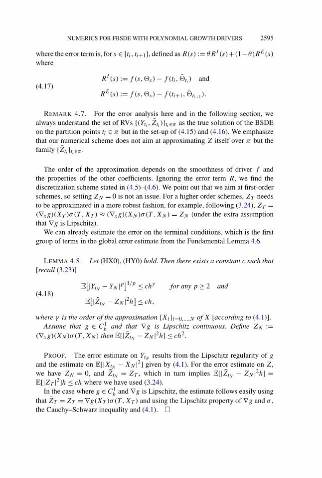
where the error term is, for s ∈ [ti , ti+1], defined as R(s) := θRI (s)+(1−θ)RE(s)
where
RI (s) := f (s,�s) − f (ti, �ti ) and(4.17)
RE(s) := f (s,�s) − f (ti+1, �ti+1).
REMARK 4.7. For the error analysis here and in the following section, wealways understand the set of RVs {(Yti , Zti )}ti∈π as the true solution of the BSDEon the partition points ti ∈ π but in the set-up of (4.15) and (4.16). We emphasizethat our numerical scheme does not aim at approximating Z itself over π but thefamily {Zti }ti∈π .
The order of the approximation depends on the smoothness of driver f andthe properties of the other coefficients. Ignoring the error term R, we find thediscretization scheme stated in (4.5)–(4.6). We point out that we aim at first-orderschemes, so setting ZN = 0 is not an issue. For a higher order schemes, ZT needsto be approximated in a more robust fashion, for example, following (3.24), ZT =(∇xg)(XT )σ (T ,XT ) ≈ (∇xg)(XN)σ(T ,XN) = ZN (under the extra assumptionthat ∇g is Lipschitz).
We can already estimate the error on the terminal conditions, which is the firstgroup of terms in the global error estimate from the Fundamental Lemma 4.6.
LEMMA 4.8. Let (HX0), (HY0) hold. Then there exists a constant c such that[recall (3.23)]
E[|YtN − YN |p]1/p ≤ chγ for any p ≥ 2 and
(4.18)E[|ZtN − ZN |2h]≤ ch,
where γ is the order of the approximation {Xi}i=0,...,N of X [according to (4.1)].Assume that g ∈ C1
b and that ∇g is Lipschitz continuous. Define ZN :=(∇xg)(XN)σ(T ,XN) then E[|ZtN − ZN |2h] ≤ ch2.
PROOF. The error estimate on YtN results from the Lipschitz regularity of g
and the estimate on E[|XtN − XN |2] given by (4.1). For the error estimate on Z,we have ZN = 0, and ZtN = ZT , which in turn implies E[|ZtN − ZN |2h] =E[|ZT |2]h ≤ ch where we have used (3.24).
In the case where g ∈ C1b and ∇g is Lipschitz, the estimate follows easily using
that ZT = ZT = ∇g(XT )σ (T ,XT ) and using the Lipschitz property of ∇g and σ ,the Cauchy–Schwarz inequality and (4.1). �
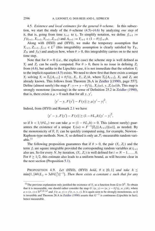
2596 A. LIONNET, G. DOS REIS AND L. SZPRUCH
4.5. Existence and local estimates for the general θ -scheme. In this subsec-tion, we start the study of the θ -scheme (4.5)–(4.6) by analyzing one step ofit, that is, going from time ti+1 to ti . To simplify notation, we define fi+1 :=f (ti+1,Xi+1, Yi+1,Zi+1) and Ai+1 := Yi+1 + (1 − θ)fi+1h.
Along with (HX0) and (HY0), we make the temporary assumption thatYi+1,Zi+1, fi+1 ∈ L2 (this integrability assumption is clearly satisfied by YN ,ZN and fN ) and analyze how, when θ > 0, this integrability carries on to the nexttime step.
Note that for θ = 0 (i.e., the explicit case) the scheme step is well defined asYi and Zi can be easily computed. For θ > 0, there is no issue in defining Zi
from (4.6), but unlike in the Lipschitz case, it is not immediate that the solution Yi
to the implicit equation (4.5) exists. We need to show first that there exists a uniqueYi solving Yi = Ei[Ai+1] + θf (ti,Xi, Yi,Zi)h, where Ei[Ai+1], Xi and Zi arealready known. This follows from Theorem 26.A in Zeidler [(1990), page 557].Define (almost surely) the map F :y �→ y − θf (ti,Xi(ω), y,Zi(ω))h. This map isstrongly monotone (increasing) in the sense of Definition 25.2 in Zeidler (1990),that is, there exists a μ > 0 such that for all y, y′,⟨
y′ − y,F(y′)− F(y)
⟩≥ μ∣∣y′ − y
∣∣2.Indeed, from (HY0) and Remark 2.1 we have⟨
y′ − y,F(y′)− F(y)
⟩≥ (1 − θLyh)∣∣y′ − y
∣∣2,so if h < 1/(θLy) we can take μ = (1 − θLyh) > 0. This (almost surely) guar-antees the existence of a unique Yi(ω) = F−1[Ei[(Ai+1)](ω)], as needed. Bythe monotonicity of F, Yi can be quickly computed using, for example, Newton–Raphson-type methods. Now, Yi so defined is only an Fi-measurable random vari-able.11
The following proposition guarantees that if θ > 0, the pair (Yi,Zi) and theterm fi are square integrable provided the corresponding random variables at ti+1also are. So for every N , by iteration, (Yi,Zi) is well defined for i = N − 1, . . . ,0.For θ ≥ 1/2, this estimate also leads to a uniform bound, as will become clear inthe next section (Proposition 5.1).
PROPOSITION 4.9. Let (HX0), (HY0) hold, θ ∈ [0,1] and take h ≤min{1, [4θ(Ly + 3dθL2
z)]−1}. Then there exists a constant c such that for any
11The previous explanation only justified the existence of Yi as a function from � to Rk . To obtain
that it is measurable, one should rather consider the map G : (a, y) �→ (a, y − θf (ti , a, y)h), wherea = (x, z) ∈ R
d×k×d and f (t, a, y) = f (t, x, y, z). It is again seen to be strongly monotonous, so itis invertible and Theorem 26.A in Zeidler (1990) asserts that G−1 is continuous (Lipschitz in fact),hence measurable.
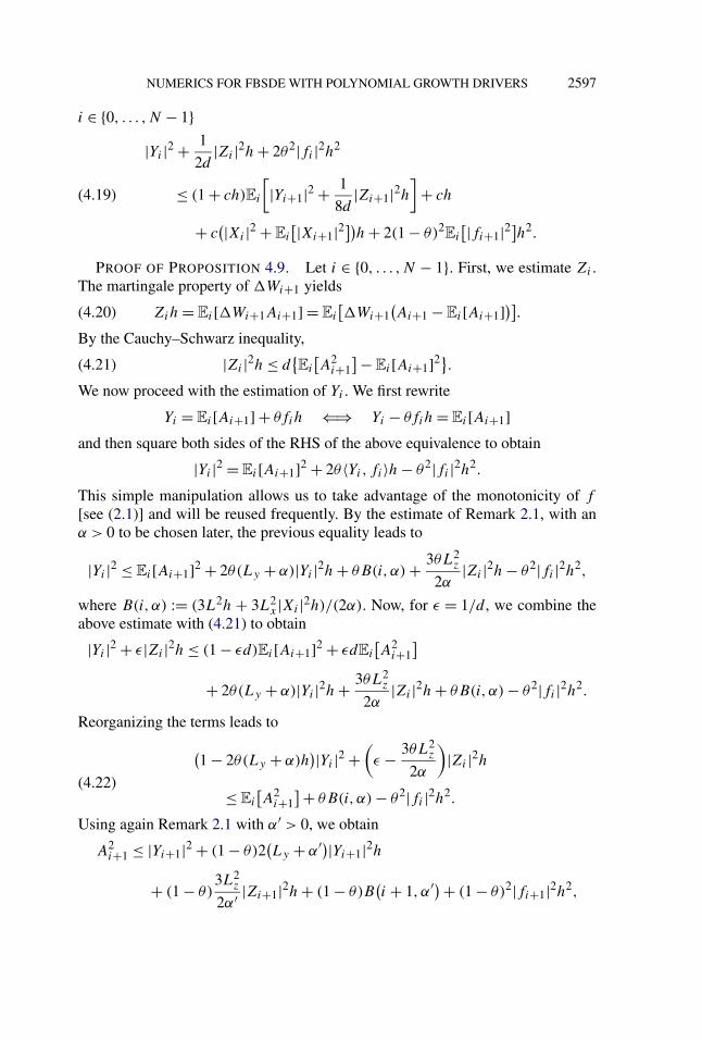
NUMERICS FOR FBSDE WITH POLYNOMIAL GROWTH DRIVERS 2597
i ∈ {0, . . . ,N − 1}|Yi |2 + 1
2d|Zi |2h + 2θ2|fi |2h2
≤ (1 + ch)Ei
[|Yi+1|2 + 1
8d|Zi+1|2h
]+ ch(4.19)
+ c(|Xi |2 +Ei
[|Xi+1|2])h + 2(1 − θ)2Ei
[|fi+1|2]h2.
PROOF OF PROPOSITION 4.9. Let i ∈ {0, . . . ,N − 1}. First, we estimate Zi .The martingale property of Wi+1 yields
Zih = Ei[Wi+1Ai+1] = Ei
[Wi+1
(Ai+1 −Ei[Ai+1])].(4.20)
By the Cauchy–Schwarz inequality,
|Zi |2h ≤ d{Ei
[A2
i+1]−Ei[Ai+1]2}.(4.21)
We now proceed with the estimation of Yi . We first rewrite
Yi = Ei[Ai+1] + θfih ⇐⇒ Yi − θfih = Ei[Ai+1]and then square both sides of the RHS of the above equivalence to obtain
|Yi |2 = Ei[Ai+1]2 + 2θ〈Yi, fi〉h − θ2|fi |2h2.
This simple manipulation allows us to take advantage of the monotonicity of f
[see (2.1)] and will be reused frequently. By the estimate of Remark 2.1, with anα > 0 to be chosen later, the previous equality leads to
|Yi |2 ≤ Ei[Ai+1]2 + 2θ(Ly + α)|Yi |2h + θB(i, α) + 3θL2z
2α|Zi |2h − θ2|fi |2h2,
where B(i,α) := (3L2h + 3L2x |Xi |2h)/(2α). Now, for ε = 1/d , we combine the
above estimate with (4.21) to obtain
|Yi |2 + ε|Zi |2h ≤ (1 − εd)Ei[Ai+1]2 + εdEi
[A2
i+1]
+ 2θ(Ly + α)|Yi |2h + 3θL2z
2α|Zi |2h + θB(i, α) − θ2|fi |2h2.
Reorganizing the terms leads to(1 − 2θ(Ly + α)h
)|Yi |2 +(ε − 3θL2
z
2α
)|Zi |2h
(4.22)≤ Ei
[A2
i+1]+ θB(i, α) − θ2|fi |2h2.
Using again Remark 2.1 with α′ > 0, we obtain
A2i+1 ≤ |Yi+1|2 + (1 − θ)2
(Ly + α′)|Yi+1|2h
+ (1 − θ)3L2
z
2α′ |Zi+1|2h + (1 − θ)B(i + 1, α′)+ (1 − θ)2|fi+1|2h2,
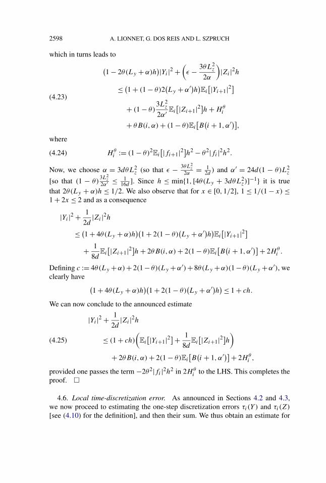
2598 A. LIONNET, G. DOS REIS AND L. SZPRUCH
which in turns leads to(1 − 2θ(Ly + α)h
)|Yi |2 +(ε − 3θL2
z
2α
)|Zi |2h
≤ (1 + (1 − θ)2
(Ly + α′)h)Ei
[|Yi+1|2](4.23)
+ (1 − θ)3L2
z
2α′ Ei
[|Zi+1|2]h + Hθi
+ θB(i, α) + (1 − θ)Ei
[B(i + 1, α′)],
where
Hθi := (1 − θ)2
Ei
[|fi+1|2]h2 − θ2|fi |2h2.(4.24)
Now, we choose α = 3dθL2z (so that ε − 3θL2
z
2α= 1
2d) and α′ = 24d(1 − θ)L2
z
[so that (1 − θ)3L2
z
2α′ ≤ 116d
]. Since h ≤ min{1, [4θ(Ly + 3dθL2z)]−1} it is true
that 2θ(Ly + α)h ≤ 1/2. We also observe that for x ∈ [0,1/2], 1 ≤ 1/(1 − x) ≤1 + 2x ≤ 2 and as a consequence
|Yi |2 + 1
2d|Zi |2h
≤ (1 + 4θ(Ly + α)h
)(1 + 2(1 − θ)
(Ly + α′)h)Ei
[|Yi+1|2]+ 1
8dEi
[|Zi+1|2]h + 2θB(i, α) + 2(1 − θ)Ei
[B(i + 1, α′)]+ 2Hθ
i .
Defining c := 4θ(Ly +α)+ 2(1 − θ)(Ly +α′)+ 8θ(Ly +α)(1 − θ)(Ly +α′), weclearly have (
1 + 4θ(Ly + α)h)(
1 + 2(1 − θ)(Ly + α′)h)≤ 1 + ch.
We can now conclude to the announced estimate
|Yi |2 + 1
2d|Zi |2h
≤ (1 + ch)
(Ei
[|Yi+1|2]+ 1
8dEi
[|Zi+1|2]h)(4.25)
+ 2θB(i, α) + 2(1 − θ)Ei
[B(i + 1, α′)]+ 2Hθ
i ,
provided one passes the term −2θ2|fi |2h2 in 2Hθi to the LHS. This completes the
proof. �
4.6. Local time-discretization error. As announced in Sections 4.2 and 4.3,we now proceed to estimating the one-step discretization errors τi(Y ) and τi(Z)
[see (4.10) for the definition], and then their sum. We thus obtain an estimate for
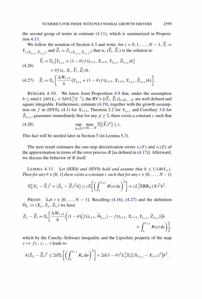
NUMERICS FOR FBSDE WITH POLYNOMIAL GROWTH DRIVERS 2599
the second group of terms in estimate (4.11), which is summarized in Proposi-tion 4.13.
We follow the notation of Section 4.3 and write, for i = 0,1, . . . ,N − 1, Yi =Yi,(Yti+1 ,Zti+1 ) and Zi = Zi,(Yti+1 ,Zti+1 ); that is, (Yi, Zi) is the solution to
Yi = Eti
[Yti+1 + (1 − θ)f (ti+1,Xi+1, Yti+1, Zti+1)h
](4.26)
+ θf (ti,Xi, Yi, Zi)h,
Zi = Eti
[Wi+1
h
(Yti+1 + (1 − θ)f (ti+1,Xi+1, Yti+1, Zti+1)h
)].(4.27)
REMARK 4.10. We know from Proposition 4.9 that, under the assumptionh ≤ min{1, [4θ(Ly +3dθL2
z)]−1}, the RV’s {(Yi , Zi)}i=0,...,N are well defined andsquare integrable. Furthermore, estimate (4.19), together with the growth assump-tion on f in (HY0), (4.1) for Xi+1, Theorem 2.2 for Yti+1 and Corollary 3.6 forZti+1 , guarantee immediately that for any p ≥ 2, there exists a constant c such that
supN∈N
maxi=0,...,N
E[|Yi |p]≤ c.(4.28)
This fact will be needed later in Section 5 (in Lemma 5.3).
The next result estimates the one-step discretization errors τi(Y ) and τi(Z) ofthe approximation in terms of the error process R [as defined in (4.17)]. Afterward,we discuss the behavior of R itself.
LEMMA 4.11. Let (HX0) and (HY0) hold and assume that h ≤ 1/(4θLy).Then for any θ ∈ [0,1] there exists a constant c such that for any i ∈ {0, . . . ,N −1}
E[|Yti − Yi |2 + |Zti − Zi |2h]≤ cE
[(∫ ti+1
ti
R(s)ds
)2]+ cL2
xERRπ(X)2h2.
PROOF. Let i ∈ {0, . . . ,N − 1}. Recalling (4.16), (4.27) and the definition�ti := (Xti , Yti , Zti ) we have
Zti − Zi = Ei
[Wi+1
h
((1 − θ)
[f (ti+1, �ti+1) − f (ti+1,Xi+1, Yti+1, Zti+1)
]h
+∫ ti+1
ti
R(s)ds
)],
which by the Cauchy–Schwarz inequality and the Lipschitz property of the mapx �→ f (·, x, ·, ·) leads to
h|Zti − Zi |2 ≤ 2dEi
[(∫ ti+1
ti
Ru du
)2]+ 2d(1 − θ)2L2
xEi
[|Xti+1 − Xi+1|2]h2.
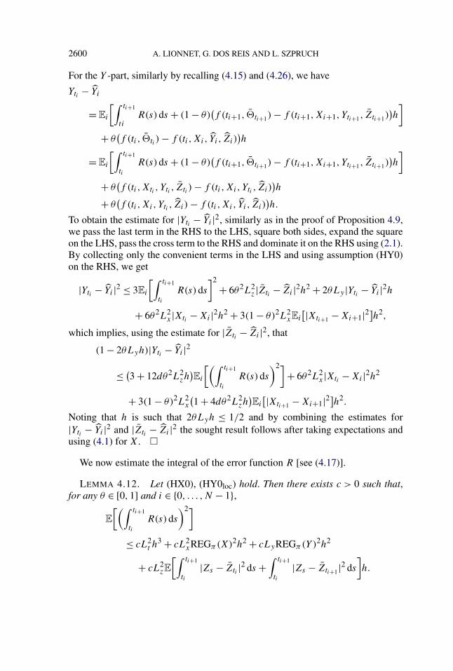
2600 A. LIONNET, G. DOS REIS AND L. SZPRUCH
For the Y -part, similarly by recalling (4.15) and (4.26), we have
Yti − Yi
= Ei
[∫ ti+1
t iR(s)ds + (1 − θ)
(f (ti+1, �ti+1) − f (ti+1,Xi+1, Yti+1, Zti+1)
)h
]+ θ
(f (ti, �ti ) − f (ti,Xi, Yi, Zi)
)h
= Ei
[∫ ti+1
ti
R(s)ds + (1 − θ)(f (ti+1, �ti+1) − f (ti+1,Xi+1, Yti+1, Zti+1)
)h
]+ θ
(f (ti,Xti , Yti , Zti ) − f (ti,Xi, Yti , Zi)
)h
+ θ(f (ti,Xi, Yti , Zi) − f (ti,Xi, Yi, Zi)
)h.
To obtain the estimate for |Yti − Yi |2, similarly as in the proof of Proposition 4.9,we pass the last term in the RHS to the LHS, square both sides, expand the squareon the LHS, pass the cross term to the RHS and dominate it on the RHS using (2.1).By collecting only the convenient terms in the LHS and using assumption (HY0)on the RHS, we get
|Yti − Yi |2 ≤ 3Ei
[∫ ti+1
ti
R(s)ds
]2
+ 6θ2L2z|Zti − Zi |2h2 + 2θLy |Yti − Yi |2h
+ 6θ2L2x |Xti − Xi |2h2 + 3(1 − θ)2L2
xEi
[|Xti+1 − Xi+1|2]h2,
which implies, using the estimate for |Zti − Zi |2, that
(1 − 2θLyh)|Yti − Yi |2
≤ (3 + 12dθ2L2
zh)Ei
[(∫ ti+1
ti
R(s)ds
)2]+ 6θ2L2
x |Xti − Xi |2h2
+ 3(1 − θ)2L2x
(1 + 4dθ2L2
zh)Ei
[|Xti+1 − Xi+1|2]h2.
Noting that h is such that 2θLyh ≤ 1/2 and by combining the estimates for|Yti − Yi |2 and |Zti − Zi |2 the sought result follows after taking expectations andusing (4.1) for X. �
We now estimate the integral of the error function R [see (4.17)].
LEMMA 4.12. Let (HX0), (HY0loc) hold. Then there exists c > 0 such that,for any θ ∈ [0,1] and i ∈ {0, . . . ,N − 1},
E
[(∫ ti+1
ti
R(s)ds
)2]≤ cL2
t h3 + cL2
xREGπ(X)2h2 + cLyREGπ(Y )2h2
+ cL2zE
[∫ ti+1
ti
|Zs − Zti |2 ds +∫ ti+1
ti
|Zs − Zti+1 |2 ds
]h.
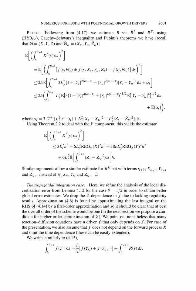
NUMERICS FOR FBSDE WITH POLYNOMIAL GROWTH DRIVERS 2601
PROOF. Following from (4.17), we estimate R via RI and RE : using(HY0loc), Cauchy–Schwarz’s inequality and Fubini’s theorems we have [recallthat � = (X,Y,Z) and �ti = (Xti , Yti , Zti )]
E
[(∫ ti+1
ti
RI (s)ds
)2]
= E
[(∫ ti+1
ti
[f (s,�s) ± f (s,Xs,Yti ,Zs) − f (ti, �ti )
]ds
)2]
≤ 2hE
[∫ ti+1
ti
3L2y
(1 + |Ys |2(m−1) + |Yti |2(m−1))|Ys − Yti |2 ds + αi
]
≤ 2h
(∫ ti+1
ti
L2yE[3(1 + |Ys |4(m−1) + |Yti |4(m−1))]1/2
E[|Ys − Yti |4
]1/2 ds
+E[αi]),
where αi = 3∫ ti+1ti
[L2t |s − ti | + L2
x |Xs − Xti |2 + L2z|Zs − Zti |2]ds.
Using Theorem 2.2 to deal with the Y component, this yields the estimate
E
[(∫ ti+1
ti
RI (s)ds
)2]≤ 3L2
t h3 + 6L2
xREGπ(X)2h2 + 18cL2yREGπ(Y )2h2
+ 6L2zE
[∫ ti+1
ti
|Zs − Zti |2 ds
]h.
Similar arguments allow a similar estimate for RE but with terms ti+1, Xti+1 , Yti+1
and Zti+1 instead of ti , Xti , Yti and Zti . �
The trapezoidal integration case. Here, we refine the analysis of the local dis-cretization error from Lemma 4.12 for the case θ = 1/2 in order to obtain betterglobal error estimates. We drop the Z-dependence in f due to lacking regularityresults. Approximation (4.6) is found by approximating the last integral on theRHS of (4.14) by a first-order approximation and so it should be clear that at bestthe overall order of the scheme would be one (in the next section we propose a can-didate for higher order approximation of Z). We point out nonetheless that manyreaction–diffusion equations have a driver f that only depends on Y . For ease ofthe presentation, we also assume that f does not depend on the forward process X
and omit the time dependence (these can be easily extended).We write, similarly to (4.15),∫ ti+1
ti
f (Ys)ds = h
2
[f (Yti ) + f (Yti+1)
]+ ∫ ti+1
ti
R(s)ds,
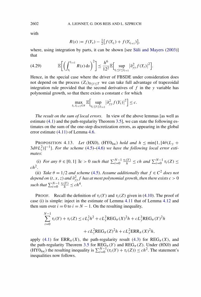
2602 A. LIONNET, G. DOS REIS AND L. SZPRUCH
with
R(s) := f (Ys) − 12
[f (Yti ) + f (Yti+1)
],
where, using integration by parts, it can be shown [see Süli and Mayers (2003)]that
E
[(∫ ti+1
ti
R(s)ds
)2]≤ h6
122E[
supti≤t≤ti+1
∣∣∂2yyf (Yt )
∣∣2].(4.29)
Hence, in the special case where the driver of FBSDE under consideration doesnot depend on the process (Zt )0≤t≤T we can take full advantage of trapezoidalintegration rule provided that the second derivatives of f in the y variable haspolynomial growth, so that there exists a constant c for which
maxti ,ti+1∈π
E
[sup
ti≤t≤ti+1
∣∣∂2yyf (Yt )
∣∣2]≤ c.
The result on the sum of local errors. In view of the above lemmas [as well asestimate (4.1) and the path-regularity Theorem 3.5], we can state the following es-timates on the sum of the one-step discretization errors, as appearing in the globalerror estimate (4.11) of Lemma 4.6.
PROPOSITION 4.13. Let (HX0), (HY0loc) hold and h ≤ min{1, [4θ(Ly +3dθL2
z)]−1}. For the scheme (4.5)–(4.6) we have the following local error esti-mates:
(i) For any θ ∈ [0,1] ∃c > 0 such that∑N−1
i=0τi (Y )
h≤ ch and
∑N−1i=0 τi(Z) ≤
ch2.(ii) Take θ = 1/2 and scheme (4.5). Assume additionally that f ∈ C2 does not
depend on (t, x, z) and ∂2yyf has at most polynomial growth, then there exists c > 0
such that∑N−1
i=0τi (Y )
h≤ ch4.
PROOF. Recall the definition of τi(Y ) and τi(Z) given in (4.10). The proof ofcase (i) is simple: inject in the estimate of Lemma 4.11 that of Lemma 4.12 andthen sum over i = 0 to i = N − 1. On the resulting inequality,
N−1∑i=0
τi(Y ) + τi(Z) ≤ cL2t h
2 + cL2xREGπ(X)2h + cL2
yREGπ(Y )2h
+ cL2zREGπ(Z)2h + cL2
xERRπ(X)2h,
apply (4.1) for ERRπ(X), the path-regularity result (4.3) for REGπ(X), andthe path-regularity Theorem 3.5 for REGπ(Y ) and REGπ(Z). Under (HX0) and(HY0loc) the resulting inequality is
∑N−1i=0 (τi(Y ) + τi(Z)) ≤ ch2. The statement’s
inequalities now follows.
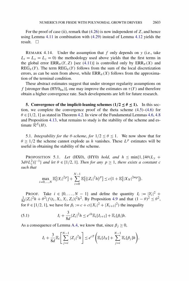
NUMERICS FOR FBSDE WITH POLYNOMIAL GROWTH DRIVERS 2603
For the proof of case (ii), remark that (4.26) is now independent of Z, and henceusing Lemma 4.11 in combination with (4.29) instead of Lemma 4.12 yields theresult. �
REMARK 4.14. Under the assumption that f only depends on y (i.e., takeLt = Lx = Lz = 0) the methodology used above yields that the first terms inthe global error ERRπ(Y,Z) [see (4.11)] is controlled only by ERRπ(X) andREGπ(Y ). The term REGπ(Y ) follows from the sum of the local discretizationerrors, as can be seen from above, while ERRπ(X) follows from the approxima-tion of the terminal condition.
These abstract estimates suggest that under stronger regularity assumptions onf [stronger than (HY0loc)], one may improve the estimates on τ(Y ) and thereforeobtain a higher convergence rate. Such developments are left for future research.
5. Convergence of the implicit-leaning schemes (1/2 ≤ θ ≤ 1). In this sec-tion, we complete the convergence proof of the theta scheme (4.5)–(4.6) forθ ∈ [1/2,1] as stated in Theorem 4.2. In view of the Fundamental Lemmas 4.6, 4.8and Proposition 4.13, what remains to study is the stability of the scheme and es-timate RS(H).
5.1. Integrability for the θ -scheme, for 1/2 ≤ θ ≤ 1. We now show that forθ ≥ 1/2 the scheme cannot explode as h vanishes. These Lp estimates will beuseful in obtaining the stability of the scheme.
PROPOSITION 5.1. Let (HX0), (HY0) hold, and h ≤ min{1, [4θ(Ly +3dθL2
z)]−1} and let θ ∈ [1/2,1]. Then for any p ≥ 1, there exists a constant c
such that
maxi=0,...,N
E[|Yi |2p]+ N−1∑
i=0
E[(|Zi |2h)p]≤ c
(1 +E
[|XN |2mp]).PROOF. Take i ∈ {0, . . . ,N − 1} and define the quantity Ii := |Yi |2 +
18d
|Zi |2h + θ2|f (ti,Xi, Yi,Zi)|2h2. By Proposition 4.9 and that (1 − θ)2 ≤ θ2,
for θ ∈ [1/2,1], we have for βi := c + c(|Xi |2 + |Xi+1|2) the inequality
Ii + 3
8d|Zi |2h ≤ ech
Ei[Ii+1] +Ei[βi]h.(5.1)
As a consequence of Lemma A.4, we know that, since βj ≥ 0,
Ii + 3
8dEi
[N−1∑j=i
|Zj |2h]
≤ ecT
(Ei[IN ] +
N−1∑j=i
Ei[βj ]h),
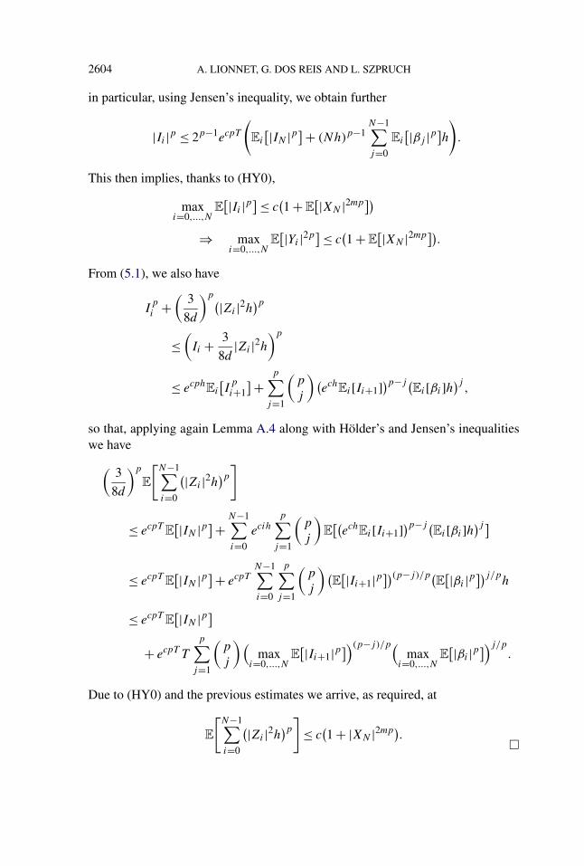
2604 A. LIONNET, G. DOS REIS AND L. SZPRUCH
in particular, using Jensen’s inequality, we obtain further
|Ii |p ≤ 2p−1ecpT
(Ei
[|IN |p]+ (Nh)p−1N−1∑j=0
Ei
[|βj |p]h).
This then implies, thanks to (HY0),
maxi=0,...,N
E[|Ii |p]≤ c
(1 +E
[|XN |2mp])⇒ max
i=0,...,NE[|Yi |2p]≤ c
(1 +E
[|XN |2mp]).From (5.1), we also have
Ipi +
(3
8d
)p(|Zi |2h)p≤(Ii + 3
8d|Zi |2h
)p
≤ ecphEi
[I
pi+1
]+ p∑j=1
(p
j
)(ech
Ei[Ii+1])p−j (Ei[βi]h)j ,
so that, applying again Lemma A.4 along with Hölder’s and Jensen’s inequalitieswe have(
3
8d
)p
E
[N−1∑i=0
(|Zi |2h)p]
≤ ecpTE[|IN |p]+ N−1∑
i=0
ecihp∑
j=1
(p
j
)E[(
echEi[Ii+1])p−j (
Ei[βi]h)j ]
≤ ecpTE[|IN |p]+ ecpT
N−1∑i=0
p∑j=1
(p
j
)(E[|Ii+1|p])(p−j)/p(
E[|βi |p])j/p
h
≤ ecpTE[|IN |p]
+ ecpT T
p∑j=1
(p
j
)(max
i=0,...,NE[|Ii+1|p])(p−j)/p(
maxi=0,...,N
E[|βi |p])j/p
.
Due to (HY0) and the previous estimates we arrive, as required, at
E
[N−1∑i=0
(|Zi |2h)p]
≤ c(1 + |XN |2mp).
�
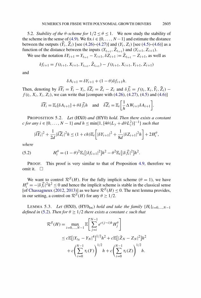
NUMERICS FOR FBSDE WITH POLYNOMIAL GROWTH DRIVERS 2605
5.2. Stability of the θ -scheme for 1/2 ≤ θ ≤ 1. We now study the stability ofthe scheme in the sense of (4.9). We fix i ∈ {0, . . . ,N −1} and estimate the distancebetween the outputs (Yi, Zi) [see (4.26)–(4.27)] and (Yi,Zi) [see (4.5)–(4.6)] as afunction of the distance between the inputs (Yti+1, Zti+1) and (Yi+1,Zi+1).
We use the notation δYi+1 = Yti+1 − Yi+1, δZi+1 := Zti+1 − Zi+1, as well as
δfi+1 = f (ti+1,Xi+1, Yti+1, Zti+1) − f (ti+1,Xi+1, Yi+1,Zi+1)
and
δAi+1 = δYi+1 + (1 − θ)δfi+1h.
Then, denoting by δYi = Yi − Yi , δZi = Zi − Zi and δfi = f (ti,Xi, Yi , Zi) −f (ti,Xi, Yi,Zi), we can write that [compare with (4.26), (4.27), (4.5) and (4.6)]
δYi = Ei[δAi+1] + θδfih and δZi = Ei
[1
hWi+1δAi+1
].
PROPOSITION 5.2. Let (HX0) and (HY0) hold. Then there exists a constantc for any i ∈ {0, . . . ,N − 1} and h ≤ min{1, [4θ(Ly + dθL2
z)]−1} such that
|δYi |2 + 1
2d|δZi |2h ≤ (1 + ch)Ei
[|δYi+1|2 + 1
8d|δZi+1|2h
]+ 2Hθ
i ,
where
Hθi = (1 − θ)2
Ei
[|δfi+1|2]h2 − θ2Ei
[|δfi |2]h2.(5.2)
PROOF. This proof is very similar to that of Proposition 4.9, therefore weomit it. �
We want to control RS(H). For the fully implicit scheme (θ = 1), we haveHθ
i = −|δfi |2h2 ≤ 0 and hence the implicit scheme is stable in the classical sense[of Chassagneux (2012, 2013)] as we have RS(H) ≤ 0. The next lemma provides,in our setting, a control on RS(H) for any θ ≥ 1/2.
LEMMA 5.3. Let (HX0), (HY0loc) hold and take the family {Hi}i=0,...,N−1defined in (5.2). Then for θ ≥ 1/2 there exists a constant c such that
RS(H) = maxi=0,...,N−1
E
[N−1∑j=i
ec(j−i)hHθj
]
≤ cE[|YtN − YN |4]1/2
h2 + cE[|ZN − ZN |2]h2
+ c
(N−1∑i=0
τi(Y )
)1/2
h + c
(N−1∑i=0
τi(Z)
)1/2
h.
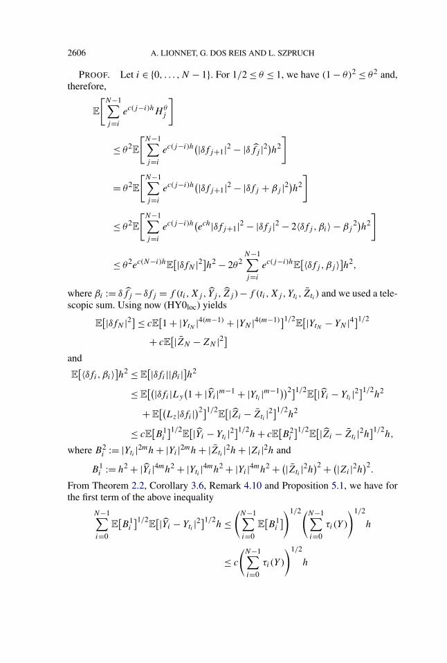
2606 A. LIONNET, G. DOS REIS AND L. SZPRUCH
PROOF. Let i ∈ {0, . . . ,N − 1}. For 1/2 ≤ θ ≤ 1, we have (1 − θ)2 ≤ θ2 and,therefore,
E
[N−1∑j=i
ec(j−i)hHθj
]
≤ θ2E
[N−1∑j=i
ec(j−i)h(|δfj+1|2 − |δfj |2)h2
]
= θ2E
[N−1∑j=i
ec(j−i)h(|δfj+1|2 − |δfj + βj |2)h2
]
≤ θ2E
[N−1∑j=i
ec(j−i)h(ech|δfj+1|2 − |δfj |2 − 2〈δfj , βi〉 − βj2)h2
]
≤ θ2ec(N−i)hE[|δfN |2]h2 − 2θ2
N−1∑j=i
ec(j−i)hE[〈δfj , βj 〉]h2,
where βi := δfj − δfj = f (ti,Xj , Yj , Zj )−f (ti,Xj ,Yti , Zti ) and we used a tele-scopic sum. Using now (HY0loc) yields
E[|δfN |2]≤ cE
[1 + |YtN |4(m−1) + |YN |4(m−1)]1/2
E[|YtN − YN |4]1/2
+ cE[|ZN − ZN |2]
and
E[〈δfi, βi〉]h2 ≤ E
[|δfi ||βi |]h2
≤ E[(|δfi |Ly
(1 + |Yi |m−1 + |Yti |m−1))2]1/2
E[|Yi − Yti |2
]1/2h2
+E[(
Lz|δfi |)2]1/2E[|Zi − Zti |2
]1/2h2
≤ cE[B1
i
]1/2E[|Yi − Yti |2
]1/2h + cE
[B2
i
]1/2E[|Zi − Zti |2h
]1/2h,
where B2i := |Yti |2mh + |Yi |2mh + |Zti |2h + |Zi |2h and
B1i := h2 + |Yi |4mh2 + |Yti |4mh2 + |Yi |4mh2 + (|Zti |2h
)2 + (|Zi |2h)2.From Theorem 2.2, Corollary 3.6, Remark 4.10 and Proposition 5.1, we have forthe first term of the above inequality
N−1∑i=0
E[B1
i
]1/2E[|Yi − Yti |2
]1/2h ≤
(N−1∑i=0
E[B1
i
])1/2(N−1∑i=0
τi(Y )
)1/2
h
≤ c
(N−1∑i=0
τi(Y )
)1/2
h
NUMERICS FOR FBSDE WITH POLYNOMIAL GROWTH DRIVERS 2607
and similarly for the second term
N−1∑i=0
E[B2
i
]1/2E[|Zi − Zti |2h
]1/2h ≤ c
(N−1∑i=0
τi(Z)
)1/2
h.�
5.3. Convergence of the scheme. By collecting the above results, we can nowprove Theorem 4.2.
PROOF OF THEOREM 4.2. The proof is a combination of the FundamentalLemmas 4.6 and 4.8, Proposition 4.13 and stability results obtained in this section,namely Proposition 5.2 and Lemma 5.3.
We move to the proof of part (ii), the case θ = 1/2. Since in this case f dependsonly on y, a quick rerun of arguments of the Fundamental Lemma 4.6, shows thereexists a constant c > 0 such that
maxi=0,...,N
E[|Yti − Yi |2]≤ c
{E[|YtN − YN |2]+ N−1∑
i=0
τi(Y )
h
}+ (1 + h)RS(H).
The first two terms on the RHS can be bounded by ch2γ + ch4, c > 0, usingLemma 4.8 and Proposition 4.13, respectively. By Lemma 5.3, there exists a con-stant c > 0 such that
RS(H) ≤ cE[|YtN − YN |4]1/2
h2 + c
(N−1∑i=0
τi(Y )
)1/2
h,
and using again Lemma 4.8 and Proposition 4.13 yields RS(H) ≤ ch2γ+2 +ch7/2.By joining these results, the theorem’s conclusion follows. �
5.4. Further remarks. Here, we discuss a true overall second-order scheme,namely a second-order discretization for Z and an intuitive variance reductiontechnique which we have used throughout but not made formally explicit.
5.4.1. The candidate for second-order scheme. For the general case where thedriver depends on Z, the approximation for Zi , namely (4.6), is not enough to ob-tain a higher order scheme as it is a first-order approximation. The proper higherorder scheme in its full generality follows by applying the trapezoidal rule to all in-tegrals present in (4.14); as is done for (4.13). With some manipulation (left to thereader), we end up with the following approximation for Zi [compare with (4.6)]:
Zi = 2
hEi
[Wi+1
(Yti+1 + (1 − θ)f (ti,Xi+1, Yi+1,Zi+1)h
)]−Ei[Zi+1],with θ = 1/2, the terminal condition YN = g(XN), along with (4.5) and a suitableapproximation for ZT . An approximation for ZT is not trivial and could, for in-stance, be found via Malliavin calculus. The general treatment of such a scheme isleft for future research.
2608 A. LIONNET, G. DOS REIS AND L. SZPRUCH
Another type of second-order scheme can be found in Crisan and Manolarakis(2010); the approximation there is based on Itô–Taylor expansions.
5.4.2. Controlling the variance of the scheme. If we use the notation set up inSection 4.5, the approximation (4.6) can be written out as Zi = Ei[Wi+1Ai+1]/h.We point out that implementation-wise it is better to use the lower variance approx-imation (4.20) instead of (4.6), that is, to use
Zi = 1
hEi
[Wi+1
(Ai+1 −Ei[Ai+1])], i = 0, . . . ,N − 1.
This does not lead to a relevant additional computation effort, as Ei[Ai+1] mustbe computed for the estimation of the Yi component. To avoid a long analysis,we make some simplifying assumptions in order to better explain the gain: as-sume Xt = x + Wt and that we are about to compute Z0 (a standard expec-tation); assume further (via Doob–Dynkin lemma) that A1 can be written as12
A1 = ϕ(X1) = ϕ(x + W1) where ϕ has some regularity so that
ϕ(x + W1) = ϕ(x) + ϕ′(x)(W1) + 12ϕ′′(x∗)(W1)
2,
where x∗ lies between x and x + W1. Then the Monte Carlo (MC) estimatorfor Z0 from (4.6), with M samples of the normal N (0,1) distribution given by{N λ}λ=1,...,M , and its standard deviation (St.d.) are
ZMC,(4.6)0 = 1
M
M∑λ=1
√hN λ
hϕ(x + √
hN λ) with St.d. ≈ |ϕ(x)|√h√
M.
Using (4.20) instead of (4.6) to compute Z0 would produce the MC estimator andits St.d.
ZMC,(4.20)0 = 1
M
M∑λ=1
√hN λ
h
(ϕ(x + √
hN λ)− ϕ(x))
with St.d. ≈ |ϕ′(x)|√M
.
Compare now the standard deviation of both estimators. It is crucial for the stabilitythat the denominator of the variance of Z
MC,(4.20)0 lacks that
√h term. If M is
kept fixed then as h gets smaller we expect ZMC,(4.6)0 to blow up while Z
MC,(4.20)0
will remain controlled (assuming ϕ can be controlled13). This can be numericallyconfirmed in Alanko and Avellaneda (2013).
We point out that this simple trick can be adapted to the scheme proposed in thenext section as well as to the computation of the second-order scheme proposedpreviously.
12If the reader is aware of how conditional expectations in the BSDE framework are calculated, say,for example, via projection over a basis of functions, having a function ϕ is expected.
13In Gobet and Turkedjiev (2011), it is shown for the locally Lipschitz driver case that ϕ is indeeda Lipschitz function of its variables.
NUMERICS FOR FBSDE WITH POLYNOMIAL GROWTH DRIVERS 2609
6. Convergence of the tamed explicit scheme. We now turn our attentionback to the explicit scheme. Unlike the case θ ∈ [1/2,1], when θ < 1/2, the localestimates of Proposition 4.9 cannot be extended to the global ones (as in Proposi-tion 5.1). Consequently, we also do not have a control over the stability remainderRS(H) (see Definition 4.4). In fact, as the motivating example of the Introductionshows, the scheme can explode. To remedy to this, we consider the tamed explicitscheme, described in (4.7)–(4.8), which in turn corresponds to a truncation pro-cedure applied to the original BSDE, and show that this scheme converges. Ouranalysis yields as a by-product sufficient conditions under which the naive explicitscheme converges (see Remark 6.6).
REMARK 6.1 (m > 1). In this section, we focus exclusively on the case m > 1in assumption (HY0). The easier case m = 1 does not require taming and stabilityof the scheme results from a straightforward adaptation of the proof of Proposi-tion 6.4.
6.1. Principle. The idea is that with the truncation functions TLhand TKh
[re-call the scheme (4.7)–(4.8)], one cannot only obtain uniform integrability boundsfor the scheme, but also a pathwise bound, ensuring that the output {Yi}i=0,...,N
stays under a certain threshold, under which the scheme is found to be stable in thesense of (4.9) with Hi = 0.
Note that this tamed scheme is not exactly the scheme (4.5)–(4.6) with θ = 0.However, it can be seen as the case θ = 0 with the functions TLh
◦ g andf (·, TKh
(·), ·, ·) instead of g and f . They satisfy the same properties with the sameconstants, so we can reuse the results of Section 4.
Because the scheme is controlled, we naturally compare first its output{(Yi,Zi)}i∈{0,...,N} to (Y ′
ti, Z′
ti)ti∈π , where (Y ′
t ,Z′t )t∈[0,T ] is the solution to the
BSDE (1.2) with controlled coefficients, for t ∈ [0, T ]
Y ′t = TLh
(g(XT )
)+ ∫ T
tf(u,TKh
(Xu),Y′u,Z
′u
)du −
∫ T
tZ′
u dWu.(6.1)
This part of analysis follows the methodology used above.In a second step, it is enough to estimate the distance between the solution
(Y ′,Z′) of the truncated BSDE (6.1) and the solution (Y,Z) of the originalBSDE (1.2) in order to conclude to the convergence of the scheme.
In line with Sections 4 and 5, we define {Z′ti}ti∈π as in (3.23), Yi = Yi,(Y ′
i+1,Z′i+1)
and Zi = Zi,(Y ′i+1,Z
′i+1)
for i = 0, . . . ,N − 1, more precisely
Yi := Ei
[Y ′
ti+1+ f
(ti+1, TKh
(Xi+1), Y′ti+1
, Z′ti+1
)h],(6.2)
Zi := Ei
[Wi+1
h
(Y ′
ti+1+ fh
(ti+1,Xi+1, Y
′ti+1
, Z′ti+1
)h)]
.(6.3)
2610 A. LIONNET, G. DOS REIS AND L. SZPRUCH
6.2. Integrability for the scheme. We now show that the tamed Euler schemehas the property that |Yi | ≤ h−1/(2m−2) for all i ∈ {0, . . . ,N}. This is already truefor YN = TLh
(g(XN)) by construction. In the next two propositions, we will showthat this bound propagates through time.
PROPOSITION 6.2. Assume (HX0), (HY0) and that h ≤ 1/(32dL2z). If for a
given i ∈ {0, . . . ,N − 1} one has |Yi+1| ≤ h−1/(2m−2), then one also has
|Yi |2 + 1
d|Zi |2h ≤ (1 + c1h)Ei
[|Yi+1|2 + 1
4d|Zi+1|2h
]+ c2h + c2hEi
[∣∣TKh(Xi+1)
∣∣2].PROOF. Take i ∈ {0, . . . ,N −1}. We have seen in the proof of Proposition 4.9,
equation (4.23) that, since θ = 0,
|Yi |2 + 1
d|Zi |2h ≤ (
1 + 2(Ly + α′)h)Ei
[|Yi+1|2]+ 3L2
z
2α′ Ei
[|Zi+1|2]h +Ei
[B(i + 1, α′)]+ H 0
i ,
where B(i + 1, α′) := (3L2h + 3L2x |TKh
(Xi+1)|2h)/2α′ and
H 0i = Ei
[|fi+1|2]h2 = Ei
[∣∣f (ti+1, TKN(Xi+1), Yi+1,Zi+1
)∣∣2]h2.
Using (HY0) and the fact that |Yi+1|2(m−1)h ≤ 1, we have
|fi+1|2h2 ≤ 4L2h2 + 4L2x
∣∣TKh(Xi+1)
∣∣2h2
+ 4L2y
[|Yi+1|2(m−1)h]|Yi+1|2h + 4L2
z|Zi+1|2h2
≤ 4L2h2 + 4L2x
∣∣TKh(Xi+1)
∣∣2h2 + 4L2y |Yi+1|2h + 4L2
zh|Zi+1|2h,
so we have in the end
|Yi |2 + 1
d|Zi |2h ≤ (
1 + 2(Ly + α′ + 2L2
y
)h)Ei
[|Yi+1|2]+(
3L2z
2α′ + 4L2zh
)Ei
[|Zi+1|2]h+(
3L2
2α′ + 4L2h
)h +
(3L2
x
2α′ + 4L2xh
)Ei
[∣∣TKh(Xi+1)
∣∣2]h.
Choose now α′ = 12dL2z [so that 3L2
z/(2α′) ≤ 1/(8d)] and combine with the re-striction h ≤ 1/(32dL2
z) (so that 4L2zh ≤ 1
8d). Taking c1 = 2(Ly + 12dL2
z + 2L2y)
and
c2 = max{
3L2
24dL2z
+ 4L2
32dL2z
,3L2
x
24dL2z
+ 4L2x
32dL2z
}= max
{L2
4dL2z
,L2
x
4dL2z
},
NUMERICS FOR FBSDE WITH POLYNOMIAL GROWTH DRIVERS 2611
and noting that 1/(4d) ≤ (1 + c1h)/(4d), we find the required estimate
|Yi |2 + 1
d|Zi |2h ≤ (1 + c1h)Ei
[|Yi+1|2 + 1
4d|Zi+1|2h
]+ c2h + c2hEi
[∣∣TKh(Xi+1)
∣∣2]. �
We can then use this local bound to obtain the following pathwise bound.
PROPOSITION 6.3. Let (HX0) and (HY0) hold. For any i ∈ {0, . . . ,N − 1},
|Yi |2 + 1
4d|Zi |2h + 3
4dEi
[N−1∑j=i
|Zj |2h]
≤ ec1(N−i)hEi
[|YN |2]+ ec1(N−1−i)h
(N−1∑j=i
c2h + c2hEi
[∣∣TKh(Xi+1)
∣∣2]).
This implies in particular that |Yi | ≤ h−1/(2m−2).
PROOF. The proof goes by induction. The case i = N is clear. If the estimateis true for i + 1, noting that |YN | ≤ Lh, |TKh
(x)| ≤ Kh and ec1T (L2h + c2T +
c2T K2h) ≤ h−1/(m−1), we see that |Yi+1|2 ≤ h−1/(m−1). Then, combining the esti-
mate of Proposition 6.2 and the estimate for i +1 (from the induction assumption),in the same way as in Lemma A.4, we obtain the desired estimate for i. �
In view of the previous bound, we can derive a similar estimate for the solution(Y ′,Z′) to (6.1). Namely, using (2.5) with α = 12dL2
z and combining it furtherwith (HY0), we have∣∣Y ′
t
∣∣2 ≤ e2(Ly+12dL2z)(T −t)
×Et
[∣∣TLh
(g(XT )
)∣∣2 +∫ T
t
1
16dL2z
∣∣f (u,TKh(Xu),0,0
)∣∣2 du
]
≤ ec1(T −t)Et
[∣∣TLh
(g(XT )
)∣∣2 +∫ T
t
1
8dL2z
(L2 + L2
x
∣∣TKh(Xu)
∣∣2)du
]≤ ec1T
(L2
h + c2T + c2T K2h
)≤(
1
h
)1/(m−1)
,
implying in particular that |Y ′ti| ≤ h−1/(2m−2) for all i.
These two estimates, ensuring that both Yi and Y ′ti
are bounded by h−1/(2m−2)
will be useful in the analysis of the global error, since the explicit scheme is foundto be stable under this threshold.
2612 A. LIONNET, G. DOS REIS AND L. SZPRUCH
6.3. Stability of the scheme. As previously, for any i ∈ {0, . . . ,N − 1} we usethe notation δYi+1 := Y ′
ti+1−Yi+1 and δZi+1 := Z′
ti+1−Zi+1, as well as δAi+1 :=
δYi+1 + δfi+1h where δfi+1 is given by
δfi+1 := f(ti+1, TKh
(Xi+1), Y′ti+1
, Z′i+1
)− f(ti+1, TKh
(Xi+1), Yi+1,Zi+1).
Then, denoting δY i = Yi − Yi and δZi = Zi − Zi , we can write
δY i = Ei[δAi+1] and δZi = Ei
[1
hWi+1δAi+1
].
We now proceed to show that, because the two inputs satisfy |Yi+1|, |Y ′ti+1
| ≤h−1/(2m−2), the scheme is stable in the sense that we can obtain the estimate (4.9)with Hi = 0.
PROPOSITION 6.4. Assume (HX0) and (HY0loc). Then there exists a constantc for any h ≤ min{1,1/32dL2
z}, such that for i ∈ {0, . . . ,N − 1}
|δY i |2 + 1
d|δZi |2h ≤ (1 + ch)Ei
[|δYi+1|2 + 1
4d|δZi+1|2h
].(6.4)
PROOF. Let i ∈ {0, . . . ,N −1}. Just like for Proposition 5.2, the proof mimicsthe computations of the proof of Proposition 4.9 with only a small adjustment forthe constants. However, a different argumentation for the term H 0
i = |δfi+1|2h2 isrequired. Using (HY0loc), h ≤ 1 and the bounds |Y ′
ti+1|2(m−1)h, |Y ′
ti+1|2(m−1)h ≤ 1,
we have
|δfi+1|2h2 ≤ 2L2y
(1 + ∣∣Y ′
ti+1
∣∣2(m−1) + |Yi+1|2(m−1))∣∣Y ′ti+1
− Yi+1∣∣2h2
+ 2L2z
∣∣Z′ti+1
− Zi+1∣∣2h2
= 2L2y
(h + ∣∣Y ′
ti+1
∣∣2(m−1)h + |Yi+1|2(m−1)h
)h∣∣Y ′
ti+1− Yi+1
∣∣2+ 2L2
zh∣∣Z′
ti+1− Zi+1
∣∣2h≤ 6L2
yh|δYi+1|2 + 2L2zh|δZi+1|2h.
The rest follows as in the proof of Proposition 4.9. �
6.4. Convergence of the scheme. The convergence of the scheme is achievedby controlling both the (squared) error committed by the truncation procedure,‖Y − Y ′‖2
S2 + ‖Z − Z′‖2H2 , as a function of the time step, and by controlling the
numerical approximation (4.7)–(4.8) of the solution (Y ′,Z′) to (6.1).
NUMERICS FOR FBSDE WITH POLYNOMIAL GROWTH DRIVERS 2613
Distance between (Yi,Zi)i and (Y ′ti, Z′
ti)i . We estimate this distance by using
the Fundamental Lemma 4.6.The tamed scheme (4.7)–(4.8) is the θ = 0 scheme (4.5)–(4.6) with the coef-
ficient f (·, ·, TKh(·), ·) and terminal condition TLh
◦ g having the same Lipschitzconstant as f and g. So the results of Section 4 apply. In particular, Lemma 4.8controls the error on the terminal condition.
Similarly, Lemmas 4.11 and 4.12 are still valid with the same constants. Theonly difference is that the path-regularity involved is now that of (Y ′,Z′), butsince TLh
◦ g is still Lipschitz, Theorem 3.5 indeed applies to (Y ′,Z′). So Propo-sition 4.13 applies, to control the sum of the one-step discretization errors.
Finally, we have just proven with Proposition 6.4 that the scheme is stable withH 0
i = 0, so RS(H) = 0. We can therefore conclude via Lemma 4.6 that
maxi=0,...,N
E[∣∣Y ′
ti− Yi
∣∣2]+ N−1∑i=0
E[∣∣Z′
ti− Zi
∣∣2]h≤ c
(E[∣∣Y ′
tN− YN
∣∣2]+E[∣∣Z′
tN− ZN
∣∣2]h)(6.5)
+ c
N−1∑i=0
(1
hτi(Y ) + τi(Z)
)+ 0
≤ ch.
We remark that the thresholds Lh and Kh have no effect in this estimation.
The distance between (Y ′ti, Z′
ti)i and (Yti , Zti )i . We now estimate the distance
between (Y ′ti, Z′
ti)i and (Yti , Zti )i , that is, between (6.1) and (1.2), which gathers
all the error induced by the taming. In order to estimate this error, we need to havean estimation of the L2-distance between Xu and TKh
(Xu) on the one hand, andg(XT ) and TLh
(g(XT )) on the other. We give a general estimation for this below.
PROPOSITION 6.5. Let ξ be a random variable in Lq for some q > 2, andL > 0. Then we have
E[∣∣ξ − TL(ξ)
∣∣2]≤ 4E[|ξ |q]( 1
L
)q−2
.
PROOF. Using the facts that TL(x) = x for |x| ≤ L and that |TL(ξ)| ≤ |ξ |,together with the Hölder and the Markov inequalities, we have
E[∣∣ξ − TL(ξ)
∣∣2]= E[∣∣ξ − TL(ξ)
∣∣21{|ξ |≥L}]
≤ 4E[|ξ |21{|ξ |≥L}
]≤ 4E
[|ξ |q]2/qP[|ξ | ≥ L
]1−2/q
2614 A. LIONNET, G. DOS REIS AND L. SZPRUCH
≤ 4E[|ξ |q]2/q
(E[|ξ |q]
Lq
)1−2/q
= 4E[|ξ |q]( 1
L
)q(1−2/q)
. �
Now, via Jensen’s inequality we have
∣∣Zti − Z′ti
∣∣2h =∣∣∣∣1hEi
[∫ ti+1
ti
Zu du
]− 1
hEi
[∫ ti+1
ti
Z′u du
]∣∣∣∣2h≤ Ei
[∫ ti+1
ti
∣∣Zu − Z′u
∣∣2 du
],
from which it clearly follows that
maxi=0,...,N
E[∣∣Yti − Y ′
ti
∣∣2]+ N−1∑i=0
E[∣∣Zti − Z′
ti
∣∣2]h≤ sup
t∈[0,T ]E[∣∣Yt − Y ′
t
∣∣2]+E
[∫ T
0
∣∣Zu − Z′u
∣∣2 du
].
From the a priori estimate (2.6), we have
supt∈[0,T ]
E[∣∣Yt − Y ′
t
∣∣2]+E
[∫ T
0
∣∣Zu − Z′u
∣∣2 du
]
≤ c
(E[∣∣g(XT ) − TLh
(g(XT )
)∣∣2]+E
[∫ T
0
∣∣f (u,Xu,Y′u,Z
′u
)− f(u,TKh
(Xu),Y′u,Z
′u
)∣∣2 du
])
≤ c
(E[∣∣g(XT ) − TLh
(g(XT )
)∣∣2]+ L2x
∫ T
0E[∣∣Xu − TKh
(Xu)∣∣2]du
)
≤ c
(4(
1
Lh
)2m−2
E[∣∣g(XT )
∣∣2m]+ (1
Kh
)2m−2
4L2x
∫ T
0E[|Xu|2m]du
),
thanks to Proposition 6.5. Now, since X ∈ S2m (Theorem 2.2), g is of lineargrowth, and Lh and Kh are of order h−1/(2m−2), we can conclude that
maxi=0,...,N
E[∣∣Yti − Y ′
ti
∣∣2]+ N−1∑i=0
E[∣∣Zti − Z′
ti
∣∣2]h ≤ ch.(6.6)
The proof of the Theorem 4.3. By collecting the above results, we can nowprove Theorem 4.3.
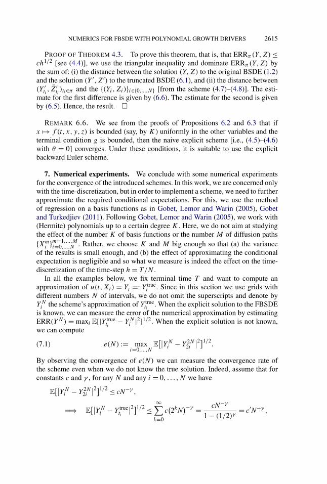
NUMERICS FOR FBSDE WITH POLYNOMIAL GROWTH DRIVERS 2615
PROOF OF THEOREM 4.3. To prove this theorem, that is, that ERRπ(Y,Z) ≤ch1/2 [see (4.4)], we use the triangular inequality and dominate ERRπ(Y,Z) bythe sum of: (i) the distance between the solution (Y,Z) to the original BSDE (1.2)and the solution (Y ′,Z′) to the truncated BSDE (6.1), and (ii) the distance between(Y ′
ti, Z′
ti)ti∈π and the {(Yi,Zi)}i∈{0,...,N} [from the scheme (4.7)–(4.8)]. The esti-
mate for the first difference is given by (6.6). The estimate for the second is givenby (6.5). Hence, the result. �
REMARK 6.6. We see from the proofs of Propositions 6.2 and 6.3 that ifx �→ f (t, x, y, z) is bounded (say, by K) uniformly in the other variables and theterminal condition g is bounded, then the naive explicit scheme [i.e., (4.5)–(4.6)with θ = 0] converges. Under these conditions, it is suitable to use the explicitbackward Euler scheme.
7. Numerical experiments. We conclude with some numerical experimentsfor the convergence of the introduced schemes. In this work, we are concerned onlywith the time-discretization, but in order to implement a scheme, we need to furtherapproximate the required conditional expectations. For this, we use the methodof regression on a basis functions as in Gobet, Lemor and Warin (2005), Gobetand Turkedjiev (2011). Following Gobet, Lemor and Warin (2005), we work with(Hermite) polynomials up to a certain degree K . Here, we do not aim at studyingthe effect of the number K of basis functions or the number M of diffusion paths{Xm
i }m=1,...,Mi=0,...,N . Rather, we choose K and M big enough so that (a) the variance
of the results is small enough, and (b) the effect of approximating the conditionalexpectation is negligible and so what we measure is indeed the effect on the time-discretization of the time-step h = T/N .
In all the examples below, we fix terminal time T and want to compute anapproximation of u(t,Xt) = Yt =: Y true
t . Since in this section we use grids withdifferent numbers N of intervals, we do not omit the superscripts and denote byYN
i the scheme’s approximation of Y trueti
. When the explicit solution to the FBSDEis known, we can measure the error of the numerical approximation by estimatingERR(YN) = maxi E[|Y true
ti− YN
i |2]1/2. When the explicit solution is not known,we can compute
e(N) := maxi=0,...,N
E[∣∣YN
i − Y 2N2i
∣∣2]1/2.(7.1)
By observing the convergence of e(N) we can measure the convergence rate ofthe scheme even when we do not know the true solution. Indeed, assume that forconstants c and γ , for any N and any i = 0, . . . ,N we have
E[∣∣YN
i − Y 2N2i
∣∣2]1/2 ≤ cN−γ ,
�⇒ E[∣∣YN
i − Y trueti
∣∣2]1/2 ≤∞∑
k=0
c(2kN
)−γ = cN−γ
1 − (1/2)γ= c′N−γ ,
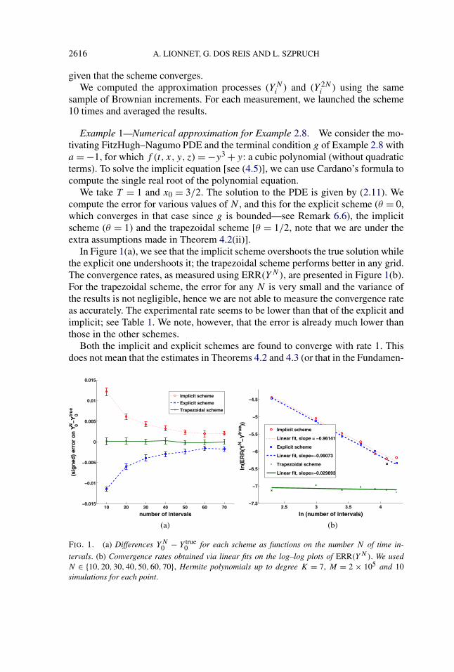
2616 A. LIONNET, G. DOS REIS AND L. SZPRUCH
given that the scheme converges.We computed the approximation processes (YN
i ) and (Y 2Ni ) using the same
sample of Brownian increments. For each measurement, we launched the scheme10 times and averaged the results.
Example 1—Numerical approximation for Example 2.8. We consider the mo-tivating FitzHugh–Nagumo PDE and the terminal condition g of Example 2.8 witha = −1, for which f (t, x, y, z) = −y3 + y: a cubic polynomial (without quadraticterms). To solve the implicit equation [see (4.5)], we can use Cardano’s formula tocompute the single real root of the polynomial equation.
We take T = 1 and x0 = 3/2. The solution to the PDE is given by (2.11). Wecompute the error for various values of N , and this for the explicit scheme (θ = 0,which converges in that case since g is bounded—see Remark 6.6), the implicitscheme (θ = 1) and the trapezoidal scheme [θ = 1/2, note that we are under theextra assumptions made in Theorem 4.2(ii)].
In Figure 1(a), we see that the implicit scheme overshoots the true solution whilethe explicit one undershoots it; the trapezoidal scheme performs better in any grid.The convergence rates, as measured using ERR(YN), are presented in Figure 1(b).For the trapezoidal scheme, the error for any N is very small and the variance ofthe results is not negligible, hence we are not able to measure the convergence rateas accurately. The experimental rate seems to be lower than that of the explicit andimplicit; see Table 1. We note, however, that the error is already much lower thanthose in the other schemes.
Both the implicit and explicit schemes are found to converge with rate 1. Thisdoes not mean that the estimates in Theorems 4.2 and 4.3 (or that in the Fundamen-
FIG. 1. (a) Differences YN0 − Y true
0 for each scheme as functions on the number N of time in-
tervals. (b) Convergence rates obtained via linear fits on the log–log plots of ERR(YN ). We usedN ∈ {10,20,30,40,50,60,70}, Hermite polynomials up to degree K = 7, M = 2 × 10⁵ and 10simulations for each point.
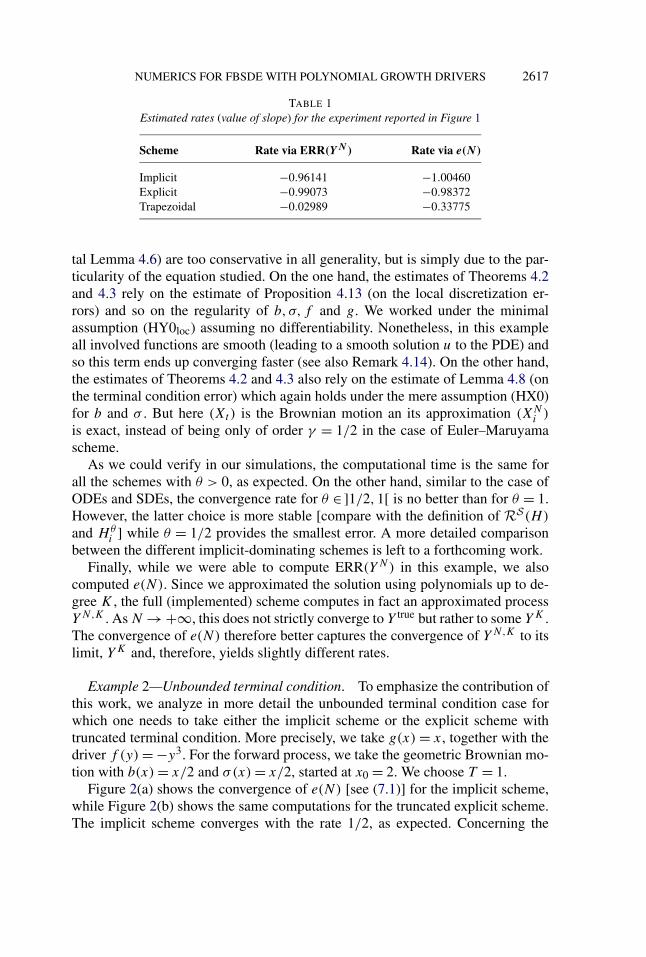
NUMERICS FOR FBSDE WITH POLYNOMIAL GROWTH DRIVERS 2617
TABLE 1Estimated rates (value of slope) for the experiment reported in Figure 1
Scheme Rate via ERR(YN) Rate via e(N)
Implicit −0.96141 −1.00460Explicit −0.99073 −0.98372Trapezoidal −0.02989 −0.33775
tal Lemma 4.6) are too conservative in all generality, but is simply due to the par-ticularity of the equation studied. On the one hand, the estimates of Theorems 4.2and 4.3 rely on the estimate of Proposition 4.13 (on the local discretization er-rors) and so on the regularity of b,σ,f and g. We worked under the minimalassumption (HY0loc) assuming no differentiability. Nonetheless, in this exampleall involved functions are smooth (leading to a smooth solution u to the PDE) andso this term ends up converging faster (see also Remark 4.14). On the other hand,the estimates of Theorems 4.2 and 4.3 also rely on the estimate of Lemma 4.8 (onthe terminal condition error) which again holds under the mere assumption (HX0)for b and σ . But here (Xt) is the Brownian motion an its approximation (XN
i )
is exact, instead of being only of order γ = 1/2 in the case of Euler–Maruyamascheme.
As we could verify in our simulations, the computational time is the same forall the schemes with θ > 0, as expected. On the other hand, similar to the case ofODEs and SDEs, the convergence rate for θ ∈]1/2,1[ is no better than for θ = 1.However, the latter choice is more stable [compare with the definition of RS(H)
and Hθi ] while θ = 1/2 provides the smallest error. A more detailed comparison
between the different implicit-dominating schemes is left to a forthcoming work.Finally, while we were able to compute ERR(YN) in this example, we also
computed e(N). Since we approximated the solution using polynomials up to de-gree K , the full (implemented) scheme computes in fact an approximated processYN,K . As N → +∞, this does not strictly converge to Y true but rather to some YK .The convergence of e(N) therefore better captures the convergence of YN,K to itslimit, YK and, therefore, yields slightly different rates.
Example 2—Unbounded terminal condition. To emphasize the contribution ofthis work, we analyze in more detail the unbounded terminal condition case forwhich one needs to take either the implicit scheme or the explicit scheme withtruncated terminal condition. More precisely, we take g(x) = x, together with thedriver f (y) = −y3. For the forward process, we take the geometric Brownian mo-tion with b(x) = x/2 and σ(x) = x/2, started at x0 = 2. We choose T = 1.
Figure 2(a) shows the convergence of e(N) [see (7.1)] for the implicit scheme,while Figure 2(b) shows the same computations for the truncated explicit scheme.The implicit scheme converges with the rate 1/2, as expected. Concerning the
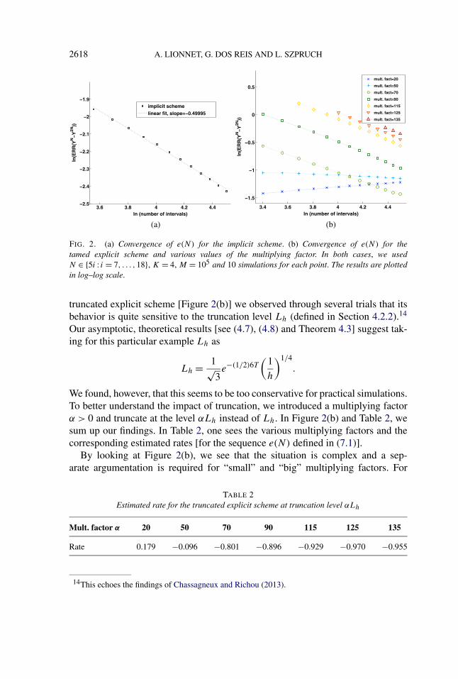
2618 A. LIONNET, G. DOS REIS AND L. SZPRUCH
FIG. 2. (a) Convergence of e(N) for the implicit scheme. (b) Convergence of e(N) for thetamed explicit scheme and various values of the multiplying factor. In both cases, we usedN ∈ {5i : i = 7, . . . ,18}, K = 4, M = 105 and 10 simulations for each point. The results are plottedin log–log scale.
truncated explicit scheme [Figure 2(b)] we observed through several trials that itsbehavior is quite sensitive to the truncation level Lh (defined in Section 4.2.2).14
Our asymptotic, theoretical results [see (4.7), (4.8) and Theorem 4.3] suggest tak-ing for this particular example Lh as
Lh = 1√3e−(1/2)6T
(1
h
)1/4
.
We found, however, that this seems to be too conservative for practical simulations.To better understand the impact of truncation, we introduced a multiplying factorα > 0 and truncate at the level αLh instead of Lh. In Figure 2(b) and Table 2, wesum up our findings. In Table 2, one sees the various multiplying factors and thecorresponding estimated rates [for the sequence e(N) defined in (7.1)].
By looking at Figure 2(b), we see that the situation is complex and a sep-arate argumentation is required for “small” and “big” multiplying factors. For
TABLE 2Estimated rate for the truncated explicit scheme at truncation level αLh
Mult. factor α 20 50 70 90 115 125 135
Rate 0.179 −0.096 −0.801 −0.896 −0.929 −0.970 −0.955
14This echoes the findings of Chassagneux and Richou (2013).
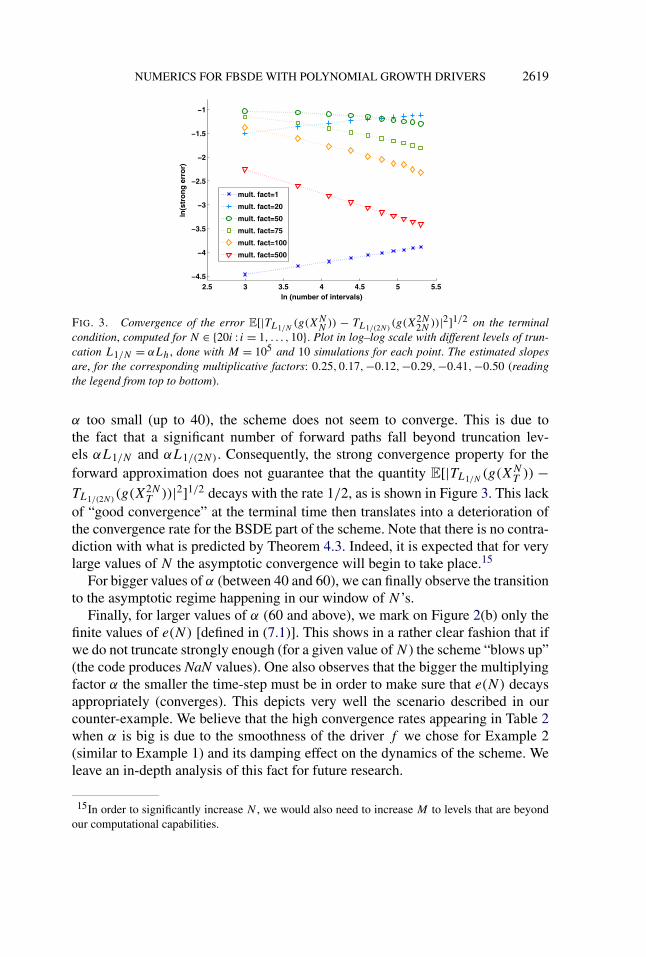
NUMERICS FOR FBSDE WITH POLYNOMIAL GROWTH DRIVERS 2619
FIG. 3. Convergence of the error E[|TL1/N(g(XN
N )) − TL1/(2N)(g(X2N
2N ))|2]1/2 on the terminalcondition, computed for N ∈ {20i : i = 1, . . . ,10}. Plot in log–log scale with different levels of trun-cation L1/N = αLh, done with M = 105 and 10 simulations for each point. The estimated slopesare, for the corresponding multiplicative factors: 0.25,0.17,−0.12,−0.29,−0.41,−0.50 (readingthe legend from top to bottom).
α too small (up to 40), the scheme does not seem to converge. This is due tothe fact that a significant number of forward paths fall beyond truncation lev-els αL1/N and αL1/(2N). Consequently, the strong convergence property for theforward approximation does not guarantee that the quantity E[|TL1/N
(g(XNT )) −
TL1/(2N)(g(X2N
T ))|2]1/2 decays with the rate 1/2, as is shown in Figure 3. This lackof “good convergence” at the terminal time then translates into a deterioration ofthe convergence rate for the BSDE part of the scheme. Note that there is no contra-diction with what is predicted by Theorem 4.3. Indeed, it is expected that for verylarge values of N the asymptotic convergence will begin to take place.15
For bigger values of α (between 40 and 60), we can finally observe the transitionto the asymptotic regime happening in our window of N ’s.
Finally, for larger values of α (60 and above), we mark on Figure 2(b) only thefinite values of e(N) [defined in (7.1)]. This shows in a rather clear fashion that ifwe do not truncate strongly enough (for a given value of N ) the scheme “blows up”(the code produces NaN values). One also observes that the bigger the multiplyingfactor α the smaller the time-step must be in order to make sure that e(N) decaysappropriately (converges). This depicts very well the scenario described in ourcounter-example. We believe that the high convergence rates appearing in Table 2when α is big is due to the smoothness of the driver f we chose for Example 2(similar to Example 1) and its damping effect on the dynamics of the scheme. Weleave an in-depth analysis of this fact for future research.
15In order to significantly increase N , we would also need to increase M to levels that are beyondour computational capabilities.
2620 A. LIONNET, G. DOS REIS AND L. SZPRUCH
APPENDIX
A.1. Motivating example. Before we state the main result, we recall a re-sult on the behavior of Gaussian random variables [which we do not prove, butthe reader is invited to try, in any case see Lemma 4.1 in Hutzenthaler, Jentzenand Kloeden (2011)]. The notation and probability spaces we work with in thisAppendix are as stated in Section 2.
LEMMA A.1. Let (�,F,P) be a probability space and let Z :� → R be anF/B(R)-measurable mapping with standard normal distribution. Then for anyx ∈ [0,∞) it holds that
P[|Z| ≥ x
]≥ 14xe−x2
.
The statement of Lemma 1.1 follows from the next lemma.
LEMMA A.2. Let πN denote the uniform grid of the time interval [0,1] withN +1 points and step size h := 1/N , where N ∈ N. Define the driver f (y) := −y3
and the terminal condition ξ ∈ Lp(F1) for any p ≥ 2. Let (Y,Z) be the uniquesolution to (1.3). Denote by {Y (N)
i }i∈{0,...,N} the Euler approximation of (Yt )t∈[0,1]defined via (1.4) over the grid πN .
Assume that N is fixed and that ξ verifies |ξ | ≥ 2√
N P-a.s. then:
(i) For any i ∈ {0, . . . ,N} it holds that |Yi | ≥ 22N−i√N .
Assume now that N is an even number (hence t = 1/2 is common to all gridsπN ) and denote by Y
(N)1/2 the approximation at the time point t = 1/2 (correspond-
ing to i = N/2). Define ξ as ξ := W1/2 ∈ Lp(F1) \ L∞(F1) for any p ≥ 1.
(ii) For any i ∈ {N2 , . . . ,N}, on the set {ω : ξ(ω) ≥ 2
√N} it holds that
|Yi(ω)| ≥ 22N−i√N .
(iii) Moreover, limN→∞E[|Y (N)1/2 |] = +∞.
PROOF. For the given f and ξ , the results from Section 2 in Pardoux (1999)combined with the a priori estimates stated in our Section 2 ensure the existenceand uniqueness of a solution (Y,Z) ∈ Sp ×Hp to BSDE (1.3) for any p ≥ 2. Wenow fix N and drop the superscript (N) from Y (N).
Proof of Part (i). Without loss of generality, assume that ξ = YN ≥ 2√
N . Then
YN−1 = EN−1[YN − Y 3
Nh]= EN−1
[YN
(1 − Y 2
Nh)]
.
Observe that Y 2N ≥ 2N which implies (1 − Y 2
Nh) ≤ (1 − 22) < 0. Hence (sinceYN > 0),
YN−1 = Ei
[YN
(1 − Y 2
Nh)]≤ −2
√N(22 − 1
)≤ −22√
N.

NUMERICS FOR FBSDE WITH POLYNOMIAL GROWTH DRIVERS 2621
Next (since YN−1 < 0) Y 2N−1 ≥ 24N which implies 1 − Y 2
N−1h ≤ (1 − 24) < 0.Hence,
YN−2 = Ei
[YN−1
(1 − Y 2
N−1h)]= Ei
[(−YN−1)
(Y 2
N−1h − 1)]
≥ 22√
N(24 − 1
)≥ 222√N.
Proceeding by induction, we can show that
|Yi | ≥ 22N−i√N.
Indeed, assume |Yi+1| ≥ 22N−i−1√N (in the light of above calculations; the nega-
tive case is analogous), then
Yi = Ei
[YN
(1 − Y 2
Nh)]≤ 22N−i−1√
N((
22N−i−1)2 − 1)≤ 22N−i√
N
and statement (i) is proved.Before proving (ii) and (iii), we remark that no conditional expectation needs
to be computed for the scheme (1.4) for i ∈ {N/2, . . . ,N} because ξ = W1/2 is
Ft -adapted for any t ∈ [1/2,1]. The scheme’s approximations up to Y(N)1/2 can be
written as
Y(N)N = W1/2, Y
(N)N−1 = ψ(W1/2),
Y(N)N−2 = ψ
(ψ(W1/2)
), . . . , Y
(N)N/2 = ψ◦(N/2)(W1/2),
where ψ(x) := x−hx3 and ψ◦(n) denotes the composition of ψ with itself n-times(n ∈ N).
Proof of Part (ii). We work on the event that ξ = YN ≥ 2√
N . We have first
YN−1 = EN−1[YN − Y 3
Nh]= YN
(1 − Y 2
Nh).
Observe that Y 2N ≥ 22N which implies (1 − Y 2
Nh) ≤ (1 − 22) < 0. Hence (sinceYN > 0),
YN−1 = YN
(1 − Y 2
Nh)≤ −2
√N(22 − 1
)≤ −22√
N < 0.
Next, since YN−1 < 0, Y 2N−1 ≥ 24N which implies 1 − Y 2
N−1h ≤ (1 − 24) < 0.Hence,
YN−2 = YN−1(1 − Y 2
N−1h)= −YN−1
(Y 2
N−1h − 1)≥ 22
√N(24 − 1
)≥ 222√N.
Proceeding by induction we can easily show that
|Yi | ≥ 22N−i√N, i = N
2, . . . ,N.
Indeed, assume Yi+1 ≥ 22N−i−1√N (note that in the light of the above calculations
the negative case is analogous). Then
Yi = Yi+1(1 − Y 2
i+1h)≤ 22N−i−1√
N(1 − (
22N−i−1)2)≤ −22N−i√N.
2622 A. LIONNET, G. DOS REIS AND L. SZPRUCH
Proof of Part (iii). It follows easily from Lemma A.1 that
P[|W1/2| ≥ 2
√N]≥ √
2
2
√Ne−8N.
Then, using part (i) (to go from the first to the second line) and the above remark(on the third line), we have
limN→∞E
[∣∣Y (N)1/2
∣∣]= lim
N→∞E[1{ξ≥2
√N}∣∣Y (N)
1/2
∣∣+ 1{ξ<2√
N}∣∣Y (N)
1/2
∣∣]≥ lim
N→∞E[1{ξ≥2
√N}∣∣Y (N)
1/2
∣∣]≥ lim
N→∞E[1{ξ≥2
√N}2
2N−N/2√N]
= limN→∞ 22N/2√
NP[|W1/2| ≥ 2
√N]
≥ limN→∞ 2(2N/2)
√2
2Ne−8N = +∞. �
A.2. Basics of Malliavin’s calculus. We briefly introduce the main notationof the stochastic calculus of variations also known as Malliavin’s calculus. Formore details, we refer the reader to Nualart (2006), for its application to BSDEswe refer to Imkeller (2008). Let S be the space of random variables of the form
ξ = F
((∫ T
0h1,i
s dW 1s
)1≤i≤n
, . . . ,
(∫ T
0hd,i
s dWds
)1≤i≤n
),
where F ∈ C∞b (Rn×d), h1, . . . , hn ∈ L2([0, T ];Rd), n ∈ N. To simplify nota-
tion, assume that all hj are written as row vectors. For ξ ∈ S , we define D =(D1, . . . ,Dd) :S → L2(� × [0, T ])d by
Diθξ =
n∑j=1
∂F
∂xi,j
(∫ T
0h1
t dWt, . . . ,
∫ T
0hn
t dWt
)h
i,jθ , 0 ≤ θ ≤ T ,1 ≤ i ≤ d,
and for k ∈ N its k-fold iteration by D(k) = (Di1 · · ·Dik )1≤i1,...,ik≤d . For k ∈ N,p ≥ 1 let Dk,p be the closure of S with respect to the norm
‖ξ‖pk,p = E
[‖ξ‖p
Lp +k∑
i=1
∥∥∣∣D(k)ξ∣∣∥∥p
(Hp)i
].
D(k) is a closed linear operator on the space Dk,p . Observe that if ξ ∈ D
1,2 isFt -measurable then Dθξ = 0 for θ ∈ (t, T ]. Further denote D
k,∞ =⋂p>1 D
k,p .We also need Malliavin’s calculus for Rm valued smooth stochastic processes.
For k ∈ N,p ≥ 1, denote by Lk,p(Rm) the set of Rm-valued progressively measur-
able processes u = (u1, . . . , um) on [0, T ] × � such that:
NUMERICS FOR FBSDE WITH POLYNOMIAL GROWTH DRIVERS 2623
(i) For Lebesgue-a.a. t ∈ [0, T ], u(t, ·) ∈ (Dk,p)m;(ii) [0, T ]×� � (t,ω) �→ D(k)u(t,ω) ∈ (L2([0, T ]1+k))d×n admits a progres-
sively measurable version;(iii) ‖u‖p
k,p = ‖u‖pHp +∑k
i=1 ‖Diu‖p
(Hp)1+i < ∞.
Note that Jensen’s inequality gives16 for all p ≥ 2
E
[(∫ T
0
∫ T
0|DuXt |2 dudt
)p/2]≤ T p/2−1
∫ T
0‖DuX‖p
Hp du.(A.1)
We recall a result from Imkeller (2008) concerning the rule for the Malliavin dif-ferentiation of Itô integrals which is of use in applications of Malliavin’s calculusto stochastic analysis.
THEOREM A.3 [Theorem 2.3.4 in Imkeller (2008)]. Let (Xt)t∈[0,T ] ∈ H2 bean adapted process and define Mt := ∫ t
0 Xr dWr for t ∈ [0, T ]. Then X ∈ L1,2 if
and only if Mt ∈ D1,2 for any t ∈ [0, T ].
Moreover, for any 0 ≤ s, t ≤ T we have
DsMt = Xs1{s≤t}(s) + 1{s≤t}(s)∫ t
sDsXr dWr.(A.2)
A.3. A particular Gronwall lemma. We state here a “discrete Gronwalllemma” of some kind, particularly useful for the numerical analysis of BSDEs,and which we use extensively in this work.
LEMMA A.4. Let ai , bi , ci , be such that ai, bi ≥ 0, ci ∈ R for i = 0,1, . . . ,N .Assume that, for some constant c > 0 and h > 0, we have
ai + bi ≤ (1 + ch)ai+1 + ci for i = 0,1, . . . ,N − 1.(A.3)
Then the following inequality holds for every i:
ai +N−1∑j=i
bj ≤ ec(N−i)haN +N−1∑j=i
ec(j−i)hcj .
PROOF. The estimate is clearly true for i = N − 1 (even for i = N in fact).Then, for any i ≤ N − 2, if it is true for i + 1, by multiplying both sides by ech wefind that
echai+1 + echN−1∑
j=i+1
bj ≤ ec(N−i)haN +N−1∑
j=i+1
ec(j−i)hcj .
Summing this inequality with (A.3) and noting that∑N−1
j=i+1 bj ≤ ech∑N−1j=i+1 bj
due to the positivity of the bj terms gives the sought estimate for any i. �
16The reason behind this last inequality is that within the BSDE framework the usual tools to obtaina priori estimates yield with much difficulty the LHS while with relative ease the RHS.
2624 A. LIONNET, G. DOS REIS AND L. SZPRUCH
Acknowledgments. We would like to thank Samuel Cohen (University of Ox-ford), Gechun Liang (King’s college) and Joscha Diehl (TU-Berlin) for helpfuldiscussions.
REFERENCES
ALANKO, S. and AVELLANEDA, M. (2013). Reducing variance in the numerical solution of BSDEs.C. R. Math. Acad. Sci. Paris 351 135–138. MR3038003
BOUCHARD, B. and TOUZI, N. (2004). Discrete-time approximation and Monte-Carlo simulation ofbackward stochastic differential equations. Stochastic Process. Appl. 111 175–206. MR2056536
BRIAND, P. and CARMONA, R. (2000). BSDEs with polynomial growth generators. J. Appl. Math.Stoch. Anal. 13 207–238. MR1782682
BRIAND, P. and CONFORTOLA, F. (2008). Differentiability of backward stochastic differential equa-tions in Hilbert spaces with monotone generators. Appl. Math. Optim. 57 149–176. MR2386102
BRIAND, PH., DELYON, B., HU, Y., PARDOUX, E. and STOICA, L. (2003). Lp solutions of back-ward stochastic differential equations. Stochastic Process. Appl. 108 109–129. MR2008603
CHASSAGNEUX, J. F. (2012). An introduction to the numerical approximation of BSDEs. Lecturenotes, 2nd Summer School of the Euro-Mediterranean Research Center for Mathematics and itsApplications (EMRCMA). Available at www.imperial.ac.uk/~jchassag/.
CHASSAGNEUX, J. F. (2013). Linear multi-step schemes for BSDEs. Preprint. Available atarXiv:1306.5548v1.
CHASSAGNEUX, J. F. and CRISAN, D. (2014). Runge–Kutta schemes for backward stochastic dif-ferential equations. Ann. Appl. Probab. 24 679–720. MR3178495
CHASSAGNEUX, J.-F. and RICHOU, A. (2013). Numerical simulation of quadratic BSDEs. Preprint.Available at arXiv:1307.5741.
CRISAN, D. and MANOLARAKIS, K. (2010). Second order discretization of backward SDEs andsimulation with the cubature method. Ann. Appl. Probab. 24 652–678. MR3178494
CRISAN, D. and MANOLARAKIS, K. (2012). Solving backward stochastic differential equationsusing the cubature method: Application to nonlinear pricing. SIAM J. Financial Math. 3 534–571. MR2968045
DOS REIS, G., RÉVEILLAC, A. and ZHANG, J. (2011). FBSDEs with time delayed generators:Lp-solutions, differentiability, representation formulas and path regularity. Stochastic Process.Appl. 121 2114–2150. MR2819244
EL KAROUI, N., PENG, S. and QUENEZ, M. C. (1997). Backward stochastic differential equationsin finance. Math. Finance 7 1–71. MR1434407
ESTEP, D. J., LARSON, M. G. and WILLIAMS, R. D. (2000). Estimating the error of numeri-cal solutions of systems of reaction–diffusion equations. Mem. Amer. Math. Soc. 146 viii+109.MR1692630
GOBET, E., LEMOR, J.-P. and WARIN, X. (2005). A regression-based Monte Carlo method to solvebackward stochastic differential equations. Ann. Appl. Probab. 15 2172–2202. MR2152657
GOBET, E. and TURKEDJIEV, P. (2011). Approximation of discrete BSDE using least-squares re-gression. Technical Report hal-00642685.
HENRY, D. (1981). Geometric Theory of Semilinear Parabolic Equations. Lecture Notes in Math.840. Springer, Berlin. MR0610244
HUTZENTHALER, M., JENTZEN, A. and KLOEDEN, P. E. (2011). Strong and weak divergencein finite time of Euler’s method for stochastic differential equations with non-globally Lips-chitz continuous coefficients. Proc. R. Soc. Lond. Ser. A Math. Phys. Eng. Sci. 467 1563–1576.MR2795791
HUTZENTHALER, M., JENTZEN, A. and KLOEDEN, P. E. (2012). Strong convergence of an ex-plicit numerical method for SDEs with nonglobally Lipschitz continuous coefficients. Ann. Appl.Probab. 22 1611–1641. MR2985171
NUMERICS FOR FBSDE WITH POLYNOMIAL GROWTH DRIVERS 2625
IMKELLER, P. (2008). Malliavin’s Calculus and Applications in Stochastic Control and Finance.IMPAN Lecture Notes 1. Polish Academy of Sciences, Institute of Mathematics, Warsaw.MR2494786
IMKELLER, P. and DOS REIS, G. (2010a). Path regularity and explicit convergence rate for BSDEwith truncated quadratic growth. Stochastic Process. Appl. 120 348–379. MR2584898
IMKELLER, P. and DOS REIS, G. (2010b). Corrigendum to “Path regularity and explicit convergencerate for BSDE with truncated quadratic growth” [Stochastic Process. Appl. 120 (2010) 348–379][MR2584898]. Stochastic Process. Appl. 120 2286–2288.
KLOEDEN, P. E. and PLATEN, E. (1992). Numerical Solution of Stochastic Differential Equations.Applications of Mathematics (New York) 23. Springer, Berlin. MR1214374
KOVÁCS, B. (2011). Semilinear parabolic problems. Master’s thesis, Eötvös Loránd Univ., Bu-dapest.
LIONNET, A. (2014). Topics on backward stochastic differential equations. Theoretical and practicalaspects. Ph.D. thesis, Oxford Univ.
MA, J. and ZHANG, J. (2002). Path regularity for solutions of backward stochastic differential equa-tions. Probab. Theory Related Fields 122 163–190. MR1894066
MAO, X. and SZPRUCH, L. (2013). Strong convergence rates for backward Euler–Maruyamamethod for non-linear dissipative-type stochastic differential equations with super-linear diffu-sion coefficients. Stochastics 85 144–171. MR3011916
MATOUSSI, A. and XU, M. (2008). Sobolev solution for semilinear PDE with obstacle under mono-tonicity condition. Electron. J. Probab. 13 1035–1067. MR2424986
MILSTEIN, G. N. and TRETYAKOV, M. V. (2004). Stochastic Numerics for Mathematical Physics.Scientific Computation. Springer, Berlin. MR2069903
NUALART, D. (2006). The Malliavin Calculus and Related Topics, 2nd ed. Springer, Berlin.MR2200233
PARDOUX, É. (1999). BSDEs, weak convergence and homogenization of semilinear PDEs. In Non-linear Analysis, Differential Equations and Control (Montreal, QC, 1998). NATO Sci. Ser. CMath. Phys. Sci. 528 503–549. Kluwer Academic, Dordrecht. MR1695013
ROTHE, F. (1984). Global Solutions of Reaction-Diffusion Systems. Lecture Notes in Math. 1072.Springer, Berlin. MR0755878
SÜLI, E. and MAYERS, D. F. (2003). An Introduction to Numerical Analysis. Cambridge Univ.Press, Cambridge. MR2006500
TOUZI, N. (2013). Optimal Stochastic Control, Stochastic Target Problems, and Backward SDE.Fields Institute Monographs 29. Springer, New York. MR2976505
ZEIDLER, E. (1990). Nonlinear Functional Analysis and Its Applications. II/B. Nonlinear MonotoneOperators. Springer, New York. Translated from the German by the author and Leo F. Boron.MR1033498
ZHANG, G., GUNZBURGER, M. and ZHAO, W. (2013). A sparse-grid method for multi-dimensionalbackward stochastic differential equations. J. Comput. Math. 31 221–248. MR3063734
ZHANG, Q. and ZHAO, H. (2012). Probabilistic representation of weak solutions of partial differen-tial equations with polynomial growth coefficients. J. Theoret. Probab. 25 396–423. MR2914434
A. LIONNET
OXFORD-MAN INSTITUTE
UNIVERSITY OF OXFORD
EAGLE HAUSE, WALTON WELL ROAD
OXFORD OX2 6EDUNITED KINGDOM
E-MAIL: [email protected]
G. DOS REIS
L. SZPRUCH
SCHOOL OF MATHEMATICS
UNIVERSITY OF EDINBURGH
EDINBURGH, EH9 3JZUNITED KINGDOM
E-MAIL: [email protected]@ed.ac.uk