chid, a x^2 -based discretization algorithm

ChiD, A -Based Discretization AlgorithmRoss Bettinger, Seattle, WA

ABSTRACT

We have developed a discretization algorithm, based on Kerber’s ChiMerge and Liu and Setiono’s Chi2, that automatically chooses the best set of cutpoints for dividing a continuous variable into a set of contiguous discrete intervals. The algorithm, ChiD, uses class information to perform supervised discretization based on maximizing the logworth of the significance of astatistic computed from adjacent intervals of the continuous variable being discretized. The ChiD algorithm generates cutpoints that match the quality of those computed by the Enterprise Miner Decision Tree algorithm as measured by the accuracy of classification models built using ChiD cutpoints versus original, undiscretized data.

KEYWORDSChi-squared, ChiMerge, Chi2, cutpoint, cutset, decision tree, discretization, SAS Enterprise Miner

INTRODUCTIONDiscretization of the many values of a continuous variable into a smaller number of disjoint, contiguous intervals is often a preprocessing step performed to reduce the number of distinct values, or states, that a variable may represent. For this purpose, discretization reduces model complexity and thereby provides insight into a model’s workings or may simplify the comparison between variables. Discretization may also be used for understanding a set of data by its effect of summarizing data into groups of similarity and difference, thus exposing patterns that reveal features of the data that would not otherwise be easily observed. Also, discretization provides appropriate inputs to classification algorithms that require discreteattributes for search, e.g., some decision tree algorithms and rule-based classifiers.Variables in data mining parlance are also called attributes because they represent attributes of a set of data under consideration. Both terms will be used in the following discussion.

of 14

TAXONOMY OF DISCRETIZATION ALGORITHMS1

Discretization algorithms may be classified according to their static/dynamic consideration of an attribute by itself or in relation to other attributes, and by their use of class information in the discretization process. In the case of static discretization, a single attribute by itself is considered, exclusive of any joint relationship with other attributes. In the case of dynamic discretization, all attributes are considered simultaneously with interdependencies among the attributes used in the computation of intervals. Discussion of dynamic discretization techniques is beyond the scope of this study. Algorithms that do not use class information are called unsupervised, while algorithms that do use class information are called supervised because thevariable’s class values provides “supervision”, or additional guidance, in theprocess of discretization.

UNSUPERVISED DISCRETIZATIONEqual-frequency discretization creates groups that ideally contain the same number of observations in each group. Data are first ranked and then collectedinto equally-sized groups (called quantiles) such as quartiles, quintiles, deciles, and percentiles. The width of each quantile may vary but the number of observations in each group is constant. If the data are not distributed as a multiple of the quantile, e.g., there are 99 or 101 observations for a percentile discretization, one or more groups will contain an observation lessor more than the specified number.Equal-width discretization is most frequently encountered in creating histograms whose class intervals are of fixed width, ideally based on domain knowledge but more often determined by convenience. For example, in financial reporting, dollar amounts are rounded to the nearest thousand (M), million (MM), billion (B), or trillion (T). Age ranges may be specified in 10-year groupings, e.g., 10-19, 20-29, 30-39, &c. The size of the interval may be based on past experience or intuition, but often not determined by objective, data-driven considerations. The SAS Enterprise Miner Transformation node bucketing algorithm, used in this study to create unsupervised discretized attributes, produces n class intervals of equal width. The class intervals usually contain unequal numbers of observations.Unsupervised discretization algorithms are straightforward to implement in code and produce results that are easy to understand. However, they generally do not contain as much information as supervised algorithms because they do not use a class attribute to “supervise” the discretization process.

1 Taxonomy adapted from [1].

of 14

SUPERVISED DISCRETIZATIONSupervised discretization algorithms use the additional information contained in a class variable, separate from the variable being discretized, to provide feedback to the discretization process. The class variable is typically the target variable in a modeling exercise. It contains data values, or class labels, representing behavior that is to be captured through the modeling process as a mathematical expression or as a set of rules. The class labels are categorical values used to compute some measure of optimality derived fromgrouping contiguous continuous values into intervals bounded by cutpoints. Theset of cutpoints is also called a cutset.One algorithm that uses the class labels as information is the Minimum Description Length Principle (MDLP) algorithm developed by Fayyad and Irani [2]. This algorithm uses class information entropy to select cutpoints of a continuous attribute that minimize the sum of the entropies of the class attribute on the intervals induced by the cutpoints. The algorithm’s tendency to produce an excess of cutpoints has been addressed by An and Cercone [3].

The focus of this study is another approach, ChiD, which uses thestatistic. It incorporates Kerber’s ChiMerge technique [4] and extends Liu andSetiono’s Chi2 algorithm [5]. The ChiMerge algorithm initially assigns each observation to its own interval, then uses the statistic to determine whether or not two adjacent intervals ought to be merged. If the significance of the statistic for the frequencies of the class values of the two intervals is greater than a specified , the intervals are merged. Otherwise,they remain distinct. Merging continues repetitively until no more pairs of intervals qualify for combining. ChiMerge requires that the significance level, , of the test be supplied as a parameter. You would have to manuallyexecute the algorithm with varying to produce useful results. Chi2 automatesthe ChiMerge algorithm by systematically varying through a range of values but it requires that the termination criterion, the maximum tolerable inconsistency2, be specified a priori. The ChiD algorithm described below automatically varies similarly to Chi2 and additionally determines the best cutset for a continuous variable as determined by maximizing the logworth of the test. It needs no a priori information.

CHID ALGORITHMThe ChiD algorithm uses the ChiMerge algorithm to compute a set of cutpoints for a specified significance level, . It incorporates Liu and Setiono’s 2 Inconsistency is related to the data mining concepts of heterogeneity or impurity and refers to the presence of multiple instances of distinct class labels in an interval of data. See [5] for more discussion.

of 14

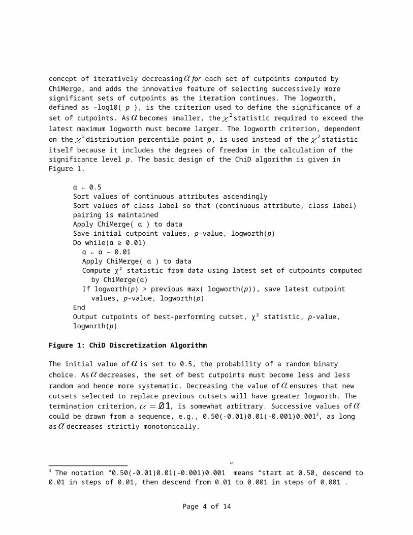
concept of iteratively decreasing for each set of cutpoints computed by ChiMerge, and adds the innovative feature of selecting successively more significant sets of cutpoints as the iteration continues. The logworth, defined as –log10( p ), is the criterion used to define the significance of a set of cutpoints. As becomes smaller, the statistic required to exceed thelatest maximum logworth must become larger. The logworth criterion, dependent on the distribution percentile point p, is used instead of the statistic itself because it includes the degrees of freedom in the calculation of the significance level p. The basic design of the ChiD algorithm is given in Figure 1.

α ← 0.5Sort values of continuous attributes ascendinglySort values of class label so that (continuous attribute, class label) pairing is maintainedApply ChiMerge( α ) to dataSave initial cutpoint values, p-value, logworth(p)Do while(α ≥ 0.01)

α ← α – 0.01Apply ChiMerge( α ) to dataCompute χ² statistic from data using latest set of cutpoints computed

by ChiMerge(α)If logworth(p) > previous max( logworth(p)), save latest cutpoint

values, p-value, logworth(p)EndOutput cutpoints of best-performing cutset, χ² statistic, p-value, logworth(p)

Figure 1: ChiD Discretization Algorithm

The initial value of is set to 0.5, the probability of a random binary choice. As decreases, the set of best cutpoints must become less and less random and hence more systematic. Decreasing the value of ensures that new cutsets selected to replace previous cutsets will have greater logworth. The termination criterion, , is somewhat arbitrary. Successive values ofcould be drawn from a sequence, e.g., 0.50(-0.01)0.01(-0.001)0.0013, as long as decreases strictly monotonically.

3 The notation “0.50(-0.01)0.01(-0.001)0.001” means “start at 0.50, descend to0.01 in steps of 0.01, then descend from 0.01 to 0.001 in steps of 0.001”.

of 14

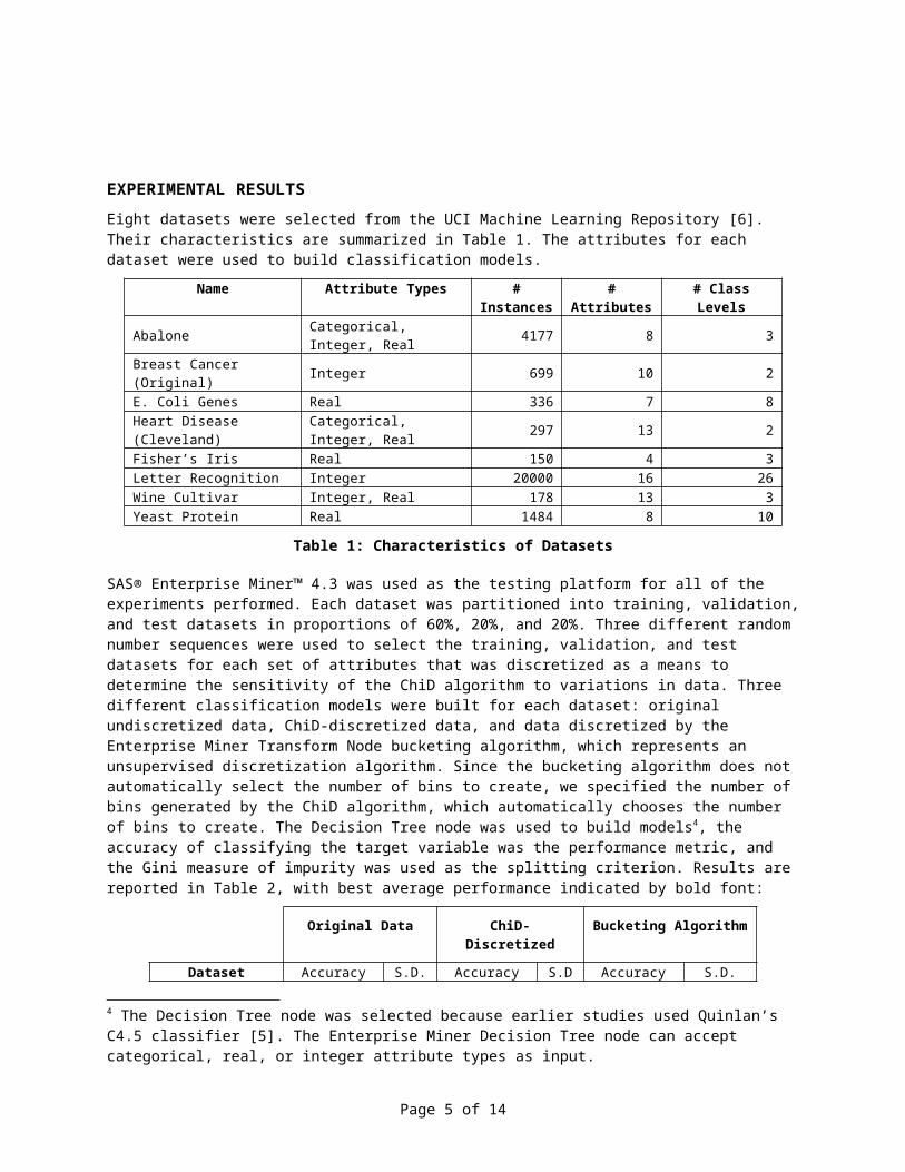
EXPERIMENTAL RESULTSEight datasets were selected from the UCI Machine Learning Repository [6]. Their characteristics are summarized in Table 1. The attributes for each dataset were used to build classification models.

Name Attribute Types #Instances

#Attributes

# ClassLevels

Abalone Categorical, Integer, Real 4177 8 3

Breast Cancer (Original) Integer 699 10 2

E. Coli Genes Real 336 7 8Heart Disease (Cleveland)

Categorical, Integer, Real 297 13 2

Fisher’s Iris Real 150 4 3Letter Recognition Integer 20000 16 26Wine Cultivar Integer, Real 178 13 3Yeast Protein Real 1484 8 10

Table 1: Characteristics of Datasets

SAS® Enterprise Miner™ 4.3 was used as the testing platform for all of the experiments performed. Each dataset was partitioned into training, validation,and test datasets in proportions of 60%, 20%, and 20%. Three different random number sequences were used to select the training, validation, and test datasets for each set of attributes that was discretized as a means to determine the sensitivity of the ChiD algorithm to variations in data. Three different classification models were built for each dataset: original undiscretized data, ChiD-discretized data, and data discretized by the Enterprise Miner Transform Node bucketing algorithm, which represents an unsupervised discretization algorithm. Since the bucketing algorithm does not automatically select the number of bins to create, we specified the number of bins generated by the ChiD algorithm, which automatically chooses the number of bins to create. The Decision Tree node was used to build models4, the accuracy of classifying the target variable was the performance metric, and the Gini measure of impurity was used as the splitting criterion. Results are reported in Table 2, with best average performance indicated by bold font:

Original Data ChiD-Discretized

Bucketing Algorithm

Dataset Accuracy S.D. Accuracy S.D Accuracy S.D.

4 The Decision Tree node was selected because earlier studies used Quinlan’s C4.5 classifier [5]. The Enterprise Miner Decision Tree node can accept categorical, real, or integer attribute types as input.

of 14

(%) (%) . (%)

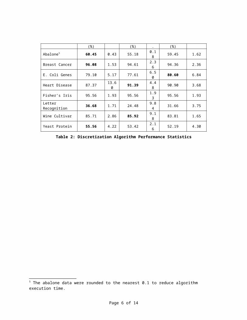
Abalone5 60.45 0.43 55.18 0.18 59.45 1.62

Breast Cancer 96.08 1.53 94.61 2.36 94.36 2.36

E. Coli Genes 79.10 5.17 77.61 6.50 80.60 6.84

Heart Disease 87.37 13.60 91.39 4.4

8 90.90 3.68

Fisher’s Iris 95.56 1.93 95.56 1.93 95.56 1.93

Letter Recognition 36.68 1.71 24.48 9.8

4 31.66 3.75

Wine Cultivar 85.71 2.86 85.92 9.18 83.81 1.65

Yeast Protein 55.56 4.22 53.42 2.16 52.19 4.30

Table 2: Discretization Algorithm Performance Statistics

5 The abalone data were rounded to the nearest 0.1 to reduce algorithm execution time.

of 14

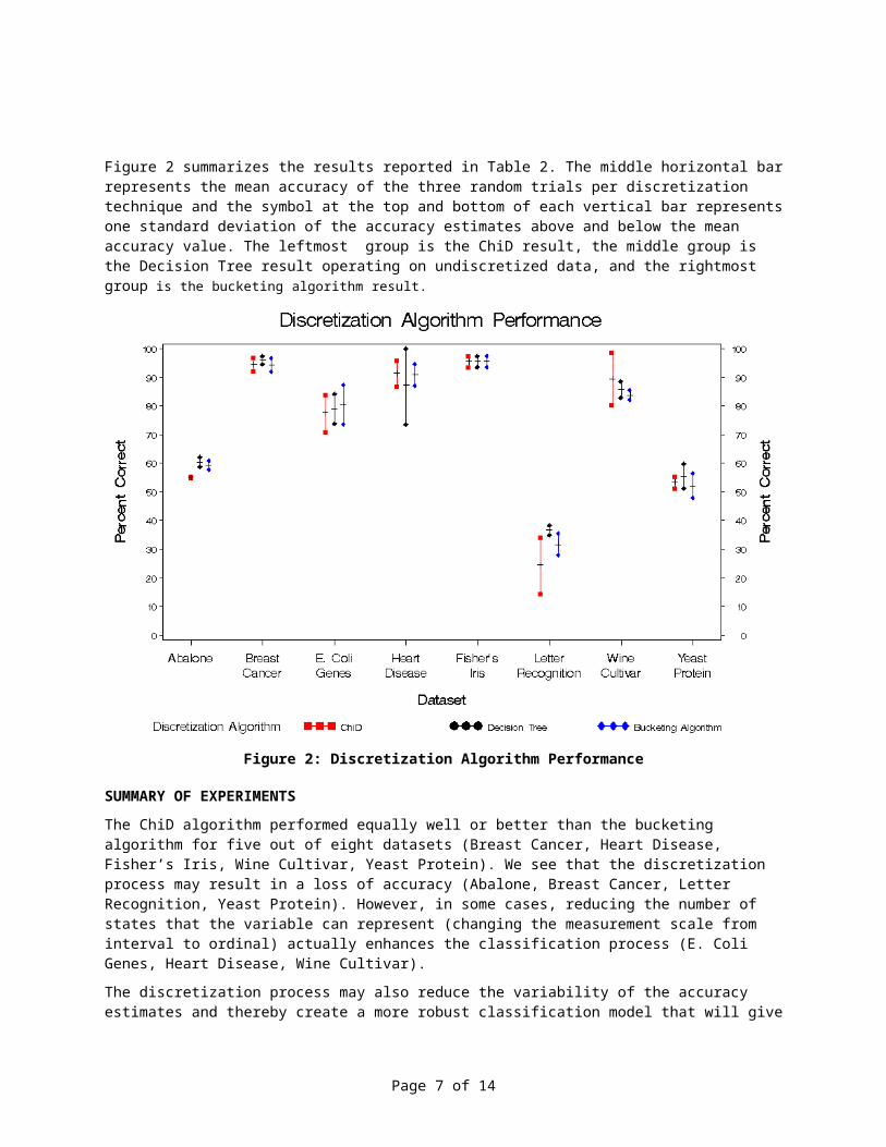
Figure 2 summarizes the results reported in Table 2. The middle horizontal barrepresents the mean accuracy of the three random trials per discretization technique and the symbol at the top and bottom of each vertical bar representsone standard deviation of the accuracy estimates above and below the mean accuracy value. The leftmost group is the ChiD result, the middle group is the Decision Tree result operating on undiscretized data, and the rightmost group is the bucketing algorithm result.

Figure 2: Discretization Algorithm Performance

SUMMARY OF EXPERIMENTSThe ChiD algorithm performed equally well or better than the bucketing algorithm for five out of eight datasets (Breast Cancer, Heart Disease, Fisher’s Iris, Wine Cultivar, Yeast Protein). We see that the discretization process may result in a loss of accuracy (Abalone, Breast Cancer, Letter Recognition, Yeast Protein). However, in some cases, reducing the number of states that the variable can represent (changing the measurement scale from interval to ordinal) actually enhances the classification process (E. Coli Genes, Heart Disease, Wine Cultivar).The discretization process may also reduce the variability of the accuracy estimates and thereby create a more robust classification model that will give

of 14

reliable classification decisions when new data are processed through a model that includes discretized attributes.

SENSITIVITY TO DATAAn important factor in the experimental design was the application of the “treatments”, e.g., discretization using the Decision Tree algorithm on original data, ChiD discretization, and unsupervised bucketing algorithm discretization, to random samples of each original dataset. This action was performed to investigate the sensitivity of each algorithm to fluctuations in the data used to construct each cutset, because data fluctuations are to be expected in an uncontrolled environment. We used Fisher’s iris data to illustrate sample-dependent sensitivity to discretization.

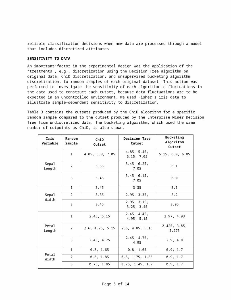
Table 3 contains the cutsets produced by the ChiD algorithm for a specific random sample compared to the cutset produced by the Enterprise Miner DecisionTree from undiscretized data. The bucketing algorithm, which used the same number of cutpoints as ChiD, is also shown.

IrisVariable

RandomSample

ChiDCutset

Decision TreeCutset

BucketingAlgorithmCutset

SepalLength

1 4.85, 5.9, 7.05 4.85, 5.45,6.15, 7.05 5.15, 6.0, 6.85

2 5.55 5.45, 6.25,7.05 6.1

3 5.45 5.45, 6.15,7.05 6.0

SepalWidth

1 3.45 3.35 3.1

2 3.35 2.95, 3.35, 3.2

3 3.45 2.95, 3.15,3.25, 3.45 3.05

PetalLength

1 2.45, 5.15 2.45, 4.45,4.95, 5.15 2.97, 4.93

2 2.6, 4.75, 5.15 2.6, 4.85, 5.15 2.425, 3.85,5.275

3 2.45, 4.75 2.45, 4.75,4.95 2.9, 4.8

PetalWidth

1 0.8, 1.65 0.8, 1.65 0.9, 1.7

2 0.8, 1.85 0.8, 1.75, 1.85 0.9, 1.7

3 0.75, 1.85 0.75, 1.45, 1.7 0.9, 1.7

of 14

Table 3: Sensitivity to Discretization

of 14

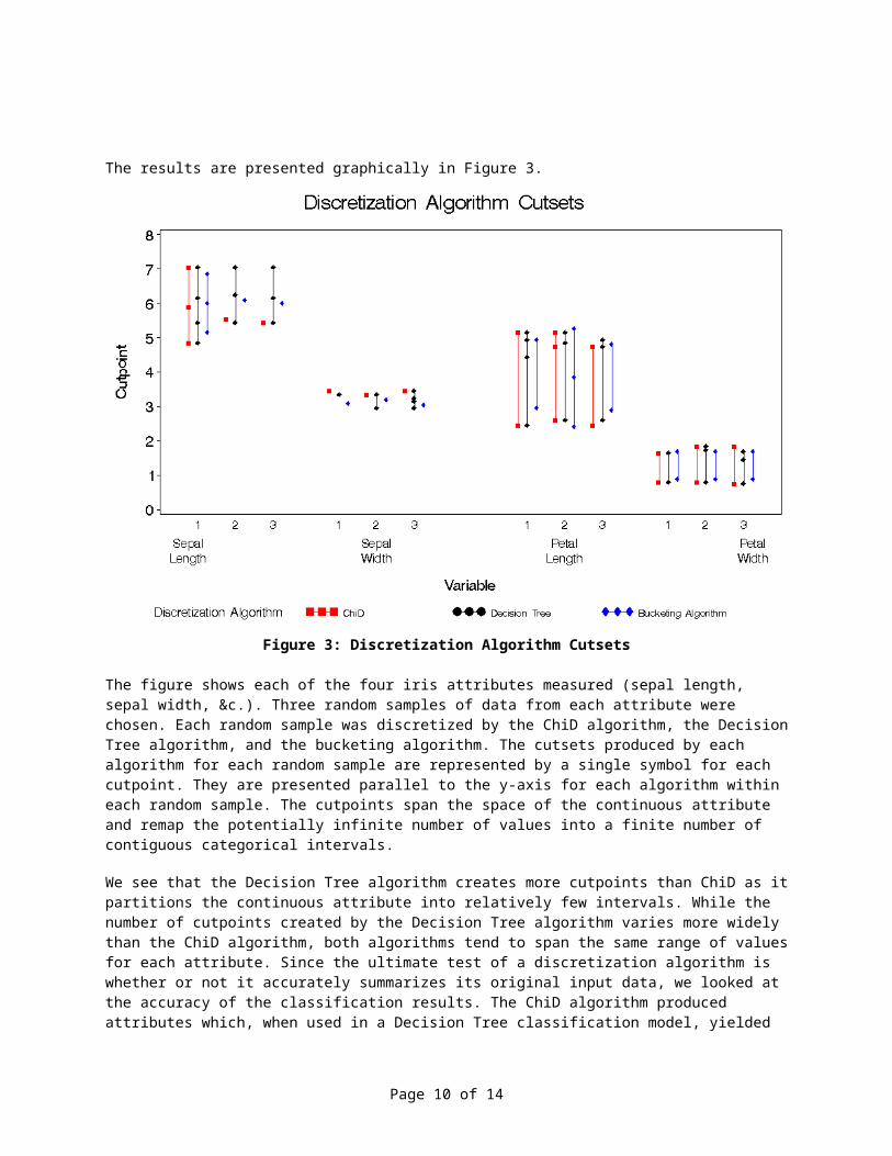
The results are presented graphically in Figure 3.

Figure 3: Discretization Algorithm Cutsets

The figure shows each of the four iris attributes measured (sepal length, sepal width, &c.). Three random samples of data from each attribute were chosen. Each random sample was discretized by the ChiD algorithm, the DecisionTree algorithm, and the bucketing algorithm. The cutsets produced by each algorithm for each random sample are represented by a single symbol for each cutpoint. They are presented parallel to the y-axis for each algorithm within each random sample. The cutpoints span the space of the continuous attribute and remap the potentially infinite number of values into a finite number of contiguous categorical intervals.

We see that the Decision Tree algorithm creates more cutpoints than ChiD as itpartitions the continuous attribute into relatively few intervals. While the number of cutpoints created by the Decision Tree algorithm varies more widely than the ChiD algorithm, both algorithms tend to span the same range of valuesfor each attribute. Since the ultimate test of a discretization algorithm is whether or not it accurately summarizes its original input data, we looked at the accuracy of the classification results. The ChiD algorithm produced attributes which, when used in a Decision Tree classification model, yielded

of 14

average results that were within one standard deviation of the Decision Tree algorithm results for six out of the eight datasets used in this study (BreastCancer, E.Coli Genes, Heart Disease, Fisher’s Iris, Wine Cultivars, and Yeast Protein). It appears that the ChiD algorithm creates similar cutsets as the Decision Tree algorithm.

CONCLUSIONWe have developed a -based discretization algorithm, ChiD, based on previous work [4, 5] that automatically produces a set of cutpoints over the values of a continuous variable using class information contained in a categorical variable. We tested the algorithm using datasets representing a variety of knowledge domains from [6]. We observed that the ChiD algorithm generates cutsets that are of similar quality to those computed by the Enterprise Miner Decision Tree algorithm in that classification models that used them to summarize dataset attributes are reasonably as accurate as those produced by the Decision Tree algorithm operating on undiscretized data for six out of eight datasets.

of 14

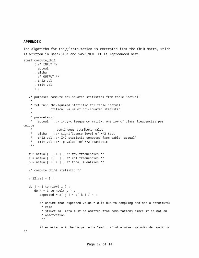
APPENDIXThe algorithm for the computation is excerpted from the ChiD macro, which is written in Base/SAS® and SAS/IML®. It is reproduced here.start compute_chi2 ( /* INPUT */ actual , alpha /* OUTPUT */ , chi2_val , crit_val ) ;

/* purpose: compute chi-squared statistics from table 'actual' * * returns: chi-squared statistic for table 'actual', * critical value of chi-squared statistic * * parameters: * actual ::= r-by-c frequency matrix: one row of class frequencies per unique * continuous attribute value * alpha ::= significance level of X^2 test * chi2_val ::= X^2 statistic computed from table ‘actual’ * crit_val ::= ‘p-value’ of X^2 statistic */

r = actual[ , + ] ; /* row frequencies */ c = actual[ +, ] ; /* col frequencies */ n = actual[ +, + ] ; /* total # entries */

/* compute chi^2 statistic */

chi2_val = 0 ;

do j = 1 to nrow( r ) ; do k = 1 to ncol( c ) ; expected = r[ j ] * c[ k ] / n ;

/* assume that expected value = 0 is due to sampling and not a structural * zero * structural zero must be omitted from computations since it is not an * observation */

if expected = 0 then expected = 1e-6 ; /* otherwise, zerodivide condition */

of 14

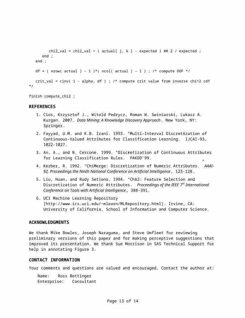
chi2_val = chi2_val + ( actual[ j, k ] - expected ) ## 2 / expected ; end ; end ;

df = ( nrow( actual ) - 1 )*( ncol( actual ) - 1 ) ; /* compute DOF */

crit_val = cinv( 1 - alpha, df ) ; /* compute crit value from inverse chi^2 cdf */

finish compute_chi2 ;

REFERENCES1. Cios, Krzysztof J., Witold Pedrycz, Roman W. Swiniarski, Lukasz A.

Kurgan. 2007. Data Mining: A Knowledge Discovery Approach. New York, NY: Springer.

2. Fayyad, U.M. and K.B. Irani. 1993. “Multi-Interval Discretization of Continuous-Valued Attributes for Classification Learning.” IJCAI-93, 1022-1027.

3. An, A., and N. Cercone. 1999. “Discretization of Continuous Attributes for Learning Classification Rules.” PAKDD’99.

4. Kerber, R. 1992. “ChiMerge: Discretization of Numeric Attributes.” AAAI-92, Proceedings the Ninth National Conference on Artificial Intelligence, 123-128.

5. Liu, Huan, and Rudy Setiono. 1994. “Chi2: Feature Selection and Discretization of Numeric Attributes.” Proceedings of the IEEE 7th International Conference on Tools with Artificial Intelligence, 388-391.

6. UCI Machine Learning Repository [http://www.ics.uci.edu/~mlearn/MLRepository.html]. Irvine, CA: University of California, School of Information and Computer Science.

ACKNOWLEDGMENTS

We thank Mike Bowles, Joseph Naraguma, and Steve Umfleet for reviewing preliminary versions of this paper and for making perceptive suggestions that improved its presentation. We thank Sue Morrison in SAS Technical Support for help in annotating Figure 3.

CONTACT INFORMATIONYour comments and questions are valued and encouraged. Contact the author at:

Name: Ross BettingerEnterprise: Consultant

of 14

E-mail: [email protected]

SAS and all other SAS Institute Inc. product or service names are registered trademarks or trademarks of SAS Institute Inc. in the USA and other countries.® indicates USA registration. Other brand and product names are trademarks of their respective companies.

of 14

chid, a x^2 -based discretization algorithm

Documents