adaptive discretization for episodic reinforcement learning
TRANSCRIPT
55
Adaptive Discretization for Episodic Reinforcement
Learning in Metric Spaces
SEAN R. SINCLAIR, Cornell University, USA
SIDDHARTHA BANERJEE, Cornell University, USA
CHRISTINA LEE YU, Cornell University, USA
We present an ecient algorithm for model-free episodic reinforcement learning on large (potentially con-
tinuous) state-action spaces. Our algorithm is based on a novel Q-learning policy with adaptive data-driven
discretization. The central idea is to maintain a ner partition of the state-action space in regions which
are frequently visited in historical trajectories, and have higher payo estimates. We demonstrate how our
adaptive partitions take advantage of the shape of the optimal Q-function and the joint space, without sac-
ricing the worst-case performance. In particular, we recover the regret guarantees of prior algorithms for
continuous state-action spaces, which additionally require either an optimal discretization as input, and/or
access to a simulation oracle. Moreover, experiments demonstrate how our algorithm automatically adapts to
the underlying structure of the problem, resulting in much better performance compared both to heuristics
and Q-learning with uniform discretization.
CCS Concepts: • Computing methodologies→ Q-learning; Sequential decision making; Continuous space
search; • Theory of computation → Markov decision processes;
Keywords: reinforcement learning, metric spaces, adaptive discretization, Q-learning, model-free
ACM Reference Format:
Sean R. Sinclair, Siddhartha Banerjee, and Christina Lee Yu. 2019. Adaptive Discretization for Episodic
Reinforcement Learning in Metric Spaces. In Proc. ACM Meas. Anal. Comput. Syst., Vol. 3, 3, Article 55
(December 2019). ACM, New York, NY. 44 pages. https://doi.org/10.1145/3366703
1 INTRODUCTION
Reinforcement learning (RL) is a natural model for systems involving real-time sequential decisionmaking [26]. An agent interacts with a system having stochastic transitions and rewards, and aimsto learn to control the system by exploring available actions and using real-time feedback. Thisrequires the agent to navigate the exploration exploitation trade-o, between exploring unseen partsof the environment and exploiting historical high-reward actions. In addition, many RL problemsinvolve large state-action spaces, which makes learning and storing the entire transition kernelinfeasible (for example, in memory-constrained devices). This motivates the use of model-free
RL algorithms, which eschew learning transitions and focus only on learning good state-actionmappings. The most popular of these algorithms is Q-learning [2, 10, 29], which forms the focus ofour work.
The code for the experiments is available at https://github.com/seanrsinclair/AdaptiveQLearning.
Authors’ addresses: Sean R. Sinclair, [email protected], Cornell University, USA; Siddhartha Banerjee, sbanerjee@cornell.
edu, Cornell University, USA; Christina Lee Yu, [email protected], Cornell University, USA.
Permission to make digital or hard copies of all or part of this work for personal or classroom use is granted without fee
provided that copies are not made or distributed for prot or commercial advantage and that copies bear this notice and the
full citation on the rst page. Copyrights for components of this work owned by others than the author(s) must be honored.
Abstracting with credit is permitted. To copy otherwise, or republish, to post on servers or to redistribute to lists, requires
prior specic permission and/or a fee. Request permissions from [email protected].
© 2019 Copyright held by the owner/author(s). Publication rights licensed to ACM.
2476-1249/2019/12-ART55 $15.00
https://doi.org/10.1145/3366703
Proc. ACM Meas. Anal. Comput. Syst., Vol. 3, No. 3, Article 55. Publication date: December 2019.
55:2 Sean R. Sinclair, Siddhartha Banerjee, and Christina Lee Yu
In even higher-dimensional state-spaces, in particular, continuous spaces, RL algorithms requireembedding the setting in some metric space, and then using an appropriate discretization ofthe space. A major challenge here is in learning an “optimal” discretization, trading-o memoryrequirements and algorithm performance. Moreover, unlike optimal quantization problems in‘oine’ settings (i.e., where the full problem is specied), there is an additional challenge of learninga good discretization and control policy when the process of learning itself must also be constrainedto the available memory. This motivates our central question:
Can we modify Q-learning to learn a near-optimal policy while limiting the size of the discretization?
Current approaches to this problem consider uniform discretization policies, which are eitherxed based on problem primitives, or updated via a xed schedule (for example, via a ‘doublingtrick’). However, a more natural approach is to adapt the discretization over space and time in adata-driven manner. This allows the algorithm to learn policies which are not uniformly smooth,but adapt to the geometry of the underlying space. Moreover, the agent would then be able toexplore more eciently by only sampling important regions.Adaptive discretization has been proposed and studied in the simpler multi-armed bandit set-
tings [12, 23]. The key idea here is to develop a non-uniform partitioning of the space, whosecoarseness depends on the density of past observations. These techniques, however, do not immedi-ately extend to RL, with the major challenge being in dealing with error propagation over periods.In more detail, in bandit settings, an algorithm’s regret (i.e., additive loss from the optimal policy)can be decomposed in straightforward ways, so as to isolate errors and control their propagation.Since errors can propagate in complex ways over sample paths, naive discretization could result inover-partitioning suboptimal regions of the space (leading to over exploration), or not discretizingenough in the optimal region due to noisy samples (leading to loss in exploitation). Our work takesan important step towards tackling these issues.Adaptive partitioning for reinforcement learning makes progress towards addressing the chal-
lenge of limited memory for real-time control problems. In particular, we are motivated by con-sidering the use of RL for computing systems problems such as memory management, resourceallocation, and load balancing [6, 15]. These are applications in which the process of learning theoptimal control policy must be implemented directly on-chip due to latency constraints, leadingto restrictive memory constraints. Adaptive partitioning nds a more “ecient” discretization ofthe space for the problem instance at hand, reducing the memory requirements. This could haveuseful applications to many control problems, even with discrete state spaces, as long as the modelexhibits “smoothness” structure between nearby state-action pairs.
1.1 Our Contributions
As the main contribution of this paper, we design and analyze a Q-learning algorithm based on
data-driven adaptive discretization of the state-action space. Our algorithm only requires that theunderlying state-action space can be embedded in a compact metric space, and that the optimalQ-function is Lipschitz continuous with respect to the metric. This setting is general, encompassingdiscrete and continuous state-action spaces, deterministic systems with natural metric structures,and stochastic settings with mild regularity assumptions on the transition kernels. Notably, ouralgorithm only requires access to the metric, unlike other algorithms which require access tosimulation oracles. In addition, our algorithm is model-free, requiring less space and computationalcomplexity to learn the optimal policy.From a theoretical perspective, we show that our adaptive discretization policy achieves near-
optimal dependence of the regret on the covering dimension of the metric space. In particular, we
Proc. ACM Meas. Anal. Comput. Syst., Vol. 3, No. 3, Article 55. Publication date: December 2019.
Adaptive Discretization for Episodic Reinforcement Learning in Metric Spaces 55:3
0 1000 2000 3000 4000 5000
Episode
0
1
2
3
4
5
ObservedReward
Comparison of Observed Rewards
Adaptive
Epsilon Net
0.0 0.2 0.4 0.6 0.8 1.0
State Space
0.0
0.2
0.4
0.6
0.8
1.0
ActionSpace
Uniform Discretization
0.0 0.2 0.4 0.6 0.8 1.0
State Space
0.0
0.2
0.4
0.6
0.8
1.0
ActionSpace
Adaptive Discretization
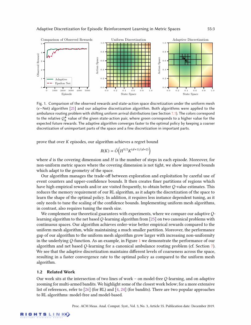
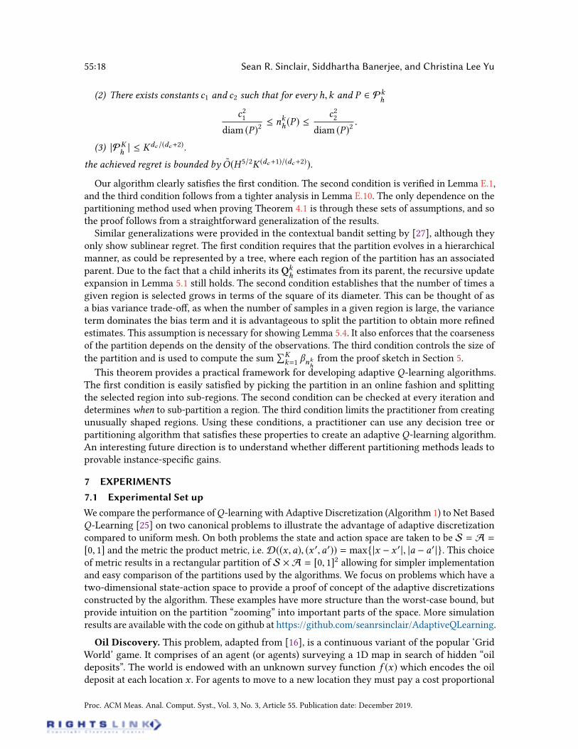
Fig. 1. Comparison of the observed rewards and state-action space discretization under the uniform mesh
(Net) algorithm [25] and our adaptive discretization algorithm. Both algorithms were applied to the
ambulance routing problem with shiing uniform arrival distributions (see Section 7.1). The colors correspond
to the relative Q?
hvalue of the given state-action pair, where green corresponds to a higher value for the
expected future rewards. The adaptive algorithm converges faster to the optimal policy by keeping a coarser
discretization of unimportant parts of the space and a fine discretization in important parts.
prove that over K episodes, our algorithm achieves a regret bound
R(K) = OH 5/2K (d+1)/(d+2)
where d is the covering dimension and H is the number of steps in each episode. Moreover, fornon-uniform metric spaces where the covering dimension is not tight, we show improved boundswhich adapt to the geometry of the space.
Our algorithm manages the trade-o between exploration and exploitation by careful use ofevent counters and upper-condence bounds. It then creates ner partitions of regions whichhave high empirical rewards and/or are visited frequently, to obtain better Q-value estimates. Thisreduces the memory requirement of our RL algorithm, as it adapts the discretization of the space tolearn the shape of the optimal policy. In addition, it requires less instance dependent tuning, as itonly needs to tune the scaling of the condence bounds. Implementing uniform mesh algorithms,in contrast, also requires tuning the mesh size.
We complement our theoretical guarantees with experiments, where we compare our adaptiveQ-learning algorithm to the net basedQ-learning algorithm from [25] on two canonical problems withcontinuous spaces. Our algorithm achieves order-wise better empirical rewards compared to theuniform mesh algorithm, while maintaining a much smaller partition. Moreover, the performancegap of our algorithm to the uniform mesh algorithm grow larger with increasing non-uniformityin the underlying Q-function. As an example, in Figure 1 we demonstrate the performance of ouralgorithm and net based Q-learning for a canonical ambulance routing problem (cf. Section 7).We see that the adaptive discretization maintains dierent levels of coarseness across the space,resulting in a faster convergence rate to the optimal policy as compared to the uniform meshalgorithm.
1.2 Related Work
Our work sits at the intersection of two lines of work – on model-free Q-learning, and on adaptivezooming for multi-armed bandits. We highlight some of the closest work below; for a more extensivelist of references, refer to [26] (for RL) and [4, 24] (for bandits). There are two popular approachesto RL algorithms: model-free and model-based.
Proc. ACM Meas. Anal. Comput. Syst., Vol. 3, No. 3, Article 55. Publication date: December 2019.
55:4 Sean R. Sinclair, Siddhartha Banerjee, and Christina Lee Yu
Model-based. Model-based algorithms are based on learning a model for the environment, anduse this to learn an optimal policy [2, 11, 13, 17–19]. These methods converge in fewer iterations,but have much higher computation and space complexity. As an example, the UCBVI algorithm [2]requires storing an estimate of the transition kernel for the MDP, leading to a space complexity ofO(S2AH ) (where S is the number of states, A is the number of actions, and H the number of stepsper episode). Another algorithm for discrete spaces, UCRL [1], and its state-aggregation followup[17, 18], maintain estimates of the transition kernel and use this for learning the optimal policy.Other model-based approaches assume the optimal Q-function lies in a function class and hencecan be found via kernel methods [30, 32], or that the algorithm has access to an oracle whichcalculates distributional shifts [8].There has been some work on developing model-based algorithms for reinforcement learning
on metric spaces [13, 17, 19]. The Posterior Sampling for Reinforcement Learning algorithm [19]uses an adaptation of Thompson sampling, showing regret scaling in terms of the Kolmogorovand eluder dimension. Other algorithms like UCCRL [17] and UCCRL-Kernel Density [13] extendUCRL [1] to continuous spaces by picking a uniform discretization of the state space and running adiscrete algorithm on the discretization with a nite number of actions. The regret bounds scale interms of K (2d+1)/(2d+2). Our algorithm achieves better regret, scaling via K (d+1)/(d+2) and works forcontinuous action spaces.
Model-free. Our work follows the model-free paradigm of learning the optimal policy directlyfrom the historical rewards and state trajectories without tting the model parameters; thesetypically have space complexity of O(SAH ), which is more amenable for high-dimensional settingsor on memory constrained devices. The approach most relevant for us is the work on Q-learningrst started by Watkins [29] and later extended to the discrete model-free setting using upper
condence bounds by Jin et al. [10]. They show a regret bound scaling via O(H 5/2pSAK) where S
is the number of states and A is the number of actions.These works have since led to numerous extensions, including for innite horizon time discounted
MDPs [7], continuous spaces via uniform -Nets [25], and deterministic systems on metric spacesusing a function approximator [31]. The work by Song et al. assumes the algorithm has accessto an optimal Net as input, where is chosen as a function of the number of episodes and thedimension of the metric space [25]. Our work diers by adaptively partitioning the environmentover the course of learning, only requiring access to a covering oracle as described in Section 2.3.While we recover the same worst-case guarantees, we show an improved covering-type regretbound (Section 4.2). The experimental results presented in Section 7 compare our adaptive algorithmto their net based Q-learning algorithm.The work by Yang et al. for deterministic systems on metric spaces shows regret scaling via
O(HKd/(d+1)) where d is the doubling dimension [31]. As the doubling dimension is at most thecovering dimension, they achieve better regret specialized to deterministicMDPs. Ourwork achievessub-linear regret for stochastic systems as well.Lastly, there has been work on using Q-learning with nearest neighbors [21]. Their setting
considers continuous state spaces but nitely many actions, and analyzes the innite horizontime-discounted case. While the regret bounds are generally incomparable (as we consider thenite horizon non-discounted case), we believe that nearest-neighbor approaches can also be usedin our setting. Some preliminary analysis in this regards is in Section 6.
Adaptive Partitioning. The other line of work most relevant to this paper is the literature onadaptive zooming algorithms for multi-armed bandits. For a general overview on the line of workon regret-minimization for multi-armed bandits we refer the readers to [4, 14, 24]. Most relevantto us is the work on bandits with continuous action spaces where there have been numerous
Proc. ACM Meas. Anal. Comput. Syst., Vol. 3, No. 3, Article 55. Publication date: December 2019.

Adaptive Discretization for Episodic Reinforcement Learning in Metric Spaces 55:5
algorithms which adaptively partition the space [5, 12]. Slivkins [23] similarly uses data-drivendiscretization to adaptively discretize the space. Our analysis supersedes theirs by generalizing itto reinforcement learning. Recently, Wang et al. [27] gave general conditions for a partitioningalgorithm to achieve regret bounds in contextual bandits. Our partitioning can also be generalizedin a similar way, and the conditions are presented in Section 6.
1.3 Outline of the paper
Section 2 presents preliminaries for the model. The adaptive Q-learning algorithm is explainedin Section 3 and the regret bound is given in Section 4. Section 5 presents a proof sketch of theregret bound. Section 7 presents numerical experiments of the algorithm. Proofs are deferred to theappendix.
2 PRELIMINARIES
In this paper, we consider an agent interacting with an underlying nite-horizon Markov DecisionProcesses (MDP) over K sequential episodes, denoted [K] = 1, . . . ,K.
The underlying MDP is given by a ve-tuple (S,A,H ,P, r ) where S denotes the set of states, Athe set of actions, and horizon H is the number of steps in each episode. We allow the state-spaceS and action-space A to be large (potentially innite). Transitions are governed by a collectionP = Ph(· | x ,a) | h 2 [H ],x 2 S,a 2 A of transition kernels, where Ph(· | x ,a) 2 ∆(S) gives thedistribution of states if action a is taken in state x at step h, and ∆(S) denotes the set of probabilitydistributions on S. Finally, the rewards are given by r = rh | h 2 [H ], where we assume eachrh : S A ! [0, 1] is a deterministic reward function. 1
A policy is a sequence of functions h | h 2 [H ] where each h : S ! A is a mapping froma given state x 2 S to an action a 2 A. At the beginning of each episode k , the agent decides ona policy k , and is given an initial state xk1 2 S (which can be arbitrary). In each step h 2 [H ] in
the episode, the agent picks the action kh(xk
h), receives reward rh(x
kh,k
h(xk
k)), and transitions to
a random state xkh+1
determined by Ph
· | xk
h,k
h(xk
h). This continues until the nal transition to
state xkH+1
, whereupon the agent chooses the policy k+1 for the next episode, and the process isrepeated.
2.1 Bellman Equations
For any policy , we use V h
: S ! R to denote the value function at step h under policy , i.e.,V h(x) gives the expected sum of future rewards under policy starting from xh = x in step h until
the end of the episode,
V h (x) := E
"H’
h0=h
rh0(xh0,h0(xh0)) xh = x
#.
We refer to Qh: S A ! R as the Q-value function at step h, where Q
h(x ,a) is equal to the
sum of rh(x ,a) and the expected future rewards received for playing policy in all subsequentsteps of the episode after taking action ah = a at step h from state xh = x ,
Qh (x ,a) := rh(x ,a) + E
"H’
h0=h+1
rh0(xh0,h0(xh0)) xh = x ,ah = a
#.
1This assumption is made for ease of presentation, and can be relaxed by incorporating additional UCB terms for the
rewards.
Proc. ACM Meas. Anal. Comput. Syst., Vol. 3, No. 3, Article 55. Publication date: December 2019.
55:6 Sean R. Sinclair, Siddhartha Banerjee, and Christina Lee Yu
Under suitable conditions on S A and the reward function, there exists an optimal policy ?
which gives the optimal value V?
h(x) = sup V
h(x) for all x 2 S and h 2 [H ]. For simplicity and
ease of notation we denote E[Vh+1(x)|x ,a] := ExPh (· |x,a)[Vh+1(x)] and set Q?= Q?
. We recallthe Bellman equations which state that [20]:
8>><>>:
V h(x) = Q
h(x ,h(x))
Qh(x ,a) = rh(x ,a) + E
V h+1
(x) | x ,a
V H+1
(x) = 0 ∀x 2 S.(1)
The optimality conditions are similar, where in addition we have V?
h(x) = maxa2A Q?
h(x ,a).
The agent plays the game for K episodes k = 1, . . . ,K . For each episode k the agent selects apolicy k and the adversary picks the starting state xk1 . The goal of the agent is to maximize her
total expected rewardÕK
k=1V k
1 (xk1 ). Similar to the benchmarks used in conventional multi-armedbandits, the agent instead attempts to minimize her regret, the expected loss the agent experiencesby exercising her policy k instead of an optimal policy ? in every episode. This is dened via:
R(K) =
K’k=1
V?
1 (xk1 ) V k
1 (xk1 ). (2)
Our goal is to show that R(K) 2 o(K). The regret bounds presented in the paper scale in termsof K (d+1)/(d+2) where d is a type of dimension of the metric space. We begin the next section byoutlining the relevant metric space properties.
2.2 Packing and Covering
Covering dimensions and other notions of dimension of a metric space will be a crucial aspect ofthe regret bound for the algorithm. The ability to adaptively cover the space while minimizingthe number of balls required will be a tenant in the adaptive Q-learning algorithm. Followingthe notation by Kleinberg, Slivkins, and Upfal [12], let (X ,D) be a metric space, and r > 0 bearbitrary (in the regret bounds r will be taken as the radius of a ball). We rst note that the diameterof a set B is diam (B) = supx,2B D(x ,) and a ball with center x and radius r is denoted by
B(x , r ) = 2 X : D(x ,) < r .We denote by dmax = diam (X ) to be the diameter of the entirespace.
Denition 2.1. An r -covering of X is a collection of subsets of X , which cover X , and each ofwhich has diameter strictly less than r . The minimal number of subsets in an r -covering is calledthe r-covering number of P and is denoted by Nr .
Denition 2.2. A set of points P is an r -packing if the distance between any points in P is atleast r . An r -Net of the metric space is an r -packing where
–x 2P B(x , r ) covers the entire space X .
As an aside, the Net basedQ-learning algorithm requires an -Net of the state action space SAgiven as input to the algorithm [25].The last denition will be used for a more interpretable regret bound. It is also used to bound
the size of the adaptive partition generated by the adaptive Q-learning algorithm. This is used as adimension of general metric spaces.
Denition 2.3. The covering dimension with parameter c induced by the packing numbers Nr isdened as
dc = infd 0 | Nr crd ∀r 2 (0,dmax ].
Proc. ACM Meas. Anal. Comput. Syst., Vol. 3, No. 3, Article 55. Publication date: December 2019.
Adaptive Discretization for Episodic Reinforcement Learning in Metric Spaces 55:7
For any set of nite diameter, the covering dimension is at most the doubling dimension, whichis at most d for any set in (Rd , `p ). However, there are some spaces and metrics where the coveringdimensions can be much smaller than the dimension of the entire space [12].All of these notions of covering are highly related, in fact there are even more denitions of
dimensions (including the doubling dimension) through which the regret bound can be formulated(see Section 3 in [12]).
2.3 Assumptions
In this section we state and explain the assumptions used throughout the rest of the paper. Weassume that there exists a metricD : (SA)2 ! R+ so that SA is a metric space 2. To make theproblem tractable we consider several assumptions which are common throughout the literature.
A 1. S A has nite diameter with respect to the metric D, namely that
diam (S A) dmax .
This assumption allows us to maintain a partition of S A. Indeed, for any point (x ,a) in S A,the ball centered at (x ,a) with radius dmax covers all of S A. This is also assumed in otherresearch on reinforcement learning in metric spaces where they set dmax = 1 by re-scaling themetric.
A 2. For every h 2 [H ], Q?
his L-Lipschitz continuous with respect to D, i.e. for all
(x ,a), (x 0,a0) 2 S A,
|Q?
h (x ,a) Q?
h (x0,a0)| LD((x ,a), (x 0,a0)).
Assumption 2 implies that theQ?
hvalue of nearby state action pairs are close. This motivates the
discretization technique as points nearby will have similar Q?
hvalues and hence can be estimated
together. Requiring theQ?
hfunction to be Lipschitz may seem less interpretable compared to making
assumptions on the problem primitives; however, we demonstrate below that natural continuityassumptions on the MDP translate into this condition (cf. Appendix C for details).
P 2.4. Suppose that the transition kernel is Lipschitz with respect to total variation
distance and the reward function is Lipschitz continuous, i.e.
kPh(· | x ,a) Ph(· | x 0,a0)kTV L1D((x ,a), (x 0,a0)) and
|rh(x ,a) rh(x 0,a0)| L2D((x ,a), (x 0,a0))
for all (x ,a), (x 0,a0) 2 S A and h. Then it follows that Q?
his also (2L1H + L2) Lipschitz continuous.
This gives conditions without additional assumptions on the space S A. One downside,however, is for deterministic systems. Indeed, if the transitions in the MDP were deterministic thenthe transition kernels Ph would be point masses. Thus, their total variation distance will be either 0or 1 and will not necessarily be Lipschitz.
Another setting which gives rise to a Lipschitz Q?
hfunction (including deterministic transitions)
is seen when S is in addition a compact separable metric space with metric dS and the metric onS A satises D((x ,a), (x 0,a)) CdS(x ,x
0) for some constant C and for all a 2 A and x ,x 0 2 S.This holds for several common metrics on product spaces. If A is also a metric space with metric
2S A can also be a product metric space, where S and A are metric spaces individually and the metric on S A is a
product metric.
Proc. ACM Meas. Anal. Comput. Syst., Vol. 3, No. 3, Article 55. Publication date: December 2019.
55:8 Sean R. Sinclair, Siddhartha Banerjee, and Christina Lee Yu
dA then common choices for the product metric,
D((x ,a), (x 0,a0)) = dS(x ,x0) + dA(a,a0)
D((x ,a), (x 0,a0)) = maxdS(x ,x0),dA(a,a0)
D((x ,a), (x 0,a0)) = k(dS(x ,x 0),dA(a,a0))kp
all satisfy the property with constant C = 1. With this we can show the following.
P 2.5. Suppose that the transition kernel is Lipschitz with respect to the Wasserstein
metric and the reward function is Lipschitz continuous, i.e.
|rh(x ,a) rh(x 0,a0)| L1D((x ,a), (x0,a0))
dW (Ph(· | x ,a),Ph(· | x0,a0)) L2D((x ,a), (x
0,a0))
for all (x ,a), (x 0,a0) 2 S A and h and where dW is the Wasserstein metric. Then Q?
hand V?
hare
both (ÕHh
i=0 L1Li2) Lipschitz continuous.
Because S is assumed to be a metric space as well, it follows that V?
his Lipschitz continuous
in addition to Q?
h. We also note that the Wasserstein metric is always upper-bounded by the total
variation distance, and so Lipschitz with respect to total variation implies Lipschitz with respectto the Wasserstein metric. Moreover, this allows Assumption 2 to hold for deterministic MDPswith Lipschitz transitions. Indeed, if h(x ,a) : S A ! S denotes the deterministic transitionfrom taking action a in state x at step h (so that Ph(x
0 | x ,a) = 1[x 0=x ]) then using properties of theWasserstein metric we see the following [9].
dW (Ph(· | x ,a),Ph(· | x0,a0)) = sup
π
f dPh(· | x ,a) π
f dPh(· | x0,a0)
: k f kL 1
= sup| f (h(x ,a)) f (h(x
0,a0))| : k f kL 1
dS(h(x ,a),h(x0,a0)) LD((x ,a), (x 0,a0))
where k f kL is the smallest Lipschitz condition number of the function f and we used the Lipschitzassumption of the deterministic transitions h(x ,a).
The next assumption is similar to that expressed in the literature on adaptive zooming algorithmsfor multi-armed bandits [12, 23]. This assumes unrestricted access to the similarity metric D. Thequestion of representing the metric, learning the metric, and picking a metric are important inpractice, but beyond the scope of this paper [28]. We will assume oracle access to the similaritymetric via specic queries.
A 3. The agent has oracle access to the similarity metric D via several queries that are
used by the algorithm.
The Adaptive QLearning algorithm presented (Algorithm 1) requires only a covering oracle
which takes a nite collection of balls and a set X and either declares that they cover X or outputsan uncovered point. The algorithm then poses at most one oracle call in each round. An alternativeassumption is to assume the covering oracle is able to take a set X and value r and output an r
packing of X . In practice, this can be implemented in several metric spaces (e.g. Euclidean spaces).Alternative approaches using arbitrary partitioning schemes (e.g. decision trees, etc) are presentedin Section 6. Implementation details of the algorithm in this setting will be explained in Section 7.
Proc. ACM Meas. Anal. Comput. Syst., Vol. 3, No. 3, Article 55. Publication date: December 2019.
Adaptive Discretization for Episodic Reinforcement Learning in Metric Spaces 55:9
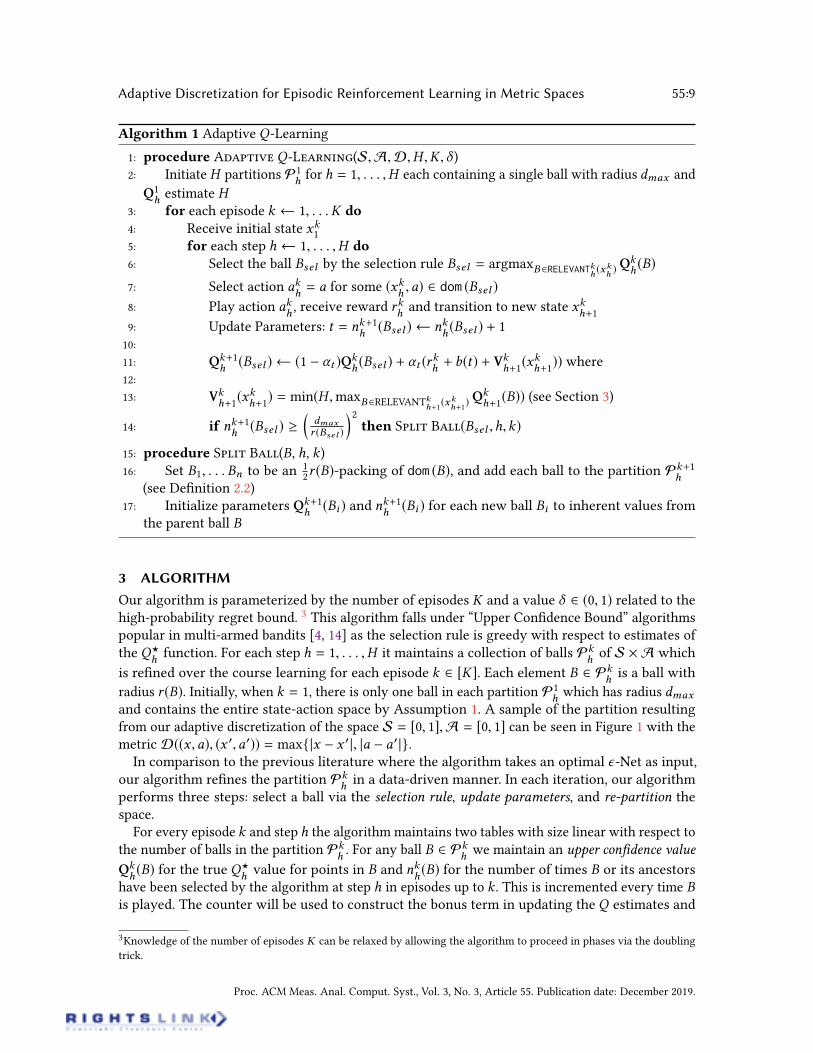
Algorithm 1 Adaptive Q-Learning
1: procedure A QL(S,A,D,H ,K , )2: Initiate H partitions P1
hfor h = 1, . . . ,H each containing a single ball with radius dmax and
Q1hestimate H
3: for each episode k 1, . . .K do
4: Receive initial state xk15: for each step h 1, . . . ,H do
6: Select the ball Bsel by the selection rule Bsel = argmaxB2RELEVANTkh(xkh) Q
kh(B)
7: Select action akh= a for some (xk
h,a) 2 dom (Bsel )
8: Play action akh, receive reward rk
hand transition to new state xk
h+1
9: Update Parameters: t = nk+1h
(Bsel ) nkh(Bsel ) + 1
10:
11: Qk+1h
(Bsel ) (1 t )Qkh(Bsel ) + t (r
kh+ b(t) + Vk
h+1(xk
h+1)) where
12:
13: Vkh+1
(xkh+1
) = min(H ,maxB2RELEVANTkh+1
(xkh+1
) Qkh+1
(B)) (see Section 3)
14: if nk+1h
(Bsel ) dmax
r (Bsel )
2then S B(Bsel ,h,k)
15: procedure S B(B, h, k)16: Set B1, . . . Bn to be an 1
2r (B)-packing of dom (B), and add each ball to the partition Pk+1
h(see Denition 2.2)
17: Initialize parameters Qk+1h
(Bi ) and nk+1h
(Bi ) for each new ball Bi to inherent values fromthe parent ball B
3 ALGORITHM
Our algorithm is parameterized by the number of episodes K and a value 2 (0, 1) related to thehigh-probability regret bound. 3 This algorithm falls under “Upper Condence Bound” algorithmspopular in multi-armed bandits [4, 14] as the selection rule is greedy with respect to estimates ofthe Q?
hfunction. For each step h = 1, . . . ,H it maintains a collection of balls Pk
hof S A which
is rened over the course learning for each episode k 2 [K]. Each element B 2 Pkhis a ball with
radius r (B). Initially, when k = 1, there is only one ball in each partition P1hwhich has radius dmax
and contains the entire state-action space by Assumption 1. A sample of the partition resultingfrom our adaptive discretization of the space S = [0, 1],A = [0, 1] can be seen in Figure 1 with themetric D((x ,a), (x 0,a0)) = max|x x 0 |, |a a0 |.In comparison to the previous literature where the algorithm takes an optimal -Net as input,
our algorithm renes the partition Pkhin a data-driven manner. In each iteration, our algorithm
performs three steps: select a ball via the selection rule, update parameters, and re-partition thespace.
For every episode k and step h the algorithm maintains two tables with size linear with respect tothe number of balls in the partition Pk
h. For any ball B 2 Pk
hwe maintain an upper condence value
Qkh(B) for the true Q?
hvalue for points in B and nk
h(B) for the number of times B or its ancestors
have been selected by the algorithm at step h in episodes up to k . This is incremented every time Bis played. The counter will be used to construct the bonus term in updating the Q estimates and
3Knowledge of the number of episodes K can be relaxed by allowing the algorithm to proceed in phases via the doubling
trick.
Proc. ACM Meas. Anal. Comput. Syst., Vol. 3, No. 3, Article 55. Publication date: December 2019.
55:10 Sean R. Sinclair, Siddhartha Banerjee, and Christina Lee Yu
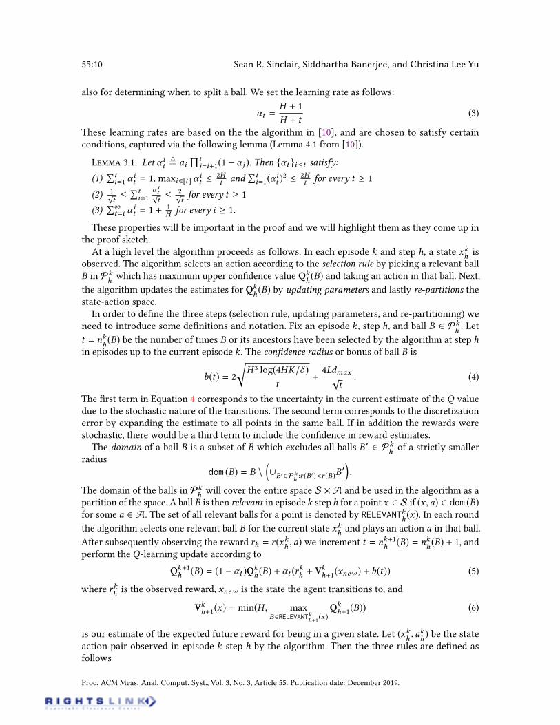
also for determining when to split a ball. We set the learning rate as follows:
t =H + 1
H + t(3)
These learning rates are based on the the algorithm in [10], and are chosen to satisfy certainconditions, captured via the following lemma (Lemma 4.1 from [10]).
L 3.1. Let it , aiŒt
j=i+1(1 j ). Then t it satisfy:
(1)Õt
i=1 it = 1, maxi 2[t ]
it 2H
tand
Õti=1(
it )2 2H
tfor every t 1
(2) 1pt Õt
i=1 itpt 2p
tfor every t 1
(3)Õ1
t=i it = 1 + 1
Hfor every i 1.
These properties will be important in the proof and we will highlight them as they come up inthe proof sketch.At a high level the algorithm proceeds as follows. In each episode k and step h, a state xk
his
observed. The algorithm selects an action according to the selection rule by picking a relevant ballB in Pk
hwhich has maximum upper condence value Qk
h(B) and taking an action in that ball. Next,
the algorithm updates the estimates for Qkh(B) by updating parameters and lastly re-partitions the
state-action space.In order to dene the three steps (selection rule, updating parameters, and re-partitioning) we
need to introduce some denitions and notation. Fix an episode k , step h, and ball B 2 Pkh. Let
t = nkh(B) be the number of times B or its ancestors have been selected by the algorithm at step h
in episodes up to the current episode k . The condence radius or bonus of ball B is
b(t) = 2
rH 3 log(4HK/ )
t+
4Ldmaxpt. (4)
The rst term in Equation 4 corresponds to the uncertainty in the current estimate of the Q valuedue to the stochastic nature of the transitions. The second term corresponds to the discretizationerror by expanding the estimate to all points in the same ball. If in addition the rewards werestochastic, there would be a third term to include the condence in reward estimates.The domain of a ball B is a subset of B which excludes all balls B0 2 Pk
hof a strictly smaller
radius
dom (B) = B \[B02Pk
h:r (B0)<r (B)B
0.
The domain of the balls in Pkhwill cover the entire space S A and be used in the algorithm as a
partition of the space. A ball B is then relevant in episode k steph for a point x 2 S if (x ,a) 2 dom (B)for some a 2 A. The set of all relevant balls for a point is denoted by RELEVANT
kh(x). In each round
the algorithm selects one relevant ball B for the current state xkhand plays an action a in that ball.
After subsequently observing the reward rh = r (xkh,a) we increment t = nk+1
h(B) = nk
h(B) + 1, and
perform the Q-learning update according to
Qk+1h (B) = (1 t )Qk
h(B) + t (rkh + V
kh+1(xnew ) + b(t)) (5)
where rkhis the observed reward, xnew is the state the agent transitions to, and
Vkh+1(x) = min(H , max
B2RELEVANTkh+1
(x )Qkh+1(B)) (6)
is our estimate of the expected future reward for being in a given state. Let (xkh,ak
h) be the state
action pair observed in episode k step h by the algorithm. Then the three rules are dened asfollows
Proc. ACM Meas. Anal. Comput. Syst., Vol. 3, No. 3, Article 55. Publication date: December 2019.
Adaptive Discretization for Episodic Reinforcement Learning in Metric Spaces 55:11
• selection rule: Select a relevant ball B for xkhwith maximal value of Qk
h(B) (breaking ties
arbitrarily). Select any action a to play such that (xkh,a) 2 dom (B). This is similar to the
greedy “upper condence algorithms” for multi-armed bandits.• update parameters: Increment nk
h(B) by 1, and update the Qk
h(B) value for the selected ball
given the observed reward according to Equation 5.• re-partition the space: Let B denote the selected ball and r (B) denote its radius. We splitwhen nk+1
h(B) (dmax/r (B))
2. We then cover dom (B) with new balls B1, . . . ,Bn which form
an 12r (B)-Net of dom (B). We call B the parent of these new balls and each child ball inherits
all values from its parent. We then add the new balls B1, . . . ,Bn to Pkhto form the partition
for the next episode Pk+1h
. 4
See Algorithm 1 for the pseudocode. The full version of the pseudocode is in Appendix B. As areference, see Table 1 in the appendix for a list of notation used.
4 PERFORMANCE GUARANTEES
We provide three main forms of performance guarantees: uniform (i.e., worst-case) regret boundswith arbitrary starting states, rened metric-specic regret bounds, and sample-complexity guar-antees for learning a policy. We close the section with a lower-bound analysis of these results,showing that our results are optimal up to logarithmic factors and a factor of H 2.
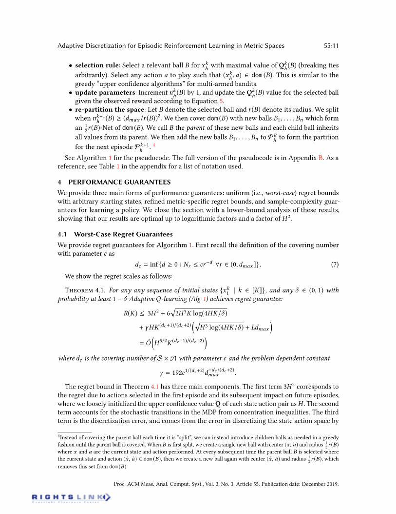
4.1 Worst-Case Regret Guarantees
We provide regret guarantees for Algorithm 1. First recall the denition of the covering numberwith parameter c as
dc = infd 0 : Nr crd ∀r 2 (0,dmax ]. (7)
We show the regret scales as follows:
T 4.1. For any any sequence of initial states xk1 | k 2 [K], and any 2 (0, 1) with
probability at least 1 Adaptive Q-learning (Alg 1) achieves regret guarantee:
R(K) 3H 2+ 6
p2H 3K log(4HK/ )
+ HK (dc+1)/(dc+2)p
H 3 log(4HK/ ) + Ldmax
= O
H 5/2K (dc+1)/(dc+2)
where dc is the covering number of S A with parameter c and the problem dependent constant
= 192c1/(dc+2)ddc /(dc+2)max .
The regret bound in Theorem 4.1 has three main components. The rst term 3H 2 corresponds tothe regret due to actions selected in the rst episode and its subsequent impact on future episodes,where we loosely initialized the upper condence valueQ of each state action pair asH . The secondterm accounts for the stochastic transitions in the MDP from concentration inequalities. The thirdterm is the discretization error, and comes from the error in discretizing the state action space by
4Instead of covering the parent ball each time it is “split”, we can instead introduce children balls as needed in a greedy
fashion until the parent ball is covered. When B is rst split, we create a single new ball with center (x, a) and radius 12 r (B)
where x and a are the current state and action performed. At every subsequent time the parent ball B is selected where
the current state and action (x, a) 2 dom (B), then we create a new ball again with center (x, a) and radius 12 r (B), which
removes this set from dom (B).
Proc. ACM Meas. Anal. Comput. Syst., Vol. 3, No. 3, Article 55. Publication date: December 2019.
55:12 Sean R. Sinclair, Siddhartha Banerjee, and Christina Lee Yu
the adaptive partition. As the partition is adaptive, this term scales in terms of the covering numberof the entire space. Setting = K1/(dc+2), we get the regret of Algorithm 1 as
OH 5/2K (dc+1)/(dc+2)
.
This matches the regret bound from prior work when the metric space S A is taken to be asubset of [0, 1]d , such that the covering dimension is simplyd , the dimension of the metric space [25].For the case of a discrete state-action space with the discrete metric D((s,a), (s 0,a0)) = 1[s=s 0,a=a0],
which has a covering dimension dc = 0, we recover the O(pH 5K) bound from discrete episodic RL
[10].Our experiments in Section 7 shows that the adaptive partitioning saves on time and space
complexity in comparison to the xed Net algorithm [25]. Heuristically, our algorithm achievesbetter regret while reducing the size of the partition. We also see from experiments that the regretseems to scale in terms of the covering properties of the shape of the optimal Q?
hfunction instead
of the entire space similar to the results on contextual bandits in metric spaces [23].Previous work on reinforcement learning in metric spaces give lower bounds on episodic rein-
forcement learning on metric spaces and show that any algorithm must achieve regret where Hscales as H 3/2 and K in terms of K (dc+1)/(dc+2). Because our algorithm achieves worst case regret
O(K (dc+1)/(dc+2)H 5/2) this matches the lower bound up to polylogarithmic factors and a factor of H[23, 25]. More information on the lower bounds is in Section 4.4.
4.2 Metric-Specific Regret Guarantees
The regret bound formulated in Theorem 4.1 is a covering guarantee similar to prior work on banditsin metric spaces [12, 23]. This bound suces for metric spaces where the inequality in the denitionof the covering dimensions Nr crd is tight; a canonical example is when S A = [0, 1]d underthe Euclidean metric, where the covering dimension scales as Nr =
1rd.
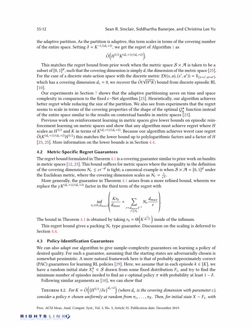
More generally, the guarantee in Theorem 4.1 arises from a more rened bound, wherein wereplace the K (dc+1)/(dc+2) factor in the third term of the regret with
infr02(0,dmax ]
©≠≠≠ Kr0
dmax+
’r=dmax 2
ir r0
Nrdmax
r
™ÆÆÆ.
The bound in Theorem 4.1 is obtained by taking r0 = Θ
K
1dc +2
inside of the inmum.
This regret bound gives a packing Nr type guarantee. Discussion on the scaling is deferred toSection 4.4.
4.3 Policy-Identification Guarantees
We can also adapt our algorithm to give sample-complexity guarantees on learning a policy ofdesired quality. For such a guarantee, assuming that the starting states are adversarially chosen issomewhat pessimistic. A more natural framework here is that of probably approximately correct(PAC) guarantees for learning RL policies [29]. Here, we assume that in each episode k 2 [K], wehave a random initial state X k
1 2 S drawn from some xed distribution F1, and try to nd theminimum number of episodes needed to nd an -optimal policy with probability at least 1 .
Following similar arguments as [10], we can show that
T 4.2. For K = O H 5/2/
dc+2(where dc is the covering dimension with parameter c),
consider a policy chosen uniformly at random from 1, . . . ,K . Then, for initial state X F1, with
Proc. ACM Meas. Anal. Comput. Syst., Vol. 3, No. 3, Article 55. Publication date: December 2019.
Adaptive Discretization for Episodic Reinforcement Learning in Metric Spaces 55:13
probability at least 1 , the policy obeys
V?
1 (X ) V 1 (X ) .
Note that in the above guarantee, both X and are random. The proof is deferred to Appendix D
4.4 Lower Bounds
Existing lower bounds for this problem have been established previously in the discrete tabularsetting [10] and in the contextual bandit literature [23].
Jin et al. [10] show the following for discrete spaces.
T 4.3 (P T 3 [10]). For any algorithm, there exists anH -episodic
discrete MDP with S states and A actions such that for any K , the algorithm’s regret is Ω(H 3/2pSAK).
This shows that our scaling in terms of H is o by a linear factor. As analyzed in [10], we believethat using Bernstein’s inequality instead of Hoeding’s inequality to better manage the variance ofthe Qk
h(B) estimates of a ball will allow us to recover H 2 instead of H 5/2.
Existing lower bounds for learning in continuous spaces have been established in the contextualbandit literature. A contextual bandit instance is characterized by a context space S, action spaceA, and reward function r : S A ! [0, 1]. The agent interacts in rounds, where in each roundthe agent observes an arbitrary initial context x , either drawn from a distribution or specied byan adversary, and the agent subsequently picks an action a 2 A, and receives reward r (x ,a). Thisis clearly a simplication of an episodic MDP where the number of steps H = 1 and the transitionkernel Ph(· | x ,a) is independent of x and a. Lower bounds presented in [12, 23] show that thescaling in terms of Nr in this general regret bound is optimal.
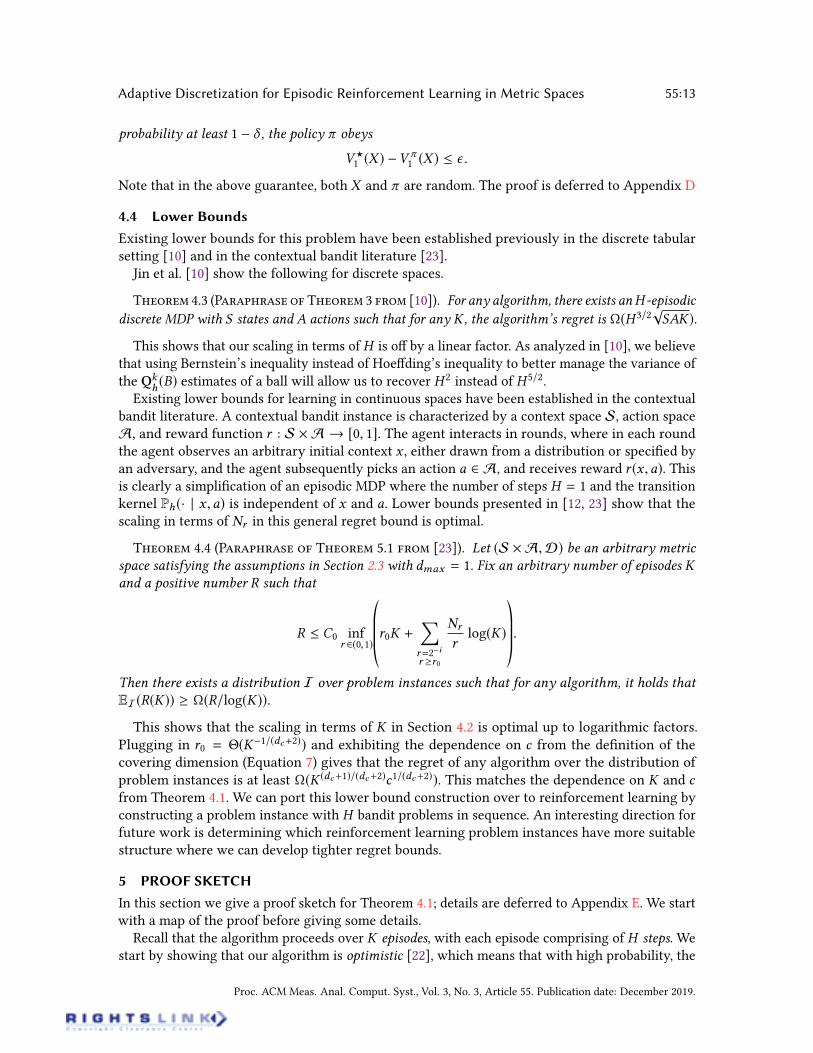
T 4.4 (P T 5.1 [23]). Let (S A,D) be an arbitrary metric
space satisfying the assumptions in Section 2.3 with dmax = 1. Fix an arbitrary number of episodes K
and a positive number R such that
R C0 infr 2(0,1)
©≠≠≠r0K +’r=2ir r0
Nr
rlog(K)
™ÆÆÆ.Then there exists a distribution I over problem instances such that for any algorithm, it holds that
EI(R(K)) Ω(R/log(K)).
This shows that the scaling in terms of K in Section 4.2 is optimal up to logarithmic factors.Plugging in r0 = Θ(K1/(dc+2)) and exhibiting the dependence on c from the denition of thecovering dimension (Equation 7) gives that the regret of any algorithm over the distribution ofproblem instances is at least Ω(K (dc+1)/(dc+2)c1/(dc+2)). This matches the dependence on K and cfrom Theorem 4.1. We can port this lower bound construction over to reinforcement learning byconstructing a problem instance with H bandit problems in sequence. An interesting direction forfuture work is determining which reinforcement learning problem instances have more suitablestructure where we can develop tighter regret bounds.
5 PROOF SKETCH
In this section we give a proof sketch for Theorem 4.1; details are deferred to Appendix E. We startwith a map of the proof before giving some details.
Recall that the algorithm proceeds over K episodes, with each episode comprising of H steps. Westart by showing that our algorithm is optimistic [22], which means that with high probability, the
Proc. ACM Meas. Anal. Comput. Syst., Vol. 3, No. 3, Article 55. Publication date: December 2019.
55:14 Sean R. Sinclair, Siddhartha Banerjee, and Christina Lee Yu
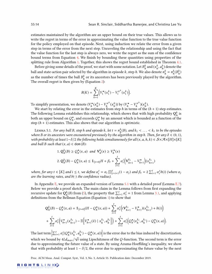
estimates maintained by the algorithm are an upper bound on their true values. This allows us towrite the regret in terms of the error in approximating the value function to the true value functionfor the policy employed on that episode. Next, using induction we relate the error from a givenstep in terms of the error from the next step. Unraveling the relationship and using the fact thatthe value function for the last step is always zero, we write the regret as the sum of the condencebound terms from Equation 4. We nish by bounding these quantities using properties of thesplitting rule from Algorithm 1. Together, this shows the regret bound established in Theorem 4.1.
Before giving some details of the proof, we start with some notation. LetBkhand (xk
h,ak
h) denote the
ball and state-action pair selected by the algorithm in episode k , step h. We also denote nkh= nk
h(Bk
h)
as the number of times the ball Bkhor its ancestors has been previously played by the algorithm.
The overall regret is then given by (Equation 2):
R(K) =
K’k=1
V?
1 (xk1 ) V k
1 (xk1 ).
To simplify presentation, we denote (V?
h(xk
h) V k
h(xk
h)) by (V?
hV k
h)(xk
h).
We start by relating the error in the estimates from step h in terms of the (h + 1) step estimates.The following Lemma establishes this relationship, which shows that with high probability Qk
his
both an upper bound on Q?
h, and exceeds Q?
hby an amount which is bounded as a function of the
step (h + 1) estimates. This also shows that our algorithm is optimistic.
L 5.1. For any ball B, step h and episode k , let t = nkh(B), and k1 < . . . < kt to be the episodes
where B or its ancestors were encountered previously by the algorithm in step h. Then, for any 2 (0, 1),with probability at least 1/2 the following holds simultaneously for all (x ,a,h,k) 2 SA[H ][K]and ball B such that (x ,a) 2 dom (B):
1.Qkh(B) Q?
h (x ,a) and Vkh(x) V
?
h (x)
2.Qkh(B) Q
?
h (x ,a) 1[t=0]H + t +
t’i=1
it
Vkih+1V?
h+1
(x
kih+1
)
where, for any t 2 [K] and i t , we dene ti = iŒt
j=i+1(1 j ) and t = 2Õt
i=1 ti b(i) (where j
are the learning rates, and b(·) the condence radius).
In Appendix E, we provide an expanded version of Lemma 5.1 with a detailed proof (Lemma E.7).Below we provide a proof sketch. The main claim in the Lemma follows from rst expanding therecursive update for Qk
h(B) from (5), the property that
Õti=1
it = 1 from Lemma 3.1, and applying
denitions from the Bellman Equation (Equation 1) to show that
Qkh(B) Q
?
h (x ,a) = 1[t=0](H Q?
h (x ,a)) +
t’i=1
it
(V
kih+1V?
h+1)(xkih+1
) + b(i)
+
t’i=1
it
V?
h+1(xkih+1
) EhV?
h+1(x) | xkih,a
kih
i +
t’i=1
it
Q?
h (xkih,a
kih) Q?
h (x ,a).
The last termÕt
i=1 it (Q
?
h(x
kih,a
kih) Q?
h(x ,a))
is the error due to the bias induced by discretization,which we bound by 4Ldmax/
pt using Lipschitzness of theQ-function. The second term is the error
due to approximating the future value of a state. By using Azuma-Hoeding’s inequality, we showthat with probability at least 1 /2, the error due to approximating the future value by the next
Proc. ACM Meas. Anal. Comput. Syst., Vol. 3, No. 3, Article 55. Publication date: December 2019.
Adaptive Discretization for Episodic Reinforcement Learning in Metric Spaces 55:15
state as opposed to computing the expectation is bounded above byt’i=1
it
V?
h+1(xkih+1
) EhV?
h+1(x) | xkih,a
kih
i 2
rH 3 log(4HK/ )
t.
The nal inequalities in Lemma 5.1 follow by the denition of b(i), t , and substituting the aboveinequalities to the expression for Qk
h(B) Q?
h(x ,a).
By Lemma 5.1, with high probability, Vkh(x) V?
h(x), such that the terms within the summation
of the regret (V?
1 (xk1 ) V k
1 (xk1 )) can be upper bounded by (Vk1 V k
1 )(xk1 ) to show that
R(K) K’k=1
(Vk
1 V k
1 )(xk1 ).
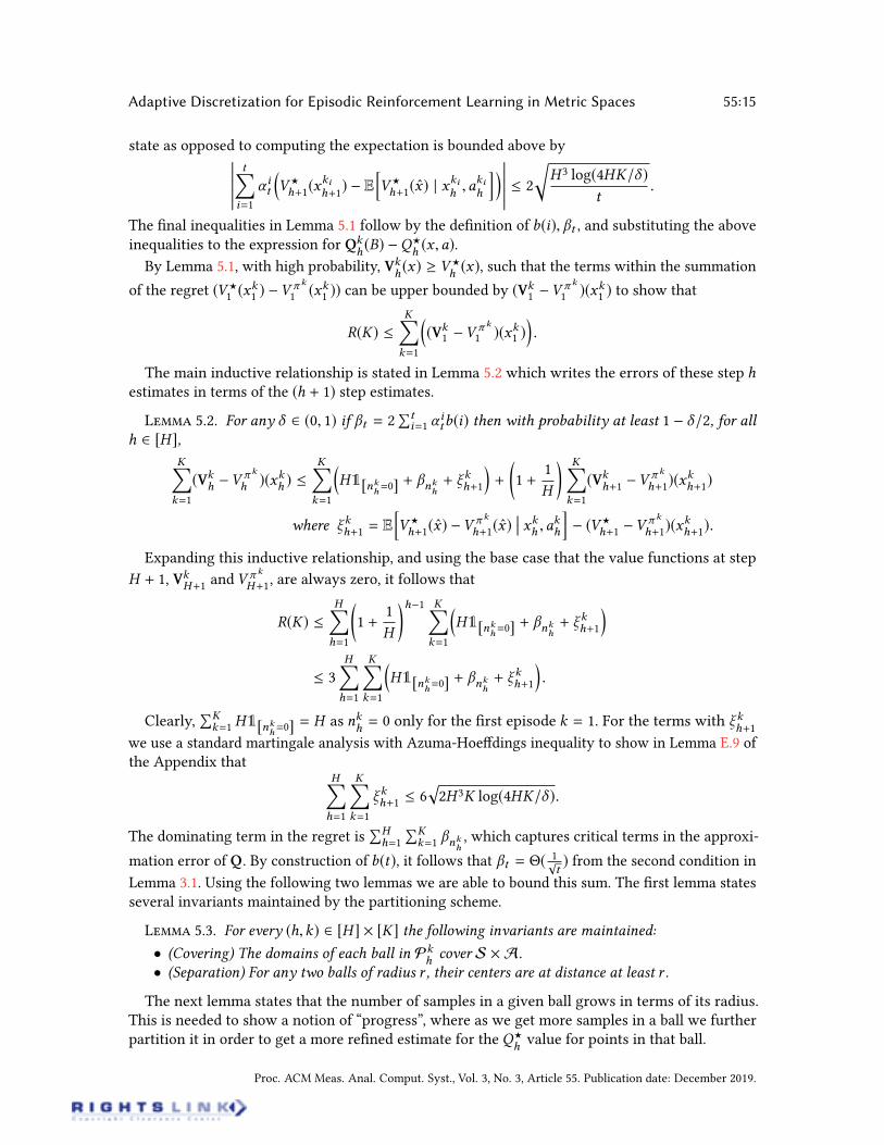
The main inductive relationship is stated in Lemma 5.2 which writes the errors of these step hestimates in terms of the (h + 1) step estimates.
L 5.2. For any 2 (0, 1) if t = 2Õt
i=1 itb(i) then with probability at least 1 /2, for all
h 2 [H ],
K’k=1
(Vkh V
k
h )(xkh ) K’k=1
H1[nk
h=0] + nk
h
+ kh+1
+
1 +
1
H
K’k=1
(Vkh+1 V
k
h+1)(xkh+1)
where kh+1 = EhV?
h+1(x) V k
h+1(x) xkh ,akh i (V?
h+1 V k
h+1)(xkh+1).
Expanding this inductive relationship, and using the base case that the value functions at step
H + 1, VkH+1
and V k
H+1, are always zero, it follows that
R(K) H’h=1
1 +
1
H
h1 K’k=1
H1[nk
h=0] + nk
h
+ kh+1
3
H’h=1
K’k=1
H1[nk
h=0] + nk
h
+ kh+1
.
Clearly,ÕK
k=1H1[nkh=0] = H as nk
h= 0 only for the rst episode k = 1. For the terms with k
h+1
we use a standard martingale analysis with Azuma-Hoedings inequality to show in Lemma E.9 ofthe Appendix that
H’h=1
K’k=1
kh+1 6p2H 3K log(4HK/ ).
The dominating term in the regret isÕHh=1
ÕKk=1 nk
h
, which captures critical terms in the approxi-
mation error of Q. By construction of b(t), it follows that t = Θ( 1pt) from the second condition in
Lemma 3.1. Using the following two lemmas we are able to bound this sum. The rst lemma statesseveral invariants maintained by the partitioning scheme.
L 5.3. For every (h,k) 2 [H ] [K] the following invariants are maintained:
• (Covering) The domains of each ball in Pkhcover S A.
• (Separation) For any two balls of radius r , their centers are at distance at least r .
The next lemma states that the number of samples in a given ball grows in terms of its radius.This is needed to show a notion of “progress”, where as we get more samples in a ball we furtherpartition it in order to get a more rened estimate for the Q?
hvalue for points in that ball.
Proc. ACM Meas. Anal. Comput. Syst., Vol. 3, No. 3, Article 55. Publication date: December 2019.
55:16 Sean R. Sinclair, Siddhartha Banerjee, and Christina Lee Yu
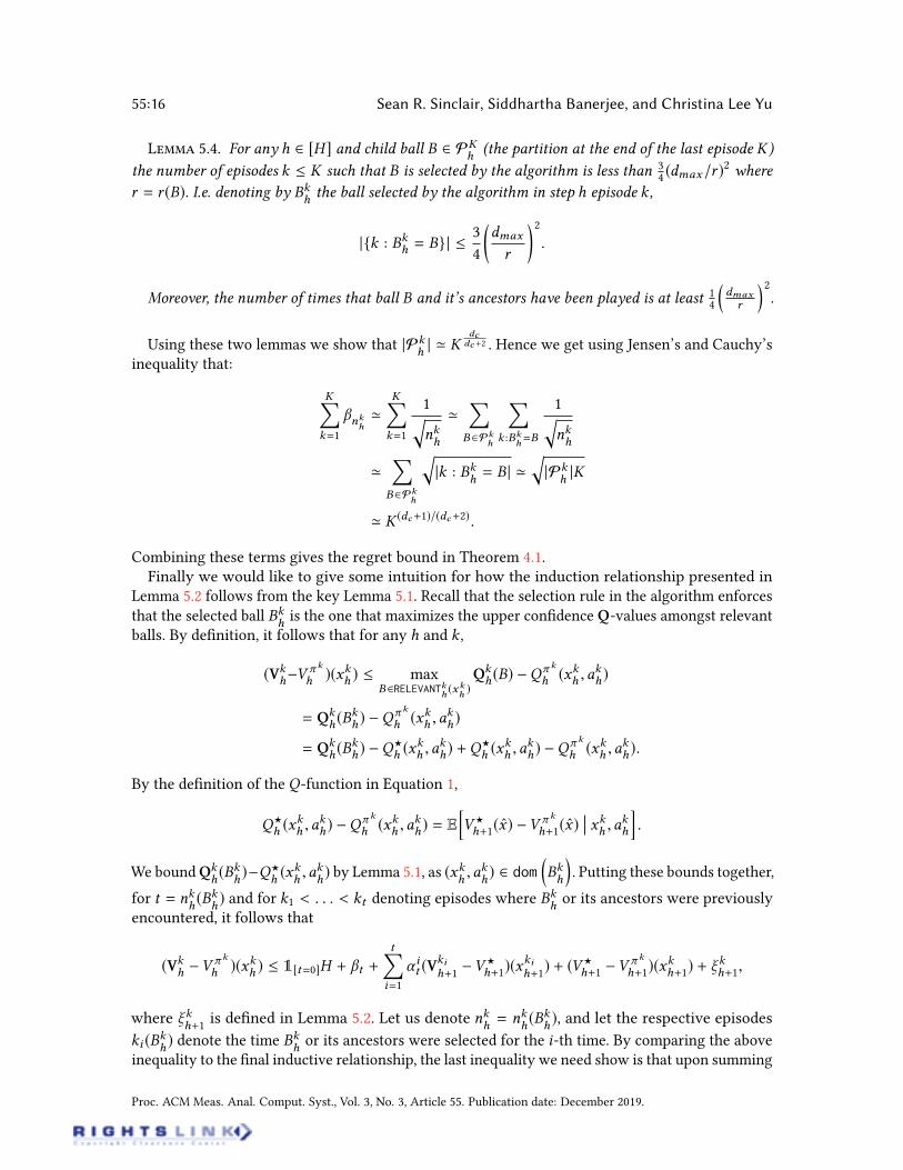
L 5.4. For any h 2 [H ] and child ball B 2 PKh(the partition at the end of the last episode K)
the number of episodes k K such that B is selected by the algorithm is less than 34(dmax/r )
2 where
r = r (B). I.e. denoting by Bkhthe ball selected by the algorithm in step h episode k ,
|k : Bkh = B| 3
4
dmax
r
2.
Moreover, the number of times that ball B and it’s ancestors have been played is at least 14
dmax
r
2.
Using these two lemmas we show that |Pkh| ' K
dc
dc +2 . Hence we get using Jensen’s and Cauchy’sinequality that:
K’k=1
nkh
'K’k=1
1qnkh
'’B2Pk
h
’k :Bk
h=B
1qnkh
'’B2Pk
h
q|k : Bk
h= B | '
q|Pk
h|K
' K (dc+1)/(dc+2).
Combining these terms gives the regret bound in Theorem 4.1.Finally we would like to give some intuition for how the induction relationship presented in
Lemma 5.2 follows from the key Lemma 5.1. Recall that the selection rule in the algorithm enforcesthat the selected ball Bk
his the one that maximizes the upper condence Q-values amongst relevant
balls. By denition, it follows that for any h and k ,
(VkhV
k
h )(xkh ) maxB2RELEVANTk
h(xkh)Qkh(B) Q
k
h (xkh ,akh)
= Qkh(B
kh ) Q
k
h (xkh ,akh)
= Qkh(B
kh ) Q
?
h (xkh ,a
kh) +Q
?
h (xkh ,a
kh) Q
k
h (xkh ,akh).
By the denition of the Q-function in Equation 1,
Q?
h (xkh ,a
kh) Q
k
h (xkh ,akh) = E
hV?
h+1(x) V k
h+1(x) xkh ,akh i .
We boundQkh(Bk
h)Q?
h(xk
h,ak
h) by Lemma 5.1, as (xk
h,ak
h) 2 dom
Bkh
. Putting these bounds together,
for t = nkh(Bk
h) and for k1 < . . . < kt denoting episodes where Bk
hor its ancestors were previously
encountered, it follows that
(Vkh V
k
h )(xkh ) 1[t=0]H + t +
t’i=1
it (Vkih+1V?
h+1)(xkih+1
) + (V?
h+1 V k
h+1)(xkh+1) +
kh+1,
where kh+1
is dened in Lemma 5.2. Let us denote nkh= nk
h(Bk
h), and let the respective episodes
ki (Bkh) denote the time Bk
hor its ancestors were selected for the i-th time. By comparing the above
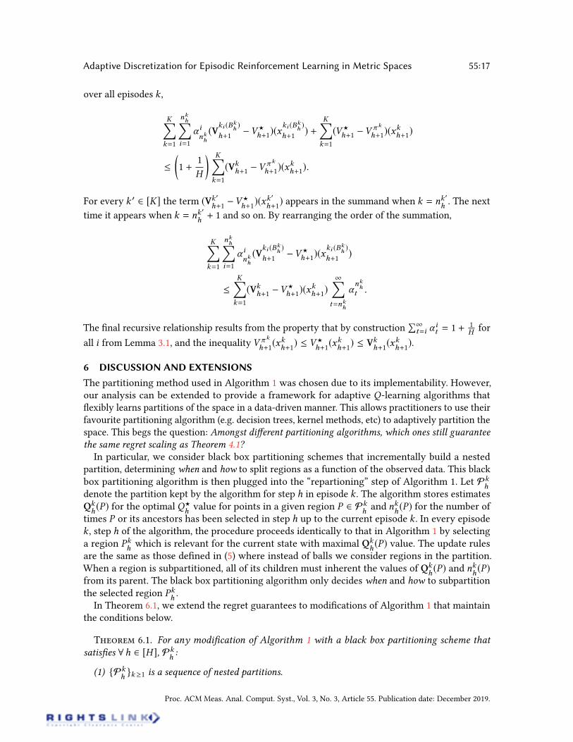
inequality to the nal inductive relationship, the last inequality we need show is that upon summing
Proc. ACM Meas. Anal. Comput. Syst., Vol. 3, No. 3, Article 55. Publication date: December 2019.
Adaptive Discretization for Episodic Reinforcement Learning in Metric Spaces 55:17
over all episodes k ,
K’k=1
nkh’
i=1
inkh
(Vki (B
k
h)
h+1V?
h+1)(xki (B
k
h)
h+1) +
K’k=1
(V?
h+1 V k
h+1)(xkh+1)
1 +
1
H
K’k=1
(Vkh+1 V
k
h+1)(xkh+1).
For every k 0 2 [K] the term (Vk 0
h+1V?
h+1)(xk
0
h+1) appears in the summand when k = nk
0
h. The next
time it appears when k = nk0
h+ 1 and so on. By rearranging the order of the summation,
K’k=1
nkh’
i=1
inkh
(Vki (B
k
h)
h+1V?
h+1)(xki (B
k
h)
h+1)
K’k=1
(Vkh+1 V
?
h+1)(xkh+1)
1’t=nk
h
nkh
t .
The nal recursive relationship results from the property that by constructionÕ1
t=i it = 1 + 1
Hfor
all i from Lemma 3.1, and the inequality V k
h+1(xk
h+1) V?
h+1(xk
h+1) Vk
h+1(xk
h+1).
6 DISCUSSION AND EXTENSIONS
The partitioning method used in Algorithm 1 was chosen due to its implementability. However,our analysis can be extended to provide a framework for adaptive Q-learning algorithms thatexibly learns partitions of the space in a data-driven manner. This allows practitioners to use theirfavourite partitioning algorithm (e.g. decision trees, kernel methods, etc) to adaptively partition thespace. This begs the question: Amongst dierent partitioning algorithms, which ones still guarantee
the same regret scaling as Theorem 4.1?
In particular, we consider black box partitioning schemes that incrementally build a nestedpartition, determining when and how to split regions as a function of the observed data. This blackbox partitioning algorithm is then plugged into the “repartioning” step of Algorithm 1. Let Pk
hdenote the partition kept by the algorithm for step h in episode k . The algorithm stores estimatesQkh(P) for the optimal Q?
hvalue for points in a given region P 2 Pk
hand nk
h(P) for the number of
times P or its ancestors has been selected in step h up to the current episode k . In every episodek , step h of the algorithm, the procedure proceeds identically to that in Algorithm 1 by selectinga region Pk
hwhich is relevant for the current state with maximal Qk
h(P) value. The update rules
are the same as those dened in (5) where instead of balls we consider regions in the partition.When a region is subpartitioned, all of its children must inherent the values of Qk
h(P) and nk
h(P)
from its parent. The black box partitioning algorithm only decides when and how to subpartitionthe selected region Pk
h.
In Theorem 6.1, we extend the regret guarantees to modications of Algorithm 1 that maintainthe conditions below.
T 6.1. For any modication of Algorithm 1 with a black box partitioning scheme that
satises ∀h 2 [H ], Pkh:
(1) Pkhk1 is a sequence of nested partitions.
Proc. ACM Meas. Anal. Comput. Syst., Vol. 3, No. 3, Article 55. Publication date: December 2019.
55:18 Sean R. Sinclair, Siddhartha Banerjee, and Christina Lee Yu
(2) There exists constants c1 and c2 such that for every h,k and P 2 Pkh
c21
diam (P)2 nkh(P)
c22
diam (P)2.
(3) |PKh| Kdc /(dc+2).
the achieved regret is bounded by O(H 5/2K (dc+1)/(dc+2)).
Our algorithm clearly satises the rst condition. The second condition is veried in Lemma E.1,and the third condition follows from a tighter analysis in Lemma E.10. The only dependence on thepartitioning method used when proving Theorem 4.1 is through these sets of assumptions, and sothe proof follows from a straightforward generalization of the results.Similar generalizations were provided in the contextual bandit setting by [27], although they
only show sublinear regret. The rst condition requires that the partition evolves in a hierarchicalmanner, as could be represented by a tree, where each region of the partition has an associatedparent. Due to the fact that a child inherits its Qk
hestimates from its parent, the recursive update
expansion in Lemma 5.1 still holds. The second condition establishes that the number of times agiven region is selected grows in terms of the square of its diameter. This can be thought of asa bias variance trade-o, as when the number of samples in a given region is large, the varianceterm dominates the bias term and it is advantageous to split the partition to obtain more renedestimates. This assumption is necessary for showing Lemma 5.4. It also enforces that the coarsenessof the partition depends on the density of the observations. The third condition controls the size of
the partition and is used to compute the sumÕK
k=1 nkh
from the proof sketch in Section 5.
This theorem provides a practical framework for developing adaptive Q-learning algorithms.The rst condition is easily satised by picking the partition in an online fashion and splittingthe selected region into sub-regions. The second condition can be checked at every iteration anddetermines when to sub-partition a region. The third condition limits the practitioner from creatingunusually shaped regions. Using these conditions, a practitioner can use any decision tree orpartitioning algorithm that satises these properties to create an adaptive Q-learning algorithm.An interesting future direction is to understand whether dierent partitioning methods leads toprovable instance-specic gains.
7 EXPERIMENTS
7.1 Experimental Set up
We compare the performance ofQ-learning with Adaptive Discretization (Algorithm 1) to Net BasedQ-Learning [25] on two canonical problems to illustrate the advantage of adaptive discretizationcompared to uniform mesh. On both problems the state and action space are taken to be S = A =
[0, 1] and the metric the product metric, i.e. D((x ,a), (x 0,a0)) = max|x x 0 |, |a a0 |. This choiceof metric results in a rectangular partition of S A = [0, 1]2 allowing for simpler implementationand easy comparison of the partitions used by the algorithms. We focus on problems which have atwo-dimensional state-action space to provide a proof of concept of the adaptive discretizationsconstructed by the algorithm. These examples have more structure than the worst-case bound, butprovide intuition on the partition “zooming” into important parts of the space. More simulationresults are available with the code on github at https://github.com/seanrsinclair/AdaptiveQLearning.
Oil Discovery. This problem, adapted from [16], is a continuous variant of the popular ‘GridWorld’ game. It comprises of an agent (or agents) surveying a 1D map in search of hidden “oildeposits”. The world is endowed with an unknown survey function f (x) which encodes the oildeposit at each location x . For agents to move to a new location they must pay a cost proportional
Proc. ACM Meas. Anal. Comput. Syst., Vol. 3, No. 3, Article 55. Publication date: December 2019.
Adaptive Discretization for Episodic Reinforcement Learning in Metric Spaces 55:19
to the distance moved; moreover, surveying the land produces noisy estimates of the true value ofthat location.We consider an MDP where S = A = [0, 1] represent the current and future locations of
the agent. The time-invariant transition kernel (i.e., homogeneous for all h 2 [H ]) is dened viaPh(x
0 | x ,a) = 1[x 0=a], signifying that the agent moves to their chosen location. Rewards are givenby rh(x ,a) = max0, f (a)+ |x a |, where is independent sub-Gaussian noise and f (a) 2 [0, 1]is the survey value of the location a (the max ensures rewards are in [0, 1]).We choose the survey function f (x) to be either f (x) = e |xc | or f (x) = 1 (x c)2 where
c 2 [0, 1] is the location of the oil well and is a smoothing parameter, which can be tuned toadjust the Lipschitz constant.
Ambulance Relocation. This is a widely-studied stochastic variant of the above problem [3].Consider an ambulance navigating an environment and trying to position itself in a region withhigh predicted service requests. The agent interacts with the environment by rst choosing alocation to station the ambulance, paying a cost to travel to that location. Next, an ambulancerequest is realized, drawn from a xed distribution, after which the ambulance must travel to meetthe demand at the random location.Formally, we consider an MDP with S = A = [0, 1] encoding the current and future locations
of the ambulance. The transition kernels are dened via Ph(x0 |x ,a) Fh , where Fh denotes the
request distribution for time step h. The reward is rh(x0 |x ,a) = 1 [c |x a | + (1 c)|x 0 a |]; here,
c 2 [0, 1] models the trade-os between the cost of relocation (often is less expensive) and cost oftraveling to meet the demand.
For the arrival distribution Fh we consider Beta(5, 2) and Uniform(0, 1) to illustrate dispersed andconcentrated request distributions. We also analyzed the eect of changing the arrival distributionover time (e.g. Figure 1). We compare the RL methods to two heuristics: “No Movement”, where theambulance pays the cost of traveling to the request, but does not relocate after that, and “Median”,where the ambulance always relocates to the median of the observed requests. Each heuristic isnear-optimal respectively at the two extreme values of c .
7.2 Adaptive Tree Implementation
We used a tree data structure to implement the partition Pkhof Algorithm 1. We maintain a tree for
every step h 2 [H ] to signify our partition of S A = [0, 1]2. Each node in the tree corresponds toa rectangle of the partition, and contains algorithmic information such as the estimate of the Qk
hvalue at the node. Each node has an associated center (x ,a) and radius r . We store a list of (possiblyfour) children for covering the region which arises when splitting a ball.To implement the selection rule we used a recursive algorithm which traverses through all the
nodes in the tree, checks each node if the given state xkhis contained in the node, and if so recursively
checks the children to obtain the maximum Qkhvalue. This speeds up computation by following
the tree structure instead of linear traversal. For additional savings we implemented this using amax-heap.For Net Based Q-Learning, based on the recommendation in [25], we used a xed -Net of the
state-action space, with = (KH )1/4 (since d = 2). An example of the discretization can be seen inFigure 1 where each point in the discretization is the center of a rectangle.
7.3 Experimental Results
Oil Discovery. First we consider the oil problem with survey function f (a) = e |ac | where = 1. This results in a sharp reward function. Heuristically, the optimal policy can be seen totake the rst step to travel to the maximum reward at c and then for each subsequent step stay
Proc. ACM Meas. Anal. Comput. Syst., Vol. 3, No. 3, Article 55. Publication date: December 2019.
55:20 Sean R. Sinclair, Siddhartha Banerjee, and Christina Lee Yu
0 1000 2000 3000 4000 5000
Episode
0
1
2
3
4
5
ObservedReward
Comparison of Observed Rewards
Adaptive
Epsilon Net
0 1000 2000 3000 4000 5000
Episode
0
100
200
300
400
500
600
700
800
SizeofPartition
Comparison of Size of Partition
0.0 0.2 0.4 0.6 0.8 1.0
State Space
0.0
0.2
0.4
0.6
0.8
1.0
ActionSpace
Adaptive Discretization for Step 2
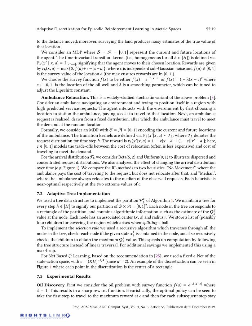
Fig. 2. Comparison of the observed rewards, size of partition, and discretization for the uniformmesh [25] and
our adaptive discretization algorithms, on the oil discovery problem with survey function f (x) = e |x0.75 | .The transition kernel is Ph (x
0 | x ,a) = 1[x 0=a] and reward function is r (x ,a) = (1 e |a0.75 | |x a |)+ (seeSection 7.1). The adaptive algorithm quickly learns the location of the optimal point 0.75 and creates a fine
partition of the space around the optimal.
0 500 1000 1500 2000
Episode
0
1
2
3
4
5
ObservedReward
Comparison of Observed Rewards
Adaptive
Epsilon Net
Median
No Movement
0 500 1000 1500 2000
Episode
100
200
300
400
500
SizeofPartition
Comparison of Size of Partition
0.0 0.2 0.4 0.6 0.8 1.0
State Space
0.0
0.2
0.4
0.6
0.8
1.0
ActionSpace
Adaptive Discretization for Step 2
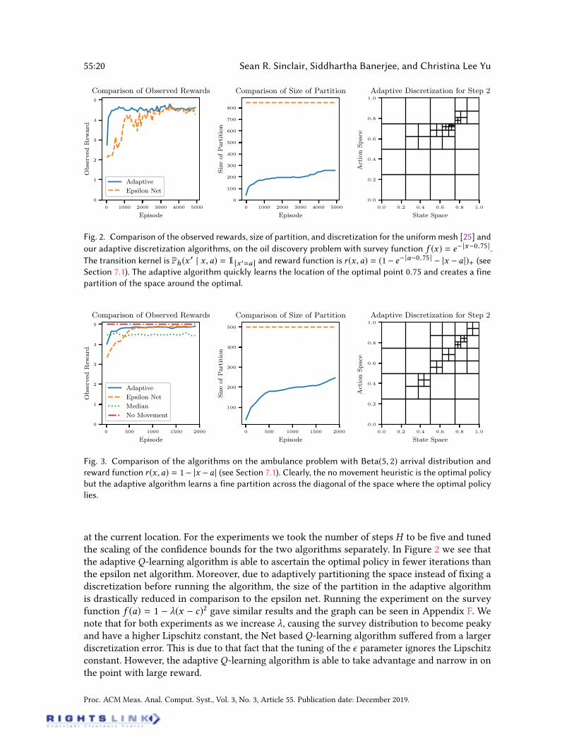
Fig. 3. Comparison of the algorithms on the ambulance problem with Beta(5, 2) arrival distribution and
reward function r (x ,a) = 1 |x a | (see Section 7.1). Clearly, the no movement heuristic is the optimal policy
but the adaptive algorithm learns a fine partition across the diagonal of the space where the optimal policy
lies.
at the current location. For the experiments we took the number of steps H to be ve and tunedthe scaling of the condence bounds for the two algorithms separately. In Figure 2 we see thatthe adaptive Q-learning algorithm is able to ascertain the optimal policy in fewer iterations thanthe epsilon net algorithm. Moreover, due to adaptively partitioning the space instead of xing adiscretization before running the algorithm, the size of the partition in the adaptive algorithmis drastically reduced in comparison to the epsilon net. Running the experiment on the surveyfunction f (a) = 1 (x c)2 gave similar results and the graph can be seen in Appendix F. Wenote that for both experiments as we increase , causing the survey distribution to become peakyand have a higher Lipschitz constant, the Net based Q-learning algorithm suered from a largerdiscretization error. This is due to that fact that the tuning of the parameter ignores the Lipschitzconstant. However, the adaptive Q-learning algorithm is able to take advantage and narrow in onthe point with large reward.
Proc. ACM Meas. Anal. Comput. Syst., Vol. 3, No. 3, Article 55. Publication date: December 2019.
Adaptive Discretization for Episodic Reinforcement Learning in Metric Spaces 55:21
Ambulance Routing. We consider the ambulance routing problem with arrival distributionF = Beta(5, 2). The time horizon H is again taken to be ve. We implemented two additionalheuristics for the problem to serve as benchmarks. The rst is the “No Movement” heuristic. Thisalgorithm takes the action to never move, and pays the entire cost of traveling to service the arrival.The second, “Median” heuristic takes the action to travel to the estimated median of the distributionbased on all past arrivals. For the case when c = 1 no movement is the optimal algorithm. For c = 0
the optimal will be to travel to the median.After running the algorithms with c = 1 the adaptive Q-learning algorithm is better able to
learn the stationary policy of not moving from the current location, as there is only a cost ofmoving to the action. The rewards observed by each algorithm is seen in Figure 3. In this case,the discretization (for step h = 2) shows that the adaptive Q-learning algorithm maintains a nerpartition across the diagonal where the optimal policy lives. Running the algorithm for c < 1 showsthat the adaptive Q-learning algorithm has a ner discretization around (x ,a) = (0.7, 0.7), where0.7 is the approximate median of a Beta(5, 2) distribution. The algorithm keeps a ne discretizationboth around where the algorithm frequently visits, but also places of high reward. For c < 1 and thearrival distribution F = Uniform[0, 1] the results were similar and the graphs are in Appendix F.The last experiment was to analyze the algorithms when the arrival distribution changes over
time (e.g. over steps h). In Figure 1 we took c = 0 and shifting arrival distributions Fh where F1 =
Uniform(0, 1/4),F2 = Uniform(1/4, 1/2),F3 = Uniform(1/2, 3/4),F4 = Uniform(3/4, 1), and F5 =
Uniform(1/2 0.05, 1/2+ 0.05). In the gure, the color corresponds to theQ?
hvalue of that specic
state-action pair, where green corresponds to a larger value for the expected future rewards. Theadaptive algorithm was able to converge faster to the optimal policy than the uniform meshalgorithm. Moreover, the discretization observed from the Adaptive Q-Learning algorithm followsthe contours of the Q-function over the space. This shows the intuition behind the algorithmof storing a ne partition across near-optimal parts of the space, and a coarse partition acrosssub-optimal parts.
8 CONCLUSION
We presented an algorithm for model-free episodic reinforcement learning on continuous stateaction spaces that uses data-driven discretization to adapt to the shape of the optimal policy. Underthe assumption that the optimal Q? function is Lipschitz, the algorithm achieves regret boundsscaling in terms of the covering dimension of the metric space.Future directions include relaxing the requirements on the metric, such as considering weaker
versions of the Lipschitz condition. In settings where the metric may not be known a priori, it wouldbe meaningful to be able to estimate the distance metric from data over the course of executinng ofthe algorithm. Lastly, we hope to characterize problems where adaptive discretization outperformsuniform mesh.
ACKNOWLEDGMENTS
We gratefully acknowledge funding from the NSF under grants ECCS-1847393 and DMS-1839346,and the ARL under grant W911NF-17-1-0094.
Proc. ACM Meas. Anal. Comput. Syst., Vol. 3, No. 3, Article 55. Publication date: December 2019.
55:22 Sean R. Sinclair, Siddhartha Banerjee, and Christina Lee Yu
REFERENCES
[1] Peter Auer, Thomas Jaksch, and Ronald Ortner. 2009. Near-optimal Regret Bounds for Reinforcement Learning. In
Advances in Neural Information Processing Systems 21, D. Koller, D. Schuurmans, Y. Bengio, and L. Bottou (Eds.). Curran
Associates, Inc., 89–96. http://papers.nips.cc/paper/3401-near-optimal-regret-bounds-for-reinforcement-learning.pdf
[2] Mohammad Gheshlaghi Azar, Ian Osband, and Rémi Munos. 2017. Minimax Regret Bounds for Reinforcement Learning.
In Proceedings of the 34th International Conference on Machine Learning - Volume 70 (ICML’17). JMLR.org, 263–272.
http://dl.acm.org/citation.cfm?id=3305381.3305409
[3] Luce Brotcorne, Gilbert Laporte, and Frederic Semet. 2003. Ambulance location and relocation models. European
journal of operational research 147, 3 (2003), 451–463.
[4] Sébastien Bubeck, Nicolo Cesa-Bianchi, et al. 2012. Regret analysis of stochastic and nonstochastic multi-armed bandit
problems. Foundations and Trends® in Machine Learning 5, 1 (2012), 1–122.
[5] Sébastien Bubeck, Gilles Stoltz, Csaba Szepesvári, and Rémi Munos. 2009. Online optimization in X-armed bandits. In
Advances in Neural Information Processing Systems. 201–208.
[6] Joshua Comden, Sijie Yao, Niangjun Chen, Haipeng Xing, and Zhenhua Liu. 2019. Online Optimization in Cloud
Resource Provisioning: Predictions, Regrets, and Algorithms. Proc. ACM Meas. Anal. Comput. Syst. 3, 1, Article 16
(March 2019), 30 pages. https://doi.org/10.1145/3322205.3311087
[7] Kefan Dong, YuanhaoWang, Xiaoyu Chen, and Liwei Wang. 2019. Q-learning with UCB Exploration is Sample Ecient
for Innite-Horizon MDP. arXiv preprint arXiv:1901.09311 (2019).
[8] Simon S Du, Yuping Luo, Ruosong Wang, and Hanrui Zhang. 2019. Provably Ecient Q -learning with Function
Approximation via Distribution Shift Error Checking Oracle. arXiv preprint arXiv:1906.06321 (2019).
[9] Alison L Gibbs and Francis Edward Su. 2002. On choosing and bounding probability metrics. International statistical
review 70, 3 (2002), 419–435.
[10] Jin C, JordanM.I, Allen-Zhu Z, Bubeck S, and NeurIPS 2018 32nd Conference on Neural Information Processing Systems.
2018. Is Q-learning provably ecient? Adv. neural inf. proces. syst. Advances in Neural Information Processing Systems
2018-December (2018), 4863–4873. OCLC: 8096900528.
[11] Sham Kakade, Michael Kearns, and John Langford. 2003. Exploration in Metric State Spaces. In Proceedings of the
Twentieth International Conference on International Conference on Machine Learning (ICML’03). AAAI Press, 306–312.
http://dl.acm.org/citation.cfm?id=3041838.3041877
[12] Robert Kleinberg, Aleksandrs Slivkins, and Eli Upfal. 2019. Bandits and Experts in Metric Spaces. J. ACM 66, 4, Article
30 (May 2019), 77 pages. https://doi.org/10.1145/3299873
[13] K. Lakshmanan, Ronald Ortner, and Daniil Ryabko. 2015. Improved Regret Bounds for Undiscounted Continuous
Reinforcement Learning. In Proceedings of the 32nd International Conference onMachine Learning (Proceedings of Machine
Learning Research), Francis Bach and David Blei (Eds.), Vol. 37. PMLR, Lille, France, 524–532. http://proceedings.mlr.
press/v37/lakshmanan15.html
[14] Tor Lattimore and Csaba Szepesvári. 2018. Bandit algorithms. preprint (2018).
[15] Hongzi Mao, Mohammad Alizadeh, Ishai Menache, and Srikanth Kandula. 2016. Resource Management with Deep
Reinforcement Learning. In Proceedings of the 15th ACM Workshop on Hot Topics in Networks (HotNets ’16). ACM, New
York, NY, USA, 50–56. https://doi.org/10.1145/3005745.3005750
[16] Winter Mason and Duncan J Watts. 2012. Collaborative learning in networks. Proceedings of the National Academy of
Sciences 109, 3 (2012), 764–769.
[17] Ronald Ortner. 2013. Adaptive aggregation for reinforcement learning in average reward Markov decision processes.
Annals of Operations Research 208, 1 (01 Sep 2013), 321–336. https://doi.org/10.1007/s10479-012-1064-y
[18] Ronald Ortner and Daniil Ryabko. 2012. Online Regret Bounds for Undiscounted Continuous Reinforce-
ment Learning. In Advances in Neural Information Processing Systems 25, F. Pereira, C. J. C. Burges,
L. Bottou, and K. Q. Weinberger (Eds.). Curran Associates, Inc., 1763–1771. http://papers.nips.cc/paper/
4666-online-regret-bounds-for-undiscounted-continuous-reinforcement-learning.pdf
[19] Ian Osband and Benjamin Van Roy. 2014. Model-based Reinforcement Learning and the Eluder Dimen-
sion. In Advances in Neural Information Processing Systems 27, Z. Ghahramani, M. Welling, C. Cortes, N. D.
Lawrence, and K. Q. Weinberger (Eds.). Curran Associates, Inc., 1466–1474. http://papers.nips.cc/paper/
5245-model-based-reinforcement-learning-and-the-eluder-dimension.pdf
[20] Martin L. Puterman. 1994. Markov Decision Processes: Discrete Stochastic Dynamic Programming (1st ed.). John Wiley &
Sons, Inc., New York, NY, USA.
[21] Devavrat Shah and Qiaomin Xie. 2018. Q-learning with Nearest Neighbors. In Advances in Neural Information
Processing Systems 31, S. Bengio, H. Wallach, H. Larochelle, K. Grauman, N. Cesa-Bianchi, and R. Garnett (Eds.). Curran
Associates, Inc., 3111–3121. http://papers.nips.cc/paper/7574-q-learning-with-nearest-neighbors.pdf
[22] Max Simchowitz and Kevin Jamieson. 2019. Non-Asymptotic Gap-Dependent Regret Bounds for Tabular MDPs.
arXiv:cs.LG/1905.03814
Proc. ACM Meas. Anal. Comput. Syst., Vol. 3, No. 3, Article 55. Publication date: December 2019.
Adaptive Discretization for Episodic Reinforcement Learning in Metric Spaces 55:23
[23] Aleksandrs Slivkins. 2015. Contextual Bandits with Similarity Information. Journal of machine learning research :
JMLR. 15, 2 (2015), 2533–2568. OCLC: 5973068319.
[24] Aleksandrs Slivkins. 2019. Introduction to Multi-Armed Bandits. arXiv:cs.LG/1904.07272
[25] Zhao Song and Wen Sun. 2019. Ecient Model-free Reinforcement Learning in Metric Spaces. arXiv:1905.00475 [cs,
stat] (May 2019). http://arxiv.org/abs/1905.00475 arXiv: 1905.00475.
[26] Richard S Sutton and Andrew G Barto. 2018. Reinforcement learning: An introduction. MIT press.
[27] Tianyu Wang, Weicheng Ye, Dawei Geng, and Cynthia Rudin. 2019. Towards Practical Lipschitz Stochastic Bandits.
arXiv e-prints, Article arXiv:1901.09277 (Jan 2019), arXiv:1901.09277 pages. arXiv:stat.ML/1901.09277
[28] Nirandika Wanigasekara and Christina Lee Yu. 2019. Nonparametric Contextual Bandits in an Unknown Metric Space.
arXiv:cs.LG/1908.01228
[29] Christopher John Cornish Hellaby Watkins. 1989. Learning from delayed rewards. (1989).
[30] Lin Yang and Mengdi Wang. 2019. Sample-Optimal Parametric Q-Learning Using Linearly Additive Features. In
International Conference on Machine Learning. 6995–7004.
[31] Lin F Yang, Chengzhuo Ni, and Mengdi Wang. 2019. Learning to Control in Metric Space with Optimal Regret. arXiv
preprint arXiv:1905.01576 (2019).
[32] Lin F. Yang and Mengdi Wang. 2019. Reinforcement Leaning in Feature Space: Matrix Bandit, Kernels, and Regret
Bound. arXiv:1905.10389 [cs, stat] (May 2019). http://arxiv.org/abs/1905.10389 arXiv: 1905.10389.
Proc. ACM Meas. Anal. Comput. Syst., Vol. 3, No. 3, Article 55. Publication date: December 2019.
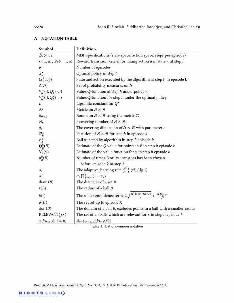
55:24 Sean R. Sinclair, Siddhartha Banerjee, and Christina Lee Yu
A NOTATION TABLE
Symbol Denition
S,A,H MDP specications (state space, action space, steps per episode)
rh(x ,a) , Ph(· | x ,a) Reward/transition kernel for taking action a in state x at step h
K Number of episodes
?
hOptimal policy in step h
(xkh,ak
h) State and action executed by the algorithm at step h in episode k
∆(S) Set of probability measures on S
V h(·),Q
h(·, ·) Value/Q-function at step h under policy
V?
h(·),Q?
h(·, ·) Value/Q-function for step h under the optimal policy
L Lipschitz constant for Q?
D Metric on S Admax Bound on S A using the metric D
Nr r covering number of S Adc The covering dimension of S A with parameter c
Pkh
Partition of S A for step h in episode k
Bkh
Ball selected by algorithm in step h episode k
Qkh(B) Estimate of the Q value for points in B in step h episode k
Vkh(x) Estimate of the value function for x in step h episode k
nkh(B) Number of times B or its ancestors has been chosen
before episode k in step h
t The adaptive learning rate H+1H+t
(cf. Alg 1)
it iŒt
j=i+1(1 j )diam (B) The diameter of a set B
r (B) The radius of a ball B
b(t) The upper condence term, 2
qH 3 log(4HK/ )
t+
4LDmaxpt
R(K) The regret up to episode K
dom (B) The domain of a ball B, excludes points in a ball with a smaller radius
RELEVANTkh(x) The set of all balls which are relevant for x in step h episode k
E[Vh+1(x) | x ,a] ExPh (· |x,a)[Vh+1(x)]
Table 1. List of common notation
Proc. ACM Meas. Anal. Comput. Syst., Vol. 3, No. 3, Article 55. Publication date: December 2019.
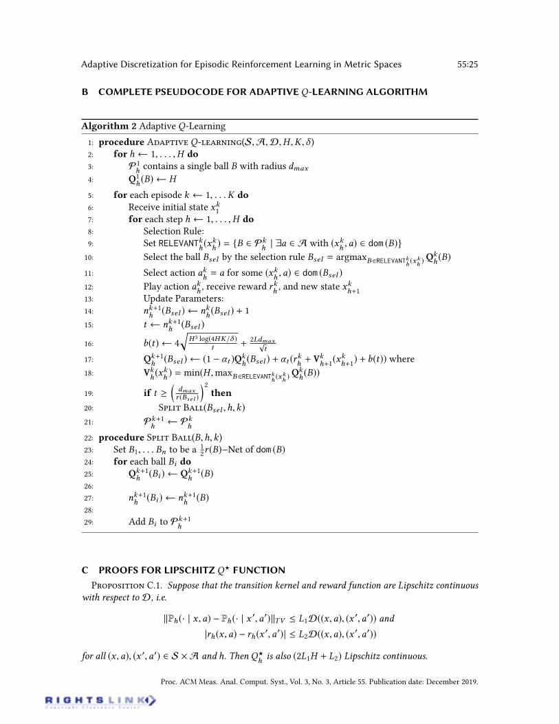
Adaptive Discretization for Episodic Reinforcement Learning in Metric Spaces 55:25
B COMPLETE PSEUDOCODE FOR ADAPTIVE Q-LEARNING ALGORITHM
Algorithm 2 Adaptive Q-Learning
1: procedure A Q(S,A,D,H ,K , )2: for h 1, . . . ,H do
3: P1hcontains a single ball B with radius dmax
4: Q1h(B) H
5: for each episode k 1, . . .K do
6: Receive initial state xk17: for each step h 1, . . . ,H do
8: Selection Rule:9: Set RELEVANTk
h(xk
h) = B 2 Pk
h| ∃a 2 A with (xk
h,a) 2 dom (B)
10: Select the ball Bsel by the selection rule Bsel = argmaxB2RELEVANTkh(xkh) Q
kh(B)
11: Select action akh= a for some (xk
h,a) 2 dom (Bsel )
12: Play action akh, receive reward rk
h, and new state xk
h+113: Update Parameters:14: nk+1
h(Bsel ) nk
h(Bsel ) + 1
15: t nk+1h
(Bsel )
16: b(t) 4
qH 3 log(4HK/ )
t+
2Ldmaxpt
17: Qk+1h
(Bsel ) (1 t )Qkh(Bsel ) + t (r
kh+ Vk
h+1(xk
h+1) + b(t)) where
18: Vkh(xk
h) = min(H ,maxB2RELEVANTk
h(xkh) Q
kh(B))
19: if t dmax
r (Bsel )
2then
20: S B(Bsel ,h,k)
21: Pk+1h Pk
h
22: procedure S B(B,h,k)23: Set B1, . . . Bn to be a 1
2r (B)Net of dom (B)
24: for each ball Bi do25: Qk+1
h(Bi ) Qk+1
h(B)
26:
27: nk+1h
(Bi ) nk+1h
(B)
28:
29: Add Bi to Pk+1h
C PROOFS FOR LIPSCHITZ Q? FUNCTION
P C.1. Suppose that the transition kernel and reward function are Lipschitz continuous
with respect to D, i.e.
kPh(· | x ,a) Ph(· | x 0,a0)kTV L1D((x ,a), (x 0,a0)) and
|rh(x ,a) rh(x 0,a0)| L2D((x ,a), (x 0,a0))
for all (x ,a), (x 0,a0) 2 S A and h. Then Q?
his also (2L1H + L2) Lipschitz continuous.
Proc. ACM Meas. Anal. Comput. Syst., Vol. 3, No. 3, Article 55. Publication date: December 2019.
55:26 Sean R. Sinclair, Siddhartha Banerjee, and Christina Lee Yu
P. We use the denition of Q?
h. Indeed, for any h 2 [H ],
|Q?
h (x ,a) Q?
h (x0,a0)| = |rh(x ,a) rh(x 0,a0) + E
V?
h+1(x) | x ,a E
V?
h+1(x) | x0,a0
|.
However, noting that both Ph(· | x ,a) and Ph(· | x0,a0) are absolutely continuous with respect
to the base measure = 12(Ph(· | x ,a) + Ph(· | x
0,a0)) we are able to deconstruct the dierence in
expectations with respect to the Radon-Nikodym derivatives as the measures are -nite. Hence,
|rh(x ,a) rh(x 0,a0)| +π
V?
h+1(x)dPh(x | x ,a) π
V?
h+1(x)dPh(x | x 0,a0)
L2D((x ,a), (x 0,a0)) +
π
V?
h+1(x)dPh(x | x ,a)
d(x)d(x)
πV?
h+1(x)dPh(x | x 0,a0)
d(x)d(x)
L2D((x ,a), (x 0,a0)) +
π|V?
h+1(x)|
dPh(x | x ,a)
d(x) dPh(x | x 0,a0)
d(x)
d(x) L2D((x ,a), (x 0,a0)) + kV?
h+1k1π dPh(x | x ,a)
d(x) dPh(x | x 0,a0)
d(x)
d(x) L2D((x ,a), (x 0,a0)) + H
dPh(· | x ,a)d dPh(· | x
0,a0)
d
1
= L2D((x ,a), (x 0,a0)) + 2H kPh(· | x ,a) Ph(· | x 0,a0)kTV L2D((x ,a), (x 0,a0)) + 2HL1D((x ,a), (x 0,a0))
where we have used the fact that the total variation distance is twice the L1 distance of theRadon-Nikodym derivatives.
Now we further assume that S is a separable and compact metric space with metric dS . We alsoassume that D((x ,a), (x 0,a)) CdS(x ,x
0) where we assume C = 1 for simplicity.As a preliminary we begin with the following lemma.
L C.2. Suppose that f : S A ! R is L Lipschitz and uniformly bounded. Then (x) =
supa2A f (x ,a) is also L Lipschitz.
P. Fix any x1 and x2 2 S. First notice that | f (x1,a) f (x2,a)| LD((x1,a), (x2,a)) LdS(x1,x2) by choice of product metric.
Thus, for any a 2 A we have that
f (x1,a) f (x2,a) + LdS(x1,x2) (x2) + LdS(x1,x2).
However, as this is true for any a 2 A we see that (x1) (x2) + LdS(x1,x2). Swapping the roleof x1 and x2 in the inequality shows |(x1) (x2)| LdS(x1,x2) as needed.
We will use this and properties of the Wasserstein metric from [9] to give conditions on the Q?
function to be Lipschitz. First notice the denition of the Wasserstein metric on a separable metricspace via:
dW (µ, ) = sup
π
f dµ π
f d
: k f kL 1
where k f kL is the smallest Lipschitz constant of the function f and µ and are measures on thespace S.
Proc. ACM Meas. Anal. Comput. Syst., Vol. 3, No. 3, Article 55. Publication date: December 2019.
Adaptive Discretization for Episodic Reinforcement Learning in Metric Spaces 55:27
P C.3. Suppose that the transition kernel is Lipschitz with respect to the Wasserstein
metric and the reward function is Lipschitz continuous, i.e.
|rh(x ,a) rh(x 0,a0)| L1D((x ,a), (x0,a0))
dW (Ph(· | x ,a),Ph(· | x0,a0)) L2D((x ,a), (x
0,a0))
for all (x ,a), (x 0,a0) 2 S A and h where dW is the Wasserstein metric. Then Q?
hand V?
hare both
(ÕHh
i=0 L1Li2) Lipschitz continuous.
P. We show this by induction on h. For the base case when h = H +1 thenV?
H+1= Q?
H+1= 0
and so the result trivially follows.Similarly when h = H then by Equation 1 we have that Q?
H(x ,a) = rH (x ,a). Thus, |Q
?
H(x ,a)
Q?
H(x 0,a0)| = |rH (x ,a) rH (x
0,a0)| L1D((x ,a), (x 0,a0)) by assumption. Moreover, V?
H(x) =
maxa2A Q?
H(x ,a) is L1 Lipschitz by Equation 1 and Lemma C.2.
For the step case we assume that Q?
h+1and V?
h+1are both
ÕHh1i=0 L1L
i2 Lipschitz and show the
result for Q?
hand V?
h. Indeed,
|Q?
h (x ,a) Q?
h (x0,a0)| = |rh(x ,a) rh(x 0,a0) + E
V?
h+1(x) | x ,a E
V?
h+1(x) | x0a0
|
|rh(x ,a) rh(x 0,a0)| + |EV?
h+1(x) | x ,a E
V?
h+1(x) | x0a0
|
L1D((x ,a), (x 0,a0)) +
π
V?
h+1(x)dPh(x | x ,a) π
V?
h+1(x)dPh(x | x 0,a0)
Now denoting by K =
ÕHh1i=0 L1L
i2 by the induction hypothesis and the properties of Wasserstein
metric (Equation 3 from [9]) we have that
|Q?
h (x ,a) Q?
h (x0,a0)| L1D((x ,a), (x 0,a0))
+ K
π
1
KV?
h+1(x)dPh(x | x ,a) π
1
KV?
h+1(x)dPh(x | x 0,a0)
L1D((x ,a), (x 0,a0)) + KdW (Ph(· | x ,a),Ph(· | x
0,a0))
L1D((x ,a), (x 0,a0)) + KL2D((x ,a), (x 0,a0))
= (L1 + KL2)D((x ,a), (x 0,a0)).
Noting that by denition of K we have L1 + KL2 =ÕHh1
i=0 L1Li2. To show that V?
his also Lipschitz
we simply use Lemma C.2.
D POLICY-IDENTIFICATION GUARANTEES PROOF
T D.1. For K = O H 5/2/
dc+2(where dc is the covering dimension with parameter c),
consider a policy chosen uniformly at random from 1, . . . ,K . Then, for an initial state X F1,
with probability at least 1 , the policy obeys
V?
1 (X ) V 1 (X ) .
Note that in the above guarantee, both X and are random.
Proc. ACM Meas. Anal. Comput. Syst., Vol. 3, No. 3, Article 55. Publication date: December 2019.
55:28 Sean R. Sinclair, Siddhartha Banerjee, and Christina Lee Yu
P. Let X F1 be a random starting state sampled from F1. Then from Markov’s inequalityand the law of total expectation, we have that:
P(V?
1 (X ) V 1 (X ) > c) 1
Kc
K’k=1
E
hV?
1 (X ) V k
1 (X )i
1
KcO
H 5/2K (dc+1)/(dc+2))
= O
H 5/2K
1dc +2
c
!,
where the last inequality follows from the guarantee in Theorem 4.1. Setting c = and K =
O H 5/2/
dc+2in the above expression gives that V?
1 (x) V 1 (x) with probability at least
1 .
E PROOF DETAILS
E.1 Required Lemmas
We start with a collection of lemmas which are required to show Theorem 4.1.The rst two lemmas consider invariants established by the partitioning of the algorithm. These
state that the algorithm maintains a partition of the state-action space at every iteration of thealgorithm, and that the balls of similar radius are suciently apart.
L E.1 (L 5.3 ). For every (h,k) 2 [H ][K] the following invariantsare maintained:
• (Covering) The domains of each ball in Pkhcover S A.
• (Separation) For any two balls of radius r , their centers are at distance at least r.
P. Let (h,k) 2 [H ] [K] be arbitrary.For the covering invariant notice that [B2Pk
h
dom (B) = [B2Pk
h
B where we are implicitly taking
the domain with respect to the partition Pkh. The covering invariant follows then since Pk
hcontains
a ball which covers the entire space S A from the initialization in the algorithm.To show the separation invariant, suppose that B1 and B2 are two balls of radius r . If B1 and B2
share a parent, we note by the splitting rule the algorithm maintains the invariant that the centersare at a distance at least r from each other. Otherwise, suppose without loss of generality that B1 hasparent Bpar and that B2 was activated before B1. The center of B1 is some point (x ,a) 2 dom (Bpar ).It follows then that (x ,a) < dom (B2) by denition of the domain as r (Bpar ) > r (B2). Thus, theircenters are at a distance at least r from each other.
The second property is useful as it maintains that the centers of the balls of radius r form an
rpacking of S A and hence there are at most Npackr Nr balls activated of radius r .
The next theorem gives an analysis on the number of times that a ball of a given radius will beselected by the algorithm. This Lemma also shows the second condition required for a partitioningalgorithm to achieve the regret bound as described in Section 6.
L E.2 (L 5.4 ). For any h 2 [H ] and child ball B 2 PKh
(the
partition at the end of the last episode K) the number of episodes k K such that B is selected by the
algorithm is less than 34(dmax/r )
2 where r = r (B). I.e. denoting by Bkhthe ball selected by the algorithm
in step h episode k ,
|k : Bkh = B| 3
4
dmax
r
2.
Proc. ACM Meas. Anal. Comput. Syst., Vol. 3, No. 3, Article 55. Publication date: December 2019.
Adaptive Discretization for Episodic Reinforcement Learning in Metric Spaces 55:29
Moreover, the number of times that ball B and its ancestors have been played is at least 14
dmax
r
2.
For the case when B is the initial ball which covers the entire space then the number of episodes that
B is selected is only one.
P. Consider an arbitrary h 2 [H ] and child ball B 2 PKhsuch that r (B) = r . Furthermore,
let k be the episode for which ball B was activated. Then Bkh, the ball selected by the algorithm at
step h in episode k is the parent of B. Moreover, if t = nk+1h
(Bkh) is the number of times that Bk
hor
it’s ancestors have been played then t =
dmax
r (Bkh)
2by the activation rule. Also, r (Bk
h) = 2r (B) by the
re-partitioning scheme. Hence, the number of times that B and its ancestors have been played is atleast
t =
dmax
r (Bkh)
!2=
dmax
2r (B)
2=
1
4
dmax
r (B)
2.
The number of episodes that B can be selected (i.e. |k : Bkh= B|) by the algorithm is bounded
above bydmax
r (B)
2
dmax
r (Bkh)
2as this is the number of samples of B required to split the ball by the
partitioning scheme. However, plugging in r (Bkh) = 2r (B) gives
dmax
r (B)
2
dmax
2r (B)
2=
3
4
dmax
r (B)
2
as claimed.Lastly if B is the initial ball which covers the entire space then r (B) = dmax initially and so the
ball is split after it is selected only once.
Next we provide a recursive relationship for the update in Q estimates.
L E.3. For any h,k 2 [H ] [K] and ball B 2 Pkhlet t = nk
h(B) be the number of times that B
or its ancestors were encountered during the algorithm before episode k . Further suppose that B and its
ancestors were encountered at step h of episodes k1 < k2 < . . . < kt < k . By the update rule of Q we
have that:
Qkh (B) = 1[t=0]H +
t’i=1
it
rh(x
kih,a
kih) + V
kih+1
(xkih+1
) + b(i).
P. We show the claim by induction on t = nkh(B).
First suppose that t = 0, i.e. that the ball B has not been encountered before by the algorithm.Then initially Q1
h(B) = H = 1[t=0]H .
Now for the step case we notice that Qkh(B) was last updated at episode kt . kt is either the most
recent episode when ball B was encountered, or the most recent episode when it’s parent wasencountered if B was activated and not yet played. In either case by the update rule (Equation 5)
Proc. ACM Meas. Anal. Comput. Syst., Vol. 3, No. 3, Article 55. Publication date: December 2019.
55:30 Sean R. Sinclair, Siddhartha Banerjee, and Christina Lee Yu
we have
Qkh(B) = (1 t )Qkt
h(B) + t
rh(x
kth,a
kth) + V
kth+1
(xkth+1
) + b(t)
= (1 t )0t1H + (1 t )
t1’i=1
it
rh(x
kih,a
kih) + V
kih+1
(xkih+1
) + b(i)
+ t
rh(x
kth,a
kth) +V
kth+1
(xkth+1
) + b(t)by the induction hypothesis
= 1[t=0]H +
t’i=1
it
rh(x
kih,a
kih) + V
kih+1
(xkih+1
) + b(i)
by denition of it .
The next lemma extends the relationship between the optimal Q value Q?
h(x ,a) for any (x ,a) 2
S A to the estimate of theQ value for any ball B containing (x ,a). For ease of notation we denote(Vk
h(x) V?
h(x)) = (Vk
hV?
h)(x).
L E.4. For any (x ,a,h,k) 2 S A [H ] [K] and ball B 2 Pkhsuch that (x ,a) 2 dom (B)
then if t = nkh(B) and B and its ancestors were previously encountered at step h in episodes k1 < k2 <
. . . < kt < k then
Qkh(B) Q
?
h (x ,a) = 1[t=0](H Q?
h (x ,a)) +
t’i=1
it
(V
kih+1V?
h+1)(xkih+1
) +V?
h+1(xkih+1
)
EhV?
h+1(x) | xkih,a
kih
i+ b(i) +Q?
h (xkih,a
kih) Q?
h (x ,a)
P. Consider any (x ,a) 2 S A and h 2 [H ] arbitrary and an episode k 2 [K]. Furthermore,let B be any ball such that (x ,a) 2 B. First notice by Lemma 3.1 that 1[t=0] +
Õti=1
it = 1 for any
t 0.We show the claim by induction on t = nk
h(B).
For the base case that t = 0 then Qkh(B) = H as it has not been encountered before by the
algorithm. Then
Qkh(B) Q
?
h (x ,a) = H Q?
h (x ,a) = 1[t=0](H Q?
h (x ,a)).
For the step case we use the fact thatÕt
i=1 it + 1[t=0] = 1. Thus, Q?
h(x ,a) =
Õti=1
itQ
?
h(x ,a) +
1[t=0]Q?
h(x ,a). Subtracting this from Qk
h(B) and using Lemma E.3 yields
Qkh(B) Q
?
h (x ,a) = 1[t=0]H +
t’i=1
it
rh(x
kih,a
kih) + V
kih+1
(xkih+1
) + b(i)
1[t=0]Q?
h (x ,a) t’i=1
itQ?
h (x ,a)
= 1[t=0](H Q?
h (x ,a)) +
t’i=1
it
rh(x
kih,a
kih) + V
kih+1
(xkih+1
) + b(i)
+Q?
h (xkih,a
kih) Q?
h (xkih,a
kih) Q?
h (x ,a).
However, using the Bellman Equations (1) we know that
Q?
h (xkih,a
kih) = rh(x
kih,a
kih) + E
hV?
h+1(x) | xkih,a
kih
i.
Proc. ACM Meas. Anal. Comput. Syst., Vol. 3, No. 3, Article 55. Publication date: December 2019.
Adaptive Discretization for Episodic Reinforcement Learning in Metric Spaces 55:31
Using this above we get that
Qkh(B) Q
?
h (x ,a) = 1[t=0](H Q?
h (x ,a)) +
t’i=1
it
Vkih+1
(xkih+1
) EhV?
h+1(x) | xkih,a
kih
i
+ b(i) +Q?
h (xkih,a
kih) Q?
h (x ,a)
= 1[t=0](H Q?
h (x ,a)) +
t’i=1
it
(V
kih+1V?
h+1)(xkih+1
)
+V?
h+1(xkih+1
) EhV?
h+1(x) | xkih,a
kih
i+ b(i) +Q?
h (xkih,a
kih) Q?
h (x ,a).
Consider now V?
h+1(x
kih+1
) EhV?
h+1(x) | x
kih,a
kih
i. We notice that as the next state xki
h+1is drawn
from Ph(· | xkih,a
kih) then E
hV?
h+1(x
kih+1
)i= E
hV?
h+1(x) | x
kih,a
kih
i. Thus, this sequence forms a
martingale dierence sequence and so by Azuma-Hoeding’s inequality we are able to show thefollowing.
L E.5. For all (x ,a,h,k) 2 S A [H ] [K] and for all 2 (0, 1) we have with probability
at least 1 /2 if (x ,a) 2 B for some B 2 Pkhthen for t = nk
h(B) and episodes k1 < k2 < . . . < kt < k
where B and its ancestors were encountered at step h before episode k thent’i=1
it
V?
h+1(xkih+1
) EhV?
h+1(x) | xkih,a
kih
i H
vt2
t’i=1
( it )2 log(4HK/ ).
P. Consider the sequence
ki = min(k,mink : nkh(Ba) = i and Ba is an ancestor of B or B itself).
Clearly ki is the episode for which B or its ancestors were encountered at step h for the i-th time(as once a ball is split it is never chosen by the algorithm again). Setting
Zi = 1[ki k ]V?
h+1(xkih+1
) EhV?
h+1(x) | xkih,a
kih
i then Zi is a martingale dierence sequence with respect to the ltration Fi which we denote asthe information available to the agent up to an including the step ki . Moreover, as the sum of amartingale dierence sequence is a martingale then for any K ,
Õi=1 Zi is a martingale. Noticing
that the dierence between subsequent terms is bounded byH i and Azuma-Hoeding’s inequalitywe see that for a xed K
P©≠’i=1
iZi
H
vt2
’i=1
( i )2 log
4HK
™Æ 1 2 exp
2H 2 Õ
i=1(i )
2 log( 4HK
)
2H 2Õ
i=1(i )
2
!
= 1
2HK.
Since the inequality holds for xed K the the inequality must also hold for the random stoppingtime = t = nk
h(B) K . Moreover, for this stopping time each of the indicator functions will be 1.
Proc. ACM Meas. Anal. Comput. Syst., Vol. 3, No. 3, Article 55. Publication date: December 2019.
55:32 Sean R. Sinclair, Siddhartha Banerjee, and Christina Lee Yu
Taking a union bound over the number of episodes and over all H the result follows. We onlyneed to union bound over the number of episodes instead of the number of balls as the inequalityis satised for all balls not selected in a given round as it inherits its concentration from its parentball because the value for t does not change.We also notice that for t > 0 that
Õti=1(
it )2 2H
tby Lemma 3.1 and so
H
vt2
t’i=1
( it )2 log(4HK/ ) H
r22H
tlog(4HK/ ) = 2
rH 3 log(4HK/ )
t.
The next lemma uses the activation rule and Assumption 2 to bound the dierence between theoptimalQ functions at a point (x ,a) in B from the points sampled in ancestors of B by the algorithm.This corresponds to the accumulation of discretization errors in the algorithm by accumulatingestimates over a ball.
L E.6. For any (x ,a,h,k) 2 S A [H ] [K] and ball B 2 Pkhwith (x ,a) 2 dom (B) if B
and its ancestors were encountered at step h in episodes k1 < k2 < . . . < kt < k where t = nkh(B) then
t’i=1
it
Q?
h (xkih,a
kih) Q?
h (x ,a) 4Ldmaxp
t.
P. Denote by Bkih
as the ball selected in step h of episode ki and nkih
as nkih(B
kih). Then
each Bkih
is an ancestor of B and s both (x ,a) and (xkih,a
kih). Hence by the Lipschitz assumption
(Assumption 2) we have that |Q?
h(x
kih,a
kih) Q?
h(x ,a)| L diam
Bkih
2Lr (B
kih).
However, r (Bkih) dmaxp
i. Indeed, by the re-partition rule we split when n
kih=
dmax
r (Bki
h)
2(and
afterwards Bkih
is not chosen again) and so nkih
dmax
r (Bki
h)
2. Square rooting this gives that
qnkih
dmax
r (Bki
h). However, as nki
h= i we get that r (Bki
h) dmaxp
i. Using this we have that
t’i=1
it
Q?
h (xkih,a
kih) Q?
h (x ,a) t’
i=1
it2Lr (Bkih)
2
t’i=1
itLdmax1pi
4Ldmax1ptby Lemma 3.1.
The next lemma provides an upper and lower bound on the dierence between Qkh(B) and
Q?
h(x ,a) for any (x ,a) 2 dom (B). It also shows that our algorithm is optimistic, in that the estimates
are upper bounds for the true quality and value function for the optimal policy [22].
L E.7 (E L 5.1 ). For any 2 (0, 1) if
t = 2Õt
i=1 itb(i) then
t 8
rH 3 log(4HK/ )
t+ 16
Ldmaxpt
Proc. ACM Meas. Anal. Comput. Syst., Vol. 3, No. 3, Article 55. Publication date: December 2019.
Adaptive Discretization for Episodic Reinforcement Learning in Metric Spaces 55:33
and
t 4
rH 3 log(4HK/ )
t+ 8
Ldmaxpt.
Moreover, with probability at least 1 /2 the following holds simultaneously for all (x ,a,h,k) 2S A [H ] [K] and ball B such that (x ,a) 2 dom (B) where t = nk
h(B) and k1 < . . . < kt are the
episodes where B or its ancestors were encountered previously by the algorithm
0 Qkh(B) Q
?
h (x ,a) 1[t=0]H + t +
t’i=1
it (Vkih+1V?
h+1)(xkih+1
)
P. First consider t = 2Õt
i=1 itb(i). By denition of the bonus term as
b(t) = 2
rH 3 log(4HK/ )
t+ 2
Ldmaxpt
we have the following (where we use Lemma 3.1):
t = 2
t’i=1
itb(i)
= 2
t’i=1
it (2
rH 3 log(4HK/ )
i+ 4
Ldmaxpi
)
4(2
rH 3 log(4HK/ )
t+ 4
Ldmaxpt
)
= 8
rH 3 log(4HK/ )
t+ 16
Ldmaxpt
We can similarly lower-bound the expression by 4
qH 3 log(4HK/ )
t+ 8 Ldmaxp
tusing the lower bound
from Lemma 3.1.We start with the upper bound on Qk
h(B) Q?
h(x ,a). Indeed, by Lemma E.4 we have
Qkh(B) Q
?
h (x ,a) = 1[t=0](H Q?
h (x ,a)) +
t’i=1
it
(V
kih+1V?
h+1)(xkih+1
)
+V?
h+1(xkih+1
) EhV?
h+1(x) | xkih,a
kih
i+ b(i) +Q?
h (xkih,a
kih) Q?
h (x ,a).
However, with probability at least 1 /2 by Lemma E.5 and Lemma E.6 we get
1[t=0]H +
t’i=1
itb(i) + 2
rH 3 log(4HK/ )
t+ 4
Ldmaxpt+
t’i=1
it (Vkih+1V?
h+1)(xkih+1
)
1[t=0]H +
t’i=1
itb(i) +t
2+
t’i=1
it (Vkih+1V?
h+1)(xkih+1
)
Using thatÕt
i=1 itb(i) = t/2 establishes the upper bound.
For the lower bound we show the claim by induction on h = H + 1,H , . . . , 1.Indeed, for the base case when h = H + 1 then Q?
H+1(x ,a) = 0 = Qk
H+1(B) for every k , ball B, and
(x ,a) 2 S A trivially as at the end of the episode the expected future reward is always zero.
Proc. ACM Meas. Anal. Comput. Syst., Vol. 3, No. 3, Article 55. Publication date: December 2019.
55:34 Sean R. Sinclair, Siddhartha Banerjee, and Christina Lee Yu
Now, assuming the claim for h+1we show the claim for h. First consider Vkih+1
(xkih+1
)V?
h+1(x
kih+1
).
We show that Vkih+1
(xkih+1
) V?
h+1(x
kih+1
) 0. By the Bellman Equations (1) we know that
V?
h+1(xkih+1
) = supa2A
Q?
h+1(xkih+1,a) = Q?
h+1(xkih+1,?
h+1(xkih+1
)).
If Vkih+1
(xkih+1
) = H then the inequality trivially follows as V?(xkih+1
) H . Thus by the update
in the algorithm we can assume that Vkih+1
(xkih+1
) = maxB2RELEVANTki
h+1(x
ki
h+1)Qkih(B). Now let B? be
the ball with smallest radius in Pkih+1
such that (xkih+1,?
h+1(x
kih+1
)) 2 B?. Such a ball exists as Pkih+1
covers S A by Lemma E.1. Moreover (xkih+1,?
h+1(x
kih+1
)) 2 domB?
as B? was taken to have the
smallest radius. Thus, Qkih+1
(B?) Q?
h+1(x
kih+1,?
h+1(x
kih+1
)) by the induction hypothesis. Hence wehave that
Vkih+1
(xkih+1
) Qkih+1
(B?) Q?
h+1(xkih+1,?
h+1(xkih+1
)) = V?
h+1(xkih+1
).
Putting all of this together with Lemma E.4 then with probability 1/2we have (using Lemma E.5and denition of t/2) that
Qkh(B) Q
?
h (x ,a) = 1[t=0](H Q?
h (x ,a)) +
t’i=1
it
(V
kih+1V?
h+1)(xkih+1
)
+V?
h+1(xkih+1
) EhV?
h+1(x) | xkih,a
kih
i+ b(i) +Q?
h (xkih,a
kih) Q?
h (x ,a)
t’i=1
it (Vkih+1V?
h+1)(xkih+1
) +t
2 2
pH 3 log(4HK/ )/t 4Ldmaxp
t
t
2 t
2 0
where in the last line we used that Vkih+1
(xkih+1
) V?
h+1(x
kih+1
) from before.
The next Lemma extends the results from Lemma E.7 to lower bounds of VkhV?
hover the entire
state space S.
C E.8. For any 2 (0, 1) with probability at least 1 /2 the following holds simultane-
ously for all (x ,h,k) 2 S [H ] [K]
Vkh(x) V
?
h (x) 0
P. The proof of the lower bound follows from the argument used in the proof of Lemma E.7.
The next lemma uses Azuma-Hoeding’s inequality to bound a martingale dierence sequencewhich arises in the proof of the regret bound.
L E.9. For any 2 (0, 1) with probability at least 1 /2 we have thatH’h=1
K’k=1
EhV?
h+1(x) V k
h+1(x) | xkh ,a
kh
i (V?
h+1(xkh+1) V
k
h+1(xkh ,a
kh))
2p2H 3K log(4HK/ ).
P. First consider Zkh= E
hV?
h+1(x) V k
h+1(x) | xk
h,ak
h
i (V?
h+1(xk
h+1) V k
h+1(xk
h)). Similar to
the proof of Lemma E.5 we notice that Zkhis a martingale dierence sequence due to the fact that
the next state is drawn from the distribution Ph(· | xkh,ak
h). Using that |Zk
h| 2H we have that
Proc. ACM Meas. Anal. Comput. Syst., Vol. 3, No. 3, Article 55. Publication date: December 2019.
Adaptive Discretization for Episodic Reinforcement Learning in Metric Spaces 55:35
P
H’h=1
K’k=1
EhV?
h+1(x) V k
h+1(x) | xkh ,a
kh
i (V?
h+1(xkh+1) V
k
h+1(xkh ,a
kh))
> p8H 3K log(4HK/ )
!
2 exp
8H
3K log(4HK/ )
2HK(2H )2
= 2 exp
8H
3K log(4HK/ )
8H 3K
= 2
4KH /2.
Thus with probability at least 1 /2 we have thatH’h=1
K’k=1
EhV?
h+1(x) V k
h+1(x) | xkh ,a
kh
i (V?
h+1(xkh+1) V
k
h+1(xkh ,a
kh))
p8H 3K log(4HK/ )
as claimed.
This next lemma provides a bound on the sum of errors accumulated from the condence boundst throughout the algorithm. This term gives rise to the Nr covering terms from Theorem 4.1. ThisLemma can also show the third condition required for a partitioning algorithm to achieve the regretbound as described in Section 6.
L E.10. For every h 2 [H ], if Bkhis the ball selected by the algorithm in step h episode k and
nkh= nk
h(Bk
h) then
K’k=1
nkh
32p
H 3 log(4HK/ ) + Ldmax
inf
r02(0,dmax ]
©≠≠≠’
r=dmax 2i
r r0
Nrdmax
r+
Kr0
dmax
™ÆÆÆ.P. Using Lemma E.7,
K’k=1
nkh
K’k=1
8
sH 3 log(4HK/ )
nkh
+ 16Ldmaxq
nkh
16p
H 3 log(4HK/ ) + Ldmax
K’k=1
1qnkh
.
We thus turn our attention toÕK
k=1 1/qnkh. Rewriting the sum in terms of the radius of all balls
activated by the algorithm we get for an arbitrary r0 2 (0,dmax ],
K’k=1
1qnkh
=
’r=dmax 2i
’B2PK
h
r (B)=r
’k :Bk
h=B
1qnkh(B)
=
’r=dmax 2
ir r0
’B2PK
h
r (B)=r
’k :Bk
h=B
1qnkh(B)
+
’r=dmax 2
ir<r0
’B2PK
h
r (B)=r
’k :Bk
h=B
1qnkh(B)
,
Proc. ACM Meas. Anal. Comput. Syst., Vol. 3, No. 3, Article 55. Publication date: December 2019.
55:36 Sean R. Sinclair, Siddhartha Banerjee, and Christina Lee Yu
taking the two cases when r r0 and r < r0 separately. We rst start with r < r0. Then,
’r=dmax 2
ir<r0
’B2PK
h
r (B)=r
’k :Bk
h=B
1qnkh(B)
’
r=dmax 2i
r<r0
’B2PK
h
r (B)=r
’k :Bk
h=B
1q14d2max/r
2
by Lemma E.2
’
r=dmax 2i
r<r0
’B2PK
h
r (B)=r
’k :Bk
h=B
2r0
dmax 2Kr0
dmax
by bounding the number of terms in the sum by the number of episodes K .For the case when r r0 we get
’r=dmax 2
ir r0
’B2PK
h
r (B)=r
’k :Bk
h=B
1qnkh(B)
’
r=dmax 2i
r r0
’B2PK
h
r (B)=r
34
dmax
r
2’i=1
1ri + 1
4
dmax
r
2 by Lemma E.2
’
r=dmax 2i
r r0
’B2PK
h
r (B)=r
π 34
dmax
r
21
1rx + 1
4
dmax
r
2dx
=
’r=dmax 2
ir r0
’B2PK
h
r (B)=r
2dmax
r
’
r=dmax 2i
r r0
2Nrdmax
r
as by Lemma E.1 the centers of balls of radius r are at a distance at least r from each other and thusform an r -packing of S A. Hence, the total number of balls of radius r is at most Nr . Thus weget that (taking the inf over r0 arbitrary):
K’k=1
1qnkh
infr02(0,dmax ]
©≠≠≠’
r=dmax 2i
r r0
2Nrdmax
r+
2Kr0
dmax
™ÆÆÆ.
Proc. ACM Meas. Anal. Comput. Syst., Vol. 3, No. 3, Article 55. Publication date: December 2019.
Adaptive Discretization for Episodic Reinforcement Learning in Metric Spaces 55:37
Plugging this back into the rst inequality gives that
K’k=1
nkh
16p
H 3 log(4HK/ ) + Ldmax
K’k=1
1qnkh
16p
H 3 log(4HK/ ) + Ldmax
inf
r02(0,dmax ]
©≠≠≠’
r=dmax 2i
r r0
2Nrdmax
r+
2Kr0
dmax
™ÆÆÆ
= 32p
H 3 log(4HK/ ) + Ldmax
inf
r02(0,dmax ]
©≠≠≠’
r=dmax 2i
r r0
Nrdmax
r+
Kr0
dmax
™ÆÆÆ.
E.2 Regret Analysis
We start with a lemma which was highlighted in the proof sketch from Section 5.
L E.11 (L 5.2 ). For any 2 (0, 1) if t = 2Õt
i=1 itb(i) then with
probability at least 1 /2, for all h 2 [H ],
K’k=1
(Vkh V
k
h )(xkh ) K’k=1
(H1[nkh=0] + nk
h
+ kh+1) +
1 +
1
H
K’k=1
(Vkh+1 V
k
h+1)(xkh+1).
P L E.11. By equations 6 and 1, and the denition of the selection rule by thealgorithm it follows that for any h and k that
Vkh(x
kh ) V
k
h (xkh ) maxB2RELEVANTk
h(xkh)Qkh(B) Q
k
h (xkh ,akh)
= Qkh(B
kh ) Q
k
h (xkh ,akh)
= Qkh(B
kh ) Q
?
h (xkh ,a
kh) +Q
?
h (xkh ,a
kh) Q
k
h (xkh ,akh).
First, by Equation 1 we know thatQ?
h(xk
h,ak
h)Q k
h(xk
h,ak
h) = E
hV?
h+1(x) V k
h+1(x) | xk
h,ak
h
i. More-
over, as (xkh,ak
h) 2 dom
Bkh
we can use Lemma 5.1 and get for t = nk
h(Bk
h) and episodesk1 < . . . < kt
where Bkhor its ancestors were previously encountered
Qkh(B
kh ) Q
?
h (xkh ,a
kh) +Q
?
h (xkh ,a
kh) Q
k
h (xkh ,akh)
1[t=0]H + t +
t’i=1
it (Vkih+1V?
h+1)(xkih+1
) + EhV?
h+1(x) V k
h+1(x) | xkh ,a
kh
i
1[t=0]H + t +
t’i=1
it (Vkih+1V?
h+1)(xkih+1
) + (V?
h+1 V k
h+1)(xkh+1) +
kh+1
where kh+1= E
hV?
h+1(x) V k
h+1(x) | xk
h,ak
h
i (V?
h+1V k
h+1)(xk
h+1). Taking the sum over all episodes
k and letting nkh= nk
h(Bk
h) and the respective episodes ki (B
kh) as the time Bk
hor its ancestors were
Proc. ACM Meas. Anal. Comput. Syst., Vol. 3, No. 3, Article 55. Publication date: December 2019.
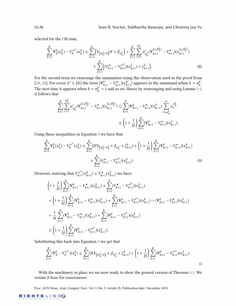
55:38 Sean R. Sinclair, Siddhartha Banerjee, and Christina Lee Yu
selected for the i’th time,
K’k=1
Vkh(x
kh ) V
k
h (xkh ) K’k=1
1[nk
h=0]H + nk
h
+
K’k=1
nkh’
i=1
inkh
(Vki (B
k
h)
h+1V?
h+1)(xki (B
k
h)
h+1)
+
K’k=1
(V?
h+1 V k
h+1)(xkh+1) +
kh+1
. (8)
For the second term we rearrange the summation using the observation used in the proof from[10, 25]. For every k 0 2 [K] the term (Vk 0
h+1V?
h+1)(xk
0
h+1) appears in the summand when k = nk
0
h.
The next time it appears when k = nk0
h+ 1 and so on. Hence by rearranging and using Lemma 3.1,
it follows that
K’k=1
nkh’
i=1
inkh
(Vki (B
k
h)
h+1V?
h+1)(xki (B
k
h)
h+1)
K’k=1
(Vkh+1 V
?
h+1)(xkh+1)
1’t=nk
h
nkh
t
1 +
1
H
K’k=1
(Vkh+1 V
?
h+1)(xkh+1).
Using these inequalities in Equation 8 we have that
K’k=1
Vkh(x
kh ) V
k
h (xkh ) K’k=1
(H1[nkh=0] + nk
h
+ kh+1) +
1 +
1
H
K’k=1
(Vkh+1 V
?
h+1)(xkh+1)
+
K’k=1
(V?
h+1 V k
h+1)(xkh+1). (9)
However, noticing that V k
h+1(xk
h+1) V?
h+1(xk
h+1) we have
1 +
1
H
K’k=1
(Vkh+1 V
?
h+1)(xkh+1) +
K’k=1
(V?
h+1 V k
h+1)(xkh+1)
=
1 +
1
H
K’k=1
(Vkh+1 V
?
h+1)(xkh+1) +
K’k=1
(Vkh+1 V
k
h+1)(xkh+1) (V
kh+1 V
?
h+1)(xkh+1)
=
1
H
K’k=1
(Vkh+1 V
?
h+1)(xkh+1) +
K’k=1
(Vkh+1 V
k
h+1)(xkh+1)
1 +
1
H
K’k=1
(Vkh+1 V
k
h+1)(xkh+1).
Substituting this back into Equation 9 we get that
K’k=1
(Vkh V
k
h )(xkh ) K’k=1
(H1[nkh=0] + nk
h
+ kh+1) +
1 +
1
H
K’k=1
(Vkh+1 V
k
h+1)(xkh+1).
With the machinery in place we are now ready to show the general version of Theorem 4.1. Werestate it here for convenience.
Proc. ACM Meas. Anal. Comput. Syst., Vol. 3, No. 3, Article 55. Publication date: December 2019.
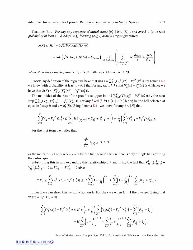
Adaptive Discretization for Episodic Reinforcement Learning in Metric Spaces 55:39
T E.12. For any any sequence of initial states xk1 | k 2 [K], and any 2 (0, 1) with
probability at least 1 Adaptive Q-learning (Alg 1) achieves regret guarantee:
R(K) 3H 2+ 6
p2H 3K log(4HK/ )
+ 96Hp
H 3 log(4HK/ ) + Ldmax
inf
r02(0,dmax ]
©≠≠≠’
r=dmax 2i
r r0
Nrdmax
r+
Kr0
dmax
™ÆÆÆ
where Nr is the r -covering number of S A with respect to the metric D.
P. By denition of the regret we have that R(K) =ÕK
k=1(V?
1 (xk1 )V k
1 (xk1 )). By Lemma E.8
we know with probability at least 1 /2 that for any (x ,a,h,k) that Vkh(x)V?
h(x) 0. Hence we
have that R(K) ÕKk=1(V
k1 (x
k1 ) V k
1 (xk1 )).
The main idea of the rest of the proof is to upper boundÕK
k=1(Vkh(xk
h) V k
h(xk
h)) by the next
stepÕK
k=1(Vkh+1
(xkh+1
) V k
h+1(xk
h+1)). For any xed (h,k) 2 [H ] [K] let Bk
hbe the ball selected at
episode k step h and t = nkh(B). Using Lemma E.11 we know for any h 2 [H ] that
K’k=1
(Vkh V
k
h )(xkh ) K’k=1
(H1[nkh=0] + nk
h
+ kh+1) +
1 +
1
H
K’k=1
(Vkh+1 V
k
h+1)(xkh+1).
For the rst term we notice that
K’k=1
1[nkh=0]H H
as the indicator is 1 only when k = 1 for the rst iteration when there is only a single ball coveringthe entire space.Substituting this in and expanding this relationship out and using the fact that Vk
H+1(xk
H+1)
V k
H+1(xk
h+1) = 0 as V k
H+1= V k
H+1= 0 gives
R(K) K’k=1
(V k1 (x
k1 ) V k
1 (xk1 )) H
H’h=1
1 +
1
H
h1+
H’h=1
1 +
1
H
h1 K’k=1
(nkh
+ kh+1).
Indeed, we can show this by induction on H . For the case when H = 1 then we get (using that
Vk2 (x) = V
k
2 (x) = 0)
K’k=1
(V k1 (x
k1 ) V k
1 (xk1 )) H +
1 +
1
H
K’k=1
Vk2 (x
k2 ) V k
2 (xk2 )+
K’k=1
nk1+ k2
= H
1’h=1
1 +
1
H
h1+
1’h=1
1 +
1
H
h1 K’k=1
nk1+ k2
.
Proc. ACM Meas. Anal. Comput. Syst., Vol. 3, No. 3, Article 55. Publication date: December 2019.
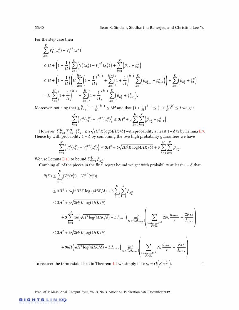
55:40 Sean R. Sinclair, Siddhartha Banerjee, and Christina Lee Yu
For the step case then
K’k=1
V k1 (x
k1 ) V k
1 (xk1 )
H +
1 +
1
H
K’k=1
Vk2 (x
k2 ) V k
2 (xk2 )+
K’k=1
nk1+ k2
H +
1 +
1
H
H
H1’h=1
1 +
1
H
h1+
H1’h=1
1 +
1
H
h1 K’k=1
nk
h+1+ kh+2
!+
K’k=1
nk1+ k2
= H
H’h=1
1 +
1
H
h1+
H’h=1
1 +
1
H
h1 K’k=1
nk
h
+ kh+1
.
Moreover, noticing thatÕHh=1
1 + 1
H
h1 3H and that1 + 1
H
h1 1 + 1
H
H 3 we get
K’k=1
V k1 (x
k1 ) V k
1 (xk1 ) 3H 2
+ 3
H’h=1
K’k=1
nk
h
+ kh+1
.
However,ÕK
k=1
ÕHh=1
kh+1 2
p2H 3K log(4HK/ )with probability at least 1/2 by Lemma E.9.
Hence by with probability 1 by combining the two high probability guarantees we have
K’k=1
V k1 (x
k1 ) V k
1 (xk1 ) 3H 2
+ 6p2H 3K log(4HK/ ) + 3
H’h=1
K’k=1
nkh
.
We use Lemma E.10 to boundÕK
k=1 nkh
.
Combing all of the pieces in the nal regret bound we get with probability at least 1 that
R(K) K’k=1
(V k1 (x
k1 ) V k
1 (xk1 ))
3H 2+ 6
q2H 3K log
4HK/
+ 3
H’h=1
K’k=1
nkh
3H 2+ 6
p2H 3K log(4HK/ )
+ 3
H’h=1
16p
H 3 log(4HK/ ) + Ldmax
inf
r02(0,dmax ]
©≠≠≠’
r=dmax 2i
r r0
2Nrdmax
r+
2Kr0
dmax
™ÆÆÆ 3H 2
+ 6p2H 3K log(4HK/ )
+ 96Hp
H 3 log(4HK/ ) + Ldmax
inf
r02(0,dmax ]
©≠≠≠’
r=dmax 2i
r r0
Nrdmax
r+
Kr0
dmax
™ÆÆÆTo recover the term established in Theorem 4.1 we simply take r0 = O
K
1dc +2
.
Proc. ACM Meas. Anal. Comput. Syst., Vol. 3, No. 3, Article 55. Publication date: December 2019.
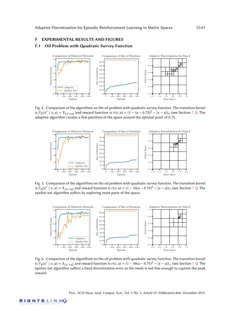
Adaptive Discretization for Episodic Reinforcement Learning in Metric Spaces 55:41
F EXPERIMENTAL RESULTS AND FIGURES
F.1 Oil Problem withadratic Survey Function
0 1000 2000 3000 4000 5000
Episode
0
1
2
3
4
5
ObservedReward
Comparison of Observed Rewards
Adaptive
Epsilon Net
0 1000 2000 3000 4000 5000
Episode
0
100
200
300
400
500
600
700
800
SizeofPartition
Comparison of Size of Partition
0.0 0.2 0.4 0.6 0.8 1.0
State Space
0.0
0.2
0.4
0.6
0.8
1.0
ActionSpace
Adaptive Discretization for Step 2
Fig. 4. Comparison of the algorithms on the oil problem with quadratic survey function. The transition kernel
is Ph (x0 | x ,a) = 1[x 0=a] and reward function is r (x ,a) = (1 (a 0.75)2 |x a |)+ (see Section 7.1). The
adaptive algorithm creates a fine partition of the space around the optimal point of 0.75.
0 1000 2000 3000 4000 5000
Episode
0
1
2
3
4
5
ObservedReward
Comparison of Observed Rewards
Adaptive
Epsilon Net
0 1000 2000 3000 4000 5000
Episode
0
100
200
300
400
500
600
700
800
SizeofPartition
Comparison of Size of Partition
0.0 0.2 0.4 0.6 0.8 1.0
State Space
0.0
0.2
0.4
0.6
0.8
1.0
ActionSpace
Adaptive Discretization for Step 2
Fig. 5. Comparison of the algorithms on the oil problem with quadratic survey function. The transition kernel
is Ph (x0 | x ,a) = 1[x 0=a] and reward function is r (x ,a) = (1 10(a 0.75)2 |x a |)+ (see Section 7.1). The
epsilon net algorithm suers by exploring more parts of the space.
0 1000 2000 3000 4000 5000
Episode
0
1
2
3
4
5
ObservedReward
Comparison of Observed Rewards
Adaptive
Epsilon Net
0 1000 2000 3000 4000 5000
Episode
0
100
200
300
400
500
600
700
800
SizeofPartition
Comparison of Size of Partition
0.0 0.2 0.4 0.6 0.8 1.0
State Space
0.0
0.2
0.4
0.6
0.8
1.0
ActionSpace
Adaptive Discretization for Step 2
Fig. 6. Comparison of the algorithms on the oil problem with quadratic survey function. The transition kernel
is Ph (x0 | x ,a) = 1[x 0=a] and reward function is r (x ,a) = (1 50(a 0.75)2 |x a |)+ (see Section 7.1). The
epsilon net algorithm suers a fixed discretization error as the mesh is not fine enough to capture the peak
reward.
Proc. ACM Meas. Anal. Comput. Syst., Vol. 3, No. 3, Article 55. Publication date: December 2019.
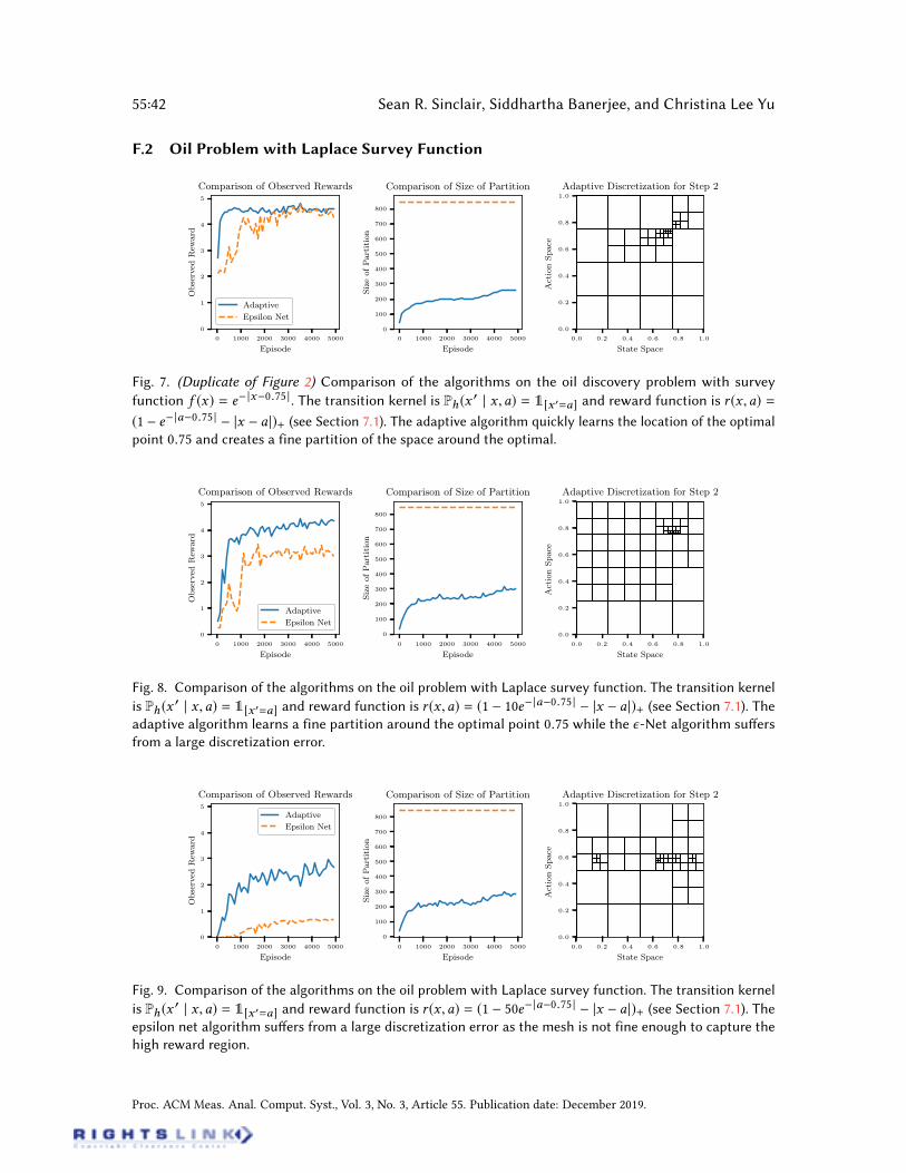
55:42 Sean R. Sinclair, Siddhartha Banerjee, and Christina Lee Yu
F.2 Oil Problem with Laplace Survey Function
0 1000 2000 3000 4000 5000
Episode
0
1
2
3
4
5
ObservedReward
Comparison of Observed Rewards
Adaptive
Epsilon Net
0 1000 2000 3000 4000 5000
Episode
0
100
200
300
400
500
600
700
800
SizeofPartition
Comparison of Size of Partition
0.0 0.2 0.4 0.6 0.8 1.0
State Space
0.0
0.2
0.4
0.6
0.8
1.0
ActionSpace
Adaptive Discretization for Step 2
Fig. 7. (Duplicate of Figure 2) Comparison of the algorithms on the oil discovery problem with survey
function f (x) = e |x0.75 | . The transition kernel is Ph (x0 | x ,a) = 1[x 0=a] and reward function is r (x ,a) =
(1 e |a0.75 | |x a |)+ (see Section 7.1). The adaptive algorithm quickly learns the location of the optimal
point 0.75 and creates a fine partition of the space around the optimal.
0 1000 2000 3000 4000 5000
Episode
0
1
2
3
4
5
ObservedReward
Comparison of Observed Rewards
Adaptive
Epsilon Net
0 1000 2000 3000 4000 5000
Episode
0
100
200
300
400
500
600
700
800
SizeofPartition
Comparison of Size of Partition
0.0 0.2 0.4 0.6 0.8 1.0
State Space
0.0
0.2
0.4
0.6
0.8
1.0
ActionSpace
Adaptive Discretization for Step 2
Fig. 8. Comparison of the algorithms on the oil problem with Laplace survey function. The transition kernel
is Ph (x0 | x ,a) = 1[x 0=a] and reward function is r (x ,a) = (1 10e |a0.75 | |x a |)+ (see Section 7.1). The
adaptive algorithm learns a fine partition around the optimal point 0.75 while the -Net algorithm suers
from a large discretization error.
0 1000 2000 3000 4000 5000
Episode
0
1
2
3
4
5
ObservedReward
Comparison of Observed Rewards
Adaptive
Epsilon Net
0 1000 2000 3000 4000 5000
Episode
0
100
200
300
400
500
600
700
800
SizeofPartition
Comparison of Size of Partition
0.0 0.2 0.4 0.6 0.8 1.0
State Space
0.0
0.2
0.4
0.6
0.8
1.0
ActionSpace
Adaptive Discretization for Step 2
Fig. 9. Comparison of the algorithms on the oil problem with Laplace survey function. The transition kernel
is Ph (x0 | x ,a) = 1[x 0=a] and reward function is r (x ,a) = (1 50e |a0.75 | |x a |)+ (see Section 7.1). The
epsilon net algorithm suers from a large discretization error as the mesh is not fine enough to capture the
high reward region.
Proc. ACM Meas. Anal. Comput. Syst., Vol. 3, No. 3, Article 55. Publication date: December 2019.
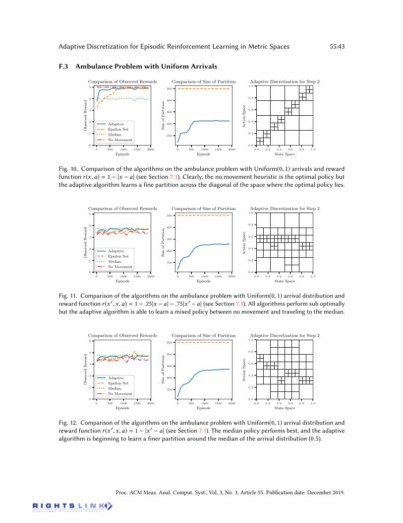
Adaptive Discretization for Episodic Reinforcement Learning in Metric Spaces 55:43
F.3 Ambulance Problem with Uniform Arrivals
0 500 1000 1500 2000
Episode
0
1
2
3
4
5ObservedReward
Comparison of Observed Rewards
Adaptive
Epsilon Net
Median
No Movement
0 500 1000 1500 2000
Episode
100
200
300
400
500
SizeofPartition
Comparison of Size of Partition
0.0 0.2 0.4 0.6 0.8 1.0
State Space
0.0
0.2
0.4
0.6
0.8
1.0
ActionSpace
Adaptive Discretization for Step 2
Fig. 10. Comparison of the algorithms on the ambulance problem with Uniform(0, 1) arrivals and reward
function r (x ,a) = 1 |x a | (see Section 7.1). Clearly, the no movement heuristic is the optimal policy but
the adaptive algorithm learns a fine partition across the diagonal of the space where the optimal policy lies.
0 500 1000 1500 2000
Episode
0
1
2
3
4
5
ObservedReward
Comparison of Observed Rewards
Adaptive
Epsilon Net
Median
No Movement
0 500 1000 1500 2000
Episode
100
200
300
400
500
SizeofPartition
Comparison of Size of Partition
0.0 0.2 0.4 0.6 0.8 1.0
State Space
0.0
0.2
0.4
0.6
0.8
1.0
ActionSpace
Adaptive Discretization for Step 2
Fig. 11. Comparison of the algorithms on the ambulance problem with Uniform(0, 1) arrival distribution and
reward function r (x 0,x ,a) = 1 .25|x a | .75|x 0 a | (see Section 7.1). All algorithms perform sub optimally
but the adaptive algorithm is able to learn a mixed policy between no movement and traveling to the median.
0 500 1000 1500 2000
Episode
0
1
2
3
4
5
ObservedReward
Comparison of Observed Rewards
Adaptive
Epsilon Net
Median
No Movement
0 500 1000 1500 2000
Episode
100
200
300
400
500
SizeofPartition
Comparison of Size of Partition
0.0 0.2 0.4 0.6 0.8 1.0
State Space
0.0
0.2
0.4
0.6
0.8
1.0
ActionSpace
Adaptive Discretization for Step 2
Fig. 12. Comparison of the algorithms on the ambulance problem with Uniform(0, 1) arrival distribution and
reward function r (x 0,x ,a) = 1 |x 0 a | (see Section 7.1). The median policy performs best, and the adaptive
algorithm is beginning to learn a finer partition around the median of the arrival distribution (0.5).
Proc. ACM Meas. Anal. Comput. Syst., Vol. 3, No. 3, Article 55. Publication date: December 2019.
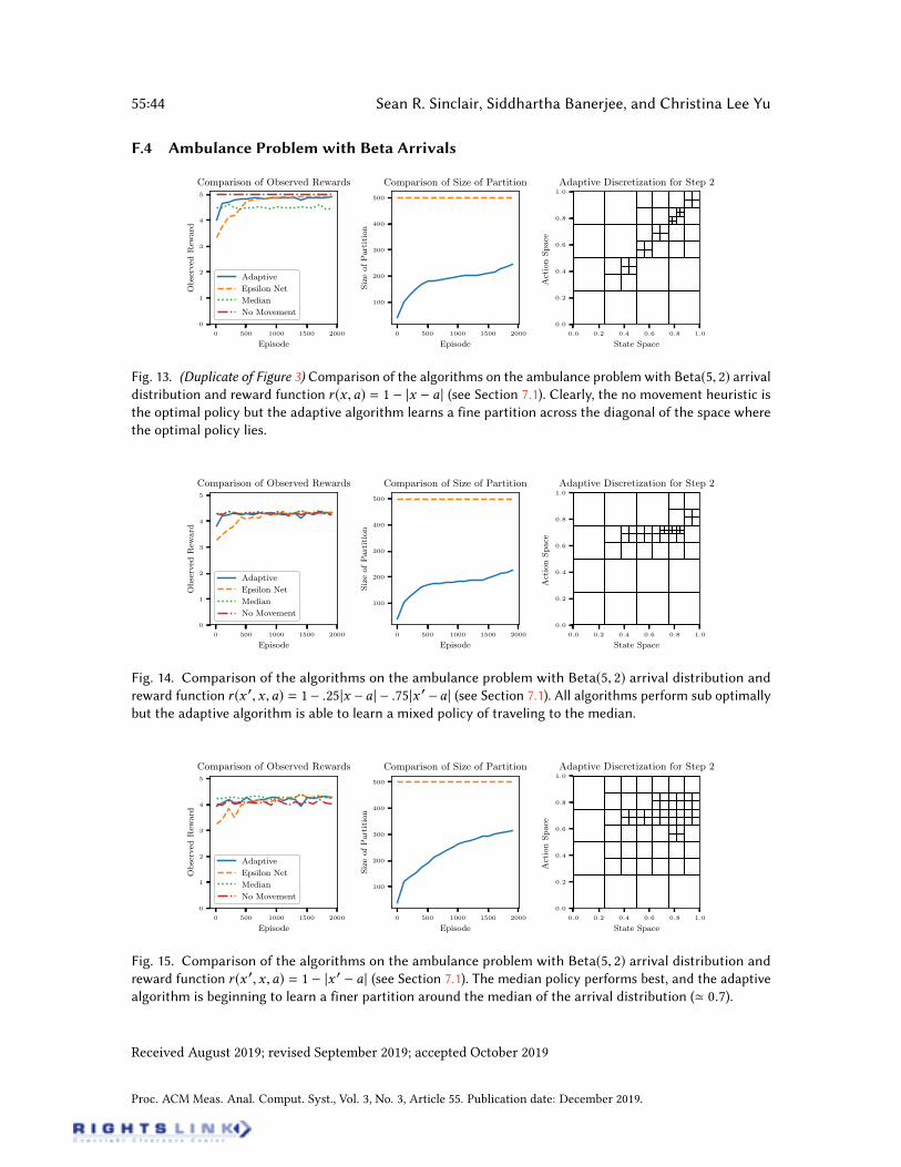
55:44 Sean R. Sinclair, Siddhartha Banerjee, and Christina Lee Yu
F.4 Ambulance Problem with Beta Arrivals
0 500 1000 1500 2000
Episode
0
1
2
3
4
5ObservedReward
Comparison of Observed Rewards
Adaptive
Epsilon Net
Median
No Movement
0 500 1000 1500 2000
Episode
100
200
300
400
500
SizeofPartition
Comparison of Size of Partition
0.0 0.2 0.4 0.6 0.8 1.0
State Space
0.0
0.2
0.4
0.6
0.8
1.0
ActionSpace
Adaptive Discretization for Step 2
Fig. 13. (Duplicate of Figure 3) Comparison of the algorithms on the ambulance problem with Beta(5, 2) arrival
distribution and reward function r (x ,a) = 1 |x a | (see Section 7.1). Clearly, the no movement heuristic is
the optimal policy but the adaptive algorithm learns a fine partition across the diagonal of the space where
the optimal policy lies.
0 500 1000 1500 2000
Episode
0
1
2
3
4
5
ObservedReward
Comparison of Observed Rewards
Adaptive
Epsilon Net
Median
No Movement
0 500 1000 1500 2000
Episode
100
200
300
400
500
SizeofPartition
Comparison of Size of Partition
0.0 0.2 0.4 0.6 0.8 1.0
State Space
0.0
0.2
0.4
0.6
0.8
1.0
ActionSpace
Adaptive Discretization for Step 2
Fig. 14. Comparison of the algorithms on the ambulance problem with Beta(5, 2) arrival distribution and
reward function r (x 0,x ,a) = 1 .25|x a | .75|x 0 a | (see Section 7.1). All algorithms perform sub optimally
but the adaptive algorithm is able to learn a mixed policy of traveling to the median.
0 500 1000 1500 2000
Episode
0
1
2
3
4
5
ObservedReward
Comparison of Observed Rewards
Adaptive
Epsilon Net
Median
No Movement
0 500 1000 1500 2000
Episode
100
200
300
400
500
SizeofPartition
Comparison of Size of Partition
0.0 0.2 0.4 0.6 0.8 1.0
State Space
0.0
0.2
0.4
0.6
0.8
1.0
ActionSpace
Adaptive Discretization for Step 2
Fig. 15. Comparison of the algorithms on the ambulance problem with Beta(5, 2) arrival distribution and
reward function r (x 0,x ,a) = 1 |x 0 a | (see Section 7.1). The median policy performs best, and the adaptive
algorithm is beginning to learn a finer partition around the median of the arrival distribution (' 0.7).
Received August 2019; revised September 2019; accepted October 2019
Proc. ACM Meas. Anal. Comput. Syst., Vol. 3, No. 3, Article 55. Publication date: December 2019.