local discretization error bounds using interval boundary element method

INTERNATIONAL JOURNAL FOR NUMERICAL METHODS IN ENGINEERINGInt. J. Numer. Meth. Engng 2009; 78:403–428Published online 12 November 2008 in Wiley InterScience (www.interscience.wiley.com). DOI: 10.1002/nme.2490

Local discretization error bounds using interval boundaryelement method

B. F. Zalewski∗,† and R. L. Mullen

Department of Civil Engineering, Case Western Reserve University, 10900 Euclid Avenue,Cleveland, OH 44106, U.S.A.

SUMMARY

In this paper, a method to account for the point-wise discretization error in the solution for boundaryelement method is developed. Interval methods are used to enclose the boundary integral equation and asharp parametric solver for the interval linear system of equations is presented. The developed method doesnot assume any special properties besides the Laplace equation being a linear elliptic partial differentialequation whose Green’s function for an isotropic media is known. Numerical results are presented showingthe guarantee of the bounds on the solution as well as the convergence of the discretization error. Copyrightq 2008 John Wiley & Sons, Ltd.

Received 4 April 2008; Revised 6 August 2008; Accepted 22 September 2008

KEY WORDS: boundary element method; interval boundary element method; local discretization error;parametric interval solver

1. INTRODUCTION

The behavior of most engineering systems is governed by partial differential equations. In general,the exact solution to those equations cannot be found due to the difficulties associated with satisfyinga correct set of boundary conditions for any geometry of the system. Numerical methods, suchas finite element method (FEM), finite difference method, and boundary element method (BEM),have been developed to obtain approximate discrete solutions to partial differential equations.These methods require that only a finite number of discrete solutions be considered to obtain alinear system of equations resulting in discretization error. Although a solution at any point in thesystem can be obtained using the computed discrete values and the weighted residual functions,the solution at that point is not exact due to the discretization error present in the computed discretevalues. If these solutions were exact, an exact solution at any point could be computed.

∗Correspondence to: B. F. Zalewski, Department of Civil Engineering, Case Western Reserve University, 10900Euclid Avenue, Cleveland, OH 44106, U.S.A.

†E-mail: [email protected]

Contract/grant sponsor: Center for Reliable Engineering Computing (REC)

Copyright q 2008 John Wiley & Sons, Ltd.

404 B. F. ZALEWSKI AND R. L. MULLEN

For some engineering systems, experimental techniques can be used to validate the numericalsimulations. However, those experiments become very expensive for larger systems. Thus, thevalidity of point-wise solutions obtained from numerical simulations for any system cannot beverified by conventional methods. Moreover, reliable engineering computing is affected by theuncertainties in the parameters describing the physical system, uncertainties in the applied boundaryconditions, errors resulting from numerical integration, and errors resulting from floating pointtruncation. Uncertainty in the parameters of the system has been treated using a possibilisticapproach with fuzzy sets [1], evidence theory [2, 3], and interval approach [4–8]. Interval finiteelement method [4–6] has been developed to address the uncertainty in system’s parameters,boundary conditions, and truncation error [8–17]. Global discretization error has been shownto converge monotonically for FEM [18, 19]; however, the impact of the discretization on thepoint-wise values has not been explored.

BEM is an alternate technique used to approximate solutions to partial differential equations.The method uses fundamental solutions, or Green’s functions, to partial differential equations toreduce the dimension of the weak form. This dimension reduction technique allows for a fastermesh generation or a faster mesh refinement compared with FEM making it easier to investigatedifferent design options. In order to obtain residual only on the boundary of the system, andtherefore to reduce the dimension of the weak form, the boundary integral equations are solvedusing point collocation methods. In the point collocation method the residual is set to zero in thedomain of the problem and nonzero on the boundary of the domain. The resulting weak form isintegrated such that all variables are transformed to the boundary of the domain.

Uncertainties in BEM solutions can be attributed to uncertainty in the applied boundary condi-tions, uncertainty in the system parameters, integration errors, truncation errors, and discretizationerrors. Interval boundary element method (IBEM) [20] has been developed to account for theuncertainty in boundary conditions, integration error, and truncation error. Global discretizationerror in the integral equations for solutions to harmonic and bi-harmonic problems [21] and forBEM [22, 23] was shown to converge.

This paper discusses the interval treatment of local discretization error in IBEM illustratedon a torsion problem. The integral boundary equations resulting from the boundary elementformulation are bounded using the interval kernel splitting technique (IKST), which is consistentwith the boundary element formulation. In this work, the applied boundary condition functions areconsidered as exact and are treated on the boundary integral equation level. A parametric solverfor the interval linear system of equations is developed resulting in guaranteed bounds for thesolution. Numerical solutions to the torsion problem of a rectangular cross section are presented todemonstrate the convergence of the local discretization error and to show the stability of the erroroverestimation with problem size. The effect of the parameterization on the convergence of thesolution bounds and on the computational time is studied. A second example obtains the boundson the local discretization error of the fluxes for an L-shaped domain, where a potential satisfiesthe Laplace equation, and demonstrates the convergence of the interval solutions.

2. BOUNDARY ELEMENT ANALYSIS OF THE LAPLACE EQUATION

The following section reviews the boundary element formulation for the Laplace equation [24, 25]in two dimensions. There is no loss in generality in the formulation as a similar procedure can be

Copyright q 2008 John Wiley & Sons, Ltd. Int. J. Numer. Meth. Engng 2009; 78:403–428DOI: 10.1002/nme

LOCAL DISCRETIZATION ERROR IN BOUNDARY ELEMENT METHOD 405

used for any linear elliptic partial differential equation. The Laplace equation is

∇2u = 0 in �

u = u on �1

�u�n

= q= q on �2

(1)

where � is the domain of the system, �1 and �2 are the boundaries of the system such that�1∪�2=� and �1∩�2=0, u is the potential with a Dirichlet boundary condition u on boundary�1, q is the flux with a Neumann boundary condition of q on boundary �2, and n is the outwardnormal vector. In order to solve Equation (1) by approximate methods, Equation (1) is firstexpressed in a weighted residual form∫

�∇2uwd�=

∫�2

(q− q)wd�2−∫

�1

(u− u)�w

�nd�1 (2)

where function w is the weighted residual function. The left-hand side of Equation (2) is integratedby parts twice to reduce the smoothness requirements on the solution. This is an essential step inthe boundary element formulation in order to decrease the dimension of the approximation. Theresult is a nonsymmetric weak form that has weaker smoothness requirements than the weak formused in finite element formulation. After integration by parts is performed twice, the boundaryterms are collected together on �1 and �2, allowing Equation (2) to be rewritten as:∫

�∇2wu d�=−

∫�2

qwd�2−∫

�1

qwd�1+∫

�2

u�w

�nd�2+

∫�1

u�w

�nd�1 (3)

In order for Equation (3) to consist of integral terms on the boundary of the domain only, theleft-hand side integral over the domain must be addressed. The procedure that is used to obtain theintegral terms only on the boundary of the domain is the point collocation method. In this method,the residual is set to zero in the domain and nonzero only on the boundary of the domain. This isexpressed by considering the weighted residual function w that satisfies

∇2w=−�(x−�) (4)

where � is the source point or a point at which a concentrated charge acts, x is the field pointat which the response of the concentrated charge is considered, and �(x−�) is the Dirac deltafunction having the properties: ∫

��(x)d� = 1 (5)

∫�

�(x−�) f (x)d� = f (�) (6)

The solution to Equation (4) is called the fundamental solution, or Green’s function, of the partialdifferential equation and is denoted by u∗. Since the point collocation method is used to reduce thedimension of Equation (3), the boundary element formulation can be performed only for the partialdifferential equations whose Green’s function is known. For Laplace equation, the fundamentalsolution for an isotropic media is known and used throughout the paper to illustrate the boundary



element formulation. It should be noted that no special properties of the Laplace equation areconsidered in the development of the boundary element formulation, and the same procedure canbe performed for any linear elliptic partial differential equation whose fundamental solution isknown. For a two-dimensional isotropic media, the solution to Equation (4) is given as

u∗ = − 1

2�ln(r) (7)

q∗ = − 1

2�r2(x−�) ·n (8)

where r =|x−�| is the distance between the source point � and any point of interest x . Lettingw=u∗ and q∗ =�u∗/�n result in Equation (3) to be rewritten as:∫

�∇2u∗u d�=−

∫�2

qu∗ d�2−∫

�1

qu∗ d�1+∫

�2

uq∗ d�2+∫

�1

uq∗ d�1 (9)

Substituting Equation (4) into Equation (9) yields:

u(�)+∫

�2

q∗(x,�)u(x)dx+∫

�1

q∗(x,�)u(x)dx

=∫

�1

u∗(x,�)q(x)dx+∫

�2

u∗(x,�)q(x)dx, �∈� (10)

Considering a mixed boundary problem, Equation (10) can be rewritten as:

u(�)+∫

�q∗(x,�)u(x)dx=

∫�u∗(x,�)q(x)dx, �∈� (11)

Although Equation (11) contains all integral terms over the boundary of the domain, the sourcepoint � is included in the domain. Hence, Equation (11) is integrated such that the source point �is enclosed by a circular boundary of radius ε as ε→0 (Figure 1). Substituting Equation (7) intoEquation (11) allows the right-hand side integral to vanish as:

limε→0

∫�

− 1

2�ln(r)q d�= lim

ε→0

∫ �

�=0− 1

2�ln(ε)qεd�=− 1

2�limε→0

∫ �

�=0

ln(ε)q

1/εd�=0 (12)

Figure 1. Reduction of the dimension of approximation in boundary element formulation.



By substituting Equation (8) into Equation (11), the left-hand side integral is evaluated as

limε→0

∫�

− u

2�r2(x−�) ·n d�= lim

ε→0

∫ �

�=0− uε

2�ε2εd�=− 1

2�limε→0

∫ �

�=0u d�=− �

2�u (13)

where � is an angle on the boundary of the domain with a value of �=� for smooth boundaries.Equation (11) can be thus rewritten such that it consists of only the terms on the boundary of thedomain as:

1

2u(�)+

∫�q∗(x,�)u(x)dx=

∫�u∗(x,�)q(x)dx, �∈� (14)

The weak form, which is entirely composed of terms on the boundary of the system, such asEquation (14), is the staring point for the boundary element formulation. Discretizing the integralsof Equation (14) over n sub-domains can be performed resulting in

1

2u(�)+

n∑k=1

∫�k

q∗(x,�)u(x)dx=n∑

k=1

∫�k

u∗(x,�)q(x)dx, �∈� (15)

where⋃n

k=1�k =� and⋂n

k=1�k =0. It should be noted that Equation (15) is solved exactly forall the values of � on the boundary of the system and therefore no approximation is performedas of yet. Equation (15) is discretized by considering a finite number of source points at which avalue of either u or q is known. The functions u(x) and q(x) are also approximated as

u(x) = �(x)ui (16)

q(x) = �(x)qi (17)

where ui and qi are the vectors of nodal values of u and q , respectively, at node i , and �(x) isthe vector of interpolation functions. The discretized boundary integral equation is written as:

1

2ui +

n∑k=1

∫�k

q∗(x,�)�(x)dxui =n∑

k=1

∫�k

u∗(x,�)�(x)dxqi (18)

Equation (18) can be solved exactly if all the locations of the source points on the boundary of thesystem were considered. The preceding procedure, Equations (15)–(18), can also be expressed interms of boundary elements instead of boundary integral equations. Boundary � is approximatedby boundary elements �i consisting of nodes at which a value of either u or q is known withassumed polynomial interpolation functions between nodes as:

1

2ui + ∑

Elements

∫�q∗(x,�)�(x)dxui = ∑

Elements

∫�u∗(x,�)�(x)dxqi (19)

As Equations (15), (19) can be exactly solved if all locations of the source points are consid-ered on each element. In this work, constant boundary elements are used to generate significantdiscretization errors. Higher-order elements are assumed to better approximate the true solutionand therefore have smaller discretization errors. The methodology presented in this paper is notlimited by the use of constant elements, which are used mainly to illustrate the procedure, and itcan be readily extended to higher-order approximation. Constant elements contain one node per



element, leading to the following discretization:

u(x) = �ui (20)

q(x) = �qi (21)

where ui and qi are the vectors of nodal values of u and q , respectively, at node i , and � is thevector of constant interpolation functions. The discretized boundary integral equation with constantboundary elements is written as:

1

2ui + ∑

Elements

∫�q∗(x,�)�dxui = ∑

Elements

∫�u∗(x,�)�dxqi (22)

The interpolation function must be equal to one at the node, and therefore Equation (22) can berewritten as:

1

2ui + ∑

Elements

∫�q∗(x,�)dxui = ∑

Elements

∫�u∗(x,�)dxqi (23)

Equation (23) can be written in a matrix form as

Hu=Gq (24)

where matrix H is singular. Equation (24) is rearranged according to the boundary conditions andsolved as a linear algebra problem:

Ax=b (25)

The described boundary element formulation is performed for a torsion problem expressed in termsof the Laplace equation.

3. TORSION OF A RECTANGULAR BAR

The following section reviews the torsion problem for a rectangular bar with horizontal sides oflength of 2a and the vertical sides of length 2b [26] (Figure 2). The torsion problem is expressedin terms of the Laplace operator on the warping function � as

∇2�=0 in � (26)

with the Neumann boundary condition satisfied as:(��

�x1−x2

)dx2ds

−(

��

�x2+x1

)dx1ds

=0 on � (27)

On the sides of the rectangle, the Neumann boundary conditions are:

��

�x1= ��

�n1

�n1�x1

= x2, x1=a (28)

��

�x1= ��

�n1

�n1�x1

=−x2, x1=−a (29)



��

�x2= ��

�n2

�n2�x2

=−x1, x2=b (30)

��

�x2= ��

�n2

�n2�x2

= x1, x2=−b (31)

To simplify the boundary conditions, a modified warping function �1 is defined as:

�1= x1x2−� (32)

The problem is rewritten in terms of the Laplace equation as:

∇2�1=0 in � (33)

The boundary conditions for the edges are then defined as:

��1

�n1= 0 on x1=±a (34)

��1

�n2= 2x1 on x2=±b (35)

Applying the chain rule to Equations (34) and (35) results in the boundary conditions as (Figure 3):

��1

�x1= 0 on x1=±a (36)

��1

�x2= 2x1 on x2=b (37)

��1

�x2= −2x1 on x2=−b (38)

Figure 2. Cross section of a rectangular beam.



Figure 3. Neumann boundary conditions for a torsion of a rectangular beam.

The true solution for the modified warping function �1 can be obtained as an infinite series andis given [26] as

�1 = 32a2

�3∞∑n=0

(−1)n sin(knx1)sinh(knx2)

(2n+1)3 cosh(knb)(39)

kn = (2n+1)�

2a(40)

where x1 and x2 are the coordinates (Figure 2), and a and b are half of the lengths of the sides ofthe rectangular cross section (Figure 2). The solution to the warping function � can be obtainedfrom Equations (32) and (39) as:

�= x1x2− 32a2

�3∞∑n=0

(−1)n sin(knx1)sinh(knx2)

(2n+1)3 cosh(knb)(41)

The torsion problem cannot be generally solved exactly due to the complications in the geometryof the cross section and the complicated boundary conditions. Thus, numerical methods are used toobtain approximate solutions to the torsion problem. In this work BEM is used in the computations.

4. BOUNDARY CONDITIONS FOR CONSTANT BOUNDARY ELEMENTS

The torsion problem consists of complicated boundary conditions, which cannot be exactly eval-uated using constant boundary elements. The treatment of those boundary conditions on theintegral boundary equation level is described in this section. The torsion problem is subjected tofunctional boundary conditions, Equations (34) and (35), which cannot be correctly modeled byconstant boundary elements. The constant boundary element formulation, Equation (23), requires



that the interpolation functions be in the H0 Hilbert space and the given boundary conditions are inhigher-order Hilbert space. However, the part of the boundary integral equation, Equation (15), atwhich the boundary conditions are given, can be evaluated explicitly since both the kernel and theboundary condition function are known. In this study boundary conditions are computed explicitlyfrom boundary integral equations. This procedure is performed since the boundary conditions areexplicitly known and treating them as uncertain [20] will result in bounds which enclose boundaryconditions that do not correspond to the torsion problem.

5. INTERVAL ANALYSIS

In this work, the discretization error in BEM is treated using an interval approach. The followingis a review of interval analysis [7, 8]. In this paper interval quantities are represented by a boldletter, such as an interval number x and an interval-valued function f(x). For an interval numberx=[x, x], x denotes the lower bound and x denotes the upper bound. An interval number x=[a,b]is a set of real numbers such that

[a,b]={x |a�x�b} (42)

where (a,b)∈. Interval variables x=[a,b] and y=[c,d] behave according to the followingoperations:Addition:

x+y=[a+c,b+d] (43)

Subtraction:

x−y=[a−d,b−c] (44)

Multiplication:

x ·y=[min{ac,ad,bc,bd},max{ac,ad,bc,bd}] (45)

Division:

xy

=[a,b]·[1

d,1

c

], 0 /∈y (46)

Integration of interval-valued function f(x,n), which is a class of all possible functions boundedby a given interval, is performed as:∫

�f(x,n)d�=

[∫�f (x,�)d�,

∫�f (x,�)d�

], �∈[�, �] (47)

Subdistributive property:

x ·(y+z)⊆x ·y+x ·z (48)

One of the major sources of overestimation or underestimation in interval solutions is the incorrector naıve usage subdistributive property of interval numbers. Great emphasis should be made tothe correct order of operations in interval analysis. If the correct representation is given by the left



term in Equation (48), expressing the operation by the right term may cause overestimation. If thecorrect representation is expressed as the right term in Equation (48), expressing it as the left termmay result in inner bounds and the enclosure of the solution may not be guaranteed. This issuewill be further referred to in considering interval kernel functions.

Another source of overestimation occurs due to the dependency of interval numbers, eitherlinear or non-linear. Linear dependency of interval numbers for x=[−1,1] and y=[−1,1] can beillustrated as:

x ·y= [−1,1] (49)

x ·x= [0,1] (50)

Equation (49) considers two independent sets, whereas Equation (50) considers every numberin set x to be multiplied by itself. For engineering problems the interval dependency, linear ornon-linear, occurs mostly due to the physics of the problem and needs to be considered for sharpsolutions. Naive interval application may results in wide and unrealistic bounds. Considering theexample to illustrate non-linear interval dependency

y=6 ·x ·x+3 ·x, x=[−1,1]results in naive bounds for the solution, y=[−9,9] if direct interval implementation is performed.However, considering interval dependency, the bounds on the solution result in exact bounds,y=[−0.375,9]. Another source of overestimation is the order of operations in interval linearalgebra [4, 5]. To obtain sharp results, interval operations should be performed last to reducethe overestimation due to the dependency in interval matrix coefficients. The following exampledemonstrates this consideration:

y1 = A ·(B ·x), y2=(A ·B) ·x

A =[a11 a12

a21 a22

], B=

[b11 b12

b21 b22

], x=

[x1

x2

]

y1 =[a11(b11x1+b12x2)+a12(b21x1+b22x2)

a21(b11x1+b12x2)+a22(b21x1+b22x2)

]

y2 =[

(a11b11+a12b21)x1+(a11b12+a12b22)x2

(a21b11+a22b21)x1+(a21b12+a22b22)x2

]

It can be clearly seen that y2 is sharper than y1 due to considered dependency of x1 and x2throughout the rows of y2, and therefore special care should be given to the order of intervaloperations to obtain sharp bounds on the solution.

6. INTERVAL BOUNDARY ELEMENT METHOD

IBEM has been developed to address the impact of the uncertainty in boundary conditions, integra-tion error, and truncation error on the solutions [20]. The IBEM formulation results in the interval



linear system of equations

Hu=Gq (51)

which is rearranged according to the boundary conditions yielding:

Ax=b (52)

The treatment of the discetization error in IBEM is described in the latter sections. The iterativesolution to Equation (52) is described in the following section.

7. INTERVAL LINEAR SYSTEM OF EQUATIONS

The interval linear system of equations (52) is solved using Krawczyk iteration [27] based onBrouwer’s fixed point theorem [4–6]. One approach of self-validating methods to find the zero ofthe function f (x)=0, n →n is to consider a fixed point function g(x)= x . The transformationbetween f (x) and g(x) for a nonsingular preconditioning matrix C is

f (x) = 0⇔g(x)= x (53)

g(x) = x−C · f (x) (54)

where the function g(x) is considered as a Newton operator. From Brouwer’s fixed point theoremand from

g(x)⊆x for some x∈n (55)

the following is true:

∃ x ∈x : f (x)=0 (56)

This method is used to solve the linear system of equations (52). The preconditioning matrix C ischosen as C= A−1. From Equations (54) and (55) it follows that:

Cb+(I −CA)x⊆x (57)

The left-hand side of Equation (57) is the Krawczyk operator [27]. For the iteration to providefinite solution, the preconditioning matrix needs to be proven regular [8, 16]. The following provesthis condition.

Theorem 1 (Rump [16])Let A, C ∈n×n , b∈n , and x∈n be given. If

Cb+(I −CA)x⊆ int(x) (58)

then C and A are regular and the unique solution of Ax=b satisfies A−1b∈x. int(x) refers to theinterior of x. However, all terms in Equation (52) are interval terms, thus the following is a prooffor the guarantee of the solution for the equation of this form.



Theorem 2 (Rump [16])Let A∈n×n , C ∈n×n , b∈n , and x∈n be given. If

Cb+(I −CA)x⊆ int(x) (59)

then C and every matrix A∈A is regular and∑(A,b)={x ∈n|∃ A∈A∃b∈b : Ax=b}⊆x (60)

Equation (60) guarantees the solution to the interval linear system of equations (52). The residualform of Equation (60) is [8]

Cb−CAx0+(I −CA)d⊆ int(d) (61)

where x= x0+d. A good initial guess is x0=Cmidb, where C=midA−1.

8. DISCRETIZATION ERROR IN BEM

The discretization error in the solutions to the integral equations results from considering a finitenumber of points for which the solutions are computed. In general, the true solutions to integralequations are functions, not discrete values, and therefore the space of the approximate solutionsdoes not cover the space of the true solutions. The boundary integral equations can be obtainedby the use of collocation methods resulting in equation of the form of (14). The boundary integralequations are satisfied exactly only if all the locations of the source point � on the boundary areconsidered. However, to obtain a linear system of equations, a finite amount of source points isconsidered. Moreover, the location of the source points is unique and the solution is considered asa polynomial interpolation between the discrete values whose location corresponds to the locationof the source point. This allows for the linear system of equations to be unique and thus thesystem can be solved for the unknown boundary values. It should be noted that if all sourcepoints are considered, the boundary values at all points can be computed, resulting in the truesolution. The boundary integral equation can also be evaluated over n sub-domains as expressedby Equation (15). The unique location of the source point and its correspondence to the point atwhich the approximate solution is computed must be satisfied for all sub-domains. Equation (15) issatisfied exactly only if all the locations of the source point are considered. Thus, the discretizationerror is introduced in the same manner as in Equation (14).

In the analysis of the discretization error, all the locations of the source point in the continuousboundary integral equation, Equation (14), are treated via interval approach. Considering intervalbounds on all the possible locations of the source points allow to obtain interval solutions, whichenclose the true solution. From the interval bounds on the boundary values, the bounds on thetrue solution for any point in the domain can be computed. Equation (14) is enclosed by aninterval boundary integral equation in which the terms u∗(x,�) and q∗(x,�) are enclosed by knowninterval-valued functions. The unknown functions u(x) and q(x) in Equation (14) are then boundedby interval values enclosing the true solution.

In this paper the following problem statement of enclosing discretization error is defined interms of interval Gauss–Seidel iteration due to the natural correspondence of the problem to thistype of iteration. The integral over the domain can be expressed as the sum of the integrals over theelements, Equation (19), and thus the boundary integral equation must be enclosed on each element



Figure 4. Interval bounds on a solution over an element.

for all the locations of the source points. Hence, for the boundary � subdivided into n boundaryelements, for each element j the interval values u or q that bound the functions u(x) or q(x) arefound (Figure 4). It is assumed that on all other elements except for the element in considerationthe bounds on all boundary values are known. In addition, either the Dirichlet or the Neumannboundary condition bounds are known for the element in consideration and the remaining boundaryvalue for the single element in consideration is enclosed. The process is repeated for the secondelement with the assumed bounds for all the other elements, a computed bound for the previouslyconsidered element, and either the Dirichlet or the Neumann boundary condition bounds for thesecond element in consideration. The procedure known as the interval Gauss–Seidel iteration [8]can be performed for all elements until the true solution is enclosed. Mathematically, the abovestatement can be expressed as:

∀ j ∈{1,2, . . . ,n} Assume ui�ui�ui , qi�qi�qi is known ∀i �= j . Also known q j�q j�q j . Findu j�u j�u j

∀� j

∣∣∣∣∣∣∣∣∣

1

2u(� j )+

∫� j

q∗(x,� j )u j (x)d� j =n∑

i=1i �= j

∫�i

u∗(x,� j )qi (x)d�i

+∫

� j

u∗(x,� j )q j (x)d� j −n∑

i=1i �= j

∫�i

q∗(x,� j )ui (x)d�i

Or∀ j ∈{1,2, . . . ,n} Assume ui�ui�ui , qi�qi�qi is known ∀i �= j . Also known u j�u j�u j . Find

q j�q j�q j

∀� j

∣∣∣∣∣∣∣∣∣

∫� j

u∗(x,� j )q j (x)d� j = 1

2u(� j )+

∫� j

q∗(x,� j )u j (x)d� j

+n∑

i=1i �= j

∫�i

q∗(x,� j )ui (x)d�i −n∑

i=1i �= j

∫�i

u∗(x,� j )qi (x)d�i

(62)

Each term of the summation in Equation (62) is represented graphically (Figure 5). If u or q arespecified boundary conditions, the interval integration can be performed explicitly as described inSection 4. In this work, for computational purposes, the system is solved using Krawczyk iteration,rather than using the interval Gauss–Seidel iteration. The substitution of the method for bounding



Figure 5. Integration over element B from point P on element A.

the unknown boundary values can be made since both of these methods are iterative methods forsolving interval linear systems of equations and both obtain guaranteed bounds for the solution.Hence, the formulation of the interval boundary integral equations for the IBEM is performed suchthat the resulting interval linear system of equations is of the form of Equation (52).

9. INTERVAL KERNEL SPLITTING TECHNIQUE

The analysis of the discretization error requires that the boundary integral equations for eachelement be bounded for all the locations of the source point �. The integral equation in the boundaryelement formulation is of the form of the Fredholm equation of the first kind. Kernel splittingtechniques have been used to enclose the interval Fredholm equation of the first kind in which theright-hand side is deterministic [28] as:

∫�a(x,�)u(x)dx=b(�) (63)

However, the interval boundary integral equations considered herein have an interval right-handside, due to the interval location of the source point n and therefore an IKST is developed. Theintegral of the product of two functions is enclosed considering interval bounds on the unknownvalue as: ∫

�a(x,n)udx⊇

∫�a(x,n)u(x)dx=b(n) (64)

To separate the kernels such that the unknown u can be taken out of the integral on �, the left-handside integral from Equation (64) is expressed as a sum of the integrals

∫�a(x,n)udx=

∫�1

a(x,n)udx+∫

�2

a(x,n)udx (65)



where �1∪�2=�, �1∩�2=0 and:

a(x,n)>0 or a(x,n)<0 on �1 (66)

a(x,n)∈0 on �2 (67)

The interval kernel is of the same sign on �1, thus u can be directly taken out of the integral on�1 as: ∫

�1

a(x,n)udx=∫

�1

a(x,n)dxu (68)

Owing to the subdistributive property of the interval numbers, Equation (48), u cannot be takenout of the integral on �2. An incorrect application of the subdistributive property may result ininner bounds on the interval integral as:∫

�2

a(x,n)dxu⊆∫

�2

a(x,n)udx (69)

Hence, the interval kernel is bounded by its limits on �2∫�2

audx⊇∫

�2

a(x,n)udx (70)

where a is defined as

a= [min{a(x+ε,n)},max{a(x+ε,n)}] (71)

ε = [−ε,ε] (72)

where ε is the tolerance level of the non-linear solver used to find the zero location of a(x,n).To show that by bounding the kernel on �2 allows u to be taken out from the integral on �2, theintegral on �2 is expressed as an infinite sum as∫

�2

audx = lim�x→0

n∑i=1

(�xau)

∣∣∣∣�2

= lim�x→0

(n�xau)

∣∣∣∣�2

= lim�x→0

(n�xa)u

∣∣∣∣�2

= lim�x→0

n∑i=1

(�xa)

∣∣∣∣�2

u=∫

�2

adxu (73)

where �x is a small part of �2. Thus, u can be taken out of both integrals on �1 and on �2, andthe split interval boundary integral equation becomes:∫

�1

a(x,n)dxu+∫

�2

adxu⊇∫

�a(x,n)udx⊇

∫�a(x,n)u(x)dx=b(n) (74)

The kernels are bounded for all the elements resulting in the interval linear system of equations:

A1u+A2u⊇b (75)

Therefore, the IKST bounds the continuous boundary integral equation for all the locations of thesource point � and Equation (14) is guaranteed to be satisfied for all the weighting functions.



10. SOLVER FOR THE INTERVAL LINEAR SYSTEM OF EQUATIONS

The bounding of the original boundary integral equation using IKST results in the interval linearsystem of equations different from that in Equation (52). Hence, the algorithm to solve theinterval linear system of equations, Equation (75), must be developed. This section describes thetransformation of Equation (75) to obtain it in the form of Equation (52). Then, the Krawczykiteration [8, 16, 27] can be performed to obtain the guaranteed bounds on the solution. Consideringthe linear system of equations

A1exe+A2exe=be (76)

where A1e∈A1, A2e∈A2, be∈b, xe∈x, and A1e is regular ∀A1e|A1e∈A1e. Equation (76) ispre-multiplied by A−1

1e as:

A−11e A1exe+A−1

1e A2exe=A−11e be (77)

By substituting A−11e A1e= I , A−1

1e A2e=A3e, and A−11e be=b1e, Equation (77) can be rewritten as:

xe+A3exe=b1e (78)

Since the first term in Equation (78) is a deterministic identity matrix pre-multiplying xe, thefollowing substitution can be made directly. Letting I +A3e=Ae results in:

Aexe=b1e (79)

The transformed system of equations is subjected to Krawczyk iteration as described in the previoussection.

11. IBEM CONSIDERING DISCRETIZATION ERROR

In the preceding formulation, the bounds on the unknown boundary values are found using iterativetechniques. The obtained bounds, however, are greatly overestimated since the interval dependencywas not considered. One reason for this overestimation is that the interval kernels are boundedsuch that the source point � is allowed to vary along the entire element. Thus, for two adjacentelements, two source points are allowed to have the same location resulting in the system ofnonunique integral equations and a rectangular system of equations. The unique location of asingle source point is also not considered throughout the rows of H and G matrices, which are inRn×n . Thus, the parameterization of the interval location of the source point, n, in the H and Gmatrices must be considered in the solver to obtain n-independent interval equations and to reducethe overestimation, which results from a nonunique location of the source point on any individualelement. For convenience, the system is parameterized such that n=[0,1] is scaled by a length ofan element and:

n⋃i=1ni =n and

n⋂i=1ni =0 (80)

The parameterized boundary integral equation is bounded by IKST for each subinterval ni , resultingin the linear system of equations

H1(ni )u+H2(ni )u=G1(ni )q+G2(ni )q (81)



where the kernel is of the same sign for H1(ni ) and G1(ni ) and contains zero for H2(ni ) andG2(ni ). The system of equations is rearranged according to the boundary conditions as:

A1(ni )x+A2(ni )x=b(ni ) (82)

Steps described in the previous section lead to the equation of the form:

A(ni )x=b1(ni ) (83)

The initial deterministic guess is then considered as

x0=mid

(A−1

n⋃i=1

b1(ni ))

(84)

where A is computed for �= 12 . The difference between I and the preconditioning matrix C(ni )

post-multiplied by the interval matrix A(ni ) is computed as

Id(ni )= I −C(ni )(midA1(ni )−1(A2ni )+ I ) (85)

where

C(ni )=(midA1(ni )−1midA2(ni )+ I )−1 (86)

The difference between the solution and the initial guess is computed for each ni and pre-multipliedby the preconditioning matrix:

d(ni )=C(ni )midA1(ni )−1(b(ni )−A1(ni )x0−A2(ni )x0) (87)

In addition:

d1=n⋃

i=1d(ni ) (88)

The iteration is performed as:

del= d1 (89)

d1 =n⋃

i=1d(ni )+Id(ni )del (90)

if del⊃ d1 (91)

x= x0+d1 (92)

For any point n on element k the bounds on the discretization error are found as

Ediscretizationnk =xk−xn (93)

where xk are the solution bounds over an element k, and xn is the solution from a conventionalboundary element analysis for point n.



12. NUMERICAL EXAMPLES

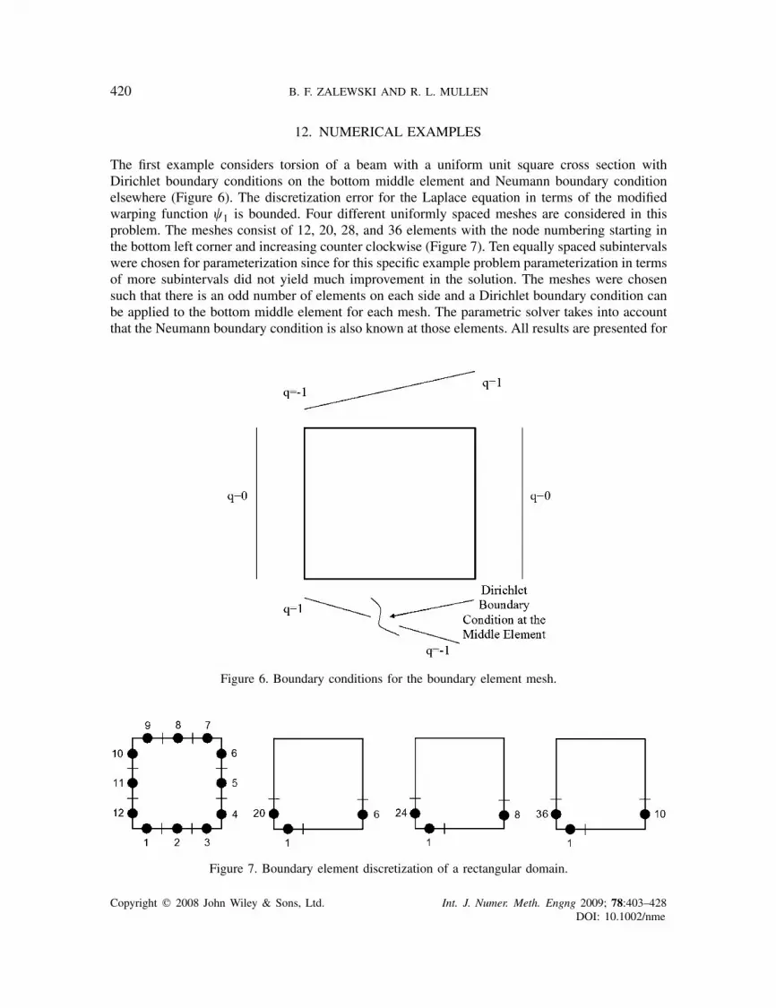
The first example considers torsion of a beam with a uniform unit square cross section withDirichlet boundary conditions on the bottom middle element and Neumann boundary conditionelsewhere (Figure 6). The discretization error for the Laplace equation in terms of the modifiedwarping function �1 is bounded. Four different uniformly spaced meshes are considered in thisproblem. The meshes consist of 12, 20, 28, and 36 elements with the node numbering starting inthe bottom left corner and increasing counter clockwise (Figure 7). Ten equally spaced subintervalswere chosen for parameterization since for this specific example problem parameterization in termsof more subintervals did not yield much improvement in the solution. The meshes were chosensuch that there is an odd number of elements on each side and a Dirichlet boundary condition canbe applied to the bottom middle element for each mesh. The parametric solver takes into accountthat the Neumann boundary condition is also known at those elements. All results are presented for

Figure 6. Boundary conditions for the boundary element mesh.

Figure 7. Boundary element discretization of a rectangular domain.



Table I. Solutions to the torsion problem for the 12 element mesh.

Exact ExactNode Lower lower upper Upper Interval Effectivityvalue bound bound bound bound width index

u1 0.0015 0.1099 14 0.3159 0.3143 2.2437

q2 − 13 − 1

313 0.3333 − 2

3 1.0000

u3 −0.3159 − 14 −0.1099 −0.0015 0.3143 2.2437

u4 −0.2515 − 14 −0.0567 0.0339 0.2853 1.4761

u5 −0.1265 −0.0567 0.0567 0.1529 0.2794 2.4640

u6 −0.0595 0.0567 14 0.3359 0.3954 2.0456

u7 0.0014 0.1099 14 0.3318 0.3304 2.3581

u8 −0.2107 −0.1099 0.1099 0.2107 0.4215 1.9174u9 −0.3315 − 1

4 −0.1099 −0.0014 0.3301 2.3560

u10 −0.3359 − 14 −0.0567 0.0595 0.3954 2.0456

u11 −0.1529 −0.0567 0.0567 0.1265 0.2794 2.4640

u12 −0.0339 0.0567 14 0.2515 0.2853 1.4761

Table II. Solution widths and effectivity indices for the torsion problem for different meshes.

Number of elements Node value Solution width Effectivity index

12 u4 0.2853 1.476120 u6 0.1990 1.457728 u8 0.1829 1.724236 u10 0.1648 1.8961

the 12 element mesh (Table I) and the widths of the solution as well as the effectivity indices arecompared for the right-hand side bottom corner elements 4, 6, 8, and 10 (Figure 7) for the differentmeshes (Table II). Figures 8–10 show the behavior of the solution bounds for the right bottomcorner elements 4, 6, 8, and 10 (Figure 7) for the respective meshes, whereas Figure 11 shows thesolution bounds of the right edge for the 12 element mesh. Figures 12 and 13 illustrate the solutionconvergence and computational expense with increasing number of subintervals, respectively, forthe 12 element mesh.

The second example demonstrates the behavior of the solution bounds for the L-shaped domain(Figure 14). The Dirichlet boundary conditions that are applied at all edges satisfy the Laplaceequation as:

∇2u = 0 in �

u = sinh(x)sin(y)

Four different uniformly spaced meshes consisting of 6, 12, 18, and 24 elements with the nodenumbering starting in the bottom left corner and increasing counter clockwise (Figure 14) are



Figure 8. Behavior of the interval solution width of the right bottom nodes with increasingmesh size for the torsion problem.

Figure 9. Behavior of the effectivity index of the right bottom nodes with increasingmesh size for the torsion problem.

considered. Ten equally spaced subintervals were chosen for parameterization since parameter-ization in terms of more subintervals did not yield much improvement in the solution for thisspecific example problem. The widths of the solution and the effectivity indices are compared forthe different meshes (Table III) at the left bottom elements 6, 12, 18, and 24 (Figure 14) for therespective meshes. Figures 15–17 show the behavior of the solution bounds for these elementswith decreasing element size. Figure 18 illustrates the behavior of the solution bounds for the leftedge for the different meshes considered.

13. CONCLUSION

The proposed method is capable of obtaining nearly sharp bounds for the discretization error inBEM. IBEM is formulated to account for the point-wise discretization error in the solutions in



Figure 10. Solution bounds of the right bottom nodes with different mesh sizes for the torsion problem.

Figure 11. Solution bounds on the right edge with different meshes for the torsion problem.



Figure 12. Solution bounds for element 4 in the 12 element mesh for the torsion problemwith increasing parameterization.

Figure 13. Computational cost of parameterization for element 4 in the 12element mesh torsion problem.

Figure 14. Boundary element discretization of the L-shaped domain.



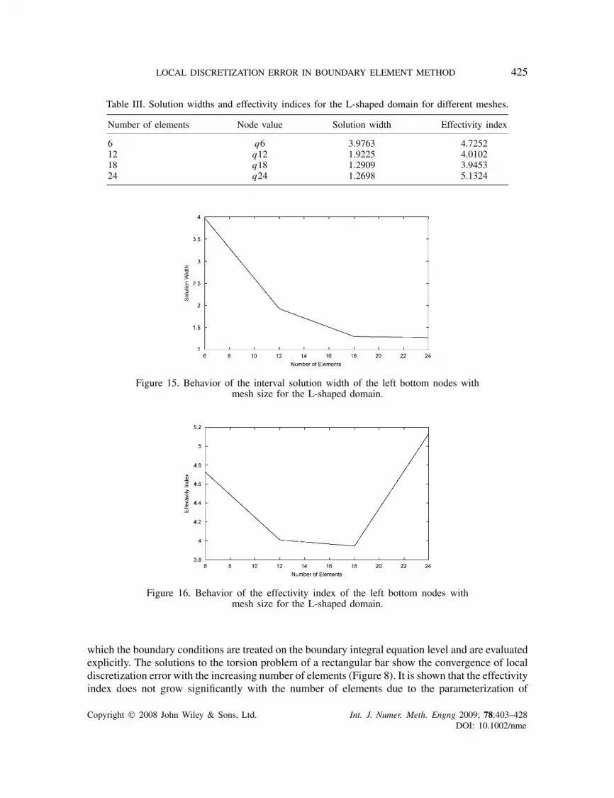
Table III. Solution widths and effectivity indices for the L-shaped domain for different meshes.

Number of elements Node value Solution width Effectivity index

6 q6 3.9763 4.725212 q12 1.9225 4.010218 q18 1.2909 3.945324 q24 1.2698 5.1324

Figure 15. Behavior of the interval solution width of the left bottom nodes withmesh size for the L-shaped domain.

Figure 16. Behavior of the effectivity index of the left bottom nodes withmesh size for the L-shaped domain.

which the boundary conditions are treated on the boundary integral equation level and are evaluatedexplicitly. The solutions to the torsion problem of a rectangular bar show the convergence of localdiscretization error with the increasing number of elements (Figure 8). It is shown that the effectivityindex does not grow significantly with the number of elements due to the parameterization of



Figure 17. Solution bounds for the left bottom nodes with different mesh sizes for the L-shaped domain.

Figure 18. Solution bounds for the left edge for the L-shaped domain for the different meshes.



interval matrices (Figure 9) and the solution bounds follow a general trend of the exact solutionbounds (Figures 10, 11). Overestimation in the results occurs due to the bounding of the kernelin the second integral on �2, parameterization not accounting fully for the unique location of thesource point on an element, although this dependency has been increased, and due to a solver ofthe interval linear system of equations which overestimates the solution. Further parameterizationdid not yield improvement in the solution, however, with increasing number of elements, finersubintervals may yield sharper results and therefore better control of the overestimation. The effectand the cost of the parameterization are studied for the 12 element mesh and it is shown that theoverestimation converges with the increasing number of subintervals parameterizing the system(Figure 12) [29]. The computational cost of parameterization (Figure 13), which is normalized bythe computational time needed to perform a conventional boundary element analysis, varies linearlyshowing the computational efficiency of the method. The second example shows the convergenceof the local disretization error for the L-shaped domain. The solution bounds (Figures 17, 18)and the interval solution width (Figure 15) converge with the increasing number of elements. Theeffectivity index is shown not to increase significantly with problem size due to the parameterizationof the interval equations (Figure 16). Although constant elements are used throughout the paper, themethod can be extended to higher-order approximations considering more than one source pointto vary within an element. Additional requirement that multiple nodes on an element must havean independent and unique location can be addressed readily using a discussed parameterization.

ACKNOWLEDGEMENTS

The authors would like to thank the support of the Center for Reliable Engineering Computing (REC).

REFERENCES

1. Zadeh LA. Fuzzy sets as a basis for theory of possibility. Fuzzy Sets and Systems 1978; 1:3–28.2. Dempster AP. Upper and lower possibilities induced by a multi-valued mapping. Annals of Mathematical Statistics

1967; 38:325–339.3. Shafer G. A Mathematical Theory of Evidence. Princeton University Press: Princeton, 1976.4. Mullen RL, Muhanna RL. Bounds of structural response for all possible loadings. Journal of Structural Engineering

(ASCE) 1999; 125(1):98–106.5. Muhanna RL, Mullen RL. Uncertainty in mechanics problems-interval-based approach. Journal of Engineering

Mechanics (ASCE) 2001; 127(6):557–566.6. Muhanna RL, Mullen RL, Zhang H. Penalty-based solution for the interval finite-element methods. Journal of

Engineering Mechanics (ASCE) 2005; 131(10):1102–1111.7. Moore RE. Interval Analysis. Prentice-Hall: Englewood Cliffs, NJ, 1966.8. Neumaier A. Interval Methods for Systems of Equations. Cambridge University Press: New York, NY, 1990.9. Alefeld G, Herzberger J. Introduction to Interval Computations. Academic Press: New York, NY, 1983.10. Gay DM. Solving interval linear equations. SIAM Journal on Numerical Analysis 1982; 19(4):858–870.11. Hansen E. Interval arithmetic in matrix computation. Journal of the Society for Industrial and Applied Mathematics,

Series B, Numerical Analysis 1965; 1(2):308–320.12. Jansson C. Interval linear system with symmetric matrices, skew-symmetric matrices, and dependencies in the

right hand side. Computing 1990; 46:265–274.13. Neumaier A. Overestimation in linear interval equations. SIAM Journal on Numerical Analysis 1987; 24(1):

207–214.14. Neumaier A. Rigorous sensitivity analysis for parameter-dependent systems of equations. Journal of Mathematical

Analysis and Applications 1989; 144:16–25.15. Rump SM. Rigorous sensitivity analysis for systems of linear and nonlinear equations.Mathematics of Computation

1990; 54(190):721–736.



16. Rump SM. Self-validating methods. Linear Algebra and its Applications 2001; 324:3–13.17. Sunaga T. Theory of interval algebra and its application to numerical analysis. RAAG Memoirs 3 1958; 3:29–46.18. Babuska I, Stroubolis T. The Finite Element Method and its Reliability. Clarendon Press: Oxford, 2001.19. Babuska I, Zienkiewicz OC, Cago J, Oliveira ER deA. Accuracy Estimates and Adaptive Refinements in Finite

Element Computaions. John Wiley and Sons: India, 1986.20. Zalewski BF, Mullen RL, Muhanna RL. Interval boundary element method in the presence of uncertain boundary

conditions, integration error, and truncation error. Engineering Analysis with Boundary Elements 2007; DOI:10.1016j.enganabound.2008.08.006.

21. Jaswon MA, Symm GT. Integral Equation Methods in Potential Theory and Elastostatics. Academic Press:London, 1977.

22. Carstensen C, Stephan EP. A posteriori error estimates for boundary element methods.Mathematics of Computation1995; 64(210):483–500.

23. Rencis JJ, Jong K-Y. An error estimator for boundary element computations. Journal of Engineering Mechanics(ASCE) 1989; 115:1993–2010.

24. Brebbia CA, Dominguez J. Boundary Elements: An Introductory Course, Computational Mechanics. McGraw-Hill:New York, NY, 1992.

25. Hartmann F. Introduction to Boundary Elements: Theory and Applications. Springer: New York, NY, 1989.26. Saada AS. Elasticity: Theory and Applications. Krieger Publishing Co.: Malabar, FL, 1993.27. Krawczyk R. Newton-algorithmen zur bestimmung von nullstellen mit fehlerschranken. Computing 1969; 4:

187–201.28. Dobner H. Kernel-splitting technique for enclosing the solution of Fredholm equations of the first kind. Reliable

Computing 2002; 8:179–469.29. Popova ED. Parametric interval linear solver. Numerical Algorithms 2004; 37:345–356.


local discretization error bounds using interval boundary element method

Documents