Absolute Bounds on the Mean of Sum, Product,etc.: A Probabilistic Extension of IntervalArithmeticScott Ferson1, Lev Ginzburg1,Vladik Kreinovich2, and Jorge Lopez21Applied Biomathematics, 100 North Country Road,Setauket, NY 11733, USA, fscott,levg@ramas.com2Computer Science Department, University of Texas at El PasoEl Paso, TX 79968, USA, vladik@cs.utep.eduAbstractWe extend the main formulas of interval arithmetic x1�x2 for di�erentarithmetic operations x1 � x2 to the case when, for each input xi, inaddition to the interval xi = [xi; xi] of possible values, we also know itsmean Ei (or an interval Ei of possible values of the mean), and we wantto �nd the corresponding bounds for x1 � x2 and its mean.1 Error Estimation for Indirect Measurements:An Important Practical ProblemA practically important class of statistical problems is related to data processing(indirect measurements). Some physical quantities y { such as the distance to astar or the amount of oil in a given well { are impossible or di�cult to measuredirectly. To estimate these quantities, we use indirect measurements, i.e., wemeasure some easier-to-measure quantities x1; : : : ; xn which are related to y bya known relation y = f(x1; : : : ; xn), and then use the measurement results exi(1 � i � n) to compute an estimate ey for y as ey = f(ex1; : : : ; exn):1

-: : :--exnex2ex1 -ey = f(ex1; : : : ; exn)f

For example, to �nd the resistance R, we measure current I and voltage V ,and then use the known relation R = V=I to estimate resistance as eR = eV =eI .Measurement are never 100% accurate, so in reality, the actual value xi ofi-th measured quantity can di�er from the measurement result exi. In proba-bilistic terms, xi is a random variable; its probability distribution describes theprobabilities of di�erent possible value of measurement error �xi def= exi � xi. Itis desirable to describe the error �y def= ey � y of the result of data processing:-: : :--�xn�x2�x1 -�yf

Often, we know (or assume) that the measurement error �xi of each directmeasurement is normally distributed with a known standard deviation �i, andthat measurement errors corresponding to di�erent measurements are indepen-dent. These assumptions { justi�ed by the central limit theorem, according towhich sums of independent identically distributed random variables with �nitemoments tend quickly toward the Gaussian distribution { underly the tradi-tional engineering approach to estimating measurement errors.In some situations, the error distributions are not Gaussian, but we knowtheir exact shape (e.g., lognormal). In many practical measurement situations,however, we only have partial information about the probability distributions[11, 12].2 The Need for Robust StatisticsTraditional statistical techniques deal (see, e.g., [15]) with the situations whenwe know the exact shape of the probability distributions. To deal with practical2

situations in which we only have a partial information about the distributions,special techniques have to be invented. Such techniques are called methodsof robust statistics. They are called robust because they are usually designedto provide guaranteed estimates, i.e., estimates which are valid for all possibledistributions from a given class [8, 15].3 Interval Computations as a Particular Case ofRobust StatisticsAn important case of partial information about a random variable x is when weknow (with probability 1) that x is within a given interval x = [x; x], but we haveno information about the probability distribution within this interval. In otherwords, x may be uniformly distributed on this interval, it may be deterministic(i.e., distributed in a single value with probability 1), distributed according toa truncated Gaussian, bimodal distribution { we do not know.So, we arrive at the following problem: for each of n random variablesx1; : : : ; xn, we know that it is located (with probability 1) within a given intervalxi = [xi; xi]. We do not know the distributions within the intervals, and we donot know whether the random variables xi are independent or not. What canwe then conclude about the probability distribution of y = f(x1; : : : ; xn)?Since the only information we have about each variable xi consists of itslower bound xi and upper bound xi, it is natural to ask for similar boundsy = [y; y] for y. As a result, we arrive at the following problem:GIVEN: an algorithm computing a function f(x1; : : : ; xn) from Rn to R andn intervals x1; : : : ;xn,TAKE: all possible joint probability distributions on Rn for which, for eachi, xi 2 xi with probability 1;FIND: the setY of all possible values of a random variable y = f(x1; : : : ; xn)for all such distributions.One can easily prove that Y is equal to the range f(x1; : : : ;xn) of the givenfunction f on given intervals, i.e., to ff(x1; : : : ; xn) jx1 2 x1; : : : ; xn 2 xng:-: : :--xnx2x1 -y = f(x1; : : : ;xn)f

3

Indeed:� If xi 2 xi with probability 1, then y belongs to the range with probabil-ity 1.� Vice versa, any point y from the range can be represented as f(x1; : : : ; xn)for some xi 2 xi, so to show that y 2 Y, we can take degenerate distribu-tions located at xi with probability 1.Q.E.D.The problem of computing the range of a given function f(x1; : : : ; xn) ongiven intervals xi is exactly the problem solved by interval computations. Themain interval computations approach to solving this problem is to take intoconsideration that inside the computer, every algorithm consists of elementaryoperations (arithmetic operations, min, max, etc.). For each elementary opera-tion f(x; y), if we know the intervals x and y for x and y, we can compute theexact range f(x;y): [x1; x1] + [x2; x1] = [x1 + x2; x1 + x2];[x1; x1]� [x2; x1] = [x1 � x2; x1 � x2];etc.; the corresponding formulas form the so-called interval arithmetic; see, e.g.,[9, 10]. We can therefore repeat the computations forming the program f step-by-step, replacing each operation with real numbers by the corresponding op-eration of interval arithmetic. It is known that, as a result, we get an enclosurefor the desired range.4 Comment About CorrelationIn the above proof, we considered the case when we have no information aboutthe correlation between the random variables. One can easily see that the sameproof shows that if we assume independence, we still get the same range.For functions of two variables, we can consider two additional cases:� when x1 and x2 are highly positively correlated, i.e., when there exists arandom variable t such that both x1 and x2 are non-decreasing functionsof t (crudely speaking, x1 is (non-strictly) increasing in x2), and� when xi is highly negatively correlated, i.e., when there exists a randomvariable t such that both x1 and x2 are non-decreasing functions of t(crudely speaking, when x1 is decreasing in x2).The above simple proof shows that in both cases, we get the same range Y asin the above case of no information about the correlation.4

5 New ProblemIn some practical situations, in addition to the lower and upper bounds on eachrandom variable xi, we know the bounds Ei = [Ei; Ei] on its mean Ei. In suchsituations, we arrive at the following problem:GIVEN: an algorithm computing a function f(x1; : : : ; xn) from Rn to R; nintervals x1; : : : ;xn, and n intervals E1; : : : ;En,TAKE: all possible joint probability distributions on Rn for which, for eachi, xi 2 xi with probability 1 and the mean Ei belongs to Ei;FIND: the setY of all possible values of a random variable y = f(x1; : : : ; xn)and the set E of all possible values of E def= E[y] for all such distri-butions:-: : :--xn;Enx2;E2x1;E1 -y;Ef

A similar problem can be formulated for the case when xi are known tobe independent, and for the cases when n = 2 and the values xi are highlypositively or highly negatively correlated.One can easily show that the interval part [y; y] of the result is the same asfor interval arithmetic, so what we really need to compute is the range E for E.Similarly to interval computations, our main idea is to �nd the correspondingformulas for the cases when n = 2 and f = � is one of the basic arithmeticoperations (+, �, �, 1=x, min, max): if we know two tuples (xi; Ei; Ei; xi),(i = 1; 2), what tuple describes possible values of y = x1 � x2?--x2;E2x1;E1 -y;E�5

In other words, to �nd these formulas, we want to solve the following prob-lem:GIVEN: values x1, x1, x2, x2, E1, E1, E2, E2, and an operation �,FIND: the valuesE def= minfE(x1 � x2) j all distributions of (x1; x2) for whichx1 2 [x1; x1]; x2 2 [x2; x2]; E[x1] 2 [E1; E1]; E[x2] 2 [E2; E2]gandE def= maxfE(x1 � x2) j all distributions of (x1; x2) for whichx1 2 [x1; x1]; x2 2 [x2; x2]; E[x1] 2 [E1; E1]; E[x2] 2 [E2; E2]g(plus restrictions on the correlation).In this paper, we provide the formulas for E and E.6 Main Results for the Case When We Knowthe Exact Values of E1 and E2In this section, we describe the formulas for the interval E of possible values ofE = E[y] for the case when the intervalsE1 and E2 are degenerate: Ei = [Ei; Ei]{ i.e., when we know the exact values of E1 and E2. In the following section,we show how to extend these formulas to the general case of non-degenerateintervals Ei.For addition, the answer is simple. Since E[x1 + x2] = E[x1] + E[x2], if y =x1 + x2, there is only one possible value for E = E[y]: the value E = E1 + E2.This value does not depend on whether we have correlation or nor, and whetherwe have any information about the correlation.Similarly, the answer is simple for subtraction: if y = x1 � x2, there is only onepossible value for E = E[y]: the value E = E1 �E2.For multiplication, if the variables x1 and x2 are independent, then E[x1 � x2] =E[x1] �E[x2]. Hence, if y = x1 � x2 and x1 and x2 are independent, there is onlyone possible value for E = E[y]: the value E = E1 �E2.The �rst non-trivial case is the case of multiplication in the presence of possiblecorrelation:6

Theorem 1. For multiplication y = x1 �x2, when we have no information aboutthe correlation,E = max(p1+p2�1; 0) �x1 �x2+min(p1; 1�p2) �x1 �x2+min(1�p1; p2) �x1 �x2+max(1� p1 � p2; 0) � x1 � x2;andE = min(p1; p2) � x1 � x2 +max(p1 � p2; 0) � x1 � x2 +max(p2 � p1; 0) � x1 � x2+min(1� p1; 1� p2) � x1 � x2;where pi def= (Ei � xi)=(xi � xi):For readers' convenience, proofs are placed in the special Appendix.Comment. Formulas for multiplication may sound very technical, but in reality,they make intuitive sense:� The probability pi can be interpreted as follows: if we only allow valuesxi and xi, then there is only one probability distribution on xi for whichthe average is exactly Ei. In this probability distribution, the probabilityp[xi] of xi is equal to pi, and the probability p[xi] of xi is equal to 1� pi.� In general, when we have two events A and B with known probabilitiesp(A) and p(B), then the probability of A&B can take any value from theinterval [p(A&B); p(A&B)], where p(A&B) def= max(p(A) + p(B)� 1; 0)and p(A&B) def= min(p(A); p(B)) (see, e.g., [16]). Indeed:{ the largest possible intersection is the smallest of the two sets, and{ the smallest possible intersection is when they are as far apart aspossible:� if p(A) + p(B) � 1, they can be completely disjoint hencep(A&B) = 0,� else we spread them as much as possible, so that p(A _ B) = 1hence p(A&B) = p(A) + p(B)� p(A&B) = p(A) + p(B)� 1.From this viewpoint, since p1 = p[x1] and p2 = p[x2], we can interpretmin(p1; p2) as p[x1&x2]. Similarly, we can interpret all other terms in theabove formulas, so we can rewrite the formulas for E and E as follows:E = p[x1&x2] � x1 � x2 + p[x1&x2] � x1 � x2 + p[x1&x2] � x1 � x2+p[x1&x2] � x1 � x2;7

E = p[x1&x2] � x1 � x2 + p[x1&x2] � x1 � x2 + p[x1&x2] � x1 � x2+p[x1&x2] � x1 � x2:Theorem 2. For multiplication y = x1 �x2, when x1 and x2 are highly positivelycorrelated, we have: E = E1 � E2andE = min(p1; p2) � x1 � x2 +max(p1 � p2; 0) � x1 � x2 +max(p2 � p1; 0) � x1 � x2+min(1� p1; 1� p2) � x1 � x2:Theorem 3. For multiplication y = x1 �x2, when x1 and x2 are highly negativelycorrelated, we have:E = max(p1+p2�1; 0) �x1 �x2+min(p1; 1�p2) �x1 �x2+min(1�p1; p2) �x1 �x2+max(1� p1 � p2; 0) � x1 � x2;and E = E1 � E2:Comment. One can easily see that the only di�erence between these formulas(corresponding to high correlation) and the formulas from Theorem 1 (cor-responding to all possible values of correlation) is that one of the bounds isreplaced by the value E1 � E2. From the common sense viewpoint, it is verynatural that the value E1 � E2 corresponding to the absence of correlation sep-arates cases with positive correlation (for which E[x1 � x2] is higher) and caseswith negative correlation (for which E[x1 � x2] is lower).For the inverse y = 1=x1, the �nite range is possible only when 0 62 x1. Withoutlosing generality, we can consider the case when 0 < x1. In this case, methodspresented in [14] lead to the following bound:Theorem 4. For the inverse y = 1=x1, the range of possible values of E isE = � 1E1 ; p1x1 + 1� p1x1 � :(Here p1 denotes the same value as in Theorems 1{3).For x1 � x2 = min(x1; x2) and x1 � x2 = max(x1; x2), there is an easy case: ifall the points from one of the intervals are not larger than all the points fromanother interval: 8

� If x1 � x2, then x1 2 x1 and x2 2 x2 imply x1 � x2. In this case,min(x1; x2) = x1 and max(x1; x2) = x2, hence E[min(x1; x2)] = E[x1] =E1 and E[max(x1; x2)] = E[x2] = E2.� Similarly, if x2 � x1, then x1 2 x1 and x2 2 x2 imply x2 � x1. In thiscase, min(x1; x2) = x2 and max(x1; x2) = x1, hence E[min(x1; x2)] =E[x2] = E2 and E[max(x1; x2)] = E[x1] = E1.What happens in all the other possible cases, i.e., when the intervals x1 and x2have a non-degenerate intersection?For min and max in case of independence, the results are as follows:Theorem 5. For minimum y = min(x1; x2), when x1 and x2 are independent,we have E = min(E1; E2) andE = p1 � p2 �min(x1; x2) + p1 � (1� p2) �min(x1; x2) + (1� p1) � p2 �min(x1; x2)+(1� p1) � (1� p2) �min(x1; x2):One can check that when x1 � x2 (corr., when x2 � x1), these formulas returnthe correct value E1 (corr., E2). The same is true for all the following theoremsabout min and max.Theorem 6. For maximum y = max(x1; x2), when x1 and x2 are independent,we have E = max(E1; E2) andE = p1 � p2 �max(x1; x2)+ p1 � (1� p2) �max(x1; x2)+ (1� p1) � p2 �max(x1; x2)+(1� p1) � (1� p2) �max(x1; x2):Comment. Both formulas have a natural probabilistic interpretation similar tothe formulas from Theorem 1: indeed, e.g., p1 � p2 is the probability p[x1&x2]under the condition that x1 and x2 are independent random variables.For the case when we have no information about the correlation between x1 andx2, we have the following results:Theorem 7. For minimum y = min(x1; x2), when we have no informationabout the correlation between x1 and x2, we have E = min(E1; E2) andE = max(p1 + p2 � 1; 0) �min(x1; x2) + min(p1; 1� p2) �min(x1; x2)+min(1� p1; p2) �min(x1; x2) + max(1� p1 � p2; 0) �min(x1; x2):9

Theorem 8. For maximum y = max(x1; x2), when we have no informationabout the correlation between x1 and x2, we have E = max(E1; E2) andE = min(p1; p2) �max(x1; x2) + max(p1 � p2; 0) �max(x1; x2)+max(p2 � p1; 0) �max(x1; x2) + min(1� p1; 1� p2) �max(x1; x2):What if we have high correlation? Let us �rst describe two easier cases:Theorem 9. For minimum y = min(x1; x2), when x1 and x2 are highly nega-tively correlated, the bounds E and E are the same as in Theorem 7.Theorem 10. For maximum y = min(x1; x2), when x1 and x2 are highlypositively correlated, the bounds E and E are the same as in Theorem 8.The other two cases are somewhat more complex:Theorem 11. For minimum y = min(x1; x2), when x1 and x2 are highlypositively correlated, E = min(E1; E2), and E is the smallest of the followingvalues:� the value min(E1; E2) that corresponds to a 1-point distribution;� the values p1 �min(x1; E2) + (1� p1) �min(x1; E2) and p2 �min(E1; x2) +(1� p2) �min(E1; x2) that correspond to 2-point distributions;� the solutions to the problemsp(1) � x1 + p(2) � x(1)2 + p(3) � x(2)1 ! minunder the conditionsx1 < x(1)2 < x(2)1 < x2; x(2)1 � x1; x2 � x(1)2 ;p(1) + p(2) + p(3) = 1;p(1) � x1 + (p(2) + p(3)) � x(2)1 = E1;(p(1) + p(2)) � x(1)2 + p(3) � x2 = E2;and p(1) � x2 + p(2) � x(1)1 + p(3) � x(2)2 ! minunder the conditionsx2 < x(1)1 < x(2)2 < x1; x(2)2 � x2; x1 � x(1)1 ;p(1) + p(2) + p(3) = 1;(p(1) + p(2)) � x(1)2 + p(3) � x2 = E1;p(1) � x2 + (p(2) + p(3)) � x(2)2 = E2:10

Comment. The corresponding optimization problems are not di�cult to solve.Indeed, e.g., in the �rst problem:p(1) � x1 + p(2) � x(1)2 + p(3) � x(2)1 ! minunder the conditionsx1 < x(1)2 < x(2)1 < x2; x(2)1 � x1; x2 � x(1)2 ;p(1) + p(2) + p(3) = 1;p(1) � x1 + (p(2) + p(3)) � x(2)1 = E1;(p(1) + p(2)) � x(1)2 + p(3) � x2 = E2;once we �x p(2) and p(3), we can describe p(1)a s 1�p(2)�p(3), and then explicitlydescribe x(1)2 and x(2)1 from the equations containing these values:x(2)1 = E1 � p(1)� x1p(2) + p(3) ; �x(1)2 = E2 � p(3) � x21� p(3) :Substituting these expressions into the optimized function, we get an explicitexpression for it in terms of p(2) and p(3):(1� p(2) � p(3)) � x1 + p(2) � E2 � p(3) � x21� p(3) + p(3) � E1 � p(1)� x1p(2) + p(3) ! minThe minimum is attained either at the endpoints of the corresponding intervals,or at a stationary point, where both partial derivatives are 0. Di�erentiatingwith respect to p(2) and p(3), we get simple equations relating p(2) and p(3).Theorem 12. For maximum y = max(x1; x2), when x1 and x2 are highlypositively correlated, E = max(E1; E2), and E is the largest of the followingvalues:� the value max(E1; E2) that corresponds to a 1-point distribution;� the values p1 �max(x1; E2) + (1� p1) �max(x1; E2) and p2 �max(E1; x2) +(1� p2) �max(E1; x2) that correspond to 2-point distributions;� the solutions to the problemsp(1) � x1 + p(2) � x(1)2 + p(3) � x(2)1 ! maxunder the conditions11

x1 > x(1)2 > x(2)1 > x2; x(2)1 � x1; x2 � x(1)2 ;p(1) + p(2) + p(3) = 1;p(1) � x1 + (p(2) + p(3)) � x(2)1 = E1;(p(1) + p(2)) � x(1)2 + p(3) � x2 = E2;and p(1) � x2 + p(2) � x(1)1 + p(3) � x(2)2 ! maxunder the conditionsx2 > x(1)1 > x(2)2 > x1; x(2)2 � x2; x1 � x(1)1 ;p(1) + p(2) + p(3) = 1;(p(1) + p(2)) � x(1)2 + p(3) � x1 = E1;p(1) � x2 + (p(2) + p(3)) � x(2)2 = E2:7 General Case: When Intervals Ei Are Non-DegenerateIn the previous section, we showed the bounds E and E for the moment E =E[x1 � x2] for the case when we know the moments Ei = E[xi]. We describedthese bounds for each of four correlation situations:i : when the variables x1 and x2 are independent;u : when the correlation between x1 and x2 is uknown;p : when we know that x1 and x2 are highly positively correlated;n : when we know that x1 and x2 are highly negatively correlated.Namely, for each arithmetic operation � and for each correlation situation c,we described these bounds as explicit functions of E1 and E2:E = f c�(E1; E2); E = fc�(E1; E2):If we only know the intervals E1 = [E1; E1] and E2 = [E2; E2] of possiblevalues of E1 and E2, then the set of possible values for E is a union of the setsof possible bounds for all E1 2 E1 and for all E2 2 E2. Thus, the resultingbounds E and E can be described by the following formulas:E = infE12E1;E22E2 f c�(E1; E2); E = supE12E1;E22E2 fc�(E1; E2):12

Let us show that for the elementary arithmetic operations, these formulas canbe simpli�ed into explicit analytical expressions.For addition � = +, f+(E1; E2) = f+(E1; E2) = E1+E2, therefore, the result-ing bounds E and E can be obtained by simply applying interval arithmetic:E = E1 +E2 and E = E1 +E2.For subtraction � = �, f�(E1; E2) = f�(E1; E2) = E1�E2, so we can also useinterval arithmetic: E = E1 �E2 and E = E1 �E2.For multiplication � = �, for the case of independent variables (c = i),f i�(E1; E2) = f i�(E1; E2) = E1 �E2;so we can use interval arithmetic as well: E = E1 �E2, i.e.,E = min(E1 � E2; E1 �E2; E1 � E2; E1 �E2);E = max(E1 �E2; E1 � E2; E1 � E2; E1 �E2):For multiplication under no information about dependence (c = u), the formulasfor fu�(E1; E2) and fu�(E1; E2) are given (by Theorem 1) in terms of the relatedprobabilities pi = (Ei�x1)=(xi�xi), so it is reasonable to replace the intervalsEi by the corresponding intervals for probabilities:pi = Ei � xiEi � xi ;i.e., pi = [pi; pi], where: pi = Ei � xiEi � xi ; pi = Ei � xiEi � xi :In terms of probability intervals, we get the following results:Proposition 1. For multiplication under no information about dependence, to�nd E, it is su�cient to consider the following combinations of p1 and p2:� p1 = p1 and p2 = p2; p1 = p1 and p2 = p2; p1 = p1 and p2 = p2;p1 = p1 and p2 = p2;� p1 = max(p1; 1� p2) and p2 = 1� p1 (if 1 2 p1 + p2); and� p1 = min(p1; 1� p2) and p2 = 1� p1 (if 1 2 p1 + p2).The smallest value of fu�(p1; p2) for all these cases is the desired lower bound E.13

Proposition 2. For multiplication under no information about dependence, to�nd E, it is su�cient to consider the following combinations of p1 and p2:� p1 = p1 and p2 = p2; p1 = p1 and p2 = p2; p1 = p1 and p2 = p2;p1 = p1 and p2 = p2;� p1 = p2 = max(p1; p2) (if p1 \ p2 6= ;); and� p1 = p2 = min(p1; p2) (if p1 \ p2 6= ;).The largest value of fu�(p1; p2) for all these cases is the desired upper bound E.Comment. The fact that we need to consider several cases, and then take themaximum for �nd E and the minimum to �nd E, is not surprising: a similarprocedure is used in interval arithmetic to compute the range for the productof two intervals.For multiplication in the case of high positive correlation, we havefp�(E1; E2) = E1 �E2;hence the smallest possible value E of E when E1 2 E1 and E2 2 E2 can becomputed as E = min(E1 � E2; E1 �E2; E1 � E2; E1 �E2):The upper bound fp�(E1; E2) is the same as for the case c = u, so to computeE, we can use the algorithm presented in Proposition 2.For multiplication in the case of high negative correlation, we havefp�(E1; E2) = E1 �E2;hence the largest possible value E of E when E1 2 E1 and E2 2 E2 can becomputed as E = max(E1 �E2; E1 � E2; E1 � E2; E1 �E2):The lower bound fp�(E1; E2) is the same as for the case c = u, so to computeE, we can use the algorithm presented in Proposition 1.Proposition 3. When 0 < x1, for the inverse y = 1=x1, the range of possiblevalues of E is E = � 1E1 ; p1x1 + 1� p1x1 � :14

Proposition 4. For minimum y = min(x1; x2), when x1 and x2 are indepen-dent, we have:E = p1 � p2 �min(x1; x2) + p1 � (1� p2) �min(x1; x2) + (1� p1) � p2 �min(x1; x2)+(1� p1) � (1� p2) �min(x1; x2);and E = min(E1; E2):Proposition 5. For maximum y = max(x1; x2), when x1 and x2 are indepen-dent, we have: E = max(E1; E2)andE = p1 � p2 �max(x1; x2)+ p1 � (1� p2) �max(x1; x2)+ (1� p1) � p2 �max(x1; x2)+(1� p1) � (1� p2) �max(x1; x2):Proposition 6. For minimum under no information about dependence, E =min(E1; E2); to �nd E, we must consider all combinations of p1 and p2 fromProposition 1 and take the smallest possible value of fumin(p1; p2) for all thesecombinations.Proposition 7. For maximum under no information about dependence, E =max(E1; E2); to �nd E, we must consider all combinations of p1 and p2 fromProposition 2 and take the largest possible value of fumax(p1; p2) for all thesecombinations.Proposition 8. For minimum y = min(x1; x2), when x1 and x2 are highlynegatively correlated, the bounds E and E are the same as in Proposition 6.Proposition 9. For maximum y = min(x1; x2), when x1 and x2 are highlypositively correlated, the bounds E and E are the same as in Proposition 7.For the other two cases, we only have explicit formulas for one of the bounds:Proposition 10. For minimum under highly positive correlation, E =min(E1; E2).Proposition 11. For maximum under highly negative correlation, E =max(E1; E2).15

8 From Elementary Arithmetic Operations toGeneral AlgorithmsSo far, we have discussed how to �nd the intervals of possible values for E[y]for the case when y = f(x1; : : : ; xn) is an elementary arithmetic operation.In practice, of course, we are interested largely in the situations when f is acomplex algorithm. How can we �nd the set of possible values of E for thismore complex case?One possibility, as we have mentioned, is to follow the example of straight-forward interval computations: represent the algorithm f as a \code list" (asequence of elementary arithmetic operation), and replace each operation bythe corresponding operation with the pairs hxi;Eii. Similarly to the case of in-terval computations, we can prove that the resulting interval eE is an enclosurefor the desired interval E.Sometimes we get the exact interval, but often we get a proper superset ofthe desired interval E. How can we �nd the actual range of E = E[y]? At�rst glance, the exact formulation of this problem requires that we use in�nitelymany variables, because we must describe all possible probability distributionson the box x1�: : :�xn (or, in the independent case, all possible tuples consistingof distributions on all n intervals x1; : : : ;xn). It turns out, however, that we canreformulate these problems in equivalent forms that require only �nitely manyvariables:Proposition 12. Let n be an integer, x1; : : : ;xn;E1 � x1; : : : ;En � xn beintervals, and let f(x1; : : : ; xn) be a continuous function of n real variables.Then, the range E = [E;E] of possible values of E[y], where y = f(x1; : : : ; xn),over all possible distributions on the box x1 � : : : � xn for which xi 2 xi andE[xi] 2 Ei, can be determined as follows:� E is a solution to the following constraint optimization problem:nXj=0 p(j) � f(x(j)1 ; : : : ; x(j)n )! minunder the conditions nXj=0 p(j) = 1;p(j) � 0; for all j;xi � x(j)i � xi for all i; j;Ei � nXj=0 p(j) � x(j)i � Ei for all i:16

� E is a solution to the constraint optimization problem:nXj=0 p(j) � f(x(j)1 ; : : : ; x(j)n )! maxunder the same constraints.Proposition 13. Let n be an integer, x1; : : : ;xn;E1 � x1; : : : ;En � xn beintervals, and let f(x1; : : : ; xn) be a continuous function of n real variables.Then, the range E = [E;E] of possible values of E[y], where y = f(x1; : : : ; xn),over all possible independent distributions x1; : : : ;xn for which xi 2 xi andE[xi] 2 Ei, can be determined as follows:� E is a solution to the following constraint optimization problem:X"12f�;+g : : : X"n2f�;+g p"11 � : : : � p"nn � f(x"11 ; : : : ; x"nn )! minunder the conditions p�i + p+i = 1 for all i;p�i � 0 and p+i � 0; for all i;xi � x�i � x+i � xi for all i;Ei � p� � x�i + p+i � x+i � Ei for all i:� E is a solution to the constraint optimization problem:X"12f�;+g : : : X"n2f�;+g p"11 � : : : � p"nn � f(x"11 ; : : : ; x"nn )! maxunder the same constraints.For convex and concave functions, these results can be further simpli�ed:Proposition 14. Let n be an integer, x1; : : : ;xn;E1 � x1; : : : ;En � xn beintervals, and let f(x1; : : : ; xn) be a convex function of n real variables. Then,the range E = [E;E] of possible values of E[y], where y = f(x1; : : : ; xn), over allpossible distributions on the box x1� : : :�xn for which xi 2 xi and E[xi] 2 Ei,is as follows: E = f(E1; : : : ; En);and E is a solution to the following constraint optimization problem:nXj=0 p(j) � f(x(j)1 ; : : : ; x(j)n )! max17

under the conditions nXj=0 p(j) = 1;p(j) � 0; for all j;x(j)i = xi or x(j)i = xi for all i; j;Ei � nXj=0 p(j) � x(j)i � Ei for all i:Proposition 15. Let n be an integer, x1; : : : ;xn;E1 � x1; : : : ;En � xn beintervals, and let f(x1; : : : ; xn) be a concave function of n real variables. Then,the range E = [E;E] of possible values of E[y], where y = f(x1; : : : ; xn), over allpossible distributions on the box x1� : : :�xn for which xi 2 xi and E[xi] 2 Ei,is as follows: E = f(E1; : : : ; En);and E is a solution to the following constraint optimization problem:nXj=0 p(j) � f(x(j)1 ; : : : ; x(j)n )! minunder the conditions nXj=0 p(j) = 1;p(j) � 0; for all j;x(j)i = xi or x(j)i = xi for all i; j;Ei � nXj=0 p(j) � x(j)i � Ei for all i:Proposition 16. Let n be an integer, x1; : : : ;xn;E1 � x1; : : : ;En � xn beintervals, and let f(x1; : : : ; xn) be a convex function of n real variables. Then,the range E = [E;E] of possible values of E[y], where y = f(x1; : : : ; xn), over allpossible independent distributions x1; : : : ;xn for which xi 2 xi and E[xi] 2 Ei,is as follows: E = f(E1; : : : ; En);E = X"12f�;+g : : : X"n2f�;+g p"11 � : : : � p"nn � f(x"11 ; : : : ; x"nn );where p+i def= pi, p�i def= 1� pi, x�i def= xi and x+i def= xi.18

Proposition 17. Let n be an integer, x1; : : : ;xn;E1 � x1; : : : ;En � xn beintervals, and let f(x1; : : : ; xn) be a concave function of n real variables. Then,the range E = [E;E] of possible values of E[y], where y = f(x1; : : : ; xn), over allpossible independent distributions x1; : : : ;xn for which xi 2 xi and E[xi] 2 Ei,is as follows:E = X"12f�;+g : : : X"n2f�;+g p"11 � : : : � p"nn � f(x"11 ; : : : ; x"nn );E = f(E1; : : : ; En);where p+i def= pi, p�i def= 1� pi, x�i def= xi and x+i def= xi.Similar results can be proven for the case when n = 2 and x1 and x2 are highlycorrelated:Proposition 18. Let x1;x2;E1 � x1;E2 � x2 be intervals, and let f(x1; x2)be a continuous function of two real variables. Then, the range E = [E;E] ofpossible values of E[y], where y = f(x1; x2), over all possible distributions highlypositively correlated distributions on the box x1� : : :�xn for which xi 2 xi andE[xi] 2 Ei, can be determined as follows:� E is a solution to the following constraint optimization problem:2Xj=0 p(j) � f(x(j)1 ; x(j)n )! minunder the conditions 2Xj=0 p(j) = 1;p(j) � 0; for all j;xi � x(j)i � xi for all i; j;Ei � nXj=0 p(j) � x(j)i � Ei for all i;x(j)i � x(j+1)i for all i; j:� E is a solution to the constraint optimization problem:2Xj=0 p(j) � f(x(j)1 ; x(j)2 )! maxunder the same constraints. 19

Proposition 19. Let x1;x2;E1 � x1;E2 � x2 be intervals, and let f(x1; x2)be a continuous function of two real variables. Then, the range E = [E;E] ofpossible values of E[y], where y = f(x1; x2), over all possible distributions highlynegatively correlated distributions on the box x1� : : :�xn for which xi 2 xi andE[xi] 2 Ei, can be determined as follows:� E is a solution to the following constraint optimization problem:2Xj=0 p(j) � f(x(j)1 ; x(j)n )! minunder the conditions 2Xj=0 p(j) = 1;p(j) � 0; for all j;xi � x(j)i � xi for all i; j;Ei � nXj=0 p(j) � x(j)i � Ei for all i;x(j)1 � x(j+1)1 and x(j)2 � x(j+1)2 for all j:� E is a solution to the constraint optimization problem:2Xj=0 p(j) � f(x(j)1 ; x(j)2 )! maxunder the same constraints.9 From Intervals and First-Order Moments toHigher-Order MomentsSo far, we have provided explicit formulas for the elementary arithmetic opera-tions f(x1; : : : ; xn) for the case when we know the �rst order moments. Whatif, in addition to that, we have some information about second order (and/orhigher order) moments of xi? What will we be then able to conclude aboutthe moments of y? Partial answers to this question are given in [5, 14]; it isdesirable to �nd a general answer.Similarly to the case of �rst moments, we can reduce the correspondingproblems to the constraint optimization problems with �nitely many variables(the proof is similar). For example, when, in addition to intervals Ei that20

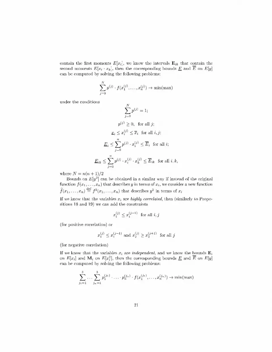
contain the �rst moments E[xi], we know the intervals Eik that contain thesecond moments E[xi � xk ], then the corresponding bounds E and E on E[y]can be computed by solving the following problems:NXj=0 p(j) � f(x(j)1 ; : : : ; x(j)n )! min(max)under the conditions NXj=0 p(j) = 1;p(j) � 0; for all j;xi � x(j)i � xi for all i; j;Ei � nXj=0 p(j) � x(j)i � Ei for all i;Eik � nXj=0 p(j) � x(j)i � x(j)k � Eik for all i; k;where N = n(n+ 1)=2.Bounds on E[y2] can be obtained in a similar way if instead of the originalfunction f(x1; : : : ; xn) that describes y in terms of xi, we consider a new functionef(x1; : : : ; xn) def= f2(x1; : : : ; xn) that describes y2 in terms of xi.If we know that the variables xi are highly correlated, then (similarly to Propo-sitions 18 and 19) we can add the constraintsx(j)i � x(j+1)i for all i; j(for positive correlation) orx(j)1 � x(j+1)1 and x(j)2 � x(j+1)2 for all j(for negative correlation).If we know that the variables xi are independent, and we know the bounds Eion E[xi] and Mi on E[x2i ], then the corresponding bounds E and E on E[y]can be computed by solving the following problems:3Xj1=1 : : : 3Xjn=1 p(j1)1 � : : : � p(jn)n � f(x(j1)1 ; : : : ; x(jn)n )! min(max)21

under the conditions 3Xj=1 p(j)i = 1 for all i;p(j)i � 0; for all i; j;xi � x(j)i � xi for all i; j;Ei � 3Xj=1 p(j)i � x(j)i � Ei for all i;M i � 3Xj=1 p(j)i � �x(j)i �2 �M i for all i:ConclusionsIn addition to intervals, we sometimes know the means Ei or intervals [Ei; Ei]that contain the corresponding means. In this paper, we have described how togeneralize interval arithmetic to this new case.AcknowledgmentsThis work was supported in part by NASA under cooperative agreement NCC5-209 and grant NCC2-1232, by NSF grants CDA-9522207, ERA-0112968 and9710940Mexico/Conacyt, by the Future Aerospace Science and Technology Pro-gram (FAST) Center for Structural Integrity of Aerospace Systems, e�ort spon-sored by the Air Force O�ce of Scienti�c Research (AFOSR), Air Force MaterielCommand, USAF, under grants numbers F49620-95-1-0518 and F49620-00-1-0365, by the IEEE/ACM SC2001 Minority Serving Institutions ParticipationGrant, and by Small Business Innovation Research grant 9R44CA81741 to Ap-plied Biomathematics from the National Cancer Institute (NCI), a componentof the National Institutes of Health (NIH). The opinions expressed herein arethose of the author(s) and not necessarily those of NASA, NSF, AFOSR, NCI,or the NIH. This work was partly done when one of the authors (V.K.) was aVisiting Faculty Member at the Fields Institute for Research in MathematicalSciences (Toronto, Canada).The authors are thankful to all the participants of the 2002 SIAM Workshopon Validated Computing and of the 2002 Informal Working Group on ValidatedMethods for Optimization, especially to Dan Berleant, George Corliss, R. BakerKearfott, Weldon Lodwick, and Bill Walster, for valuable discussions.22

References[1] D. Berleant, \Automatically veri�ed arithmetic with both intervals andprobability density functions", Interval Computations, 1993, No. 2, pp. 48{70.[2] D. Berleant, \Automatically veri�ed arithmetic on probability distributionsand intervals", In: R. B. Kearfott and V. Kreinovich (eds.) Applications ofInterval Computations, Kluwer, Dordrecht, 1996.[3] D. Berleant and C. Goodman-Strauss, \Bounding the results of arithmeticoperations on random variables of unknown dependency using intervals",Reliable Computing, 1998, Vol. 4, No. 2, pp. 147{165.[4] S. Ferson, W. Root and R. Kuhn, RAMAS Risk Calc: Risk Assessment withUncertain Numbers, Applied Biomathematics, Setauket, NY, 1999.[5] S. Ferson, D. Myers, and D. Berleant, Distribution-free risk analysis: I.Range, mean, and variance, Applied Biomath. Technical Report, 2001.[6] M. J. Frank, R. B. Nelson, and B. Schweizer, \Best-possible bounds for thedistribution of a sum { a problem of Kolmogorov", Probability Theory andRelated Fields, 1987, Vol. 74, pp. 199{211.[7] L. A. Goodman, \On the exact variance of products", Journal of AmericanStatistical Association, 1960, Vol. 55, pp. 718{713.[8] P. J. Huber, Robust statistics, Wiley, New York, 1981.[9] L. Jaulin, M. Kei�er, O. Didrit, and E. Walter, Applied Interval Analy-sis, with Examples in Parameter and State Estimation, Robust Control andRobotics, Springer-Verlag, Berlin, 2001.[10] R. E. Moore, Methods and Applications of Interval Analysis, SIAM,Philadelphia, 1979.[11] P. V. Novitskii and I. A. Zograph, Estimating the Measurement Errors,Leningrad: Energoatomizdat, 1991 (in Russian).[12] A. I. Orlov, \How often are the observations normal?", Industrial Labora-tory, 1991, Vol. 57, No. 7, pp. 770{772.[13] J. Pesonen and E. Hyv�onen, \Interval Approach Challenges Monte CarloSimulation", Reliable Computing, 1996, Vol. 2, No. 2, pp. 155{160.[14] N. C. Rowe, \Absolute bounds on the mean and standard deviation oftransformed data for constant-sign-derivative transformations", SIAM Jour-nal of Scienti�c Statistical Computing, 1988, Vol. 9, pp. 1098{1113.23

[15] H. M. Wadsworth, Jr. (eds.), Handbook of statistical methods for engineersand scientists, McGraw-Hill Publishing Co., New York, 1990.[16] P. Walley, Statistical reasoning with imprecise probabilities, Chapman andHall, N.Y., 1991.[17] G. W. Walster, \Philosophy and practicalities of interval arithmetic", In:R. E. Moore (ed.), Reliability in Computing, 1988, pp. 307{323.[18] R. Williamson and T. Downs, \Probabilistic arithmetic I: numerical meth-ods for calculating convolutions and dependency bounds", InternationalJournal of Approximate Reasoning, 1990, Vol. 4, pp. 89{158.Appendix: ProofsProof of Theorem 1. To get the desired bounds E and E, we must considerthe values E[x1 � x2] for all possible probability distributions on the box x1 �x2 for which E[x1] = E1 and E[x2] = x2. To describe a general probabilitydistribution, we must use in�nitely many parameters, and hence, this problemis di�cult to solve directly.To make the problem simpler, we will show that a general distribution withE[xi] = Ei can be simpli�ed without changing the values E[xi] and E[x1 � x2].Thus, to describe possible values of E[x1 � x2], we do not need to consider allpossible distributions, it is su�cient to consider only the simpli�ed ones.We will describe the simpli�cation for discrete distributions that concentrateon �nitely many points x(j) = (x(j)1 ; x(j)2 ), 1 � j � N . An arbitrary probabil-ity distribution can be approximated by such distributions, so we do not loseanything by this restriction.So, we have a probability distribution in which the point x(1) appears withthe probability p(1), the point x(2) appears with the probability p(2), etc. Let usmodify this distribution as follows: pick a point x(j) = (x(j)1 ; x(j)2 ) that occurswith probability p(j), and replace it with two points: x(j) = (x1; x(j)2 ) withprobability p(j) � p(j) and x(j) = (x1; x(j)2 ) with probability p(j) � p(j), wherep(j) def= x(j)1 � x1x1 � x1and p(j) def= 1� p(j) :24

@�x(j)�x(j) x(j)-Here, the values p(j) and p(j) = 1 � p(j) are chosen in such a way thatp(j) � x1 + p(j) � x1 = x(j)1 . Due to this choice,p(j) � p(j) � x1 + p(j) � p(j) � x1 = p(j) � x(j)1 ;hence for the new distribution, the mathematical expectation E[x1] is the sameas for the old one. Similarly, we can prove that the values E[x2] and E[x1 � x2]do not change.We started with a general discrete distribution with N points for each ofwhich x(j)1 could be inside the interval x1, and we have a new distribution forwhich � N � 1 points have the value x1 inside this interval. We can perform asimilar replacement for all N points and get a distribution with the same valuesof E[x1], E[x2], and E[x1 �x2] as the original one but for which, for every point,x1 is equal either to x1, or to x1.For the new distribution, we can perform a similar transformation relativeto x1 and end up { without changing the values x1 { with the distribution forwhich always either x2 = x1 or x2 = x2:

@�?6x(j)x(j)

x(j)Thus, instead of considering all possible distributions, it is su�cient to con-sider only distributions for which x1 2 fx1; x1g and x2 2 fx2; x2g. In otherwords, it is su�cient to consider only distributions which are located in the fourcorner points (x1; x2), (x1; x2), (x1; x2), and (x1; x2) of the box x1 � x2:25

@� @�@� @�Such distribution can be characterized by the probabilities of these fourpoints; we will denote these probabilities by p(x1&x2), p(x1&x2), p(x1&x2),and p(x1&x2). So, we have a �nite-parametric family of distributions.These four probabilities cannot be given arbitrarily, they must satisfy threeequations: their sum must be equal to 1:p(x1&x2) + p(x1&x2) + p(x1&x2) + p(x1&x2) = 1;and we must have the given values of E[x1] and E[x2].Since x1 takes only two possible values x1 and x1, the condition E[x1] = E1can be described as p(x1) � x1 + p(x1) � x1 = E1;where p(x1) def= p(x1&x2) + p(x1&x2)is the total probability of x1, and p(x1) = 1 � p(x1) is the total probability ofx1. From the condition that(1� p(x1)) � x1 + p(x1) � x1 = E1;we conclude that p(x1) = Ei � xixi � xi ;i.e., that the probability p(x1) coincides with the quantity p1 de�ned in Theorem1. Thus, we must have p(x1&x2) + p(x1&x2) = p1.Similarly, we can conclude that the probability p(x2) (that x2 = x2) coin-cides with the quantity p2 de�ned in Theorem 1, and thus, that p(x1&x2) +p(x1&x2) = p2.We have three conditions on four probabilities. Thus, we have, in e�ect,a 1-dimensional family of distributions, for which it is much easier to �nd thesmallest and the largest possible values of E[x1 � x2].Reduction to a 4-corner distribution is a general fact, true for both desiredbounds E and E. Now, depending on which bound we want to estimate, wewill perform di�erent transformations. Since we are interested not only in the26

general case, but also in the cases of \co-monotonicity" (highly positive andhighly negative correlation), it makes sense to ask a natural question: whendoes \co-monotonicity" increase E[x1 � x2]? when does it decrease it?To answer this question, we will also consider discrete distributions, thistime { distributions in which N points x(j) = (x(j)1 ; x(j)2 ) all have equal prob-abilities. It is also well known that every probability distribution on the boxcan be approximated by such distributions (in such a way that moments areapproximated as well). For such distributions:� highly positive correlation means that we can order the points x(j) in sucha way that when i < j, we have x(i)1 � x(j)1 and x(i)2 � x(j)2 ;� highly negative correlation means that we can order the points x(j) in sucha way that when i < j, we have x(i)1 � x(j)1 and x(i)2 � x(j)2 .Let us �rst consider the case of highly positive correlation. Reformulating theabove property, we can see that a distribution is not highly positively correlatedif and only if there exist points i and j for which x(i)1 < x(j)1 and x(i)2 > x(j)2 .We can \correct" this obstacle to highly positive correlation by \swapping" thesecond components of these points, i.e., by replacing x(i) and x(j) with two newpoints x(i)new = (x(i)1 ; x(j)2 ) and x(j)new = (x(j)1 ; x(i)2 ). It is easy to see that this swapdoes not change E[x1] = (1=N) � NXk=1x(k)1 and E[x2] = (1=N) � NXk=1 x(k)2 . Howdoes it a�ect E[x1 � x2] = (1=N) � NXk=1x(k)1 � x(k)2 ? The only two terms that arechanged are terms corresponding to k = i and k = j:� For the original points, the sum of these two terms is equal to x(i)1 � x(i)2 +x(j)1 � x(j)2 .� For the new points, the corresponding sum is equal to x(i)1 �x(j)2 +x(j)1 �x(i)2 .� Therefore, the di�erence between the new and the old values of E[x1 � x2]is equal to:1N � (x(i)1 � x(j)2 + x(j)1 � x(i)2 � (x(i)1 � x(i)2 + x(j)1 � x(j)2 )):One can easily see that this di�erence is equal to1N � (x(i)1 � x(j)1 ) � (x(j)2 � x(i)2 ):Thus, when we have a distribution which is not highly positively correlated, i.e.,for which x(i)1 < x(j)1 and x(i)2 > x(j)2 for some i and j, the above swap not only27

deletes this violation of highly positive correlation, it also increases the valueE[x1 � x2].So, if we are interested in the maximum of E[x1 � x2], we can perform theseswaps until no further swaps are possible (since there are only �nitely manyrearrangement of the original second components, and each swap increases thevalue of E[x1 � x2], this process has to stop). So, we arrive at the followingconclusion: when we are looking for the maximum of E[x1 � x2], we only needto consider highly positively correlated distributions.Similarly, a distribution is not highly negatively correlated if and only if thereexist points i and j for which x(i)1 < x(j)1 and x(i)2 < x(j)2 . In this case, a similarswap leaves E[x1] and E[x2] unchanged but decreases the value E[x1 �x2]. Thus,when we are looking for the minimum of E[x1 � x2], we only need to considerhighly negatively correlated distributions.We have already proven that it is su�cient to consider only distributionslocated at the four corners of the box x1 � x2. Now, we know something extra:� If we look for the maximum of E[x1 � x2], then it is su�cient to considerthe case of highly positive correlation. For a 4-corner distribution thismeans that we cannot have both points (x1; x2) and (x1; x2) { for one ofthese points, the probability should be equal to 0:@�@�@�

@�@�@�� If we look for the minimum of E[x1 � x2], then it is su�cient to considerthe case of highly negative correlation. For a 4-corner distribution thismeans that we cannot have both points (x1; x2) and (x1; x2) { for one ofthese points, the probability should be equal to 0:

28

@�@�

@�@�@�

@�Let us �rst consider the case of E.� If p(x1&x2) = 0, then p(x1&x2) = p1. So, from p(x1&x2)+p(x1&x2) =p2, we can conclude that p2 � p1, and p(x1&x2) = p2�p1. The remainingprobability p(x1&x2) can be determined from the condition that the sumof all three probabilities is 1, and is, therefore, equal to 1� p2.� If p(x1&x2) = 0, then p(x1&x2) = p2. So, from p(x1&x2)+p(x1&x2) =p1, we can conclude that p1 � p2, and p(x1&x2) = p1�p2. The remainingprobability p(x1&x2) can be determined from the condition that the sumof all three probabilities is 1, and is, therefore, equal to 1� p1.One can see that in both cases,p(x1&x2) = min(p1; p2); p(x1&x2) = max(p1 � p2; 0);p(x1&x2) = max(p2 � p1; 0); p(x1&x2) = min(1� p1; 1� p2):Therefore, the mathematical expectation E[x1 � x2] of x1 � x2 is equal exactly tothe expression from Theorem 1.For E, the situation is similar:� If p(x1&x2) = 0, then p(x1&x2) = p(x1) = 1 � p1 and p(x1&x2) =p(x1) = 1� p2. The remaining probability p(x1&x2) can be determinedfrom the condition that the sum of all three probabilities is 1, and is,therefore, equal to 1� (1�p1)� (1�p2) = p1+p2�1. Since probabilitiesare non-negative, this is only possible when p1 + p2 � 1.� If p(x1&x2) = 0, then p(x1&x2) = p1 and p(x1&x2) = p2. The remain-ing probability p(x1&x2) can be determined from the condition that thesum of all three probabilities is 1, and is, therefore, equal to 1� p1 � p2.Since probabilities are non-negative, this is only possible when p1+p2 � 1.One can see that in both cases, p(x1&x2) = max(p1 + p2 � 1; 0), p(x1&x2) =min(p1; 1�p2), p(x1&x2) = min(1�p1; p2), and p(x1&x2) = max(1�p1�p2; 0).Therefore, the mathematical expectation E[x1 � x2] of x1 � x2 is equal exactly tothe expression from Theorem 1. 29

The theorem is proven.Proof of Theorem 2. In the proof of Theorem 1, we have shown that themaximum of E[x1 �x2] is attained at a highly positively correlated distribution;therefore, the maximum E of E[x1 � x2] over all possible distributions shouldbe equal to the maximum of E[x1 � x2] over all highly positively correlateddistributions.To complete the proof of the theorem, it is therefore su�cient to prove thatthe lower bound E is equal to E1 � E2. The value E1 � E2 can be attained by adegenerate distribution concentrated on the point (E1; E2) with probability 1.So, to complete the proof of the theorem, we will show that by replacing theoriginal distribution by the degenerate distribution concentrated on its average(E1; E2), we decrease E[x1 � x2].Similar to Theorem 1, we can, without loss of generality, consider discretedistributions that concentrate on �nitely many points x(j) = (x(j)1 ; x(j)2 ), 1 �j � N . So, we have a probability distribution in which the point x(1) appearswith the probability p(1), the point x(2) appears with the probability p(2), etc.As we have mentioned in the proof of Theorem 1, the fact that the distributionis highly positively correlated means that we can order the points x(j) in sucha way that when i < j, we have x(i)1 � x(j)1 and x(i)2 � x(j)2 . Let us thereforeassume that the points are ordered this way.We will show that when we replace, in our distribution, the two neighboringpoints x(i) and x(i+1) by their average x = � � x(i+1) + (1 � �) � x(i) (where� = p(i+1)=(p(i) + p(i+1))) with probability p(i) + p(i+1), then:(1) we preserve E[x1] and E[x2];(2) we preserve the highly positive correlation property, and(3) the value E[x1 � x2] either decreases or stays the same.@� @���� ��x(i) x x(i+1)

Once this is proven, we will have a new highly positively correlated distribu-tion with N � 1 points and smaller (or same) value of E[x1 � x2]. We can applythe same reduction to the new distribution, etc., until we have only a single30

point x = (x1; x2) left. Since our transformation preserves the values E[x1] andE[x2], we have x1 = E1 and x2 = E2 and hence, E[x1 � x2] = E1 � E2. Sincethe value E[x1 �x2] cannot increase under our transformations, we can thereforeconclude that the original value of E[x1 � x2] was larger or equal to E1 � E2 {i.e., that E1 �E2 is indeed the lower bound.Let us proceed with proof of the three properties of the above transformation.(1) Let us �rst prove that the above transformation preserves E[x1] (for E[x2]the proof is the same). Indeed, after the transformation, the only change in theoriginal expression E[x1] = NXk=1 p(k) � x(k)1 is that we replace the sum p(i) � x(i)1 +p(i+1) � x(i+1)1 of i-th and (i + 1)-th terms by the new term (p(i) + p(i+1)) � x1,i.e., by de�nition of x, by the term(p(i) + p(i+1)) � (� � x(i+1)1 + (1� �) � x(i)1 ):By de�nition of �, this expression is exactly equal to the original sum (this iswhy we chose the above �). So, the values E[xi] are indeed unchanged.(2) It is also easy to show that the distribution continues to be strictly positivelycorrelated. To prove it, we must show two things:(2a) that if k < i, then x(k)1 � x1 and x(k)2 � x2; and(2b) that if i < k, then xi � x(k)1 and x2 � x(k)2 .Let us prove the �rst property (2a) (the second property (2b) is proven in thesame way). Since the original distribution was highly positively correlated, wehave x(k)1 � x(k)1 and x(k)1 � x(i+1)1 . Multiplying the �rst inequality by � � 0and the second one by 1� � � 0, we conclude that x(k)k � x1 (the proof is thesame for the second component).(3) Finally, let us prove that the above transformation decreases E[x1 � x2]. In-deed, originally, we had E[x1 �x2] = NXk=1 p(k) �x(k)1 �x(k)2 . After the transformation,the only change is that we replace the sum p(i) �x(i)1 �x(i)2 +p(i+1) �x(i+1)1 �x(i+1)2 ofi-th and (i+1)-th terms by the new term (p(i)+p(i+1))�x1 �x2. By de�nition of �,we have p(i+1) = (p(i+1)+p(i)) �� and p(i+1) = (p(i+1)+p(i)) � (1��). Thus, the�rst sum can be represented as (p(i)+p(i+1))�((1��)�x(i)1 �x(i)2 +��x(i+1)1 �x(i+1)2 ).Thus, to prove that the change cannot increase E[x1 �x2], it is su�cient to provethat (1� �) � x(i)1 � x(i)2 + � � x(i+1)1 � x(i+1)2 � x1 � x2 � 0:31

By de�nition of x, this is equivalent to:(1� �) � x(i)1 � x(i)2 + � � x(i+1)1 � x(i+1)2 �(� � x(i+1)1 + (1� �) � x(i)1 ) � (� � x(i+1)2 + (1� �) � x(i)2 ) � 0:If we actually multiply the terms in the left-hand side and then combine togethersimilar terms, we will conclude that the left-hand side is equal to:� � (1� �) � (x(i+1)1 � x(i)1 ) � (x(i+1)2 � x(i)2 ):Since the original distribution is highly positively correlated and i < i + 1, wehave x(i+1)1 � x(i)1 � 0 and x(i+1)2 � x(i)2 � 0, so the left-hand side is indeednon-negative.The theorem is proven.Proof of Theorem 3 is similar to the proof of Theorem 2, with the sametransformation: @� @�@@R @@Ix(i) x x(i+1)Proof of Theorem 4. For x1 > 0, the function f(x1) def= 1=x1 is convex: forevery x1, x01, and � 2 [0; 1], we havef(� � x1 + (1� �) � x01) � � � f(x1) + (1� �) � f(x01):Hence, if we are looking for a minimum of E[1=x1], we can replace every twopoints from the probability distribution with their average, and the resultingvalue of E[1=x1] will only decrease:- �@� @�@�x1 x01So, the minimum is attained when the probability distribution is concentratedon a single value { which has to be E1. Thus, the smallest possible value ofE[1=x1] is 1=E1.Due to the same convexity, if we want maximum of E[1=x1], we shouldreplace every value x1 2 [x1; x1] by a probabilistic combination of the valuesx1; x1: 32

� -@� @�@�x1 x1 x1So, the maximum is attained when the probability distribution is concentratedon these two endpoints x1 and x1. Since the average of x1 should be equal to E1,we can, similarly to the proof of Theorem 1, conclude that in this distribution,x1 occurs with probability p1, and x1 occurs with probability 1� p1. For thisdistribution, the value E[1=x1] is exactly the upper bound from the formulationof Theorem 4. The theorem is proven.Proof of Theorem 5. Since min(x1; x2) � x1, we have E[min(x1; x2)] �E[x1] = E1. Similarly, E[min(x1; x2)] � E2, hence, E[min(x1; x2)] �min(E1; E2). The value min(E1; E2) is possible when x1 = E1 with proba-bility 1 and x2 = E2 with probability 1. Thus, min(E1; E2) is the exact upperbound for E[min(x1; x2)].For each x2, the function x1 ! min(x1; x2) is concave; therefore, similarlyto the proof of Theorem 4, if we replace each point x(j) = (x(j)1 ; x(j)2 ) by thecorresponding probabilistic combination of the points (x1; x(j)2 ) and (x1; x(j)2 )(as in the proof of Theorem 1), we preserve E[x1] and E[x2] and decrease thevalue E[min(x1; x2)]. Thus, when we are looking for the smallest possible valueof E[min(x1; x2)], it is su�cient to consider only the distributions for which x1is located at one of the endpoints x1 or x1. Similarly to the proof of Theorem 1,the probability of x1 is equal to p1.Similarly, we can conclude that to �nd the largest possible value ofE[min(x1; x2)], it is su�cient to consider only distributions in which x2 cantake only two values: x2 and x2. To get the desired value of E2, we must havex2 with probability p1 and x2 with probability 1� p2.Since we consider the case when x1 and x2 are independent, and each ofthem takes two possible values, we can conclude that x = (x1; x2) can take fourpossible values (x1; x2), (x1; x2), (x1; x2), and (x1; x2), and the probability ofeach of these values is equal to the product of the probabilities corresponding tox1 and x2. For this distribution, E[min(x1; x2)] is exactly the expression fromthe formulation of Theorem 4. Q.E.D.Proof of Theorem 6 is similar to the proof of Theorem 5, with x1 �max(x1; x2) to prove the lower bound and convexity of max(x1; x2) to provethe upper bound.Proof of Theorem 7. Similarly to the proof of Theorem 5, we can concludethat min(E1; E2) is the attainable upper bound for E[min(x1; x2)], and that to�nd the lower bound for E[min(x1; x2)], it is su�cient to consider distributionslocated at the four corners of the box x1 � x2.Similarly to the proof of Theorem 1, we will show that to �nd the desiredminimum of E[min(x1; x2)], it is su�cient to consider distributions with highlynegative correlation. The proof of this statement is based on the same idea as inthe proof of Theorem 1: that if we have two points x(i) and x(j) that contradict33

the assumption of highly negative correlation, i.e., x(i)1 < x(j)1 and x(i)2 < x(j)2 ,then by swapping the second components, we can decrease E[min(x1; x2)].In other words, we claim that if x(i)1 < x(j)1 and x(i)2 < x(j)2 , thenmin(x(i)1 ; x(i)2 ) + min(x(j)1 ; x(j)2 ) � min(x(i)1 ; x(j)2 ) + min(x(j)1 ; x(i)2 ):This claim can be easily proven case-by-case by considering all possible ordersbetween the four numbers x(i)1 , x(j)1 , x(i)2 , and x(j)2 .Thus, as in the proof of Theorem 1, we conclude that the smallest possiblevalue for E[min(x1; x2)] is attained when we have a highly negatively correlateddistribution on the corner points. In Theorem 1, we have already found theprobabilities corresponding to this distribution and thus, we can compute thecorresponding mathematical expectation E[min(x1; x2)]. Q.E.D.Proof of Theorem 8 is similar to the proof of Theorem 7; the only di�erenceis that for max, instead of a highly negative correlation, we need a distributionwith a highly positive correlation.Proof of Theorem 9. In general, since not every distribution is highly neg-atively correlated, the interval of possible values En corresponding to highlynegative distributions is a subset of the interval Eu = [Eu; Eu] correspondingto all possible distributions. In Theorem 7, however, both the distribution forwhich Eu is attained and the distribution for which Eu is attained are highlynegatively correlated. Thus, both Eu and Eu belong to the desired interval En,so the intervals En and Eu coincide. Q.E.D.Proof of Theorem 10 is similar to the proof of Theorem 9.Proof of Theorem 11. Similarly to the proof of Theorem 1, let us considera discrete N -point highly positively correlated distribution in which each pointx(j) = (x(j)1 ; x(j)2 ) occurs with probability p(j), and the points are sorted: x(1)1 �x(2)1 � : : : � x(N)1 and x(1)2 � x(2)2 � : : : � x(N)2 . Let us temporarily �x thepoints x(j) and allow the probabilities p(j) to change; the probabilities p(j) � 0must satisfy three conditions:p(1) + : : :+ p(N) = 1;p(1) � x(1)1 + : : :+ p(N) � x(N)1 = E1;p(1) � x(1)2 + : : :+ p(N) � x(N)2 = E2:Under these conditions, we want to minimize the mean E[min(x1; x2)], i.e., theexpression p(1) �min(x(1)1 ; x(1)2 ) + : : :+ p(N) �min(x(N)1 ; x(N)2 ):With respect to the values p(j), we are minimizing a linear function under linearconstraints (equalities and inequalities). Geometrically, the set of all points that34

satisfy several linear constraints is a polytope. It is well known that to �nd theminimum of a linear function on a polytope, it is su�cient to consider its vertices(this idea is behind linear programming). In algebraic terms, a vertex can becharacterized by the fact that for N variables, N of the original constrains areequalities. Thus, in our case, all but three probabilities p(j) must be equal to 0.So, to �nd the smallest possible value of E[x1 �x2], it is su�cient to considerprobability distributions that are located on N � 3 points x(j). We will provethat these points and the corresponding probabilities p(j) are the ones that leadto the formulas from the formulation of the theorem.N = 1. If we have a probability distribution that is located on a single pointx, then, since we know E[x1] = E1 and E[x2] = E2, this point has to bex = (E1; E2). For this point, min(x1; x2) = min(E1; E2).N > 1. Let us now consider the case when the probability distribution is locatedon at least two points.We start with the �rst point x(1). For this �rst point, the minimummin(x(1)1 ; x(1)2 ) is equal either to x(1)1 or to x(1)2 . We will consider the case whenthe minimum is equal to x(1)1 , i.e., when x(1)1 � x(1)2 (the proof for the secondcase is similar).Let us now consider the second point. If for the second point x(2), we alsohave x(2)1 � x(2)2 , then we can replace both points x(1) and x(2) with a singlepoint x def= p(1)p(1) + p(2) � x(1) + p(2)p(1) + p(2) � x(2):One can easily check that after this replacement, we have the same value ofE[x1] and the same value of E[x2].Also, from x(1)1 � x(1)2 and x(2)1 � x(2)2 , we can conclude that x1 � x2, somin(x1; x2) = x1. Therefore, after this replacement, we have the same value ofE[min(x1; x2)]. In this case, we get a probability distribution with fewer points.If necessary, we can apply this replacement again and again until we arrive atthe situation when this replacement is no longer possible, i.e., when either weare left with only one point x(1) (which will then be equal to (E1; E2)), or we willhave x(1)1 < x(1)2 and x(2)1 > x(2)2 . Thus, to �nd the smallest possible value E, itis su�cient to consider cases for which the order between x1 and x2 alternates:x(1)1 < x(1)2 and x(2)1 > x(2)2 . Similarly, if we have the third point, it is su�cientto consider only cases when x(3)1 < x(3)2 .These inequalities allow us to simplify the situation even further. Indeed,we know (since the distribution is highly positively correlated) that x(1)2 � x(2)2 .Let us show that strict inequality is impossible. Indeed, if x(1)2 < x(2)2 , we can35

replace both values x(1)2 � x(2)2 by their averagex2 def= p(1)p(1) + p(2) � x(1)2 + p(2)p(1) + p(2) � x(2)2 :In this replacement, we increase x(1)2 and decrease x(2)2 .After this replacement, the value E[x2] remains the same. The value E[x1]does not change { since we did not change the �rst components at all. Thevalue E[min(x1; x2)] actually decreases:� since we increased x(1)2 , and we had x(1)1 < x(1)2 , the new value ofmin(x(1)1 ; x(2)1 ) remains the same { equal to x(1)1 ;� since we decreased x(2)2 , and we had x(2)1 > x(2)2 , the new value ofmin(x(2)1 ; x(2)2 ) is equal to the new value of x(2)2 { i.e., smaller than be-fore;� �nally, the value of min(x(3)1 ; x(3)2 ) does not change, because we did notchange x(3)1 or x(3)2 .So, two terms in the sumP p(j) �min(x(j)1 ; x(j)2 ) remain the same, one decreases{ hence the entire sum decreases too.Thus, if we are looking for the smallest possible value of E, it is su�cient toconsider only cases when x(1)2 = x(2)2 . Let us consider separately the two cases:when the distribution is located on two points (i.e., when N = 2), and whenthe distribution is located on three points (i.e., N = 3).N = 2. If we have only two points, the equality x(1)2 = x(2)2 means the value x2 isthe same for both points. Therefore, the mathematical expectation E[x2] = E2coincides with this value, hence, this value must be equal to E1. Hence, forthis case, E[min(x1; x2)] = E[min(x1; E2)]. Now, from the fact that minimumis a concave function, we can conclude that the smallest possible value of thisexpectation is when x1 is located at the endpoints of the interval x1. Thus, weget an expression presented in the formulation of Theorem 11.N = 3. Let us now consider the case when we have three points. In this case,not only we have x(1)2 = x(2)2 , but, similarly, we can prove that it is su�cient toconsider only cases when x(2)1 = x(3)1 .In this case, the alternating inequalities take the form x(1)1 < x(1)2 < x(2)1 <x(3)2 , and the problem becomes as follows:p(1) � x(1)1 + p(2) � x(1)2 + p(3) � x(2)1 ! minunder the conditions p(1) + p(2) + p(3) = 1;36

p(1) � x(1)1 + p(2) � x(2)1 + p(3) � x(2)1 = E1;p(1) � x(1)2 + p(2) � x(1)2 + p(3) � x(3)2 = E2:The last two conditions can be reformulated as follows:p(1) � x(1)1 + (p(2) + p(3)) � x(2)1 = E1;(p(1) + p(2)) � x(1)2 + p(3) � x(3)2 = E2:The minimized expression di�ers from the expression for E1 in only one term,so this expression can be represented as E1 � p(2) � (x(2)1 � x(1)2 ). Therefore, thevalues p(j) and x(j) minimize the desired expression if and only if they maximizethe expression p(2) � (x(2)1 � x(1)2 )! max :Let us use this representation to prove that x(1)1 = x1. Speci�cally, we willshow that if x(1)1 > x1, then we can further decrease E[min(x1; x2)]. Indeed,if x(1)1 > x1, this means that x(1)1 is strictly inside the interval x1, and thus,when a real number �x is su�ciently small, the value x(1)1 +�x is still withinthis interval. Let us show that by appropriately changing p(1) and p(2) andleaving all other variables intact, we can preserve E[x1] and E[x2] and decreaseE[min(x1; x2)].Indeed, if we change p(1) to a new value p(1) + �p, then, to preserve thesum of the probabilities, we must change p(2) to p(2) � �p. In this case, thesum p(1) + p(2) remains the same, hence the equality containing E2 remainsvalid. For the equality containing E1 to remain valid, we must choose �pin such a way that the di�erence between the new and the old combinationsp(1) � x(1)1 + (p(2) + p(3)) � x(2)1 is 0, i.e., thatp(1) ��x+�p � x(1)1 ��p � x(2)1 + o(�x) = 0:In other words, we must have�p = �x � p(1)x(2)1 � x(1)1 + o(�x):For this value, the change in p(2) � (x(2)1 � x(1)2 ) is equal to ��p � (x(2)1 � x(1)2 ),i.e., to: ��x � p(1)x(2)1 � x(1)2 � (x(2)1 � x(1)2 ) + o(�x):For small �x < 0, this value is positive, thus we further increase p(2)�(x(2)1 �x(1)2 );hence decrease E[min(x1; x2)]. This proves that the minimum of E[min(x1; x2)]is attained when x(1)1 = x1. 37

Similarly, the minimum is attained when x(3)2 = x2. So, the problem becomesas follows: p(1) � x1 + p(2) � x(1)2 + p(3) � x(2)1 ! minunder the conditions x1 < x(1)2 < x(2)1 < x2;p(1) + p(2) + p(3) = 1;p(1) � x1 + (p(2) + p(3)) � x(2)1 = E1;(p(1) + p(2)) � x(1)2 + p(3) � x2 = E2:This is exactly the problem described in the formulation of Theorem 11 (thesecond problem from the formulation of Theorem 11 corresponds to the casewhen min(x(1)1 ; x(1)2 ) = x(1)2 ). The theorem is proven.Proof of Theorem 12 is similar to the proof of Theorem 11.Proof of Propositions 1 and 2. Let us �rst prove the result (Proposition 2)for the upper bound E. The formula for E given in Theorem 1 can be simpli�edif we consider two cases: p1 � p2 and p1 � p2. Indeed:� in the �rst case, when p1 � p2, we have:fu� = p1 � x1 � x2 + (p2 � p1) � x1 � x2 + (1� p2) � x1 � x2;� in the second case, when p1 � p2, we have:fu� = p2 � x1 � x2 + (p1 � p2) � x1 � x2 + (1� p1) � x1 � x2:To �nd the largest possible value E of E, it is su�cient to consider the largestpossible values for each of these cases, and then take the largest of the resultingtwo numbers.In each case, for a �xed p2, the formula is linear in p1. To �nd the maximumof a linear function on an interval, it is su�cient to consider this interval'sendpoints. Thus, the maximum in p1 is attained when either p1 attains itssmallest possible value p1, or when p1 attains the largest possible value withinthis case; depending on p2, this value is either p1 = p1 or p1 = p2.Thus, to �nd the maximum for each cases, it is su�cient to consider onlythe following cases: p1 = p1, p1 = p1, and p1 = p2. Similarly, it is su�cient toconsider only the following cases for p2: p2 = p2, p2 = p2, and p1 = p2.When p1 6= p2, we therefore have one of the �rst four cases described inProposition 2. The case p1 = p2 is possible only when the intervals p1 and p2of possible values of p1 and p2 have a common point: p1 \ p2 6= ; (i.e., whenmax(p1; p2) � min(p1; p2)). In this case, the probability p1 = p2 can take allpossible values from the intersectionp1 \ p2 = [max(p1; p2);min(p1; p2)]38

of the intervals p1 and p2. In case p1 = p2, the formula for fu� can be furthersimpli�ed: fu� = p1 � x1 � x2 + (1� p1) � x1 � x2:This formula is linear in p1, so to �nd its maximum, it is su�cient to considerthe endpoints of the interval p1 \ p2, i.e., the values p1 = p2 = max(p1; p2) andp1 = p2 = min(p1; p2) { the remaining cases from Proposition 1. For E, thestatement is proven.Let us now prove Proposition 1 { for the lower bound E. The formula for Egiven in Theorem 1 can be simpli�ed if we consider two cases: p1 + p2 � 1 andp1 + p2 � 1:� in the �rst case, when p1 + p2 � 1, we have:fu� = p1 � x1 � x2 + p2 � x1 � x2 + (1� p1 � p2) � x1 � x2;� in the second case, when p1 + p2 � 1, we have:fu� = (p1 + p2 � 1) � x1 � x2 + (1� p2) � x1 � x2 + (1� p1) � x1 � x2:To �nd the smallest possible value E of E, it is su�cient to consider the smallestpossible values for each of these cases, and then take the smallest of the resultingtwo numbers.In each case, for a �xed p2, the formula is linear in p1. To �nd the maximumof a linear function on an interval, it is su�cient to consider this interval'sendpoints. Thus, the maximum in p1 is attained when either p1 attains itssmallest possible value p1, or when p1 attains the largest possible value withinthis case; depending on p2, this value is either p1 = p1 or p1 = 1� p2.Thus, to �nd the minimum for each cases, it is su�cient to consider onlythe following cases: p1 = p1, p1 = p1, and p1 = 1� p2. Similarly, it is su�cientto consider only the following cases for p2: p2 = p2, p2 = p2, and p2 = 1 � p1(the last case is equivalent to p1 = 1� p2).When p1 6= 1� p2, we therefore have one of the �rst four cases described inProposition 1. The case p1 = 1 � p2 (i.e., p1 + p2 = 1) is possible only whenthe number 1 belongs to the sum p1 + p2 of the intervals p1 and p2, i.e., whenp1 + p2 � 1 � p1 + p2. In this case, the probability p1 = 1 � p2 can take allpossible values from the intersectionp1 \ (1� p2) = [max(p1; 1� p2);min(p1; 1� p2)]of the intervals p1 and 1 � p2. For p1 = 1 � p2, the formula for fu� is linearin p1, so to �nd its minimum, it is su�cient to consider the endpoints of theinterval p1 \ (1 � p2), i.e., the values p1 = 1 � p2 = max(p1; 1 � p2) andp1 = 1 � p2 = min(p1; 1 � p2) { the remaining two cases from Proposition 1.Proposition 1 is proven as well. Q.E.D.39

Proof of Proposition 3. For each value E1 2 [E1; E1], possible values ofE[1=x1] are described by Theorem 4.In particular, for each E1, the lower bound is equal to 1=E1. To �nd thelower bound E among all E1 2 E1, we must therefore �nd the smallest of thelower bounds 1=E1 when E1 2 E1. This smallest value is clearly attained whenE1 is the largest possible E1 = E1, so the desired lower bound is equal to 1=E1.Similarly, for each E1, the upper bound is equal top1x1 + 1� p1x1 = p1 � � 1x1 � 1x1�+ 1x1 :To �nd the upper bound E among all E1 2 E1, we must therefore �nd the largestof the upper bounds when E1 2 E1. Since the coe�cient at p1 is negative, thislargest value is clearly attained when p1 is the smallest possible p1 = p1, so thedesired upper bound is exactly as in the formulation of Proposition 3. Q.E.D.Proof of Proposition 4. According to Theorem 5, for each E1 2 E1 andE2 2 E2, we have f imin(E1; E2) = min(E1; E2). This function is non-decreasingin each of the variables hence its largest possible value is attained when E1 = E1and E2 = E2. The resulting value min(E1; E2) is exactly the bound describedin the formulation of Proposition 4.For each Ei 2 Ei, the corresponding lower bound is described by Theorem 5.To �nd the smallest possible value of this bound for all pi 2 pi, let us simplifythe above expression by gathering together terms proportional to p1. As aresult, we get the following expression:p1 � p2 � [min(x1; x2)�min(x1; x2)]+p1 � (1� p2) � [min(x1; x2)�min(x1; x2)]+p2 �min(x1; x2) + (1� p2) �min(x1; x2):From x1 � x1, we conclude that min(x1; x2) � min(x1; x2) and therefore, thecoe�cient at p1 �p2 is non-negative. Similarly, the coe�cient at p1 �(1�p2) is non-negative. Thus, when we �x p2, the above expression becomes a non-decreasinglinear function of p1. Since this expression is non-decreasing, its minimum isattained when p1 takes the smallest possible value p1 = p1. Similarly, we canprove that the minimum is attained when p2 takes the smallest possible valuep2 = p2. Thus, the minimum is attained when p1 = p1 and p2 = p2. For thesep1 and p2, the resulting bound is exactly what we formulated in Proposition 4.Q.E.D.Proof of Proposition 5 is similar to the proof of Proposition 4.Proof of Propositions 6 and 7. In both cases, one bound is the simple mini-mum or maximum of Ei, and other bound is described by a complex expression.40

� For the easy min (max) bound, the proof is similar to the proof of Propo-sitions 4 and 5.� For the more complex bound, the dependence on p1 and p2 is similar tothe dependence that we used in the proof of Propositions 1 and 2, so ourresult that it is su�cient to consider six possible pairs (p1; p2) to �nd theminimum (maximum) is true here as well.Proof of Propositions 8{11 is similar to the proof of Theorem 9.Proof of Proposition 12. For �xed Ei 2 Ei, the fact that it is su�cientto consider only distributions concentrated on � (n + 1) points can be provensimilarly to the proof of Theorem 11. The range of E corresponding to non-degenerate Ei is the union of the ranges corresponding to di�erent Ei 2 Ei,so both the upper and the lower endpoints for this range correspond to someEi 2 Ei and thus, to some distributions concentrated on � (n+ 1) points.Proof of Proposition 13 is similar to the proof of Proposition 12:� The optimized function is linear with respect to each of n probabilitydistributions.� For each of these distributions, there are only two constraints: that thesum of probabilities is 1, and that the mathematical expectation is Ei.� So, similarly to the proof of Theorem 11, it is su�cient to consider onlydistributions concentrated on no more than 2 points.Let us denote the smallest of these two points by x�i and the largest by x+i .The corresponding probabilities will be denoted by p�i and p+i = 1� p�i . Then,we get the desired formulas.Proof of Propositions 14{17 is similar to the proofs of Theorems 4 and 5.Proof of Propositions 18 and 19 is similar to the proof of Proposition 12.

41