Constraint Propagation on Interval Boundsfor Dealing with Geometric Backtracking

Fabien Lagriffoul, Dimitar Dimitrov, Alessandro Saffiotti and Lars KarlssonAASS Cognitive Robotic Systems Lab

Orebro University, S-70182 Orebro, Sweden<name>.<surname>@oru.se

Abstract— The combination of task and motion planningpresents us with a new problem that we call geometric back-tracking. This problem arises from the fact that a singlesymbolic state or action may be geometrically instantiatedin infinitely many ways. When a symbolic action cannot begeometrically validated, we may need to backtrack in thespace of geometric configurations, which greatly increases thecomplexity of the whole planning process. In this paper, weaddress this problem using intervals to represent geometricconfigurations, and constraint propagation techniques to shrinkthese intervals according to the geometric constraints of theproblem. After propagation, either (i) the intervals are shrunk,thus reducing the search space in which geometric backtrackingmay occur, or (ii) the constraints are inconsistent, indicating thenon-feasibility of the sequence of actions without further effort.We illustrate our approach on scenarios in which a two-armrobot manipulates a set of objects, and report experiments thatshow how the search space is reduced.

I. INTRODUCTION AND MOTIVATION

Both task and motion planning have been studied fordecades [1], [2], and efficient algorithms have been devel-oped. However, combining them together is a challenge be-cause motion planning, which is computationally expensive,has to be interleaved with task planning (which is itself ahard problem). We illustrate our approach on manipulationtasks by the DLR1 humanoid robot, Justin [3] (Fig. 1). Thetasks considered are simple, for instance sorting objects orstacking cups2. In this kind of problem, task planning is notcomplicated because there are few causal relations betweenactions. Motion planning is not difficult either, because theworkspace of the robot is not very cluttered, and we usepredefined grasps. Hence, we avoid doing grasp planning.Despite these favourable conditions, some problems turn outto be intractable because of geometric backtracking.

During task planning, geometric configurations, which areassociated to symbolic states, are maintained. When the pre-conditions of a symbolic action are validated, the geometricconfigurations associated to the current state are used in orderto assess the geometric applicability of the action. Next,we describe in detail the geometric backtracking problemthrough an example, and show how it impairs the planningprocess. We consider a stacking task (Fig. 1). The taskconsists in stacking four cups at a given location (the square

1Deutsche Zentrum fur Luft-und Raumfahrt2See videos with the real robot at http://www.aass.oru.se/∼fll/videos/

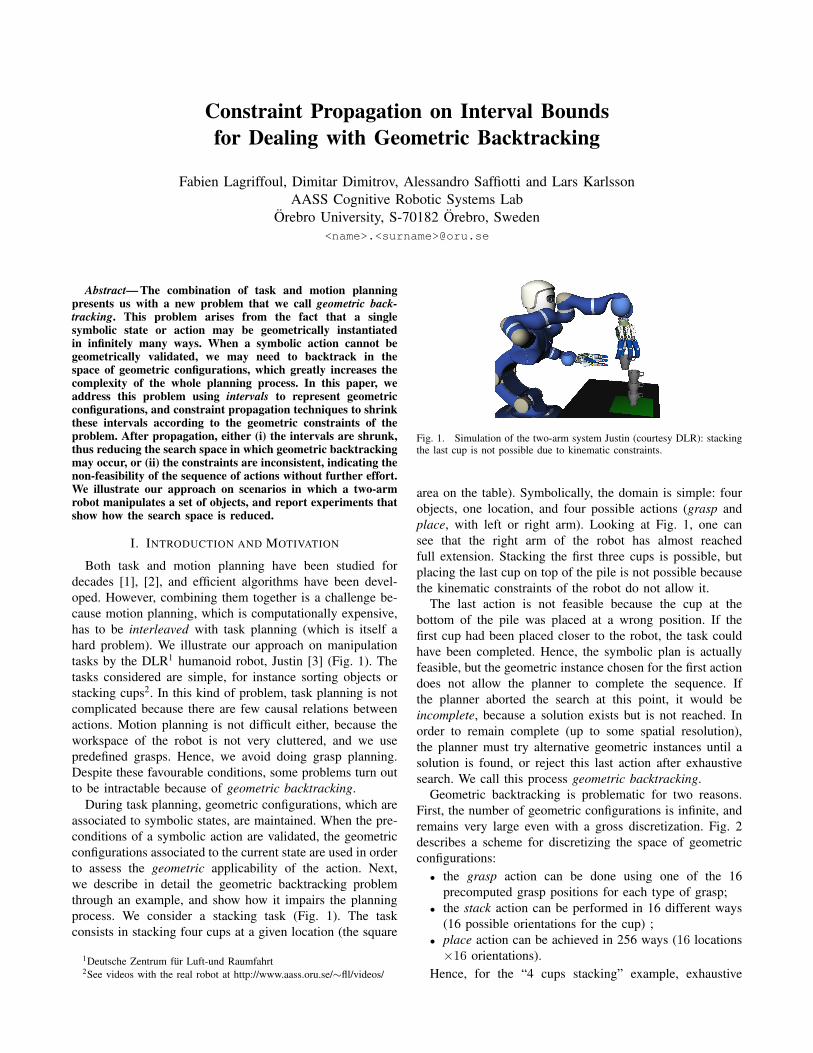
Fig. 1. Simulation of the two-arm system Justin (courtesy DLR): stackingthe last cup is not possible due to kinematic constraints.

area on the table). Symbolically, the domain is simple: fourobjects, one location, and four possible actions (grasp andplace, with left or right arm). Looking at Fig. 1, one cansee that the right arm of the robot has almost reachedfull extension. Stacking the first three cups is possible, butplacing the last cup on top of the pile is not possible becausethe kinematic constraints of the robot do not allow it.

The last action is not feasible because the cup at thebottom of the pile was placed at a wrong position. If thefirst cup had been placed closer to the robot, the task couldhave been completed. Hence, the symbolic plan is actuallyfeasible, but the geometric instance chosen for the first actiondoes not allow the planner to complete the sequence. Ifthe planner aborted the search at this point, it would beincomplete, because a solution exists but is not reached. Inorder to remain complete (up to some spatial resolution),the planner must try alternative geometric instances until asolution is found, or reject this last action after exhaustivesearch. We call this process geometric backtracking.

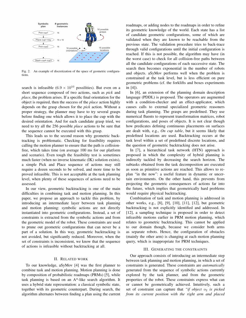
Geometric backtracking is problematic for two reasons.First, the number of geometric configurations is infinite, andremains very large even with a gross discretization. Fig. 2describes a scheme for discretizing the space of geometricconfigurations:• the grasp action can be done using one of the 16

precomputed grasp positions for each type of grasp;• the stack action can be performed in 16 different ways

(16 possible orientations for the cup) ;• place action can be achieved in 256 ways (16 locations×16 orientations).

Hence, for the “4 cups stacking” example, exhaustive

Pick cup1

Place cup1 tray

Pick cup2

Stack cup4 cup3

16 possible grasps16

16 x 16

16

16

Symbolic plan

# geometric instances

16 possible locations

16 possible orientations

Fig. 2. An example of discretization of the space of geometric configura-tions.

search is infeasible (6.9 × 1010 possilities). But even on ashort sequence composed of two actions, such as pick andplace, the problem arises. If a specific final orientation for theobject is required, then the success of the place action highlydepends on the grasp chosen for the pick action. Without aproper strategy, the planner may have to try several graspsbefore finding one which allows it to place the cup with thedesired orientation. And for each candidate grasp tried, weneed to try all the 256 possible place actions to be sure thatthe sequence cannot be executed with this grasp.

This leads us to the second reason why geometric back-tracking is problematic. Checking for feasibility requirescalling the motion planner to ensure that the path is collision-free, which takes time (on average 100 ms for our platformand scenario). Even tough the feasibility test is sometimesmuch faster (when no inverse kinematic (IK) solution exists),a simple Pick and Place sequence of actions may stillrequire a dozen seconds to be solved, and more time to beproved infeasible. This is not acceptable at the task planninglevel, when plenty of these sequences of actions need to beassessed.

In our view, geometric backtracking is one of the maindifficulties in combining task and motion planning. In thispaper, we propose an approach to tackle this problem, byintroducing an intermediate layer between task planningand motion planning: symbolic actions are not directlyinstantiated into geometric configurations. Instead, a set ofconstraints is extracted from the symbolic actions and fromthe geometric model of the robot. These constraints are usedto prune out geometric configurations that can never be apart of a solution. In this way, geometric backtracking isnot avoided, but significantly reduced. Moreover, when theset of constraints is inconsistent, we know that the sequenceof actions is infeasible without backtracking at all.

II. RELATED WORK

To our knowledge, aSyMov [4] was the first planner tocombine task and motion planning. Motion planning is doneby composition of probabilistic roadmaps (PRMs) [5], whiletask planning is based on an A*-like search algorithm. Ituses a hybrid state representation: a classical symbolic state,together with its geometric counterpart. During search, thealgorithm alternates between finding a plan using the current

roadmaps, or adding nodes to the roadmaps in order to refineits geometric knowledge of the world. Each state has a listof candidate geometric configurations, some of which arevalidated when they are known to be reachable from theprevious state. The validation procedure tries to back-tracethrough valid configurations until the initial configuration isreached. If this is not possible, the algorithm may have (inthe worst case) to check for all collision-free paths betweenall the candidate configurations of each successive state. Thesearch then becomes exponential in the number of robotsand objects. aSyMov performs well when the problem isconstrained at the task level, but is less efficient on puregeometric problems (cf. the forklifts and boxes experimentsin [4]).

In [6], an extension of the planning domain descriptionlanguage (PDDL) is proposed. The operators are augmentedwith a condition-checker and an effect-applicator, whichcauses calls to external specialized geometric reasonersduring task planning. The grasps are predefined. They usenumerical fluents to represent transformation matrices, robotconfigurations, and poses of objects. It is not clear thoughhow predicates defining continuous placements on surfacesare dealt with, e.g., On cup table, but it seems likely thatpredefined locations are used. Backtracking occurs at thetask level within a set of predefined discrete locations, andthe question of geometric backtracking does not arise.

In [7], a hierarchical task network (HTN) approach isproposed in which the complexity of hybrid planning isindirectly tackled by decreasing the search horizon. Thesubtasks obtained from the task decomposition are executedas soon as primitive actions are reached. This allows to re-plan “in the now”: a useful feature in dynamic or uncer-tain environments. On the other hand, this prevents fromprojecting the geometric consequences of actions far intothe future, which implies that geometrically hard problemswould require physical backtracking.

Combination of task and motion planning is addressed inother works, e.g., [8], [9], [10], [11], [12], but geometricbacktracking is not explicitly identified and addressed. In[12], a sampling technique is proposed in order to detectinfeasible motions earlier in PRM motion planning, whichrelates to geometric backtracking. This cannot be appliedto our domain though, because we consider both armsas separate robots. Hence, the configuration of obstacles(mainly the other arm) is changing at each motion planningquery, which is inappropriate for PRM techniques.

III. GENERATING THE CONSTRAINTS

Our approach consists of introducing an intermediate stepbetween task planning and motion planning, in which a set ofconstraints is generated. These constraints are automaticallygenerated from the sequence of symbolic actions currentlyexplored by the task planner, and from the geometricproperties of the robot. These constraints express what canor cannot be geometrically achieved. Intuitively, such aset of constraint can capture that “if object o2 is pickedfrom its current position with the right arm and placed

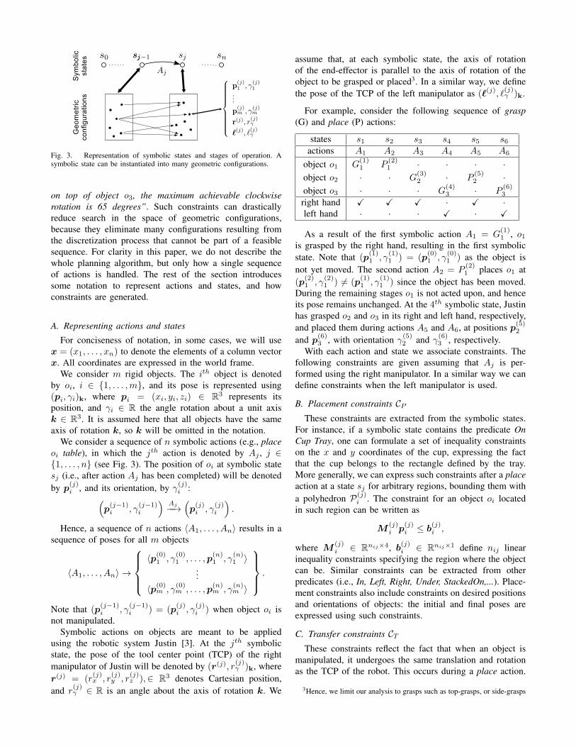
Fig. 3. Representation of symbolic states and stages of operation. Asymbolic state can be instantiated into many geometric configurations.

on top of object o3, the maximum achievable clockwiserotation is 65 degrees”. Such constraints can drasticallyreduce search in the space of geometric configurations,because they eliminate many configurations resulting fromthe discretization process that cannot be part of a feasiblesequence. For clarity in this paper, we do not describe thewhole planning algorithm, but only how a single sequenceof actions is handled. The rest of the section introducessome notation to represent actions and states, and howconstraints are generated.

A. Representing actions and states

For conciseness of notation, in some cases, we will usex = (x1, . . . , xn) to denote the elements of a column vectorx. All coordinates are expressed in the world frame.

We consider m rigid objects. The ith object is denotedby oi, i ∈ {1, . . . ,m}, and its pose is represented using(pi, γi)k, where pi = (xi, yi, zi) ∈ R3 represents itsposition, and γi ∈ R the angle rotation about a unit axisk ∈ R3. It is assumed here that all objects have the sameaxis of rotation k, so k will be omitted in the notation.

We consider a sequence of n symbolic actions (e.g., placeoi table), in which the jth action is denoted by Aj , j ∈{1, . . . , n} (see Fig. 3). The position of oi at symbolic statesj (i.e., after action Aj has been completed) will be denotedby p

(j)i , and its orientation, by γ(j)i :(

p(j−1)i , γ

(j−1)i

)Aj−−→

(p(j)i , γ

(j)i

).

Hence, a sequence of n actions 〈A1, . . . , An〉 results in asequence of poses for all m objects

〈A1, . . . , An〉 →

〈p(0)

1 , γ(0)1 , . . . ,p

(n)1 , γ

(n)1 〉

...〈p(0)m , γ

(0)m , . . . ,p

(n)m , γ

(n)m 〉

.

Note that (p(j−1)i , γ

(j−1)i ) = (p

(j)i , γ

(j)i ) when object oi is

not manipulated.Symbolic actions on objects are meant to be applied

using the robotic system Justin [3]. At the jth symbolicstate, the pose of the tool center point (TCP) of the rightmanipulator of Justin will be denoted by (r(j), r

(j)γ )k, where

r(j) = (r(j)x , r

(j)y , r

(j)z ),∈ R3 denotes Cartesian position,

and r(j)γ ∈ R is an angle about the axis of rotation k. We

assume that, at each symbolic state, the axis of rotationof the end-effector is parallel to the axis of rotation of theobject to be grasped or placed3. In a similar way, we definethe pose of the TCP of the left manipulator as (`(j), `

(j)γ )k.

For example, consider the following sequence of grasp(G) and place (P) actions:

states s1 s2 s3 s4 s5 s6actions A1 A2 A3 A4 A5 A6

object o1 G(1)1 P

(2)1 · · · ·

object o2 · · G(3)2 · P

(5)2 ·

object o3 · · · G(4)3 · P

(6)3

right hand X X X · X ·left hand · · · X · X

As a result of the first symbolic action A1 = G(1)1 , o1

is grasped by the right hand, resulting in the first symbolicstate. Note that (p

(1)1 , γ

(1)1 ) = (p

(0)1 , γ

(0)1 ) as the object is

not yet moved. The second action A2 = P(2)1 places o1 at

(p(2)1 , γ

(2)1 ) 6= (p

(1)1 , γ

(1)1 ) since the object has been moved.

During the remaining stages o1 is not acted upon, and henceits pose remains unchanged. At the 4th symbolic state, Justinhas grasped o2 and o3 in its right and left hand, respectively,and placed them during actions A5 and A6, at positions p(5)

2

and p(6)3 , with orientation γ(5)2 and γ(6)3 , respectively.

With each action and state we associate constraints. Thefollowing constraints are given assuming that Aj is per-formed using the right manipulator. In a similar way we candefine constraints when the left manipulator is used.

B. Placement constraints CPThese constraints are extracted from the symbolic states.

For instance, if a symbolic state contains the predicate OnCup Tray, one can formulate a set of inequality constraintson the x and y coordinates of the cup, expressing the factthat the cup belongs to the rectangle defined by the tray.More generally, we can express such constraints after a placeaction at a state sj for arbitrary regions, bounding them witha polyhedron P(j)

i . The constraint for an object oi locatedin such region can be written as

M(j)i p

(j)i ≤ b

(j)i ,

where M(j)i ∈ Rnij×4, b

(j)i ∈ Rnij×1 define nij linear

inequality constraints specifying the region where the objectcan be. Similar constraints can be extracted from otherpredicates (i.e., In, Left, Right, Under, StackedOn,...). Place-ment constraints also include constraints on desired positionsand orientations of objects: the initial and final poses areexpressed using such constraints.

C. Transfer constraints CTThese constraints reflect the fact that when an object is

manipulated, it undergoes the same translation and rotationas the TCP of the robot. This occurs during a place action.

3Hence, we limit our analysis to grasps such as top-grasps, or side-grasps

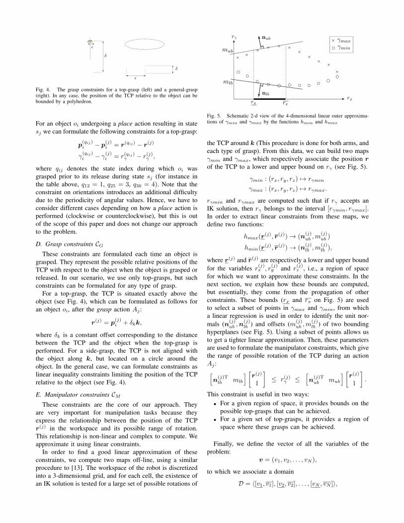
Fig. 4. The grasp constraints for a top-grasp (left) and a general-grasp(right). In any case, the position of the TCP relative to the object can bebounded by a polyhedron.

For an object oi undergoing a place action resulting in statesj we can formulate the following constraints for a top-grasp:

p(qij)i − p

(j)i = r(qij) − r(j)

γ(qij)i − γ(j)i = r(qij)γ − r(j)γ ,

where qij denotes the state index during which oi wasgrasped prior to its release during state sj (for instance inthe table above, q12 = 1, q25 = 3, q36 = 4). Note that theconstraint on orientations introduces an additional difficultydue to the periodicity of angular values. Hence, we have toconsider different cases depending on how a place action isperformed (clockwise or counterclockwise), but this is outof the scope of this paper and does not change our approachto the problem.

D. Grasp constraints CGThese constraints are formulated each time an object is

grasped. They represent the possible relative positions of theTCP with respect to the object when the object is grasped orreleased. In our scenario, we use only top-grasps, but suchconstraints can be formulated for any type of grasp.

For a top-grasp, the TCP is situated exactly above theobject (see Fig. 4), which can be formulated as follows foran object oi, after the grasp action Aj :

r(j) = p(j)i + δkk,

where δk is a constant offset corresponding to the distancebetween the TCP and the object when the top-grasp isperformed. For a side-grasp, the TCP is not aligned withthe object along k, but located on a circle around theobject. In the general case, we can formulate constraints aslinear inequality constraints limiting the position of the TCPrelative to the object (see Fig. 4).

E. Manipulator constraints CMThese constraints are the core of our approach. They

are very important for manipulation tasks because theyexpress the relationship between the position of the TCPr(j) in the workspace and its possible range of rotation.This relationship is non-linear and complex to compute. Weapproximate it using linear constraints.

In order to find a good linear approximation of theseconstraints, we compute two maps off-line, using a similarprocedure to [13]. The workspace of the robot is discretizedinto a 3-dimensional grid, and for each cell, the existence ofan IK solution is tested for a large set of possible rotations of

Fig. 5. Schematic 2-d view of the 4-dimensional linear outer approxima-tions of γmin and γmax by the functions hmin and hmax

the TCP around k (This procedure is done for both arms, andeach type of grasp). From this data, we can build two mapsγmin and γmax, which respectively associate the position rof the TCP to a lower and upper bound on rγ (see Fig. 5).

γmin : (rx, ry, rz) 7→ rγmin

γmax : (rx, ry, rz) 7→ rγmax.

rγmin and rγmax are computed such that if rγ accepts anIK solution, then rγ belongs to the interval [rγmin, rγmax].In order to extract linear constraints from these maps, wedefine two functions:

hmax(r(j), r(j))→ (n

(j)ub ,m

(j)ub )

hmin(r(j), r(j))→ (n

(j)lb ,m

(j)lb ),

where r(j) and r(j) are respectively a lower and upper boundfor the variables r(j)x , r

(j)y and r

(j)z , i.e., a region of space

for which we want to approximate these constraints. In thenext section, we explain how these bounds are computed,but essentially, they come from the propagation of otherconstraints. These bounds (rx and rx on Fig. 5) are usedto select a subset of points in γmax and γmin, from whicha linear regression is used in order to identify the unit nor-mals (n(j)

ub ,n(j)lb ) and offsets (m(j)

ub ,m(j)lb ) of two bounding

hyperplanes (see Fig. 5). Using a subset of points allows usto get a tighter linear approximation. Then, these parametersare used to formulate the manipulator constraints, which givethe range of possible rotation of the TCP during an actionAj :[n

(j)Tlb mlb

] [r(j)

1

]≤ r(j)γ ≤

[n

(j)Tub mub

] [r(j)

1

].

This constraint is useful in two ways:• For a given region of space, it provides bounds on the

possible top-grasps that can be achieved.• For a given set of top-grasps, it provides a region of

space where these grasps can be achieved.

Finally, we define the vector of all the variables of theproblem:

v = (v1, v2, . . . , vN ),

to which we associate a domain

D = 〈[v1, v1], [v2, v2], . . . , [vN , vN ]〉,

where each variable vi has associated bounds [vi, vi]. Theset of all constraints of the problem

C = {C(j)P , C(j)T , C(j)G , C(j)M }, j ∈ {1, . . . , n}

can be expressed as

Pv ≤ d (1)Qv = e, (2)

where (1) and (2) represent respectively the inequality andequality constraints of our problem. In addition, we definea geometric configuration (see Fig. 3) as a set of valuesrepresenting the poses of all objects, and the poses of bothTCPs:

c = {p1, . . . ,pm, r, `}. (3)

IV. USING CONSTRAINTS TO COMPUTE INTERVALS

The geometric constraints of the problem are formulatedwith a set of linear inequalities (1) and equalities (2).The manipulator constraints CM have been formulated interms of lower and upper bounds on the actual capabilitiesof the manipulator. Consequently, the set of constraints isconservative, i.e., if a solution exists, it must belong to thefeasible set defined by the constraints (conversely, if theconstraints result in an empty feasible set, the problem hasno solution). Note, however, that• we still have to search the feasible set for a sequence

of configurations which solves the problem;• we still have to do motion planning to find collision-free

paths connecting grasp and release positions.For these reasons, instead of searching for a single solution,we use the constraints to tighten the bounds of a set ofintervals which contain all the solutions to the problem.

A. Narrowing intervals

Algorithm 1: FilterDomain

Function FilterDomain(D, C)input : D: a domain

C: a set of linear constraints

1 ε = minimal domain reduction

2 D′ = D3 repeat4 D = D′

5 UpdateManipulatorConstraints(C,D)6 for i← 1 to N do7 minimize

vvi, subject to Pv ≤ d,Qv = e

8 vi′ ← max(vi, v

?i )

9 maximizev

vi, subject to Pv ≤ d,Qv = e

10 vi′ ← min(vi, v

?i )

11 until Dist(D,D′) ≤ ε or D′ = ∅12 return D′

The bounds of the intervals are computed using Algorithm1, a global filtering algorithm (adapted from [14]) which

converges rapidly and detects inconsistency at the first it-eration. This algorithm solves several linear programs (LP)in order to find the minimum (resp. maximum) value v?iof each variable vi. v?i is then used to update the lower(resp. upper) bound of vi (lines 8 and 10). The valuesare updated in a temporary copy of the domain D′ =〈[v1′, v1′], [v2′, v2′], . . . , [vN ′, vN ′]〉, which is used in orderto measure how much the intervals have shrunk after eachiteration. This is done by the Dist function (line 11), whichreturns the average of the differences between upper andlower bounds in D and D′. The process is repeated until thedomains do not change more than a predefined ε value. Theresult is a domain in which the intervals are narrowed withrespect to the constraints, or ∅ if an inconsistency is detectedduring the resolution of a LP.

We have modified the original algorithm by adding thefunction UpdateManipulatorConstraints(C,D) in themain loop (line 5). Indeed, after each iteration, the intervalsmay shrink. If the intervals representing the TCP positionsare reduced, it is meaningful to refine the manipulatorconstraints using the functions hmin and hmax in order toget a tighter linear approximation of the real problem.

Refining the manipulator constraints while filtering thedomains is a very efficient process. Let us illustrate this witha numerical example for a pick action. Initially, the problemconsists of four variables representing the position of theobject “cup” located at (0.6, 0.25, 0.1) with orientation 0.

v = (x(0)cup, y(0)cup, z

(0)cup, γ

(0)cup)

D = 〈[0.6, 0.6], [0.25, 0.25], [0.1, 0.1], [0, 0]〉.

The lower bounds are equal to the upper bounds because thevalues of the variables are determined. The pick action leadsus to the creation of 4 new variables for the TCP, which areinitially assigned arbitrarily large intervals:

v = (x(0)cup, y(0)cup, z

(0)cup, γ

(0)cup, r

(1)x , r(1)y , r(1)z , r(1)γ )

D = 〈[0.6, 0.6], [0.25, 0.25], [0.10, 0.10], [0, 0],

[−10, 10], [−10, 10], [−10, 10], [−π, π]〉.

A pick action also generates grasp constraints CG and manip-ulator constraints CM . We use k = (0, 0, 1) and δk = 0.34:

r(1)x = x(0)cup

r(1)y = y(0)cup − 0.70 ≤ rγ ≤ 2.36

r(1)z = z(0)cup + 0.34 (using hmin and hmax).

After applying the function FilterDomain, D becomes:

D = 〈[0.6, 0.6], [0.25, 0.25], [0.10, 0.10], [0, 0],

[0.6, 0.6], [0.25, 0.25], [0.44, 0.44], [−0.70, 2.36]〉.

The grasp constraints have propagated the values of theposition of the cup to the position of the TCP. In the seconditeration, the bounds on the orientation of the TCP r(1)γ havebeen updated with the linear approximations of the maps,but since the domain of the TCP is now a single point, thesebounds represent the possible rotation of the TCP at this

point. Hence, in order to pick the cup, the orientation of thetop-grasp must be chosen between −0.70 and 2.36 radians.

This constraint propagation process is interesting forlonger sequences of actions, because it allows us to propagatethe consequences of early choices until the final actions. Itcould for instance solve the stacking problem described inthe introduction, and even give an approximation of a regionon the table which is appropriate for placing the first cup.

B. Narrowing intervals during search

In order to find a solution, we use a basic depth-first-search algorithm, endowed with a pruning step (see algo-rithm 2: SearchAndFilter (SAF)). Geometric instances ofconfigurations are not chosen arbitrarily, but such that thevariables representing them (see definition (3)) belong totheir respective intervals. This is the first level of pruning.But after an action has been chosen (e.g., to place the cupat position (0.7,−0.25, 0.1) with γ = π/2), the variablesrepresenting this choice are assigned fixed values, so thecorresponding intervals can be reduced to single points (i.e.,for a variable vi, vi = vi). Then, we can filter the domainagain in order to propagate this choice to other variablesthrough the constraints. The other intervals will be shrunkaccordingly, which will reduce even more the possibilitiesfor further actions. This process is repeated each time anaction is chosen, so that intervals are shrunk as the searchprogresses.

Algorithm 2: SearchAndFilter

Function SearchAndFilter(c1, Seq,D)input : c1: a geometric configuration

Seq: a sequence of symbolic actionsD: a domain

1 if Seq = 〈〉 then return c12 Action = Seq.head3 Rest = Seq.tail

4 foreach Ai ∈ geometricInstanceOf (Action) do5 c2 = getSuccesorConf(c1, Ai)

6 if c2 ∈ D then7 D′ = assignV alues(D, c2)8 D′ = filterDomain(D′)

9 if D′ 6= ∅ then10 feasible = pathP lanning(c1, c2)

11 if feasible then12 s = SearchAndFilter(c2, Rest,D′)13 if s 6= false then14 return 〈c2, s〉

15 return false

Algorithm 2 is initially called with the initial geometricconfiguration, the sequence of symbolic actions, and theinitial domain filtered according to the constraints of theproblem. An action Ai is chosen among the possible geo-metric instances of Action (e.g., 16 for Pick, 256 for Place).

c2 is the result of applying Ai to c1. If this configurationbelongs to the domain, we apply the strategy describedabove, that assigns the values to the domain and filters itagain (lines 7-8). If no inconsistency appears, the motionplanning algorithm is called to check if a collision-free pathexists to reach c2. If a path exists, the function is recursivelycalled on c2 with the remaining actions and the shrunkdomain D′, otherwise the next action Ai is tried. If all theactions fail, the function returns false to the calling functionvia the return statement line 15. If a final configuration isreached (line 1), the solution is incrementally built (line 14)and returned to the main calling function. The result is alist of geometric configurations and paths which are used toexecute the final plan (paths are smoothed after a plan isfound, see end of section V.A).

C. Detecting inconsistency and pruning

One of the main problems of geometric backtrackingis when no geometric instantiation of the action sequenceexists. This happens often during task planning, because nogeometric information is used. For instance, the task plannermay try a sequence in which the right arm of the robot graspsan object situated on the left side. In the worst case, forsuch a sequence, all the space of configurations has to besearched in order to discover that it is infeasible, which maybe computationally expensive. The only solution to avoidthis is to impose a time limit on the backtracking process.Unfortunately by doing this, completeness is lost for caseswhen the problem is feasible.

On the other hand in our approach, inconsistency can bedetected before entering the backtracking procedure, whilewe filter the initial domain according to the constraints of theproblem. This is more efficient since no search is required.Inconsistency can also be exploited during search in orderto prune out a whole branch of the search tree. This happenswhen the problem is initially consistent, and at some pointin the search, an action is chosen that makes the probleminconsistent. This will be detected during filtering (line 8-9in the Algorithm 2). Then, we do not need to search furtherwith this action sequence, and can try another action.

V. EXPERIMENTAL RESULTS

A. Experimental setup

Geometric backtracking might occur while evaluating thefeasibility of a sequence of symbolic actions. What a taskplanner does is essentially to evaluate many of these se-quences. Hence, we evaluated our approach by evaluatingsingle sequences of actions. We compare our algorithm SAFto a standard depth-first-search (DFS) procedure, i.e., SAFwithout the filtering process (lines 6 to 9), and without usingthe argument D′ at line 12. We compare our algorithmagainst DFS, because DFS is equivalent to the strategiesused in similar work (see Section II), i.e., a non-informedbacktracking search.

We use a simulation environment provided by DLR forthe robotic platform Justin [3]. Simulation is more suitedfor this kind of experiments, but similar tasks have been

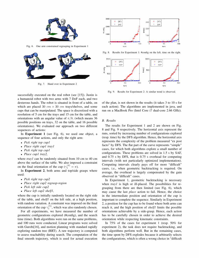
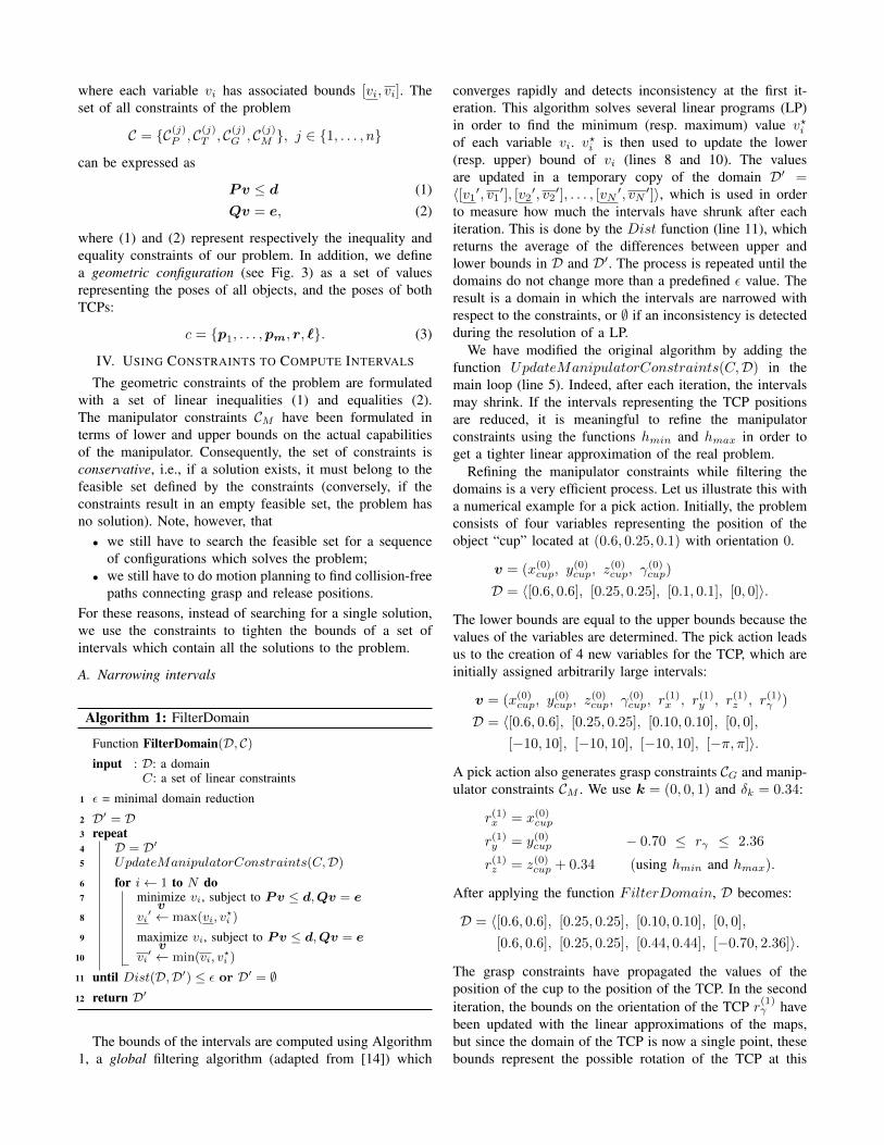
Fig. 6. One arm constrained regrasping in Experiment 1

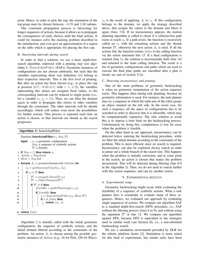
Fig. 7. Hand over in Experiment 2

successfully executed on the real robot (see [15]). Justin isa humanoid robot with two arms with 7 DoF each, and twodexterous hands. The robot is situated in front of a table, onwhich are placed 30 cm × 30 cm trays/shelves, and somecups that can be manipulated. The space is discretized with aresolution of 5 cm for the trays and 15 cm for the table, andorientations with an angular value of π/8. (which means 36possible positions on trays, 32 on the table, and 16 possibleorientations). We evaluated our approach on two differentsequences of actions:

In Experiment 1 (see Fig. 6), we used one object, asequence of four actions, and only the right arm:• Pick right top cup1• Place right cup1 tray1• Pick right top cup1• Place cup1 tray2,

where tray1 can be randomly situated from 10 cm to 40 cmabove the surface of the table. We also imposed a constrainton the final orientation of the cup (γ(4)1 = π).

In Experiment 2, both arms and top/side grasps whereused:• Pick right top cup2• Place right cup2 regrasp-region• Pick left side cup2• Place left cup2 shelf1,

where the cup is initially randomly located on the right sideof the table, and shelf1 on the left side, at a high position,with random variation. A constraint was imposed on the finalorientation of the cup γ(5)1 , which was also randomly chosen.

For all experiments, we have measured the number ofgeometric configurations explored (#config), and the searchtime (time). Both algorithms were run on the same problems,and 100 runs were conducted. Linear programs were solvedwith Gurobi[16], and motion planning with standard rapidlyexploring random tree (RRT). A raw trajectory is computedto assess reachability during search. The computation of thefinal smooth trajectory, which is used for actual execution

Fig. 8. Results for Experiment 1: #config on the left, time on the right.

Fig. 9. Results for Experiment 2: A similar trend is observed.

of the plan, is not shown in the results (it takes 3 to 10 s foreach action). The algorithms are implemented in java, andrun on a MacBook Pro (Intel Core i7 dual-core 2.66 GHz).

B. Results

The results for Experiment 1 and 2 are shown on Fig.8 and Fig. 9 respectively. The horizontal axis represent theruns, sorted by increasing number of configurations explored(resp. time) by the DFS algorithm. Hence, the horizontal axisrepresents the complexity of the problem measured “ex postfacto” by DFS. The flat part of the curve represents “simple”cases, for which both algorithms explore a small number ofconfigurations. These problems are solved in 1.5 s by SAF,and 0.75 s by DFS, that is 0.75 s overhead for computingintervals (with not particularly optimized implementation).Computing intervals clearly pays off for more “difficult”cases, i.e., when geometric backtracking is required. Onaverage, the overhead is largely compensated by the gainobserved in “difficult” cases.

In Experiment 1, geometric backtracking is necessarywhen tray1 is high or ill-placed. The possibilities for re-grasping from there are then limited (see Fig. 6), whichmay cause the last place action to fail. Hence, the choicein the intermediate position and orientation of the cup isimportant to complete the sequence. Similarly in Experiment2, a position for the cup has to be found where both arms canreach it, and the high position of shelf1 limits the possibleorientations achievable by a side-grasp. Hence, each actionhas to be carefully chosen in order to achieve the desiredorientation while respecting kinematic constraints.

In 75% of the cases for experiment 1 (resp. 50% forexperiment 2), the task does not require backtracking, andboth algorithms perform well. But in the remaining cases,the time spent by DFS explodes because it arbitrarily selectsthe configurations, which is often a wrong choice in “difficult

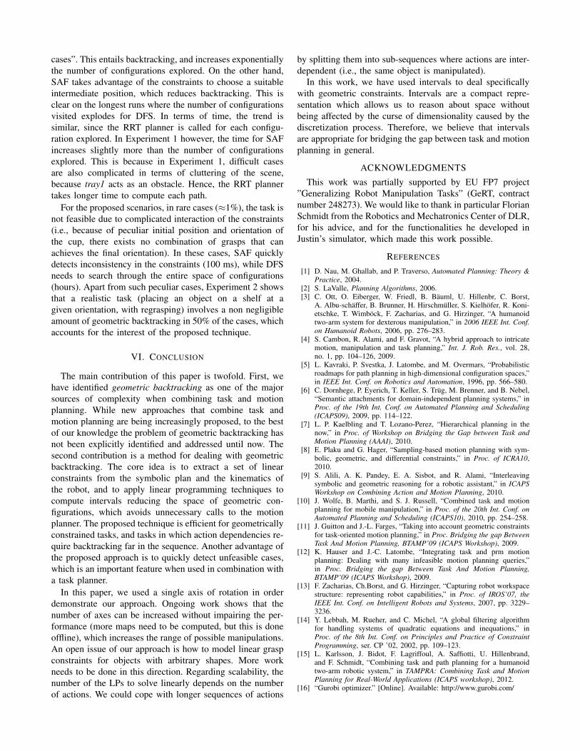
cases”. This entails backtracking, and increases exponentiallythe number of configurations explored. On the other hand,SAF takes advantage of the constraints to choose a suitableintermediate position, which reduces backtracking. This isclear on the longest runs where the number of configurationsvisited explodes for DFS. In terms of time, the trend issimilar, since the RRT planner is called for each configu-ration explored. In Experiment 1 however, the time for SAFincreases slightly more than the number of configurationsexplored. This is because in Experiment 1, difficult casesare also complicated in terms of cluttering of the scene,because tray1 acts as an obstacle. Hence, the RRT plannertakes longer time to compute each path.

For the proposed scenarios, in rare cases (≈1%), the task isnot feasible due to complicated interaction of the constraints(i.e., because of peculiar initial position and orientation ofthe cup, there exists no combination of grasps that canachieves the final orientation). In these cases, SAF quicklydetects inconsistency in the constraints (100 ms), while DFSneeds to search through the entire space of configurations(hours). Apart from such peculiar cases, Experiment 2 showsthat a realistic task (placing an object on a shelf at agiven orientation, with regrasping) involves a non negligibleamount of geometric backtracking in 50% of the cases, whichaccounts for the interest of the proposed technique.

VI. CONCLUSION

The main contribution of this paper is twofold. First, wehave identified geometric backtracking as one of the majorsources of complexity when combining task and motionplanning. While new approaches that combine task andmotion planning are being increasingly proposed, to the bestof our knowledge the problem of geometric backtracking hasnot been explicitly identified and addressed until now. Thesecond contribution is a method for dealing with geometricbacktracking. The core idea is to extract a set of linearconstraints from the symbolic plan and the kinematics ofthe robot, and to apply linear programming techniques tocompute intervals reducing the space of geometric con-figurations, which avoids unnecessary calls to the motionplanner. The proposed technique is efficient for geometricallyconstrained tasks, and tasks in which action dependencies re-quire backtracking far in the sequence. Another advantage ofthe proposed approach is to quickly detect unfeasible cases,which is an important feature when used in combination witha task planner.

In this paper, we used a single axis of rotation in orderdemonstrate our approach. Ongoing work shows that thenumber of axes can be increased without impairing the per-formance (more maps need to be computed, but this is doneoffline), which increases the range of possible manipulations.An open issue of our approach is how to model linear graspconstraints for objects with arbitrary shapes. More workneeds to be done in this direction. Regarding scalability, thenumber of the LPs to solve linearly depends on the numberof actions. We could cope with longer sequences of actions

by splitting them into sub-sequences where actions are inter-dependent (i.e., the same object is manipulated).

In this work, we have used intervals to deal specificallywith geometric constraints. Intervals are a compact repre-sentation which allows us to reason about space withoutbeing affected by the curse of dimensionality caused by thediscretization process. Therefore, we believe that intervalsare appropriate for bridging the gap between task and motionplanning in general.

ACKNOWLEDGMENTS

This work was partially supported by EU FP7 project”Generalizing Robot Manipulation Tasks” (GeRT, contractnumber 248273). We would like to thank in particular FlorianSchmidt from the Robotics and Mechatronics Center of DLR,for his advice, and for the functionalities he developed inJustin’s simulator, which made this work possible.

REFERENCES

[1] D. Nau, M. Ghallab, and P. Traverso, Automated Planning: Theory &Practice, 2004.

[2] S. LaValle, Planning Algorithms, 2006.[3] C. Ott, O. Eiberger, W. Friedl, B. Bauml, U. Hillenbr, C. Borst,

A. Albu-schaffer, B. Brunner, H. Hirschmuller, S. Kielhofer, R. Koni-etschke, T. Wimbock, F. Zacharias, and G. Hirzinger, “A humanoidtwo-arm system for dexterous manipulation,” in 2006 IEEE Int. Conf.on Humanoid Robots, 2006, pp. 276–283.

[4] S. Cambon, R. Alami, and F. Gravot, “A hybrid approach to intricatemotion, manipulation and task planning,” Int. J. Rob. Res., vol. 28,no. 1, pp. 104–126, 2009.

[5] L. Kavraki, P. Svestka, J. Latombe, and M. Overmars, “Probabilisticroadmaps for path planning in high-dimensional configuration spaces,”in IEEE Int. Conf. on Robotics and Automation, 1996, pp. 566–580.

[6] C. Dornhege, P. Eyerich, T. Keller, S. Trug, M. Brenner, and B. Nebel,“Semantic attachments for domain-independent planning systems,” inProc. of the 19th Int. Conf. on Automated Planning and Scheduling(ICAPS09), 2009, pp. 114–122.

[7] L. P. Kaelbling and T. Lozano-Perez, “Hierarchical planning in thenow,” in Proc. of Workshop on Bridging the Gap between Task andMotion Planning (AAAI), 2010.

[8] E. Plaku and G. Hager, “Sampling-based motion planning with sym-bolic, geometric, and differential constraints,” in Proc. of ICRA10,2010.

[9] S. Alili, A. K. Pandey, E. A. Sisbot, and R. Alami, “Interleavingsymbolic and geometric reasoning for a robotic assistant,” in ICAPSWorkshop on Combining Action and Motion Planning, 2010.

[10] J. Wolfe, B. Marthi, and S. J. Russell, “Combined task and motionplanning for mobile manipulation,” in Proc. of the 20th Int. Conf. onAutomated Planning and Scheduling (ICAPS10), 2010, pp. 254–258.

[11] J. Guitton and J.-L. Farges, “Taking into account geometric constraintsfor task-oriented motion planning,” in Proc. Bridging the gap BetweenTask And Motion Planning, BTAMP’09 (ICAPS Workshop), 2009.

[12] K. Hauser and J.-C. Latombe, “Integrating task and prm motionplanning: Dealing with many infeasible motion planning queries,”in Proc. Bridging the gap Between Task And Motion Planning,BTAMP’09 (ICAPS Workshop), 2009.

[13] F. Zacharias, Ch.Borst, and G. Hirzinger, “Capturing robot workspacestructure: representing robot capabilities,” in Proc. of IROS’07, theIEEE Int. Conf. on Intelligent Robots and Systems, 2007, pp. 3229–3236.

[14] Y. Lebbah, M. Rueher, and C. Michel, “A global filtering algorithmfor handling systems of quadratic equations and inequations,” inProc. of the 8th Int. Conf. on Principles and Practice of ConstraintProgramming, ser. CP ’02, 2002, pp. 109–123.

[15] L. Karlsson, J. Bidot, F. Lagriffoul, A. Saffiotti, U. Hillenbrand,and F. Schmidt, “Combining task and path planning for a humanoidtwo-arm robotic system,” in TAMPRA: Combining Task and MotionPlanning for Real-World Applications (ICAPS workshop), 2012.

[16] “Gurobi optimizer.” [Online]. Available: http://www.gurobi.com/