15 lower bounds - courses

15

Lower Bounds

How do I know if I have a good algorithm to solve a problem? If my algorithm runsin Θ(n log n) time, is that good? It would be if I were sorting the records storedin an array. But it would be terrible if I were searching the array for the largestelement. The value of an algorithm must be determined in relation to the inherentcomplexity of the algorithm at hand.

In Section 3.6 we defined the upper bound for a problem to be the upper boundof the best algorithm we know for that problem, and the lower bound to be thetightest lower bound that we can prove over all algorithms for that problem. Whilewe usually can recognize the upper bound for a given algorithm, finding the tightestlower bound for all possible algorithms is often difficult, especially if that lowerbound is more than the “trivial” lower bound determined by measuring the amountof input that must be processed.

The benefits of being able to discover a strong lower bound are significant. Inparticular, when we can make the upper and lower bounds for a problem meet,this means that we truely understand our problem in a theoretical sense. It alsosaves us the effort of attempting to discover more efficient algorithms when nosuch algorithm can exist.

Often the most effective way to determine the lower bound for a problem is tofind a reduction to another problem whose lower bound is already known. This wasthe subject of Chapter 17. However, this approach does not help us when we cannotfind a suitable “similar problem.” We focus on this chapter with discovering andproving lower bounds from first principles. A significant example of a lower boundsargument is the proof from Section 7.9 that the problem of sorting is O(n log n) inthe worst case.

Section 15.1 reviews the concept of a lower bound for a problem and presentsa basic “algorithm” for finding a good algorithm. Section 15.2 discusses lower

511

512 Chap. 15 Lower Bounds

bounds on searching in lists, both those that are unordered and those that are or-dered. Section 15.3 deals with finding the maximum value in a list, and presents amodel for selection based on building a partially ordered set. Section 15.4 presentsthe concept of an adversarial lower bounds proof. Section 15.5 illustrates the con-cept of a state space lower bound. Section 15.6 presents a linear time worst-casealgorithm for finding the ith biggest element on a list. Section 15.7 continues ourdiscussion of sorting with a search for an algorithm that requires the absolute fewestnumber of comparisons needed to sort a list.

15.1 Introduction to Lower Bounds Proofs

The lower bound for the problem is the tightest (highest) lower bound that wecan prove for all possible algorithms.1 This can be difficult bar, given that wecannot possibly know all algorithms for any problem, since there are theoreticallyan infinite number. However, we can often recognize a simple lower bound basedon the amount of input that must be examined. For example, we can argue that thelower bound for any algorithm to find the maximum-valued element in an unsortedlist must be Ω(n) because any algorithm must examine all of the inputs to be surethat it actually finds the maximum value.

In the case of maximum finding, the fact that we know of a simple algorithmthat runs in O(n) time, combined with the fact that any algorithm needs Ω(n) time,is significant. Since our upper and lower bounds meet (within a constant factor),we know that we do have a “good” algorithm for solving the problem. It is possiblethat someone can develop an implementation that is a “little” faster than an existingone, by a constant factor. But we know that its not possible to develop one that isasymptotically better.

So now we have an answer to the question “How do I know if I have a goodalgorithm to solve a problem?” An algorithm is good (asymptotically speaking) ifits upper bound matches the problem’s lower bound. If they match, we know to stoptrying to find an (asymptotically) faster algorithm. The problem comes when the(known) upper bound for our algorithm does not match the (known) lower boundfor the problem. In this case, we might not know what to do. Is our upper boundflawed, and the algorithm is really faster than we can prove? Is our lower boundweak, and the true lower bound for the problem is greater? Or is our algorithmsimply not the best?

1Throughout this discussion, it should be understood that any mention of bounds must specifywhat class of inputs are being considered. Do we mean the bound for the worst case input? Theaverage cost over all inputs? However, regardless of which class of inputs we consider, all of theissues raised apply equally.

Sec. 15.1 Introduction to Lower Bounds Proofs 513

Now we know precisely what we are aiming for when designing an algorithm:We want to find an algorithm who’s upper bound matches the lower bound of theproblem. Putting together all that we know so far about algorithms, we can organizeour thinking into the following “algorithm for designing algorithms.”2

If the upper and lower bounds match,then stop,else if the bounds are close or the problem isn’t important,

then stop,else if the problem definition focuses on the wrong thing,

then restate it,else if the algorithm is too slow,

then find a faster algorithm,else if lower bound is too weak,

then generate stronger bound.

We can repeat this process until we are satisfied or exhausted.This brings us smack up against one of the toughest tasks in analysis. Lower

bounds proofs are notoriously difficult to construct. The problem is coming up witharguments that truly cover all of the things that any algorithm possibly could do.The most common fallicy is to argue from the point of view of what some goodalgorithm actually does do, and claim that any algorithm must do the same. Thissimply is not true, and any lower bounds proof that refers to any specific behaviorthat must take place should be viewed with some suspicion.

Let us consider the Towers of Hanoi problem again. Recall from Section 2.5that our basic algorithm is to move n − 1 disks (recursively) to the middle pole,move the bottom disk to the third pole, and then move n−1 disks (again recursively)from the middle to the third pole. This algorithm generates the recurrance T(n) =2T(n− 1) + 1 = 2n − 1. So, the upper bound for our algorithm is 2n − 1. But isthis the best algorithm for the problem? What is the lower bound for the problem?

For our first try at a lower bounds proof, the “trivial” lower bound is that wemust move every disk at least once, for a minimum cost of n. Slightly better is toobserve that to get the bottom disk to the third pole, we must move every other diskat least twice (once to get them off the bottom disk, and once to get them over tothe third pole). This yields a cost of 2n− 1, which still is not a good match for ouralgorithm. Is the problem in the algorithm or in the lower bound?

We can get to the correct lower bound by the following reasoning: To move thebiggest disk from first to the last pole, we must first have all of the other n−1 disks

2I give credit to Gregory J.E. Rawlins for presenting this formulation in his book “Compared toWhat?”


out of the way, and the only way to do that is to move them all to the middle pole(for a cost of at least T(n− 1)). We then must move the bottom disk (for a cost ofat least one). After that, we must move the n− 1 remaining disks from the middlepole to the third pole (for a cost of at least T(n− 1)). Thus, no possible algorithmcan solve the problem in less than 2n − 1 steps. Thus, our algorithm is optimal.3

Of course, there are variations to a given problem. Changes in the problemdefinition might or might not lead to changes in the lower bound. Two examplechanges to the standard Towers of Hanoi problem are:

• Not all disks need to start on the first pole.• Multiple disks can be moved at one time.

The first variation does not affect the lower bound (at least not asymptotically). Thesecond one does.

15.2 Lower Bounds on Searching Lists

In Section 7.9 we presented an important lower bounds proof to show that theproblem of sorting is Θ(n log n) in the worst case. In Chapter 9 we discussed anumber of algorithms to search in sorted and unsorted lists, but we did not provideany lower bounds proofs to this imporant problem. We will extend our pool oftechniques for lower bounds proofs in this section by studying lower bounds forsearching unsorted and sorted lists.

15.2.1 Searching in Unsorted Lists

Given an (unsorted) list L of n elements and a search key K, we seek to identify oneelement in L which has key value K, if any exist. For the rest of this discussion, wewill assume that the key values for the elements in L are unique, that the set of allpossible keys is totally ordered (that is, the operations <, =, and > are all defined),and that comparison is our only way to find the relative ordering of two keys. Ourgoal is to solve the problem using the minimum number of comparisons.

Given this definition for searching, we can easily come up with the standardsequential search algorithm, and we can also see that the lower bound for this prob-lem is “obviously” n comparisons. (Keep in mind that the key K might not actuallyappear in the list.) However, lower bounds proofs are a bit slippery, and it is in-structive to see how they can go wrong.

3Recalling the advice to be suspicious of any lower bounds proof that argues a given behavior“must” happen, this proof should be raising red flags. However, in this particular case the problem isso constrained that there really is no alternative to this particular sequence of events.

Sec. 15.2 Lower Bounds on Searching Lists 515

Theorem 15.1 The lower bound for the problem of searching in an unsorted listis n comparisons.

Here is our first attempt at proving the theorem.Proof: Lets try a proof by contradiction. Assume an algorithm A exists that re-quires only n− 1 (or less) comparisons of K with elements of L. Since there are nelements of L, A must have avoided comparing K with L[i] for some value i. Wecan feed the algorithm an input with K in position i. Such an input is legal in ourmodel, so the algorithm is incorrect. 2

Is this proof correct? Unfortunately no. First of all, any given algorithm neednot necessarily consistently skip any given position i in its n − 1 searches. Forexample, it is not necessary that all algorithms search the list from left to right. Itis not even necessary that all algorithms search the same n− 1 positions first eachtime through the list.

We can try to dress up the proof as follows: On any given run of the algorithm,some element i gets skipped. It is possible that K is in position i at that time, andwill not be found.

Unfortunately, there is another error that needs to be fixed. It is not true that allalgorithms for solving the problem must work by comparing elements of L againstK. An algorithm might make useful progress by comparing elements of L againsteach other. For example, if we compare two elements of L, then compare thegreater against K and find that it is less than K, we know that the other element isalso less than K. It seems intuitively obvious that such comparisons won’t actuallylead to a faster algorithm, but how do we know for sure? We somehow need togeneralize the proof to account for this approach.

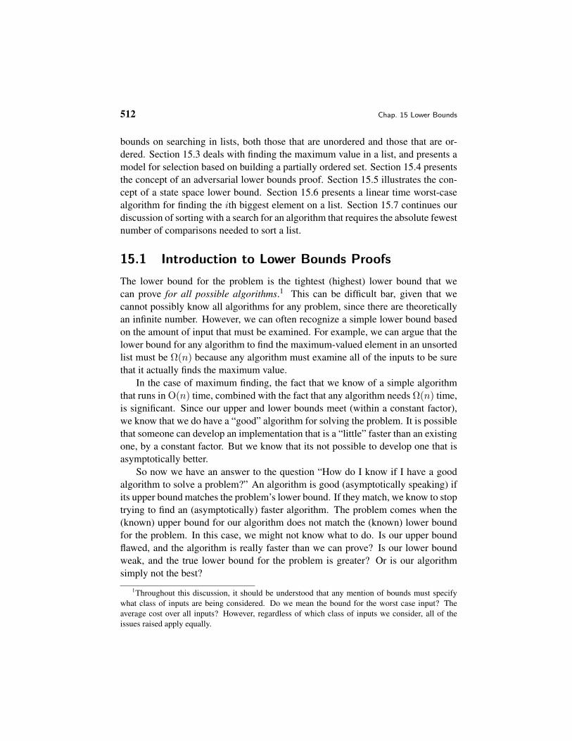
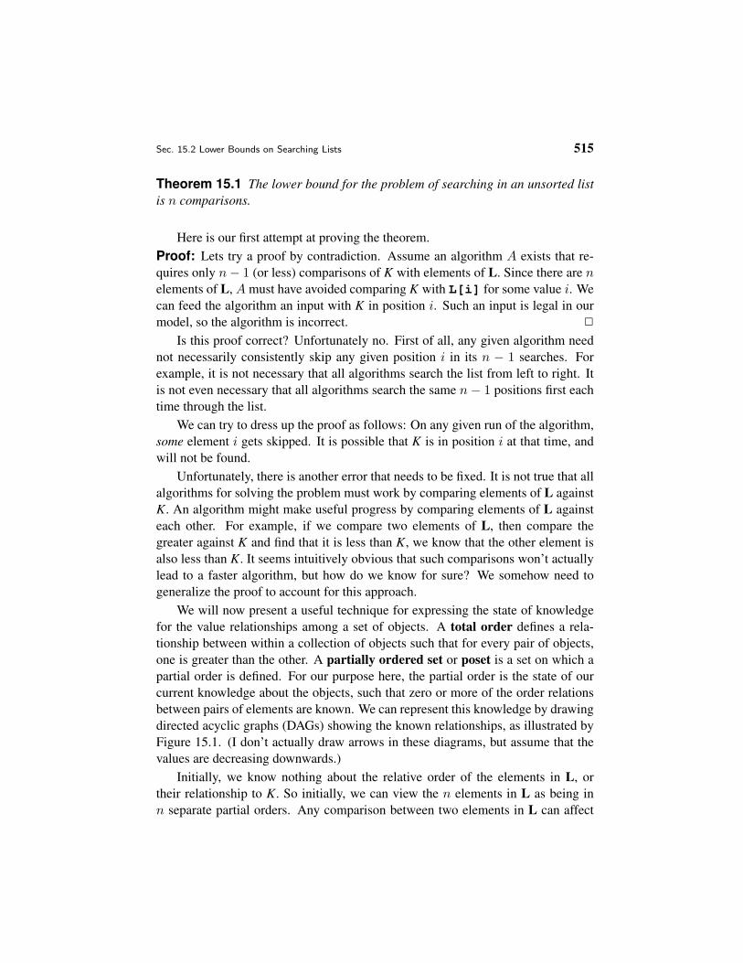
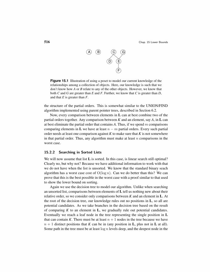
We will now present a useful technique for expressing the state of knowledgefor the value relationships among a set of objects. A total order defines a rela-tionship between within a collection of objects such that for every pair of objects,one is greater than the other. A partially ordered set or poset is a set on which apartial order is defined. For our purpose here, the partial order is the state of ourcurrent knowledge about the objects, such that zero or more of the order relationsbetween pairs of elements are known. We can represent this knowledge by drawingdirected acyclic graphs (DAGs) showing the known relationships, as illustrated byFigure 15.1. (I don’t actually draw arrows in these diagrams, but assume that thevalues are decreasing downwards.)

Initially, we know nothing about the relative order of the elements in L, ortheir relationship to K. So initially, we can view the n elements in L as being inn separate partial orders. Any comparison between two elements in L can affect


A

F

B

D

C

E

G

Figure 15.1 Illustration of using a poset to model our current knowledge of therelationships among a collection of objects. Here, our knowledge is such that wedon’t know how A or B relate to any of the other objects. However, we know thatboth C and G are greater than E and F. Further, we know that C is greater than D,and that E is greater than F.

the structure of the partial orders. This is somewhat similar to the UNION/FINDalgorithm implemented using parent pointer trees, described in Section 6.2.

Now, every comparison between elements in L can at best combine two of thepartial orders together. Any comparison between K and an element, say A, in L canat best eliminate the partial order that contains A. Thus, if we spend m comparisonscomparing elements in L we have at least n−m partial orders. Every such partialorder needs at least one comparison against K to make sure that K is not somewherein that partial order. Thus, any algorithm must make at least n comparisons in theworst case.

15.2.2 Searching in Sorted Lists

We will now assume that list L is sorted. In this case, is linear search still optimal?Clearly no, but why not? Because we have additional information to work with thatwe do not have when the list is unsorted. We know that the standard binary seachalgorithm has a worst case cost of O(log n). Can we do better than this? We canprove that this is the best possible in the worst case with a proof similar to that usedto show the lower bound on sorting.

Again we use the decision tree to model our algorithm. Unlike when searchingan unsorted list, comparisons between elements of L tell us nothing new about theirrelative order, so we consider only comparisons between K and an element in L. Atthe root of the decision tree, our knowledge rules out no positions in L, so all arepotential candidates. As we take branches in the decision tree based on the resultof comparing K to an element in L, we gradually rule out potential candidates.Eventually we reach a leaf node in the tree representing the single position in Lthat can contain K. There must be at least n + 1 nodes in the tree because we haven + 1 distinct positions that K can be in (any position in L, plus not in L at all).Some path in the tree must be at least log n levels deep, and the deepest node in the

Sec. 15.3 Finding the Maximum Value 517

tree represents the worst case for that algorithm. Thus, any algorithm on a sortedarray requires at least Ω(log n) comparisons in the worst case.

We can modify this proof to find the average cost lower bound. Again, wemodel algorithms using decision trees. Except now we are interested not in thedepth of the deepest node (the worst case) and therefore the tree with the least-deepest node. Instead, we are interested in knowing what the minimum possible isfor the “average depth” of the leaf nodes. Define the total path length as the sumof the levels for each node. The cost of an outcome is the level of the correspondingnode plus 1. The average cost of the algorithm is the average cost of the outcomes(total path length/n). What is the tree with the least average depth? This is equiva-lent to the tree that corresponds to binary search. Thus, binary search is optimal inthe average case.

While binary search is indeed an optimal algorithm for a sorted list in the worstand average cases when searching a sorted array, there are a number of circum-stances that might lead us to selecting another algorithm instead. One possibility isthat we know something about the distribution of the data in the array. We saw inSection 9.1 that if each position in L is equally likely to hold X (equivalently, thedata are well distributed along the full key range), then an interpolation search isO(log log n) in the average case. If the data are not sorted, then using binary searchrequires us to pay the cost of sorting the list in advance, which is only worthwhileif many searches will be performed on the list. Binary search also requires thatthe list (even if sorted) be implemented using an array or some other structure thatsupports random access to all elements with equal cost. Finally, if we know allsearch requests in advance, we might prefer to sort the list by frequency and dolinear search in extreme search distributions, as discussed in Section 9.2.

15.3 Finding the Maximum Value

How can we find the ith largest value in a sorted list? Obviously we just go to theith position. But what if we have an unsorted list? Can we do better than to sortit? If we are looking for the minimum or maximum value, certainly we can dobetter than sorting the list. Is this true for the second biggest value? For the medianvalue? In later sections we will examine those questions. For this section, wewill continue our examination of lower bounds proofs by reconsidering the simpleproblem of finding the maximum value in an unsorted list.

Here is a simple algorithm for finding the largest value.


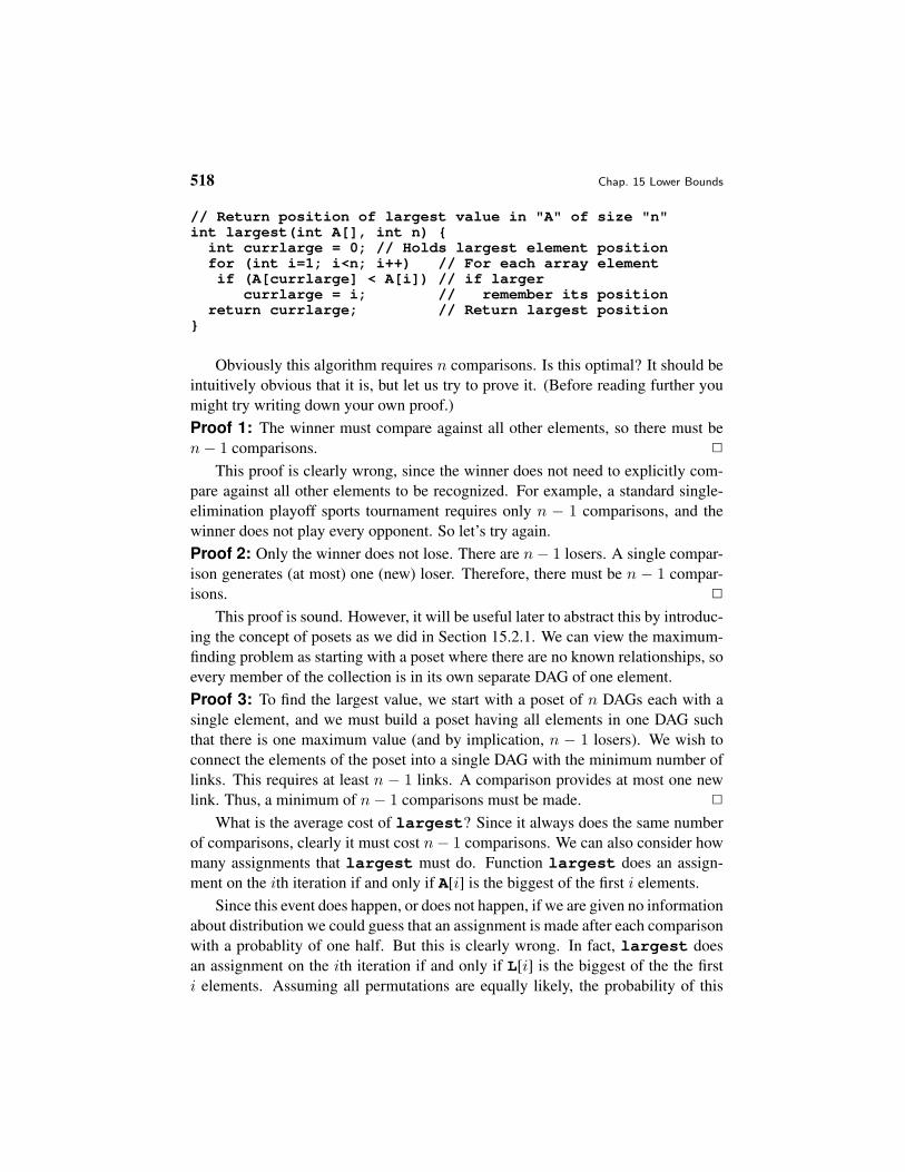
// Return position of largest value in "A" of size "n"int largest(int A[], int n)

int currlarge = 0; // Holds largest element positionfor (int i=1; i<n; i++) // For each array elementif (A[currlarge] < A[i]) // if larger

currlarge = i; // remember its positionreturn currlarge; // Return largest position

Obviously this algorithm requires n comparisons. Is this optimal? It should beintuitively obvious that it is, but let us try to prove it. (Before reading further youmight try writing down your own proof.)Proof 1: The winner must compare against all other elements, so there must ben− 1 comparisons. 2

This proof is clearly wrong, since the winner does not need to explicitly com-pare against all other elements to be recognized. For example, a standard single-elimination playoff sports tournament requires only n − 1 comparisons, and thewinner does not play every opponent. So let’s try again.Proof 2: Only the winner does not lose. There are n− 1 losers. A single compar-ison generates (at most) one (new) loser. Therefore, there must be n − 1 compar-isons. 2

This proof is sound. However, it will be useful later to abstract this by introduc-ing the concept of posets as we did in Section 15.2.1. We can view the maximum-finding problem as starting with a poset where there are no known relationships, soevery member of the collection is in its own separate DAG of one element.Proof 3: To find the largest value, we start with a poset of n DAGs each with asingle element, and we must build a poset having all elements in one DAG suchthat there is one maximum value (and by implication, n − 1 losers). We wish toconnect the elements of the poset into a single DAG with the minimum number oflinks. This requires at least n − 1 links. A comparison provides at most one newlink. Thus, a minimum of n− 1 comparisons must be made. 2

What is the average cost of largest? Since it always does the same numberof comparisons, clearly it must cost n− 1 comparisons. We can also consider howmany assignments that largest must do. Function largest does an assign-ment on the ith iteration if and only if A[i] is the biggest of the first i elements.

Since this event does happen, or does not happen, if we are given no informationabout distribution we could guess that an assignment is made after each comparisonwith a probablity of one half. But this is clearly wrong. In fact, largest doesan assignment on the ith iteration if and only if L[i] is the biggest of the the firsti elements. Assuming all permutations are equally likely, the probability of this

Sec. 15.4 Adversarial Lower Bounds Proofs 519

being true is 1/i. Thus, the average number of assignments done is

1 +n∑

i=2

1i

=n∑

i=1

1i.

This sum defines the nth harmonic number, written Hn.Since i ≤ 2dlog ie, we know that 1/i ≥ 1/2dlog ie. Thus, if n = 2k then

H2k = 1 +12

+13

+ ... +12k

≥ 1 +12

+14

+14

+18

+18

+18

+18

+... +12k

= 1 +12

+24

+48

+ ...2k−1

2k

= 1 +k

2.

Using similar logic, H2k ≤ k + 12k . Thus, Hn = Θ(log n). More exactly, Hn is

close to loge n.How “reliable” is this average? That is, how much will a given run of the

program deviate from the mean cost? According to Cebysev’s Inequality, an obser-vation will fall within two standard deviations of the mean at least 75% of the time.For Largest, the variance is

Hn −π2

6= loge n− π2

6

The standard deviation is thus about√

loge n. So, 75% of the observations arebetween loge n − 2

√loge n and loge n + 2

√loge n. Is this a narrow spread or a

wide spread? Compared to the mean value, this spread is pretty wide, meaning thatthe number of assignments varies widely from run to run of the program.

15.4 Adversarial Lower Bounds Proofs

We next consider the problem of finding the second largest in a collection of ob-jects. Let’s first think about what happens in a standard single-elimination tourna-ment. Even if we assume that the “best” team wins in every game, is the secondbest the one who loses in the finals? Not necessarily. We might expect that thesecond best must lose to best, but they might meet at any time.


Let us go through our standard “algorithm for finding algorithms” by firstproposing an algorithm, then a lower bound, and seeing if they match. Unlikeour analysis for most problems, this time we are going to count the exact numberof comparisons involved and attempt to minimize them. A simple algorithm forsolving the problem is to first find the maximum (in n− 1 comparisons), discard it,and then find the maximum of the remaining elements (in n− 2 comparisons) for atotal cost of 2n− 3 comparisions. Is this optimal? That seems doubtful, but let usnow proceed to attempting to prove a lower bound.Proof: Any element that loses to another that is not the maximum cannot be sec-ond. So, the only candidates for second place are those that lost to the maximum.Function largest might compare the maximum element to n − 1 others. Thus,we might need n− 2 additional comparisons to find the second largest. 2

This proof is wrong. It exhibits the necessity fallacy: “Our algorithm doessomething, therefore all algorithms solving the problem must do the same.”

This leaves us with our best lower bounds argument being that finding the sec-ond largest must cost at least as much as finding the largest, or n− 1. So let’s takeanother try at finding a better algorithm by adopting a strategy of divide and con-quer. What if we break the list into halves, and run largest on each half? We canthen compare the two winners (we have now used a total of n − 1 comparisons),and remove the winner from its half. Another call to largest on the winner’shalf yields its second best. A final comparison against the winner of the other halfgives us the true second place winner. The total cost is d3n/2e−2. Is this optimal?What if we break the list into four pieces? The best would be d5n/4e − 1. What ifwe break the list into eight pieces? Then the cost would be d9n/8e.

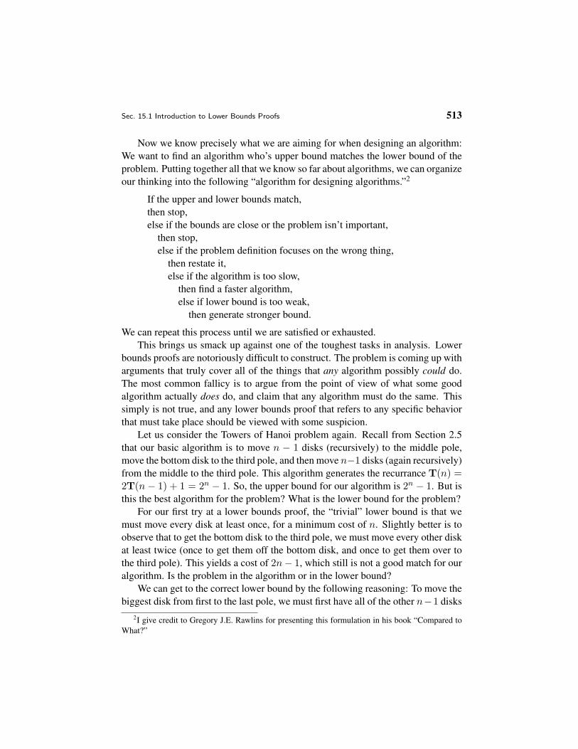
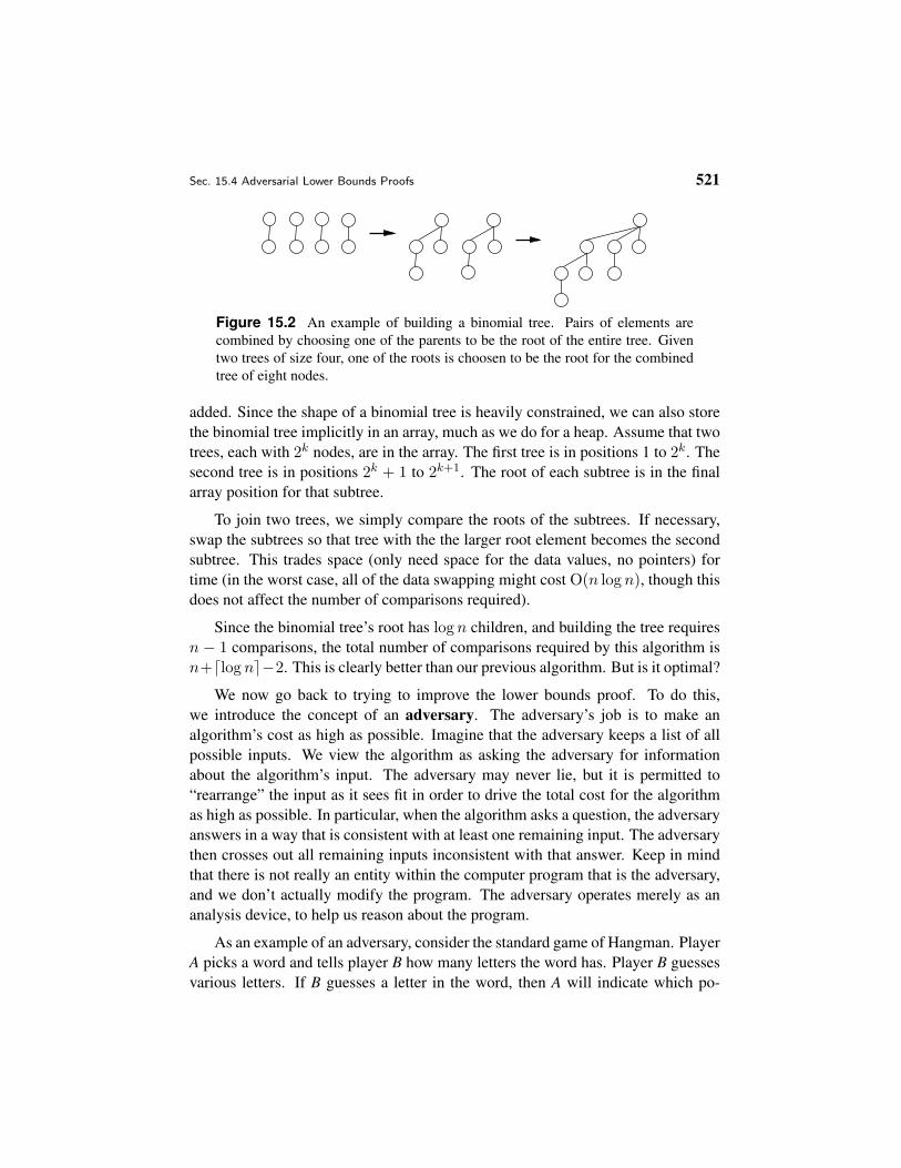
Pushing this idea to its extreme, the only candidates for second place are losersto the eventual winner, and our goal is to have as few of these as possible. Sowe need to keep track of the set of elements that have lost in direct comparisonto the (eventual) winnner. We also observe that we learn the most from a com-parison when both competitors are known to be larger than the same number ofother values. So we would like to arrange our comparisons to be against “equallystrong” competitors. We can do all of this with a binomial tree. A binomial tree ofheight m has 2m nodes. Either it is a single node (if m = 0), or else it is two heightm−1 binomial trees with one tree’s root becoming a child of the other. Figure 15.2illustrates how a binomial tree with eight nodes would be constructed.

The resulting algorithm is simple in principle: Build the binomial tree for all nelements, and then compare the dlog ne children of the root to find second place.We could store the binomial tree as an explicit tree structure, and easily build it intime linear on the number of comparisons as each comparison requires one link be

Sec. 15.4 Adversarial Lower Bounds Proofs 521

Figure 15.2 An example of building a binomial tree. Pairs of elements arecombined by choosing one of the parents to be the root of the entire tree. Giventwo trees of size four, one of the roots is choosen to be the root for the combinedtree of eight nodes.

added. Since the shape of a binomial tree is heavily constrained, we can also storethe binomial tree implicitly in an array, much as we do for a heap. Assume that twotrees, each with 2k nodes, are in the array. The first tree is in positions 1 to 2k. Thesecond tree is in positions 2k + 1 to 2k+1. The root of each subtree is in the finalarray position for that subtree.

To join two trees, we simply compare the roots of the subtrees. If necessary,swap the subtrees so that tree with the the larger root element becomes the secondsubtree. This trades space (only need space for the data values, no pointers) fortime (in the worst case, all of the data swapping might cost O(n log n), though thisdoes not affect the number of comparisons required).

Since the binomial tree’s root has log n children, and building the tree requiresn − 1 comparisons, the total number of comparisons required by this algorithm isn+dlog ne−2. This is clearly better than our previous algorithm. But is it optimal?

We now go back to trying to improve the lower bounds proof. To do this,we introduce the concept of an adversary. The adversary’s job is to make analgorithm’s cost as high as possible. Imagine that the adversary keeps a list of allpossible inputs. We view the algorithm as asking the adversary for informationabout the algorithm’s input. The adversary may never lie, but it is permitted to“rearrange” the input as it sees fit in order to drive the total cost for the algorithmas high as possible. In particular, when the algorithm asks a question, the adversaryanswers in a way that is consistent with at least one remaining input. The adversarythen crosses out all remaining inputs inconsistent with that answer. Keep in mindthat there is not really an entity within the computer program that is the adversary,and we don’t actually modify the program. The adversary operates merely as ananalysis device, to help us reason about the program.

As an example of an adversary, consider the standard game of Hangman. PlayerA picks a word and tells player B how many letters the word has. Player B guessesvarious letters. If B guesses a letter in the word, then A will indicate which po-


sition(s) in the word have the letter. Player B is permitted to make only so manyguesses of letters not in the word before losing.

In the Hangman game example, the adversary is imagined to hold a dictionaryof words of some selected length. Each time the player guesses a letter, the ad-versary consults the dictionary and decides if more words will be eliminated byaccepting the letter (and indicating which positions it holds) or saying that its notin the word. The adversary can make any decision it chooses, so long as at leastone word in the dictionary is consistent with all of the decisions. In this way, theadversary can hope to make the player guess as many letters as possible.

Before explaining how the adversary plays a role in our lower bounds proof,first observe that at least n− 1 values must lose at least once. This requires at leastn − 1 compares. In addition, at least k − 1 values must lose to the second largestvalue. I.e., k direct losers to the winner must be compared. There must be at leastn + k − 2 comparisons. The question is: How low can we make k?

Call the strength of element A[i] the number of elements that A[i] is (known tobe) bigger than. If A[i] has strength a, and A[j] has strength b, then the winner hasstrength a + b + 1. What strategy by the adversary would cause the algorithm tolearn the least from any given comparison? It should minimize the rate at which anyelement improves it strength. It can do this by making the element with the greaterstrength win at every comparison. This is a “fair” use of an adversary in that itrepresents the results of providing a worst-case input for that given algorithm.

To minimize the effects of worst-case behavior, the algorithm’s best strategy isto maximize the minimum improvement in strength by balancing the strengths ofany two competitors. From the algorithm’s point of view, the best outcome is thatan element doubles in strength. This happens whenever a = b, where a and b arethe strengths of the two elements being compared. All strengths begin at zero, sothe winner must make at least k comparisons since 2k−1 < n ≤ 2k. Thus, theremust be at least n + dlog ne − 2 comparisons. Therefore, our algorithm is optimal.

15.5 State Space Lower Bound

We now consider the problem of finding both the minimum and the maximum froman (unsorted) list of values. This might be useful if we want to know the range ofa collection of values to be plotted, for the purpose of drawing the plot’s scales.Of course we could find them independently in 2n − 2 comparisons. A slightmodification is to find the maximum in n − 1 comparisons, remove it from thelist, and then find the minimum in n − 2 further comparisons for a total of 2n − 3comparisons. Can we do better than this?

Sec. 15.5 State Space Lower Bound 523

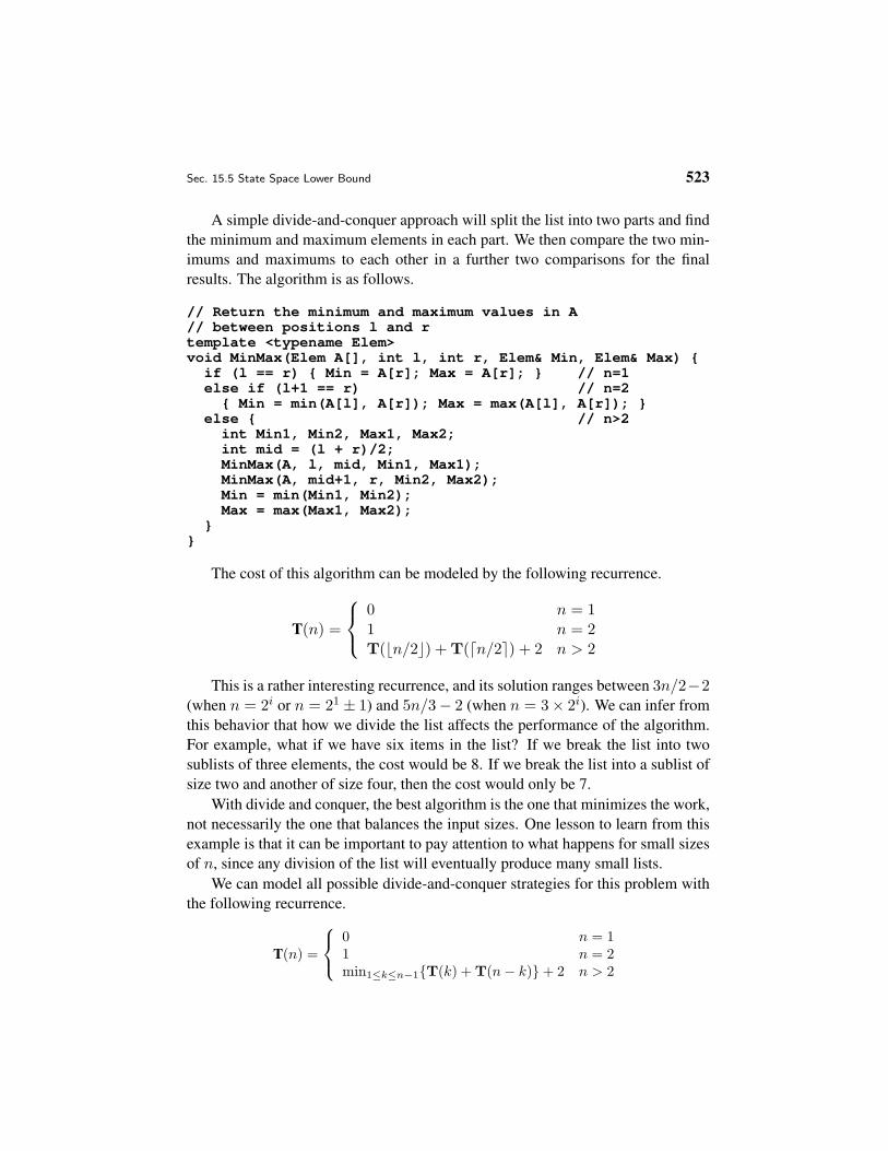
A simple divide-and-conquer approach will split the list into two parts and findthe minimum and maximum elements in each part. We then compare the two min-imums and maximums to each other in a further two comparisons for the finalresults. The algorithm is as follows.

// Return the minimum and maximum values in A// between positions l and rtemplate <typename Elem>void MinMax(Elem A[], int l, int r, Elem& Min, Elem& Max)

if (l == r) Min = A[r]; Max = A[r]; // n=1else if (l+1 == r) // n=2

Min = min(A[l], A[r]); Max = max(A[l], A[r]); else // n>2

int Min1, Min2, Max1, Max2;int mid = (l + r)/2;MinMax(A, l, mid, Min1, Max1);MinMax(A, mid+1, r, Min2, Max2);Min = min(Min1, Min2);Max = max(Max1, Max2);

The cost of this algorithm can be modeled by the following recurrence.

T(n) =

0 n = 11 n = 2T(bn/2c) + T(dn/2e) + 2 n > 2

This is a rather interesting recurrence, and its solution ranges between 3n/2−2(when n = 2i or n = 21 ± 1) and 5n/3− 2 (when n = 3× 2i). We can infer fromthis behavior that how we divide the list affects the performance of the algorithm.For example, what if we have six items in the list? If we break the list into twosublists of three elements, the cost would be 8. If we break the list into a sublist ofsize two and another of size four, then the cost would only be 7.

With divide and conquer, the best algorithm is the one that minimizes the work,not necessarily the one that balances the input sizes. One lesson to learn from thisexample is that it can be important to pay attention to what happens for small sizesof n, since any division of the list will eventually produce many small lists.

We can model all possible divide-and-conquer strategies for this problem withthe following recurrence.

T(n) =

0 n = 11 n = 2min1≤k≤n−1T(k) + T(n− k)+ 2 n > 2


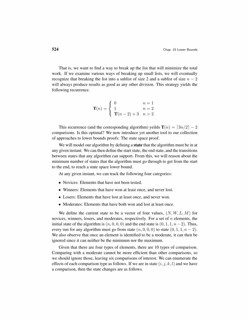
That is, we want to find a way to break up the list that will minimize the totalwork. If we examine various ways of breaking up small lists, we will eventuallyrecognize that breaking the list into a sublist of size 2 and a sublist of size n − 2will always produce results as good as any other division. This strategy yields thefollowing recurrence.

T(n) =

0 n = 11 n = 2T(n− 2) + 3 n > 2

This recurrence (and the corresponding algorithm) yeilds T(n) = d3n/2e − 2comparisons. Is this optimal? We now introduce yet another tool to our collectionof approaches to lower bounds proofs: The state space proof.

We will model our algorithm by defining a state that the algorithm must be in atany given instant. We can then define the start state, the end state, and the transitionsbetween states that any algorithm can support. From this, we will reason about theminimum number of states that the algorithm must go through to get from the startto the end, to reach a state space lower bound.

At any given instant, we can track the following four categories:

• Novices: Elements that have not been tested.

• Winners: Elements that have won at least once, and never lost.

• Losers: Elements that have lost at least once, and never won.

• Moderates: Elements that have both won and lost at least once.

We define the current state to be a vector of four values, (N,W,L,M) fornovices, winners, losers, and moderates, respectively. For a set of n elements, theinitial state of the algorithm is (n, 0, 0, 0) and the end state is (0, 1, 1, n− 2). Thus,every run for any algorithm must go from state (n, 0, 0, 0) to state (0, 1, 1, n − 2).We also observe that once an element is identified to be a moderate, it can then beignored since it can neither be the minimum nor the maximum.

Given that there are four types of elements, there are 10 types of comparison.Comparing with a moderate cannot be more efficient than other comparisons, sowe should ignore those, leaving six comparisons of interest. We can enumerate theeffects of each comparison type as follows. If we are in state (i, j, k, l) and we havea comparison, then the state changes are as follows.

Sec. 15.6 Finding the ith Best Element 525

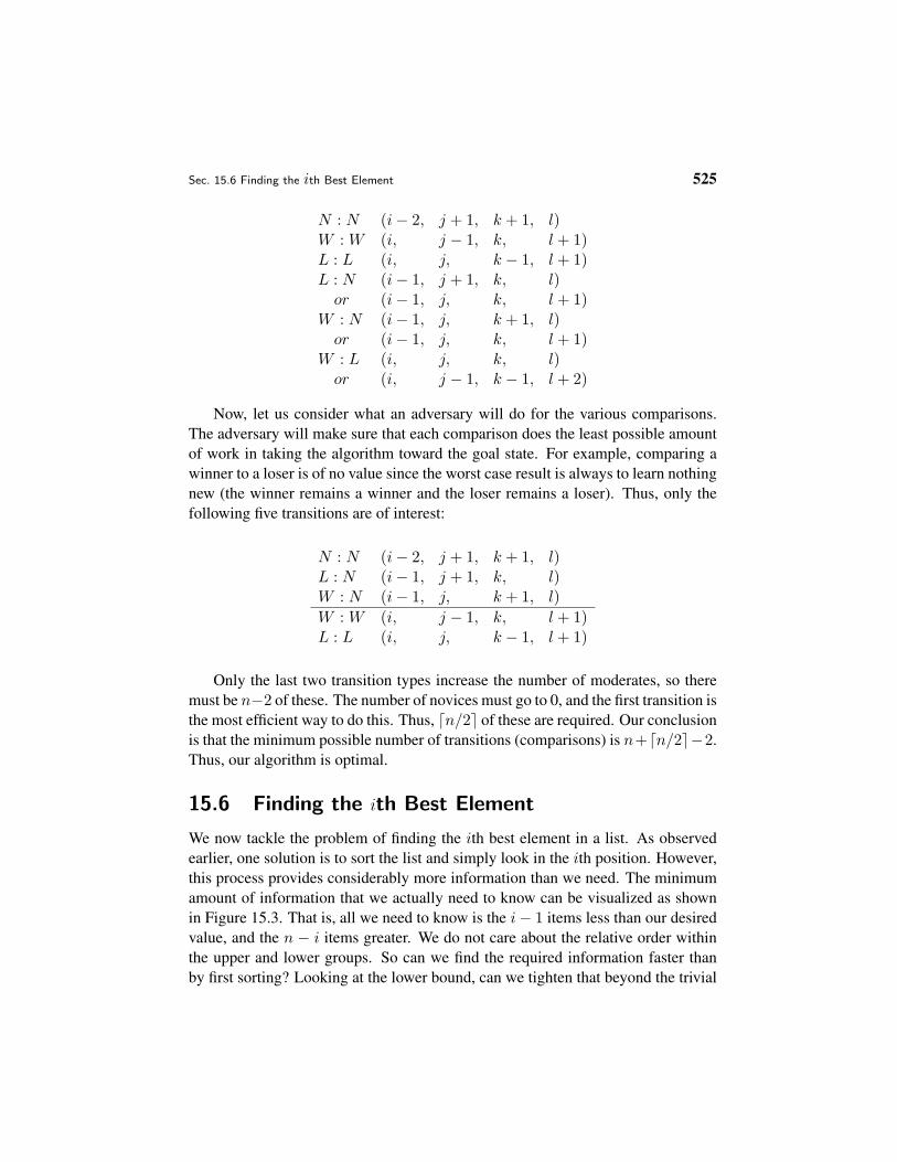
N : N (i− 2, j + 1, k + 1, l)W : W (i, j − 1, k, l + 1)L : L (i, j, k − 1, l + 1)L : N (i− 1, j + 1, k, l)

or (i− 1, j, k, l + 1)W : N (i− 1, j, k + 1, l)

or (i− 1, j, k, l + 1)W : L (i, j, k, l)

or (i, j − 1, k − 1, l + 2)

Now, let us consider what an adversary will do for the various comparisons.The adversary will make sure that each comparison does the least possible amountof work in taking the algorithm toward the goal state. For example, comparing awinner to a loser is of no value since the worst case result is always to learn nothingnew (the winner remains a winner and the loser remains a loser). Thus, only thefollowing five transitions are of interest:

N : N (i− 2, j + 1, k + 1, l)L : N (i− 1, j + 1, k, l)W : N (i− 1, j, k + 1, l)W : W (i, j − 1, k, l + 1)L : L (i, j, k − 1, l + 1)

Only the last two transition types increase the number of moderates, so theremust be n−2 of these. The number of novices must go to 0, and the first transition isthe most efficient way to do this. Thus, dn/2e of these are required. Our conclusionis that the minimum possible number of transitions (comparisons) is n+dn/2e−2.Thus, our algorithm is optimal.

15.6 Finding the ith Best Element

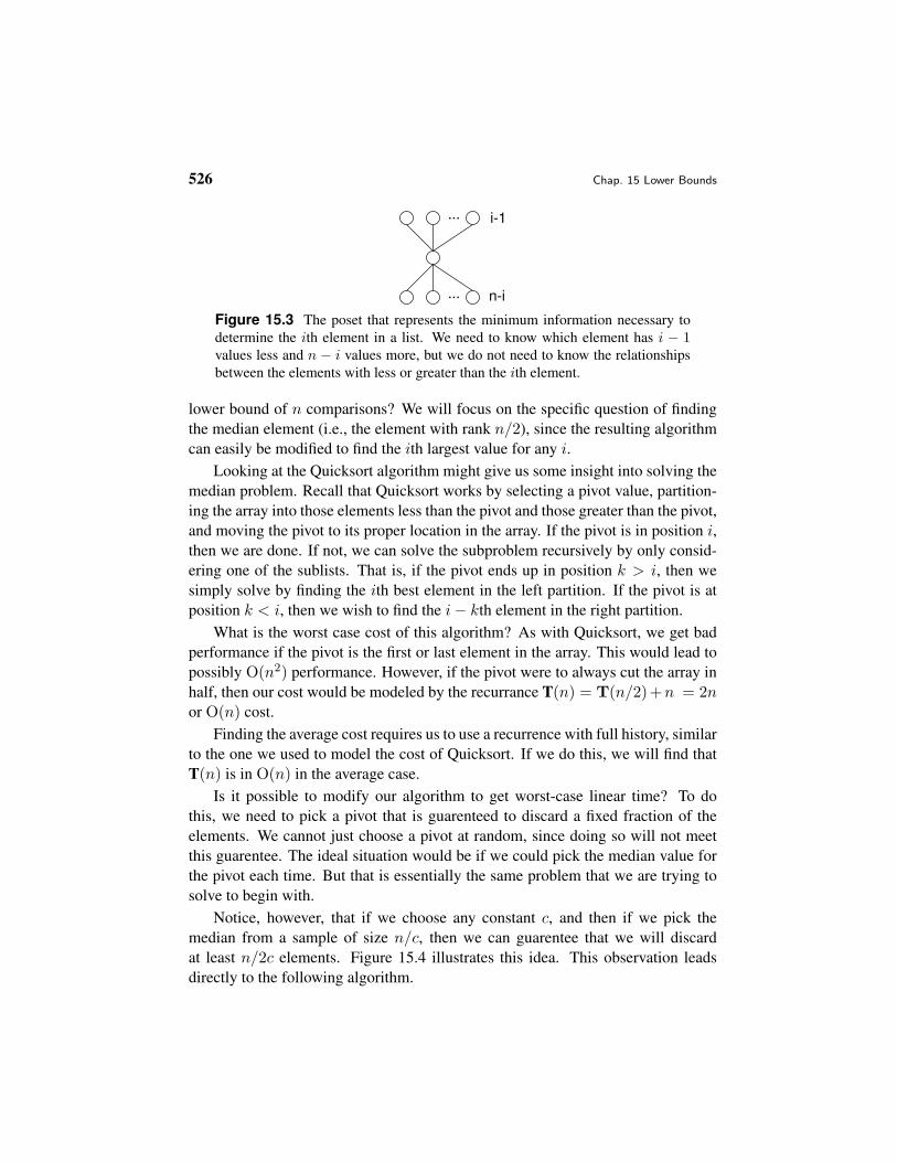
We now tackle the problem of finding the ith best element in a list. As observedearlier, one solution is to sort the list and simply look in the ith position. However,this process provides considerably more information than we need. The minimumamount of information that we actually need to know can be visualized as shownin Figure 15.3. That is, all we need to know is the i− 1 items less than our desiredvalue, and the n − i items greater. We do not care about the relative order withinthe upper and lower groups. So can we find the required information faster thanby first sorting? Looking at the lower bound, can we tighten that beyond the trivial


...

... i-1

n-i

Figure 15.3 The poset that represents the minimum information necessary todetermine the ith element in a list. We need to know which element has i − 1values less and n − i values more, but we do not need to know the relationshipsbetween the elements with less or greater than the ith element.

lower bound of n comparisons? We will focus on the specific question of findingthe median element (i.e., the element with rank n/2), since the resulting algorithmcan easily be modified to find the ith largest value for any i.

Looking at the Quicksort algorithm might give us some insight into solving themedian problem. Recall that Quicksort works by selecting a pivot value, partition-ing the array into those elements less than the pivot and those greater than the pivot,and moving the pivot to its proper location in the array. If the pivot is in position i,then we are done. If not, we can solve the subproblem recursively by only consid-ering one of the sublists. That is, if the pivot ends up in position k > i, then wesimply solve by finding the ith best element in the left partition. If the pivot is atposition k < i, then we wish to find the i− kth element in the right partition.

What is the worst case cost of this algorithm? As with Quicksort, we get badperformance if the pivot is the first or last element in the array. This would lead topossibly O(n2) performance. However, if the pivot were to always cut the array inhalf, then our cost would be modeled by the recurrance T(n) = T(n/2)+n = 2nor O(n) cost.

Finding the average cost requires us to use a recurrence with full history, similarto the one we used to model the cost of Quicksort. If we do this, we will find thatT(n) is in O(n) in the average case.

Is it possible to modify our algorithm to get worst-case linear time? To dothis, we need to pick a pivot that is guarenteed to discard a fixed fraction of theelements. We cannot just choose a pivot at random, since doing so will not meetthis guarentee. The ideal situation would be if we could pick the median value forthe pivot each time. But that is essentially the same problem that we are trying tosolve to begin with.

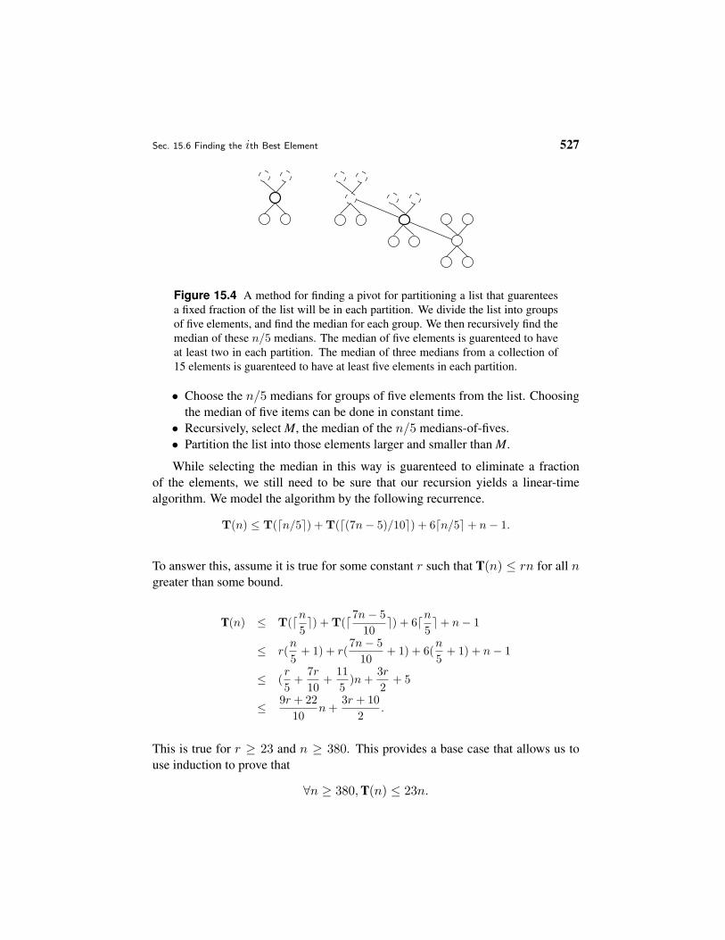
Notice, however, that if we choose any constant c, and then if we pick themedian from a sample of size n/c, then we can guarentee that we will discardat least n/2c elements. Figure 15.4 illustrates this idea. This observation leadsdirectly to the following algorithm.

Sec. 15.6 Finding the ith Best Element 527

Figure 15.4 A method for finding a pivot for partitioning a list that guarenteesa fixed fraction of the list will be in each partition. We divide the list into groupsof five elements, and find the median for each group. We then recursively find themedian of these n/5 medians. The median of five elements is guarenteed to haveat least two in each partition. The median of three medians from a collection of15 elements is guarenteed to have at least five elements in each partition.

• Choose the n/5 medians for groups of five elements from the list. Choosingthe median of five items can be done in constant time.

• Recursively, select M, the median of the n/5 medians-of-fives.• Partition the list into those elements larger and smaller than M.

While selecting the median in this way is guarenteed to eliminate a fractionof the elements, we still need to be sure that our recursion yields a linear-timealgorithm. We model the algorithm by the following recurrence.

T(n) ≤ T(dn/5e) + T(d(7n− 5)/10e) + 6dn/5e+ n− 1.

To answer this, assume it is true for some constant r such that T(n) ≤ rn for all ngreater than some bound.

T(n) ≤ T(dn5e) + T(d7n− 5

10e) + 6dn

5e+ n− 1

≤ r(n

5+ 1) + r(

7n− 510

+ 1) + 6(n

5+ 1) + n− 1

≤ (r

5+

7r

10+

115

)n +3r

2+ 5

≤ 9r + 2210

n +3r + 10

2.

This is true for r ≥ 23 and n ≥ 380. This provides a base case that allows us touse induction to prove that

∀n ≥ 380, T(n) ≤ 23n.


In reality, this algorithm is not practical. It is more efficient on average to relyon chance to select the pivot, perhaps by picking it at random or picking the middlevalue out of the current subarray.

15.7 Optimal Sorting

We conclude this section with an effort to find the sorting algorithm with the ab-solute fewest possible comparisons. It might well be that the result will not bepractical for a general-purpose sorting algorithm. But recall our analogy earlier tosports tournaments. In sports, a “comparison” between two teams or individualsmeans doing a competition between the two. This is fairly expensive (at least com-pared to some minor book keeping in a computer), and it might be worth trading afair amount of book keeping to cut down on the number of games that need to beplayed. What if we want to figure out how to hold a tournament that will give usthe exact ordering for all teams in the fewest number of total games? Of course,we are assuming that the results of each game will be “accurate” in that we assumenot only that the outcome of A playing B would always be the same (at least overthe time period of the tournament), but that transitivity in the results also holds. Inpractice these are unrealistic assumptions, but such assumptions are implicitly partof many tournament organizations. Like most tournament organizers, we can sim-ply accept these assumptions and come up with an algorithm for playing the gamesthat gives us some rank ordering based on the results we obtain.

Recall Insertion Sort, where we put element i into a sorted sublist of the first i−1 elements. What if we modify the standard Insertion Sort algorithm to use binarysearch to locate where the ith element goes in the sorted sublist? This algorithmis called binary insert sort. As a general-purpose sorting algorithm, this is notpractical because we then have to (on average) move about i/2 elements to makeroom for the newly inserted element in the sorted sublist. But if we count onlycomparisons, binary insert sort is pretty good. And we can use some ideas frombinary insert sort to get closer to an algorithm that uses the absolute minimumnumber of comparisons needed to sort.

Consider what happens when we run binary insert sort on five elements. Howmany comparisons do we need to do? We can insert the second element with onecomparison, the third with two comparisons, and the fourth with 2 comparisons.When we insert the fifth element into the sorted list of four elements, we need to dothree comparisons in the worst case. Notice exactly what happens when we attemptto do this insertion. We compare the fifth element against the second. If the fifth isbigger, we have to compare it against the third, and if its bigger we have to compareit against the fourth. In general, when is binary search most efficient? When we

Sec. 15.7 Optimal Sorting 529

AB

orA

A

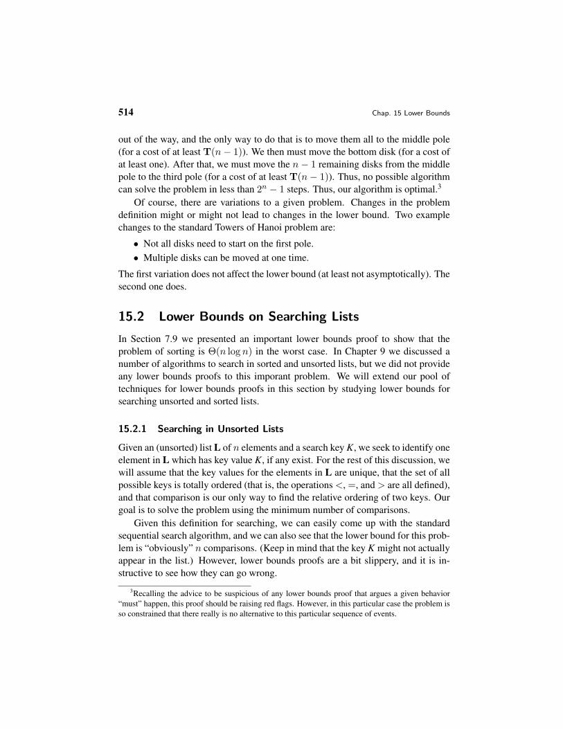
Figure 15.5 Organizing comparisons for sorting five elements. First we ordertwo pairs of elements, and then compare the two winners to form a binomial treeof four elements. The original loser to the root is labeled A, and the remainingthree elements form a sorted chain. We then insert element B into the sortedchain. Finally, we put A into resulting sorted chain of four elements to yield afinal sorted list.

have 2i − 1 elements in the list. It is least efficient when we have 2i elements inthe list. So, we can do a bit better if we arrange our insertions to avoid inserting anelement into a list of size 2i if possible.

Figure 15.5 illustrates a different organization for the comparisons that wemight do. First we compare the first and second element, and the third and fourthelements. The two winners are then compared, yielding a binomial tree. We canview this as a (sorted) chain of three elements, with element A hanging off from theroot. If we then insert element B into the sorted chain of three elements, we willend up with one of the two posets shown on the right side of Figure 15.5, at a cost of2 comparisons. We can then merge A into the chain, for a cost of two comparisons(since we already know that it is smaller then either one or two elements, we areactually merging it into a list of two or three elements). Thus, the total number ofcomparisons needed to sort the five elements is at most seven instead of eight.

If we have ten elements to sort, we can first make five pairs of elements (usingfive compares) and then sort the five winners using the algorithm just described(using seven more compares). Now all we need to do is to deal with the originallosers. We can generalize this process for any number of elements as:

• Pair up all the nodes with bn2 c comparisons.

• Recursively sort the winners.• Fold in the losers.

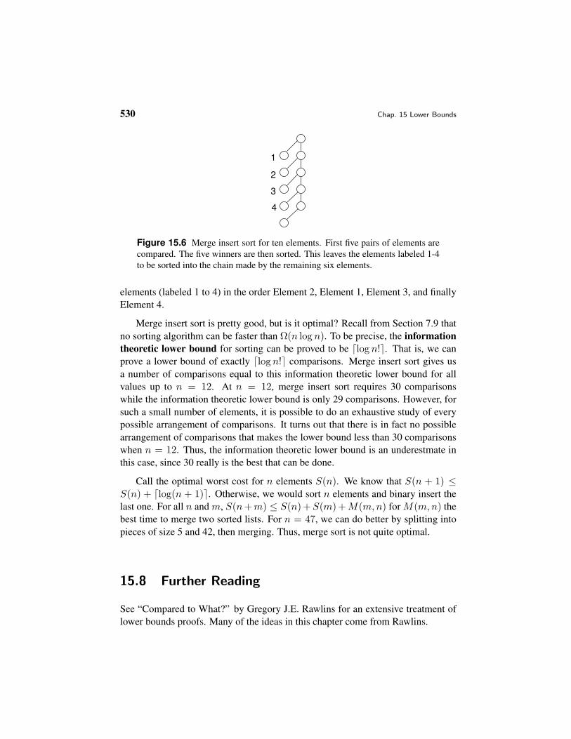
We will use binary insert to place the losers. However, we are free to choosethe best ordering for inserting, keeping in mind the fact that binary search is bestfor 2i − 1 items. So we pick the order of inserts to optimize the binary searches.This sort is called merge insert sort, and also known as the Ford and Johnson sort.For ten elements, given the poset shown in Figure 15.6 we fold in the last four


1

2

4

3

Figure 15.6 Merge insert sort for ten elements. First five pairs of elements arecompared. The five winners are then sorted. This leaves the elements labeled 1-4to be sorted into the chain made by the remaining six elements.

elements (labeled 1 to 4) in the order Element 2, Element 1, Element 3, and finallyElement 4.

Merge insert sort is pretty good, but is it optimal? Recall from Section 7.9 thatno sorting algorithm can be faster than Ω(n log n). To be precise, the informationtheoretic lower bound for sorting can be proved to be dlog n!e. That is, we canprove a lower bound of exactly dlog n!e comparisons. Merge insert sort gives usa number of comparisons equal to this information theoretic lower bound for allvalues up to n = 12. At n = 12, merge insert sort requires 30 comparisonswhile the information theoretic lower bound is only 29 comparisons. However, forsuch a small number of elements, it is possible to do an exhaustive study of everypossible arrangement of comparisons. It turns out that there is in fact no possiblearrangement of comparisons that makes the lower bound less than 30 comparisonswhen n = 12. Thus, the information theoretic lower bound is an underestmate inthis case, since 30 really is the best that can be done.

Call the optimal worst cost for n elements S(n). We know that S(n + 1) ≤S(n) + dlog(n + 1)e. Otherwise, we would sort n elements and binary insert thelast one. For all n and m, S(n + m) ≤ S(n) + S(m) + M(m,n) for M(m,n) thebest time to merge two sorted lists. For n = 47, we can do better by splitting intopieces of size 5 and 42, then merging. Thus, merge sort is not quite optimal.

15.8 Further Reading

See “Compared to What?” by Gregory J.E. Rawlins for an extensive treatment oflower bounds proofs. Many of the ideas in this chapter come from Rawlins.

Sec. 15.9 Exercises 531

15.9 Exercises

15.1 Consider the so-called “algorithm for algorithms” in Section 15.1. Is thisreally an algorithm? Review the definition of an algorithm from Section 1.4.Which parts of the definition apply, and which do not? Is the “algorithm foralgorithms” a heuristic for finding a good algorithm? Why or why not?

15.2 Single-elimination tournaments are notorious for their scheduling difficul-ties. Imagine that you are organizing a tournament for n basketball teams(you may assume that n = 2i for some integer i). We will further simplifythings by assuming that each game takes less than an hour, and that each teamcan be scheduled for a game every hour if necessary. (Note that everythingsaid here about basketball courts is also true about processors in a parallelalgorithm to solve the maximum-finding problem).

(a) How many basketball courts do we need to insure that every team canplay whenever we want to minimize the total tournament time?

(b) How long will the tournament be in this case?(c) What is the total number of “court-hours” available? How many total

hours are courts being used? How many hours are courts unused?(d) Modify the algorithm in such a way as to reduce the total number of

courts needed, by perhaps not letting every team play whenever possi-ble. This will increase the total hours of the tournament, but try to keepthe increase as low as possible. For your new algorithm, how long is thetournament, how many courts are needed, how many total court-hoursare available, how many court-hours are used, and how many unused?

15.3 Explain why the cost of splitting a list of six into two lists of three to find theminimum and maximum elements requires eight comparisons, while split-ting the list into a list of two and a list of four costs only seven comparisons.

15.4 Write out a table showing the number of comparisons required to find theminimum and maximum for all divisions for all values of n ≤ 13.

15.5 (a) Write an equation to describe the average cost for finding the median.(b) Solve your equation from part (a).

15.6 (a) Write an equation to describe the average cost for finding the ith-smallestvalue in an array. This will be a function of both n and i, T(n, i).

(b) Solve your equation from part (a).15.7 Imagine that you are organizing a basketball tournament for 10 teams. You

know that the merge insert sort will give you a full ranking of the 10 teamswith the minimum number of games played. Assume that each game can beplayed in less than an hour, and that any team can play as many games in


a row as necessary. Show a schedule for this tournament that also attemptsto minimize the number of total hours for the tournament and the number ofcourts used. If you have to make a tradeoff between the two, then attempt tominimize the total number of hours that basketball courts are idle.

15.8 Write the complete algorithm for the merge insert sort sketched out in Sec-tion 15.7.

15.9 Here is a suggestion for might be a truly optimal sorting algorithm. Pick thebest set of comparisons for input lists of size 2. Then pick the best set ofcomparisons for size 3, 4, 5, and so on. Combine them together into oneprogram with a big case statement. Is this an algorithm?

15.10 Projects

15.1 Implement the median-finding algorithm of Section 15.6. Then, modify thisalgorithm to allow finding the ith element for any value i < n.

15 lower bounds - courses

Documents