This article was downloaded by:[Finel, B.]On: 1 June 2008Access Details: [subscription number 793293252]Publisher: Taylor & FrancisInforma Ltd Registered in England and Wales Registered Number: 1072954Registered office: Mortimer House, 37-41 Mortimer Street, London W1T 3JH, UK

International Journal of ComputerIntegrated ManufacturingPublication details, including instructions for authors and subscription information:http://www.informaworld.com/smpp/title~content=t713804665

A random search and backtracking procedure fortransfer line balancingB. Finel a; A. Dolgui b; F. Vernadat aa LGIPM, ENIM/University of Metz, Franceb Ecole des Mines de Saint Etienne, France

First Published: June 2008

To cite this Article: Finel, B., Dolgui, A. and Vernadat, F. (2008) 'A random searchand backtracking procedure for transfer line balancing', International Journal ofComputer Integrated Manufacturing, 21:4, 376 — 387

To link to this article: DOI: 10.1080/09511920701574172URL: http://dx.doi.org/10.1080/09511920701574172

PLEASE SCROLL DOWN FOR ARTICLE

Full terms and conditions of use: http://www.informaworld.com/terms-and-conditions-of-access.pdf

This article maybe used for research, teaching and private study purposes. Any substantial or systematic reproduction,re-distribution, re-selling, loan or sub-licensing, systematic supply or distribution in any form to anyone is expresslyforbidden.

The publisher does not give any warranty express or implied or make any representation that the contents will becomplete or accurate or up to date. The accuracy of any instructions, formulae and drug doses should beindependently verified with primary sources. The publisher shall not be liable for any loss, actions, claims, proceedings,demand or costs or damages whatsoever or howsoever caused arising directly or indirectly in connection with orarising out of the use of this material.

Dow

nloa

ded

By:

[Fin

el, B

.] A

t: 22

:25

1 Ju

ne 2

008

A random search and backtracking procedure fortransfer line balancing

B. FINEL*{, A. DOLGUI{ and F. VERNADAT{

{LGIPM, ENIM/University of Metz, France{Ecole des Mines de Saint Etienne, France

The optimal logical layout design for a type of machining transfer lines is addressed. Such

transfer lines are made of many machine-tools (workstations) located in sequence. On

each workstation there are several spindle-heads. A spindle-head does not execute a single

operation but a block of machining operations; all operations of a block are executed

simultaneously (in parallel). Spindle-heads of the same workstation are activated

sequentially in a fixed order. The transfer line design problem considered in the paper

consists of finding the best partition in blocks and workstations of the set of all operations

to be executed on the line. The objective is to minimize the number of spindle-heads and

workstations (i.e. transfer line investment cost). An optimal decision must satisfy a desired

productivity rate (cycle time) as well as precedence and compatibility constraints for

machining operations. A heuristic algorithm is proposed: it is based on the COMSOAL

technique and a backtracking approach. Results from computer testing are reported.

Keywords: Transfer lines; Line balancing; Optimization; Heuristic algorithms

1. Introduction

When mechanical industries want to produce a large

quantity of homogeneous products, they often use dedicated

transfer lines (Groover 1987, Hitomi 1996, Dashchenko

2003). To design such types of machining lines it is necessary

to follow three interconnected steps (Dolgui et al. 2006a):

1. the selection of the necessary operations to machine

a part;

2. the logical layout design, i.e. the logical synthesis of

the manufacturing process, which consists of group-

ing the operations into blocks (spindle-heads) and

the blocks into stations;

3. the physical layout and equipment (tools, spindle-

heads, etc.) design depending on the logical layout

decided.

This paper concerns the logical layout design stage

assuming that all the required operations to manufacture

a product as well as constraints of the physical layout are

known.

Pieces of equipment involved in such lines represent a

significant investment cost. Thus, finding a good (and if

possible the best) logical layout design decision that

minimizes their number is a crucial problem (Martin and

D’Acunto 2003). The aim of our study is to minimize the

number of workstations and spindle-heads at the prelimin-

ary design stage of the line.

To minimize the number of workstations and spindle-

heads (line cost) as well as the occupied floor area for the

considered line, the operations are grouped into blocks. All

operations of the same block are executed simultaneously

by one spindle-head (a spindle-head has many tools and

executes all the operations simultaneously). Thus, the

processing time of each block is equal to the longest

processing time for all operations of this block. All blocks

(spindle-heads) of the same station are executed sequen-

tially in a given order. The assignment of blocks to a station

defines at the same time the order of their activation on this

*Corresponding author. Email: finel@enim.fr

International Journal of Computer Integrated Manufacturing, Vol. 21, No. 4, June 2008, 376 – 387

International Journal of Computer Integrated ManufacturingISSN 0951-192X print/ISSN 1362-3052 online ª 2008 Taylor & Francis

http://www.tandf.co.uk/journalsDOI: 10.1080/09511920701574172

Dow

nloa

ded

By:

[Fin

el, B

.] A

t: 22

:25

1 Ju

ne 2

008

station. Therefore, the station processing time is equal to

the sum of block times (for all blocks assigned to this

station). All the stations are linearly ordered; there are no

buffers between stations. The bottleneck station defines the

transfer line cycle time. A line of this type is presented in

figure 1 (available online at www.pci.fr).

In this paper, the objective function is defined as follows

Minimize C ¼ mC1 þQ C2; ð1Þ

where

m is the number of stations (machine-tools),

Q is the total number of blocks (spindle-heads),

C1 and C2 are the weighted coefficients (can be interpreted

as relative unit costs) for stations and spindle-heads,

respectively.

The problem considered extends the well-known simple

assembly line balancing problem (SALBP). Some surveys

on techniques used to solve SALBP can be found in

(Baybars 1986, Boctor 1995, Erel and Sarin 1998, Ghosh

and Gagnon 1989, Scholl and Klein 1998, Rekiek et al.

2002). Talbot et al. (1986) present a comparison of heuristic

techniques including decisions rules with backtrack and

probabilistic search.

The SALBP method cannot be directly used for the

considered problem because of the grouping of the opera-

tions in blocks where all the operations of the same block

are executed simultaneously. Therefore, in our previous

publications, we suggested some dedicated methods.

Two exact optimization methods based on mixed

integer programming (MIP) and graph approaches,

respectively, were initially suggested in Dolgui et al.

(2000). An improved version of MIP model with some

pre-processing rules and cuts is presented by Dolgui et al.

(2006a). A more recent version of the graph approach is

given by Dolgui et al. (2006c). These exact optimization

methods can be used only for small and medium-sized

problems (*60 operations). For large-scale problems,

some simple heuristic approaches, based on the COM-

SOAL (Arcus 1966) techniques were developed by Dolgui

et al. (2005). Another heuristic approach based on

decomposition of the MIP model is suggested by Dolgui

et al. (2006b).

The COMSOAL based heuristics demonstrated good

performances for this problem. Therefore, it is interesting

to continue studying this type of heuristics. In this paper,

one of COMSOAL based heuristics is improved using a

new backtracking and learning procedure.

The paper is organized as follows. Section 2 introduces

some notations that define the problem. In section 3 a

known heuristic algorithm named RAP is explained.

Section 4 introduces a backtracking and learning procedure

to improve this heuristic algorithm. In section 5, numerical

examples, tests and comparisons are given. Conclusion

remarks are reported in section 6.

2. Problem statement

2.1. Notations

The purpose of the line balancing problem addressed herein

is to assign the operations to stations (machines) and to

blocks (spindle-heads) in such a way that:

(a) the objective function (1) is optimized;

(b) the specified line cycle time is not exceeded (i.e. the

obtained line cycle time is not greater than the

specified one);

(c) All the constraints for machining operations are

satisfied.

The following precedence and compatibility constraints are

taken into account.

(1) A partial order relation on the set of all operations

to be machined. This defines a set of possible

operations sequences (precedence constraints). In

this problem, taking into account the specificity of

the machining environment, ‘an operation i pre-

cedes an operation j’ means that the operation i can

be executed before the operation j or at the same

time as j (in the same block), but the operation

j cannot be executed before the operation i.

Figure 1. A transfer line with multiple spindle-heads.

(PCI/ SCEMM, Saint Etienne, France).

A random search and backtracking procedure for transfer line balancing 377

Dow

nloa

ded

By:

[Fin

el, B

.] A

t: 22

:25

1 Ju

ne 2

008

(2) The necessity to perform some groups of operations

on the same station (e.g. because of a required

machining tolerance);

(3) The impossibility to perform some groups of

operations within one block (e.g. due to spindle-

head design or because of manufacturing incompat-

ibility of operations);

(4) The impossibility to perform some groups of

operations on the same station (e.g. owing to

station design or because of manufacturing incom-

patibility of operations).

The following notations will be used throughout this

paper:

N given set of operations to be machined;

T0 desired transfer line cycle time;

m0 maximal authorized number of stations;

n0 maximal authorized number of blocks in one

station;

tj processing time of the operation j2N;

Pred(j) set of direct predecessors of the operation

j2N;

q0¼m0n0 maximal ID of blocks at the line;

k station number, k¼ 1, 2, . . ., m;

nk number of blocks at the station k;

Bq set of operations of the block q, i.e. Bq¼Nkl,

for q¼ (k7 1) n0þ l;

C(k) ‘cost’ of station k with all its blocks, i.e.

C(k)¼C1þC2nk;

Tk the slack time of station k;

S(k) set of the blocks (their numbers) which will

be executed by the station k,

S(k)¼ {(k7 1)n0þ 1, . . . k n0};

ES set of operation sets representing the exclu-

sion (i.e. impossibility) constraints for sta-

tions. Operations of the same set of the

collection cannot be assigned to the same

station all together;

EB set of operation sets representing the exclu-

sion (i.e. impossibility) constraints for

blocks. Operations of the same set of a

collection cannot be assigned to the same

block all together;

ES set of operation sets representing the inclu-

sion (i.e. necessity) constraints for the

stations. All operations of the same set of

the collection must be assigned to the same

station.

2.2. MIP formulation

To better explain the optimization problem considered, a

MIP formulation is presented in this section (for more

details see Dolgui et al. (2000, 2006a)). This model uses the

following binary variables:

Xiq ¼1; if the operation i is assigned to the block q;0; otherwise;

�

and the real variables:

Fq� 0, to determine block time, and Yq� 0 (Zk� 0), to

count the number of blocks (stations).

Minimize C1

Xm0

k¼1Zk þ C2

Xq0q¼1

Yq; ð2Þ

Subject to:

Xq0q¼1

Xjq ¼ 1; ð3Þ

Xi2PredðjÞ

Xq0�q

Xiq0 � Xjq Pred ðjÞj j; ð4Þ

Xj2e

Xjq � jej � 1; e 2 EB; ð5Þ

Xj2e

Xq2SðkÞ

Xjq � jej � 1; e 2 ES; ð6Þ

Xj2en jðeÞf g

Xq2SðkÞ

Xjq ¼ jej 1ð ÞX

q2SðkÞXjðeÞq; e 2 ES; ð7Þ

Fq � ti Xiq; ð8Þ

Xq2SðkÞ

Fq � T0; ð9Þ

Yq � Xjq; ð10Þ

Zk � Yq; q 2 SðkÞn ðk� 1Þn0 þ 1f g; ð11Þ

i; j 2 N; k ¼ 1; . . . ;m0; q ¼ 1; . . . ; q0:

The objective function (2) provides the number of stations

and blocks minimization; the constraints (3) require to

assign every operation to only one block; the constraints (4)

take into account the precedence relations; the constraints

(5) and (6) define the impossibility to include some groups

of operations in the same block and at the same station,

respectively; the constraints (7) define the necessity to

execute some operations at the same station; in the

constraints (8) it is assumed that the block time is the

longest time of the operations in the block; the constraints

(9) provide the given line cycle time; the constraints (10)

and (11) verify the existence of block q and workstation k in

the design decision.

378 B. Finel et al.

Dow

nloa

ded

By:

[Fin

el, B

.] A

t: 22

:25

1 Ju

ne 2

008

2.3. An example

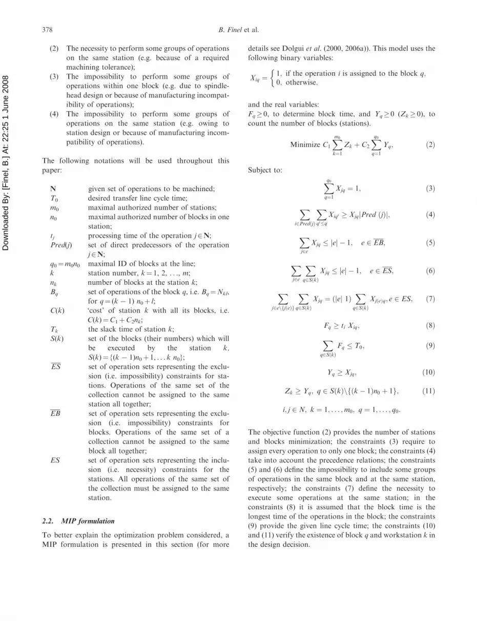
The problem can be illustrated by the following industrial

example. The workpiece to be manufactured is shown in

figure 2.

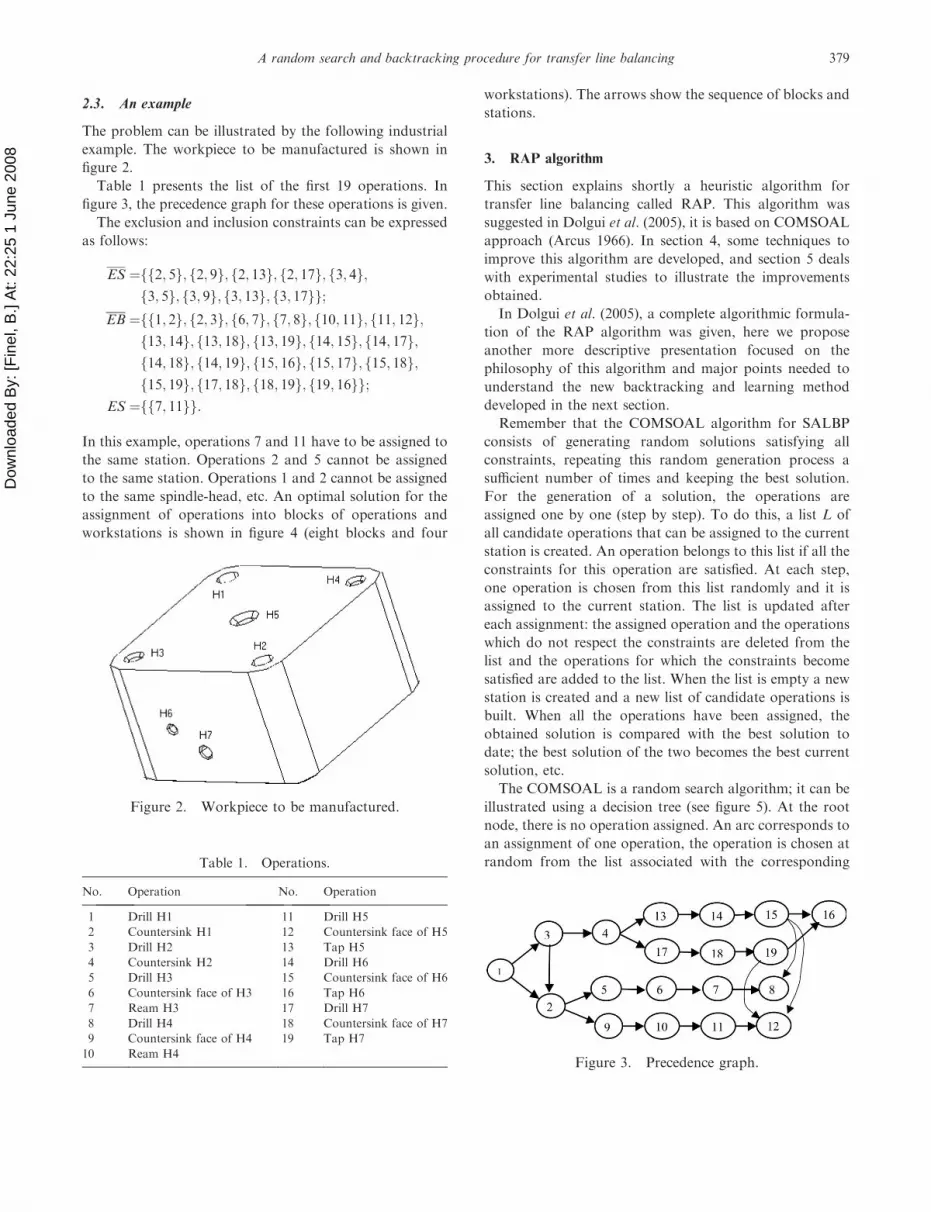
Table 1 presents the list of the first 19 operations. In

figure 3, the precedence graph for these operations is given.

The exclusion and inclusion constraints can be expressed

as follows:

ES ¼ f2; 5g; f2; 9g; f2; 13g; f2; 17g; f3; 4g;ff3; 5g; f3; 9g; f3; 13g; f3; 17gg;

EB ¼ f1; 2g; f2; 3g; f6; 7g; f7; 8g; f10; 11g; f11; 12g;ff13; 14g; f13; 18g; f13; 19g; f14; 15g; f14; 17g;f14; 18g; f14; 19g; f15; 16g; f15; 17g; f15; 18g;f15; 19g; f17; 18g; f18; 19g; f19; 16gg;

ES ¼ f7; 11gf g:

In this example, operations 7 and 11 have to be assigned to

the same station. Operations 2 and 5 cannot be assigned

to the same station. Operations 1 and 2 cannot be assigned

to the same spindle-head, etc. An optimal solution for the

assignment of operations into blocks of operations and

workstations is shown in figure 4 (eight blocks and four

workstations). The arrows show the sequence of blocks and

stations.

3. RAP algorithm

This section explains shortly a heuristic algorithm for

transfer line balancing called RAP. This algorithm was

suggested in Dolgui et al. (2005), it is based on COMSOAL

approach (Arcus 1966). In section 4, some techniques to

improve this algorithm are developed, and section 5 deals

with experimental studies to illustrate the improvements

obtained.

In Dolgui et al. (2005), a complete algorithmic formula-

tion of the RAP algorithm was given, here we propose

another more descriptive presentation focused on the

philosophy of this algorithm and major points needed to

understand the new backtracking and learning method

developed in the next section.

Remember that the COMSOAL algorithm for SALBP

consists of generating random solutions satisfying all

constraints, repeating this random generation process a

sufficient number of times and keeping the best solution.

For the generation of a solution, the operations are

assigned one by one (step by step). To do this, a list L of

all candidate operations that can be assigned to the current

station is created. An operation belongs to this list if all the

constraints for this operation are satisfied. At each step,

one operation is chosen from this list randomly and it is

assigned to the current station. The list is updated after

each assignment: the assigned operation and the operations

which do not respect the constraints are deleted from the

list and the operations for which the constraints become

satisfied are added to the list. When the list is empty a new

station is created and a new list of candidate operations is

built. When all the operations have been assigned, the

obtained solution is compared with the best solution to

date; the best solution of the two becomes the best current

solution, etc.

The COMSOAL is a random search algorithm; it can be

illustrated using a decision tree (see figure 5). At the root

node, there is no operation assigned. An arc corresponds to

an assignment of one operation, the operation is chosen at

random from the list associated with the corresponding

Figure 2. Workpiece to be manufactured.

Table 1. Operations.

No. Operation No. Operation

1 Drill H1 11 Drill H5

2 Countersink H1 12 Countersink face of H5

3 Drill H2 13 Tap H5

4 Countersink H2 14 Drill H6

5 Drill H3 15 Countersink face of H6

6 Countersink face of H3 16 Tap H6

7 Ream H3 17 Drill H7

8 Drill H4 18 Countersink face of H7

9 Countersink face of H4 19 Tap H7

10 Ream H4Figure 3. Precedence graph.

A random search and backtracking procedure for transfer line balancing 379

Dow

nloa

ded

By:

[Fin

el, B

.] A

t: 22

:25

1 Ju

ne 2

008

father node. One complete branch in this tree gives a

solution. To find the next solution (i.e. to make the next

iteration), the algorithm goes up to the root node. The

nodes illustrated by a rhombus in figure 5 represent the

cases when a station is closed (i.e. its maximum number of

operations is reached) and a new station is opened.

The RAP algorithm is inspired from the COMSOAL

method, but it takes into account specific constraints and

characteristics of the transfer line balancing problem which

is more complex: blocks of parallel operations, special type

of precedence constraints, inclusion and exclusion con-

straints, costs of blocks and stations, etc.

Remember that the following notations are used in this

paper:

C(k) is the cost of station k including the cost of its

blocks;

Tk is the slack time of station k (see below);

qk is the number of blocks for station k;

Bq is the set of operations of block q.

As with COMSOAL, the RAP algorithm uses a list L,

which groups all the operations that can be assigned to the

current station. For each state of the RAP algorithm, L

contains an operation i if:

1. The processing time ti is lower than the slack

time Tk of the current station k, i.e.:

ti � Tk ¼ T0 �P

q02SðkÞnfqg Fq0 ;

where q is the current block ID and Fq is the

duration of the block q;

2. Exclusion constraints ES can be satisfied (also

taking into account all the operations already

assigned to the current station);

3. All their predecessors are either already assigned or

are in L.

One particularity of the considered problem is that the

operations linked by precedence constraints can stay

Figure 4. An optimal solution for the example.

Figure 5. A decision tree for the COMSOAL method.

380 B. Finel et al.

Dow

nloa

ded

By:

[Fin

el, B

.] A

t: 22

:25

1 Ju

ne 2

008

together in the list of candidate operations (i.e. an

operation and its predecessors can be found together

in L). This is due to the previously mentioned specificity of

the precedence constraints and also to the grouping of the

operation in blocks.

The RAP algorithm can also be considered as a random

search in a decision tree. The root node defines the

beginning of the algorithm (no operation is assigned).

Each arc means the assignment of one operation to

the current block (of the current station). Each node of

the enumeration tree is characterized by the set of the

operations already assigned. The branching is linked with

the choice of one operation to be assigned among all

candidate operations from L. Each leaf of the tree for

which the set of assigned operations is the set N gives a

complete solution.

A particularity of RAP is that an additional type of node

must be used: the nodes which represent the case when a

block is closed. This type of node will be represented by a

rectangle. Another specificity is linked to the fact that some

iterations can be non-conclusive, i.e. a branch must be

stopped owing to a conflict between some constraints.

When an iteration is finished (conclusive or non conclu-

sive), the next iteration begins from the root node. The non

conclusive iteration is ignored.

In other words, if one branch is covered until all the

operations are assigned, respecting all the constraints, a

solution is found; if no more operation can be added to the

branch among non assigned operations, the iteration is

considered as non-conclusive and a new iteration (from the

root of the tree) begins.

At each iteration of the RAP algorithm, one operation is

chosen at random in L to be assigned to the current block.

If this operation has some predecessors in L, then the

predecessors are assigned first. When an operation must be

assigned, all operations present with this operation in a set

e2ES has to be assigned together.

For each candidate operation, if this operation cannot

be assigned to the current block, then a new block is

created for the current station. If the slack time or ES

constraints prohibit the creation of a new block for the

current station, then a new station is created. When a

station is closed, the constraints ES are verified.

When there is a subset of operations from a set e2ESnot assigned to this station when other operations from

the same set e are assigned, then this is a non-feasible

solution (the iteration is stopped, it is considered as non

conclusive).

When an operation is assigned, L is updated (the

assigned operation is deleted and the operations which

become available are added). A conclusive iteration of this

algorithm gives a feasible solution for the transfer line.

The RAP algorithm gives good results but leads to many

non-conclusive iterations (iterations with non feasible

solutions). To increase its performance, a backtracking

procedure is developed in the next section.

4. The BAL (backtracking and learning) procedure

4.1. General approach

The RAP algorithm can be interpreted as a random search

in the decision tree, so an efficient backtracking procedure

can improve its performance. Note that a heuristic of this

type for the simple assembly line balancing problem

(MALB) has been developed by Dar-El (1973) and showed

its performance.

The BAL method will be explained using a decision tree,

where a list L is associated to each node (this list gives the

number of possible branches). The BAL method allows

going back in the decision tree from node to predecessor

node: this is the backtracking effect. Only nodes which

represent closed blocks (no more operations can be added

to these blocks) are used in backtracking (i.e. a step of

backtracking consists of going up the previous block).

The branches where good solutions were found are

preferred to those where failures (non conclusive iterations

or solutions with a bad performance) occurred: this is the

learning mechanism. The better the solution obtained, the

smaller is the probability to cancel a block on this branch in

the backtracking procedure (i.e. the bigger is the prob-

ability to stop the backtracking at earlier steps).

The following additional notations are used for the

parameters needed to describe the BAL algorithm:

Nb minimum number of levels (blocks) in the

decision tree to backtrack;

Random a variable uniformly distributed between

0 and 1;

Prob probability to not backtrack to the

precedent level;

ProbInit algorithm parameter giving the initial

value of Prob;

Nlevel counter of the number of backtracked

levels;

NdblInit parameter giving the maximum author-

ized number of trials to build a block;

Ndbl counter of the number of trials;

CovTree parameter allowing the calculation of

the maximal number of authorized

branching;

Nbra(v) maximal number of authorized branching

from the vertex v;

Level(v) order of the last operation in the assign-

ment sequence from the root to v;

Weight(i) the probability to be chosen for the

operation i;

Coef1, Coef2 model parameters.

A random search and backtracking procedure for transfer line balancing 381

Dow

nloa

ded

By:

[Fin

el, B

.] A

t: 22

:25

1 Ju

ne 2

008

4.2. Some techniques used in BAL

The RAP algorithm is run. Each time a block is closed, a

decision is made: either the partial solution is kept and the

next block (or station) is opened and the RAP algorithm

continues, or a backtracking is executed due to the fact that

the end of the branch is reached. The end of the branch is

reached (i.e. the current iteration is terminated) if:

(a) either, the lower bound (LB) of the current node is

greater than the criterion value for the best solution

at this step (upper bound–UB); it is then sure that,

if the search in the branch goes on, the final

solution (when all the operations are assigned) will

be worse than UB (the iteration is stopped);

(b) or, all the operations are not assigned but no other

operation can be add to the current branch while

respecting the constraints (the iteration is not

conclusive, it is stopped);

(c) or, all the operations are assigned, i.e. a feasible

solution is found (the iteration is conclusive).

Each time there is a backtracking and the algorithm RAP

restarts from a node after backtracking, there is a new

iteration. In the first case above (LB4UB), the next

iteration is started from the root of the decision tree

independent of the node where the algorithm stopped

(backtracking up to root automatically). For the second

(non conclusive) and third (conclusive) cases, some specific

BAL techniques are proposed. The general schema of

algorithm is presented in figure 6.

4.3. Backtracking

The goal of backtracking is to keep a part of the current

solution for the next iteration; because this iteration can go

quicker than the one began at the root of the tree: some

operations already assigned (using good decisions) have to

Figure 6. Branching and backtracking scheme with BAL.

382 B. Finel et al.

Dow

nloa

ded

By:

[Fin

el, B

.] A

t: 22

:25

1 Ju

ne 2

008

be kept. The backtracking is done with a probability. The

reuse probability should depend on the quality of this

branch. The better the solutions on this branch, the sooner

it is necessary stopping going up (more blocks of the last

decision are involved again). The algorithm climbs up the

current branch block by block (it is not useful to stop at

each node but only where a block has been closed). At one

node, a decision to stop going up is made: a new branch is

started from there.

The Nb parameter gives the minimum number of levels

to go up (minimal number of blocks to cancel), for a

complete solution, to continue branching. In fact, it is

necessary to go up to a minimum of two blocks for a

complete solution to go back to a state from where a

different solution than the precedent one can be obtained.

The end user must be allowed to set the value of the

parameter Nb by fixing it greater or equal to 2 (i.e. Nb� 2).

Note that this parameter is applied only for a complete

solution, for a partial solution (i.e. for the case of a non-

conclusive iteration), only one block is cancelled.

A value of the variableRandom is generated between 0 and

1. If Random� (17Prob) and if the root has not been

reached, the algorithmgoes upone level in the tree, newvalue

ofRandom is generated and so on, otherwise a newbranching

starts. The probability Prob introduces a random choice to

have the possibility to go up onemore level. There is only one

variable Prob in the algorithm because only one branch is

treated at the same time. The initial value of Prob is given by

ProbInit, which is a parameter of the algorithm. Each new

feasible solution obtained by the algorithm changes the

current value of Prob. The better the obtained solution,

the higher is the increase of the probabilityProb. Conversely,

the worse the current solution, the lower is the new value

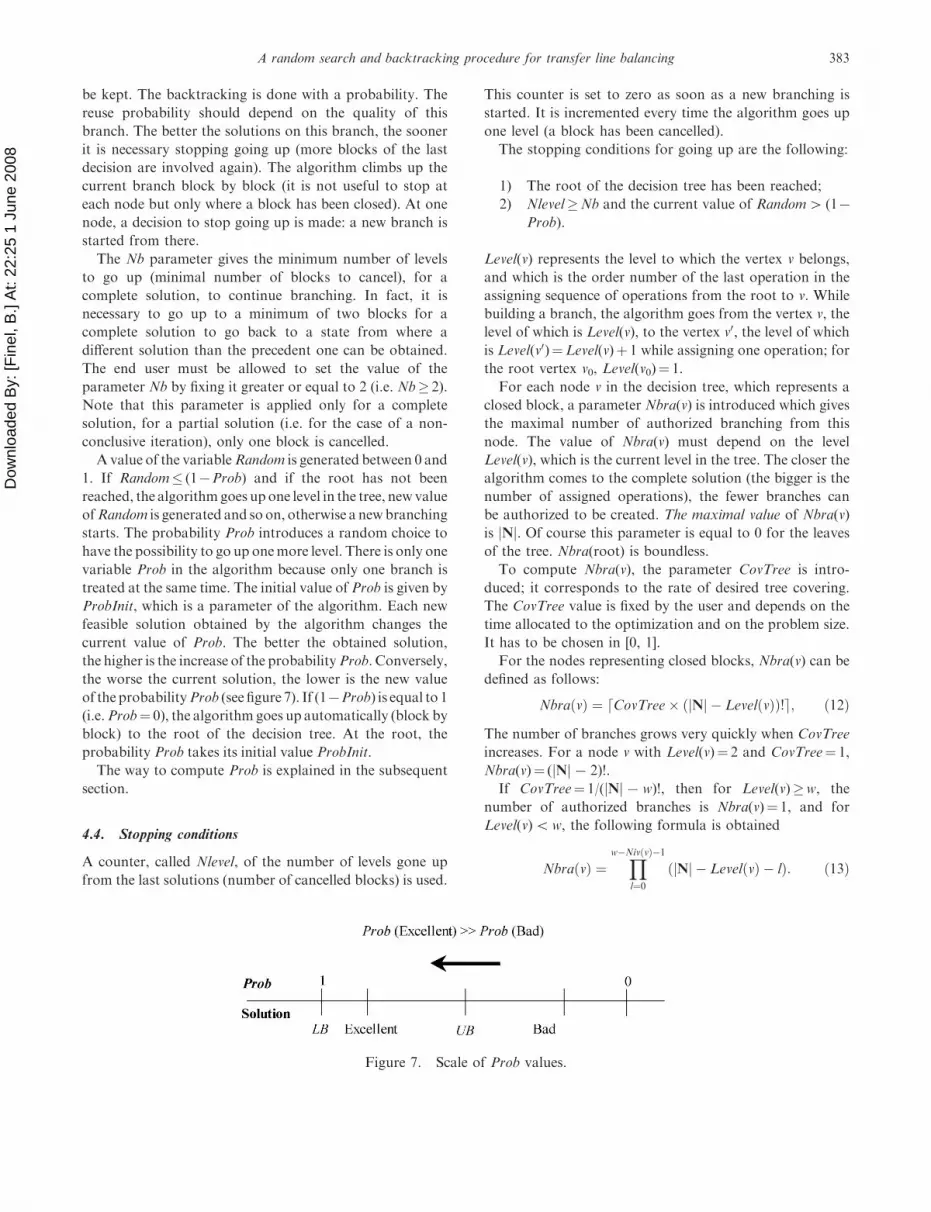
of the probabilityProb (see figure 7). If (17Prob) is equal to 1

(i.e.Prob¼ 0), the algorithm goes up automatically (block by

block) to the root of the decision tree. At the root, the

probability Prob takes its initial value ProbInit.

The way to compute Prob is explained in the subsequent

section.

4.4. Stopping conditions

A counter, called Nlevel, of the number of levels gone up

from the last solutions (number of cancelled blocks) is used.

This counter is set to zero as soon as a new branching is

started. It is incremented every time the algorithm goes up

one level (a block has been cancelled).

The stopping conditions for going up are the following:

1) The root of the decision tree has been reached;

2) Nlevel�Nb and the current value of Random4 (17Prob).

Level(v) represents the level to which the vertex v belongs,

and which is the order number of the last operation in the

assigning sequence of operations from the root to v. While

building a branch, the algorithm goes from the vertex v, the

level of which is Level(v), to the vertex v0, the level of which

is Level(v0)¼Level(v)þ 1 while assigning one operation; for

the root vertex v0, Level(v0)¼ 1.

For each node v in the decision tree, which represents a

closed block, a parameter Nbra(v) is introduced which gives

the maximal number of authorized branching from this

node. The value of Nbra(v) must depend on the level

Level(v), which is the current level in the tree. The closer the

algorithm comes to the complete solution (the bigger is the

number of assigned operations), the fewer branches can

be authorized to be created. The maximal value of Nbra(v)

is jNj. Of course this parameter is equal to 0 for the leaves

of the tree. Nbra(root) is boundless.

To compute Nbra(v), the parameter CovTree is intro-

duced; it corresponds to the rate of desired tree covering.

The CovTree value is fixed by the user and depends on the

time allocated to the optimization and on the problem size.

It has to be chosen in [0, 1].

For the nodes representing closed blocks, Nbra(v) can be

defined as follows:

NbraðvÞ ¼ CovTree� jNj � LevelðvÞð Þ!d e; ð12Þ

The number of branches grows very quickly when CovTree

increases. For a node v with Level(v)¼ 2 and CovTree¼ 1,

Nbra(v)¼ (jNj7 2)!.

If CovTree¼ 1/(jNj7w)!, then for Level(v)�w, the

number of authorized branches is Nbra(v)¼ 1, and for

Level(v)5w, the following formula is obtained

NbraðvÞ ¼Yw�NivðvÞ�1

l¼0jNj � LevelðvÞ � lð Þ: ð13Þ

Figure 7. Scale of Prob values.

A random search and backtracking procedure for transfer line balancing 383

Dow

nloa

ded

By:

[Fin

el, B

.] A

t: 22

:25

1 Ju

ne 2

008

When a new node representing a block is created, the initial

value of Nbra(v) is computed according to equation (13).

For each branching from the vertex v, the value of the

Nbra(v) parameter is decremented as follows: Nbra(v)¼Nbra(v)7 1. When Nbra(v)¼ 0, the stopping condition is

reached (there is no more possibility to build a new branch

from this vertex v), the algorithm goes one block up. At the

root, Nbra(v0)¼�.

4.5. Probability to choose an operation

When a node v is reached, the corresponding list of

candidate operations L is established from which an

operation to be assigned is randomly chosen. Initially,

the weight (and in consequence the probability to be

chosen) is the same for each operation in L: it is equal to

1, i.e. Weight1i¼ 1, where the superior index gives

the current branching number, the inferior index represents

the operation number. In other words, the superior

index gives the number of times that this node has been

found in the current iteration. It grows any time the

algorithm passes again by this node. When the algorithm

stops at a node while going up, it does again a random

branching. To avoid generating the same branch, the

weight of candidate operations is modified. This is made

when a block is closed. In this case, the operation which

closes the block is known and it is desired to have in the

future less chance to choose it, so a smaller value is given to

its weight.

Weightlj¼ Coef1� Prob�Weightl�1

j; ð14Þ

where Coef1 is a model parameter 0�Coef1� 1.

After the modification of the operation j weight, the

probability to be chosen for the operation j is normalized

and is equal to:

pj ¼WeightjPl2L Weightl

: ð15Þ

4.5.1. Non-conclusive iteration treatment. A particular

treatment is added for the non-conclusive iterations. When

iteration is non-conclusive (blocking), it is necessary to go

one block up and to change the weight of all the candidate

operations from L. The weight of all the operations of the

last closed block (and not only of one operation as before)

must be modified as follows:

Weightli¼ Coef2�Weightl�1

i; ð16Þ

where Weightliis the weight of the operation i for the lth

trial to obtain a conclusive iteration, Weight1i¼ 1, Coef2 is

a coefficient (parameter) of the model, 0�Coef2� 1; i2L.

The obtained weights of operations are copied in all the

descending vertexes until a new station is created (for which

all the constraints are respected).

To avoid an infinite loop, a new parameter NdblInit and

a counter Ndbl are introduced. NdblInit gives a maximum

number of trials. The counter Ndbl is set to zero, when a

failure (non-conclusive) is established. It is incremented at

each new trial. When the counter Ndbl is equal to

NdblInit, the trials are stopped and the algorithm begins

to go up in the tree following the procedure of the

previous section.

4.5.2. Learning (computing of the probability Prob). The

learning technique is based on the calculation of the

probability Prob characterizing the branch quality. If Prob

is equal to 1, then the algorithm stops, an optimal solution

is founded. If Prob is lower than one, then the algorithm

goes block by block up in the decision tree, each time with

the probability (1-Prob). Consequently, Prob must signifi-

cantly reduce if the iteration is of bad quality or stopped, or

in the case of blocking (non-conclusive iteration); it must

increase in case of good iteration. The positive increasing

must be proportional to the solution quality.

To compute Prob, the upper bounds (initial UB0 and

running UB) and lower bounds (initial LB0 and running

local LLB) of the objective function are used. The

difference between the initial bounds UB0 and LB0

corresponds to an estimation of the maximum distance

(DstMax) between the solutions

DstMax ¼ UB0 � LB0: ð17Þ

The initial upper bound UB0 is equal to

UB0 ¼ C1 m0 þ C2 q0: ð18Þ

The initial lower bound LB0 is equal to

LB0 ¼ C1mþ C2n ¼ C1 maxi2N

k�½i�ð Þ

þ C2 maxi2N

q�½i�jn0 ¼ 1;ES ¼ f;gð Þ:ð19Þ

where k7 [i] and q7[i] are the lower bounds of possible

indices for workstation and blocks, respectively, where the

operation i can be assigned (in Dolgui et al. (2006a)

the corresponding pre-processing procedure tacking into

account all the problem constraints and the methods to

compute k7 [i], q7[i], kþ [i] and qþ[i]). For example, if an

operation i cannot be in the same block as the operation j

and it precedes the operation j, then if the smallest block

where i can be assigned is equal to q7[i] then the smallest

block where j can be assigned is q7[j]4 q7[i].

If a branch is not running to the end (all the operations

are not already assigned), then there is a partial solution

384 B. Finel et al.

Dow

nloa

ded

By:

[Fin

el, B

.] A

t: 22

:25

1 Ju

ne 2

008

p with N \N assigned operations. For this solution, the

criterion C(p) is equal to:

CðpÞ ¼ C1 mðpÞ þ C2 nðpÞ;

where m(p) and n(p) are the number of stations and the

number of blocks, respectively.

To obtain a local lower bound, LLB for p, after having

assigned a set of operations N, it is necessary to fix

q�p ½j� ¼ qþp ½j� ¼ q½j� and k�p ½j� ¼ kþp ½j� ¼ k½j�, for j2N and to

compute again q�p ½i� and k�p ½i� for i2N\N using the same

algorithm (see Dolgui et al. 2006a). Here, qp[j] and kp[j] are

the numbers of blocks and stations for the operation j in

the partial solution p and where k�p ½i� and q�p ½i� are the

lower bounds of possible indices for workstation and

blocks, respectively, where the operation i is in the partial

solution p

LLB ¼ C1 maxi2N

k�p ½i�� �

þ C2 maxi2N

q�p ½i�jn0 ¼ 1; ES ¼ f;g� �

;ð20Þ

When all the operations of N are assigned, there is a

complete feasible solution P

CðpÞ ¼ C1 mþ C2 n:

As soon as the new value of the criterion is better than the

current upper bound UB, it becomes the new current UB.

There are four different cases for probability Prob

calculation:

1. If LLB�UB, i.e. the local lower bound for the

partial solution p is greater or equal to the best

complete solution found then the iteration is

stopped, Prob¼ 0 (17Prob¼ 1), the algorithm goes

block by block up to the root.

2. If there is no possibility to assign operations due to

the constraints (a non-conclusive iteration), the

value of Prob is corrected while decreasing it in

such a manner

Probs ¼ Probs�1 � Probs�1 1� UB� LLB

UB0 � LB0

� �: ð21Þ

3. If a feasible solution is found but without getting a

better value for the current upper bound, then

Probs ¼ Probs�1 � Probs�1CðPÞ �UB

UB0 �UB

� �: ð22Þ

If C(P)¼UB0, Prob¼ 0 (17Prob¼ 1), the algorithm goes

block by block up to the root, this is also considered as

valid for the rare cases when UB¼UB0.

4. If a good solution is found (all the operations are

assigned and the criterion is better than the current

UB), then

Probs ¼ Probs�1 þ ð1� Probs�1ÞUB� CðPÞUB� LB0

: ð23Þ

If C(P)¼LB0, Prob¼ 1 (17Prob¼ 0), then the algorithm

stops, the optimal solution is found.

5. Experimental results

Tests were carried out on a Compaq W6000 bi-processor

machine, Intel Xeon with 1.70 Ghz for central processing

unit (CPU) and 1 Giga RAM.

The parameters of 15 studied examples are given in

table 2. The examples with numbers from 3 to 16

(12 examples) were generated randomly; they are the same

as those in Dolgui et al. (2005) with the same example

numbers. The last three examples (i1, i2 and i3) are

additional small industrial examples. The following nota-

tions are used:

EX the example number,

NO the number of operations,

NA the number of arcs in the precedence digraph,

nEB the tg number of subsets in EB,

nES the number of subsets in ES,

nES the number of subsets in ES,

rEB the max dimension for the subsets of EB,

rES the max dimension for the subsets of ES,

rES the max dimension for the subsets of ES.

The parameter values for the BAL algorithm have been

chosen in the following manner: several runs of the

algorithm are made. For each run, ten different values of

a parameter are given (fixing the others). After these runs,

the values which gave the best results for each parameter

are kept and then the algorithm is run again. Some

examples of the parameters assigned are given in table 3.

Table 4 presents the experimental results for all test

examples. The first column gives the number of operations,

the second and third ones give the constraints on the

maximal number of blocks for one station and on the

maximal number of stations allowed. Then, the next

column shows the optimal solution (for the examples from

3 to 10 and for i1, i2 and i3 we have an optimal solution

obtained with the model (2)–(11) and ILOG Cplex solver).

The next column gives the solutions obtained with RAP

and BAL, and the last two columns present CPU times.

The stop condition for both RAP and BAL was the number

of iterations equal to 10 000.

The utilization of BAL with RAP allows us to reach very

quickly the optimal value for the criterion (this optimal

A random search and backtracking procedure for transfer line balancing 385

Dow

nloa

ded

By:

[Fin

el, B

.] A

t: 22

:25

1 Ju

ne 2

008

value is also obtained using MIP model with Cplex solver)

for small examples. The criterion value is optimal and it

was reached for both methods.

For all examples except for example 15 with 100

operations the solution of RAP and BAL are the same,

but the calculation time is different. The solution obtained

with BAL for the example with 100 operations is better.

The results given in table 4 were obtained for 10 000

iterations of each algorithm. Table 5 shows the results for

the example with 100 operations, where these algorithms

Table 2. Parameters of the test examples.

EX NO NA nEB nES nES m0 n0 T0 rEB rES rES

3 11 11 2 1 1 6 3 9 2 3 2

4 13 17 3 3 2 4 3 11 3 2 3

5 15 15 5 1 1 4 3 7 2 3 2

6 17 25 4 3 3 4 3 12 3 3 2

7 18 26 3 3 3 5 3 15 2 3 3

8 23 39 4 4 3 4 4 50 3 3 3

9 25 38 3 3 3 6 3 16 3 3 3

10 29 44 3 4 4 6 3 80 3 3 2

11 35 46 12 4 5 20 20 70 4 5 4

13 38 62 4 6 5 7 3 20 2 2 3

14 45 67 5 4 4 7 3 100 3 3 3

15 100 194 6 7 5 7 3 35 2 2 3

16 120 214 14 7 8 7 3 27 4 2 3

i1 9 19 12 8 – 6 2 200 2 2 –

i2 17 51 47 9 – 3 9 300 2 2 –

i3 15 52 35 34 – 3 8 400 2 2 –

Table 3. Parameters and results for RAP and RAPþBAL.

EX NO

Parameters Criterion value CPU time

1/CovTree Coef1 Coef2 NdblInit ProbInit RAP RAPþBAL RAP RAPþBAL

3 11 360 0.75 0.35 6 0.65 36 (3,3) 26 (2,3) 30 0.010

4 13 660 0.75 0.35 6 0.65 36 (3,3) 36 (3,3) 360 0.010

5 15 24 024 0.7 0.5 6 0.5 36 (3,3) 36 (3,3) 550 0.020

11 35 33 390 720 0.7 0.5 6 0.5 52 (4,6) 40 (3,5) 20 0.830

14 45 130 320 960 0.7 0.4 9 0.7 54 (4,7) 42 (3,6) 10040 110

Table 4. Experimental results.

EX NO Optimum ILOG Cplex Solution RAP Solution RAPþBAL

CPU time

RAP RAPþBAL

3 11 26 (2,3) 36 (3,3) 26 (2,3) 30 0.010

4 13 36 (3,3) 36 (3,3) 36 (3,3) 40 0.010

5 15 24 (2,2) 24 (2,2) 24 (2,2) 50 0.020

6 17 36 (3,3) 36 (3,3) 36 (3,3) 70 0.020

7 18 40 (3,5) 52 (4,6) 40 (3,5) 70 0.030

8 23 40 (3,5) 40 (3,5) 40 (3,5) 90 0.060

9 25 38 (3,4) 40 (3,5) 40 (3,5) 210 0.060

10 29 38 (3,4) 48 (4,4) 38 (3,4) 30 0.030

11 35 – 54 (4,7) 40 (3,5) 460 0.830

13 38 52 (4,6) 54 (4,7) 54 (4,7) 150 0.180

14 45 – 54 (4,7) 42 (3,6) 100400 110

15 100 – 82 (6,11) 68 (5,9) 20900 160

16 120 – 54 (4,7) 54 (4,7) 403000 150

i1 9 42 (3,6) 42 (3,6) 42 (3,6) 30 10

i2 17 30 (2,5) 30 (2,5) 30 (2,5) 30 0.40

i3 15 44 (3,7) 44 (3,7) 44 (3,7) 50 0.50

386 B. Finel et al.

Dow

nloa

ded

By:

[Fin

el, B

.] A

t: 22

:25

1 Ju

ne 2

008

have been run from 10 000 to 60 000 with a step of 10 000

iterations. The first column gives the number of iterations;

the two following columns present the two criterion values

(one for each algorithm) then follow the CPU times.

6. Conclusion

A crucial step of machining line design was considered. It

concerns the logical layout design, i.e. the logical synthesis

of the manufacturing process, which consists of grouping

the operations into blocks (spindle-heads) and the blocks

into stations. An error at this step (or an inefficient

solution) drastically increases the line and machining

product costs. Therefore, the development of decision

support methods and tools for logical layout design of this

type of machining line is a challenging perspective.

An original approach was suggested in this paper. It

deals with the mathematical modelling of the considered

problem and with the search of a good and if possible

optimal solution of this model, minimizing the number

pieces of equipment (spindle heads, stations) and consecu-

tively the line cost.

A new heuristic algorithm to find a ‘good’ design

decision has been presented in this paper. This heuristic is

an extension of the COMSOAL-based method RAP. To

develop this extension, the problem has been presented as a

problem of random search in a decision tree. An efficient

approach to explore this decision tree has been proposed. It

uses several techniques of backtracking and learning. The

goal of backtracking is to keep a part of the current

solution for the next iteration; because this iteration can go

quicker than the one began at the root of the tree: some

operations already assigned (using good decisions) have to

be kept. The backtracking is done with a probability:

the better the solution obtained, the smaller should be the

probability to cancel a block on this branch in the

backtracking procedure. These techniques were developed

in detail in this paper.

The results of tests are promising. The employment of

the proposed techniques drastically improves the heuristic

RAP, decreasing the CPU times and giving better results

from the criterion value point of view for the problems

tested.

The perspectives of our research consist of an analysis of

the suggested algorithm parameters. These parameters have

to be adjusted and tested to reach better results. It is also

interesting to produce more test results to study the

behaviour of the developed techniques and to find new

ways to increase the algorithm calculation efficiency and

results.

Acknowledgements

The authors thank Dr N. Guschinsky and Professor G.

Levin for discussions, help and data for the industrial cases

of this problem.

References

Arcus, A.L., COMSOAL: a computer method of sequencing operations for

assembly lines. Int. J. Prod. Res., 1966, 4, 259–277.

Baybars, I., A survey of exact algorithms for the simple assembly line

balancing. Mgmt Sci., 1986, 32.

Boctor, F.F., A multiple-rule heuristic for assembly line balancing. J. Opl

Res. Soc., 1995, 46, 62–69.

Dar-El, E.M., MALB – a heuristic technique for balancing large single-

model assembly lines. AIIE Trans., 1973, 5, 343–356.

Dashchenko A.I. (editor) Manufacturing Technologies for Machines of the

Future 21st Century Technologies, 2003 (Springer: New York).

Dolgui, A., Guschinsky, N. and Levin, G., Approaches to Balancing of

Transfer Line with Block of Parallel Operations. Institute of Engineering

Cybernetics/University of Technology of Troyes, Minsk, Preprint No. 8,

2000.

Dolgui, A., Finel, B., Guschinsky, N., Levin, G. and Vernadat, F., MIP

approach to balancing transfer lines with blocks of parallel operations.

IIE Trans., 2006a, 38, 869–882.

Dolgui, A., Finel, B., Guschinskaya, O., Guschinsky, N., Levin, G. and

Vernadat, F., Balancing large-scale machining lines with multi-spindle

heads using decomposition. Int. J. Prod. Res., 2006b, 44, 4105–4120.

Dolgui, A., Guschinsky, N., Levin, G. and Proth, J.-M., Optimisation of

multi-position machines and transfer lines. Eur. J. Opl Res., 2006c.

Accepted, in press.

Dolgui, A., B. Finel, N. Guschinsky, G. Levin, F. Vernadat, An heuristic

approach for transfer lines balancing. J. Intell Mfg., 2005, 16, 159–172.

Erel, E. and Sarin, S.C., A survey of the assembly line balancing

procedures. Prod. Planning and Control, 1998, 9, 414–434.

Ghosh, S. and Gagnon, R., A comprehensive literature review and analysis

of the design, balancing and scheduling of assembly lines. Int. J. Prod.

Res., 1989, 27, 637–670.

Groover, M.P., Automation. Production Systems and Computer Integrated

Manufacturing, 1987 (Prentice Hall: Englewood Cliffs, New Jersey).

Hitomi, K., Manufacturing Systems Engineering, 1996 (Taylor & Francis:

Abingdon).

Martin, P. and D’Acunto, A., Design of a production system: an

application of integration product-process. Int. J. Comput. Integr.

Mfg., 2003, 16, 509–516.

Rekiek, B., Dolgui, A., Delchambre, A. and Bratcu, A., State of the art of

assembly lines design optimisation. Ann. Rev. Control, 2002, 26, 163–174.

Scholl, A. and Klein, R., Balancing assembly lines effectively: a

computational comparison. Eur. J. Opl Res., 1998, 114, 51–60.

Talbot, F.B., Patterson, J.H. and Gehrlein, W.V., A comparative

evaluation of heuristic line balancing techniques. Mgmt Science, 32,

430–454.

Table 5. Comparison RAP and RAPþBAL for the examplewith 100 operations.

Number of iterations

Criterion CPU time

RAP RAPþBAL RAP RAPþBAL

6000 82 82 10520 140

10 000 82 68 20900 160

20 000 82 68 20280 220

60 000 82 68 40380 1090

A random search and backtracking procedure for transfer line balancing 387