Backtracking and ProbingPaul Walton Purdom, Jr., Indiana UniversityG. Neil Haven, Indiana UniversityPartial support provided by NSF Grant CCR 92-03942.Abstract: We analyze two algorithms for solving constraint satisfaction problems. One of these algorithms,Probe Order Backtracking, has an average running time much faster than any previously analyzed algorithmfor problems where solutions are common. Probe Order Backtracking uses a probing assignment (a prese-lected test assignment to unset variables) to help guide the search for a solution to a constraint satisfactionproblem. If the problem is not satis�ed when the unset variables are temporarily set to the probing assign-ment, the algorithm selects one of the relations that the probing assignment fails to satisfy and selects anunset variable from that relation. Then at each backtracking step it generates subproblems by setting theselected variable each possible way. It simpli�es each subproblem, and tries the same technique on them.For random problems with v variables, t clauses, and probability p that a literal appears in a clause, theaverage time for Probe Order Backtracking is no more than vn when p � (ln t)=v plus lower order terms.The best previous result was p � p(ln t)=v. When the algorithm is combined with an algorithm of Francothat makes selective use of resolution, the average time for solving random problems is polynomial for allvalues of p when t � O(n1=3(v= ln v)2=3). The best previous result was t � O(n1=3(v= ln v)1=6). Probe OrderBacktracking also runs in polynomial average time when p � 1=v, compared with the best previous resultof p � 1=(2v). With Probe Order Backtracking the range of p that leads to more than polynomial time ismuch smaller than that for previously analyzed algorithms.1 BacktrackingThe constraint satisfaction problem is to determine whether a set of constraints over discrete variablescan be satis�ed. Each constraint must have a form that is easy to evaluate, so any di�culty in solving sucha problem comes from the interaction between the constraints and the need to �nd a setting for the variablesthat simultaneously satis�es all of the constraints.Constraint satisfaction problems are extremely common. Indeed, the proof that a problem is NP-complete implies an e�cient way to transform the problem into a constraint satisfaction problem. Most NP-complete problems are initially stated as constraint satisfaction problems. A few special forms of constraintsatisfaction problems have known algorithms that solve problem instances in polynomial worst-case time.However, for the general constraint satisfaction problem no known algorithm is fast for the worst case.When no polynomial-time algorithm is known for a particular form of constraint satisfaction problem,it is common practice to solve problem instances with a search algorithm. The basic idea of searching isto choose a variable and generate subproblems by assigning each possible value to the variable. In eachsubproblem the relations are simpli�ed by plugging in the value of the selected variable. This step ofgenerating simpli�ed subproblems is called splitting. If any subproblem has a solution, then the originalproblem has a solution. Otherwise, the original problem has no solution. Subproblems that are simpleenough (such as those with no unset variables) are solved directly. More complex subproblems are solved byapplying the technique recursively.If a problem contains the always false relation, then the problem has no solution. Simple Backtrackingimproves over plain search by immediately reporting no solution for such problems. Backtracking often savesa huge amount of time.2 ProbingThis paper considers two algorithms that are improvements over Simple Backtracking. Both algorithmsuse the idea of probing : if a �xed assignment to the unset variables solves the problem, no additionalinvestigation is needed. Our algorithms probe by setting each unset variable to false and testing to seewhether all relations simplify to true. The two probing algorithms are simple enough that it is possible toanalyze their average running time. 1

Our �rst algorithm,Backtracking with Probing, uses backtracking, probing, and no additional techniques.In particular, during splitting it always picks the �rst unset variable from a �xed ordering on the variables.Our second algorithm, Probe Order Backtracking, is more sophisticated in its variable selection. It has a�xed ordering on the variables and a �xed ordering on the relations. First, it checks that there are no alwaysfalse relations. If an always false relation is encountered, the problem is not satis�able and the algorithmbacktracks. Next, it checks to see if there is a currently selected relation. If there is no currently selectedrelation, it selects the �rst relation that evaluates to false under the probing assignment. (If all clausesevaluate to true then the probing assignment solves the problem.) Finally, the algorithm does splitting usingthe �rst unset variable of the selected relation.3 Probability ModelThe average number of nodes generated when solving randomly generated problems is one measureof the quality of a search algorithm. We use this measure where our random problems are formed by theconjunction of independently generated random clauses (the logical or of literals, where a literal is a binaryvariable or the negation of a binary variable). A random clause is generated by independently selecting eachliteral with a �xed probability, p. We use v for the number of variables, and t for the number of clauses. Forthe asymptotic analysis, both p and t are functions of v.Many algorithms have been analyzed with this random clause length model [3, 4, 7, 8, 12, 16, 18, 21, 22].Most of these analyses and a few unpublished ones are summarized in [17]. A few algorithms have also beenanalyzed with the �xed length model, where random problems consist of random clauses of �xed length [1,2, 14, 20]. This second probability model generates problems that are more di�cult to satisfy but perhapsmore like the problems encountered in practice. The second model leads to much more di�cult analyses.4 Summary of ResultsThis section summarizes the performance of Probe Order Backtracking and gives some intuition as towhy Probe Order Backtracking is fast. The simpler Backtracking with Probing Algorithm turns out toprovide no signi�cant improvement over previously analyzed algorithms, so we do not discuss it in greatdetail.This paper has contour plots showing the performance of probing algorithms. We also include contourplots for the approximate performance analyses of these algorithms. Each plot is for random problems with50 variables. The vertical axis shows p, the probability that a given literal appears in a clause, running from0.001 to 1 with ticks at 0.01 and 0.1. At p = 0:01 the average clause length for problems is 1. At p = 0:1the average clause length is 10 literals. The horizontal axis shows t, the number of clauses, running from2 to 250 with ticks at 10 and 100. When p is near 0 or 1 most problems are trivial. When p is low mostproblems are easy because they contain an empty clause; empty clauses are trivially unsatis�able. When pis high most problems are easy because any assignment of values to variables is a solution to most problems.The region of hard problems lies in the middle.In most cases the contours are shaped like elongated horseshoes (see Fig. 2). The area within a horseshoecontour represents problems that are more di�cult than the problems outside the contour. The outermostcontour shows where the average number of nodes is 50, the next inner one 502, next 503, and �nally 504.Running near the centerline of the horseshoes is a line that shows for each t that value of p that results inthe hardest problems (those with the largest number of nodes).In the less favorable cases the upper and lower branches of a contour do not meet (see Fig. 1). In thosecases the uppermost and lowermost lines show where there is an average of 50 nodes, the next inner pair502 nodes, and so on. Again the centerline shows the p value that results in the largest number of nodes.Occasionally one of the contours runs along one of boundaries (see Fig. 6). The contours do not alwaysextend to the right edge of the �gure due to di�culties with oating point over ow (see Fig. 1).Figure 1 is a contour plot of the average number of nodes generated by Backtracking with Probing.This plot show shows that Backtracking with Probing provides no signi�cant improvement over previouslyanalyzed algorithms [17].Figure 2 is a contour plot of the average number of nodes generated by Probe Order Backtracking. Inthis case the upper and lower contours join to form horseshoe shaped curves. Note that the region of hardproblems is considerably smaller for Probe Order Backtracking than for Backtracking with Probing. Except2

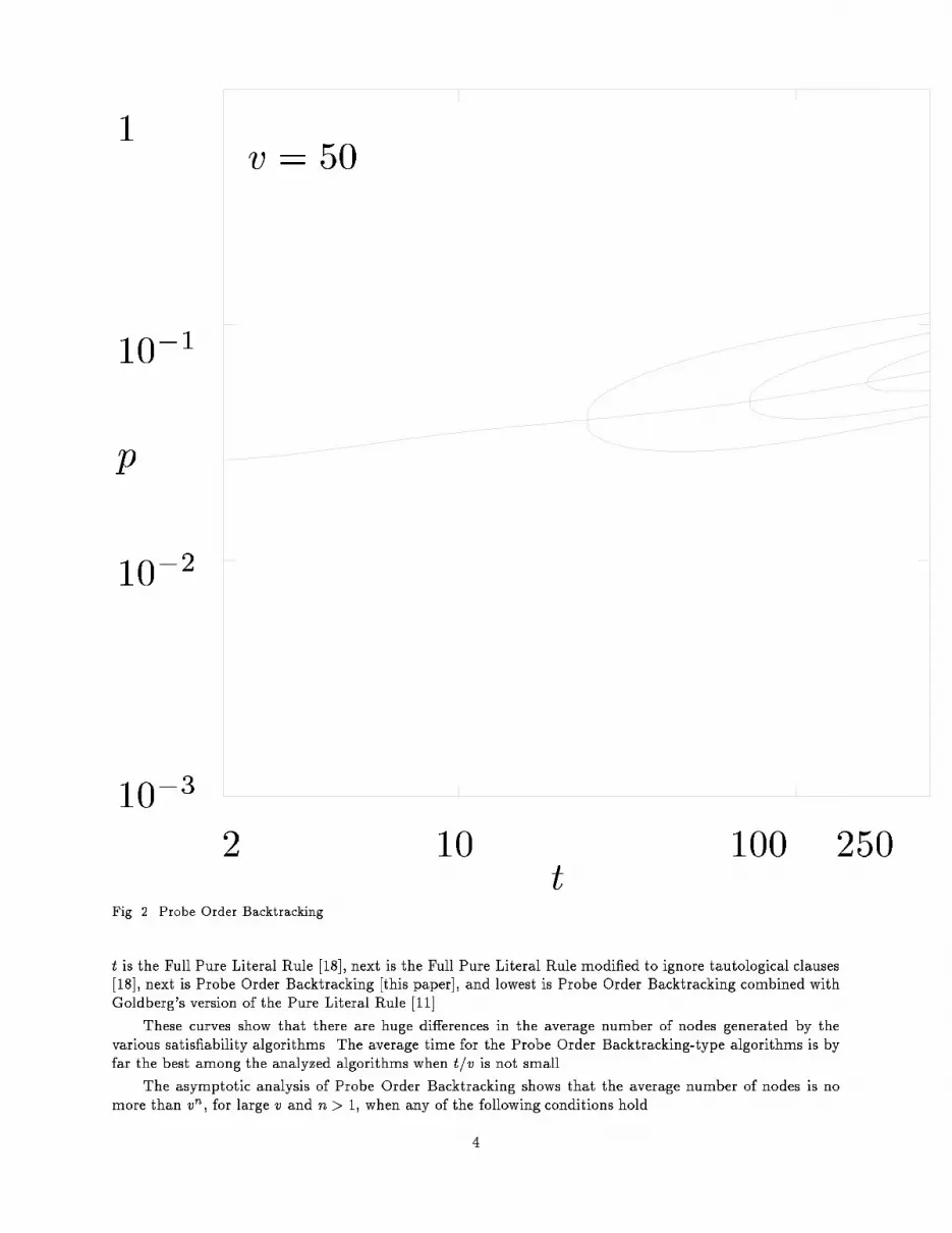
p110�110�210�3

v = 50

2 10 100 250tFig. 1. Backtracking with Probing.for the small t region, these contours are much better than those of any other algorithm for which suchcontours have been published. The improvement is particularly noticeable along the upper contour.Figure 3 shows how the average number of nodes for Probe Order Backtracking compares with theaverage for several other satis�ability algorithms when, for each value of t and each algorithm, p is set tomake the average as large as possible. The horizontal axis is the number of clauses (from 1 to 500 for thisgraph). The vertical axis is the average number of nodes from 1 to over 1015 with tick marks for each powerof 10. Of the curves that were computed to t = 500, the uppermost is Goldberg's simpli�ed version of thepure literal rule [9, 10], next is Clause Order Backtracking [3], and lowermost is backtracking combined withGoldberg's version of the pure literal rule [19]. Of the curves that stop short of t = 500 the highest for large3

p110�110�210�3

v = 50

2 10 100 250tFig. 2. Probe Order Backtracking.t is the Full Pure Literal Rule [18], next is the Full Pure Literal Rule modi�ed to ignore tautological clauses[18], next is Probe Order Backtracking [this paper], and lowest is Probe Order Backtracking combined withGoldberg's version of the Pure Literal Rule [11].These curves show that there are huge di�erences in the average number of nodes generated by thevarious satis�ability algorithms. The average time for the Probe Order Backtracking-type algorithms is byfar the best among the analyzed algorithms when t=v is not small.The asymptotic analysis of Probe Order Backtracking shows that the average number of nodes is nomore than vn, for large v and n > 1, when any of the following conditions hold4

1015

100

v = 50c

fpure

fpuret

p

b

probepureprobe

1 10 100 500tFig. 3. Worst p performance.p � ln t+ 2 ln ln t� ln ln v � ln(n� 1)� ln 2v +�� ln ln tv ln t � ; (1)p � � ln(t=v) + ln ln(t=v) + 1� ln 2� ln ln 22v �� �1 + 2(n � 1) lnv � (ln 2)[ln(t=v) + ln ln(t=v) + 3� ln 2� ln ln 2]4v ln 2��� (ln v) ln(t=v)v2 �� �� ln ln(t=v)v ln(t=v) ��; (2)5

p � 1v + e[(n � 1) lnv � ln 2]tv ; (3)t � (n� 1) lnv � ln 2lnf1 + [(pv)2 � 1]e�pv=2g : (4)The � term in bound (1) requires that t increases more rapidly than lnv. Bound (4) requires the assumptionthat the limit of pv is greater than 1 and �nite.By setting p to minimize the right side of (4) we see that for all p and large v, the average number ofnodes is no more than vn when t � 5:1150(n� 1) ln v ��(1): (5)Details: This sentence shows that you are reading the technical report. The extra details of thetechnical report are contained in sections starting with the word `details' and ending with a diamond.�Details: In bound (4) the minimum value of the right side (when considered as a function of pv) occursat pv = 1 +p2.�The bound for large p, bound (1), is much better than that for any previously analyzed algorithm. Thebest previous result was p �r ln t� lnnv (6)for Iwama's inclusion-exclusion algorithm [12]. In the region between bounds (1) and (6) Probe OrderBacktracking is the fastest algorithm with proven results on its running time. Algorithms that repeatedlyadjust variable settings to satisfy as many clauses as possible [24] are even faster on many problems. Thosealgorithms, however, have di�culty with problems which have no solution. They have been di�cult tocorrectly analyze, and it is not clear at this time what their average running time is.For the best previously analyzed algorithms there was a large range of p where the algorithms apparentlyrequired more than polynomial time. (The word apparently is used because the analyses were all upper boundanalyses.) The ratio of the large p boundary to the small p boundary was v1=2 times logarithmic factors.For Probe Order Backtracking, only the logarithmic factors are left. In some cases even the logarithmicfactors are gone and the ratio is constant (in the limit of large v). Bound (2) for small p results from thefact that the average number of nodes for Probe Order Backtracking is no larger than the average for SimpleBacktracking. When t = v� with � > 1, the ratio of the upper boundary (1) to the lower boundary (2) is2�=(�� 1) plus lower order terms. Thus, for large � only a very limited range of p leads to problems witha large average time.Perhaps the region of greatest interest is the one where t is proportional to v. When t is below 3:22135v,bound (3) is better than (2). When t = �v the ratio of the upper bound (1) to �rst lower bound (2) is(2 lnv)=(ln � + ln ln �+1� ln 2� ln ln 2) plus lower order terms. The ratio of the upper bound to the secondlower bound (3) is ln v plus lower order terms.Previously, for small t the best algorithm was a combination of Franco's limited resolution algorithm[8] for small p and Iwama's inclusion-exclusion algorithm [12] for large p. When p is unknown, the twoalgorithms can be run in parallel and stopped as soon as an answer is found. Each algorithm generates nomore than than vn nodes (regardless of p) when t = O(n1=3(v= ln v)1=6). Combining Franco's algorithm withProbe Order Backtracking improves the bound to O(n1=3(v= ln v)2=3). The techniques of Franco's algorithmcan be combined with Probe Order Backtracking, so there is no longer any need to have two algorithmsrunning in parallel. This is helpful when designing practical algorithms.The basic idea behind probing is old. The idea resembles that used by Newell and Simon in GPS [15].Just as their program concentrates on di�erences between its current state and its goal state, Probe OrderBacktracking focuses on a set of troublesome relations that are standing in the way of �nding a solution. Itappears that people who are good at solving puzzles use related ideas all the time.Franco observed that two extremely simple algorithms could quickly solve most problems outside of asmall range of p [6]. His algorithm for the region of high p did a single probe and gave up if no solution wasfound. His algorithm for the region of low p looked for an empty clause and gave up if there was none. SinceFranco's algorithms sometimes gave up, their average time was not well de�ned.At the time of Franco's work it was already known that Simple Backtracking was fast along the lowerboundary (2), but it was not clear how to obtain an algorithm with a fast average time along the upper6

boundary (1). Simple uses of probing did not seem to lead to a good average time. Probe Order Backtrackingwas discovered while considering Franco's results [6] and considering the measurements of Sosi�c and Gu [24]for algorithms that concentrate on adjusting values until a solution is found. Both of those algorithms havedi�culty with problems that have no solution.Simple Backtracking improves over plain search by noticing when a problem has no solution due to thepresence of an empty clause. However, Simple Backtracking is unfocused in its variable selection. So longas a problem does not have an empty clause, Simple Backtracking always proceeds by selecting the nextsplitting variable from a �xed ordering. The Clause Order Backtracking Algorithm [3] improves over SimpleBacktracking by focusing on the variables in one clause of the problem at a time. This method of searchinghas the advantage that it performs splitting on just those variables that actually appear in a problem.The Clause Order Backtracking Algorithm provides a framework for the construction of a probing algo-rithm that has good performance for a wide range of problems, including those with no solution. Probe OrderBacktracking, like Clause Order Backtracking, focuses on the variables in one clause at a time. However,Probe Order Backtracking improves over Clause Order Backtracking by only selecting variables from clauseswhich are not satis�ed by the probing assignment. These are the clauses standing in the way of �nding asolution. Our simpler algorithm, Backtracking with Probing, lacks this feature; like the Simple BacktrackingAlgorithm it selects variables from a �xed ordering. Its only use of probing is to test for a solution beforepicking a new variable for splitting. The analysis of Backtracking with Probing shows that such a naiveapplication of probing does not lead to fast average time for the region of high p or for the region of low t.For good performance it appears to be essential that an algorithm use probing both to notice when there isa solution and to indicate which clauses are interfering with solving the problem.The focused nature of Probe Order Backtracking's search often leads to a rapid solution of a problem.Of course, setting variables to satisfy one relation sometimes causes other relations to become unsatis�ed. Inthe worst case, the algorithmmay need to try almost every combination of values for the variables. Thus, theaverage-case performance of Probe Order Backtracking is extremely good, but its worst-case performance isnot an improvement over previous algorithms.5 Practical AlgorithmsProbe Order Backtracking was studied in part because it is simple enough to analyze. In practiceone wants an algorithm that is fast whether or not it is possible to analyze its running time. There areseveral improvements that would clearly improve Probe Order Backtracking's average speed even though itis di�cult to analyze their precise e�ectiveness:1. Stop the search as soon as one solution is found. The analysis suggests that this would greatly improvethe speed near the upper boundary (1), but stopping at the �rst solution leads to statistical dependenciesthat are di�cult to analyze.2. Carefully choose the probing sequence instead of just setting all variables to a �xed value. Variousgreedy approaches where variables are set to satisfy as many clauses as possible should be considered(see [13, 24]). This is particularly important near the upper boundary (1).3. Probe with several sequences at one time. See [5, p 151] for an algorithm that used two sequences. Thisis helpful along the upper boundary.4. Carefully select which variable to set. The analysis suggests that this is particularly important alongthe lower boundary. Variables in hard to satisfy relations (short clauses) are more important than thosein easy to satisfy relations. Variables that appear in lots of relations are more important than thosethat appear in a few relations. Apparently when the relations are clauses it is helpful to consider thenumber of clauses containing a particular variable positively and the number containing it negatively [5].It appears that variable selection was a major factor in determining the order of placement of winningentries in a recent SAT competition [5].5. Use resolution when it does not increase the problem size [8].6 Algorithm StatementThe precise form of Probe Order Backtracking that is analyzed along with the rules for charging timeis given below. This version of the algorithm is specialized to work on satis�ability problems presented inconjunctive normal form. The Backtracking with Probing Algorithm is a modi�cation of this algorithm.7

A literal is positive if it is not in the scope of a not sign. It is negative if it is in the scope of a notsign. In the following algorithm a variable can have the value true, false, or unset. The positively-augmentedcurrent assignment is the current assignment of values to variables with the unset values changed to true.The negatively-augmented current assignment is obtained by setting the unset values to false.The algorithm simpli�es clauses by plugging in the values of the set variables, so that (except whensimplifying) it is concerned only with those variables that have the value unset. In this algorithm the setof solutions is a global variable that is initially the empty set. Any solutions that are found are added tothe set. If the problem has any solutions, at least one solution will be added to the set before the algorithmterminates. The algorithm may �nd more than one solution, but it does not in general �nd all solutions. Ifthe problem has no solution, then the algorithm will terminate with an empty set of solutions. Notice thatthe algorithm ignores tautological clauses.Probe Order Backtracking for CNF problems.1. (Empty.) If the CNF problem has an empty clause, then return (no solution), and charge one time unit.2. (Probe.) If there are no all positive clauses (that is, every clause has at least one negative literal), thenreturn with the negatively-augmented current assignment added to the set of solutions and charge onetime unit.3. (Trivial.) If every clause of the CNF problem has only positive literals then return with the positively-augmented current assignment added to the set of solutions and charge one unit of time.4. (Select.) Choose the �rst clause that is all positive. Step 2 ensures that there is at least one such clause.5. (Splitting.) Let k be the number of variables in the selected clause. (Step 1 ensures that k � 1, andStep 4 ensures that each variable occurs in at most one literal of the clause.) For j starting at 1 andincreasing to at most k, generate the jth subproblem by setting the �rst j � 1 variables of the clause sothat their literals are false and setting the jth variable so that its literal is true. Use the assignment ofvalues to simplify the problem (remove each false literal from its clause and remove from the problemeach clause with a true literal). Apply the algorithm recursively to solve the simpli�ed problem. Ifsetting the �rst j�1 literals of the selected clause to false results in some clause being empty, then stopgenerating subproblems. If the loop stops with j = h, then charge h+ 1 time units.The cost in time units has been de�ned to be the same as the number of nodes in the backtracktree generated by the algorithm. The actual running time of the algorithm depends on how cleverly it isimplemented, but a good implementation will result in a time that is proportional to the number of nodesmultiplied by a factor that is between 1 and tv, where v is the number of variables and t is the number ofclauses.The backtrack tree includes nodes for determining that the selected clause is empty. The computationassociated with those nodes can be done quickly, so one might wish to have an upper limit of k on the timeunits for Step 5. This would lead to small, unimportant changes in the analysis.Backtracking with Probing replaces Steps 4 and 5 with a step that selects the �rst unset variable andgenerates two subproblems: one where the selected variable is set to false and one where it is set to true.7 Exact AnalysisThe remainder of this paper consists of the analyses of the Backtracking with Probing Algorithm andthe Probe Order Backtracking Algorithm. Since the Backtracking with Probing Algorithm does not o�erany signi�cant improvement over other previously analyzed algorithms, we restrict our asymptotic analysisto the Probe Order Backtracking Algorithm. The reader who wants more detailed analyses should refer to[23].We now derive recurrence equations which give exact values of the average number of nodes generatedby each algorithm.7.1 Basic ProbabilitiesFor analysis of probing algorithms it is useful to divide clauses into the following categories: empty (noliterals), all positive (1 or more positive literals), tautological (a positive and negative literal for the samevariable, possibly with additional literals), and other (any clause that does not fall into one of the preceding8

categories). Assigning values to some variables and then simplifying the clause may change the category ofa clause, or it may result in the clause becoming satis�ed. (Note that empty clauses remain empty and allpositive clauses never become other clauses.)The probability that a random clause formed from v variables is nontautological, contains j positiveliterals, and contains k negative literals isP (v; j; k) = � vj; k; v � j � k�pj+k(1� p)2v�j�k: (7)The probability that a random clause has no literals isP (v; 0; 0) = (1� p)2v: (8)Note that Xj;k P (v; j; k) = (1 � p2)v � 1; (9)because tautological clauses are not counted in the double sum.Details: Xj P (v; j; k) = �vk�pk(1� p)vXj �v � kj �pj(1� p)v�k�j = �vk�pk(1� p)v:Xj;k P (v; j; k) =Xk �vk�pk(1� p)v = (1 � p)v(1 + p)v = (1� p2)v:� Suppose you form a random clause from v variables and then select one of the v variables at random.The probability that the clause has a particular value of j and k (implying that it is not a tautology) andthat the selected variable appears in the indicated way ispositive : jv P (v; j; k); negative : kvP (v; j; k); neither : v � j � kv P (v; j; k): (10)7.1.1 All-Positive ClausesThe probability that a random clause is all positive isXj�1P (v; j; 0) = (1� p)v[1� (1� p)v]: (11)Details: Xj�1P (v; j; 0) =Xj�0P (v; j; 0)� P (v; 0; 0) = (1� p)v � (1 � p)2v:� Suppose clauses are generated at random until an all positive clause is produced. The probability thatthe all positive clause contains j literals isA(v; j) = P (v; j; 0)Pj�1P (v; j; 0) = �vj�pj(1� p)v�j1� (1� p)v : (12)If a random variable is assigned the value true, then an all positive clause will either become satis�edor remain all positive. The probability that the clause will become satis�ed isXj jvA(v; j) = p1� (1� p)v : (13)9

Details: Xj�1 jvA(v; j) =Xj�0 jv�vj�pj(1� p)v�j1� (1 � p)v= p1� (1� p)v Xj�0�v � 1j � 1�pj�1(1 � p)v�1�(j�1)= p1� (1� p)v :� The probability that the clause has length j and that it remains all positive isv � jv A(v; j) = �v � 1j �pj(1� p)v�j1� (1� p)v = P (v � 1; j; 0)(1� p)v�2[1� (1� p)v] : (14)If a random variable is assigned the value false, then an all positive clause will either become empty orremain all positive. The probability that the resulting clause will be empty is1vA(v; 1) = p(1� p)v�11� (1� p)v : (15)The probability that the resulting clause will be all positive with length j � 1 isj + 1v A(v; j + 1) + v � jv A(v; j) = P (v � 1; j; 0)(1 � p)v�1[1� (1� p)v] : (16)Details:j + 1v A(v; j + 1) + v � jv A(v; j) = j + 1v � vj + 1�pj+1(1� p)v�j�11� (1 � p)v + v � jv �vj�pj(1� p)v�j1 � (1� p)v= �v � 1j �pj(1� p)v�j�11� (1� p)v [p+ 1� p]= �v � 1j �pj(1� p)v�j�11� (1� p)v = P (v � 1; j; 0)(1� p)v�1[1� (1� p)v] :� The average length of a random all-positive clause isXj jA(v; j) = pv1� (1� p)v : (17)Details: Multiply eq. (13) by v.�7.1.2 Other ClausesThe probability that a random clause is an other clause isXj�0k�1 P (v; j; k) = (1� p)v[(1 + p)v � 1]: (18)Details: Xk�1Xj P (v; j; k) =Xk �vk�pk(1� p)v � (1� p)v = (1� p)v[(1 + p)v � 1]:� 10

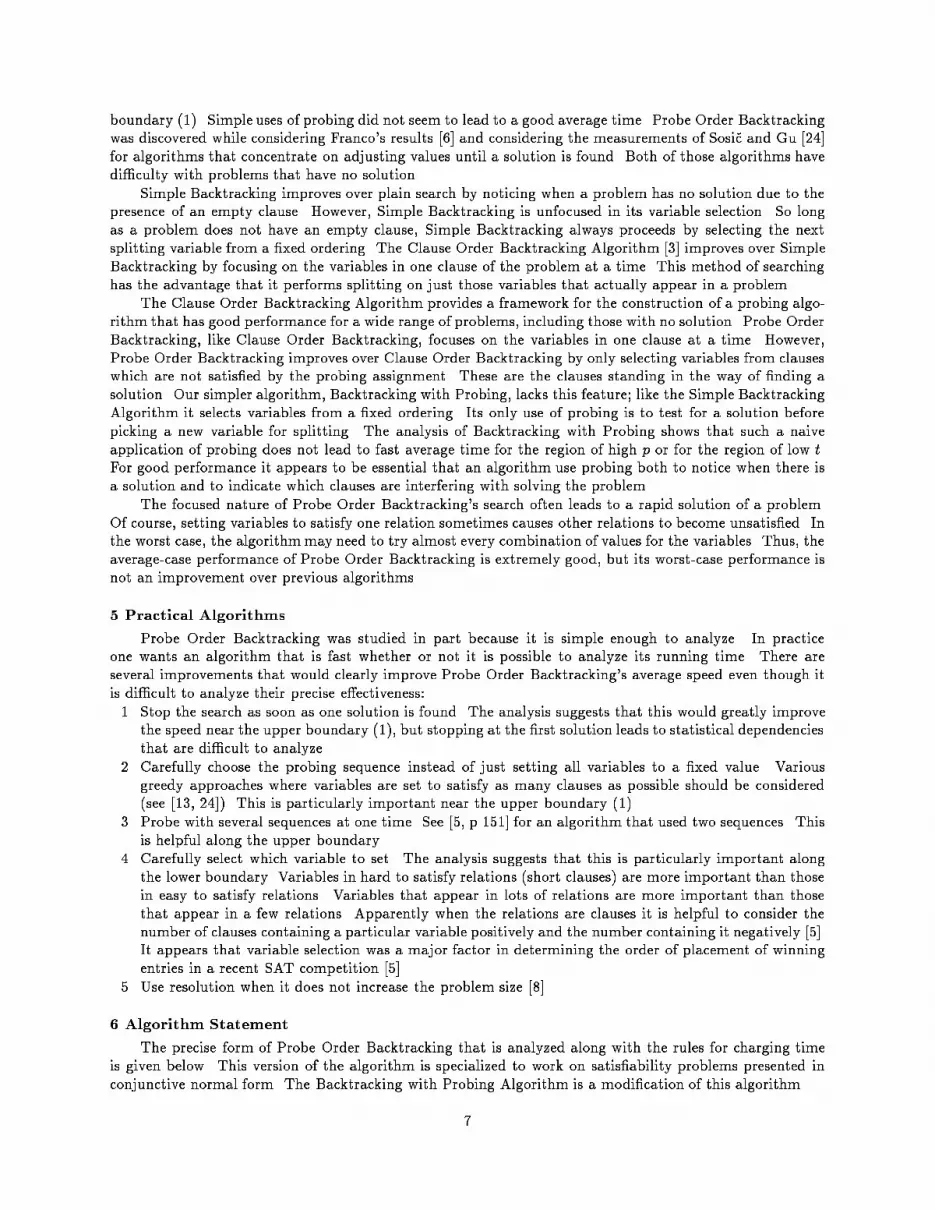
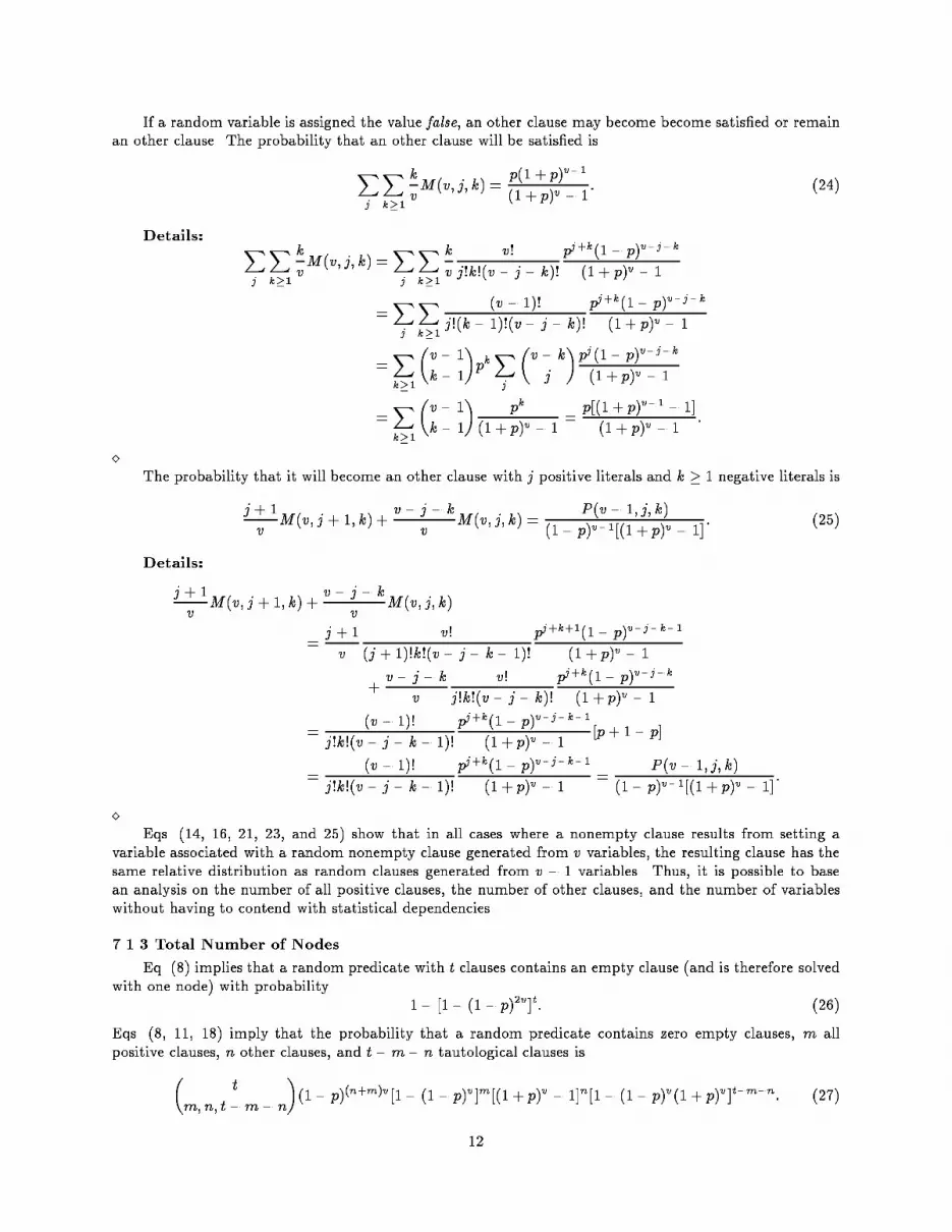
Suppose clauses are generated at random until an other clause is produced. The probability that theother clause contains j positive literals and k � 1 negative literals isM (v; j; k) = P (v; j; k)PjPk�1P (v; j; k) = � vj; k; v� j � k�pj+k(1� p)v�j�k(1 + p)v � 1 : (19)If a random variable is assigned the value true, an other clause may become empty, become all positive,become satis�ed, or remain an other clause. The probability that an other clause will become an emptyclause is 1vM (v; 0; 1) = p(1� p)v�1(1 + p)v � 1 : (20)The probability that it will become an all positive clause with length j is1vM (v; j; 1) = �v � 1j �pj+1(1� p)v�j�1(1 + p)v � 1 = pP (v � 1; j; 0)(1� p)v�1[(1 + p)v � 1] : (21)The probability that it will be satis�ed isXj Xk�1 jvM (v; j; k) = p[(1 + p)v�1 � 1](1 + p)v � 1 (22):Details: Xj Xk�1 jvM (v; j; k) =Xj Xk�1 jv v!j!k!(v � j � k)! pj+k(1� p)v�j�k(1 + p)v � 1=Xj Xk�1 (v � 1)!(j � 1)!k!(v � j � k)! pj+k(1� p)v�j�k(1 + p)v � 1=Xk�1�v � 1k �pkXj �v � 1� kj � 1 �pj(1� p)v�j�k(1 + p)v � 1=Xk�1�v � 1k � pk+1(1 + p)v � 1 = p[(1 + p)v�1 � 1](1 + p)v � 1 :� The probability that it will become an other clause with j positive literals and k � 1 negative literals isk + 1v M (v; j; k + 1) + v � j � kv M (v; j; k) = P (v � 1; j; k)(1� p)v�1[(1 + p)v � 1] : (23)Details:k + 1v M (v; j; k + 1) + v � j � kv M (v; j; k)= k + 1v v!j!(k + 1)!(v � j � k � 1)! pj+k+1(1� p)v�j�k�1(1 + p)v � 1+ v � j � kv v!j!k!(v � j � k)! pj+k(1 � p)v�j�k(1 + p)v � 1= (v � 1)!j!k!(v � j � k � 1)! pj+k(1� p)v�j�k�1(1 + p)v � 1 [p+ 1� p]= (v � 1)!j!k!(v � j � k � 1)! pj+k(1� p)v�j�k�1(1 + p)v � 1 = P (v � 1; j; k)(1� p)v�1[(1 + p)v � 1] :� 11

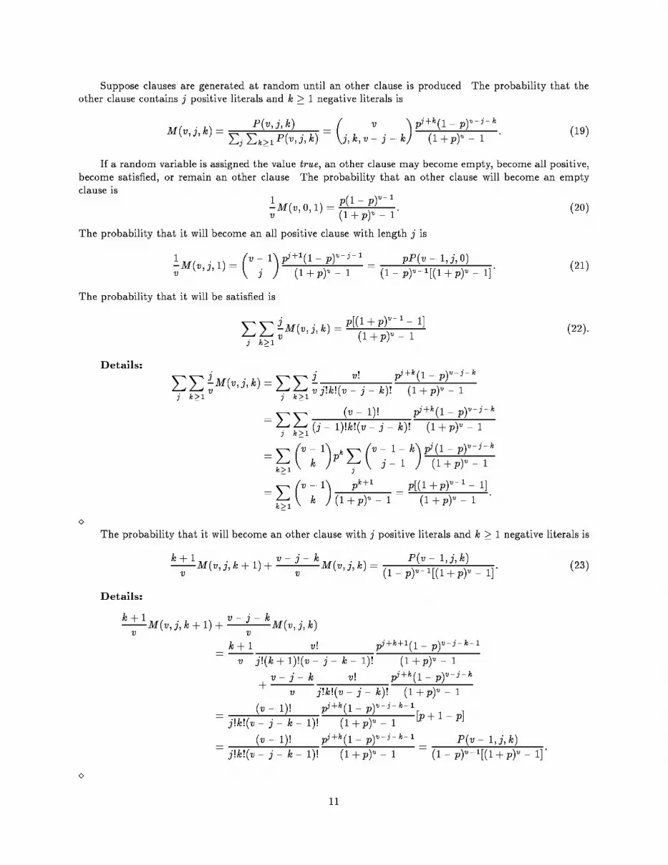
If a random variable is assigned the value false, an other clause may become become satis�ed or remainan other clause. The probability that an other clause will be satis�ed isXj Xk�1 kvM (v; j; k) = p(1 + p)v�1(1 + p)v � 1 : (24)Details: Xj Xk�1 kvM (v; j; k) =Xj Xk�1 kv v!j!k!(v � j � k)! pj+k(1� p)v�j�k(1 + p)v � 1=Xj Xk�1 (v � 1)!j!(k � 1)!(v � j � k)! pj+k(1� p)v�j�k(1 + p)v � 1=Xk�1�v � 1k � 1�pkXj �v � kj �pj(1� p)v�j�k(1 + p)v � 1=Xk�1�v � 1k � 1� pk(1 + p)v � 1 = p[(1 + p)v�1 � 1](1 + p)v � 1 :� The probability that it will become an other clause with j positive literals and k � 1 negative literals isj + 1v M (v; j + 1; k) + v � j � kv M (v; j; k) = P (v � 1; j; k)(1� p)v�1[(1 + p)v � 1] : (25)Details:j + 1v M (v; j + 1; k) + v � j � kv M (v; j; k)= j + 1v v!(j + 1)!k!(v � j � k � 1)! pj+k+1(1� p)v�j�k�1(1 + p)v � 1+ v � j � kv v!j!k!(v � j � k)! pj+k(1� p)v�j�k(1 + p)v � 1= (v � 1)!j!k!(v � j � k � 1)! pj+k(1 � p)v�j�k�1(1 + p)v � 1 [p+ 1� p]= (v � 1)!j!k!(v � j � k � 1)! pj+k(1 � p)v�j�k�1(1 + p)v � 1 = P (v � 1; j; k)(1� p)v�1[(1 + p)v � 1] :� Eqs. (14, 16, 21, 23, and 25) show that in all cases where a nonempty clause results from setting avariable associated with a random nonempty clause generated from v variables, the resulting clause has thesame relative distribution as random clauses generated from v � 1 variables. Thus, it is possible to basean analysis on the number of all positive clauses, the number of other clauses, and the number of variableswithout having to contend with statistical dependencies.7.1.3 Total Number of NodesEq. (8) implies that a random predicate with t clauses contains an empty clause (and is therefore solvedwith one node) with probability 1� [1� (1� p)2v]t: (26)Eqs. (8, 11, 18) imply that the probability that a random predicate contains zero empty clauses, m allpositive clauses, n other clauses, and t �m � n tautological clauses is� tm; n; t�m � n�(1� p)(n+m)v[1� (1� p)v]m[(1 + p)v � 1]n[1� (1� p)v(1 + p)v]t�m�n: (27)12

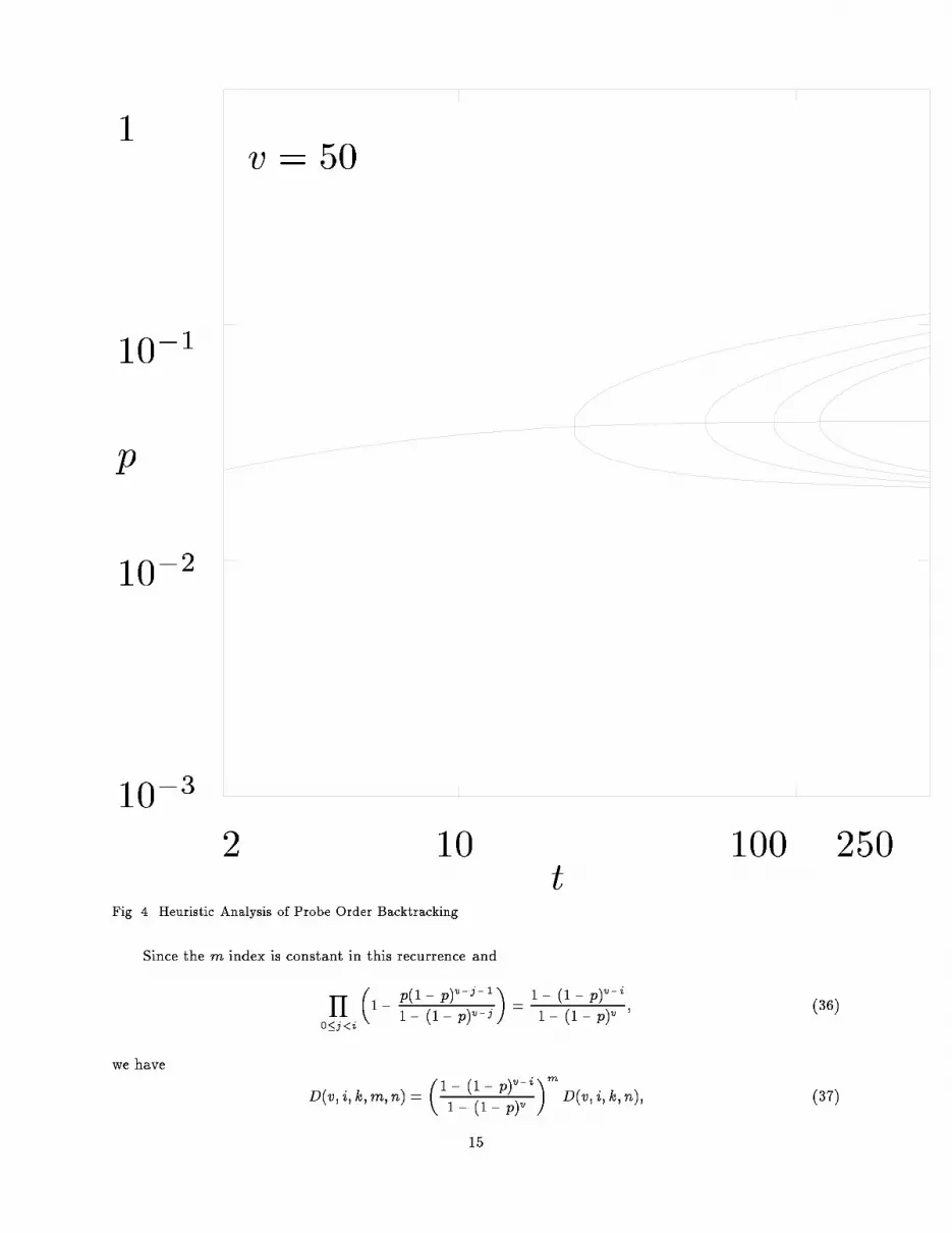
Details: The probability that a clause is empty is (1� p)2v.The probability that a clause is all positive is (1� p)v[1� (1� p)v].The probability that a clause is an other clause is (1� p)v[(1 + p)v � 1].The probability that a clause is none of the above, and hence tautological, is1� (1� p)2v � (1� p)v[1� (1� p)v]� (1 � p)v[(1 + p)v � 1] = 1� (1� p)v(1 + p)v:� If we let T (v;m; n) be the average time required to solve a random problem with v variables, m allpositive clauses, n other clauses, and no empty clauses then by summing all of the cases we see that theexpected number of nodes is1� [1� (1 � p)2v]t +Xm;n� tm; n; t�m� n�(1� p)(n+m)v[1� (1� p)v]m[(1 + p)v � 1]n� [1� (1� p)v(1 + p)v]t�m�nT (v;m; n): (28)This formula applies to both Probe Order Backtracking and Backtracking with Probing so long as thecorresponding de�nition for T is used.7.1.4 Heuristic AnalysisBefore continuing with the exact analysis of the two algorithms we will give a brief heuristic analysisfor the average time used by Probe Order Backtracking.Ignore the fact that setting variables has an e�ect on clauses other than the selected clause. In particular,ignore the fact that the nonselected clauses can become empty or satis�ed and ignore the fact that oncethe variables of one clause are set, there could be fewer variables waiting to be set in the remaining clauses.Under this radical assumption, the number of subproblems produced by splitting on the variables of theselected clause is the same as the length of the selected clause. Eq. (17) implies T (v;m; n) is given by2�� pv1� (1� p)v�m+1 � 1�,�� pv1� (1� p)v�� 1�� 1: (29)Details: If each of m clauses contains w variables, the total number of non-root nodes in the impliedsearch tree satis�es the recurrence N (m) = wN (m� 1) + 2w:`2w' is the number of nodes arising from setting each variable in the clause true and false as speci�ed in theProbe Order Backtracking Algorithm. There are w subproblems produced by splitting. Each subproblemhas m � 1 clauses.The solution to this recurrence is 2 �wm+1 � 1w � 1 �� 2:Add 1 for the root node and use eq. (17) for w to obtain eq. (29).�Plugging into eq. (28) and summing over m and n gives an average number of nodes of1 +� 2pvpv � 1 + (1� p)v�f[1 + (pv � 1)(1� p)v]t � [1� (1� p)2v]tg: (30)Details: De�ne w = pv1� (1� p)v :13

Then1� [1� (1� p)2v]t +Xm;n� tm; n; t�m� n�(1� p)(n+m)v[1� (1� p)v]m[(1 + p)v � 1]n� [1� (1� p)v(1 + p)v]t�m�n�2 �wm+1 � 1w � 1 �� 1�= 1� 2[1� (1� p)2v]t + � 2w � 1�Xm � tm�(1� p)mv [1� (1� p)v]m[1� (1� p)v]t�m �wm+1 � 1= 1�� 2ww � 1� [1� (1� p)2v]t + � 2ww � 1�Xm � tm�[pv(1� p)v]m[1� (1� p)v]t�m= 1�� 2ww � 1� [1� (1� p)2v]t + � 2ww � 1� [1 + (pv � 1)(1� p)v]t= 1�� 2pvpv � 1 + (1� p)v� [1� (1 � p)2v]t +� 2pvpv � 1 + (1� p)v� [1 + (pv � 1)(1� p)v]t:� The contours for this function are given in Fig. 4. Carefully comparing with the true answer (Fig. 2)we see that the heuristic analysis gives neither an upper bound nor a lower bound. For high p the values aretoo small (because changes in clause types were neglected) and for low p the values are too low (because thefact that nonselected clauses can become empty was neglected). This type of analysis can be useful duringinitial algorithm design because it is simple to do, and it often gives roughly the right answer. One mustbeware, however, that on some problems a similar approach might give a radically wrong answer.7.1.5 Transition ProbabilitiesSuppose a predicate is produced by repeatedly generating random clauses from v variables. Supposethe resulting predicate contains m all positive clauses, n other clauses, and no empty clauses.Let G(v; n) be the probability that setting a random variable to true results in the predicate havingone or more empty clauses. When a variable is set to true, other clauses become empty with the probabilitygiven in eq. (20) while all positive clauses do not become empty. Therefore,G(v; n) = 1� �1� p(1� p)v�1(1 + p)v � 1�n : (31)Let F (v;m) be the probability that setting a random variable to false results in a predicate with one ormore empty clauses. Eq. (15) impliesF (v;m) = 1� �1� p(1� p)v�11� (1� p)v�m : (32)Let D(v; i; k;m; n) be the probability that setting i random variables to false results in no clausesbecoming empty and k other clauses becoming satis�ed. If i = 0, nothing happens, soD(v; 0; k;m; n) = �k0: (33)For i = 1, eqs. (15, 24) implyD(v; 1; k;m; n) = �nk��1� p(1� p)v�11� (1� p)v�m � p(1 + p)v�1(1 + p)v � 1�k�1� p(1 + p)v�1(1 + p)v � 1�n�k : (34)For i > 1, some other clauses (x) must be satis�ed when the �rst i � 1 variables are set and then the rest(k � x) must be satis�ed when the last variable is set, so D can be calculated fromD(v; i; k;m; n) =Xx D(v; i � 1; x;m; n)D(v � i + 1; 1; k� x;m; n� x): (35)14

p110�110�210�3

v = 50

2 10 100 250tFig. 4. Heuristic Analysis of Probe Order Backtracking.Since the m index is constant in this recurrence andY0�j<i�1� p(1� p)v�j�11� (1� p)v�j� = 1� (1� p)v�i1� (1� p)v ; (36)we have D(v; i; k;m; n) = �1� (1� p)v�i1� (1� p)v �mD(v; i; k; n); (37)15

where D(v; 1; k; n) = �nk�� p(1 + p)v�1(1 + p)v � 1�k�1� p(1 + p)v�1(1 + p)v � 1�n�k ; (38)and D(v; i; k; n) =Xx D(v; i � 1; x; n)D(v� i + 1; 1; k� x; n� x): (39)By examining small cases, one �ndsD(v; i; k; n) = �nk� [(1 + p)v � (1 + p)v�i]k[(1 + p)v�i � 1]n�k[(1 + p)v � 1]n ; (40)which can be proved by induction.Details: For i = 1 eq. (40) readsD(v; 1; k; n) = �nk� [(1 + p)v � (1 + p)v�1]k[(1 + p)v�1 � 1]n�k[(1 + p)v � 1]n ;which simpli�es to eq. (38). Suppose eq. (39) is true for i = 1 and for i = i� � 1. Then eq. (39) readsD(v; i� ; k; n) =Xx �nx� [(1 + p)v � (1 + p)v�i�+1]x[(1 + p)v�i�+1 � 1]n�x[(1 + p)v � 1]n� �n� xk � x�� p(1 + p)v�i�(1 + p)v�i�+1 � 1�k�x�1� p(1 + p)v�i�(1 + p)v�i�+1 � 1�n�k= �nk�[(1 + p)v�i� � 1]n�k[(1 + p)v � 1]�n�Xx �kx�[(1 + p)v � (1 + p)v�i�+1]x[p(1 + p)v�i� ]k�x;which simpli�es to eq. (40). �Let E(v; j; k; l;m; n) be the probability that setting one random variable to true results in no clausesbecoming empty, j other clauses becoming all positive clauses, k other clauses becoming satis�ed, and l allpositive clauses becoming satis�ed. (Notice that no other changes of clause category can occur.) Eqs. (13,20, 21, 22) implyE(v; j; k; l;m; n) = �ml �� nj; k; n� j � k�� p1� (1� p)v�l�1� p1� (1� p)v�m�l �p[1� (1� p)v�1](1 + p)v � 1 �j� �p[(1 + p)v�1 � 1](1 + p)v � 1 �k �1� p(1 + p)v�1(1 + p)v � 1�n�j�k : (41)Details: From eq. (21) the probability that an other clause will become all positive isXj�1�v � 1j �pj+1(1� p)v�j�1(1 + p)v � 1 = p[1� (1� p)v�1](1 + p)v � 1 :E(v; j; k; l;m; n) = �ml �� nj; k; n� j � k�� p1� (1� p)v�l�1� p1� (1� p)v�m�l �p[1� (1� p)v�1](1 + p)v � 1 �j� �p[(1 + p)v�1 � 1](1 + p)v � 1 �k� �1� p(1� p)v�1(1 + p)v � 1 � p[1� (1� p)v�1](1 + p)v � 1 � p[(1 + p)v�1 � 1](1 + p)v � 1 �n�j�k= �ml �� nj; k; n� j � k�� p1� (1� p)v�l�1� p1� (1� p)v�m�l �p[1� (1� p)v�1](1 + p)v � 1 �j� �p[(1 + p)v�1 � 1](1 + p)v � 1 �k �1� p(1 + p)v�1(1 + p)v � 1�n�j�k :� 16

7.2 Backtracking with ProbingLet T (v;m; n) be the average number of nodes for a problem solved by the Backtracking with ProbingAlgorithm that has v variables, m all positive clauses, and n other clauses, and no empty clauses. If m or nis zero, then the algorithm stops immediately, so there is only one node. Thus,T (v; 0; n) = T (v;m; 0) = 1: (42)If both m and n are bigger than zero, then there are some nodes for the subtree that results when theselected variable is set to false, some nodes for the subtree that results when the selected variable is set totrue, and one node for the root of the search tree.When the variable is set to false, with probability F (v;m) an empty clause is produced (and thereforethere is one node in the subtree). With probability D(v; 1; k;m; n), no empty clauses are produced and k ofthe other clauses become satis�ed, resulting in T (v � 1;m; n� k) as the expected number of nodes in thesubtree.When the variable is set to true, with probability G(v; n) an empty clause is produced. With probabilityE(v; j; k; l;m; n), no empty clauses are produced, j other clauses are converted into all positive clauses, kother clauses are satis�ed, and l all positive clauses are satis�ed, resulting in T (v � 1;m + j � l; n� k � j)as the expected number of nodes in the subtree.For Backtracking with Probing, adding up the nodes from all the cases givesT (v;m; n) = 1 + F (v;m) + G(v; n) +Xk D(v; 1; k;m; n)T (v � 1;m; n� k)+Xj;k;lE(v; j; k; l;m; n)T (v � 1;m+ j � l; n� k � j): (43)7.3 Probe Order BacktrackingProbe Order Backtracking selects a clause and then sets the variables that occur in the clause. If theselected clause has h variables, then there is a root, a node from setting the �rst variable to false, a potentialnode from setting the �rst two variables to false, and so on. This gives a root plus up to h additional nodes.In addition, there is a subtree for setting the �rst variable to true, potentially a subtree for setting the �rstvariable to false and the second to true, and so on. When setting the �rst few variables, some of the otherclauses may evaluate to false. Also, setting the �rst few variables may result in the number of other clausesdropping to zero. Either of these e�ects may prevent a potential node from occurring in the tree.De�ne a(v; i) as the probability that the selected clause contains i or more nodes (thus potentiallycontributing an ith node to the backtrack tree). Then, from eq. (12) we obtaina(v; i) =Xj�i A(v; j) =Xj�i �vj�pj(1� p)v�j1� (1� p)v : (44)Let T (v;m; n) be the average number of nodes for a problem that has v variables, m all positive clauses,n other clauses and no empty clauses. For Probe Order BacktrackingT (v;m; n) = 1 + X1�i�v a(v; i)Xx<nD(v; i � 1; x;m� 1; n)�1 + G(v � i + 1; n� x)+Xj;k;lE(v � i + 1; j; k; l;m� 1; n� x)T (v � i;m+ j � l � 1; n� j � k � x)�: (45)The initial 1 is for the root of the tree. The i index is for those nodes that occur as a result of setting the�rst i variables from the clause. The factor a(v; i) gives the probability that the selected clause has at leasti variables. The index x is for the number of other clauses that are satis�ed when setting the �rst i � 1variables false. The sum does not include x = n, because no subproblems are generated when the number17

of other clauses is reduced to zero. The factor D(v; i� 1; x;m� 1; n) is the probability that x of the n otherclauses become satis�ed and no clauses become empty as a result of setting the �rst i � 1 variables. TheD factor multiplies the sum of terms that relate to the various kinds of nodes that can result when the ithvariable is set. The 1 following the square bracket is for the node that results from setting the ith variableto false. The G(v � i+ 1; n� x) term gives the probability that setting the ith variable to true produces anempty clause. When setting the ith variable to true, the j index counts the number of other clauses thatbecome all positive, the k index counts the number of other clauses that become satis�ed, and the l indexcounts the number of all positive clauses that are satis�ed (the selected clause is not included in this count).The factor E(v� i+1; j; k; l;m�1; n�x) is the probability that setting the ith variable results in the valuesj, k, and l. The factor T (v � i;m+ j � l � 1; n� j � k � x) is the expected number of nodes in the subtreethat results from setting the �rst i� 1 variables to false and the ith variable to true.As with the previous analysis, the boundary conditions are.T (v; 0; n) = T (v;m; 0) = 1: (46)After a number of algebraic transformations eq. (45) can be rewritten asT (v;m; n) = 1 + X1�i�va(v; i)�Z(v; i;m; n) +Xj;k H(v; i; j; k;m; n)T (v � i; j; k)�; (47)where Z(v; i;m; n) = �1� (1� p)v�i+11� (1 � p)v �m�1� �2� �(1 + p)v � (1 + p)v�i+1(1 + p)v � 1 �n �� (1 + p)v � 1� p(1� p)v�i(1 + p)v � 1 �n� ; (48)andH(v; i; j; k;m; n) = �(1 + p)v�i � 1(1 + p)v � 1 �kXl �m � 1l �� nl + j �m + 1��n+m � l � j � 1k ��� p1� (1 � p)v�l �1� (1� p)v�i+1 � p1� (1� p)v �m�l�1 �p[1� (1� p)v�i](1 + p)v � 1 �l+j�m+1�� (1 + p)v � (1 + p)v�i � p(1 + p)v � 1 �n+m�l�j�k�1� �k0�(1 + p)v � (1 + p)v�i+1(1 + p)v � 1 �n��m � 1j ��1� (1 � p)v�i+1 � p1� (1� p)v �j � p1� (1� p)v�m�1�j : (49)Details: De�ne Y (v; i) = 1� (1� p)v�i1� (1 � p)v :Then eqs. (37, 45) implyT (v;m; n) = 1 + X1�i�v a(v; i)Xx<n[Y (v; i � 1)]m�1D(v; i � 1; x; n)�1 +G(v � i+ 1; 1; n� x)+Xj Xk Xl E(v � i+ 1; j; k; l;m� 1; n� x)T (v � i;m + j � l � 1; n� j � k � x)�:� 18

The key idea in the derivation is to �rst change indices with j0 = m + j � l � 1 and k0 = n� j � k � x.Details: Thus, j = l + j0 �m+ 1, k = n+m � l � x� j0 � k0 � 1, andT (v;m; n) = 1 + X1�i�v a(v; i)Xx<n[Y (v; i� 1)]m�1D(v; i � 1; x; n)�1 + G(v � i+ 1; 1; n� x)+Xj Xk XlE(v � i+ 1; l + j �m + 1; n+m � l � x� j � k � 1; l;m� 1; n� x)T (v � i; j; k)�:� Then one computes the sum over x and names the coe�cients to obtain eq. (47).Details: De�neZ(v; i;m; n) = Xx<n[Y (v; i � 1)]m�1D(v; i � 1; x; n)[1+G(v � i + 1; 1; n� x)]:Z(v; i;m; n) = [Y (v; i� 1)]m�1Xx �nx� [(1 + p)v � (1 + p)v�i+1]x[(1 + p)v�i+1 � 1]n�x[(1 + p)v � 1]n (1� �xn)� "2� �1� p(1� p)v�i(1 + p)v�i+1 � 1�n�x#= [Y (v; i� 1)]m�1 �2� �(1 + p)v � (1 + p)v�i+1(1 + p)v � 1 �n �� (1 + p)v � 1� p(1� p)v�i(1 + p)v � 1 �n� :De�ne H(v; i; j; k;m; n) = Xx<n[Y (v; i � 1)]m�1D(v; i � 1; x; n)Xl E(v � i+ 1; l+ j �m + 1; n+m � l � x� j � k � 1; l;m� 1; n� x)= [Y (v; i� 1)]m�1Xx �nx� [(1 + p)v � (1 + p)v�i+1]x[(1 + p)v�i+1 � 1]n�x[(1 + p)v � 1]n (1� �xn)Xl �m� 1l �� n� xl + j �m + 1; n+m � l � x� j � k � 1; k�� p1� (1� p)v�i+1�l� �1� p1� (1� p)v�i+1�m�l�1�p[1� (1� p)v�i](1 + p)v�i+1 � 1�l+j�m+1� �p[(1 + p)v�i � 1](1 + p)v�i+1 � 1�n+m�l�x�j�k�1�1� p(1 + p)v�i(1 + p)v�i+1 � 1�k ;19

H(v; i; j; k;m; n) = [Y (v; i � 1)]m�1Xx [(1 + p)v � (1 + p)v�i+1]x[(1 + p)v�i+1 � 1]n�x[(1 + p)v � 1]n (1� �xn)Xl �m � 1l �� nl + j �m + 1��n +m � l � j � 1k ��n+m � l � j � k � 1x ��� p1� (1� p)v�i+1�l�1� p1� (1� p)v�i+1�m�l�1��p[1� (1 � p)v�i](1 + p)v�i+1 � 1�l+j�m+1 �p[(1 + p)v�i � 1](1 + p)v�i+1 � 1�n+m�l�x�j�k�1��1� p(1 + p)v�i(1 + p)v�i+1 � 1�k= [Y (v; i � 1)]m�1�(1 + p)v�i+1 � 1(1 + p)v � 1 �nXl �m � 1l �� nl + j �m + 1��n +m � l � j � 1k �� p1� (1� p)v�i+1�l��1� p1� (1� p)v�i+1�m�l�1 �p[1� (1� p)v�i](1 + p)v�i+1 � 1�l+j�m+1 �1� p(1 + p)v�i(1 + p)v�i+1 � 1�k�Xx �n +m � l � j � k � 1x �� (1 + p)v � (1 + p)v�i+1(1 + p)v�i+1 � 1 �x��p[(1 + p)v�i � 1](1 + p)v�i+1 � 1�n+m�l�x�j�k�1 (1� �xn)= [Y (v; i � 1)]m�1�(1 + p)v�i+1 � 1(1 + p)v � 1 �nXl �m � 1l �� nl + j �m + 1��n +m � l � j � 1k �� p1� (1� p)v�i+1�l��1� p1� (1� p)v�i+1�m�l�1 �p[1� (1� p)v�i](1 + p)v�i+1 � 1�l+j�m+1 � (1 + p)v�i � 1(1 + p)v�i+1 � 1�k� ��(1 + p)v � (1 + p)v�i � p(1 + p)v�i+1 � 1 �n+m�l�j�k�1� �n+m� l � j � k � 1n �� (1 + p)v � (1 + p)v�i+1(1 + p)v�i+1 � 1 �n�p[(1 + p)v�i � 1](1 + p)v�i+1 � 1�m�l�j�k�1�:Cancel factors to obtain eq. (49).�7.4 Alternate RecurrenceTime O(v2t4) is needed to calculate the average number of nodes for Probe Order Backtracking fromeqs. (28, 47). The following equations calculate the same results in time O(vt4 + v2t3).T (v;m; n; i) = 2[1� (1� p)i](1� p)v�i[(1� p)v � (1� p)2v]m�1[(1� p2)v � (1� p)v]n+ [1� (1� p)i](1� p)v�i(1� p)n+m�1(1� p)v�1Xk �nk�pn�k�Xj J(v � 1;m� 1; n� k; j)T (v � 1; j; k; v� 1)+ p(1� p)n+m�1 X0<f<iXk �nk�[p(1� p2)v�1]kT (v � 1;m; n� k; f); (50)20

T (0;m; n; i) = T (v; 0; n; i) = T (v;m; 0; i) = T (v;m; n; 0) = 0: (51)The factor J(v;m; k; j) may be calculated from the recurrenceJ(v;m; k; j) = [(1� p2)v � (1� p)v]J(v;m; k � 1; j) + J(v;m; k � 1; j � 1)J(v;m; 0; j) = �mj �(1� p)j[p(1� p)v]m�jJ(v;m; k; 0) = [p(1� p)v]m[(1� p2)v � (1� p)v]k: (52)The expected number of nodes for a problem with v variables and t clauses solved by Probe Order Back-tracking is 1 +Xm Xn � tm; n; t�m � n�(1� p)v[1� (1 � p2)v]t�m�nT (v;m; n; v): (53)In order to connect this version of the analysis to the analysis expressed in eqs. (28, 47) we de�ne�(v;m; n; i) = [1� (1� p)i](1� p)v�i[(1� p)v � (1� p)2v]m�1[(1� p2)v � (1� p)v]n: (54)Then we may relate T from eq. (50) to T from eq. (47) viaT (v;m; n; v) = �(v;m; n; v)[T (v;m; n)� 1]: (55)T (v;m; n; i)=�(v;m; n; i) is the expected number of non-root nodes in the backtrack tree generated bya problem with v variables, n other clauses, m all positive clauses, and no empty clauses such that the �rstall positive clause may not contain any of the �rst v� i variables. The �rst three parameters have the samemeaning as the corresponding parameters from eq. (47). The fourth parameter, i, keeps track of the e�ectsetting literals false has in shortening the �rst all positive clause during the course of the algorithm. Thefactor �(v;m; n; i) is chosen so that no divisions are needed to evaluate eqs. (50{53).Although eq. (50) uses four indices, it is a full-history recurrence in only three indices: m, n, and i.Hence T (v;m; n; i) may be calculated in space O(vt2).Details: Eqs. (50{53) are an analysis of the same algorithm as eqs. (28, 47). However, in derivingeqs. (50{53) it is clearest to restate the Probe Order Algorithm in an equivalent but more explicitly recursiveform. Begin by establishing a canonical ordering of the literals and clauses in the predicate. Remove alltautological clauses. Then:1. (Test: Empty Predicate) If the predicate is empty, return the solution.2. (Test: Empty Clause) If any clause is empty, return with no solution.3. (Probe: Negatively-Augmented Solution) If all remaining clauses have a negative literal, returnthe negatively-augmented solution. (That is, check for m = 0.)4. (Partial Probe: Positively-Augmented Solution) If no remaining clauses have a negative literal,return the positively-augmented solution. (That is, check for n = 0.)5. (Splitting: Clause-Order Recursion) Consider the �rst positive literal (according to the canonicalordering of the literals) appearing in the �rst all positive clause:a. (Assert the Literal.) Set the literal true. Simplify the predicate. Charge one time unit. Recurwith the simpli�ed predicate.b. (Negate the Literal.) Set the literal false. Simplify the predicate. Charge one time unit. Recurwith the simpli�ed predicate.Conclude the algorithm by charging one time unit for the root.We count the nodes in the backtrack tree by recursively counting the nodes introduced by each step ofthe algorithm. We must keep track of how many all positive clauses and how many other clauses remain ateach stage of the algorithm. In addition we must keep track of events that a�ect the length of the �rst allpositive clause.Let T1(v;m; n; i) be the expected number of nodes (exclusive of the root) in the backtrack tree generatedby a call to Probe Order Backtracking on a predicate with v variables, m all positive clauses, n other21

clauses, and no empty clauses, in which the �rst all positive clause is drawn from the last i variables inthe canonical listing of variables. We shall see that T1(v;m; n; i) is related to T (v;m; n; i) from eq. (50) viaT (v;m; n; i) = �(v;m; n; i)T1(v;m; n; i).Let Q(t; v) be the expected number of nodes in the backtrack tree generated by a call to Probe OrderBacktracking on a predicate with t clauses and v variables. Then from eq. (28) we haveQ(t; v) = 1 +Xm Xn � tm; n; t�m� n�[(1� p)v � (1� p)2v]m� [(1� p2)v � (1� p)v]n[1� (1� p2)v]t�m�nT1(v;m; n; v):In degenerate cases the algorithm does not set any variables. Hence the natural boundary conditionsfor T1(v;m; n; i) are T1(0;m; n; i) = T1(v; 0; n; i) = T1(v;m; 0; i) = T1(v;m; n; 0) = 0:Nodes may be introduced in one of two ways: the algorithmAsserts the Literal, or the algorithmNegatesthe Literal. Let us denote the expected number of nodes introduced by these branches as A(v;m; n; i) andN (v;m; n; i), respectively. WriteT1(v;m; n; i) = A(v;m; n; i) + N (v;m; n; i):We now determine the equations for A(v;m; n; i) and N (v;m; n; i). �Details: 7.4.1 Derivation of ASuppose the �rst literal in the �rst all positive clause is asserted. One time unit is charged and thepredicate is simpli�ed. Probe Order Backtracking is called recursively on the simpli�ed predicate.Using eq. (41), the total number of nodes introduced by setting the literal true is given byA(v;m; n; i) = 1 +Xj Xk Xl E(v; j; k; l;m� 1; n)T1(v � 1;m� 1 + j � l; n� j � k; v � 1):Notice that A(v;m; n; i) is independent of i. It is useful to de�ne A(v;m; n) = A(v;m + 1; n; i) (notice theshift in the m index). �Details: 7.4.2 Derivation of NSuppose the �rst literal in the �rst all positive clause is set false. One time unit is charged and thepredicate is simpli�ed. Probe Order Backtracking is called recursively on the simpli�ed predicate.The �rst all positive clause is drawn from a population of i variables (the last i variables in the canonicallisting of variables). The probability that a random clause drawn from i variables contains no variableappearing negatively is (1 � p)i. The probability that none of the �rst i � f � 1 variables occurs positivelyin the clause is (1 � p)i�f�1. The probability that this clause contains the positive form of the (i � f)thvariable is p. The probability that at least one of the remaining f variables occurs positively is 1� (1� p)f .Eq. (11) gives the probability that a random clause is all positive. Combining all these factors, we obtainthe probability, given a random all-positive clause in i variables, that the �rst literal to appear in this clausewill be the positive form of the (i � f)th variable in the canonical listing of the i variables, and that aftersetting the (i� f)th literal false the clause is not empty:(1 � p)i(1� p)i�f�1p[1� (1� p)f ](1� p)i � (1� p)2i = p(1� p)i�f�1 � p(1� p)i�11� (1� p)i :Stated another way, this is the probability that setting the �rst literal false in the �rst all positive clausewill result in a subproblem in which the �rst all positive clause is drawn from a population of f variables.From eq. (34) and the preceding discussion, setting the literal false leaves a problem in v � 1 variables,m all positive clauses, n � k other clauses, and no empty clauses, in which the �rst all positive clause isdrawn from the last f variables with probability�p(1� p)i�f�1 � p(1� p)i�11� (1 � p)i �D(v; 1; k;m� 1; n):Summing over all cases, the total number of nodes introduced by setting the literal false is given byN (v;m; n; i) = 1 +Xk X0<f<i �p(1� p)i�f�1 � p(1� p)i�11� (1� p)i �D(v; 1; k;m� 1; n)T1(v � 1;m; n� k; f):� 22

Details: 7.4.3 Full Set of Equations for the Alternate RecurrenceWe now simplify the following set of equations:Q(t; v) = 1 + X0<m<t X0<n�t�m� tm; n; t�m� n�[(1� p)v � (1� p)2v]m� [(1� p2)v � (1� p)v]n[1� (1� p2)v]t�m�nT1(v;m; n; v);T1(v;m; n; i) = A(v;m � 1; n) +N (v;m; n; i);T1(0;m; n; i) = T1(v; 0; n; i) = T1(v;m; 0; i) = T1(v;m; n; 0) = 0;A(v;m; n) = 1 +Xj Xk Xl E(v; j; k; l;m; n)T1(v � 1;m+ j � l; n� j � k; v � 1);N (v;m; n; i) = 1 +Xk X0<f<i �p(1� p)i�f�1 � p(1� p)i�11� (1� p)i �D(v; 1; k;m� 1; n)T1(v � 1;m; n� k; f):Perform the index changes j0 = m + j � l and k0 = n � k � j in A(v;m; n).A(v;m; n) = 1 +Xj;k;lE(v; j �m + l; n+m � j � k � l; l;m; n)T1(v � 1; j; k; v� 1):Plug in the de�nition for E from eq. (41).A(v;m; n) = 1 +Xj;k;l�ml �� nj �m+ l; n+m � j � k � l; k�� p1� (1� p)v�l��1� p1� (1� p)v�m�l �p[1� (1� p)v�1](1 + p)v � 1 �j�m+l �p[(1 + p)v�1 � 1](1 + p)v � 1 �n+m�j�k�l��1� p(1 + p)v�1(1 + p)v � 1�k T1(v � 1; j; k; v� 1):Clear some fractions to yield:A(v;m; n) = 1 + � (1� p)v(1� p)v[(1 + p)v � 1]�n � (1� p)v(1 � p)v[1� (1� p)v]�mXj;k;l�ml ��nk�� n� kj � (m � l)�� pl(1 � p)m�lpn�k[1� (1� p)v�1]j[(1 + p)v�1 � 1]n+m�j�lT1(v � 1; j; k; v� 1):In order to guard against oating point over ow due to the factor of (1+p)v�1 we have introduced a factorof (1� p)v(m+n)=(1� p)v(m+n) into the summation. Multiplying this through givesA(v;m; n) = 1 + (1� p)n+m � 1(1� p2)v � (1� p)v �n � 1(1� p)v � (1� p)2v �mXj;k;l�ml ��nk�� n� kj � (m� l)�� pl(1� p)m�lpn�k[(1� p)v�1 � (1� p)2v�2]j[(1� p2)v�1 � (1� p)v�1]k[(1� p)v�1]l� [(1� p2)v�1 � (1� p)v�1]n�k�j+(m�l)T1(v � 1; j; k; v� 1):Collect all the terms that depend on l and de�neJ(v;m; k; j) =Xl �ml �� kj � (m � l)�(1 � p)m�l[p(1� p)v]l[(1� p2)v � (1� p)v]k�j+(m�l);then, after rearranging to emphasize speed of computation, we may writeA(v;m; n) = 1 + (1� p)n+m � 1(1� p2)v � (1� p)v �n � 1(1� p)v � (1� p)2v �m�Xk �nk�pn�k[(1� p2)v�1 � (1� p)v�1]k�Xj [(1� p)v�1 � (1� p)2v�2]jJ(v � 1;m; n� k; j)T1(v � 1; j; k; v� 1):23

We avoid explicitly performing the sum over l in the evaluation of J(v;m; k; j) by using a recurrencefor J(v;m; k; j). Using a recurrence for the binomial coe�cient we haveJ(v;m; k; j) =Xl �ml �� k � 1j � (m � l)�(1 � p)m�l[p(1� p)v]l[(1� p2)v � (1� p)v]k�j+(m�l)+Xl �ml �� k � 1(j � 1)� (m � l)�(1� p)m�l[p(1� p)v]l[(1� p2)v � (1� p)v]k�j+(m�l)= [(1� p2)v � (1� p)v]�Xl �ml �� k � 1j � (m� l)�(1� p)m�l[p(1� p)v]l[(1� p2)v � (1� p)v]k�1�j+(m�l)+Xl �ml �� k � 1(j � 1)� (m � l)�(1� p)m�l[p(1� p)v]l[(1� p2)v � (1� p)v]k�1�(j�1)+(m�l)= [(1� p2)v � (1� p)v]J(v;m; k� 1; j) + J(v;m; k � 1; j � 1):To get the boundary conditions in eq. (52) note that the sum for J(v;m; k; j) can be evaluated directly whenk = 0 or j = 0. J(v;m; 0; j) = �mj �(1� p)j[p(1� p)v]m�jJ(v;m; k; 0) = [p(1� p)v]m[(1� p2)v � (1 � p)v]k:Now we work on N (v;m; n; i). Plug the de�nition for D(v; 1; k;m�1; n) from eq. (34) into N (v;m; n; i).N (v;m; n; i) = 1 +Xk X0<f<i �p(1� p)i�f�1 � p(1� p)i�11� (1� p)i ��nk��1� p(1� p)v�11� (1 � p)v�m�1� � p(1 + p)v�1(1 + p)v � 1�k�1� p(1 + p)v�1(1 + p)v � 1�n�k T1(v � 1;m; n� k; f):Clearing fractions in N (v;m; n; i) gives:N (v;m; n; i) = 1 + p� (1� p)v(1� p)v[(1 + p)v � 1]�n� (1� p)v(1� p)v[1� (1� p)v]�m�1 � (1� p)i�11� (1� p)i ��Xk X0<f<i �1� (1� p)f(1� p)f ��nk�[1� (1� p)v�1]m�1� [p(1 + p)v�1]k[(1 + p)v�1 � 1]n�kT1(v � 1;m; n� k; f):Again, in order to guard against oating point over ow due to the factor of (1 + p)v � 1, we haveintroduced a factor of (1� p)v(m�1+n)=(1 � p)v(m�1+n) into the summation. Multiplying this through andrearranging givesN (v;m; n; i) = 1 + p(1� p)n+m�1 � 1(1� p2)v � (1� p)v �n � 1(1 � p)v � (1� p)2v �m�1 � (1� p)i�11� (1� p)i �� X0<f<iXk �nk�[p(1� p2)v�1]k[(1� p2)v�1 � (1� p)v�1]n�k� [(1� p)v�1 � (1� p)2v�2]m�1 �1� (1� p)f(1� p)f �T1(v � 1;m; n� k; f):24

Now plug the de�nitions for A(v;m � 1; n) and N (v;m; n; i) into T1(v;m; n; i).T1(v;m; n; i) = 2 + (1 � p)n+m�1 � 1(1� p2)v � (1� p)v �n � 1(1� p)v � (1 � p)2v �m�1�Xk �nk�pn�k[(1� p2)v�1 � (1� p)v�1]k�Xj [(1� p)v�1 � (1 � p)2v�2]jJ(v � 1;m� 1; n� k; j)T1(v � 1; j; k; v� 1)+ p(1� p)n+m�1 � 1(1� p2)v � (1� p)v �n � 1(1� p)v � (1� p)2v �m�1 � (1� p)i�11� (1� p)i�� X0<f<iXk �nk�[p(1� p2)v�1]k[(1� p2)v�1 � (1 � p)v�1]n�k� [(1� p)v�1 � (1� p)2v�2]m�1 �1� (1� p)f(1 � p)f �T1(v � 1;m; n� k; f):To clear the rest of the fractions we rede�ne T1(v;m; n; i):T (v;m; n; i) = [1� (1� p)i](1� p)v�i[(1� p)v � (1� p)2v]m�1[(1� p2)v � (1� p)v]nT1(v;m; n; i)= �(v;m; n; i)T1(v;m; n; i):Making this substitution yields equations (50) and (53).�Details: 7.5 Veri�cation of the RecurrencesAside from being careful with the mathematics, we performed measurements to help insure the correct-ness of the analyses of Backtracking with Probing and of Probe Order Backtracking.For each algorithm and for t and v in the range 1 � v � 6, 1 � t � 6, 1 � tv � 12, we generated each ofthe 22tv SAT problems and counted the number of nodes produced. A problem with i literals has probabilitypi(1�p)2tv�i. Multiplying the node counts for each i by the probability gives a polynomial in p with integercoe�cients [3]. We used Maple to solve each recurrence (28, 43, 47, 50, 53) algebraically and veri�ed thatthe polynomials from the recurrences were identical with the polynomials generated from the correspondingnode counts.We veri�ed that the two analyses of the Probe Order Backtracking Algorithm, eqs. (28, 47) andeqs. (50, 53), predicted the same values in two ways. First, we used Maple to solve each recurrence al-gebraically for 1 � t � 6 and 1 � v � 6 and veri�ed that the formulas were identical. Second, we used eachrecurrence to compute contours for v = 50 and t � 179. The locations of the contours were identical towithin the precision to which they were computed. The worst p performance matched to an accuracy of 9digits.�8 BoundsSimple upper bounds on the running time for Probe Order Backtracking are now computed. Theapproach is to eliminate indices from the recurrence until one has a simple algebraic equation. To eliminate anindex, we assume that the unknown function (T ) has a particular dependence on the index being eliminatedtimes a new unknown function of the remaining indices. By plugging the assumed form into the initialrecurrence (and performing one or two summations), we obtain a bounding recurrence for the new function.To simplify the algebra, we now drop the term that starts with �k0 from the de�nition of H [in eq. (49)]and drop the �rst negative term from the de�nition of Z [in eq. (48)]. These changes lead to a new T (v;m; n),which is an upper bound on the running time of the algorithm. They have no signi�cant e�ect on thecomputed running time when v is large. Dropping them now saves a lot of ink.It is convenient to �rst shift the recurrence by using T 0(v;m; n) = T (v;m; n) � 1. From eq. (47) weobtainT 0(v;m; n) = X1�i�v a(v; i)�Z(v; i;m; n) +Xj Xk H(v; i; j; k;m; n)[T 0(v � i; j; k) + 1]�25

= X1�i�v a(v; i)�Z(v; i;m; n) +�1� (1� p)v�i+11� (1� p)v �m�1�(1 + p)v � 1� p(1 + p)v�i(1 + p)v � 1 �n+Xj Xk H(v; i; j; k;m; n)T 0(v � i; j; k)�; (56)which can be written asT 0(v;m; n) = X1�i�va(v; i)�Z0(v; i;m; n) +Xj Xk H(v; i; j; k;m; n)T 0(v � i; j; k)�; (57)where Z 0(v; i;m; n) = 2�1� (1� p)v�i+11� (1� p)v �m�1 : (58)The boundary conditions for the shifted recurrence areT 0(v; 0; n) = T 0(v;m; 0) = 0; (59)and the average number of nodes is1+Xm;n� tm; n; t�m � n�(1� p)(n+m)v[1� (1� p)v]m[(1 + p)v � 1]n[1� (1� p)v(1 + p)v]t�m�nT 0(v;m; n):(60)Details: SummingH over k givesXk H(v; i; j; k;m; n) =Xk � (1 + p)v�i � 1(1 + p)v � 1 �kXl �m � 1l �� nl + j �m + 1��n+m� l � j � 1k ��� p1� (1� p)v�l �1� (1� p)v�i+1 � p1� (1� p)v �m�l�1��p[1� (1� p)v�i](1 + p)v � 1 �l+j�m+1 � (1 + p)v � (1 + p)v�i � p(1 + p)v � 1 �n+m�l�j�k�1=Xl �m � 1l �� nl + j �m + 1�� p1� (1� p)v�l�1� (1� p)v�i+1 � p1� (1� p)v �m�l�1��p[1� (1� p)v�i](1 + p)v � 1 �l+j�m+1 � (1 + p)v � 1� p(1 + p)v � 1 �n+m�l�j�1 :Summing H over k and j givesXj;kH(v; i; j; k;m; n)=Xj Xl �m� 1l �� nl + j �m + 1�� p1� (1� p)v�l �1� (1� p)v�i+1 � p1� (1� p)v �m�l�1��p[1� (1� p)v�i](1 + p)v � 1 �l+j�m+1 �(1 + p)v � 1� p(1 + p)v � 1 �n+m�l�j�1=Xl �m � 1l �� p1� (1� p)v�l �1� (1� p)v�i+1 � p1� (1� p)v �m�l�1�� (1 + p)v � 1� p(1 � p)v�i(1 + p)v � 1 �n= �1� (1 � p)v�i+11� (1� p)v �m�1� (1 + p)v � 1� p(1� p)v�i(1 + p)v � 1 �n :26

Z 0(v; i;m; n) = �1� (1� p)v�i+11� (1 � p)v �m�1 �2� �(1 + p)v � 1� p(1� p)v�i(1 + p)v � 1 �n�+ �1� (1� p)v�i+11� (1� p)v �m�1�(1 + p)v � 1� p(1 + p)v�i(1 + p)v � 1 �n ;which simpli�es to eq. (58). �8.1 Two Index RecurrenceFor any x(v) de�ne T (v; n) so that T 0(v;m; n) � x(v)mT (v; n) for allm. (We could include n dependencein x, but that does not appear to be useful.) Drop the �k0 term from the de�nition ofH (eq. 49) and rearrangethe binomials.Details: To help sum in the j direction, rearrange the binomials in the de�nition of H asH(v; i; j; k;m; n) = �nk�� (1 + p)v�i � 1(1 + p)v � 1 �kXl �m� 1l �� n � kl + j �m+ 1�� p1� (1� p)v�l��1� (1� p)v�i+1 � p1� (1� p)v �m�l�1 �p[1� (1 � p)v�i](1 + p)v � 1 �l+j�m+1�� (1 + p)v � (1 + p)v�i � p(1 + p)v � 1 �n+m�l�j�k�1 :� Combine this H with the de�nition of Z 0 (eq. 58). Use the de�nition of T (v; n) and sum over j to obtainT (v; n) = 1x(v) maxm � X1�i�v a(v; i)�2� 1� (1� p)v�i+1x(v)[1� (1� p)v]�m�1+ �x(v � i)[1� (1� p)v�i+1] + [1� x(v � i)]px(v)[1� (1� p)v] �m�1�Xk �nk�� (1 + p)v�i � 1(1 + p)v � 1 �k� �(1 + p)v � (1 + p)v�i � [1� x(v � i)]p� x(v � i)p(1 � p)v�i(1 + p)v � 1 �n�k T (v � i; k)��:(61)T (v; 0) = 0; T (v; n) � 0: (62)Details: Summing xjH over j gives 27

Xj xjH(v; i; j; k;m; n)=Xj xj��nk��(1 + p)v�i � 1(1 + p)v � 1 �kXl �m � 1l �� n� kl + j �m + 1�� p1� (1� p)v�l��1� (1� p)v�i+1 � p1� (1� p)v �m�l�1�p[1� (1� p)v�i](1 + p)v � 1 �l+j�m+1�� (1 + p)v � (1 + p)v�i � p(1 + p)v � 1 �n+m�l�j�k�1= �nk��(1 + p)v�i � 1(1 + p)v � 1 �k �(1 + p)v � (1 + p)v�i � (1� x)p� xp(1� p)v�i(1 + p)v � 1 �n�k�Xl �m� 1l �� p1� (1� p)v�l xm�l�1�1� (1� p)v�i+1 � p1� (1� p)v �m�l�1= �x[1� (1� p)v�i+1] + (1� x)p1� (1� p)v �m�1��nk�� (1 + p)v�i � 1(1 + p)v � 1 �k� (1 + p)v � (1 + p)v�i � (1� x)p� xp(1� p)v�i(1 + p)v � 1 �n�k :Eq. (57) implies that we needx(v)mT (v; n) � X1�i�v a(v; i)�Z(v; i;m; n) +Xj Xk x(v � i)jH(v; i; j; k;m; n)T (v � i; k)�;T (v; 0) = 0; T (v; n) � 0;where the bounds must hold for all m of interest. Thus,T (v; n) = maxm � 1x(v)m � X1�i�v a(v; i)�Z(v; i;m; n) +Xj Xk x(v � i)jH(v; i; j; k;m; n)T (v � i; k)���;T (v; 0) = 0:Using the sum of xjH and the de�nition of Z, we obtain eq. (61).�So that this recurrence will be favorable, we wish to avoid raising quantities that are above 1 to the mpower. Thus, we require [1� (1� p)v]x(v) � 1� (1� p)v�i+1; (63)and [1� (1� p)v]x(v) � [1� (1� p)v�i+1]x(v � i) + [1� x(v � i)]p: (64)So long as x(v) is above 1, then any increasing function of v can be chosen for [1� (1� p)v]x(v).If x(v) obeys the bounds (63, 64), then we may letT (v; n) = 1x(v)� X1�i�v a(v; i)�2 +Xk �nk�� (1 + p)v�i � 1(1 + p)v � 1 �k� �(1 + p)v � (1 + p)v�i � [1� x(v � i)]p � x(v � i)p(1 � p)v�i(1 + p)v � 1 �n�k T (v � i; k)��: (65)28

Eq. (60) implies the average number of nodes is bounded by1+Xm;n� tm; n; t�m � n�(1� p)(n+m)vx(v)m[1� (1� p)v]m� [(1 + p)v � 1]n[1� (1� p)v(1 + p)v]t�m�nT (v; n)= 1 +Xn � tn�(1� p)nv[(1 + p)v � 1]nf1� (1� p)v(1 + p)v + x(v)(1� p)v[1� (1� p)v]gt�nT (v; n):(66)Eq. (66) gives a good bound when x(v) is set to the average length of an all positive clause, eq. (17).Figure 5 shows the bounds that result from this value of x.Details:Figure 5a shows the bound when x(v) = a(p; t; v)pv1� (1� p)vand a(p; t; v) has the value computed at the end of Section 8.3.�Note the division by x(v) in eq. (65). This is critical to obtaining an analytical understanding of whyProbe Order Backtracking is fast. We are free to set x(v) large enough to cancel out the e�ect of summingover i (which is where the growth in T (v; n) comes from) so long as the factor in eq. (66) which is raisedto the t � n power is not above 1. This division by x(v) is related to the fact that selecting an all positiveclause results in a reduction of one in the number of all positive clauses (the setting of variables can augmentor counteract this reduction). In Backtracking with Probing we do not have this tendency to reduce thenumber of all positive clauses by 1, and thus that algorithm is often much slower.8.2 One Index RecurrenceFor any x(v) and y(v) de�ne T (v) so that T 0(v;m; n) � x(v)my(v)nT (v) for allm and n. Then a suitableT (v) is any function at least as large as the solution toT (v) = 1x(v) maxm;n� X1�i�v a(v; i)� � 2y(v)n � 1� (1� p)v�i+1x(v)[1� (1� p)v]�m�1+ �x(v � i)[1� (1� p)v�i+1] + [1� x(v � i)]px(v)[1� (1� p)v] �m�1�� (1 + p)v + [y(v � i) � 1](1 + p)v�i � y(v � i)� [1� x(v � i)]p� x(v � i)p(1� p)v�iy(v)[(1 + p)v � 1] �n� T (v � i)��: (67)Details: Summing xjykH over j and k givesXj;k xjykH(v; i; j; k;m; n)=Xk yk �x[1� (1� p)v�i+1] + (1� x)p1� (1� p)v �m�1��nk�� (1 + p)v�i � 1(1 + p)v � 1 �k� (1 + p)v � (1 + p)v�i � (1� x)p� xp(1� p)v�i(1 + p)v � 1 �n�k= �x[1� (1� p)v�i+1] + (1� x)p1� (1� p)v �m�1� �(1 + p)v + (y � 1)(1 + p)v�i � y � (1 � x)p� xp(1� p)v�i(1 + p)v � 1 �n :29

p110�110�210�3

v = 50

2 10 100 250tFig. 5. Two index upper limit.Using this sum in eq. (61) gives eq. (67). �Again, we wish to avoid raising quantities above 1 to high powers. Thus, we still have bounds (63, 64)for x(v). In addition we have y(v) � 1; (68)and [y(v) � 1][(1 + p)v � 1]� [y(v � i) � 1][(1 + p)v�i � 1] � pfx(v � i)[1� (1� p)v�i]� 1g: (69)30

p110�110�210�3

v = 50

2 10 100 250tFig. 5a. Two index upper limit, improved x.These bounds for y are satis�ed by[y(v) � 1][(1 + p)v � 1] = p X1�j�v�1maxf0; fx(j)[1� (1� p)j ]� 1gg: (70)If x(v) and y(v) obey the bounds, we haveT (v) = 1x(v) X1�i�va(v; i)[2 + T (v � i)]: (71)31

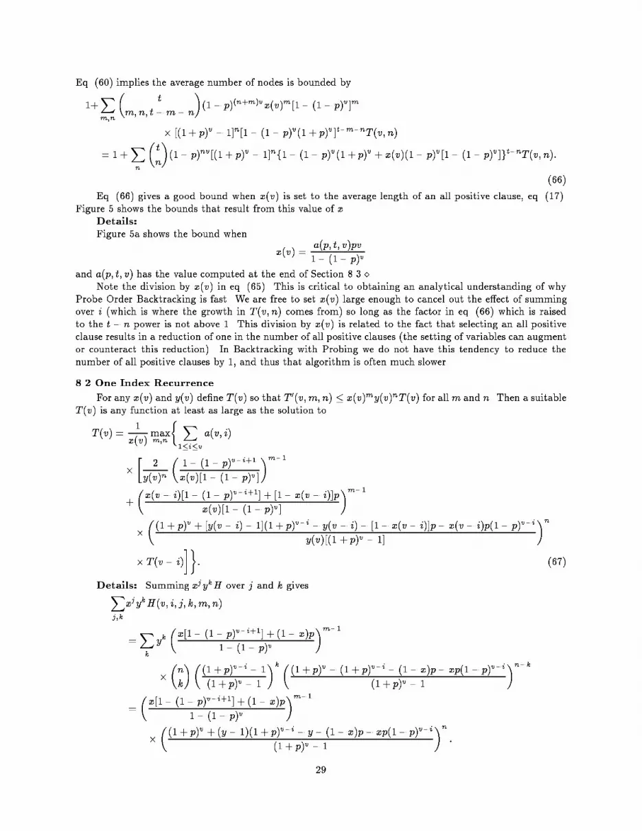
Eq. (66) implies the average number of nodes is bounded by1 +Xn �tn�y(v)n(1� p)nv[(1 + p)v � 1]nf1� (1� p)v(1 + p)v + x(v)(1 � p)v[1� (1� p)v]gt�nT (v)= 1 + f1� (1� p)v(1 + p)v + y(v)(1 � p)v[(1 + p)v � 1] + x(v)(1 � p)v[1� (1� p)v]gtT (v): (72)If the value of y(v) is set by eq. (70), then the number of nodes is bounded by1 + �1 + (1� p)v�x(v)[1� (1� p)v]� 1 + p X1�j�v�1maxf0; (x(j)[1� (1 � p)j ]� 1)g��tT (v): (73)Eq. (73) gives a good bound when x(v) is set to the average length of an all positive clause, eq. (17).Figure 6 shows the bounds that result from this value of x.Details:Figure 6a shows the bound when x is given an improved value that is discussed in Section 8.3. �If one ignores the requirement that y(v) satisfy bounds (68, 69) and just sets x(v) to the average clausesize and y(v) = 1, one obtains a result that is essentially the same as that given by the heuristic analysis,eq. (30).8.3 Zero IndicesEq. (71) has only one index, but it is still rather complex due to the summation on the right side.Therefore, we will again eliminate an index from the recurrence.Assume T (v) is no more than T for v < v�. (This assumption does not lead to much error when T issmall; if one wishes a good approximation when T is large, one should consider T (v) � Tzv and select thebest value for z.) We obtain T (v�) � 2 + Tx(v) X1�i�v a(v; i): (74)A good choice for x(v) is one that cancels the e�ect of the summation. Forx(v) = pv1� (1� p)v ; (75)we have X1�j�v�1maxfx(j)[1� (1� p)j ]� 1; 0g = X1=p�j�v�1(pj � 1)� pv(v � 1)2 � (1=p� 1)2 ��v � 1p� ; (76)(the less than or equal comes from the fact that 1=p may be a noninteger). Thus, eqs. (73, 76) imply thatthe number of nodes is bounded by T (v�) = 2 + T; (77)which is satis�ed for all v if we take T (v) = 2v: (78)Details: From the de�nition of a(v; i), eq. (44),Xi�1 a(v; i) = Xi�1 Xj�i�vj�pj(1� p)v�j1� (1 � p)v =Xj�1 X1�i�j�vj�pj(1� p)v�j1 � (1� p)v= vXj�1�v � 1j � 1�pj(1� p)v�j1� (1� p)v = pv1� (1� p)v :� 32

p110�110�210�3

v = 50

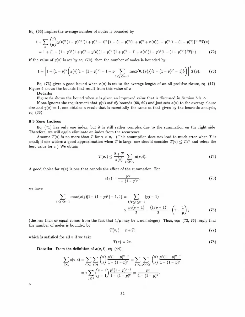
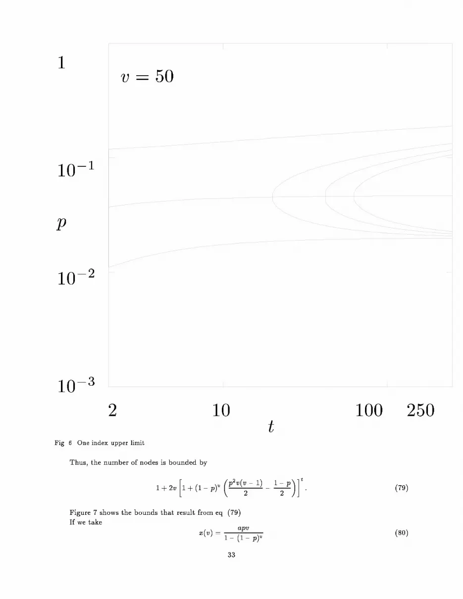
2 10 100 250tFig. 6. One index upper limit.Thus, the number of nodes is bounded by1 + 2v �1 + (1� p)v �p2v(v � 1)2 � 1� p2 ��t : (79)Figure 7 shows the bounds that result from eq. (79).If we take x(v) = apv1� (1� p)v (80)33

p110�110�210�3

v = 50

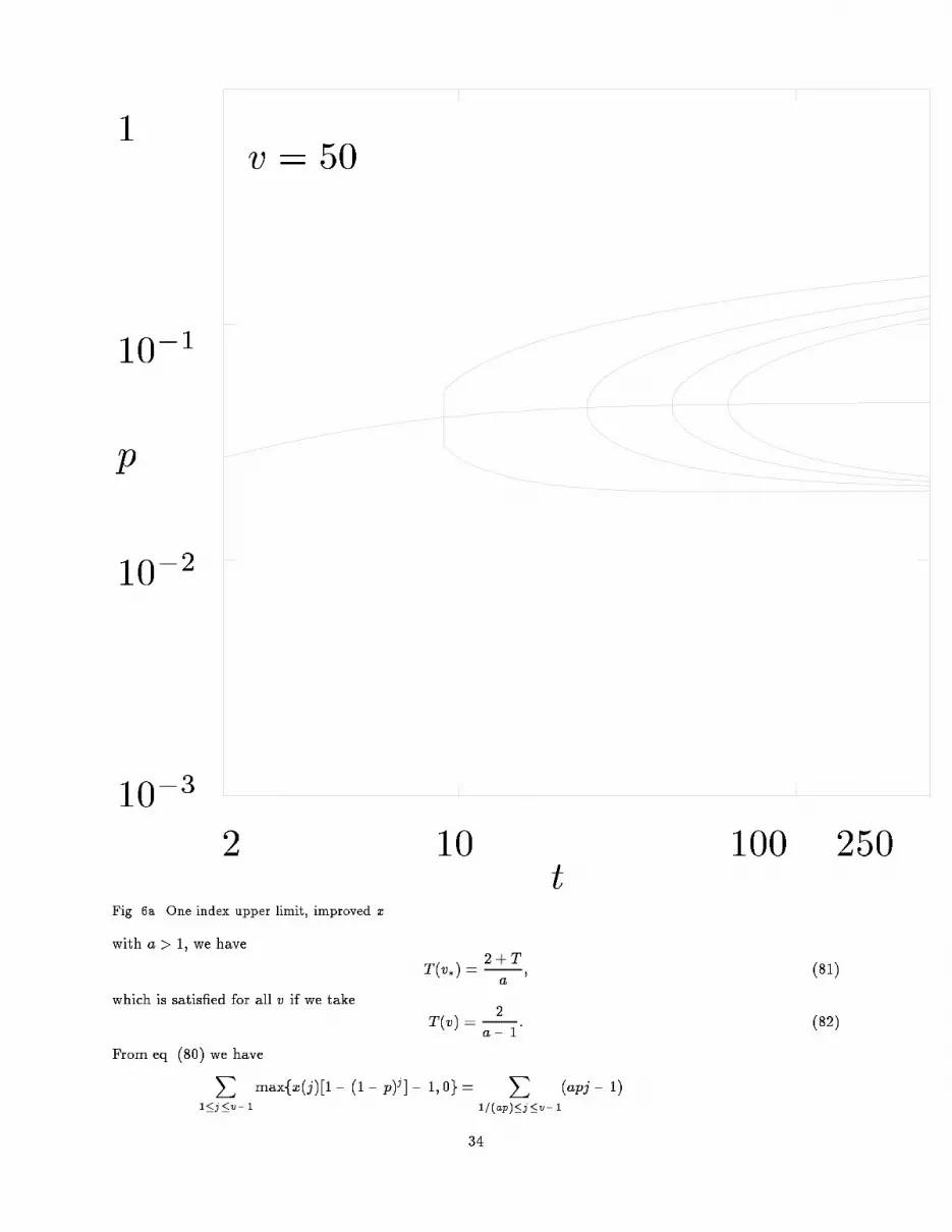
2 10 100 250tFig. 6a. One index upper limit, improved x.with a > 1, we have T (v�) = 2 + Ta ; (81)which is satis�ed for all v if we take T (v) = 2a� 1 : (82)From eq. (80) we haveX1�j�v�1maxfx(j)[1� (1� p)j]� 1; 0g = X1=(ap)�j�v�1(apj � 1)34

p110�110�210�3

v = 50

2 10 100 250tFig. 7. Zero index upper limit. � apv(v � 1)2 � (1=(ap)� 1)2 ��v � 1ap� : (83)Eq. (73) implies the average number of nodes is bounded by1 + 2a� 1 �1 + (1� p)v �1=a+ p2 � 1 + (a� 1)pv + ap2v(v � 1)2 ��t : (84)The derivative of this equation is cubic in a, but if we replace the 1=a term with one, then the derivative is35

a linear function. This suggests usinga = 2 + (1� p)v[�1 + p+ 2(t� 1)pv + p2tv(v � 1)]p(t � 1)v(1 � p)v[p(v � 1) + 2] (85)in eq. (84).Details: A Maple calculation shows that the derivative of (84) gives an equation that is cubic in a.The a that minimizes1 + 2a � 1 �1 + (1� p)v�1 + p2 � 1 + (a� 1)pv + ap2v(v � 1)2 ��tis given by eq. (85).�Figure 8 shows the bounds that result from eqs. (84, 85).9 AsymptoticsSince eqs. (84, 85) are more complex than eq. (79) the asymptotic analysis is based on eq. (79). Werequire that the bound on the number of nodes be no more than vn. That is,vn � 1 + 2v �1 + (1 � p)v �p2v(v � 1)2 � 1� p2 ��t ; (86)or vn�12 �1� 1vn� � �1 + (1� p)v�p2v(v � 1)2 � 1� p2 ��t : (87)9.1 Small tSolving for t in bound (87) givest � (n� 1) lnv � ln 2��(1=vn)lnf1 + [p2v(v � 1)� 1 + p](1� p)v=2g : (88)Details: From eq. (87)ln�vn�12 �1� 1vn�� � t ln�1 + (1� p)v �p2v(v � 1)2 � 1� p2 �� :Also ln�vn�12 �1� 1vn�� = (n� 1) lnv � ln 2��� 1vn� :� For n > 1 and 1 < a � pv � b <1, (88) can be simpli�ed tot � (n� 1) ln v � ln 2lnf1 + [(pv)2 � 1]e�pv=2g ; (89)which is bound (4).Details: Since pv � b(1� p)v = ev ln(1�p) = e�pve�v�(p2) = e�pv[1��(p)];ln�1 + (1� p)v p2v(v � 1)� 1 + p2 � = ln�1 + e�pv (pv)2 � 12 �1� �(p) ���1v���= ln�1 + e�pv (pv)2 � 12 �1� ��1v��� :36

p110�110�210�3

v = 50

2 10 100 250tFig. 8. Improved zero index upper limit.Now lnf1 + y[1 + �(x)]g = ln(1 + y)[1 + �(x)=(1 + y)]= ln(1 + y) + �(x)=(1 + y):Thus, when 1 < a � y � b <1 lnf1 + y[1 + �(x)]g = ln(1 + y) + �(x)and 1lnf1 + y[1 + �(x)]g = 1� �(x)ln(1 + y) :37

Since (1� p)v p2v(v � 1)� 1 + p2is positive and bounded for 1 < a � pv � b <1 and large v, we have(n� 1) ln v � ln 2��(1=vn)lnf1 + (1� p)v[p2v(v � 1)� 1 + p]=2g = (n � 1) ln v � ln 2� �(1=vn) + �(1=v)lnf1 + [(pv)2 � 1]e�pv=2g :When n > 1 and v is large the �(1=v) term is more important than the �(1=vn) term and since this is anupper bound, positive � terms can be dropped.�9.2 Small pFrom bound (87) using algebra, x = eln x, and power series we obtain(1� p)v[p2v(v � 1)� 1 + p] � 2[(n� 1) ln v � ln 2]t �1 + �� lnvt �� : (90)Details: 1 + (1 � p)v �p2v(v � 1)2 � 1� p2 � � v(n�1)=t21=t �1��� 1vnt��� e[(n�1) ln v�ln 2��(1=vn)]=t� 1 + (n � 1) lnv � ln 2t �1 + �� ln vt �� :Thus, (1 � p)v �p2v(v � 1)2 � 1� p2 � � (n� 1) lnv � ln 2t �1 + �� lnvt �� :� When pv > 1 and p2v is bounded, bound (90) can be written as[(pv)2 � 1]e�pv � 2[(n� 1) ln v � ln 2]t �1 + ��1v�+ �(p2v) + �� ln vt �� : (91)Details: Twice the left side of bound (90) is(1� p)v[p2v(v � 1)� 1 + p] = (pv � 1)(pv + 1� p)e�pve��(p2v):Since pv > 1, we have pv+1�p = (pv+1)[1��(1=v)] and since p2v is bounded we have e��(p2v) = 1��(p2v).Thus, the left side of bound (90) is[(pv)2 � 1]e�pv �1� ��1v���(p2v)� ;and we can write bound (90) as bound (91).�When pv is near 1, bound (91) is equivalent topv � 1 + e[(n� 1) ln v � ln 2]t (92)which is equivalent to bound (3).Details: Bound (91) can be written asp2v2 � 1 + 2epv (n� 1) ln v � ln 2t �1 + ��1v�+�� lnvt �� :To �nd the solution near pv = 1, let pv = 1 + y, giving2y + y2 � 2e[1 + y + �(y2)] (n� 1) ln v � ln 2t �1 + ��1v�+�� lnvt �� :Thus, y � e[(n� 1) lnv � ln 2]t �1 + ��1v�+�� lnvt �� :Since this is an upper bound, we drop positive � terms to obtain bound (92). (There is no solution with pvbelow 1.) � 38

9.3 Large pIn the previous section we found a solution to bound (87) that has pv near 1. For large pv, (1 � p)vdecreases much more rapidly than (pv)2 increases. Bound (91) has the form (x2 � 1)e�x � y with small y.The large x solution is x � � ln y + 2 ln(� ln y) + �� ln(� ln y)� ln y � : (93)Details: Assume x = � ln y + 2 ln(� ln y) + z ln(� ln y)=(� ln y). Plugging into (x2 � 1)e�x � y gives[� lny + 2 ln(� ln y) + z ln(� ln y)=(� ln y)]2 � 1(� ln y)2+z=(� ln y) y = y:Dividing both sides by y and clearing fractions gives�1 + 2 ln(� lny)� lny + z ln(� ln y)(� ln y)2 �2 � 1(� lny)2 = (� ln y)z=(� lny):Taking logarithms, expanding the logarithms, and retaining the important terms gives4 ln(� lny)� lny �1 + �� ln(� ln y)� ln y �� = z ln(� ln y)� ln y :In the limit the right side is bigger for z > 4 and the left side is bigger for z � 4. Thus,x = � ln y + 2 ln(� ln y) + �� ln(� lny)� ln y �is a solution. (Also, there is no solution with larger x.)�When t increases more rapidly than ln v the solution to (91) ispv � ln t+ 2 ln ln t � ln lnv � ln(n� 1)� ln 2 + �� ln ln tln t � : (94)This is bound (1).Details: For eq. (93) we have� lny = ln t� ln ln v � ln(n� 1)� ln 2���1v�� �(p2v) ��� ln vt � ;and ln(� ln y) = ln ln t��� ln lnvln t �� ��p2vln t���� ln vt ln t� ;so, when t increases more rapidly than lnvpv � ln t+ 2 ln ln t� ln ln v � ln(n� 1)� ln 2��� ln ln vln t �� ��1v���(p2v) � �� lnvt �+ �� ln ln tln t � :Since this is a lower bound the negative � terms can be dropped.�39

9.4 Comparison with Simple BacktrackingWhen t=v is large, the results of the small p analysis are not very good. A better result can be obtainedby observing that the average running time for Probe Order Backtracking is no larger than that of SimpleBacktracking. (The proof that the average running time of Clause Order Backtracking is no larger than thatof Simple Backtracking [3, Theorem 1] also applies to Probe Order Backtracking.)We require that A.18 from [22], the bound for Simple Backtracking, be no more than vn. For this boundwe use M (v) = v and � = 0 and let q = � ln(1� p) to obtainvn � 1 + v exp �2(ln 2)v + ln2� ln 2q ln�1 + qtln 2�+ t ln�1� ln 2ln2 + qt�� : (95)This can be written asqv � 12 ln(qv) � 12 ln� tv�+ 1� ln ln 22 + q2 ln2 [(n� 1) lnv � ln 2]��� qvn�+ �� 1qt� : (96)Details: When qt is large, it is useful to write the right side of (95) as1 + v exp �2(ln2)v + ln 2� ln 2q ln�qt+ ln 2ln 2 �+ t ln� qtln 2 + qt��= 1 + v exp �2(ln2)v + ln2 + (ln2) ln ln 2q �� ln 2q + t� ln(qt+ ln2) + t ln(qt)�= 1 + v exp ��1q� [2(ln 2)qv + q ln 2 + (ln2) ln ln2� (qt+ ln2) ln(qt+ ln 2) + qt ln(qt)]�= 1 + v exp��1q��2(ln2)qv + q ln 2 + (ln 2) ln ln 2� (ln 2) ln(qt) � (qt + ln 2) ln�1 + ln 2qt ��� :Now (x+ ln 2) ln�1 + ln 2x � = (x + ln 2)" ln 2x � 12 � ln 2x �2 + �� 1x3�#= ln 2� (ln 2)22x +�� 1x2�+ (ln2)2x � �� 1x2�= ln 2 + �� 1x� ;so the right side is1 + v exp��1q��2(ln2)qv � ln 2 + (ln 2) ln ln 2� (ln 2) ln(qt) + q ln 2��� 1qt���Using this in bound (95), rearranging, taking logarithms, and multiplying by q gives(n� 1)q lnv � 2(ln2)qv � ln 2 + (ln2) ln ln2� (ln 2) ln(qt) + q ln 2� �� 1qt�+ �� qvn� :Writing qt as (qv)(t=v), separating qv terms, and dividing by 2 ln 2 gives (96).�When t=v > e the solution to bound (96) isqv � 12 ln� tv�+ 12 ln ln� tv�+ 1� ln 2� ln ln 22 + q2 ln2 [(n�1) lnv� ln 2]+�� ln ln(t=v)ln(t=v) ���� qvn� : (97)Details: Consider the test solutionqv = 12 ln� tv�+ 12 ln ln� tv�+ 1� ln 2� ln ln 22 + q2 ln2 [(n� 1) lnv � ln 2] + a ln ln(t=v)ln(t=v) � �� qvn � :40

Assuming q lnv is smallln(qv) = ln ln� tv�� ln 2 + ln�1 + ln ln(t=v)ln(t=v) + �� 1ln(t=v)��= ln ln� tv�� ln 2 + ln ln(t=v)ln(t=v) + �� 1ln(t=v)� :Plugging the test solution into eq. (96) and simplifying givesa ln ln(t=v)ln(t=v) � ln ln(t=v)2 ln(t=v) � �� 1qt�+�� 1ln(t=v)� :The �(q=vn) terms cancel since they have the same implied constant. When t=v > e, ln ln(t=v) > 0. Thus,when t=v > e, the test solution, or anything smaller, works in the limit for any a < 1=2 giving bound (97).�Replacing q with its value in terms of p and solving for p in bound (97) givesp � � ln(t=v) + ln ln(t=v) + 1� ln 2� ln ln 22v �� �1 + 2(n � 1) lnv � (ln 2)[ln(t=v) + ln ln(t=v) + 3� ln 2� ln ln 2]4v ln 2��� (ln v) ln(t=v)v2 �� �� ln ln(t=v)v ln(t=v) �� (98)which is bound (2). For large v this is an improvement over the small p analysis when t = �v and � > 3:22136.Note that � > e.Details: Solving bound (97) for q givesq � � ln(t=v) + ln ln(t=v) + 1� ln 2� ln ln 22v +�� ln ln(t=v)v ln(t=v) ���1 + (n � 1) ln v � ln 22v ln 2 + �� (lnv)2v2 �� :From the de�nition of q q = � ln(1� p) = p+ p22 + p33 + �(p4):For small y, the solution, with p near y, top+ p22 + p33 + �(p4) = yis p = y h1� y2 + �(y2)i :Hence, solving for p in bound (97) givesp � � ln(t=v) + ln ln(t=v) + 1� ln 2� ln ln 22v + �� ln ln(t=v)v ln(t=v) ���1 + (n� 1) lnv � ln 22v ln 2 + ��(ln v)2v2 ��� �1� ln(t=v) + ln ln(t=v) + 1� ln 2� ln ln 24v � �� (lnv) ln(t=v)v2 �� �� ln ln(t=v)v ln(t=v) �+ ��� ln(t=v)v �2��:Multiplying the last two terms givesp � � ln(t=v) + ln ln(t=v) + 1� ln 2� ln ln 22v + �� ln ln(t=v)v ln(t=v) ��� �1 + 2(n� 1) lnv � 2 ln2� (ln 2)[ln(t=v) + ln ln(t=v) + 1� ln 2� ln ln 2]4v ln 2+ �� (lnv)2v2 �� �� (lnv) ln(t=v)v2 ���� ln ln(t=v)v ln(t=v) �+��� ln(t=v)v �2��:Since this is an upper limit, positive � terms can be dropped to give bound (98). �41

9.5 Comparison with Solution BoundaryThe average number of solutions to a random CNF Satis�ability problem is2v[1� (1 � p)v]t (99)[22, eq. A.1]. This is vn whenp = 1v �� ln�1� 1 + �(n(ln v)=t)e(ln 2)v=t �� [1��(p)] : (100)(Note that n = 0 corresponds to an average of one solution per problem.)Details: Setting formula (99) to vn, taking the tth root, and rearranging gives(1� p)v = 1� vn=t2v=t ;so pv = � ln�1� en(lnv)=te(ln 2)v=t� [1��(p)]= � ln�1� 1 + �(n(ln v)=t)e(ln 2)v=t � [1� �(p)] :� When t=v is large, this can be simpli�ed topv = (ln t� lnv � ln ln 2) �1� �� ln t� lnvv ��+ ��vt �+ ��n lnvv � : (101)Details: pv = � ln�1� �1 + ��n lnvt ���1� v ln 2t �1���vt ���� [1� �(p)]= � ln����n ln vt �+ v ln 2t h1���vt �i� [1��(p)]= � ln�v ln 2t �1���vt �+��n lnvv ��� [1� �(p)]= (ln t� lnv � ln ln 2) [1��(p)] + ��vt �+��n lnvv � :Thus pv = (ln t� lnv � ln ln 2) �1� �� ln t� lnvv ��+ ��vt �+ ��n lnvv � :� Note that for large t=v, the large p boundary for Probe Order Backtracking being fast (based on theupper bound analysis) is only slightly above the boundary for the number of solutions per problem beingabove 1. That is, the leading terms in eq. (94) are bigger than those in eq. (101) only by the amount ln v.When t=v is not large, the relative distance between the two curves increases.9.6 Intersection with Franco's AnalysisFranco gives an algorithm, [8], which makes selective use of resolution. This algorithm has the fastestproven average time for small t so long as p is not too large. Combining Franco's algorithm with Iwama'salgorithm [12] gives an algorithm that is fast for all p whent � O(n1=3(v= ln v)1=6): (102)42

The running time for Franco's algorithm is no more than3 + v + e�te�2p(1+p)v+(ln 2)[8(pt)3v+1]; (103)[8, pp 1123{1124]. To �nd the intersection with the upper bound analysis of Probe Order Backtracking, weuse bound (94) in Franco's bound (103) to eliminate p from the expression for the intersection point.3 + v + exp(��n � 1t ln t ��(1) + (8 ln2)t3(ln t)3v2 �1 + 2 ln ln tln t � ln lnvln t ��� ln(n� 1)ln t ��3 + ln 2) : (104)Details: Eq. (94) can be written aspv � ln t+ 2 ln ln t � ln lnv ��(ln(n � 1)) = ln� t(ln t)2�(n � 1) lnv � :When pv is equal to the bounde�2p(1+p)v = e�(2+2p)pv = � (n� 1)�(1) lnvt(ln t)2 �2+�(p) :When v and t are polynomially related ln t = �(ln v) so we may write this ase�2p(1+p)v = 1t2+�(p) �(n � 1)�(1)�(1) ln t �2+�(p) = 1t2+�(1) �n� 1ln t ��(1) :Plugging this and the value for p into Franco's bound gives eq. (104).�The bound (104) is no more than vn whent = 3n1=3v2=34(ln2)1=3(ln v)2=3 �1��� ln ln vlnv �� : (105)Details: Setting eq. (104) to vn and taking logarithms givesn ln v � �� 1vn�1� = ��n� 1t ln t ��(1) + (8 ln2)t3(ln t)3v2 �1 + 2 ln ln tln t � ln ln vln t ��� ln(n � 1)ln t ��3 + ln2;8(ln2)t3(ln t)3v2 �1 + 2 ln ln tln t � ln ln vln t ��� ln(n � 1)ln t ��3 = n lnv ��(1);t3(ln t)3 = nv2 lnv8 ln2 �1� �� 1lnv���1 + 2 ln ln tln t � ln lnvln t ��� ln(n� 1)ln t ���3 :We may write t ln t = (n lnv)1=3v2=32(ln2)1=3 �1��� 1ln v���1 + 2 ln ln tln t � ln lnvln t � �� 1ln t���1= (n lnv)1=3v2=32(ln2)1=3 �1��� 1ln v���1� 2 ln ln tln t + ln lnvln t + �� 1ln t��= (n lnv)1=3v2=32(ln2)1=3 �1� 2 ln ln tln t + ln ln vln t +�� 1ln t�� �� 1ln v�� :De�ne y = (n lnv)1=3v2=32(ln 2)1=3 �1� 2 ln ln tln t + ln lnvln t + �� 1ln t���� 1ln v��43

and solve y = t ln t for t. Consider the test solutiont = yln y "1 + ln lnyln y + a� ln lnyln y �2# :Plugging this in givesy = ylny "1 + ln ln yln y + a� ln ln yln y �2# ln( ylny "1 + ln ln yln y + a� ln ln yln y �2#)= y "1 + ln lnylny + a� ln lnylny �2# �1� ln ln yln y + ln ln y(ln y)2 +�� (a� 1=2)(ln lny)2(ln y)3 ��= y "1 + (a � 1)� ln lnyln y �2 +�� ln ln y(ln y)2�# :In the limit the left side is larger for a < 1 and the right side is larger for a > 1, so a solution ist = yln y �1 + ln ln ylny + ��(ln lny)2(ln y)2 �� :We have lny = 2 lnv3 + ln ln v3 + �(lnn) = 2 ln v3 �1 + ln ln v2 ln v + �� lnnlnv��and ln ln y = ln lnv +�(1);so t = 3(n lnv)1=3v2=34(ln2)1=3 ln v 1� (2 ln ln t)= ln t+ (ln lnv)= ln t+ �(1= ln t)� �(1= lnv)1 + (ln ln v)=(2 ln v) + �((lnn)= ln v)� �1 + 3 ln lnv + �(1)2 ln v + �(ln lnv) + �� (ln ln v)2(ln v)2 ��= 3(n lnv)1=3v2=34(ln2)1=3 ln v �1� 2 ln ln tln t + ln lnv2 ln t + �� 1ln t����1 + lnnln v ��� �1 + 3 ln lnv2 lnv +�� 1ln v��= 3(n lnv)1=3v2=34(ln2)1=3 ln v �1� 2 ln ln tln t + ln lnv2 ln t + 3 ln lnv2 ln v + �� 1ln t����1 + lnnln v �� :Since t is approximately v2=3, �2 ln ln tln t + ln ln v2 ln t + 3 ln ln v2 lnvis approximately �(3=4)(ln lnv)= ln v. Therefore the value of t reduces to eq. (105). �References1. Cynthia A. Brown and Paul W. Purdom, An Average Time Analysis of Backtracking, SIAM J. Comput.10 (1981) pp 583{593.2. Khaled Bugrara and Cynthia Brown, The Average Case Analysis of Some Satis�ability Model Problems,Information Sciences 40 (1986) pp 21{38.3. Khaled Bugrara and Paul Purdom, Average Time Analysis of Clause Order Backtracking, SIAM J.Comput. 23 (1993) pp 303{317.4. Khaled Bugrara, Youfang Pan, and Paul Purdom, Exponential Average Time for the Pure Literal Rule,SIAM J. Comput. 18 (1988) pp 409{418. 44

5. Michael Buro and Hans Kleine B�uning, Report on a SAT Competition, Bulletin of the European Asso-ciation for Theoretical Computer Science 49 (1993) pp 143{151.6. John Franco, On the Probabilistic Performance of Algorithms for the Satis�ability Problem, InformationProcessing Letters 18 (1986) pp 103{106.7. John Franco, On the Occurrence of Null Clauses in Random Instances of Satis�ability, Indiana Univer-sity Computer Science Tech. Report 291 (1989).8. John Franco, Elimination of Infrequent Variables Improves Average Case Performance of Satis�abilityAlgorithms, SIAM J. Comput. 20 (1991) pp 1119{1127.9. Allen Goldberg, Average Case Complexity of the Satis�ability Problem, Proc. Fourth Workshop onAutomated Deduction (1979) pp 1{6.10. Allen Goldberg, Paul Purdom, and Cynthia Brown, Average Time Analysis of Simpli�ed Davis-PutnumProcedures, Information Processing Letters 15 (1982) pp 72{75. Printer errors corrected in 16 (1983) p213.11. G. Neil Haven, unpublished analysis.12. Kazuo Iwama, CNF Satis�ability Test by Counting and Polynomial Average Time, SIAM J. Comput.18 (1989) pp 385{391.13. K. J. Lieberherr and E. Specker, Complexity of Partial Satisfaction, J. ACM 28 (1981) pp 411{421.14. Henri M. M�ejean, Henri Morel, G�erard Reynaud, \A Variational Method for Analysing Unit ClauseSearch", submitted for publication.15. Allen Newell and H. A. Simon, \GPS, A Program that Simulates Human Thought", Computers andThought (1963) pp 279{296, Edward A. Feigenbaum and Julian Feldman eds.16. Paul W. Purdom, Search Rearrangement Backtracking and Polynomial Average Time, Arti�cial Intelli-gence 21 (1983) pp 117{133.17. Paul W. Purdom, A Survey of Average Time Analyses of Satis�ability Algorithms, Journal of Informa-tion Processing, 13 (1990) pp 449{455. An earlier version appeared as Random Satis�ability Problems,Proc. of the International Workshop on Discrete Algorithms and Complexity, The Institute of Electron-ics, Information and Communication Engineers, Tokyo (1989) pp 253{259.18. Paul W. Purdom, Average Time for the Full Pure Literal Rule, Information Sciences, to appear.19. Paul W. Purdom, unpublished analysis.20. Paul W. Purdom and Cynthia A. Brown, An Analysis of Backtracking with Search Rearrangement,SIAM J. Comput. 12 (1983) pp 717{733.21. Paul W. Purdom and Cynthia A. Brown, The Pure Literal Rule and Polynomial Average Time, SIAMJ. Comput. 14 (1985) pp 943{953.22. Paul W. Purdom and Cynthia A. Brown, Polynomial-Average-Time Satis�ability Problems, InformationSciences 41 (1987) pp 23{42.23. Paul Walton Purdom Jr. and G. Neil Haven, Backtracking and Probing, Indiana University ComputerScience Technical Report No. 387 (1993).24. Rok Sosi�c and Jun Gu, Fast Search Algorithms for the N-Queens Problem, IEEE Trans. on Systems,Man, and Cybernetics 21 (1991) pp 1572{1576.45