arX

iv:1

103.

2765

v2 [

hep-

ph]

28

Mar

201

1

Probing the Tevatron tt asymmetry at LHC

J. A. Aguilar–Saavedra, M. Pérez-Victoria

Departamento de Física Teórica y del Cosmos and CAFPE,

Universidad de Granada, E-18071 Granada, Spain

Abstract

We use an effective operator framework to study the contributions to the

Tevatron tt asymmetry from arbitrary vector bosons and scalars, and compare

with their effect on the tt tail at LHC. Our study shows, for example, that models

reproducing the tt asymmetry by exchange of Z ′ and W ′ bosons or colour-triplet

scalars lead to a large enhancement in the tt tail at LHC. This fact can be used to

exclude these models as the sole explanation for the asymmetry, using the data

already collected by CMS and ATLAS. Our analysis is model independent in the

sense that we scan over all possible extra particles contributing to the asymmetry,

and allow for general couplings. We also explore a class of Standard Model ex-

tensions which can accommodate the Tevatron asymmetry without contributing

to the total tt cross section at first order, so that the enhancement of the tail at

Tevatron and LHC is moderate.

1 Introduction

The measurement of the tt forward-backward (FB) asymmetry at Tevatron [1–3] has

motivated a plethora of models which attempt to accommodate the experimental val-

ues, up to 3.4σ larger than the prediction of the Standard Model (SM). This task is

not straightforward because the measured tt cross section is in good agreement with

the SM: any “generic” addition to the tt production amplitude, large enough to pro-

duce the observed FB asymmetry, will easily give rise to too large a departure in the

total rate. Many of the proposed models circumvent this problem at the expense of

a cancellation between (linear) interference and (quadratic) new physics terms in the

total cross section,

σ(tt) = σSM + δσint + δσquad , (1)

where σSM is the SM cross section, δσquad the one corresponding to the new physics

and δσint the interference term. The cancellation δσint+δσquad ≃ 0 requires a new large

amplitude Anew ∼ −2ASM which, obviously, should have observable effects elsewhere.

The ideal candidate to search for these effects is the Large Hadron Collider (LHC).

1

New physics in uu, dd→ tt which produces such a large cancellation in the Tevatron

cross section will likely produce an observable enhancement in the tt tail at LHC,

even if at this collider top pair production is dominated by gluon fusion. (The tail

is also enhanced at Tevatron energies but in the majority of the proposed models the

deviations are compatible with present measurements [3].) In some cases, this effect

should be visible already with the data collected in 2010. Conversely, if large deviations

are not reported, a number of candidates to explain the Tevatron tt asymmetry will be

excluded from the list.

In this paper we make these arguments quantitative for a wide class of SM exten-

sions. We consider general new vector bosons and scalars, classified by their transfor-

mation properties under the SM gauge group SU(3)×SU(2)L×U(1)Y , and study their

possible effects in tt production. We use effective field theory to consistently (i) inte-

grate out the new heavy states and obtain their contribution to uu, dd → tt in terms

of four-fermion operators; (ii) obtain the cross sections in terms of effective operator

coefficients. This allows us to find, for each vector boson and scalar representation, a

relation between the possible values of the asymmetry AFB at Tevatron and the excess

in the tt tail at LHC. The discussion of all possible vector boson and scalar represen-

tations within the model-independent effective operator framework allows us to make

stronger statements than in other model-independent studies [4–7]. At the same time,

any model with several vector bosons and scalars can be considered in our framework

by simply summing the effective operator coefficients corresponding to the integration

of each new particle. Previous studies of LHC signals associated to the FB asymmetry

within particular models have been presented in Refs. [8–16].

After this analysis, we explore an alternative way to produce a large asymmetry with

moderate effects in the tt tail at LHC. The key for this mechanism is the observation

that one can also obtain a large AFB without significant changes in the total tt cross

section by introducing new physics which only contributes to the latter at quadratic

order. This has been studied before, in the effective formalism, in Ref. [5]. If we write

σF (tt) = σFSM + σF

int + σFquad ,

σB(tt) = σBSM + σB

int + σBquad , (2)

for the forward (F) and backward (B) cross sections, the total rate is maintained at first

order provided σFint + σB

int ≃ 0, which can be achieved, for example, with a new vector

boson and a scalar. For models fulfilling this cancellation the size of the new physics

contributions required to accommodate the experimental value of AFB are smaller.

Therefore, these models provide a better agreement of the tt tail with Tevatron mea-

surements, and predict a much smaller tail at LHC, which is still potentially observable

2

with forthcoming measurements.

We remark that the use of effective field theory (with the assumption that the new

physics is too heavy to be directly produced at LHC) does not limit much the generality

of our conclusions. For t-channel exchange of new vector bosons or scalars, integrating

out the new particles gives a good estimate for masses M & 1 TeV. For s-channel

exchange this approximation is worse, but the cross section enhancement produced by

the new particle(s) is always larger than the one from the corresponding four-fermion

operator(s), and in this sense our predictions are conservative. On the other hand, if

new physics in the tt tail is not seen at LHC, the new resonances are heavy and the

effective operator framework can be safely used. It is also worth pointing out that

we include 1/Λ4 corrections arising from the quadratic terms in new physics in the

cross sections. The contributions from the interference of 1/Λ4 operators with the SM

can be neglected, as they are suppressed with respect to the former for the values of

parameters that are required to explain the tt asymmetry.

2 Extra bosons, operators and tt production

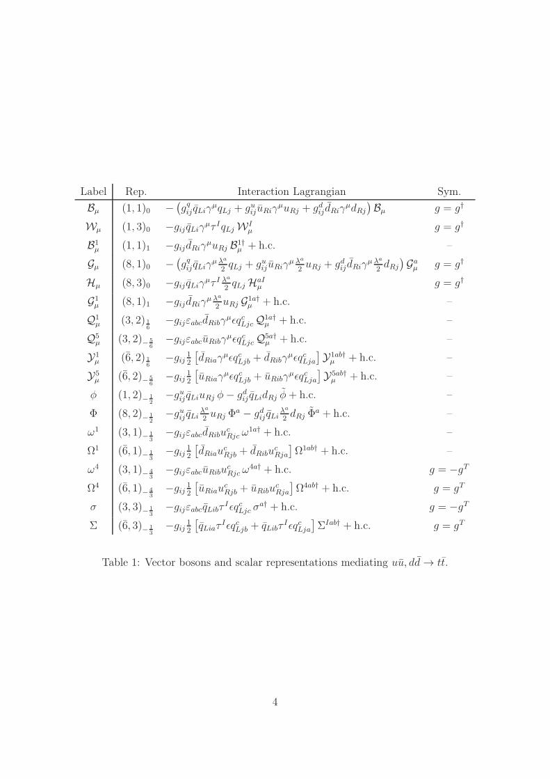
There are ten possible SU(3) × SU(2)L × U(1)Y representations [17] for new vector

bosons contributing to uu, dd → tt, while for scalars eight representations contribute.

They are collected in Table 1, where the first column indicates the label used to refer

to them.1 The relevant interaction Lagrangian is included as well, indicating the sym-

metry properties, if any, of the coupling matrices gij. We use standard notation with

left-handed doublets qLi and right-handed singlets uRi, dRi; τI are the Pauli matrices,

λa the Gell-Mann matrices normalised to tr(λaλb) = 2δab and φ = ǫφ, ψc = CψT , with

ǫ = iτ 2 and C the charge conjugation matrix. The indices a, b, c denote colour, and

εabc is the totally antisymmetric tensor.

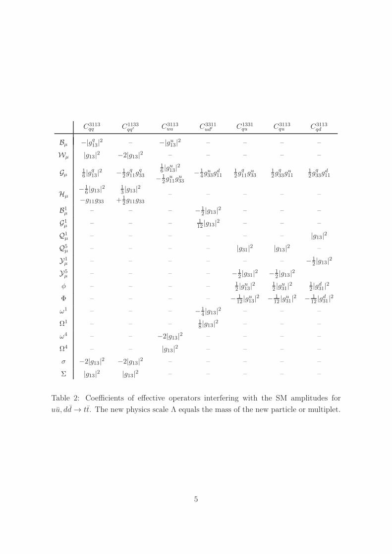
The four-fermion operators contributing to tt production, including those that do

not interfere with the SM QCD amplitude and only appear at quadratic level, have

been given in Ref. [18]. (The operators which interfere with the SM were given in

Ref. [19].) We collect in Tables 2–5 the values of the corresponding coefficients for all

the vector and scalar irreducible representations that can induce these operators. For

vector bosons the coefficients have previously been obtained in Ref. [17]. The notation

for four-fermion operators is given in appendix A. We stress again that including both

interference 1/Λ2 and quadratic 1/Λ4 terms in our calculations is not inconsistent,

1We note that for Wµ and Hµ the normalisation in the Lagrangian differs from Ref. [17] by a factor

of two, to simplify the presentation of the limits.

3

Label Rep. Interaction Lagrangian Sym.

Bµ (1, 1)0 −(

gqij qLiγµqLj + guijuRiγ

µuRj + gdijdRiγµdRj

)

Bµ g = g†

Wµ (1, 3)0 −gij qLiγµτ IqLj WIµ g = g†

B1

µ (1, 1)1 −gijdRiγµuRj B1†

µ + h.c. –

Gµ (8, 1)0 −(

gqij qLiγµ λa

2qLj + guijuRiγ

µ λa

2uRj + gdij dRiγ

µ λa

2dRj

)

Gaµ g = g†

Hµ (8, 3)0 −gij qLiγµτ I λa

2qLj HaI

µ g = g†

G1

µ (8, 1)1 −gijdRiγµ λa

2uRj G1a†

µ + h.c. –

Q1

µ (3, 2) 16

−gijεabcdRibγµǫqcLjcQ1a†

µ + h.c. –

Q5

µ (3, 2)− 56

−gijεabcuRibγµǫqcLjcQ5a†

µ + h.c. –

Y1

µ (6, 2) 16

−gij 12[

dRiaγµǫqcLjb + dRibγ

µǫqcLja]

Y1ab†µ + h.c. –

Y5

µ (6, 2)− 56

−gij 12[

uRiaγµǫqcLjb + uRibγ

µǫqcLja]

Y5ab†µ + h.c. –

φ (1, 2)− 12

−guij qLiuRj φ− gdij qLidRj φ+ h.c. –

Φ (8, 2)− 12

−guij qLi λa

2uRj Φ

a − gdij qLiλa

2dRj Φ

a + h.c. –

ω1 (3, 1)− 13

−gijεabcdRibucRjc ω

1a† + h.c. –

Ω1 (6, 1)− 13

−gij 12[

dRiaucRjb + dRibu

cRja

]

Ω1ab† + h.c. –

ω4 (3, 1)− 43

−gijεabcuRibucRjc ω

4a† + h.c. g = −gT

Ω4 (6, 1)− 43

−gij 12[

uRiaucRjb + uRibu

cRja

]

Ω4ab† + h.c. g = gT

σ (3, 3)− 13

−gijεabcqLibτ IǫqcLjc σa† + h.c. g = −gT

Σ (6, 3)− 13

−gij 12[

qLiaτIǫqcLjb + qLibτ

IǫqcLja]

ΣIab† + h.c. g = gT

Table 1: Vector bosons and scalar representations mediating uu, dd→ tt.

4

C3113qq C1133

qq′ C3113uu C3311

ud′ C1331qu C3113

qu C3113

qd

Bµ −|gq13|2 – −|gu

13|2 – – – –

Wµ |g13|2 −2|g13|2 – – – – –

Gµ1

6|gq

13|2 −1

2gq11gq33

1

6|gu

13|2

−1

2gu11gu33

−1

4gu33gd11

1

2gq11gu33

1

2gq33gu11

1

2gq33gd11

Hµ

−1

6|g13|2

−g11g33

1

3|g13|2

+1

2g11g33

– – – – –

B1µ – – – −1

2|g13|2 – – –

G1µ – – – 1

12|g13|2 – – –

Q1µ – – – – – – |g13|2

Q5µ – – – – |g31|2 |g13|2 –

Y1µ – – – – – – −1

2|g13|2

Y5µ – – – – −1

2|g31|2 −1

2|g13|2

φ – – – – 1

2|gu

13|2 1

2|gu

31|2 1

2|gd

31|2

Φ – – – – − 1

12|gu

13|2 − 1

12|gu

31|2 − 1

12|gd

31|2

ω1 – – – −1

4|g13|2 – – –

Ω1 – – – 1

8|g13|2 – – –

ω4 – – −2|g13|2 – – – –

Ω4 – – |g13|2 – – – –

σ −2|g13|2 −2|g13|2 – – – – –

Σ |g13|2 |g13|2 – – – – –

Table 2: Coefficients of effective operators interfering with the SM amplitudes for

uu, dd→ tt. The new physics scale Λ equals the mass of the new particle or multiplet.

5

C1133

qq C3113

qq′ C1133

uu C3311

ud

Bµ −gq11gq33

– −gu11gu33

−1

2gu33gd11

Wµ gq11gq33

−2gq11gq33

– –

Gµ1

6gq11gq33

−1

2|gq

13|2

1

6gu11gu33

−1

2|gu

13|2

1

12gu33gd11

Hµ

−1

6g11g33

−|g13|21

2|g13|2

+1

3g11g33

– –

G1

µ – – – −1

4|g13|2

ω1 – – – 1

4|g13|2

Ω1 – – – 1

8|g13|2

ω4 – – 2|g13|2 –

Ω4 – – |g13|2 –

σ 2|g13|2 2|g13|2 – –

Σ |g13|2 |g13|2 – –

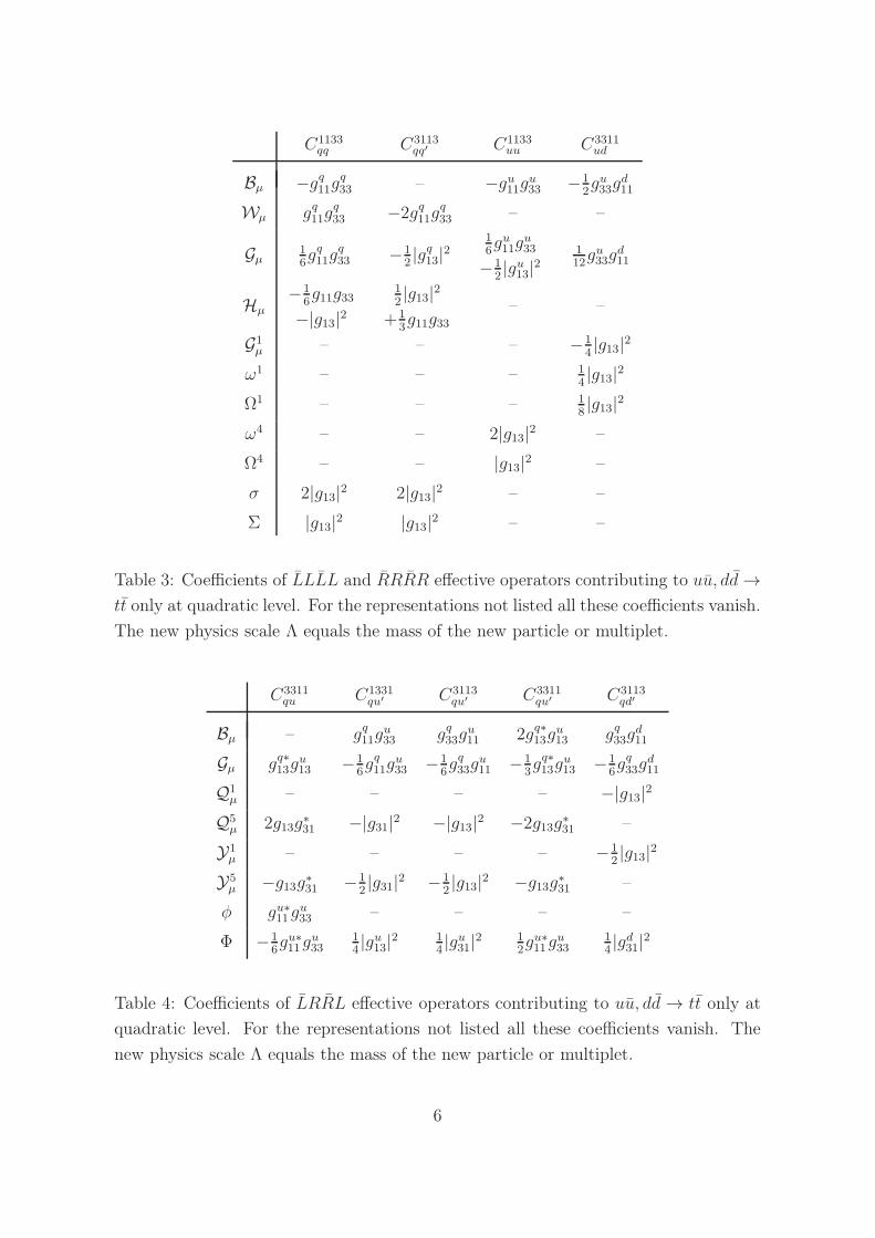
Table 3: Coefficients of LLLL and RRRR effective operators contributing to uu, dd→tt only at quadratic level. For the representations not listed all these coefficients vanish.

The new physics scale Λ equals the mass of the new particle or multiplet.

C3311

qu C1331

qu′ C3113

qu′ C3311

qu′ C3113

qd′

Bµ – gq11gu33

gq33gu11

2gq∗13gu13

gq33gd11

Gµ gq∗13gu13

−1

6gq11gu33

−1

6gq33gu11

−1

3gq∗13gu13

−1

6gq33gd11

Q1

µ – – – – −|g13|2

Q5

µ 2g13g∗31

−|g31|2 −|g13|2 −2g13g∗31

–

Y1

µ – – – – −1

2|g13|2

Y5

µ −g13g∗31 −1

2|g31|2 −1

2|g13|2 −g13g∗31 –

φ gu∗11gu33

– – – –

Φ −1

6gu∗11gu33

1

4|gu

13|2 1

4|gu

31|2 1

2gu∗11gu33

1

4|gd

31|2

Table 4: Coefficients of LRRL effective operators contributing to uu, dd → tt only at

quadratic level. For the representations not listed all these coefficients vanish. The

new physics scale Λ equals the mass of the new particle or multiplet.

6

C1331

qqǫ C3311

qqǫ C1331

qqǫ′ C3311

qqǫ′

φ gu13gd31

gu33gd11

– –

Φ −1

6gu13gd31

−1

6gu33gd11

1

2gu13gd31

1

2gu33gd11

Table 5: Coefficients of LRLR effective operators contributing to uu, dd → tt only at

quadratic level. For the representations not listed all these coefficients vanish. The

new physics scale Λ equals the mass of the new particle or multiplet.

despite the fact that we are not considering dimension-eight operators. When quadratic

terms are relevant for tt production (large couplings) the missing dimension-eight terms

are sub-leading in the classes of SM extensions we consider. A related discussion about

the importance of 1/Λ2 and 1/Λ4 contributions from dimension-six operators has been

presented in Ref. [20].

We evaluate the FB asymmetry

AFB =σF − σB

σF + σB=σF

SM + δσF − σBSM − δσB

σFSM + δσF + σB

SM + δσB, (3)

using the SM predictions [21]

ASMFB = 0.058± 0.009 (inclusive) ,

ASMFB = 0.088± 0.013 (mtt > 450 GeV) . (4)

and the new contributions from four-fermion operators δσF,B, parameterised in terms

of effective operator coefficients and numerical constants. The explicit expressions are

collected in appendix A. It is important to point out that positive operator coeffi-

cients always increase AFB at first order (1/Λ2 interference with the SM), as it follows

from Eqs. (13). We choose, among the recently reported measurements of the FB

asymmetry [3],

AexpFB = 0.158± 0.075 (inclusive) ,

Aexp

FB = 0.475± 0.114 (mtt > 450 GeV) . (5)

the one for high tt invariant masses which exhibits the largest deviation (3.4σ) with

respect to the SM prediction. The total cross section at LHC is evaluated including

four-fermion operators in a similar way. In order to display the effect of new contribu-

tions on the tt tail we evaluate the cross section for tt invariant masses larger than 1

TeV. We note that our calculation in terms of effective operators gives a larger (smaller)

tail than the exact calculation for t-channel (s-channel) resonances. In the former case

7

the differences are not dramatic but in the latter our results can be quite conservative,

depending on the mass and width of the new resonance. A detailed comparison is

presented in appendix B.

0.5 1 1.5 2 2.5 3 3.5 4 4.5 5σ / σ

SM (m

tt> 1 TeV)

-0.2

-0.1

0

0.1

0.2

0.3

0.4

AFB

(m

tt>

450

GeV

)

B µW µ

0.5 1 1.5 2 2.5 3 3.5 4 4.5 5σ / σ

SM (m

tt> 1 TeV)

-0.4

-0.2

0

0.2

0.4

0.6

AFB

(m

tt>

450

GeV

)

G µH µ

0.5 1 1.5 2 2.5 3 3.5 4 4.5 5σ / σ

SM (m

tt> 1 TeV)

0

0.05

0.10

0.15

0.20

AFB

(m

tt>

450

GeV

)

B µ1

G µ1

0.5 1 1.5 2 2.5 3 3.5 4 4.5 5σ / σ

SM (m

tt> 1 TeV)

-0.1

-0.05

0

0.05

0.1

0.15

0.2

AFB

(m

t t>

450

GeV

)

Q µ1

Y µ1

0.5 1 1.5 2 2.5 3 3.5 4 4.5 5σ / σ

SM (m

tt> 1 TeV)

-0.3

-0.2

-0.1

0

0.1

0.2

0.3

AFB

(m

tt>

450

GeV

)

Q µ5

Y µ5

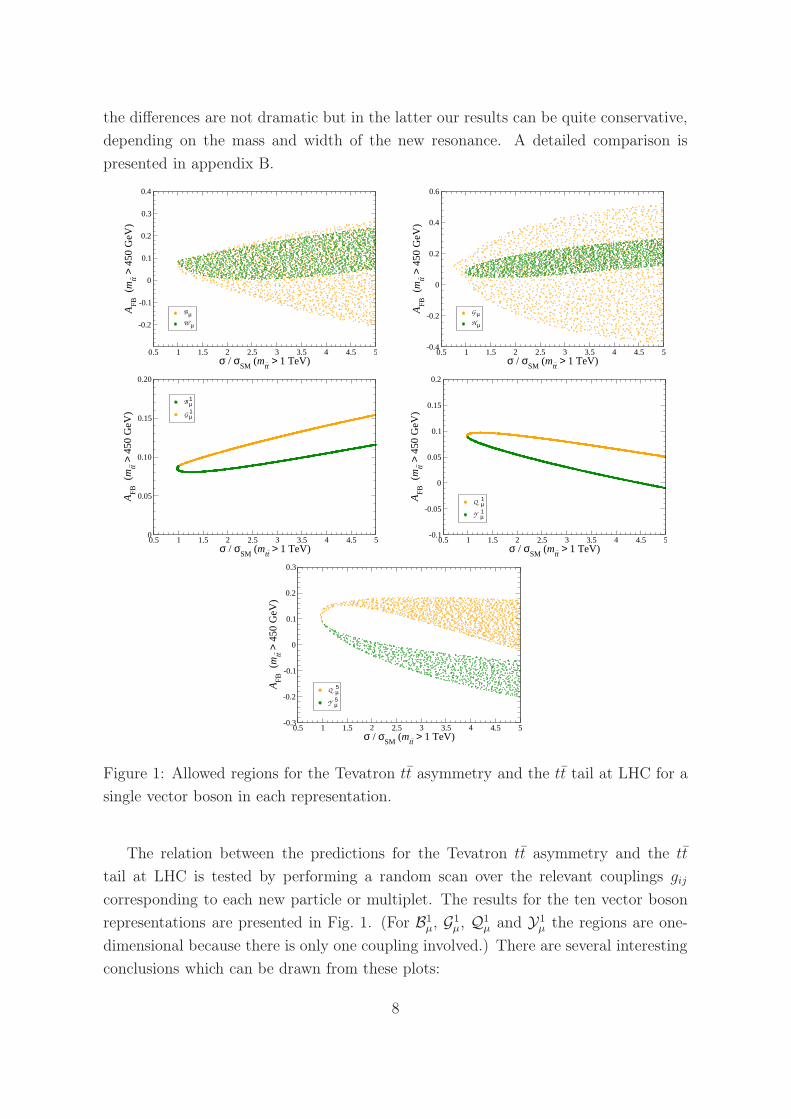
Figure 1: Allowed regions for the Tevatron tt asymmetry and the tt tail at LHC for a

single vector boson in each representation.

The relation between the predictions for the Tevatron tt asymmetry and the tt

tail at LHC is tested by performing a random scan over the relevant couplings gij

corresponding to each new particle or multiplet. The results for the ten vector boson

representations are presented in Fig. 1. (For B1

µ, G1

µ, Q1

µ and Y1

µ the regions are one-

dimensional because there is only one coupling involved.) There are several interesting

conclusions which can be drawn from these plots:

8

1. For Wµ and Hµ the allowed regions are inside the corresponding ones for Bµ, Gµ,

respectively. This is expected because the interactions of the former correspond

to a particular case of the latter, with only left-handed couplings.

2. For new colour-singlet neutral bosons Bµ, Wµ the linear terms have negative

coefficients and decrease AFB, which can only reach the experimental value for

large couplings when quadratic terms dominate. Hence, accommodating a large

asymmetry automatically implies a large tt tail. For example, for AFB & 0.3

the enhancement is more than a factor of five. This implies that these possible

explanations for AFB can be probed, and eventually excluded, with the luminosity

collected in the 2010 run of LHC. The same conclusion applies to the vector

bosons G1

µ and B1

µ, as they only contribute in dd initial states and require a huge

coupling to produce a large asymmetry.

3. For colour-octet isosinglet bosons Gµ it is possible to have a large AFB and still a

moderate tail at LHC. This model provides an example of cancellation of linear

1/Λ2 terms in the cross section, provided that gqii = −guii = −gdii, i.e. the vector

boson couples as an axigluon. However, in order to have positive coefficients in

the interference terms the couplings for the third and first generation must have

opposite sign. This does not happen for the isotriplet boson Hµ which only has

left-handed couplings, and for these SM extensions the predicted tt tail is large.

4. Another interesting candidate is a colour triplet Q5

µ, which has positive coeffi-

cients in interference terms as well. Its inclusion gives some enhancement to the

asymmetry, which can reach the experimental value with the further addition of a

scalar. Note that quadratic terms from operators Oqu(′) decrease the asymmetry,

as it can be derived from Eqs. (14) and is clearly seen in Fig. 1. Hence, this

model is interesting only for moderate couplings.

5. The rest of vector bosons, Q1

µ, Y1

µ and Y5

µ have little interest for the tt asymmetry

because they do not allow for a value appreciably larger than the SM prediction.

Aside from these remarks, we also note that for (i) B1

µ and G1

µ; (ii) Q1

µ and Y1

µ; (iii)

Q5

µ and Y5

µ, the linear 1/Λ2 terms have opposite sign, which explains the behaviour

observed in the plots for these vector bosons.

The results for the eight scalar representations are presented in Fig. 2. Except for

the isodoublets φ, Φ, the regions are one-dimensional because there is only one coupling

involved. We point out that:

9

0.5 1 1.5 2 2.5 3 3.5 4 4.5 5σ / σ

SM (m

tt> 1 TeV)

-0.3

-0.2

-0.1

0

0.1

0.2

0.3

0.4

AFB

(m

t t>

450

GeV

)

φΦ

0.5 1 1.5 2 2.5 3 3.5 4 4.5 5σ / σ

SM (m

tt> 1 TeV)

0

0.05

0.1

0.15

0.2

0.25

0.3

0.35

0.4

AFB

(m

tt>

450

GeV

)

Σσ

0.5 1 1.5 2 2.5 3 3.5 4 4.5 5σ / σ

SM (m

tt> 1 TeV)

0

0.05

0.10

0.15

0.20

AFB

(m

tt>

450

GeV

)

Ω1

ω1

0.5 1 1.5 2 2.5 3 3.5 4 4.5 5σ / σ

SM (m

tt> 1 TeV)

0

0.1

0.2

0.3

0.4

AFB

(m

t t>

450

GeV

)

Ω4

ω4

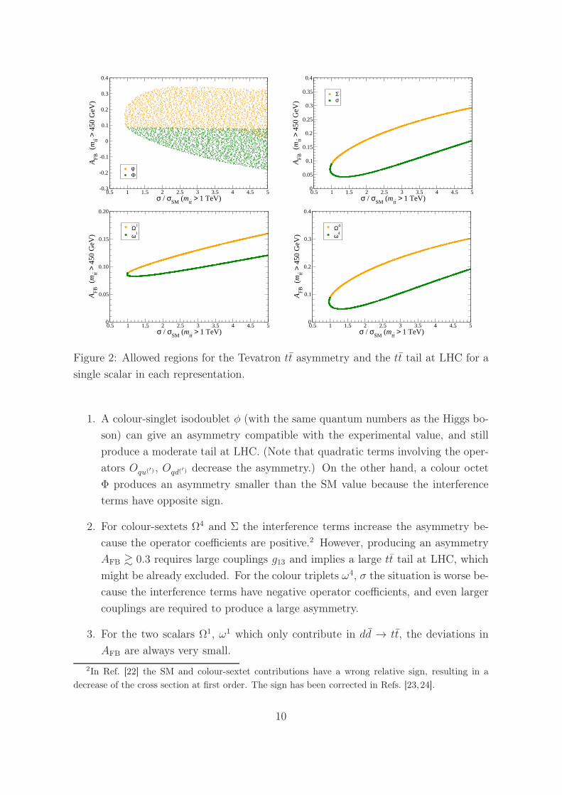
Figure 2: Allowed regions for the Tevatron tt asymmetry and the tt tail at LHC for a

single scalar in each representation.

1. A colour-singlet isodoublet φ (with the same quantum numbers as the Higgs bo-

son) can give an asymmetry compatible with the experimental value, and still

produce a moderate tail at LHC. (Note that quadratic terms involving the oper-

ators Oqu(′) , Oqd(′) decrease the asymmetry.) On the other hand, a colour octet

Φ produces an asymmetry smaller than the SM value because the interference

terms have opposite sign.

2. For colour-sextets Ω4 and Σ the interference terms increase the asymmetry be-

cause the operator coefficients are positive.2 However, producing an asymmetry

AFB & 0.3 requires large couplings g13 and implies a large tt tail at LHC, which

might be already excluded. For the colour triplets ω4, σ the situation is worse be-

cause the interference terms have negative operator coefficients, and even larger

couplings are required to produce a large asymmetry.

3. For the two scalars Ω1, ω1 which only contribute in dd → tt, the deviations in

AFB are always very small.

2In Ref. [22] the SM and colour-sextet contributions have a wrong relative sign, resulting in a

decrease of the cross section at first order. The sign has been corrected in Refs. [23, 24].

10

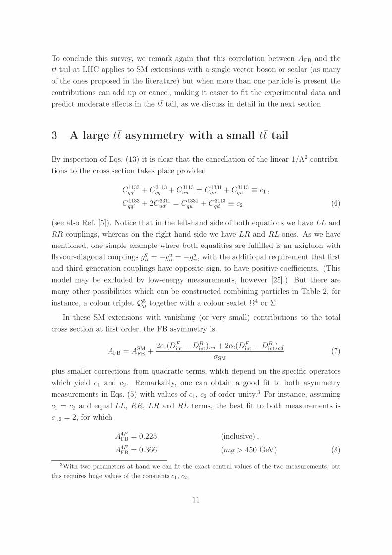
To conclude this survey, we remark again that this correlation between AFB and the

tt tail at LHC applies to SM extensions with a single vector boson or scalar (as many

of the ones proposed in the literature) but when more than one particle is present the

contributions can add up or cancel, making it easier to fit the experimental data and

predict moderate effects in the tt tail, as we discuss in detail in the next section.

3 A large tt asymmetry with a small tt tail

By inspection of Eqs. (13) it is clear that the cancellation of the linear 1/Λ2 contribu-

tions to the cross section takes place provided

C1133

qq′ + C3113

qq + C3113

uu = C1331

qu + C3113

qu ≡ c1 ,

C1133

qq′ + 2C3311

ud′ = C1331

qu + C3113

qd ≡ c2 (6)

(see also Ref. [5]). Notice that in the left-hand side of both equations we have LL and

RR couplings, whereas on the right-hand side we have LR and RL ones. As we have

mentioned, one simple example where both equalities are fulfilled is an axigluon with

flavour-diagonal couplings gqii = −guii = −gdii, with the additional requirement that first

and third generation couplings have opposite sign, to have positive coefficients. (This

model may be excluded by low-energy measurements, however [25].) But there are

many other possibilities which can be constructed combining particles in Table 2, for

instance, a colour triplet Q5

µ together with a colour sextet Ω4 or Σ.

In these SM extensions with vanishing (or very small) contributions to the total

cross section at first order, the FB asymmetry is

AFB = ASMFB +

2c1(DFint −DB

int)uu + 2c2(DFint −DB

int)ddσSM

(7)

plus smaller corrections from quadratic terms, which depend on the specific operators

which yield c1 and c2. Remarkably, one can obtain a good fit to both asymmetry

measurements in Eqs. (5) with values of c1, c2 of order unity.3 For instance, assuming

c1 = c2 and equal LL, RR, LR and RL terms, the best fit to both measurements is

c1,2 = 2, for which

A4FFB = 0.225 (inclusive) ,

A4FFB = 0.366 (mtt > 450 GeV) (8)

3With two parameters at hand we can fit the exact central values of the two measurements, but

this requires huge values of the constants c1, c2.

11

300 400 500 600 700 800 900 1000m

tt (GeV)

0

0.2

0.4

0.6

0.8

1

σ (p

b) /

20 G

eVSM + 4FSM

Tevatron

300 400 500 600 700 800 900 1000m

tt (GeV)

10-3

10-2

10-1

1

σ (p

b) /

20 G

eV

SM + 4FSM

Tevatron

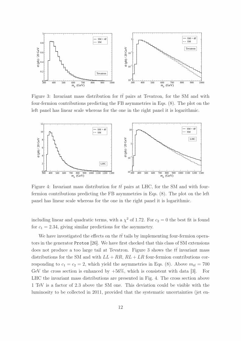
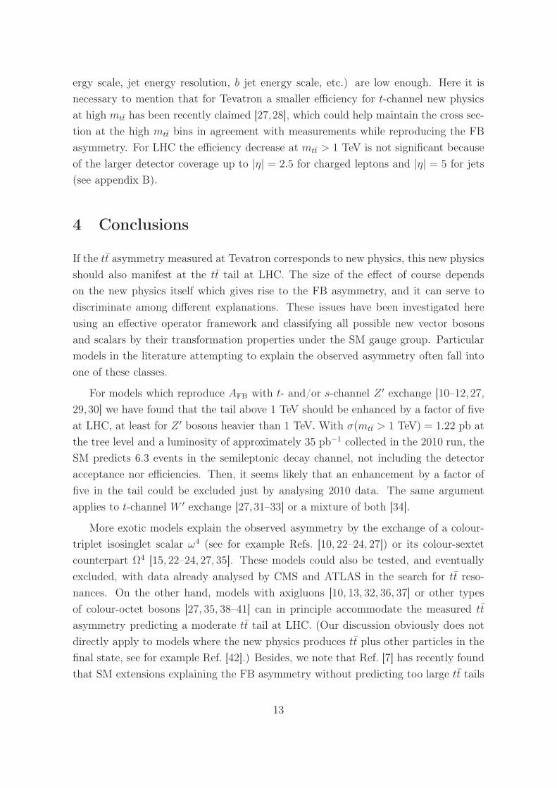
Figure 3: Invariant mass distribution for tt pairs at Tevatron, for the SM and with

four-fermion contributions predicting the FB asymmetries in Eqs. (8). The plot on the

left panel has linear scale whereas for the one in the right panel it is logarithmic.

300 400 500 600 700 800 900 1000 1100 1200 1300m

tt (GeV)

0

2

4

6

8

10

12

σ (p

b) /

20 G

eV

SM + 4FSM

LHC

300 400 500 600 700 800 900 1000 1100 1200 1300m

tt (GeV)

10-2

10-1

1

10

σ (p

b) /

20 G

eVSM + 4FSM

LHC

Figure 4: Invariant mass distribution for tt pairs at LHC, for the SM and with four-

fermion contributions predicting the FB asymmetries in Eqs. (8). The plot on the left

panel has linear scale whereas for the one in the right panel it is logarithmic.

including linear and quadratic terms, with a χ2 of 1.72. For c2 = 0 the best fit is found

for c1 = 2.34, giving similar predictions for the asymmetry.

We have investigated the effects on the tt tails by implementing four-fermion opera-

tors in the generator Protos [26]. We have first checked that this class of SM extensions

does not produce a too large tail at Tevatron. Figure 3 shows the tt invariant mass

distributions for the SM and with LL+RR, RL+LR four-fermion contributions cor-

responding to c1 = c2 = 2, which yield the asymmetries in Eqs. (8). Above mtt = 700

GeV the cross section is enhanced by +56%, which is consistent with data [3]. For

LHC the invariant mass distributions are presented in Fig. 4. The cross section above

1 TeV is a factor of 2.3 above the SM one. This deviation could be visible with the

luminosity to be collected in 2011, provided that the systematic uncertainties (jet en-

12

ergy scale, jet energy resolution, b jet energy scale, etc.) are low enough. Here it is

necessary to mention that for Tevatron a smaller efficiency for t-channel new physics

at high mtt has been recently claimed [27,28], which could help maintain the cross sec-

tion at the high mtt bins in agreement with measurements while reproducing the FB

asymmetry. For LHC the efficiency decrease at mtt > 1 TeV is not significant because

of the larger detector coverage up to |η| = 2.5 for charged leptons and |η| = 5 for jets

(see appendix B).

4 Conclusions

If the tt asymmetry measured at Tevatron corresponds to new physics, this new physics

should also manifest at the tt tail at LHC. The size of the effect of course depends

on the new physics itself which gives rise to the FB asymmetry, and it can serve to

discriminate among different explanations. These issues have been investigated here

using an effective operator framework and classifying all possible new vector bosons

and scalars by their transformation properties under the SM gauge group. Particular

models in the literature attempting to explain the observed asymmetry often fall into

one of these classes.

For models which reproduce AFB with t- and/or s-channel Z ′ exchange [10–12,27,

29,30] we have found that the tail above 1 TeV should be enhanced by a factor of five

at LHC, at least for Z ′ bosons heavier than 1 TeV. With σ(mtt > 1 TeV) = 1.22 pb at

the tree level and a luminosity of approximately 35 pb−1 collected in the 2010 run, the

SM predicts 6.3 events in the semileptonic decay channel, not including the detector

acceptance nor efficiencies. Then, it seems likely that an enhancement by a factor of

five in the tail could be excluded just by analysing 2010 data. The same argument

applies to t-channel W ′ exchange [27, 31–33] or a mixture of both [34].

More exotic models explain the observed asymmetry by the exchange of a colour-

triplet isosinglet scalar ω4 (see for example Refs. [10, 22–24, 27]) or its colour-sextet

counterpart Ω4 [15, 22–24, 27, 35]. These models could also be tested, and eventually

excluded, with data already analysed by CMS and ATLAS in the search for tt reso-

nances. On the other hand, models with axigluons [10, 13, 32, 36, 37] or other types

of colour-octet bosons [27, 35, 38–41] can in principle accommodate the measured tt

asymmetry predicting a moderate tt tail at LHC. (Our discussion obviously does not

directly apply to models where the new physics produces tt plus other particles in the

final state, see for example Ref. [42].) Besides, we note that Ref. [7] has recently found

that SM extensions explaining the FB asymmetry without predicting too large tt tails

13

must have interference with the SM amplitudes.4 As we have shown, our conclusions

are stronger because in many extensions with interference this is not possible either.

Moreover, for all vector bosons and scalars in Table 1 there is interference unless the

involved couplings vanish.

Finally, in this paper we have investigated the conditions under which the first

order 1/Λ2 contributions to the total tt cross section cancel while still producing a

FB asymmetry compatible with experimental data. (A previous study at this order

has been presented in Ref. [5].) Clearly, in this situation the tails of the tt invariant

mass distribution are much smaller, both at Tevatron and LHC, as it has been shown

explictly. A popular example of a model fulfilling these conditions is an axigluon

with opposite couplings to the first and third generation, but there are many other

possibilities which can be worked out from Table 2. All these SM extensions can

accommodate the Tevatron tt asymmetry and cross section with small couplings, and

predict a moderate enhancement of the tt tail at Tevatron and LHC, which is not in

contradiction with experiment. Interestingly, a small excess in the tt tail with boosted

tops has been already observed at Tevatron [43]. In any case, these possible departures

will soon be tested with forthcoming LHC data.

Acknowledgements

This work has been partially supported by projects FPA2010-17915 (MICINN), FQM

101 and FQM 437 (Junta de Andalucía) and CERN/FP/116397/2010 (FCT).

A Four-fermion operators in tt production

We use the minimal basis in Ref. [18] for gauge-invariant four-fermion operators.

Fermion fields are ordered according to their spinorial index contraction, and subindices

a, b indicate the pairs with colour indices contracted, if this pairing is different from

the one for the spinorial contraction. Our basis consists of the following operators:

4This reference has appeared in the arXiv one day before the present paper, and our findings are

consistent with theirs, where they overlap.

14

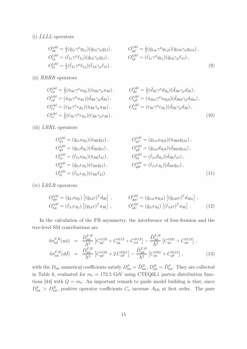
(i) LLLL operators

Oijklqq = 1

2(qLiγ

µqLj)(qLkγµqLl) , Oijklqq′ = 1

2(qLiaγ

µqLjb)(qLkbγµqLla) ,

Oijklℓq = (ℓLiγ

µℓLj)(qLkγµqLl) , Oijklℓq′ = (ℓLiγ

µqLj)(qLkγµℓLl) ,

Oijklℓℓ = 1

2(ℓLiγ

µℓLj)(ℓLkγµℓLl) . (9)

(ii) RRRR operators

Oijkluu = 1

2(uRiγ

µuRj)(uRkγµuRl) , Oijkldd = 1

2(dRiγ

µdRj)(dRkγµdRl) ,

Oijklud = (uRiγ

µuRj)(dRkγµdRl) , Oijklud′ = (uRiaγ

µuRjb)(dRkbγµdRla) ,

Oijkleu = (eRiγ

µeRj)(uRkγµuRl) , Oijkled = (eRiγ

µeRj)(dRkγµdRl) ,

Oijklee = 1

2(eRiγ

µeRj)(eRkγµeRl) . (10)

(iii) LRRL operators

Oijklqu = (qLiuRj)(uRkqLl) , Oijkl

qu′ = (qLiauRjb)(uRkbqLla) ,

Oijklqd = (qLidRj)(dRkqLl) , Oijkl

qd′ = (qLiadRjb)(dRkbqLla) ,

Oijklℓu = (ℓLiuRj)(uRkℓLl) , Oijkl

ℓd = (ℓLidRj)(dRkℓLl) ,

Oijklqe = (qLieRj)(eRkqLl) , Oijkl

qde = (ℓLieRj)(dRkqLl) ,

Oijklℓe = (ℓLieRj)(eRkℓLl) . (11)

(iv) LRLR operators

Oijklqqǫ = (qLiuRj)

[

(qLkǫ)TdRl

]

, Oijklqqǫ′ = (qLiauRjb)

[

(qLkbǫ)TdRla

]

,

Oijklℓqǫ = (ℓLieRj)

[

(qLkǫ)TuRl

]

, Oijklqℓǫ = (qLieRj)

[

(ℓLkǫ)TuRl

]

. (12)

In the calculation of the FB asymmetry, the interference of four-fermion and the

tree-level SM contributions are

δσF,Bint (uu) =

DF,Bint

Λ2

[

C1133

qq′ + C3113

qq + C3113

uu

]

− DF,Bint

Λ2

[

C1331

qu + C3113

qu

]

,

δσF,Bint (dd) =

DF,Bint

Λ2

[

C1133

qq′ + 2C3311

ud′

]

− DF,Bint

Λ2

[

C1331

qu + C3113

qd

]

, (13)

with the Dint numerical coefficients satisfy DFint = DB

int, DBint = DF

int. They are collected

in Table 6, evaluated for mt = 172.5 GeV using CTEQ6L1 parton distribution func-

tions [44] with Q = mt. An important remark to guide model building is that, since

DFint > DB

int, positive operator coefficients Cx increase AFB at first order. The pure

15

four-fermion contributions are

δσF,B4F (uu) =

DF,B1

Λ4

[

Π(C1133

qq + C3113

qq′ , C1133

qq′ + C3113

qq ) + Π(C1133

uu , C3113

uu )]

+DF,B

1

Λ4

[

Π(C1331

qu′ , C1331

qu ) + Π(C3113

qu′ , C3113

qu )]

+D2

Λ4Π(C3311

qu′ , C3311

qu )

−D4

Λ4

[

Π(C1133

qq + C3113

qq′ , C1331

qu′ , C1133

qq′ + C3113

qq , C1331

qu )

+Π(C3113

qu′ , C1133

uu , C3113

qu , C3113

uu )]

,

δσF,B4F (dd) = +

DF,B1

Λ4

[

Π(C1133

qq , C1133

qq′ ) + 4Π(C3311

ud , C3311

ud′ )]

+DF,B

1

Λ4

[

Π(C1331

qu′ , C1331

qu ) + Π(C3113

qd′ , C3113

qd ) + 1

2Π(C1331

qqǫ′ , C1331

qqǫ )]

+D2

Λ4Π(C3311

qqǫ , C3311

qqǫ′ ) +DF,B

3

Λ4ReΠ(C3311

qqǫ , C1331

qqǫ′ , C3311

qqǫ′ , C1331

qqǫ )

−D4

Λ4

[

Π(C1133

qq , C1331

qu′ , C1133

qq′ , C1331

qu ) + 2Π(C3113

qd′ , C3311

ud , C3113

qd , C3311

ud′ )]

,

(14)

with DF1= DB

1, DB

1= DF

1. We have used the functions

Π(x, y) = |x|2 + |y|2 + 2

3Re xy∗ ,

Π(x, y, u, v) = xy∗ + uv∗ +1

3xv∗ +

1

3uy∗ (15)

to write the expressions in a more compact form. The numerical coefficients are col-

lected in Table 6. Interference of four-fermion corrections and SM NLO corrections are

not considered.

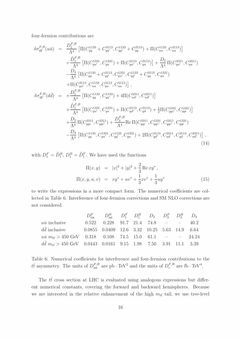
DFint DB

int DF1

DB1

D2 DF3

DB3

D4

uu inclusive 0.522 0.228 91.7 21.4 74.8 – – 40.2

dd inclusive 0.0855 0.0409 12.6 3.32 10.25 5.63 14.9 6.64

uu mtt > 450 GeV 0.318 0.108 74.5 15.0 61.1 – – 24.24

dd mtt > 450 GeV 0.0443 0.0161 9.15 1.98 7.50 3.91 11.1 3.39

Table 6: Numerical coefficients for interference and four-fermion contributions to the

tt asymmetry. The units of DF,Bint are pb · TeV2 and the units of DF,B

i are fb · TeV4.

The tt cross section at LHC is evaluated using analogous expressions but differ-

ent numerical constants, covering the forward and backward hemispheres. Because

we are interested in the relative enhancement of the high mtt tail, we use tree-level

16

calculations everywhere to be consistent. The tree-level SM cross section (including all

subprocesses) is 1.22 pb, and the four-fermion operator contributions to uu, dd → tt

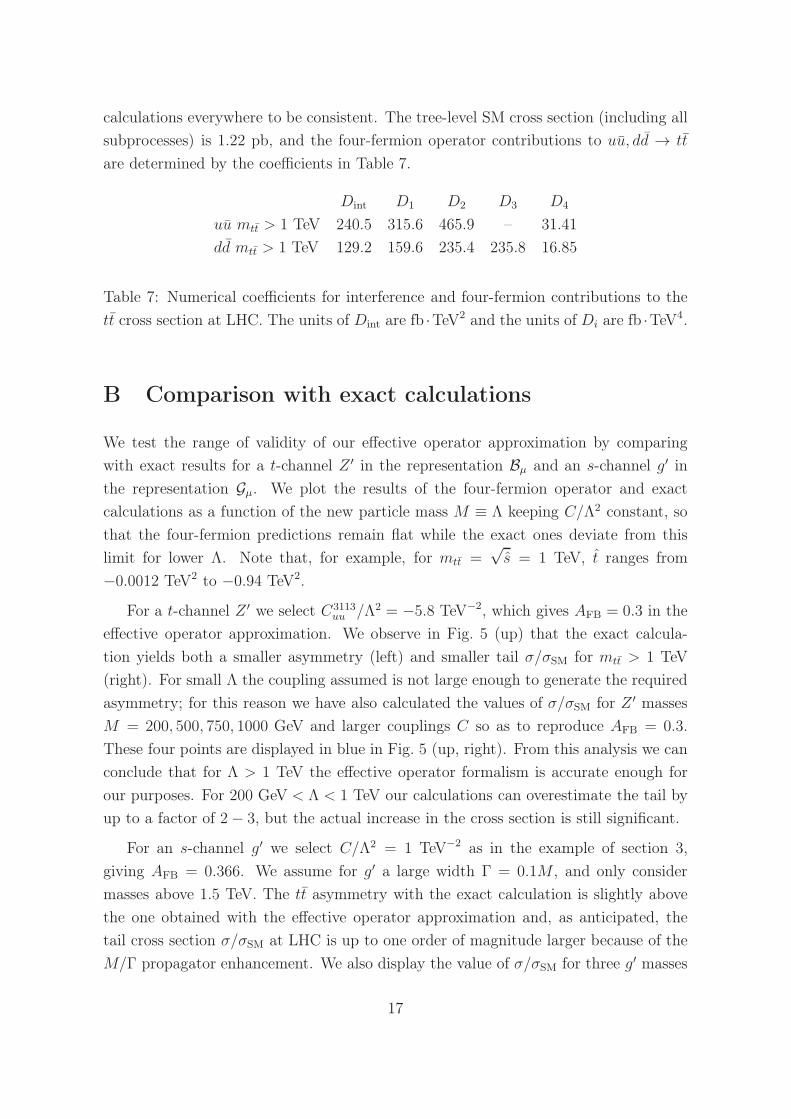
are determined by the coefficients in Table 7.

Dint D1 D2 D3 D4

uu mtt > 1 TeV 240.5 315.6 465.9 – 31.41

dd mtt > 1 TeV 129.2 159.6 235.4 235.8 16.85

Table 7: Numerical coefficients for interference and four-fermion contributions to the

tt cross section at LHC. The units of Dint are fb ·TeV2 and the units of Di are fb ·TeV4.

B Comparison with exact calculations

We test the range of validity of our effective operator approximation by comparing

with exact results for a t-channel Z ′ in the representation Bµ and an s-channel g′ in

the representation Gµ. We plot the results of the four-fermion operator and exact

calculations as a function of the new particle mass M ≡ Λ keeping C/Λ2 constant, so

that the four-fermion predictions remain flat while the exact ones deviate from this

limit for lower Λ. Note that, for example, for mtt =√s = 1 TeV, t ranges from

−0.0012 TeV2 to −0.94 TeV2.

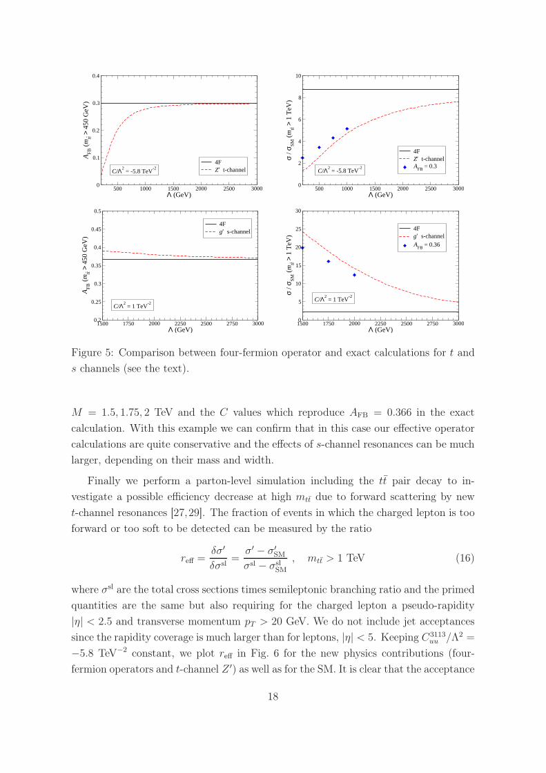
For a t-channel Z ′ we select C3113

uu /Λ2 = −5.8 TeV−2, which gives AFB = 0.3 in the

effective operator approximation. We observe in Fig. 5 (up) that the exact calcula-

tion yields both a smaller asymmetry (left) and smaller tail σ/σSM for mtt > 1 TeV

(right). For small Λ the coupling assumed is not large enough to generate the required

asymmetry; for this reason we have also calculated the values of σ/σSM for Z ′ masses

M = 200, 500, 750, 1000 GeV and larger couplings C so as to reproduce AFB = 0.3.

These four points are displayed in blue in Fig. 5 (up, right). From this analysis we can

conclude that for Λ > 1 TeV the effective operator formalism is accurate enough for

our purposes. For 200 GeV < Λ < 1 TeV our calculations can overestimate the tail by

up to a factor of 2− 3, but the actual increase in the cross section is still significant.

For an s-channel g′ we select C/Λ2 = 1 TeV−2 as in the example of section 3,

giving AFB = 0.366. We assume for g′ a large width Γ = 0.1M , and only consider

masses above 1.5 TeV. The tt asymmetry with the exact calculation is slightly above

the one obtained with the effective operator approximation and, as anticipated, the

tail cross section σ/σSM at LHC is up to one order of magnitude larger because of the

M/Γ propagator enhancement. We also display the value of σ/σSM for three g′ masses

17

500 1000 1500 2000 2500 3000Λ (GeV)

0

0.1

0.2

0.3

0.4

AFB

(m

tt > 4

50 G

eV)

4FZ′ t-channelC/Λ2

= -5.8 TeV-2

500 1000 1500 2000 2500 3000Λ (GeV)

0

2

4

6

8

10

σ / σ

SM (

mtt

> 1

TeV

)

4FZ′ t-channelA

FB = 0.3

C/Λ2 = -5.8 TeV

-2

1500 1750 2000 2250 2500 2750 3000Λ (GeV)

0.2

0.25

0.3

0.35

0.4

0.45

0.5

AFB

(m

tt > 4

50 G

eV)

4Fg′ s-channel

C/Λ2 = 1 TeV

-2

1500 1750 2000 2250 2500 2750 3000Λ (GeV)

0

5

10

15

20

25

30

σ / σ

SM (

mtt

> 1

TeV

)

4Fg′ s-channelA

FB = 0.36

C/Λ2 = 1 TeV

-2

Figure 5: Comparison between four-fermion operator and exact calculations for t and

s channels (see the text).

M = 1.5, 1.75, 2 TeV and the C values which reproduce AFB = 0.366 in the exact

calculation. With this example we can confirm that in this case our effective operator

calculations are quite conservative and the effects of s-channel resonances can be much

larger, depending on their mass and width.

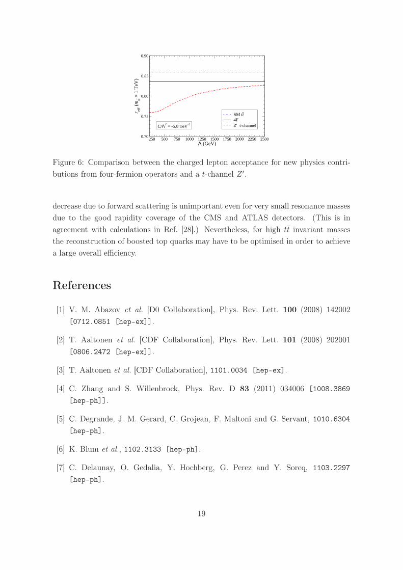
Finally we perform a parton-level simulation including the tt pair decay to in-

vestigate a possible efficiency decrease at high mtt due to forward scattering by new

t-channel resonances [27,29]. The fraction of events in which the charged lepton is too

forward or too soft to be detected can be measured by the ratio

reff =δσ′

δσsl=

σ′ − σ′SM

σsl − σslSM

, mtt > 1 TeV (16)

where σsl are the total cross sections times semileptonic branching ratio and the primed

quantities are the same but also requiring for the charged lepton a pseudo-rapidity

|η| < 2.5 and transverse momentum pT > 20 GeV. We do not include jet acceptances

since the rapidity coverage is much larger than for leptons, |η| < 5. Keeping C3113

uu /Λ2 =

−5.8 TeV−2 constant, we plot reff in Fig. 6 for the new physics contributions (four-

fermion operators and t-channel Z ′) as well as for the SM. It is clear that the acceptance

18

250 500 750 1000 1250 1500 1750 2000 2250 2500Λ (GeV)

0.70

0.75

0.80

0.85

0.90

r eff (

mtt >

1 T

eV)

SM tt4FZ′ t-channelC/Λ2

= -5.8 TeV-2

Figure 6: Comparison between the charged lepton acceptance for new physics contri-

butions from four-fermion operators and a t-channel Z ′.

decrease due to forward scattering is unimportant even for very small resonance masses

due to the good rapidity coverage of the CMS and ATLAS detectors. (This is in

agreement with calculations in Ref. [28].) Nevertheless, for high tt invariant masses

the reconstruction of boosted top quarks may have to be optimised in order to achieve

a large overall efficiency.

References

[1] V. M. Abazov et al. [D0 Collaboration], Phys. Rev. Lett. 100 (2008) 142002

[0712.0851 [hep-ex]].

[2] T. Aaltonen et al. [CDF Collaboration], Phys. Rev. Lett. 101 (2008) 202001

[0806.2472 [hep-ex]].

[3] T. Aaltonen et al. [CDF Collaboration], 1101.0034 [hep-ex].

[4] C. Zhang and S. Willenbrock, Phys. Rev. D 83 (2011) 034006 [1008.3869

[hep-ph]].

[5] C. Degrande, J. M. Gerard, C. Grojean, F. Maltoni and G. Servant, 1010.6304

[hep-ph].

[6] K. Blum et al., 1102.3133 [hep-ph].

[7] C. Delaunay, O. Gedalia, Y. Hochberg, G. Perez and Y. Soreq, 1103.2297

[hep-ph].

19

[8] I. Dorsner, S. Fajfer, J. F. Kamenik and N. Kosnik, Phys. Rev. D 81 (2010) 055009

[0912.0972 [hep-ph]].

[9] D. W. Jung, P. Ko and J. S. Lee, 1011.5976 [hep-ph].

[10] D. Choudhury, R. M. Godbole, S. D. Rindani and P. Saha, 1012.4750 [hep-ph].

[11] J. Cao, L. Wang, L. Wu and J. M. Yang, 1101.4456 [hep-ph].

[12] E. L. Berger, Q. H. Cao, C. R. Chen, C. S. Li and H. Zhang, 1101.5625 [hep-ph].

[13] Y. Bai, J. L. Hewett, J. Kaplan and T. G. Rizzo, JHEP 1103 (2011) 003

[1101.5203 [hep-ph]].

[14] B. Bhattacherjee, S. S. Biswal and D. Ghosh, 1102.0545 [hep-ph].

[15] K. M. Patel and P. Sharma, 1102.4736 [hep-ph].

[16] M. I. Gresham, I. W. Kim and K. M. Zurek, 1102.0018 [hep-ph].

[17] F. del Aguila, J. de Blas and M. Pérez-Victoria, JHEP 1009 (2010) 033

[1005.3998 [hep-ph]].

[18] J. A. Aguilar-Saavedra, Nucl. Phys. B 843 (2011) 638 [1008.3562 [hep-ph]].

[19] D. W. Jung, P. Ko, J. S. Lee and S. h. Nam, Phys. Lett. B 691 (2010) 238

[0912.1105 [hep-ph]].

[20] J. A. Aguilar-Saavedra, 1008.3225 [hep-ph].

[21] J. M. Campbell and R. K. Ellis, Phys. Rev. D 60 (1999) 113006

[hep-ph/9905386].

[22] J. Shu, T. M. P. Tait and K. Wang, Phys. Rev. D 81 (2010) 034012 [0911.3237

[hep-ph]].

[23] A. Arhrib, R. Benbrik and C. H. Chen, Phys. Rev. D 82 (2010) 034034 [0911.4875

[hep-ph]].

[24] Z. Ligeti, M. Schmaltz and G. M. Tavares, 1103.2757 [hep-ph].

[25] R. S. Chivukula, E. H. Simmons and C. P. Yuan, Phys. Rev. D 82 (2010) 094009

[1007.0260 [hep-ph]].

[26] J. A. Aguilar-Saavedra, Nucl. Phys. B 804 (2008) 160 [0803.3810 [hep-ph]].

20

[27] M. I. Gresham, I. W. Kim and K. M. Zurek, 1103.3501 [hep-ph].

[28] S. Jung, A. Pierce and J. D. Wells, 1103.4835 [hep-ph].

[29] S. Jung, H. Murayama, A. Pierce and J. D. Wells, Phys. Rev. D 81 (2010) 015004

[0907.4112 [hep-ph]].

[30] J. Cao, Z. Heng, L. Wu and J. M. Yang, Phys. Rev. D 81, 014016 (2010)

[0912.1447 [hep-ph]].

[31] K. Cheung, W. Y. Keung and T. C. Yuan, Phys. Lett. B 682 (2009) 287

[0908.2589 [hep-ph]].

[32] Q. H. Cao, D. McKeen, J. L. Rosner, G. Shaughnessy and C. E. M. Wagner, Phys.

Rev. D 81 (2010) 114004 [1003.3461 [hep-ph]].

[33] K. Cheung and T. C. Yuan, 1101.1445 [hep-ph].

[34] V. Barger, W. Y. Keung and C. T. Yu, 1102.0279 [hep-ph].

[35] B. Grinstein, A. L. Kagan, M. Trott and J. Zupan, 1102.3374 [hep-ph].

[36] P. Ferrario and G. Rodrigo, Phys. Rev. D 78 (2008) 094018 [0809.3354

[hep-ph]]; Phys. Rev. D 80 (2009) 051701 [0906.5541 [hep-ph]].

[37] P. H. Frampton, J. Shu and K. Wang, Phys. Lett. B 683 (2010) 294 [0911.2955

[hep-ph]].

[38] A. Djouadi, G. Moreau, F. Richard and R. K. Singh, Phys. Rev. D 82, 071702

(2010) [0906.0604 [hep-ph]].

[39] C. H. Chen, G. Cvetic and C. S. Kim, Phys. Lett. B 694 (2011) 393 [1009.4165

[hep-ph]].

[40] G. Burdman, L. de Lima and R. D. Matheus, Phys. Rev. D 83 (2011) 035012

[1011.6380 [hep-ph]].

[41] E. Alvarez, L. Da Rold and A. Szynkman, 1011.6557 [hep-ph].

[42] G. Isidori and J. F. Kamenik, 1103.0016 [hep-ph].

[43] CDF Collaboration, CDF note 10234.

[44] J. Pumplin, D. R. Stump, J. Huston, H. L. Lai, P. Nadolsky and W. K. Tung,

JHEP 0207 (2002) 012 [hep-ph/0201195].

21