arX

iv:h

ep-e

x/01

0201

0v1

7 F

eb 2

001

Fermilab-Conf-00-347-E

ELECTROWEAK AND B PHYSICS RESULTS FROMTHE FERMILAB TEVATRON COLLIDER

Kevin T. Pitts∗

University of Illinois, Department of Physics

1110 West Green Street, Urbana, IL 61801-3080, USA

E-mail: kpitts@uiuc.edu

Representing the CDF and DØ Collaborations

ABSTRACT

This writeup is an introduction to some of the experimental issues involvedin performing electroweak andb physics measurements at the FermilabTevatron. In the electroweak sector, we discussW andZ boson crosssection measurements as well as the measurement of the mass of theWboson. Forb physics, we discuss measurements ofB0/B0 mixing andCPviolation. This paper is geared towards nonexperts who are interested inunderstanding some of the issues and motivations for these measurementsand how the measurements are carried out.

∗Work supported by the Department of Energy, Contract DE-FG02-91ER40677.

1 Introduction

The Fermilab Tevatron collider is currently between data runs. The period from 1992-

1996, known as Tevatron Run 1, saw both the CDF and DØ experiments accumulate

approximately110 pb−1 of integrated luminosity. These data sets have yielded a large

number of results and publications on topics ranging from the discovery of the top

quark to precise measurements of the mass of theW boson; from measurements of

jet production at the highest energies ever observed to searches for physics beyond the

Standard Model.

This talk and subsequent paper focus on two aspects of the Tevatron program: elec-

troweak physics and the physics of hadrons containing the bottom quark. Each of these

topics is quite rich in its own right. It is not possible to do justice to either these topics

in the space provided.

Also, there are a large number of sources for summaries of recent results. For ex-

ample, many conference proceedings and summaries are easily accessible to determine

the most up-to-date measurements of the mass of theW boson. Instead of trying to

summarize a boat-load of Tevatron measurements here, I willattempt to describe a few

measurements in an introductory manner. The goal of this paper is to explain some

of the methods and considerations for these measurements. This paper therefore is

geared more towards students and non-experts. The goal hereis not to comprehensively

present the results, but to discuss how the results are obtained and what the important

elements are in these measurements.

After a brief discussion of the Tevatron collider and the twocollider experiments,

we will discuss electroweak andb physics at the Tevatron.

2 The Tevatron Collider

The Fermilab Tevatron collides protons(p) and antiprotons (p) at very high energy. In

past runs, thepp center of mass energy was√s = 1.8 TeV. It will be increased in

the future to2 TeV.∗ Until the Large Hadron Collider begins operation at CERN late

in this decade, the Tevatron will be the highest energy accelerator in the world. The

high energy, combined with a very high interaction rate, provides many opportunities

for unique and interesting measurements.∗For the upcoming Tevatron run, the center of mass energy willbe

√s = 1.96 TeV. Running the

machine at slightly below2 TeV drastically improves the reliability of the superconducting magnets.

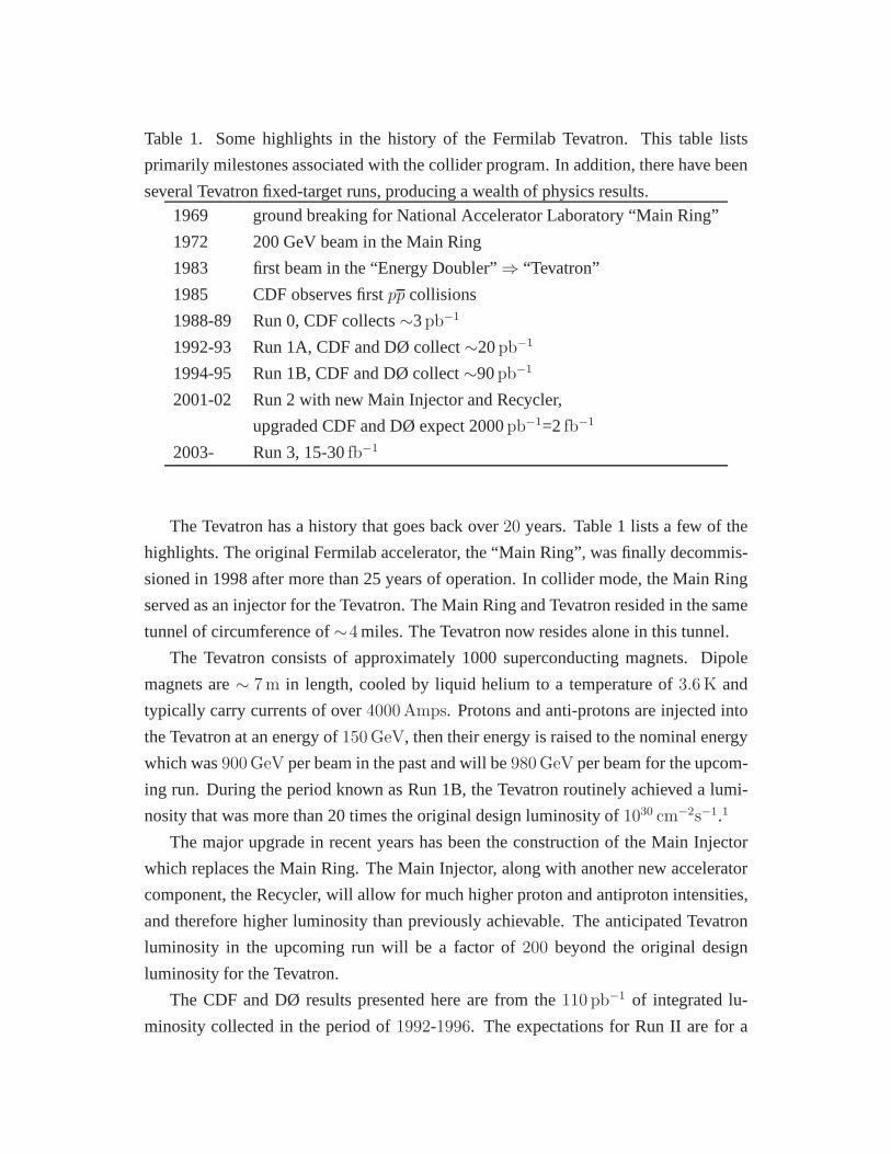
Table 1. Some highlights in the history of the Fermilab Tevatron. This table lists

primarily milestones associated with the collider program. In addition, there have been

several Tevatron fixed-target runs, producing a wealth of physics results.1969 ground breaking for National Accelerator Laboratory “Main Ring”

1972 200 GeV beam in the Main Ring

1983 first beam in the “Energy Doubler”⇒ “Tevatron”

1985 CDF observes firstpp collisions

1988-89 Run 0, CDF collects∼3pb−1

1992-93 Run 1A, CDF and DØ collect∼20pb−1

1994-95 Run 1B, CDF and DØ collect∼90pb−1

2001-02 Run 2 with new Main Injector and Recycler,

upgraded CDF and DØ expect 2000pb−1=2 fb−1

2003- Run 3, 15-30fb−1

The Tevatron has a history that goes back over20 years. Table 1 lists a few of the

highlights. The original Fermilab accelerator, the “Main Ring”, was finally decommis-

sioned in 1998 after more than 25 years of operation. In collider mode, the Main Ring

served as an injector for the Tevatron. The Main Ring and Tevatron resided in the same

tunnel of circumference of∼4 miles. The Tevatron now resides alone in this tunnel.

The Tevatron consists of approximately 1000 superconducting magnets. Dipole

magnets are∼ 7 m in length, cooled by liquid helium to a temperature of3.6 K and

typically carry currents of over4000 Amps. Protons and anti-protons are injected into

the Tevatron at an energy of150 GeV, then their energy is raised to the nominal energy

which was900 GeV per beam in the past and will be980 GeV per beam for the upcom-

ing run. During the period known as Run 1B, the Tevatron routinely achieved a lumi-

nosity that was more than 20 times the original design luminosity of 1030 cm−2s−1.1

The major upgrade in recent years has been the construction of the Main Injector

which replaces the Main Ring. The Main Injector, along with another new accelerator

component, the Recycler, will allow for much higher proton and antiproton intensities,

and therefore higher luminosity than previously achievable. The anticipated Tevatron

luminosity in the upcoming run will be a factor of200 beyond the original design

luminosity for the Tevatron.

The CDF and DØ results presented here are from the110 pb−1 of integrated lu-

minosity collected in the period of1992-1996. The expectations for Run II are for a

20-fold increase in the data sample by2003 (2 fb−1). Beyond Run II, the goal is to

increase the data sample by an additional factor of10 (15-30 fb−1) by the time that the

LHC begins producing results.

3 CDF and DØ

The CDF and DØ detectors are both axially symmetric detectors that cover about98%

of the full 4π solid angle around the proton-antiproton interaction point. The exper-

iments utilize similar strategies for measuring the interactions. Near the interaction

region, tracking systems accurately measure the trajectory of charged particles. Out-

side the tracking region, calorimeters surround the interaction region to measure the

energy of both the charged and neutral particles. Behind thecalorimeters are muon

detectors, that measure the deeply penetrating muons. Bothexperiments have fast trig-

ger and readout electronics to acquire data at high rates. Additional details about the

experiments can be found elsewhere.2,3

The strengths of the detectors are somewhat complementary to one another. The

DØ detector features a uranium liquid-argon calorimeter that has very good energy res-

olution for electron, photon and hadronic jet energy measurements. The CDF detector

features a1.4 T solenoid surrounding a silicon microvertex detector and gas-wire drift

chamber. These properties, combined with muon detectors and calorimeters, allow for

excellent muon and electron identification, as well as precise tracking and vertex detec-

tion forB physics.

4 Electroweak Results

Although many precise electroweak measurements have been performed at and above

theZ0 resonance at LEP and SLC, the Tevatron provides some unique and complemen-

tary measurements of electroweak phenomena. Some of these measurements include

W andZ production cross sections; gauge boson couplings (WW ,Wγ,WZ,Zγ,ZZ);

and properties of theW boson (mass, width, asymmetries).

For the most part, bothW andZ bosons are observed in hadron collisions through

leptonic decays to electrons and muons, such asW+ → e+νe andZ0 → µ+µ−. The

branching ratios for the leptonic decays of theW andZ are significantly smaller than

the branching ratios for hadronic decays. There are about 3.2 hadronicW decays for

everyW decay toe or µ and about 10 hadronicZ decays for everyZ decay toe+e−

or µ+µ−. Unfortunately, the dijet background from processes likeqg → qg andgg →qq/gg (in addition to higher order processes) totally swamp the signal fromZ0 → qq

andW+ → qq′.†

4.1 W andZ Production

The rate of production ofW andZ bosons is an interesting test of the theories of

both electroweak and strong interactions. The actual production rates are determined

by factors that include the gauge boson couplings to fermions (EW) and the parton

distribution functions and higher order corrections (QCD).

As an example analysis, we will discuss the measurement theZ production cross-

section from theZ0 → e+e− mode. The total number of events we observe will be:

N = Lint · σZ · Br(Z0 → e+e−) · ǫee (1)

whereL is the instantaneous luminosity,Lint =∫ Ldt is the integrated luminosity,

σZ = σ(pp → Z0X) is theZ boson production cross section,Br(Z0 → e+e−) is the

branching ratio forZ0 → e+e−, andǫee is the efficiency for observing this decay mode.

We have made the simplifying assumption that there are no background events in our

signal sample. Let’s take each term in turn:

• Lint =∫ Ldt: the integrated luminosity is measured in units ofcm−2 and is a

measure of the total number ofpp interactions. The instantaneous luminosity is

measured in units ofcm−2s−1. In this case, “integrated” refers to the total time

the detector was ready and able to measurepp interactions.‡

• σZ = σ(pp → Z0X): cross sections are measured in units ofcm2 and are often

quoted in units of “barns”, where1b = 10−24cm2. Typical electroweak cross

sections measured at the Tevatron are in nanobarns (nb = 10−9b) or picobarns

(pb = 10−12b). The total cross section forpp at the Tevatron is about70 mb =

70 × 10−3b. The cross section listed here is for any and all types ofZ boson

†There are special cases where hadronic decays of heavy gaugebosons have been observed: hadronic

W boson decays have been observed in top quark decays, and aZ0 → bb signal has been observed by

CDF. Also, both experiments have observedW andZ decays toτ leptons.‡We refer to the detector as “live” when it is ready and available to record data. If the detector is off

or busy processing another event, it is not available or ableto record additional data. This is known as

“dead-time”.

production. The “X” includes the remaining fragments of the initialp andp, in

addition to allowing for additional final state particles.

• Br(Z0 → e+e−): The branching ratio is the fraction ofZ0 bosons that decay to a

specific final state,e+e− in this example.§

• ǫee: Of theZ0 bosons that are produced and decay toe+e−, not all of them are

detected or accepted into the final event sample. Some of the events are beyond

the region of space the detector covers in addition to the fact that the detector is

not 100% efficient for detecting any signature.

Our ultimate goal is to extractσZ . Rearranging Equation 1, we have:

σZ =N

Lint · Br(Z0 → e+e−) · ǫee. (2)

From the data, we can count the number of signal events,N . To extract a cross section,

we need to know the terms in the denominator as well:

• The luminosity is measured by looking at the total rate forpp→ ppX in a specific

and well-defined detector region. This rate is measured as a function of time and

then integrated over the time the detector is live. The equation N = Lσ is used

again, in this case we already know the totalpp cross section(σ), so we can use

this equation to extractL. At e+e− machines, the measurement of the luminosity

is quite precise, with a relative error of1% or less. For hadron machines, that level

of precision is not possible. Typical relative uncertainties on the luminosity are

5-8%.4

• The branching ratio forZ0 → e+e− is measured quite precisely by the LEP and

SLC experiments. The world average value is used as an input here. The un-

certainty on that value is incorporated into the ultimate uncertainty on the cross

section.

• The efficiency for a final state like this is measured by a combination of simu-

lation and control data samples. Primarily, data samples are used that are well

understood. For example,Z0 decays (Z0 → e+e− andZ0 → µ+µ−) provide

an excellent sample of electrons and muons for detector calibration. The high

invariant mass of the lepton pair is a powerful handle to reject background.

§The branching ratio is the fraction of times that a particle will decay into a specific final state. More

concisely, the branching ratio isBr(Z0 → e+e−) = Γ(Z0 → e+e−)/Γ(Z0 → all), whereΓ(Z0 →e+e−) is the partial width forZ0 decaying toe+e− andΓ(Z0 → all) is the totalZ0 width.

1.75

2

2.25

2.5

2.75

σ(p —

p →

WX

→ e

,µν)

(nb

)

µ

e τ µ e

µ ee all

CDF Luminosity Normalization6% higher than D0 Normalization

stat+syst+lumi

D0/CDF : W

150

200

250

σ(p —

p →

ZX

→ e

e,µµX

) (p

b)

µ

e

µ

e

µ

eµ e

µ e all

D0/CDF : ZNNLO Theory(Van Neerven et al.)

92/93 94/95 88/89 92/93 94/95 all

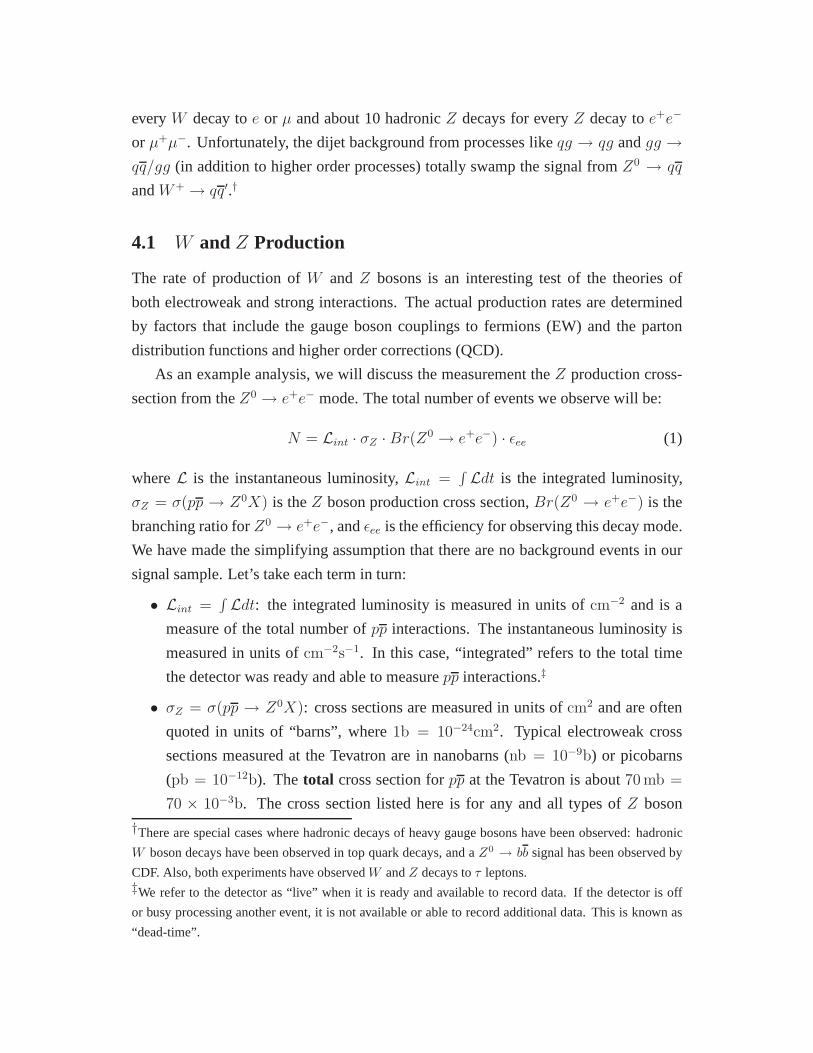
Fig. 1. Summary of DØ and CDFW andZ boson cross section measurements. The

solid bands indicate the theoretical prediction. The circular points are the DØ results;

the triangles are the CDF results. The two experiments use a different luminosity nor-

malization.

Putting all of these factors together, it is possible to measure the total cross sections

for pp → WX andpp → ZX. These measurements are performed independently in

both electron and muon modes. However, after the corrections for the efficiencies of

each mode, the measurements should (and do) yield consistent measured values for the

production cross section.

The results from DØ and CDF are represented in Fig. 1. The top plot is for W

production, the bottom plot forZ production. The shaded region is the theoretical

cross section. On both plots, the circular points are the DØ measurements, the triangles

the CDF measurements. Part of the difference in the results from the two experiments

arises from a different calculation ofLint. If a common calculation were used, the DØ

numbers would be6% larger than those presented. This shows that in fact the integrated

luminosity is the largest systematic uncertainty on the cross sections. Details of these

analyses may be found in the literature.5,6

4.2 R and theW Width

One way to make the measurement more sensitive to the electroweak aspects of theW

andZ production processes is to measure the cross section ratio.This ratio is often

referred to as “R”, and defined as:

R ≡ σ(W )

σ(Z)· Br(W → ℓν)

Br(Z → ℓℓ)

In taking the ratio of cross sections, the integrated luminosity (Lint) term and its

uncertainty cancel. Other experimental and theoretical uncertainties cancel as well,

making the measurement ofR a more stringent test of the Standard Model. As we can

see from Fig. 1, the ratio is about equal to10. This is confirmed by the results shown in

Table 2. The DØ result is for the electron final state7; the CDF result is for the electron

Table 2. Summary of Tevatron measurements ofR, whereR ≡ σ(W )σ(Z)

· Br(W→ℓν)Br(Z→ℓℓ)

.

measured value ofRDØ 10.43 ± 0.15(stat.) ± 0.20(syst.) ± 0.10(theory)

CDF 10.38 ± 0.14(stat.) ± 0.17(syst.)

and muon final states.8 For the CDF result, the theoretical uncertainty is contained in

the systematic uncertainty.

We can take this result one step further. The measured quantity isR. Theoretically,

the cross section ratioσ(W )/σ(Z) is calculated with good precision. This can be

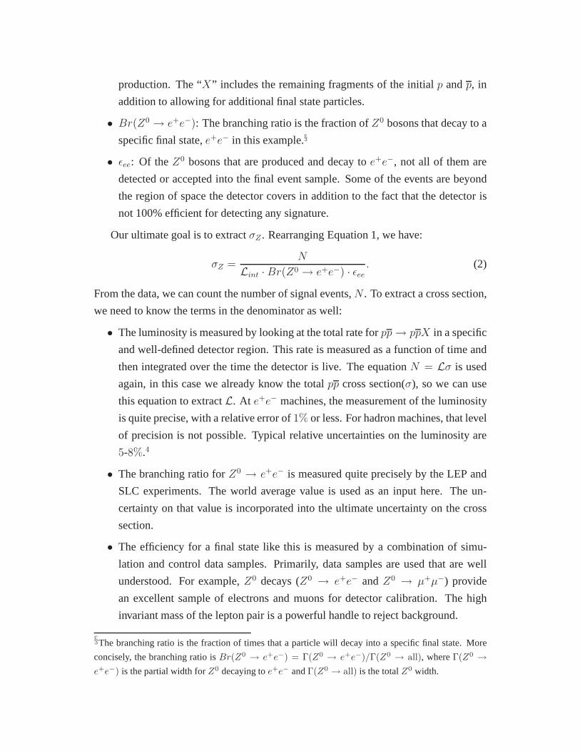
understood by noting that the primary production ofZ bosons at the Tevatron arise from

the reactions:uu→ Z0 anddd→ Z0, where the up and down quarks (and antiquarks)

can be valence or sea quarks in the proton. An example of valence-valence production

is shown in Fig. 2. ForW production, the primary contributions areud → W+ and

ud → W−. These reactions look quite similar to theZ production mechanisms where

a u quark is replaced with ad quark (or vice-versa). An example of valence-valence

W+ production is also shown in Fig. 2.

Although bothZ0 andW± are produced through quark-antiquark annihilation, the

dominant contribution is not from the valence-valence diagrams shown in Fig. 2. The

typical qq interaction energy for heavy boson production is the mass ofthe boson:√s ∼ MZ,W . Since the heavy boson massMZ,W ∼ 100 GeV = 0.1 TeV and thepp

center of mass energy is√s ∼2 TeV, the process requires theqq center of mass energy

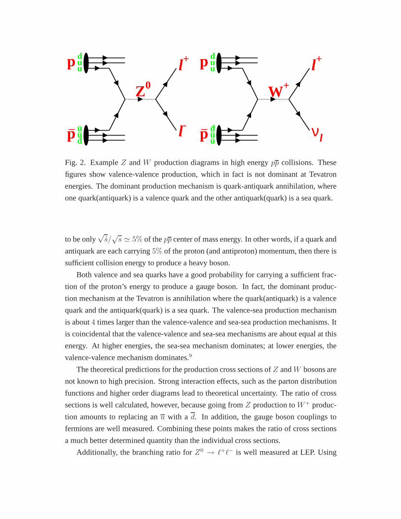
p_

p

Z0

l+

l-u_

u_

d_

uud

p_

p

W+

l+

νld_

u_

u_

uud

Fig. 2. ExampleZ andW production diagrams in high energypp collisions. These

figures show valence-valence production, which in fact is not dominant at Tevatron

energies. The dominant production mechanism is quark-antiquark annihilation, where

one quark(antiquark) is a valence quark and the other antiquark(quark) is a sea quark.

to be only√s/√s ≃ 5% of thepp center of mass energy. In other words, if a quark and

antiquark are each carrying5% of the proton (and antiproton) momentum, then there is

sufficient collision energy to produce a heavy boson.

Both valence and sea quarks have a good probability for carrying a sufficient frac-

tion of the proton’s energy to produce a gauge boson. In fact,the dominant produc-

tion mechanism at the Tevatron is annihilation where the quark(antiquark) is a valence

quark and the antiquark(quark) is a sea quark. The valence-sea production mechanism

is about4 times larger than the valence-valence and sea-sea production mechanisms. It

is coincidental that the valence-valence and sea-sea mechanisms are about equal at this

energy. At higher energies, the sea-sea mechanism dominates; at lower energies, the

valence-valence mechanism dominates.9

The theoretical predictions for the production cross sections ofZ andW bosons are

not known to high precision. Strong interaction effects, such as the parton distribution

functions and higher order diagrams lead to theoretical uncertainty. The ratio of cross

sections is well calculated, however, because going fromZ production toW+ produc-

tion amounts to replacing anu with a d. In addition, the gauge boson couplings to

fermions are well measured. Combining these points makes the ratio of cross sections

a much better determined quantity than the individual crosssections.

Additionally, the branching ratio forZ0 → ℓ+ℓ− is well measured at LEP. Using

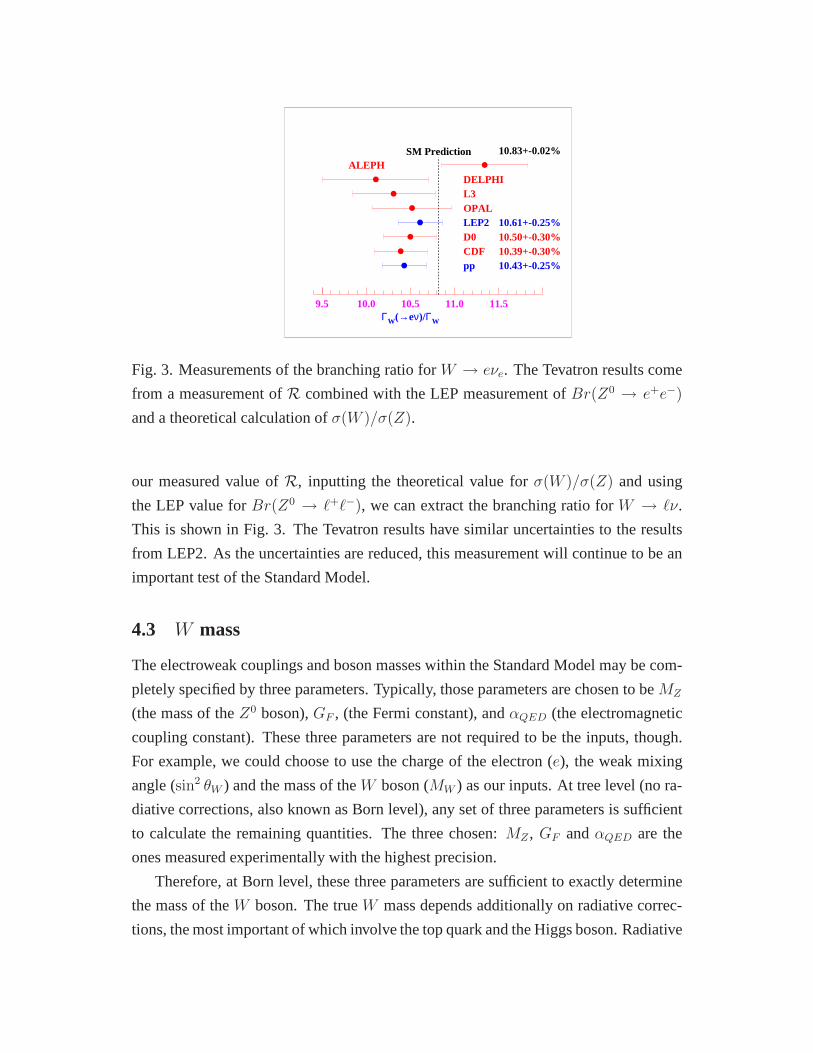
9.5 10.0 10.5 11.0 11.5ΓW(→eν)/ΓW

SM PredictionALEPH

DELPHIL3OPALLEP2 10.61+-0.25%D0 10.50+-0.30%CDF 10.39+-0.30%pp 10.43+-0.25%

10.83+-0.02%

Fig. 3. Measurements of the branching ratio forW → eνe. The Tevatron results come

from a measurement ofR combined with the LEP measurement ofBr(Z0 → e+e−)

and a theoretical calculation ofσ(W )/σ(Z).

our measured value ofR, inputting the theoretical value forσ(W )/σ(Z) and using

the LEP value forBr(Z0 → ℓ+ℓ−), we can extract the branching ratio forW → ℓν.

This is shown in Fig. 3. The Tevatron results have similar uncertainties to the results

from LEP2. As the uncertainties are reduced, this measurement will continue to be an

important test of the Standard Model.

4.3 W mass

The electroweak couplings and boson masses within the Standard Model may be com-

pletely specified by three parameters. Typically, those parameters are chosen to beMZ

(the mass of theZ0 boson),GF , (the Fermi constant), andαQED (the electromagnetic

coupling constant). These three parameters are not required to be the inputs, though.

For example, we could choose to use the charge of the electron(e), the weak mixing

angle (sin2 θW ) and the mass of theW boson (MW ) as our inputs. At tree level (no ra-

diative corrections, also known as Born level), any set of three parameters is sufficient

to calculate the remaining quantities. The three chosen:MZ , GF andαQED are the

ones measured experimentally with the highest precision.

Therefore, at Born level, these three parameters are sufficient to exactly determine

the mass of theW boson. The trueW mass depends additionally on radiative correc-

tions, the most important of which involve the top quark and the Higgs boson. Radiative

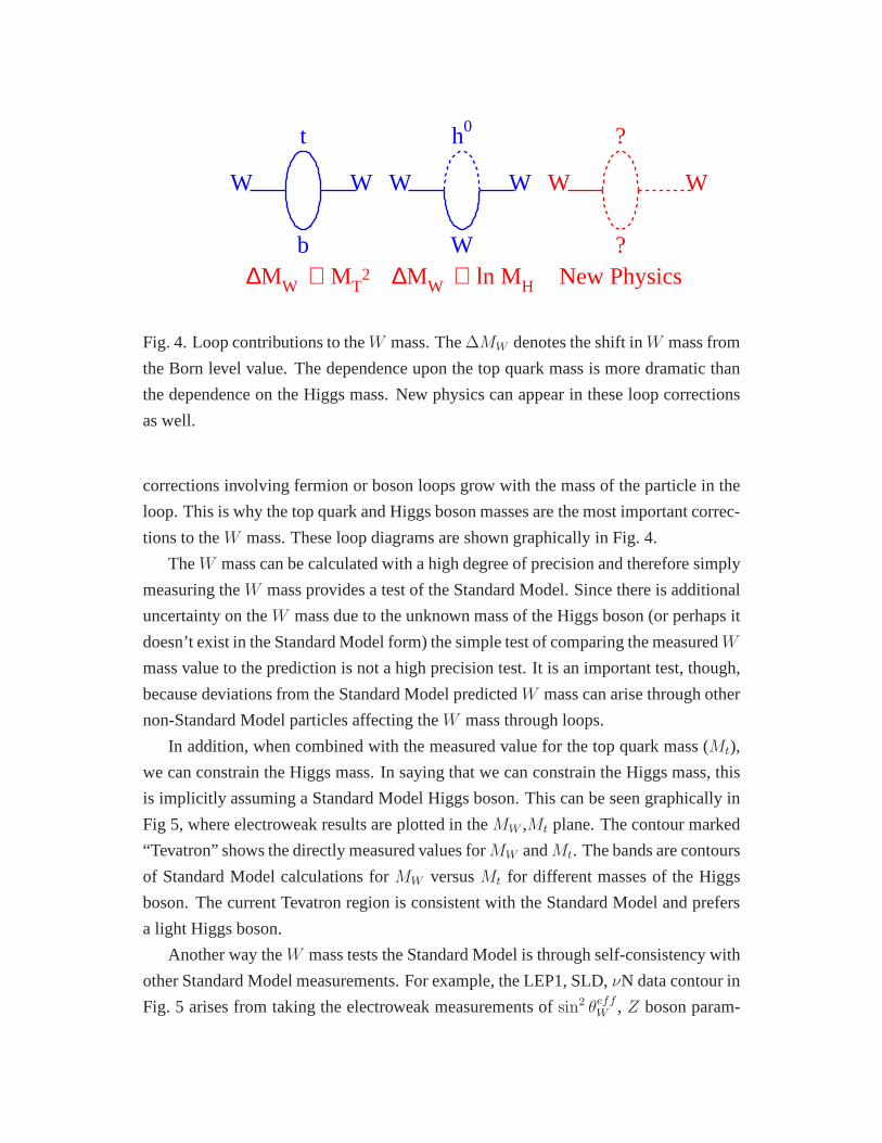
W W

t

b

W W

h0

W∆MW ∝ MT

2 ∆MW ∝ ln MH

W W

?

?New Physics

Fig. 4. Loop contributions to theW mass. The∆MW denotes the shift inW mass from

the Born level value. The dependence upon the top quark mass is more dramatic than

the dependence on the Higgs mass. New physics can appear in these loop corrections

as well.

corrections involving fermion or boson loops grow with the mass of the particle in the

loop. This is why the top quark and Higgs boson masses are the most important correc-

tions to theW mass. These loop diagrams are shown graphically in Fig. 4.

TheW mass can be calculated with a high degree of precision and therefore simply

measuring theW mass provides a test of the Standard Model. Since there is additional

uncertainty on theW mass due to the unknown mass of the Higgs boson (or perhaps it

doesn’t exist in the Standard Model form) the simple test of comparing the measuredW

mass value to the prediction is not a high precision test. It is an important test, though,

because deviations from the Standard Model predictedW mass can arise through other

non-Standard Model particles affecting theW mass through loops.

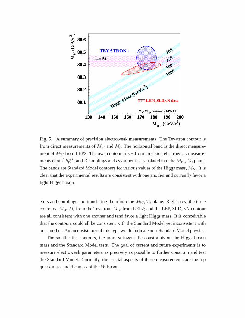
In addition, when combined with the measured value for the top quark mass (Mt),

we can constrain the Higgs mass. In saying that we can constrain the Higgs mass, this

is implicitly assuming a Standard Model Higgs boson. This can be seen graphically in

Fig 5, where electroweak results are plotted in theMW ,Mt plane. The contour marked

“Tevatron” shows the directly measured values forMW andMt. The bands are contours

of Standard Model calculations forMW versusMt for different masses of the Higgs

boson. The current Tevatron region is consistent with the Standard Model and prefers

a light Higgs boson.

Another way theW mass tests the Standard Model is through self-consistency with

other Standard Model measurements. For example, the LEP1, SLD, νN data contour in

Fig. 5 arises from taking the electroweak measurements ofsin2 θeffW , Z boson param-

80.1

80.2

80.3

80.4

80.5

80.6

130 140 150 160 170 180 190 200M top (GeV/c2)

MW

(G

eV/c

2 )

100

250

500

1000

Higgs Mass (GeV/c

2 )

TEVATRON

MW-M top contours : 68% CL

LEP2

LEP1,SLD,νN data

MW-M top contours : 68% CL

80.1

80.2

80.3

80.4

80.5

80.6

130 140 150 160 170 180 190 200

Fig. 5. A summary of precision electroweak measurements. The Tevatron contour is

from direct measurements ofMW andMt. The horizontal band is the direct measure-

ment ofMW from LEP2. The oval contour arises from precision electroweak measure-

ments ofsin2 θeffW , andZ couplings and asymmetries translated into theMW ,Mt plane.

The bands are Standard Model contours for various values of the Higgs mass,MH . It is

clear that the experimental results are consistent with oneanother and currently favor a

light Higgs boson.

eters and couplings and translating them into theMW ,Mt plane. Right now, the three

contours:MW ,Mt from the Tevatron;MW from LEP2; and the LEP, SLD,νN contour

are all consistent with one another and tend favor a light Higgs mass. It is conceivable

that the contours could all be consistent with the Standard Model yet inconsistent with

one another. An inconsistency of this type would indicate non-Standard Model physics.

The smaller the contours, the more stringent the constraints on the Higgs boson

mass and the Standard Model tests. The goal of current and future experiments is to

measure electroweak parameters as precisely as possible tofurther constrain and test

the Standard Model. Currently, the crucial aspects of thesemeasurements are the top

quark mass and the mass of theW boson.

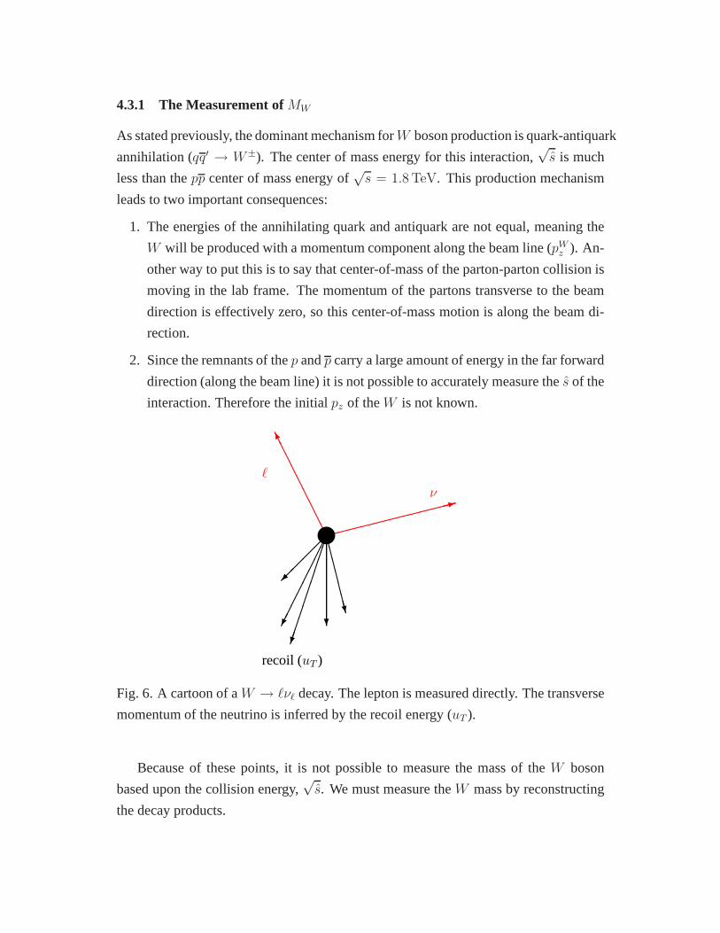
4.3.1 The Measurement ofMW

As stated previously, the dominant mechanism forW boson production is quark-antiquark

annihilation (qq′ → W±). The center of mass energy for this interaction,√s is much

less than thepp center of mass energy of√s = 1.8 TeV. This production mechanism

leads to two important consequences:

1. The energies of the annihilating quark and antiquark are not equal, meaning the

W will be produced with a momentum component along the beam line (pWz ). An-

other way to put this is to say that center-of-mass of the parton-parton collision is

moving in the lab frame. The momentum of the partons transverse to the beam

direction is effectively zero, so this center-of-mass motion is along the beam di-

rection.

2. Since the remnants of thep andp carry a large amount of energy in the far forward

direction (along the beam line) it is not possible to accurately measure thes of the

interaction. Therefore the initialpz of theW is not known.

✘✘✘✘✘✘✘✘✘✘✘✘✿ν

❆❆

❆❆

❆❆

❆❆

❆❑

ℓ

✂✂

✂✂

✂✂✂

✂✂✂✌

✁✁

✁✁

✁✁

✁✁☛

��

��✠

❄

❈❈❈❈❈❈❈❲

recoil (uT )

⑦

Fig. 6. A cartoon of aW → ℓνℓ decay. The lepton is measured directly. The transverse

momentum of the neutrino is inferred by the recoil energy (uT ).

Because of these points, it is not possible to measure the mass of theW boson

based upon the collision energy,√s. We must measure theW mass by reconstructing

the decay products.

0

50

100

150

200

250

300

60 70 80 90 100 110 120m(ee) (GeV)

num

ber

of e

vent

s

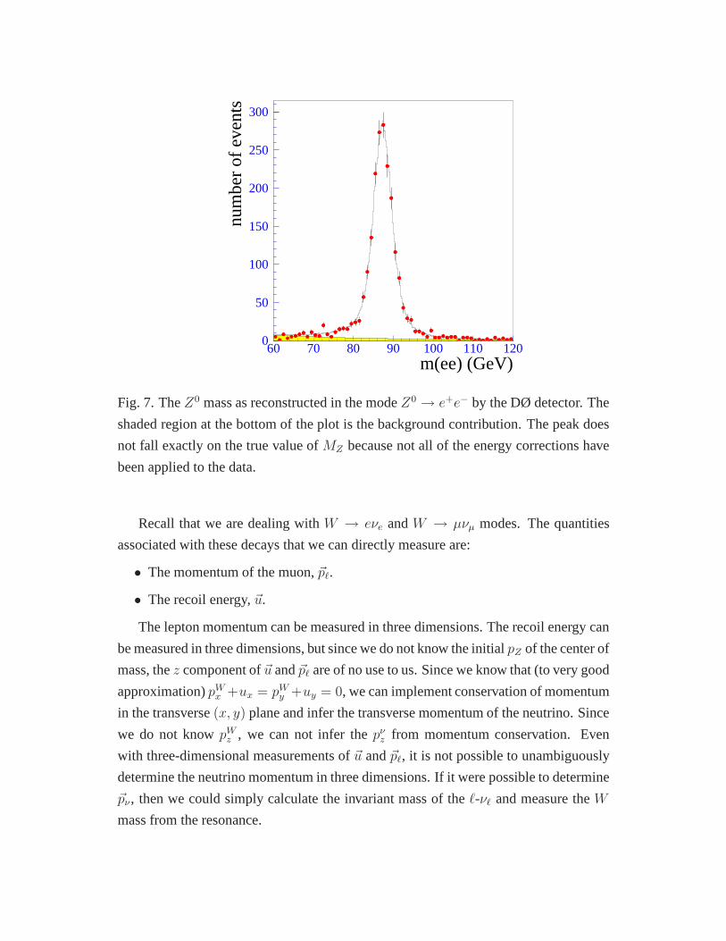
Fig. 7. TheZ0 mass as reconstructed in the modeZ0 → e+e− by the DØ detector. The

shaded region at the bottom of the plot is the background contribution. The peak does

not fall exactly on the true value ofMZ because not all of the energy corrections have

been applied to the data.

Recall that we are dealing withW → eνe andW → µνµ modes. The quantities

associated with these decays that we can directly measure are:

• The momentum of the muon,~pℓ.

• The recoil energy,~u.

The lepton momentum can be measured in three dimensions. Therecoil energy can

be measured in three dimensions, but since we do not know the initial pZ of the center of

mass, thez component of~u and~pℓ are of no use to us. Since we know that (to very good

approximation)pWx +ux = pW

y +uy = 0, we can implement conservation of momentum

in the transverse(x, y) plane and infer the transverse momentum of the neutrino. Since

we do not knowpWz , we can not infer thepν

z from momentum conservation. Even

with three-dimensional measurements of~u and~pℓ, it is not possible to unambiguously

determine the neutrino momentum in three dimensions. If it were possible to determine

~pν , then we could simply calculate the invariant mass of theℓ-νℓ and measure theW

mass from the resonance.

The case ofZ production as discussed above is quite similar toW production. The

difference, however, is that theZ can decay to two charged leptons that we can measure

in the detector. Figure 7 shows the reconstructedZ mass in the modeZ0 → e+e− from

the DØ detector. TheZ peak is clear and well-resolved, with small backgrounds.

In the case of theW mass, the information we have is momentum of the lepton~p ℓ

and transverse momentum of the neutrino,~p νT , which was inferred from the transverse

momentum of the lepton and the transverse recoil energy (~uT ).

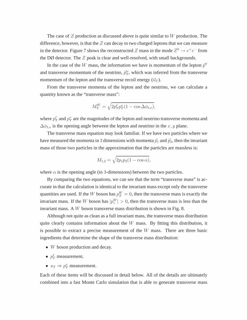
From the transverse momenta of the lepton and the neutrino, we can calculate a

quantity known as the “transverse mass”:

MWT =

√

2pℓTp

νT (1 − cos ∆φℓ,ν),

wherepℓT andpν

T are the magnitudes of the lepton and neutrino transverse momenta and

∆φℓ,ν is the opening angle between the lepton and neutrino in thex, y plane.

The transverse mass equation may look familiar. If we have two particles where we

have measured the momenta in3 dimensions with momenta~p1 and~p2, then the invariant

mass of those two particles in the approximation that the particles are massless is:

M1,2 =√

2p1p2(1 − cosα),

whereα is the opening angle (in3-dimensions) between the two particles.

By comparing the two equations, we can see that the term “transverse mass” is ac-

curate in that the calculation is identical to the invariantmass except only the transverse

quantities are used. If theW boson haspWZ = 0, then the transverse mass is exactly the

invariant mass. If theW boson has|pWz | > 0, then the transverse mass is less than the

invariant mass. AW boson transverse mass distribution is shown in Fig. 8.

Although not quite as clean as a full invariant mass, the transverse mass distribution

quite clearly contains information about theW mass. By fitting this distribution, it

is possible to extract a precise measurement of theW mass. There are three basic

ingredients that determine the shape of the transverse massdistribution:

• W boson production and decay.

• pℓT measurement.

• uT ⇒ pνT measurement.

Each of these items will be discussed in detail below. All of the details are ultimately

combined into a fast Monte Carlo simulation that is able to generate transverse mass

spectra corresponding to various values of theW mass. The measured transverse mass

distribution is then fit to the generated spectra and theW mass is extracted from this fit.

In the following subsections, we discuss each of the elements required for precise

W mass determination.

4.3.2 W boson production and decay

Modeling of theW boson production and decay includes the Breit-Wigner lineshape,

parton distribution functions, the momentum spectrum of the W boson, the recoil-

ing system and radiative corrections. The intrinsic width of the W boson is about

2.1 GeV/c2 which must be included in the fit. The parton distribution functions (PDF)

are representations of the distributions of valence quarks, sea quarks and gluons in the

proton. The probability for specific processes as a functionof s depend upon these

distributions. Related to the PDFs and the production diagrams is the momentum dis-

tribution of the producedW bosons. The model of the recoil system must be accurate.

Higher order QED diagrams, such asW → ℓνγ are also included in the modeling.

4.3.3 pℓT measurement

This aspect is quite crucial in theW mass determination. For muons, the transverse

momentum is measured by the track curvature in the magnetic field. For electrons, it

is more accurate to measure the energy (and infer the momentum) in the calorimeter

because the resolution is better and bremsstrahlung tends to bias the tracking measure-

ment of the curvature.

The energy scale is crucial. If we measure a muon with a transverse momentum of

30 GeV/c, is the true momentum30 GeV/c? Is it29.9 GeV/c? Is it30.1 GeV/c? Also,

the resolution is important to understand. For a measured momentum of30 GeV/c, we

also need to know the uncertainty on that value, because it will smear out the transverse

mass distribution. In reality, the resolution is a rather small effect, much smaller than

the overall momentum scale.

To set the momentum/energy scale, we use “calibration” samples. TheJ/ψ, Υ and

Z0 masses are all known very precisely based upon measurementsfrom other exper-

iments. We can measure these masses usingµ+µ− ande+e− final states to calibrate

our momentum scale. If a muon measured withpT = 29.9 GeV/c is truly a muon with

pT = 30.0 GeV/c, then we will measure an incorrectZ0 mass. This scale can be noted

and ultimately corrected.

0

500

1000

1500

2000

50 60 70 80 90 100 110 120

CDF(1B) PreliminaryW→eν

χ2/df = 82.6/70 (50 < MT < 120)

χ2/df = 32.4/35 (65 < MT < 100)

Mw = 80.473 +/- 0.065 (stat) GeV

KS(prob) = 16%

Fit region

Backgrounds

Transverse Mass (GeV)

# E

vent

s

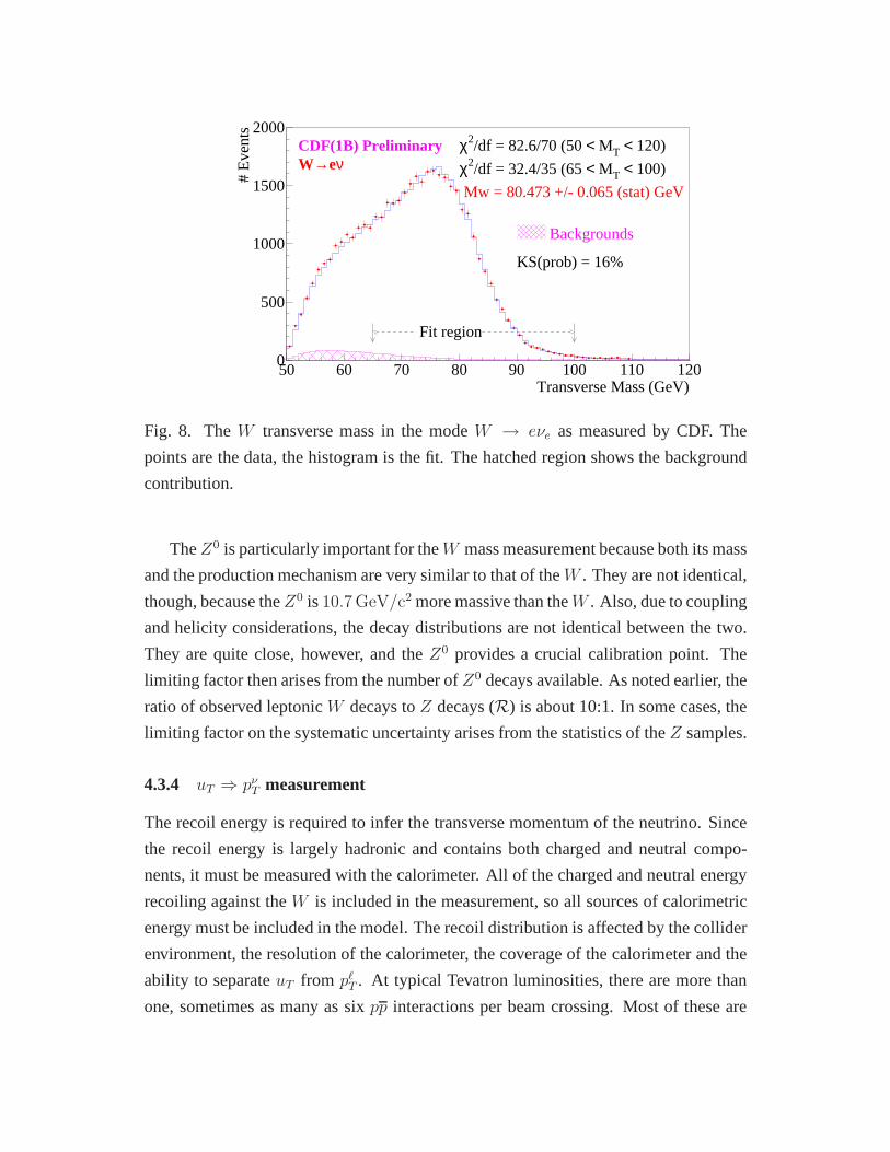
Fig. 8. TheW transverse mass in the modeW → eνe as measured by CDF. The

points are the data, the histogram is the fit. The hatched region shows the background

contribution.

TheZ0 is particularly important for theW mass measurement because both its mass

and the production mechanism are very similar to that of theW . They are not identical,

though, because theZ0 is10.7 GeV/c2 more massive than theW . Also, due to coupling

and helicity considerations, the decay distributions are not identical between the two.

They are quite close, however, and theZ0 provides a crucial calibration point. The

limiting factor then arises from the number ofZ0 decays available. As noted earlier, the

ratio of observed leptonicW decays toZ decays (R) is about 10:1. In some cases, the

limiting factor on the systematic uncertainty arises from the statistics of theZ samples.

4.3.4 uT ⇒ pνT measurement

The recoil energy is required to infer the transverse momentum of the neutrino. Since

the recoil energy is largely hadronic and contains both charged and neutral compo-

nents, it must be measured with the calorimeter. All of the charged and neutral energy

recoiling against theW is included in the measurement, so all sources of calorimetric

energy must be included in the model. The recoil distribution is affected by the collider

environment, the resolution of the calorimeter, the coverage of the calorimeter and the

ability to separateuT from pℓT . At typical Tevatron luminosities, there are more than

one, sometimes as many as sixpp interactions per beam crossing. Most of these are

inelastic events that have low transverse momentum. However, there is no way to di-

rectly separate out the contributions from other interactions from the contributions of

theW recoil. Instead, this must be modeled and the background level subtracted on an

average basis. Uncertainty in this background subtractionleads to uncertainty inMW .

The hadronic energy resolution of the calorimeter is much larger (i.e. worse) than

the resolution on the lepton energy. Therefore, the resolution on the neutrinopT is

determined by the hadronic energy resolution. The smaller this resolution, the less

smeared the transverse mass distribution.

The coverage of the calorimeter must be understood, also, because some of the

recoil can be carried away at very small angles to the beamline, where there is no

instrumentation.

Finally, the recoil measurement is a sum of all calorimeter energy except the energy

of the lepton. In the case of the muon channel, it is pretty straightforward to subtract

the contribution from the muon. For the electron, some of therecoil energy is included

in the electron energy cluster in the calorimeter simply because the recoil and elec-

tron energy “overlap”. This affects both the electron energy measurement and theuT

measurement and therefore we must correct for that effect.

4.3.5 W Mass Summary

Each of these pieces needs to be fully and accurately modeledin order to understand

how they effect the transverse mass distribution. There aremany important aspects to

this analysis, but the most important is the lepton energy scale. A great deal of work

has gone into calibrating, checking and understanding the lepton energy scale.

Details of the DØ and CDFW mass measurements may be found in Refs.10,11 For

a recent compilation of the world’sW mass measurements may be found in Ref.12

4.3.6 The Future

In addition to the Tevatron upgrades for Run II, the DØ and CDFcollaborations are

significantly upgrading their detectors.13,14 Figure 11 shows how the uncertainty on

theW mass has progressed over time. SinceN ∝ Lint, the horizontal axis, plotted

as√Lint is equivalent to

√NW , with NW being the number of identifiedW boson

decays. So far, the uncertainty on theW mass has fallen linearly with1/√NW . We

expect the statistical uncertainty to fall as1/√NW . The recent measurements ofMW

are not dominated by the statistical uncertainty, however.To maintain the1/√NW

79.5 79.7 79.9 80.1 80.3 80.5 80.7 80.9 81.1 81.3 81.5Mw (GeV)

UA2 (W → eν)

CDF(Run 1A, W → eν,µν)CDF(Run 1B, W → eν,µν)CDF combined

D0(Run 1A, W → eν)D0(Run 1B, W → eν)D0 combined

Hadron Collider Average

LEP II (ee → WW)

World Average

80.360 +/- 0.370

80.410 +/- 0.18080.470 +/- 0.08980.433 +/- 0.079

80.350 +/- 0.27080.498 +/- 0.09580.482 +/- 0.091

80.452 +/- 0.062

80.427 +/- 0.046

80.436 +/- 0.037

χ2/Nexp = 0.4/4

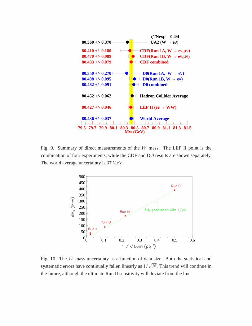
Fig. 9. Summary of direct measurements of theW mass. The LEP II point is the

combination of four experiments, while the CDF and DØ results are shown separately.

The world average uncertainty is37 MeV.

0

50

100

150

200

250

300

350

400

450

500

0 0.1 0.2 0.3 0.4 0.5 0.6

Fig. 10. TheW mass uncertainty as a function of data size. Both the statistical and

systematic errors have continually fallen linearly as1/√N . This trend will continue in

the future, although the ultimate Run II sensitivity will deviate from the line.

80.1

80.2

80.3

80.4

80.5

80.6

130 140 150 160 170 180 190 200M top (GeV/c2)

MW

(G

eV/c

2 )

100

250

500

1000

Higgs Mass (GeV/c

2 )

Tevatron2001-03

Per Expt

MW-M top contours : 68% CL

80.1

80.2

80.3

80.4

80.5

80.6

130 140 150 160 170 180 190 200

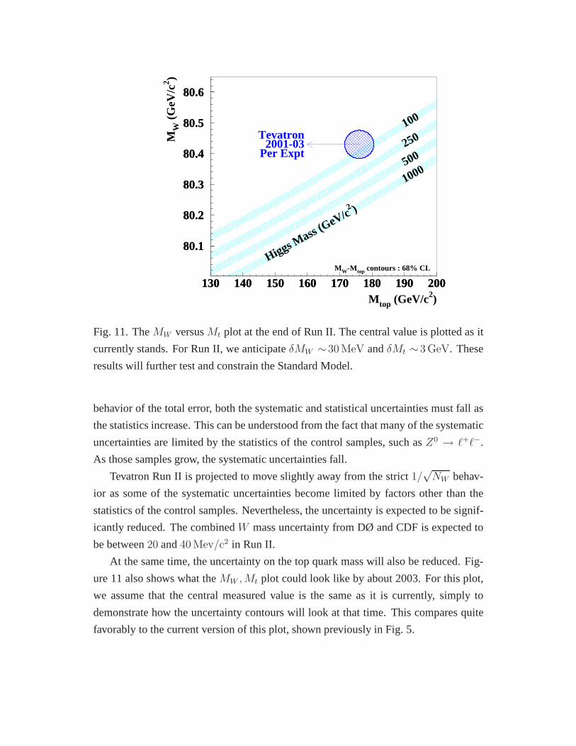
Fig. 11. TheMW versusMt plot at the end of Run II. The central value is plotted as it

currently stands. For Run II, we anticipateδMW ∼30 MeV andδMt ∼3 GeV. These

results will further test and constrain the Standard Model.

behavior of the total error, both the systematic and statistical uncertainties must fall as

the statistics increase. This can be understood from the fact that many of the systematic

uncertainties are limited by the statistics of the control samples, such asZ0 → ℓ+ℓ−.

As those samples grow, the systematic uncertainties fall.

Tevatron Run II is projected to move slightly away from the strict 1/√NW behav-

ior as some of the systematic uncertainties become limited by factors other than the

statistics of the control samples. Nevertheless, the uncertainty is expected to be signif-

icantly reduced. The combinedW mass uncertainty from DØ and CDF is expected to

be between20 and40 Mev/c2 in Run II.

At the same time, the uncertainty on the top quark mass will also be reduced. Fig-

ure 11 also shows what theMW ,Mt plot could look like by about 2003. For this plot,

we assume that the central measured value is the same as it is currently, simply to

demonstrate how the uncertainty contours will look at that time. This compares quite

favorably to the current version of this plot, shown previously in Fig. 5.

5 B Physics Results

Since the first observation of a violation of charge-conjugation parity (CP ) invariance

in the neutral kaon system in 1964,15 there has been an ongoing effort to further under-

stand the nature of the phenomenon. To date, violation ofCP symmetry has not been

directly observed anywhere other than the neutral kaon system. Within the framework

of the Standard Model,CP violation arises from a complex phase in the Cabibbo-

Kobayashi-Maskawa (CKM) quark mixing matrix,16 although the physics responsible

for the origin of this phase is not understood. The goal of current and future measure-

ments in theK andB meson systems is to continue to improve the constraints upon

the mixing matrix and further test the Standard Model. Inconsistencies would point

towards physics beyond the Standard Model.

In recent years, the importance and experimental advantages of theB system have

been emphasized.17 The long lifetime of theb quark, the large top quark mass and the

observation ofB0/B0 mixing with a long oscillation time all conspire to make theB

system fruitful in the study of the CKM matrix. Threee+e− B-factories running on

theΥ(4s) resonance in addition to experiments at HERA and the Tevatron indicate the

current level of interest and knowledge to be gained by detailed study of theB hadron

decays.

This section is an introduction toCP violation in theB system, with a focus on ex-

perimental issues. After a some notational definitions, I will give a brief overview of the

CKM matrix andB0/B0 mixing. Following that, I will discuss experimental elements

of flavor tagging, which is a crucial component in mixing andCP asymmetry measure-

ments. Our discussion ofCP violation in theB system will be presented in the frame-

work of the specific example of the measurement ofsin 2β usingB0/B0 → J/ψK0S

decays by the CDF Collaboration. Finally, I will briefly survey future measurements.

5.1 Notation

There are enoughB’s andb’s associated with this topic that it is worthwhile to specif-

ically spell out our notation. First of all, we will refer to bottom (antibottom) quarks

using small letters:b (b). When we are referring to generic hadrons containing a bottom

quark (e.g. |bq >, whereq is any quark type), we will use a capitalB with no specific

subscripts or superscripts.

In the cases where we are referring to specific bottom mesons or baryons, we will

us the notation listed in Table 3. NeutralB mesons follow the convention of the neutral

kaon system, whereK0 = |sd > andK0 = |sd >.

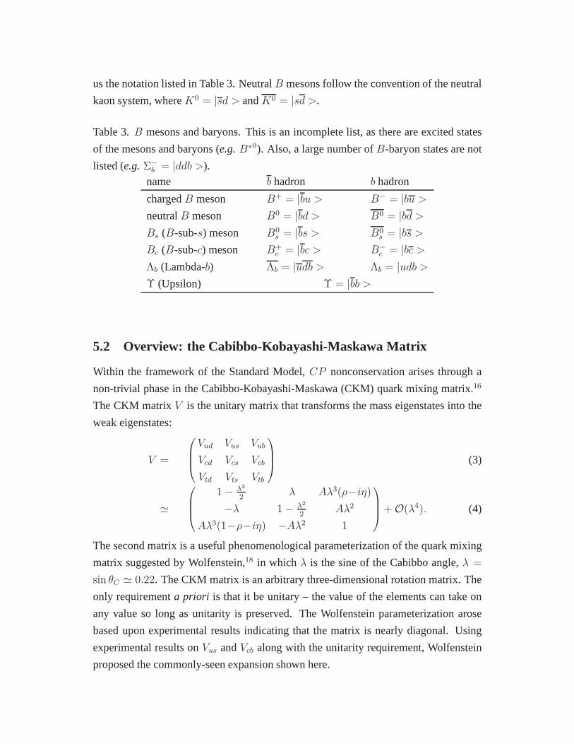
Table 3.B mesons and baryons. This is an incomplete list, as there are excited states

of the mesons and baryons (e.g. B∗0). Also, a large number ofB-baryon states are not

listed (e.g. Σ−b = |ddb >).

name b hadron b hadron

chargedB meson B+ = |bu > B− = |bu >neutralB meson B0 = |bd > B0 = |bd >Bs (B-sub-s) meson B0

s = |bs > B0s = |bs >

Bc (B-sub-c) meson B+c = |bc > B−

c = |bc >Λb (Lambda-b) Λb = |udb > Λb = |udb >Υ (Upsilon) Υ = |bb >

5.2 Overview: the Cabibbo-Kobayashi-Maskawa Matrix

Within the framework of the Standard Model,CP nonconservation arises through a

non-trivial phase in the Cabibbo-Kobayashi-Maskawa (CKM)quark mixing matrix.16

The CKM matrixV is the unitary matrix that transforms the mass eigenstates into the

weak eigenstates:

V =

Vud Vus Vub

Vcd Vcs Vcb

Vtd Vts Vtb

(3)

≃

1 − λ2

2λ Aλ3(ρ−iη)

−λ 1 − λ2

2Aλ2

Aλ3(1−ρ−iη) −Aλ2 1

+ O(λ4). (4)

The second matrix is a useful phenomenological parameterization of the quark mixing

matrix suggested by Wolfenstein,18 in which λ is the sine of the Cabibbo angle,λ =

sin θC ≃ 0.22. The CKM matrix is an arbitrary three-dimensional rotationmatrix. The

only requirementa priori is that it be unitary – the value of the elements can take on

any value so long as unitarity is preserved. The Wolfensteinparameterization arose

based upon experimental results indicating that the matrixis nearly diagonal. Using

experimental results onVus andVcb along with the unitarity requirement, Wolfenstein

proposed the commonly-seen expansion shown here.

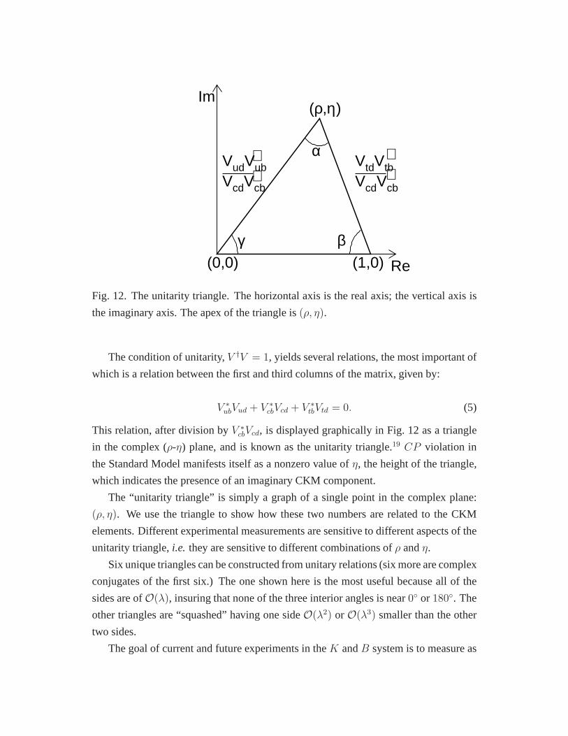
γ β

α

(ρ,η)

(0,0) (1,0)

VudVubVcdVcb

∗∗

VtdVtbVcdVcb

∗∗

Re

Im

Fig. 12. The unitarity triangle. The horizontal axis is the real axis; the vertical axis is

the imaginary axis. The apex of the triangle is(ρ, η).

The condition of unitarity,V †V = 1, yields several relations, the most important of

which is a relation between the first and third columns of the matrix, given by:

V ∗ubVud + V ∗

cbVcd + V ∗tbVtd = 0. (5)

This relation, after division byV ∗cbVcd, is displayed graphically in Fig. 12 as a triangle

in the complex (ρ-η) plane, and is known as the unitarity triangle.19 CP violation in

the Standard Model manifests itself as a nonzero value ofη, the height of the triangle,

which indicates the presence of an imaginary CKM component.

The “unitarity triangle” is simply a graph of a single point in the complex plane:

(ρ, η). We use the triangle to show how these two numbers are relatedto the CKM

elements. Different experimental measurements are sensitive to different aspects of the

unitarity triangle,i.e. they are sensitive to different combinations ofρ andη.

Six unique triangles can be constructed from unitary relations (six more are complex

conjugates of the first six.) The one shown here is the most useful because all of the

sides are ofO(λ), insuring that none of the three interior angles is near0◦ or 180◦. The

other triangles are “squashed” having one sideO(λ2) or O(λ3) smaller than the other

two sides.

The goal of current and future experiments in theK andB system is to measure as

many aspects of the triangle as possible in as many ways as possible. Inconsistencies

in these measurements will point to physics beyond the Standard Model and hopefully

give us some indication from where these “fundamental constants” arise.

Based upon current measurements in theK andB system, such asB0/B0 mixing,

K → π±ℓ∓ν, b → u decays andb → c decays, the CKM solution indicates that the

CP violating phase is large. The fact thatCP violation in theK system is small,

O(0.1%), arises from the fact that the magnitude of the matrix element Vtd is rather

small. An alternate solution would be if theCP violating phase were to be small and

the magnitude ofVtd larger. Direct measurements ofCP violation in theB system will

permit clear distinction between the two cases.20

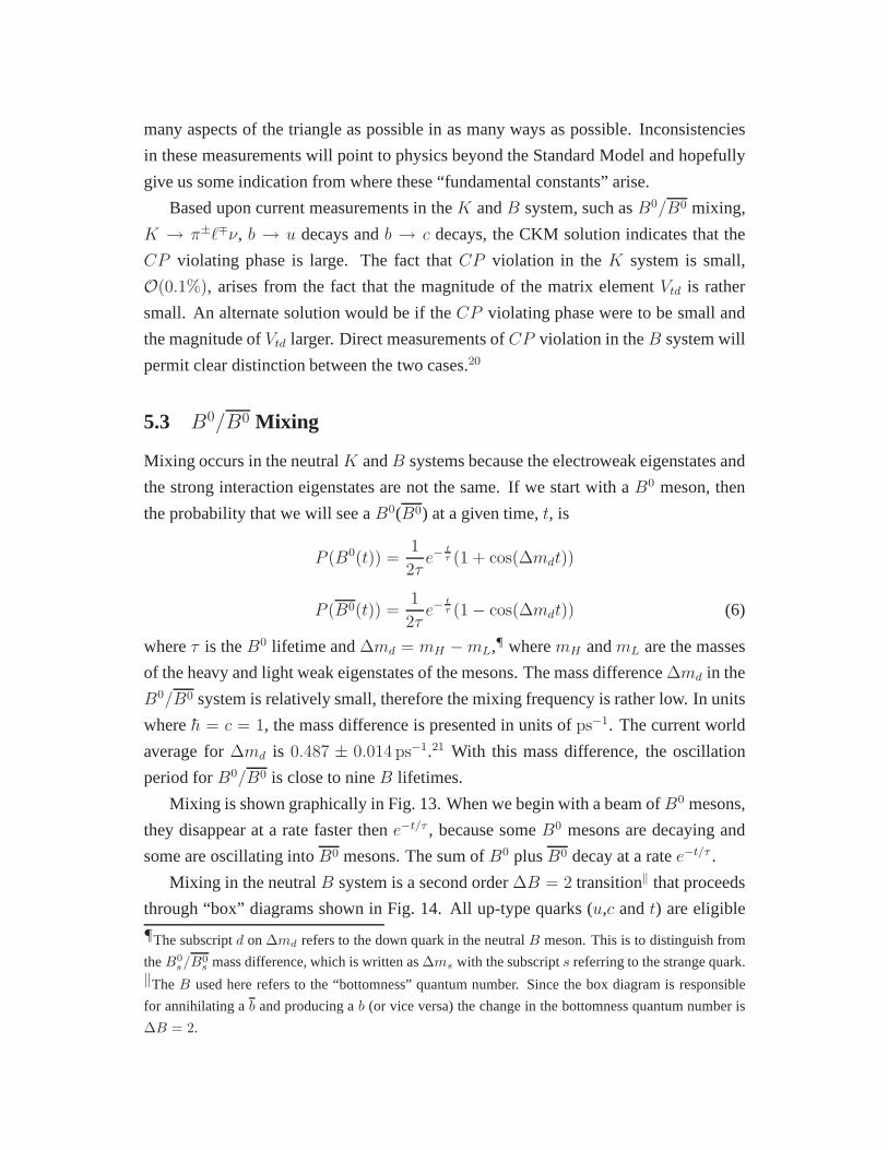
5.3 B0/B0 Mixing

Mixing occurs in the neutralK andB systems because the electroweak eigenstates and

the strong interaction eigenstates are not the same. If we start with aB0 meson, then

the probability that we will see aB0(B0) at a given time,t, is

P (B0(t)) =1

2τe−

tτ (1 + cos(∆mdt))

P (B0(t)) =1

2τe−

tτ (1 − cos(∆mdt)) (6)

whereτ is theB0 lifetime and∆md = mH −mL,¶ wheremH andmL are the masses

of the heavy and light weak eigenstates of the mesons. The mass difference∆md in the

B0/B0 system is relatively small, therefore the mixing frequencyis rather low. In units

whereh = c = 1, the mass difference is presented in units ofps−1. The current world

average for∆md is 0.487 ± 0.014 ps−1.21 With this mass difference, the oscillation

period forB0/B0 is close to nineB lifetimes.

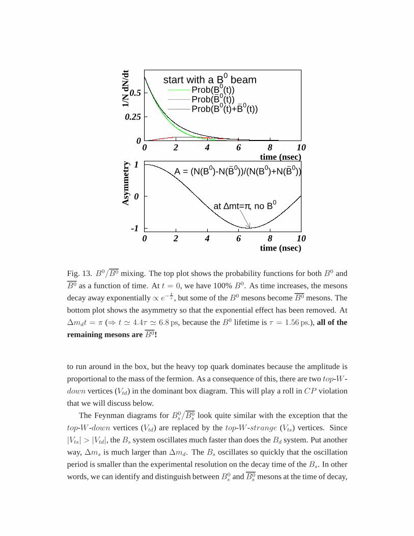
Mixing is shown graphically in Fig. 13. When we begin with a beam ofB0 mesons,

they disappear at a rate faster thene−t/τ , because someB0 mesons are decaying and

some are oscillating intoB0 mesons. The sum ofB0 plusB0 decay at a ratee−t/τ .

Mixing in the neutralB system is a second order∆B = 2 transition‖ that proceeds

through “box” diagrams shown in Fig. 14. All up-type quarks (u,c andt) are eligible

¶The subscriptd on∆md refers to the down quark in the neutralB meson. This is to distinguish from

theB0s/B0

smass difference, which is written as∆ms with the subscripts referring to the strange quark.

‖TheB used here refers to the “bottomness” quantum number. Since the box diagram is responsible

for annihilating ab and producing ab (or vice versa) the change in the bottomness quantum number is

∆B = 2.

time (nsec)

1/N

dN

/dt

start with a B0 beamProb(B0(t))Prob(B

– 0(t))Prob(B0(t)+B

– 0(t))

time (nsec)

Asy

mm

etry

A = (N(B0)-N(B– 0))/(N(B0)+N(B

– 0))

at ∆mt=π, no B0

0

0.25

0.5

0 2 4 6 8 10

-1

0

1

0 2 4 6 8 10

Fig. 13.B0/B0 mixing. The top plot shows the probability functions for bothB0 and

B0 as a function of time. Att = 0, we have 100%B0. As time increases, the mesons

decay away exponentially∝ e−tτ , but some of theB0 mesons becomeB0 mesons. The

bottom plot shows the asymmetry so that the exponential effect has been removed. At

∆mdt = π (⇒ t ≃ 4.4τ ≃ 6.8 ps, because theB0 lifetime is τ = 1.56 ps.), all of the

remaining mesons areB0!

to run around in the box, but the heavy top quark dominates because the amplitude is

proportional to the mass of the fermion. As a consequence of this, there are twotop-W -

down vertices (Vtd) in the dominant box diagram. This will play a roll inCP violation

that we will discuss below.

The Feynman diagrams forB0s/B

0s look quite similar with the exception that the

top-W -down vertices (Vtd) are replaced by thetop-W -strange (Vts) vertices. Since

|Vts| > |Vtd|, theBs system oscillates much faster than does theBd system. Put another

way, ∆ms is much larger than∆md. TheBs oscillates so quickly that the oscillation

period is smaller than the experimental resolution on the decay time of theBs. In other

words, we can identify and distinguish betweenB0s andB0

s mesons at the time of decay,

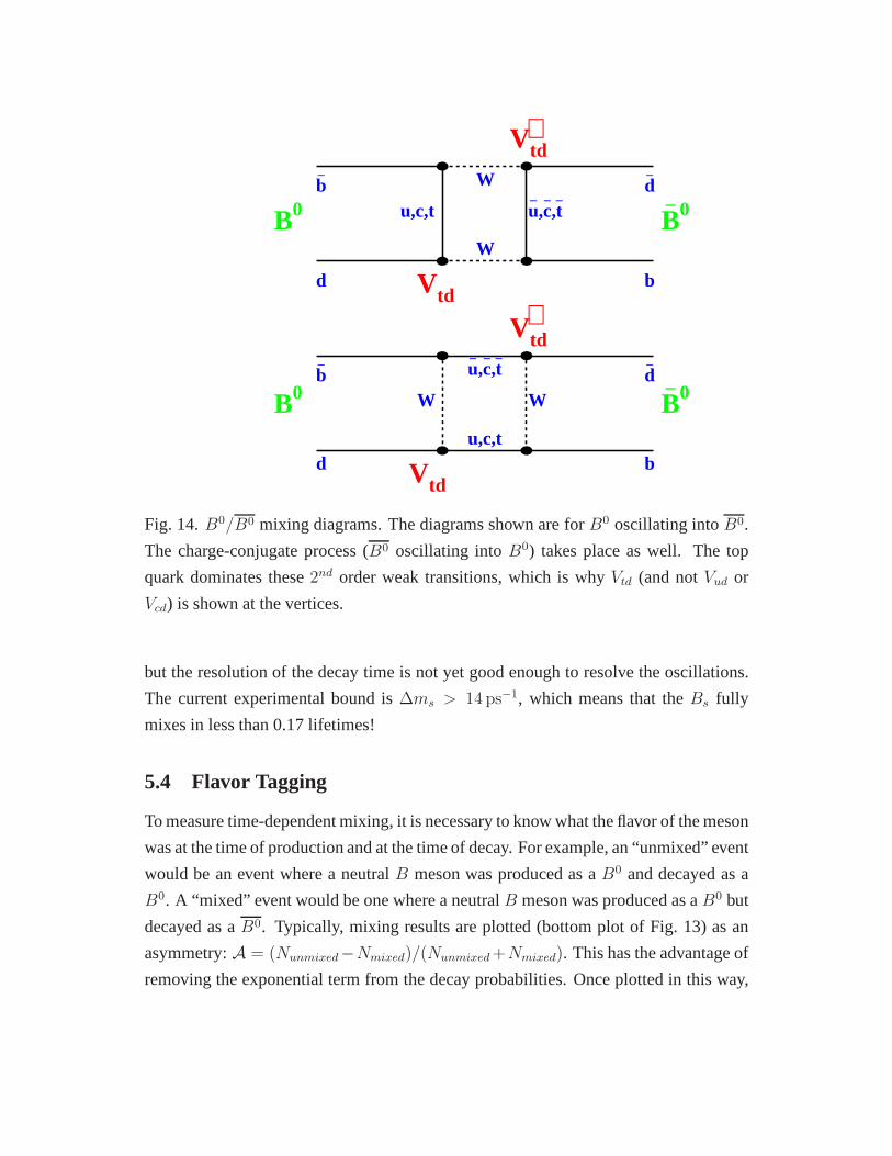
B0 B– 0

Vtd

Vtd∗

b–

d

d–

b

u,c,t u–,c–,t–

W

W

B0 B– 0

Vtd

Vtd∗

b–

d

d–

bu,c,t

u–,c–,t–

WW

Fig. 14.B0/B0 mixing diagrams. The diagrams shown are forB0 oscillating intoB0.

The charge-conjugate process (B0 oscillating intoB0) takes place as well. The top

quark dominates these2nd order weak transitions, which is whyVtd (and notVud or

Vcd) is shown at the vertices.

but the resolution of the decay time is not yet good enough to resolve the oscillations.

The current experimental bound is∆ms > 14 ps−1, which means that theBs fully

mixes in less than 0.17 lifetimes!

5.4 Flavor Tagging

To measure time-dependent mixing, it is necessary to know what the flavor of the meson

was at the time of production and at the time of decay. For example, an “unmixed” event

would be an event where a neutralB meson was produced as aB0 and decayed as a

B0. A “mixed” event would be one where a neutralB meson was produced as aB0 but

decayed as aB0. Typically, mixing results are plotted (bottom plot of Fig.13) as an

asymmetry:A = (Nunmixed−Nmixed)/(Nunmixed +Nmixed). This has the advantage of

removing the exponential term from the decay probabilities. Once plotted in this way,

the functional form of the mixing isA = cos ∆mdt.∗∗

Experimentally, the determination of the flavor of theB meson at the time of pro-

duction and/or the time of decay is referred to as “flavor tagging”. Flavor tagging is

an inexact science. TheB mesons have numerous decay modes, thanks in large part to

the large phase space for production of light hadrons in the dominantB → D → Xs

decay, whereD andXs represent generic charmed and strange hadrons respectively.

There is very low efficiency for fully reconstructingB states. Therefore more inclusive

techniques must be used to attempt to identify flavor.

Since flavor tagging is imprecise, it is crucial that we measure our success/failure

rate. There are two parameters required to describe flavor tagging. The first is known

as the tagging efficiency,ǫ, which is simply the fraction of events that are tagged. For

example, if we are only able to identify a lepton on10% of all of the events in our

sample, then the lepton tagging efficiency is10%. We can not distinguish aB0 from

aB0 in the other90% of the events because there was no lepton found to identify the

flavor.

The second parameter is associated with how often the identified flavor is correct.

A “mistag” is an event where the flavor was classified incorrectly. A mistag rate (w) of

40% is not unusual; while a mistag rate of 50% would mean that no flavor information

is available – equivalent to flipping a coin. Another way to classify the success rate is

through a variable called the “dilution” (D), defined as

D =Nright −Nwrong

Nright +Nwrong

= 1 − 2w (7)

whereNright(Nwrong) are the number of events tagged correctly (incorrectly). The term

is dubbed “dilution” because it dilutes the true asymmetry:

Aobserved = DAtrue (8)

whereAobserved is the experimentally measured asymmetry andAtrue is the measure-

ment of the real asymmetry we are trying to uncover.††

In the following subsections we discuss some commonly used flavor tagging tech-

niques. The methods outlined below are all utilized in mixing analyses. However, it∗∗Another common way to display mixing data is of the formA = Nmixed/(Nunmixed + Nmixed)

which then takes the functional formA = 1 − cos∆mdt.††The choice of the term “dilution” here is unfortunate, sincein this case a high dilution is good and a

low dilution is bad. The definition comes about because the factorD = 1 − 2w “dilutes” the measured

asymmetry. If our flavor tagging algorithm were perfect (no mistags) then we would haveD = 1, the

highest possible dilution.

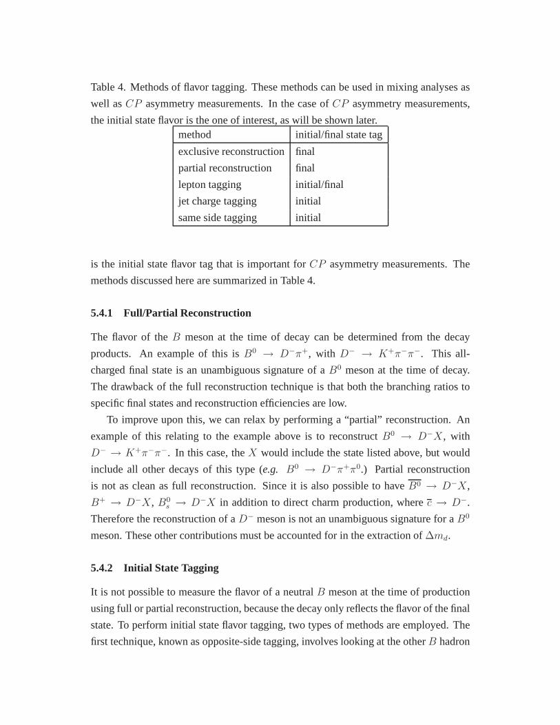
Table 4. Methods of flavor tagging. These methods can be used in mixing analyses as

well asCP asymmetry measurements. In the case ofCP asymmetry measurements,

the initial state flavor is the one of interest, as will be shown later.method initial/final state tag

exclusive reconstructionfinal

partial reconstruction final

lepton tagging initial/final

jet charge tagging initial

same side tagging initial

is the initial state flavor tag that is important forCP asymmetry measurements. The

methods discussed here are summarized in Table 4.

5.4.1 Full/Partial Reconstruction

The flavor of theB meson at the time of decay can be determined from the decay

products. An example of this isB0 → D−π+, with D− → K+π−π−. This all-

charged final state is an unambiguous signature of aB0 meson at the time of decay.

The drawback of the full reconstruction technique is that both the branching ratios to

specific final states and reconstruction efficiencies are low.

To improve upon this, we can relax by performing a “partial” reconstruction. An

example of this relating to the example above is to reconstruct B0 → D−X, with

D− → K+π−π−. In this case, theX would include the state listed above, but would

include all other decays of this type (e.g. B0 → D−π+π0.) Partial reconstruction

is not as clean as full reconstruction. Since it is also possible to haveB0 → D−X,

B+ → D−X, B0s → D−X in addition to direct charm production, wherec → D−.

Therefore the reconstruction of aD− meson is not an unambiguous signature for aB0

meson. These other contributions must be accounted for in the extraction of∆md.

5.4.2 Initial State Tagging

It is not possible to measure the flavor of a neutralB meson at the time of production

using full or partial reconstruction, because the decay only reflects the flavor of the final

state. To perform initial state flavor tagging, two types of methods are employed. The

first technique, known as opposite-side tagging, involves looking at the otherB hadron

µ+ µ-

π+

π-

same side π

2nd B

jet charge

lepton (e or µ)

Lxy

primary

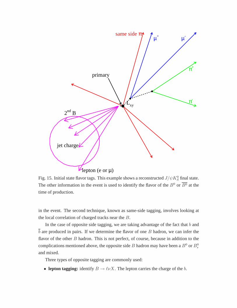
Fig. 15. Initial state flavor tags. This example shows a reconstructedJ/ψK0S final state.

The other information in the event is used to identify the flavor of theB0 orB0 at the

time of production.

in the event. The second technique, known as same-side tagging, involves looking at

the local correlation of charged tracks near theB.

In the case of opposite side tagging, we are taking advantageof the fact thatb and

b are produced in pairs. If we determine the flavor of oneB hadron, we can infer the

flavor of the otherB hadron. This is not perfect, of course, because in addition to the

complications mentioned above, the opposite sideB hadron may have been aB0 orB0s

and mixed.

Three types of opposite tagging are commonly used:

• lepton tagging: identifyB → ℓνX. The lepton carries the charge of theb.

b–

d

d–

u

π+

B0

fragmentation

b–

u

d–

d

B**+

π+

B0

via B**

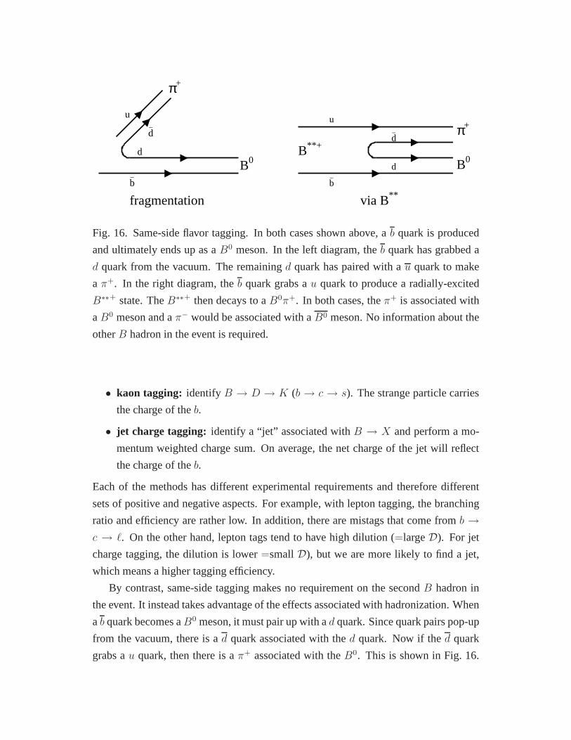
Fig. 16. Same-side flavor tagging. In both cases shown above,a b quark is produced

and ultimately ends up as aB0 meson. In the left diagram, theb quark has grabbed a

d quark from the vacuum. The remainingd quark has paired with au quark to make

a π+. In the right diagram, theb quark grabs au quark to produce a radially-excited

B∗∗+ state. TheB∗∗+ then decays to aB0π+. In both cases, theπ+ is associated with

aB0 meson and aπ− would be associated with aB0 meson. No information about the

otherB hadron in the event is required.

• kaon tagging: identifyB → D → K (b → c → s). The strange particle carries

the charge of theb.

• jet charge tagging: identify a “jet” associated withB → X and perform a mo-

mentum weighted charge sum. On average, the net charge of thejet will reflect

the charge of theb.

Each of the methods has different experimental requirements and therefore different

sets of positive and negative aspects. For example, with lepton tagging, the branching

ratio and efficiency are rather low. In addition, there are mistags that come fromb →c → ℓ. On the other hand, lepton tags tend to have high dilution (=largeD). For jet

charge tagging, the dilution is lower=smallD), but we are more likely to find a jet,

which means a higher tagging efficiency.

By contrast, same-side tagging makes no requirement on the secondB hadron in

the event. It instead takes advantage of the effects associated with hadronization. When

ab quark becomes aB0 meson, it must pair up with ad quark. Since quark pairs pop-up

from the vacuum, there is ad quark associated with thed quark. Now if thed quark

grabs au quark, then there is aπ+ associated with theB0. This is shown in Fig. 16.

An alternative path to the same correlation is through the production of aB∗∗ state. In

either case, the correlation is:B0π+ andB0π−. In our example above, if thed grabs a

d quark, then we have aπ0, in which case the first-order correlation is lost.

The same-side technique has the advantage of not relying on the secondB hadron

in the event. The disadvantage is that, depending upon the hadronization process for a

given event, the measured correlation may be absent or may beof the wrong sign. For

example, the correlation would not be measurable if the mesons from the fragmentation

chain were neutral. If the up quark in Fig. 16 were replaced bya down quark, then the

associated meson would be aπ0. Likewise, wrong-sign correlations are present: if the

up quark in Fig. 16 were replaced with a strange quark, then aK∗0 would be produced,

with K∗0 → K−π+. If theK− is selected as the tagging track, then the wrong-sign is

measured. This type of mistag can be reduced through the use of particle identification

to separate charged kaons, pions and protons.

As will be seen below, initial state flavor tagging is a crucial aspect in measuring

CP asymmetries in theB system. In the analysis we will discuss here, three of the four

initial state tagging methods are used: lepton tagging, jet-charge tagging and same-side

tagging.

5.5 CP Violation Via Mixing

For Standard ModelCP violation to occur, we need an interference to expose the

complex CKM phase. TheCP violating phase inVtd can manifest itself through the

∆B = 2 box diagrams responsible forB0/B0 mixing. In the Standard Model, the

decay modeB0/B0 → J/ψK0S is expected to exhibit mixing inducedCP violation.

This final state can be accessed by bothB0 andB0. CP violation in this case would

manifest itself as:

dN

dt(B0 → J/ψK0

S) 6= dN

dt(B0 → J/ψK0

S) (9)

whereJ/ψ = |cc >, K0S = 1√

2(|ds > +|sd >) and the final state,J/ψK0

S is a CP

eigenstate:

CP |J/ψK0S >= −|J/ψK0

S > (10)

In the CKM framework,CP violation occurs in this mode because the mixed decay

and direct decay interfere with one another. This is shown inFig. 17. An initial stateB0

can decay directly toJ/ψK0S, or it can mix into aB0 and then decay toJ/ψK0

S. The

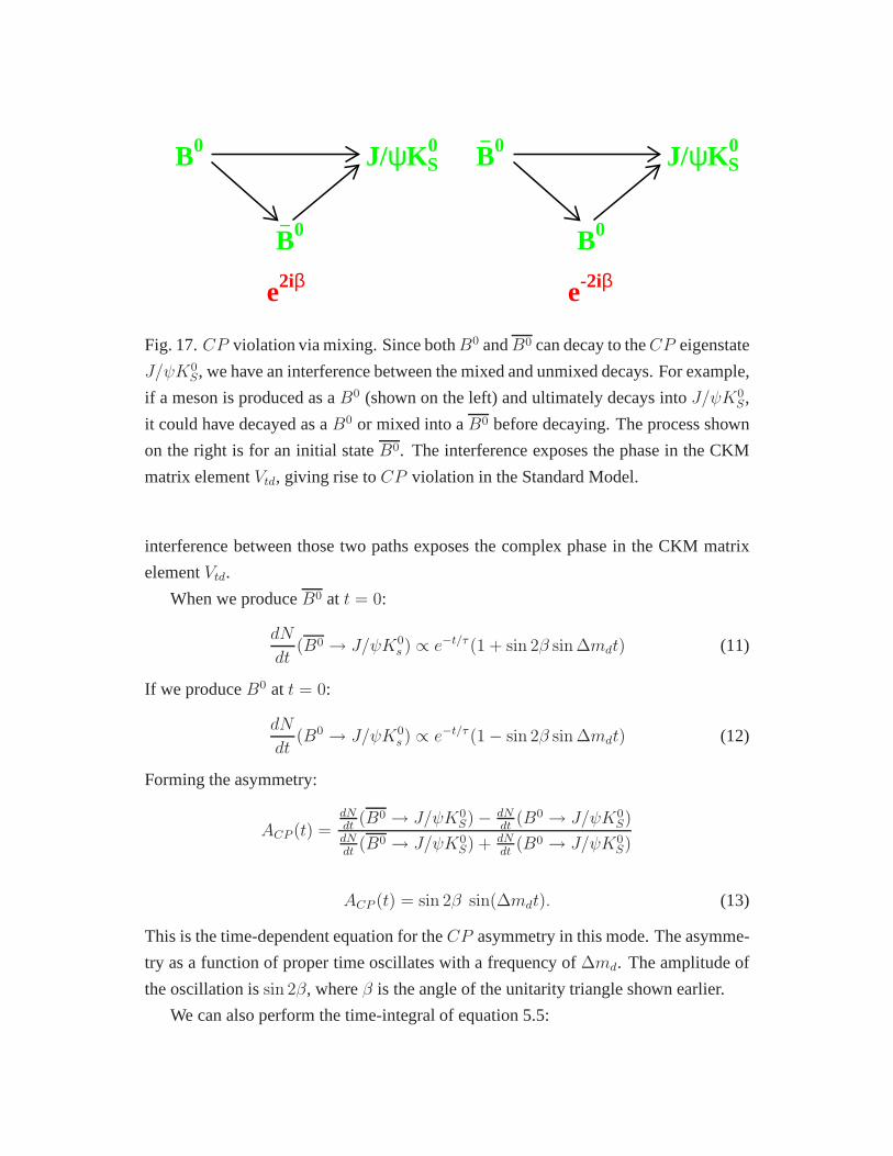
B0

B– 0

J/ψK0S

e2iβ

B– 0

B0

J/ψK0S

e-2iβ

Fig. 17.CP violation via mixing. Since bothB0 andB0 can decay to theCP eigenstate

J/ψK0S, we have an interference between the mixed and unmixed decays. For example,

if a meson is produced as aB0 (shown on the left) and ultimately decays intoJ/ψK0S,

it could have decayed as aB0 or mixed into aB0 before decaying. The process shown

on the right is for an initial stateB0. The interference exposes the phase in the CKM

matrix elementVtd, giving rise toCP violation in the Standard Model.

interference between those two paths exposes the complex phase in the CKM matrix

elementVtd.

When we produceB0 at t = 0:

dN

dt(B0 → J/ψK0

s ) ∝ e−t/τ (1 + sin 2β sin ∆mdt) (11)

If we produceB0 at t = 0:

dN

dt(B0 → J/ψK0

s ) ∝ e−t/τ (1 − sin 2β sin ∆mdt) (12)

Forming the asymmetry:

ACP (t) =dNdt

(B0 → J/ψK0S) − dN

dt(B0 → J/ψK0

S)dNdt

(B0 → J/ψK0S) + dN

dt(B0 → J/ψK0

S)

ACP (t) = sin 2β sin(∆mdt). (13)

This is the time-dependent equation for theCP asymmetry in this mode. The asymme-

try as a function of proper time oscillates with a frequency of ∆md. The amplitude of

the oscillation issin 2β, whereβ is the angle of the unitarity triangle shown earlier.

We can also perform the time-integral of equation 5.5:

ACP =

∫ dNdt

(B0 → ψK0

S)dt− ∫ dNdt

(B0 → ψK0S)dt

∫ dNdt

(B0 → ψK0

S)dt+∫ dN

dt(B0 → ψK0

S)dt(14)

ACP =N(B

0 → ψK0S) −N(B0 → ψK0

S)

N(B0 → ψK0

S) +N(B0 → ψK0S)

(15)

(16)

Integrating equations 12 an 11 and substituting them, we get:

ACP =∆mdτB

1 + (∆mdτB)2· sin 2β (17)

ACP ≃ 0.47 sin 2β (18)

This shows that we do not need to measure the proper time of theevents. Integrating

over all lifetimes still yields an asymmetry, although information is lost in going from

the time dependent to the time-integrated asymmetry. The above formalism is true

when theB0 andB0 are produced in an incoherent state, as they are in high energy

hadron collisions. At theΥ(4s), theB0 andB0 are produced in a coherent state and

the time-integrated asymmetry vanishes.22

5.6 Experimental Issues

The bottom line when it comes toCP violation in theB system is that you need to

tell the difference betweenB0 mesons andB0 mesons at the time of production. After

identifying a sample of signal events, flavor tagging is the most important aspect of

analyses ofCP violation.

In the case of theJ/ψK0S final state, we have no way of knowing whether the meson

was aB0 orB0 as it decayed, nor do we need to know. The difference we are attempting

to measure is the decay rate difference for mesons that wereproduced asB0 orB0. In

this case, we are tagging the flavor of theB meson when it was produced.

The analysis we are going to discuss here is a measurement of theCP asymmetry in

B0/B0 → J/ψK0S from the CDF experiment. Before discussing that measurement, we

begin with by presenting some of the unique aspects tob physics in the hadron collider

environment.

5.6.1 B Production and Reconstruction

First of all, thebb cross section is enormous,O(100µb), which means at typical operat-

ing luminosities, 1000bb pairs are produced every second! Thebb quarks are produced

by the strong interaction, which preserves “bottomness”, therefore they are always pro-

duced in pairs. The transverse momentum (pT ) spectrum for the producedB hadrons

is falling very rapidly, which means that most of theB hadrons have very low trans-

verse momentum. For the sample ofB → J/ψK0S decays we are discussing here, the

averagepT of theB meson is about10 GeV/c. The fact that theB hadrons have low

transverse momentum does not mean that they have low total momentum. Quite fre-

quently, theB mesons have very large longitudinal momentum (longitudinal being the

component along the beam axis.) TheseB hadrons are boosted along the beam axis

and are consequently outside the acceptance of the detector.

For bb production, likeW production discussed previously, the center of mass of

the parton-parton collision is not at rest in the lab frame. Even in the cases where one

B hadron is reconstructed (fully or partially) within the detector, the secondB hadron

may be outside the detector acceptance.

To identify theB mesons, we must first trigger the detector readout. Even though

thebb production rate is large, it is about 1000 times below the generic inelastic scat-

tering rate. In the trigger, we attempt to identify leptons:electrons and muons. In this

analysis, we look for two muons, indicating that we may have had aJ/ψ → µ+µ−

decay.∗

Once we have the data on tape, we can attempt to fully reconstruct theB0/B0 →J/ψK0

S final state. The event topology that we are describing here can be seen in

Fig. 15. To reconstructB → J/ψK0S, we again look forJ/ψ → µ+µ−, this time

with criteria more stringent than those imposed by the trigger. Once we find a dimuon

pair with invariant mass consistent with theJ/ψ mass, we then look for the decay

K0S → π+π−. At this point, we require the dipion mass be consistent withaK0

S mass,

and we also take advantage of the fact that theK0S lives a macroscopic distance in

the lab frame. Once we have both aJ/ψ andK0S candidate, we put them all together

to see if they were consistent with the decayB0/B0 → J/ψK0S. For example, the

momentum of theK0S must point back to theB decay vertex, and theB must point

∗It is difficult to trigger on the decayJ/ψ → e+e− at a hadron collider. The distinct aspect of electrons

is their energy deposition profile in the calorimeter. For low pT electrons fromJ/ψ decays (pT <

10 GeV/c), there is sufficient overlap from other particles to cause high trigger rates and low signal-to-

noise.

(Mµµππ-MB)/σM

even

ts

0

50

100

150

200

-20 -10 0 10 20

Fig. 18. B0/B0 → J/ψK0S event yield after the selection criteria discussed in the

text have been applied. The data is plotted in units of “normalized mass”:mnorm =

(Mfit −MB)/σfit, whereMfit andσfit are the four track fitted mass and uncertainty,

respectively, andMB is the world averageB0 mass. Signal events show up withMnorm

near zero, while combinatoric background shows up uniformly across the plot.

back to the primary (collision) vertex. After all of these selection criteria, we have a

sample of 400 signal events with a signal to noise of about 0.7-to-1, as shown in Fig 18.

5.6.2 Flavor Tagging and Asymmetry Measurement

Now that we have a sample of signal events (intermixed with background), we must

attempt to identify the flavor of theB0 orB0 at the time of production using the flavor

tagging techniques outlined above. For this analysis, we use three techniques: same-

side tagging, lepton tagging and jet charge tagging. The lepton and jet charge flavor tags

are looking at information from the otherB hadron in the event to infer the flavor of

theB we reconstructed. Table 5 summarizes the flavor tagging efficiency and dilution

for each of the algorithms.

Table 5. Summary of tagging algorithms performance. All numbers listed are in per-

cent. The efficiencies are obtained from theB → J/ψK0S sample. The dilution infor-

mation is derived from theB± → J/ψK± sample.

tag side tag type efficiency (ǫ) dilution (D) ǫD2

same-side same-side 73.6 ± 3.8 16.9 ± 2.2 2.1 ± 0.5

opposite side soft lepton 5.6 ± 1.8 62.5 ± 14.6 2.2 ± 1.0

jet charge 40.2 ± 3.9 23.5 ± 6.9 2.2 ± 1.3

With the sample of events, the proper decay time and the measured flavor for each

event, we are ready to proceed. In practice, we are measuringA(t):

A(t) =1

D

(

N− −N+

N− +N+

)

=1

DAraw(t) (19)

whereN−(N+) are the number of negative (positive) tags. A negative tag indicates a

B0, while a positive tag indicates aB0. We do not writeB0 andB0 in the equation,

though, because not every negative tag is truly aB0.

We arrive at the quantityAraw using theJ/ψK0S data, but to get to the measured

asymmetry, we must also knowD. We can measureD using control samples and

Monte Carlo, but it can not be extracted from theJ/ψK0S data. Since typical dilutions

are about20%, that means that the raw asymmetry is 1/5 the size of the measured

asymmetry. The higher the dilution (the more effective the flavor tagging method) the

closer the raw asymmetry is to the measured asymmetry. We canclassify the statistical

uncertainty on the asymmetry as:

(δA)2 = (δAraw/D)2 + (Araw/D)2(δD/D)2 (20)

whereδD is the uncertainty on the dilution andδAraw is the statistical uncertainty on

the raw asymmetry. Ignoring (for the moment) the presence ofbackground in our sam-

ple, (δAraw)stat = 1/√

Ntagged = 1/√

ǫNsig, whereǫ is the flavor tagging efficiency

discussed previously andNsig is the number of signal events. More realistically, we can

not neglect the presence of background, and the statisticaluncertainty on the measured

asymmetry is:(δAraw)stat = 1√ǫNsig

√

Nsig+B

Nsig. The first term in Equation 20 is the

“statistical” uncertainty on the asymmetry and is of the form: δA = 1/√

ǫD2Nsig. Not

only does the dilution factor degrade the raw asymmetry, it also inflates the statistical

error. Think of it this way: we have events that we are puttinginto two bins–aB0 bin

and aB0 bin. When we tag an event incorrectly (mistag), we take it outof one bin and

put it into the other bin. Not only do we have one less event in the correct bin, we have

one more event in the incorrect bin! This hurts our measurement more than had we

simply removed the event from the correct bin and thrown it away.

In reality, there are several complications to this measurement:

• Our data sample has both signal and background events in it. For an event in the

signal region, we don’t knowa priori if it is signal or background.

• We are using multiple flavor tagging algorithms. Each algorithm has a differentDassociated with it. Some events are tagged by more than one algorithm, and those

two tags may agree or disagree.

• Due to experimental acceptance, not every event in our sample has a precisely

determined proper decay time.

• Due to experimental acceptance, the efficiencies for positive and negative tracks

are not identical (although the correction factor is tiny.)

We handle these effects with a maximum likelihood fit that accounts for the probability

that any given event is signal versus background and tagged correctly versus incorrectly.

In doing so, we not only account for the multiple flavor tagging algorithms and the

background in our data, but the correlations between all of these elements is handled as

well.23

5.6.3 Results

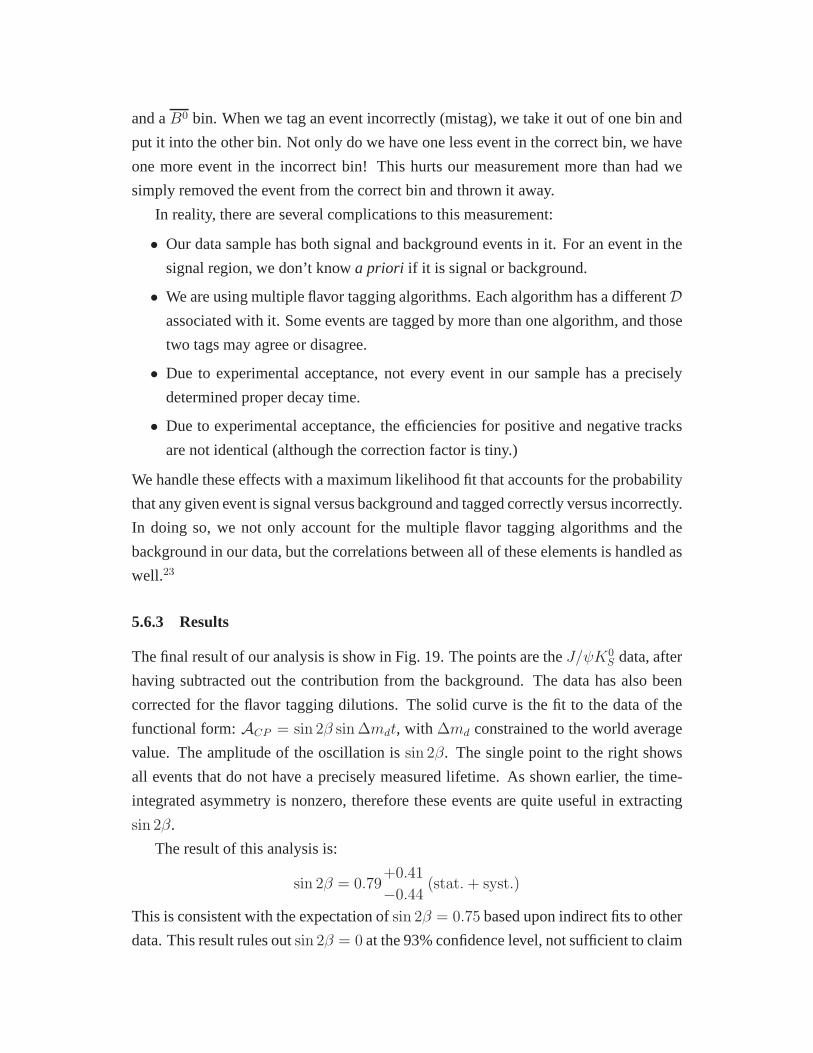
The final result of our analysis is show in Fig. 19. The points are theJ/ψK0S data, after

having subtracted out the contribution from the background. The data has also been

corrected for the flavor tagging dilutions. The solid curve is the fit to the data of the

functional form:ACP = sin 2β sin ∆mdt, with ∆md constrained to the world average

value. The amplitude of the oscillation issin 2β. The single point to the right shows

all events that do not have a precisely measured lifetime. Asshown earlier, the time-

integrated asymmetry is nonzero, therefore these events are quite useful in extracting

sin 2β.

The result of this analysis is:

sin 2β = 0.79+0.41

−0.44(stat.+ syst.)

This is consistent with the expectation ofsin 2β = 0.75 based upon indirect fits to other

data. This result rules outsin 2β = 0 at the 93% confidence level, not sufficient to claim

ct (cm)

true

asy

mm

etry

-1

0

1

2sin2β

-2

-1

0

1

2

3

4

0 0.05 0.1 0.15 0.2 0.25

Fig. 19. The true asymmetry (ACP (t) = sin 2β sin ∆mdt) as a function of lifetime for

B → J/ψK0S events. The data points are sideband-subtracted and have been combined

according to the effective dilution for single and double-tags. The events are shown in

the rightmost point are those that do not have precision lifetime information.

observation ofCP violation in theB system. On the other hand, this is the best direct

evidence to date forCP violation in theB system. When broken down into statistical

and systematic components, the uncertainty isδ(sin 2β) = ±0.39(stat.)± 0.16(syst.).

The total uncertainty is dominated by the statistics of the sample and efficacy of the

flavor tagging. The systematic uncertainty arises from the uncertainty in the dilution

measurements (δD.) However, the uncertainty on the dilution measurements are ac-

tually limited by the size of the data samples used to measurethe dilutions. In other

words, thesystematicuncertainty onsin 2β is really astatistical uncertainty on the

D’s. As more data is accumulated in the future, both the statistical and systematic

uncertainty insin 2β will decrease as1/√N .

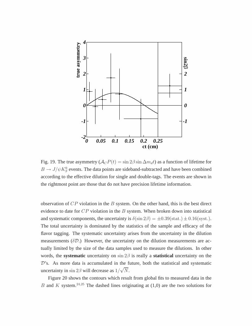
Figure 20 shows the contours which result from global fits to measured data in the

B andK system.24,25 The dashed lines originating at (1,0) are the two solutions for

sinCDF

ββ 2

S. Mele, hep-ph/9810333

ρ

η

68 % C.L.95 % C.L.

a)

∆ms

∆md

|εK||Vub|/|Vcb|

0

0.2

0.4

0.6

0.8

1

-1 -0.5 0 0.5 1

Fig. 20. The experimental determination ofρ andη. The curves are based upon experi-

mental measurements ofVub, ǫK , B0d andB0

s mixing. The contours are the result of the

global fit to the data.25 The dashed lines originating at (1,0) are the two solutions for β

corresponding tosin 2β = 0.79. The solid lines are the1σ contours for this result.

β corresponding tosin 2β = 0.79. The solid lines are the1σ contours for this result.

Clearly the result shown here is in good agreement with expectations.

The uncertainty on thesin 2β result presented here is comparable to the uncertain-

ties from recent measurements by the Belle and Babar collaborations.22,26 While none

of the measurements are yet to have the precision to stringently test the Standard Model,

the fact that this measurement can be made in two very different ways is interesting.

The hadron collider environment has an enormousbb cross section, but backgrounds

make flavor tagging difficult. In thee+e− environment, the production cross section is

much smaller, but the environment lends itself more favorably to flavor tagging. These

facts make the measurements performed in the different environments complementary

to one another.

5.7 The Future

The Fermilab Tevatron is scheduled to Run again in 2001. BothCDF14 and DØ13

detectors are undergoing massive upgrades in order to handle more than a factor of 20

increase in data. In addition,e+e− B-factories at Cornell (CLEO-III),27 KEK (Belle)28

and SLAC (BaBar)29 are all currently taking data. Finally, Hera-B,30 a dedicatedB

experiment at DESY, also will begin taking data in 2001.

On the timescale of 2003-2004, there could be as many as 5 different measurements

of sin 2β, all of them with an uncertainty ofδ(sin 2β) <∼ 0.1. Putting these together

would yield a world average measurement with an uncertaintyof δ(sin 2β) <∼ 0.05.

Although this alone will provide an impressive constraint upon the unitarity triangle, it

will not be sufficient to thoroughly test the Standard Model for self-consistency. On the

same timescale, improvements are required in the lengths ofthe sides of the triangle,

as well as other measurements of the angles. Finally, there are measurements of other

quantities that are not easily related to the unitarity triangle that are important tests of

the Standard Model.

The following is a list of some of the measurements that will be undertaken and/or

improved-upon in the coming years (this is an incomplete list):

• CP asymmetries in other modes:e.g.

– B0/B0 → π+π−;

– B0s/B

0s → J/ψφ;

– B0s/B

0s → K+K−;

– B0s/B

0s → D±

s K∓;

– B0/B0 → D+D−.

• B0s/B

0s mixing.

• rareB decays:e.g. B± → µ+µ−K±; B0 → µ+µ−.

• radiativeB decays:e.g. B0 → K∗γ; B0s → φγ.

• improved measurements ofVub: e.g. B → ππ; B → ρℓν.

• mass and lifetime of theBc meson.

• mass and lifetimes of theB baryons:e.g. Λb = |udb >.

It will take many years and a body of measurements to gain further insights into the

mechanisms behind the CKM matrix andCP violation.

Advances in kaon physics over the last 40 years and advances in B physics in the

last 25 years have put us on track to carry out these measurements in the very near fu-

ture. These measurements will hopefully bring us to a more fundamental understanding

to the mechanism behindCP violation.

Acknowledgments

I would like to thank David Burke, Lance Dixon, Charles Prescott and the organizers

of the 2000 SLAC Summer Institute. I would also like to thank and acknowledge the

collaborators of the CDF and DØ experiments, as well as the Fermilab accelerator

division. This work is supported by the U.S. Department of Energy Grant Number

DE-FG02-91ER40677.

References

[1] http://www-bd.fnal.gov/runII/index.html

[2] The CDF Collaboration (F. Abeet al.), Nucl. Instr. & MethA271, 387 (1988);

http://www-cdf.fnal.gov/.

[3] The DØ Collaboration (S. Abachiet al.), Nucl. Instr. & MethA338, 185 (1994);

http://www-d0.fnal.gov/.

[4] D. Cronin-Hennessy, A. Beretvas and P. Derwent, Nucl. Instr. & Meth A443, 37

(2000);

[5] The CDF Collaboration (T. Affolderet al.), Phys. Rev. Lett.84, 845 (2000); The

CDF Collaboration (F. Abeet al.), Phys. Rev.D59, 052002 (1999).

[6] The DØ Collaboration (B. Abbottet al.), Phys. Rev.D60, 052003, (1999).

[7] The DØ Collaboration (B. Abbottet al.), Phys. Rev.D61, 072001, (2000).

[8] The CDF Collaboration (F. Abeet al.), Phys. Rev.D52, 2624 (1995).

[9] E. Berger, F. Halzen, C.S. Kim and S. Willenbrock, Phys. Rev.D40, 83 (1989).

[10] The DØ Collaboration (B. Abbottet al.), Phys. Rev.D58, 092003, (1998); The

DØ Collaboration (B. Abbottet al.), Phys. Rev.D62, 092006, (2000).

[11] The CDF Collaboration (T. Affolderet al.), FERMILAB-PUB-00-158-E, (2000),

submitted to Phys.Rev.D.

[12] The LEP Electroweak Working Group, http://lepewwg.web.cern.ch/LEPEWWG/.

[13] The DØ Collaboration, FERMILAB-Pub-96/357-E (1996).

[14] The CDF-II Collaboration, FERMILAB-Pub-96/390-E (1996); The CDF-II Col-

laboration Fermilab-Proposal-909 (1998).

[15] J.H. Christensonet al., Phys. Rev. Lett.13, 138 (1964).

[16] N. Cabibbo, Phys. Rev. Lett.10, 531 (1963); M. Kobayashi and T. Maskawa,

Prog. Theor. Phys.49, 652 (1973).

[17] A.B. Carter and A.I. Sanda, Phys. Rev. Lett.45, 952 (1980); Phys. Rev. D23,

1567 (1981); I.I. Bigi and A.I. Sanda, Nucl. Phys.B193, 85 (1981); Nucl. Phys.

B281, 41 (1987).

[18] L. Wolfenstein, Phys. Rev. Lett.51, 1945 (1983).

[19] L.-L. Chau and W.-Y. Keung, Phys. Rev. Lett.53, 1802 (1984); C. Jarlskog and

R. Stora, Phys. Lett. B208, 268 (1988); J.D. Bjorken, Phys. Rev. D39, 1396

(1989).

[20] Y. Nir, IASSNS-HEP-99-96 (1999), hep-ph/9911321.

[21] Particle Data Group (C. Casoet al.), Eur. Phys. J. C3, 1 (1998); LEPB Oscilla-

tions Working Group, http://lepbosc.web.cern.ch/LEPBOSC/.

[22] C. Hearty, these proceedings.

[23] CDF Collaboration (T. Affolderet al.), Phys. Rev. D61:072005 (2000).

[24] S. Herrlich and U. Nierste, Phys. Rev. D52, 6505 (1995); A. Ali and D. London,

Nucl. Phys. B (Proc. Suppl.)54A, 297 (1997); P. Paganiniet al., Phys. Scr.58,

556 (1998).

[25] S. Mele, Phys. Rev. D59, 113011 (1999).

[26] N. Katayama, these proceedings.

[27] CLEO-III Collaboration, CLNS 94/1277 (1994).

[28] BELLE Collaboration, KEK Report 95-1 (1995).

[29] BaBar Collaboration, SLAC-Report-95-457 (1995).

[30] HERA-B Collaboration, DESY-PRC 95/01 (1995).