DYNAMICAL ELECTROWEAK SYMMETRY BREAKING AT TEVATRONRUN II AND LHC

By

Alexander Simon Blum

A THESIS

Submitted toMichigan State University

in partial fulfillment of the requirementsfor the degree of

MASTER OF SCIENCE

Department of Physics and Astronomy

2005

ABSTRACT

DYNAMICAL ELECTROWEAK SYMMETRY BREAKING AT TEVATRON

RUN II AND LHC

By

Alexander Simon Blum

The Standard Model (SM) of particle physics unifies the electromagnetic and the weak

force under an SU(2) x U(1) gauge group. The fact that these forces are observed

to be so different in strength and range is explained by spontaneous breaking of

this symmetry, induced by the nonzero vacuum expectation value of a scalar Higgs

field. There is however no experimental evidence for the Higgs field and there are also

theoretical difficulties. In one class of extensions of the SM designed to deal with these

problems, the electroweak symmetry is broken dynamically. This thesis provides a

framework in which SM Higgs searches at Tevatron Run II and at the Large Hadron

Collider (LHC) can be extended to new scalar or pseudoscalar states predicted in

dynamical models of electroweak symmetry breaking. These states can have enhanced

visibility in standard Higgs search channels, making them potentially discoverable at

Tevatron Run II and definitely visible at the LHC. I discuss the likely sizes of the

enhancements in the various search channels for each model and identify the model

features having the largest influence on the degree of enhancement. I suggest the mass

reaches of Higgs searches at Tevatron and LHC for these non-standard scalar states. I

compare signals for the non-standard scalars across models and also with expectations

in the SM and the Minimal Supersymmetric Model, another theory beyond the SM,

to show how one could start to identify which state has actually been found.

ACKNOWLEDGEMENTS

I would like to thank my advisor Professor Elizabeth Simmons, as well as Dr.

Alexander Belyaev and Professor Sekhar Chivukula for their constant input and sup-

port. I also would like to acknowledge a scholarship of the German National Academic

Foundation (Studienstiftung des deutschen Volkes).

iii

TABLE OF CONTENTS

LIST OF TABLES v

LIST OF FIGURES vi

1 Introduction 1

2 Higgs Searches and Enhancement Factors 3

3 Dynamical Electroweak Symmetry Breaking 53.1 General Remarks . . . . . . . . . . . . . . . . . . . . . . . . . . . . . 53.2 Technicolor . . . . . . . . . . . . . . . . . . . . . . . . . . . . . . . . 5

4 Results For Each Model 94.1 Technicolor . . . . . . . . . . . . . . . . . . . . . . . . . . . . . . . . 9

4.1.1 PNGB Production via Gluon Fusion . . . . . . . . . . . . . . 94.1.2 Production via Bottom Quark Annihilation . . . . . . . . . . 104.1.3 Decays . . . . . . . . . . . . . . . . . . . . . . . . . . . . . . . 13

4.2 Top-Pions . . . . . . . . . . . . . . . . . . . . . . . . . . . . . . . . . 14

5 Comparison and Interpretation 175.1 Technicolor vs SM . . . . . . . . . . . . . . . . . . . . . . . . . . . . 175.2 MSSM vs Technicolor . . . . . . . . . . . . . . . . . . . . . . . . . . . 195.3 Top-Pion vs Heavy SM Higgs . . . . . . . . . . . . . . . . . . . . . . 22

6 Conclusions 24

References 25

iv

LIST OF TABLES

1 Anomaly Factors for the models under study [23, 25, 30, 2, 3] . . . . 92 Calculated enhancement factors for production at the Tevatron and

LHC of a 130 GeV technipion via gg alone, via bb̄ alone, and combined.Note that the small enhancement in the bb̄ process slightly reduces thetotal enhancement relative to that of gg alone. . . . . . . . . . . . . . 10

3 Branching ratios of a technipion/Higgs of mass 130 GeV . . . . . . . 134 Branching ratio of top-pion/Higgs of mass 220 GeV . . . . . . . . . . 175 Enhancement Factors for 130 GeV technipions produced at the Teva-

tron, compared to production and decay of a SM Higgs Boson of thesame mass. The slight suppression of κP

prod due to the b-quark anni-hilation channel has been included.The rightmost column shows thecross-section (pb) for pp̄ → P → xx at Tevatron Run II. . . . . . . . 18

6 Enhancement Factors for 130 GeV technipions produced at the LHC,compared to production and decay of a SM Higgs Boson of the samemass. The slight suppression of κP

prod due to the b-quark annihila-tion channel has been included.The rightmost column shows the cross-section (pb) for pp̄ → P → xx at the LHC. . . . . . . . . . . . . . . . 19

7 Enhancement Factors for 220 GeV top-pions produced at the Teva-tron and the LHC, compared to production and decay of a SM HiggsBoson of the same mass. The slight suppression of κP

prod due to theb-quark annihilation channel is negligible.The rightmost column showsthe cross-section (pb) for pp̄ → P → xx at Tevatron Run II. . . . . . 23

v

LIST OF FIGURES

1 Total enhancement factor for each technicolor model plotted as a func-tion of technipion mass and assuming the final state is a tau (photon)pair. The lowest curve is the enhancement factor required to make aHiggs-like particle visible (5σ discovery) in tau(photon)-pairs at Teva-tron Run II with a total luminosity of 10 fb−1 [9], [38]. . . . . . . . . 20

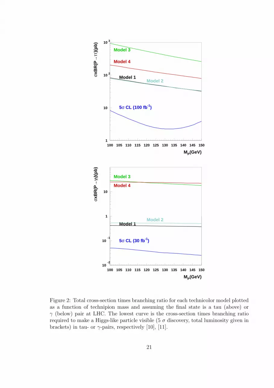
2 Total cross-section times branching ratio for each technicolor modelplotted as a function of technipion mass and assuming the final state isa tau (above) or γ (below) pair at LHC. The lowest curve is the cross-section times branching ratio required to make a Higgs-like particlevisible (5 σ discovery, total luminosity given in brackets) in tau- orγ-pairs, respectively [10], [11]. . . . . . . . . . . . . . . . . . . . . . . 21

vi

1 Introduction

Even though the electromagnetic and weak forces have been unified under a single

SU(2) x U(1) gauge group, the origin of the breaking of this electroweak symmetry

(manifest in the massless photon as gauge particle of the electromagnetic force com-

pared to the massive W and Z Bosons of the weak force) remains unknown. While the

Standard Model (SM) of particle physics, which accomplishes the symmetry breaking

by predicting a scalar Higgs field with nonzero vacuum expectation value, is consis-

tent with existing data, theoretical considerations show that this theory is only a

low-energy effective theory and must be supplanted by a more complete description

of the underlying physics at energies above those reached so far by experiment.

The CDF and D0 experiments at the Fermilab Tevatron are currently searching

for the Higgs boson of the Standard Model. The production cross-section and decay

branching fractions for this state have been predicted in great detail for the mass

range accessible to Tevatron Run II. Search strategies have been carefully planned

and optimized.

However, if the Tevatron does find evidence for a new scalar state, it may not

necessarily be the SM Higgs. Many alternative models of electroweak symmetry

breaking have spectra that include new scalar or pseudoscalar states whose masses

could easily lie in the range to which Run II is sensitive. The new scalars tend to

have cross-sections and branching fractions that differ from those of the SM Higgs.

The potential exists for one of these scalars to be more visible in a standard search

than the SM Higgs would be.

In this paper we provide a framework in which one can extract the maximum

possible information about the origin of electroweak symmetry breaking from SM

Higgs searches at Tevatron Run II and CERN LHC.

The idea of using standard Higgs searches to place limits on new scalar states

associated with electroweak symmetry breaking beyond the standard model has been

1

applied to LEP results (see e.g. Refs. [1, 2, 3, 4, 5, 6, 7, 8]). The Tevatron and

the LHC can potentially access significantly heavier scalars than those to which LEP

was sensitive, particularly in models of dynamical symmetry breaking. Reference [9]

has studied the potential of Tevatron Run II to search for the SM Higgs boson in

gg → hSM → ττ and determined what enhancement of the rate would be needed

to make a non-standard Higgs boson, e.g. from the Minimal Supersymmetric Model

(MSSM), a popular extension of the SM, visible in this channel. Similar studies

have been done for LHC for gg → hMSSM → ττ [10] and for gg → hSM → γγ [11]

processes.

My work builds on these results, considering an additional production mecha-

nism (b-quark annihilation), more decay channels (bb̄, WW , ZZ, and γγ), and, most

importantly, shifting the focus from theories of Supersymmetry to models of Dynam-

ical Electroweak Symmetry Breaking (DEWSB), an extension of the Standard Model

mentioned briefly in [9] and not at all in [10] and [11]. I discuss the likely sizes of

the enhancements in the various search channels for several different models and pin-

point the model features having the largest influence on the degree of enhancement. I

suggest the mass reach of the standard Higgs searches for each kind of non-standard

scalar state. I also compare the key signals for the non-standard scalars across models

and also with expectations in the SM and the MSSM, to show how one could start

to identify which state has actually been found.

In Section 2, I discuss Higgs searches and the enhancement factors needed to make

scalars of various masses visible. In Section 3, I talk about DEWSB in general and

show how to calculate elements of the enhancement factors in the various models. In

Section 4, I present my results for each model. In Section 5, I compare the different

models to one another and to the SM and MSSM. Section 6 holds my conclusions.

Part of this thesis will appear in a paper submitted for publication in June 2005

by Alexander Belyaev, R. Sekhar Chivukula, Elizabeth H. Simmons and me [12].

2

2 Higgs Searches and Enhancement Factors

As mentioned in the Introduction, [9] studied the potential of Tevatron Run II to

augment its search for the SM Higgs boson by considering the process gg → hSM →τ+τ−. While this channel would not suffice as a sole discovery mode,1 the authors

found that it could usefully be combined with other channels such as hSM → WW or

associated Higgs production to enhance the overall visibility of the Higgs. At the same

time, the authors determined what additional enhancement of scalar production and

branching rate, such as might be provided in a non-standard model like the MSSM,

would enable a scalar to become visible in the ττ channel alone at Tevatron Run II.

As these results are easily reinterpreted for DEWSB models, I take this as my

starting point, and examine how various Tevatron Run II searches for the SM Higgs

may provide information about the possible existence and properties of various Higgs-

like states that arise in DEWSB models. I look not only at the production and decay

channels which dominate in the SM, but also consider those which may be more

relevant in non-standard theories. I then go on (using [10] and [11]) to make some

predictions about visibility at the LHC.

Much of my discussion will focus on the degree to which certain standard Higgs

search channels are enhanced in non-standard models due to changes in the production

rate or branching fractions of the non-standard scalar (H) relative to the values for

the standard Higgs boson (hSM). I define the enhancement factor for the process

yy → H→ xx as the ratio of the products of the width of the (exclusive) production

mechanism and the branching ratio of the decay:

κHyy/xx =Γ(H → yy)×BR(H → xx)

Γ(hSM → yy)×BR(hSM → xx)= κHyy prod × κHxx dec (1)

1The authors established that discovery of hSM in this channel alone (assuming a mass in therange 120 - 140 GeV) would require an integrated luminosity of 14-32 fb−1, which is unlikely to beachieved.

3

I will consider both gluon fusion and bb̄ annihilation as possible production mecha-

nisms, and will study a variety of decay channels. Analytic formulas for the decay

widths of the SM Higgs boson are taken from [13], [14] and numerical values are

calculated using the HDECAY program [15] 2.

2With input parameters αs(M2Z) = 0.118, Mb = 4.60 GeV and Mt = 178 GeV.

4

3 Dynamical Electroweak Symmetry Breaking

3.1 General Remarks

The Standard Higgs Model of particle physics, based on the gauge group SU(3)c ×SU(2)W ×U(1)Y , accommodates electroweak symmetry breaking by including a fun-

damental weak doublet of scalar (“Higgs”) bosons φ =(

φ+φ0

)with potential function

V (φ) = λ(φ†φ− 1

2v2

)2. However the SM does not explain the dynamics responsible

for the generation of mass. Furthermore, the scalar sector suffers from two serious

problems. The scalar mass is unnaturally sensitive to the presence of physics at any

higher scale (e.g. the Planck scale), through contributions of loops of SM particles

to the Higgs self-energy. This is known as the gauge hierarchy problem [16]. In ad-

dition, if the scalar must provide a good description of physics up to arbitrarily high

scale (i.e., be fundamental), the scalar’s self-coupling (λ) is driven to zero at finite

energy scales. That is, the scalar field theory is free (or “trivial”) ( [17], [18]). Then

the scalar cannot fill its intended role: if λ = 0, the electroweak symmetry is not

spontaneously broken. The scalars involved in electroweak symmetry breaking must

therefore be a party to new physics at some finite energy scale – e.g., they may be

composite, as in the DEWSB models discussed here. The SM is merely a low-energy

effective field theory, and the dynamics responsible for generating mass must lie in

physics outside the SM.

In this section, I briefly introduce those aspects of dynamical electroweak symme-

try breaking which are most germane to my analysis. For a more complete introduc-

tion to dynamical electroweak symmetry breaking, see [19].

3.2 Technicolor

An intriguing class of models, generally referred to as dynamical electroweak symme-

try breaking models, supposes that the scalar states involved in electroweak symmetry

5

breaking could be manifestly composite at scales not much above the electroweak scale

v ∼ 250 GeV. In these theories, a new asymptotically free strong gauge interaction

(technicolor) breaks the chiral symmetries of approximately massless technifermions

f , which differ from the regular quarks and leptons of the SM in that they also carry a

technicolor charge, at a scale Λ ∼ 1 TeV ( [20], [21]). If the fermions carry appropriate

electroweak quantum numbers (e.g. left-handed weak doublets and right-handed weak

singlets), the resulting condensate 〈f̄LfR〉 6= 0 breaks the electroweak symmetry as

desired. Three of the Nambu-Goldstone Bosons (technipions) of the chiral symmetry

breaking become the longitudinal modes of the W and Z. The logarithmic running of

the strong gauge coupling renders the low value of the technicolor scale (and thereby

the electroweak scale) natural. The absence of fundamental scalars obviates concerns

about triviality.

Many models of DEWSB have additional light neutral pseudo Nambu-Goldstone

bosons (PNGBs) which could potentially be accessible to a standard Higgs search;

these are called “technipions” in technicolor models. There is not one particular

DEWSB model that has been singled out as a benchmark, in the manner of the

MSSM among supersymmetric theories. Rather, several different classes of models

have been proposed to address various challenges within the DEWSB paradigm of the

origins of mass. In this thesis, I look at several representative technicolor models. I

both evaluate the potential of standard Higgs searches to discover the lightest PNGBs

of each of these models, and also draw some inferences about the characteristics of

technicolor models that have the greatest impact on this search potential.

My analysis will assume, for simplicity, that the lightest PNGB state is signif-

icantly lighter than other neutral (pseudo)scalar technipions, so as to heighten the

comparison to the SM Higgs boson. The precise spectrum of any technicolor model

generally depends on a number of parameters, particularly those related to whatever

“extended technicolor” ([26, 31]) interaction transmits electroweak symmetry break-

6

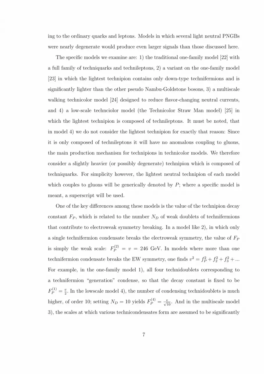
ing to the ordinary quarks and leptons. Models in which several light neutral PNGBs

were nearly degenerate would produce even larger signals than those discussed here.

The specific models we examine are: 1) the traditional one-family model [22] with

a full family of techniquarks and technileptons, 2) a variant on the one-family model

[23] in which the lightest technipion contains only down-type technifermions and is

significantly lighter than the other pseudo Nambu-Goldstone bosons, 3) a multiscale

walking technicolor model [24] designed to reduce flavor-changing neutral currents,

and 4) a low-scale technciolor model (the Technicolor Straw Man model) [25] in

which the lightest technipion is composed of technileptons. It must be noted, that

in model 4) we do not consider the lightest technipion for exactly that reason: Since

it is only composed of technileptons it will have no anomalous coupling to gluons,

the main production mechanism for technipions in technicolor models. We therefore

consider a slightly heavier (or possibly degenerate) technipion which is composed of

techniquarks. For simplicity however, the lightest neutral technipion of each model

which couples to gluons will be generically denoted by P ; where a specific model is

meant, a superscript will be used.

One of the key differences among these models is the value of the technipion decay

constant FP , which is related to the number ND of weak doublets of technifermions

that contribute to electroweak symmetry breaking. In a model like 2), in which only

a single technifermion condensate breaks the electroweak symmetry, the value of FP

is simply the weak scale: F(2)P = v = 246 GeV. In models where more than one

technifermion condensate breaks the EW symmetry, one finds v2 = f 2P + f 2

2 + f 23 + ...

For example, in the one-family model 1), all four technidoublets corresponding to

a technifermion “generation” condense, so that the decay constant is fixed to be

F(1)P = v

2. In the lowscale model 4), the number of condensing technidoublets is much

higher, of order 10; setting ND = 10 yields F(4)P = v√

10. And in the multiscale model

3), the scales at which various technicondensates form are assumed to be significantly

7

different, so that the lowest scale is simply bounded from above. In keeping with [24]

and to ensure that the technipion mass will be in the range to which the standard

Tevatron Higgs searches are sensitive, I set F(3)P = v

4.

In section 4, I study the enhancement factors for several production and decay

modes of the lightest eligible PNGBs of each technicolor model. Then in section 5, I

compare the signatures of these PNGBs to those of a SM Higgs and the Higgs bosons

of the MSSM in order to determine how the standard search modes (or additional

channels) can help tell these states apart.

In section 4.2, I briefly discuss topcolor models, in which new strong interactions

among top quarks form top-pion bound states with masses of order 2mt. The signa-

ture of this PNGB will then again be compared to the Higgs boson of the Standard

Model. I will always compare standard and non-standard scalars of the same mass,

so I will be comparing the top-pion with a rather heavy SM Higgs boson.

8

Table 1: Anomaly Factors for the models under study [23, 25, 30, 2, 3]

1) one-family 2) variant one-family 3) multiscale 4) low-scaleAgg

1√3

1√6

√2 1√

3

Aγγ − 43√

316

3√

64√

23

349

4 Results For Each Model

In this section, I examine the single production of technicolor PNGBs via the two

dominant methods at the Tevatron: gluon fusion and bb̄ annihilation. I determine

the degree to which these production channels are enhanced relative to production of

a SM Higgs, and find which channel dominates for each scalar state. I likewise study

the major decay modes: bb̄, ττ , γγ, and WW in order to determine the branching

fractions relative to those of an SM Higgs.

4.1 Technicolor

4.1.1 PNGB Production via Gluon Fusion

Single production of a technipion can occur through the axial-vector anomaly which

couples the technipion to pairs of gauge bosons. For an SU(NTC) technicolor group

with technipion decay constant FP , the anomalous coupling between the technipion

and a pair of gauge bosons is given, in direct analogy with the coupling of a QCD

pion to gluons, by [27, 28, 29]

NTCAV1V2g1g2

8π2FP

εµνλσkµ1 kν

2ελ1ε

σ2 (2)

where AV1V2 is the anomaly factor (determined by the symmetry structure of the

model), gi are the gauge boson couplings, and the ki and εi are the four-momenta

and polarizations of the gauge bosons. The values of the anomaly factors for the

lightest PNGB coupling to gluons is given in Table 1 for each model.

9

Table 2: Calculated enhancement factors for production at the Tevatron and LHC of a 130GeV technipion via gg alone, via bb̄ alone, and combined. Note that the small enhancementin the bb̄ process slightly reduces the total enhancement relative to that of gg alone.

1) one family 2) variant one-family 3) multiscale 4) low scaleκP

gg prod 48 6 1100 120κP

bb prod 4 0.67 16 10κP

total prod 47 5.9 1100 120

The rate of single technipion production in this channel is proportional to the

decay width to gluons. In the technicolor models, we have

Γ(P → gg) =1

2

8

32πm3

P

(αsNTCAgg

2πFP

)2

. (3)

while in the SM, the expression looks like [13]

Γ(h → gg) =1

2

8

32πm3

h

(αs3πv

)2

(4)

Comparing a PNGB to a SM Higgs boson of the same mass, we find the enhancement

in the gluon fusion production rate is

κgg prod =Γ(P → gg)

Γ(h → gg)=

9

4N2

TCA2gg

v2

F 2P

(5)

The main factors influencing κgg prod for a fixed value of NTC are the anomalous

coupling to gluons and the technipion decay constant. The value of κgg prod for each

model (taking NTC = 4) is given in Table 2.

4.1.2 Production via Bottom Quark Annihilation

The PNGBs couple to b-quarks courtesy of the extended technicolor interactions re-

sponsible for producing masses for the ordinary quarks and leptons. The extended

technicolor (ETC) group (of which SU(NTC) is an unbroken subgroup) includes gauge

10

bosons that couple to both ordinary and technicolored fermions so that the ordinary

fermions can interact with the technicondensates that break the electroweak symme-

try.

The rate of technipion production via bb̄ annihilation is proportional to Γ(P → bb̄).

In general, the expression for the decay of a technipion to fermions is

Γ(P → ff) =NC λ2

f m2f mP

8π F 2P

√√√√1− 4m2f

m2P

S

(6)

where NC is 3 for quarks and 1 for leptons. The phase space exponent S is 3 for

scalars and 1 for pseudoscalars; the lightest PNGB in models 1) and 4) is a scalar,

while in models 2) and 3) it is assumed to be a pseudoscalar. For the technipion

masses considered here, the value of the phase space factor in (6) is so close to one

that the value of s makes no practical difference. The factor λf is a non-standard

Yukawa coupling distinguishing leptons from quarks. Model 2) has λquark =√

23

and

λlepton =√

6; model 3) also includes a similar factor, but with average value 1. Finally,

it should be noted that Model 2) assumes that the lightest technipion is composed

only of down-type fermions and cannot decay to cc̄; since this decay would usually

have a small branching ratio and cc̄ is not a preferred final state for Higgs searches,

this has little impact.

For comparison, decay width of the SM higgs into b-quarks is:

Γ(h → bb) =3 m2

b mh

8π v2

√√√√1− 4m2b

m2h

3

(7)

The production enhancement for bb̄ annihilation is (again assuming Higgs and Tech-

nipion have the same mass):

κbb prod =Γ(P → bb)

Γ(h → bb)=

λ2b v2

F 2P

√√√√1− 4m2b

m2h

S−3

(8)

11

The value of κbb prod (shown in Table 4) is controlled by the size of the technipion

decay constant.

We see from Table 2 that κbb prod is at least one order of magnitude smaller than

κgg prod in each model. Taking the ratio of equations (5) and (8)

κgg prod

κbb prod

=9

4N2

TCA2ggλ

−2b (9)

we see that the larger size of κgg prod is due to the factor of N2TC coming from the

fact that gluons couple to a technipion via a techniquark loop. The ETC interactions

coupling b-quarks to a technipion have no such enhancement.

In addition, the production cross-section for a SM Higgs boson via bb̄ annihilation

is 2 to 3 orders of magnitude smaller than that for gluon fusion at the Tevatron [32]

and the LHC [33]. With a smaller SM cross-section and a smaller enhancement factor,

it is clear that technipion production via bb̄ annihilation is negligible at Tevatron and

LHC. However, since including the bb̄ production channel reduces the enhancement

in general, I will include it in my calculations to get a more conservative estimate. I

therefore define a combined total enhancement factor:

κHtotal/xx =σ(gg → H→ xx) + σ(bb → H→ xx)

σ(gg → hSM → xx) + σ(bb → hSM → xx)

=κHgg/xx + σ(bb → H→ xx)/σ(gg → hSM → xx)

1 + σ(bb → hSM → xx)/σ(gg → hSM → xx)

=κHgg/xx + κHbb/xxσ(bb → hSM → xx)/σ(gg → hSM → xx)

1 + σ(bb → hSM → xx)/σ(gg → hSM → xx)

≡ [κHgg/xx + κHbb/xxRbb:gg]/[1 + Rbb:gg]. (10)

Here Rbb:gg is the ratio of bb̄ and gg initiated Higgs boson production, at Tevatron

and LHC respectively, in the Standard Model. The total production enhancement is

also given in Table 2. Note that the small differences in Rbb:gg between Tevatron and

12

Table 3: Branching ratios of a technipion/Higgs of mass 130 GeV

Decay 1) one family 2) variant 3) multiscale 4) low scale SM HiggsChannel one family

bb 0.60 0.53 0.23 0.60 0.53cc 0.05 0 0.03 0.05 0.02

τ+τ− 0.03 0.25 0.01 0.03 0.05gg 0.32 0.21 0.73 0.32 0.07γγ 2.7× 10−4 2.9× 10−3 6.1× 10−4 6.4× 10−3 2.2× 10−3

W+W− 0 0 0 0 0.29

LHC are negligible, so we get the same total production enhancement for both.

4.1.3 Decays

The decay width of a light technipion into gluons or fermion/anti-fermion pairs has

been discussed above. Since, in the interesting mass range, the technipions do not

decay to W bosons and decays to Z Bosons (through the axial vector anomaly) are

negligible, the remaining possibility is a decay to photons. Again, this proceeds

through the axial vector anomaly (cf. Equation (2)) and the anomaly factors Aγγ are

shown in Table 3.

I now calculate the technipion branching ratios from the above information, taking

NTC = 4. The values are essentially independent of the size of mP within the range

120 GeV - 160 GeV; the branching fractions for mP = 130 GeV are shown in Table 5.

The branching ratios for the SM Higgs at NLO are given for comparison; they were

calculated using HDECAY [15]. Note that, in contrast to the technipions, a SM Higgs

in this mass range already has a noticeable decay rate to off-shell vector bosons.

Comparing the technicolor and SM branching ratios in Table 5, we see immediately

that decay enhancements will be generally of order one, and therefore much smaller

than the production enhancements. Decays to bb̄ are slightly enhanced, if at all.

Decays to cc̄ are enhanced in our tree-level calculations – but note that it is higher-

order corrections that suppress this mode for the SM higgs; in any case, this is

13

not a primary discovery channel. Decays to τ leptons have a small enhancement

in general; again, the comparison of tree-level technicolor and loop-level SM Higgs

calculations may be a factor here. Model 2) is an exception; its unusual Yukawa

couplings yield a decay enhancement in the ττ channel of order the technipion’s

(low) production enhancement. In the γγ channel, the decay enhancement strongly

depends on the group-theoretical structure of the model, through the anomaly factor.

Table 6 includes the decay enhancements κPdec for the most experimentally promising

search channels.

4.2 Top-Pions

For additional comparison, I discuss a different DEWSB model, a topcolor-assisted

Technicolor (TC2) model ([34], [35], [36]), which I will be referring to as model 5).

TC2 models address the difficulty of simultaneously generating the large mass of the

top quark (which places an upper bound on the symmetry breaking scale ΛETC of the

ETC gauge group) and suppressing the experimentally-not-observed flavor-changing

neutral currents (FCNC), which can show up as a relic of ETC symmetry breaking

at low energies (thereby placing a lower bound on ΛETC). In these models, the

top quark mass is partially generated by another new strong interaction (topcolor)

between top quarks. The Higgs-like scalar here is a heavy top-pion, which I will be

referring to as T, since it is very different from the PNGBs of the other examples. T

is a linear combination of technipions and the composite scalars created by top quark

condensation.

In the TC2 model 5), there are two scales, one for technifermion condensation and

the other for top condensation. FT , the scale of top-pion condensation, is thereby,

as in model 3), only bounded from above. As I am taking the phenomenological

expressions from [37], I will also adhere to their choice of parameters, setting FT =

70 GeV.

14

Model 5) requires a top-pion heavier than the top quark, so we can not calculate

the anomalous coupling to gauge bosons in the limit mH ¿ mt. Instead we must

insert the mass-dependent function ([37])

A(5)gg = 4

m2t

m2T

√1− F 2

T

v2(1− ε) arcsin2 (

mT

2mt

) (11)

Further parameters need explaining here: ε denotes the fraction of the top mass

generated by ETC-interactions (as opposed to being generated by topcolor interac-

tions). We will set it to be ε = 0.01 (It must be on the order of the ratio of bottom

to top quark mass). mt is the top quark mass. Note that there is no equivalent to

the NTC parameter of technicolor models. Also it is important to mention, that the

square-root is neither a real anomaly nor a phase-space factor: it reflects the mixing

of techni- and top-pions and will show up several times Using equation 5 we then find,

setting mP = 220GeV (a value at the lower end of, but well within, the theoretically

predicted top-pion mass range)

κTgg prod = 36

m4t

m4T

(v2

F 2T

− 1)(1− ε)2 arcsin4 (mT

2mt

) ≈ 34. (12)

The top-pion of 5) couples most strongly to the third generation of quarks. It is

expected to be heavier than the technipions of the other models, but since it is not

heavier than 2mt, its main fermionic decay mode is:

Γ(T → bb) =NC

8πmT (

1

F 2T

− 1

v2)(mb − ms

mcε mt)

2

√√√√1− 4m2b

m2T

(13)

where the slight correction to mb arises because there are two distinct sources of the

mass of the bottom quark(ETC and topcolor). The charm and strange masses are

denoted mc and ms respectively.

We then get for the production enhancement by bottom quark annihilation (again

setting mT = 220 GeV):

15

κTbb prod = (1− 4m2

b

m2P

)−1(v

FT mb

(mb − msmc

ε mt))2 ≈ 9.6 (14)

Comparing this with the production enhancement for gluon fusion (Equation 14),

we see that the production enhancements are of the same order of magnitude. Even

though we expect a somewhat larger impact of bottom quark annihilation as a pro-

duction mechansim (since the factor of N2TC does not appear in this model), it turns

out that it is in fact negligible at the Tevatron and at the LHC for model 5).

Model 5) has a second fermionic decay mode for the top-pion - T is heavier then

a top quark and due to flavor-non-universality has the following FCNC decay mode:

Γ(T → tc) = K2tcNC

1

8π(

1

F 2T

− 1

v2)(mt(1− ε))2mT

√√√√1− m2t

m2T

(15)

The factor Ktc is included in the coupling, and must be kept small due to exper-

imental constraints. Following [37], I set it to be Ktc = 0.05. Again, the PNGBs of

model 5) do not decay to W bosons and anomalous decay to Z bosons is negligible,

so we are left with decay to photons, where, for the same reasons as for gluons, we

have to insert the following mass-dependant function instead of the anomaly factor:

A(5)γγ =

16

3

4m2t

m2T

√1− F 2

T

v2(1− ε) arcsin2 (

mT

2mt

) (16)

The ”pure” anomaly factor, derived from the group theoretical structure of the

coupling is the 163

at the beginning of the equation (note that this was 1 in the case

of gluons). The branching ratios for the top-pion (Table 4) are again calculated using

a mass of 220 GeV.

16

Table 4: Branching ratio of top-pion/Higgs of mass 220 GeV

Decay 5) Topcolor-assisted TC Heavy SM Higgsbb 0.26 1.7× 10−3

tc 0.63 0gg 0.11 0.69× 10−3

γγ 1.4× 10−3 3.7× 10−5

W+W− 0 0.71ZZ 0 0.29

5 Comparison and Interpretation

5.1 Technicolor vs SM

My results for the Tevatron Run II (LHC) production enhancements (including both

gg fusion and bb̄ annihiliation), decay enhancements, and overall enhancements of each

technicolor model relative to the SM are shown in Table 5 (6) for a technipion or Higgs

mass of 130 GeV. Multiplying κPtot/xx by the cross-section for SM Higgs production

via gluon fusion [33] yields an approximate technipion production cross-section, as

shown in the right-most column of Table 5 (6).

In each technicolor model, the main enhancement of the possible technipion signal

relative to that of an SM Higgs arises at production, making the size of the technip-

ion decay constant the most critical factor in determing the degree of enhancement.

An equally important role is played by the number of technicolors, which is not as

apparent here, since I have assumed it to be the same for all the models I considered.

Still, along with the absence of decays to vector bosons for the technipions, the factor

of N2TC is responsible for the fact, that we actually observe a net enhancement for all

models and in all decay channels.

Each decay enhancement is in general of order 1, making it significantly smaller

than the typical production enhancement. In model 3) the decay “enhancement” is

actually a suppression, but a tiny one compared to the production enhancement. We

17

Table 5: Enhancement Factors for 130 GeV technipions produced at the Tevatron, comparedto production and decay of a SM Higgs Boson of the same mass. The slight suppressionof κP

prod due to the b-quark annihilation channel has been included.The rightmost columnshows the cross-section (pb) for pp̄ → P → xx at Tevatron Run II.

Model Decay mode κPprod κP

dec κPtot/xx Cross Section

bb 47 1.1 52 14 pb1) one family τ+τ− 47 0.6 28 0.77 pb

γγ 47 0.12 5.6 6.4× 10−3 pb

bb 5.9 1 5.9 1.8 pb2) variant τ+τ− 5.9 5 30 0.84 pbone family γγ 5.9 1.3 7.7 8.7× 10−3 pb

bb 1100 0.43 470 130 pb3) multiscale τ+τ− 1100 0.2 220 6.1 pb

γγ 1100 0.27 300 0.34 pb

bb 120 1.1 130 36 pb4) low scale τ+τ− 120 0.6 72 2 pb

γγ 120 2.9 350 0.4 pb

find that P → bb̄ is very similar to hSM → bb̄. In contrast, P → cc̄ generally has

significant decay enhancement. However, this may be an artifact of our comparing

a tree-level technicolor result to an NLO result for hSM ; radiative corrections to

hSM → cc̄ tend to suppress the branching fraction. The decay P → ττ generally has

a suppressed rate relative to SM expectations; again, this may relate to comparing

leading technicolor and NLO SM results. An exception is model 2), where the special

structure of the Yukawa coupling leads to a ττ decay enhancement of the same order

as the production enhancement. The P → γγ decay enhancement factor depends

strongly on the group-theoretic structure of the model through the anomaly factor,

ranging from a distinct enhancement in model 4) to a factor-of-10 suppression in

model 1).

The net result for the models considered is a distinct enhancement of the P signal

in each of the ττ , bb̄ and γγ search channels. Given the large QCD background for

the bb̄ final state, the ττ and γγ channels are likely to be the most promising ways

18

Table 6: Enhancement Factors for 130 GeV technipions produced at the LHC, comparedto production and decay of a SM Higgs Boson of the same mass. The slight suppressionof κP

prod due to the b-quark annihilation channel has been included.The rightmost columnshows the cross-section (pb) for pp̄ → P → xx at the LHC.

Model Decay mode κPprod κP

dec κPtot/xx Cross Section

bb 47 1.1 52 890 pb1) one family τ+τ− 47 0.6 28 48 pb

γγ 47 0.12 5.6 0.4 pb

bb 5.9 1 5.9 100 pb2) variant τ+τ− 5.9 5 30 52 pbone family γγ 5.9 1.3 7.7 0.55 pb

bb 1100 0.43 473 8000 pb3) multiscale τ+τ− 1100 0.2 220 380 pb

γγ 1100 0.27 300 21 pb

bb 120 1.1 130 2200 pb4) low scale τ+τ− 120 0.6 72 120 pb

γγ 120 2.9 350 25 pb

to discover a technipion. As illustrated in Figure 1, the available enhancement is

well above what is required to render the P of any of these models visible in the ττ

channel at the Tevatron. In models 3 and 4, the visibility in the γγ final state can be

even more striking, making this a possible discovery channel even at the Tevatron.

Of course since we have net enhancements in all cases, all these models should have

visible technipions at the LHC, where even an SM Higgs would be detectable in the

mass range I have considered (cf. Figure 2).

5.2 MSSM vs Technicolor

A brief comparison between the models I have been considering and the MSSM is in

order here. The MSSM is an alternate expansion of the Standard Model, addressing

similar problems as DEWSB models but taking a different approach, proposing a

symmetry of nature relating fermions and bosons. The MSSM introduces two Higgs

19

Model 1

5σ CL (10 fb-1)

Model 2

Model 3

Model 4

MP(GeV)

κ ττ

1

10

10 2

10 3

100 105 110 115 120 125 130 135 140 145 150

Model 1

5σ CL (10 fb-1)

Model 2

Model 3

Model 4

MP(GeV)

κ γγ

1

10

10 2

10 3

100 105 110 115 120 125 130 135 140 145 150

Figure 1: Total enhancement factor for each technicolor model plotted as a functionof technipion mass and assuming the final state is a tau (photon) pair. The lowestcurve is the enhancement factor required to make a Higgs-like particle visible (5σdiscovery) in tau(photon)-pairs at Tevatron Run II with a total luminosity of 10 fb−1

[9], [38].

20

Model 1

5σ CL (100 fb-1)

Model 2

Model 3

Model 4

MP(GeV)

σxB

R(P

→ττ

)(p

b)

1

10

10 2

10 3

100 105 110 115 120 125 130 135 140 145 150

Model 1

5σ CL (30 fb-1)

Model 2

Model 3

Model 4

MP(GeV)

σxB

R(P

→γγ

)(p

b)

10-2

10-1

1

10

100 105 110 115 120 125 130 135 140 145 150

Figure 2: Total cross-section times branching ratio for each technicolor model plottedas a function of technipion mass and assuming the final state is a tau (above) orγ (below) pair at LHC. The lowest curve is the cross-section times branching ratiorequired to make a Higgs-like particle visible (5 σ discovery, total luminosity given inbrackets) in tau- or γ-pairs, respectively [10], [11].

21

doublets which break the electroweak symmetry and give mass to the fermions of the

SM. Calculations similar to the ones I have done for DEWSB models in this thesis

are performed for supersymmetric models in the paper ”The Meaning of Higgs: τ+τ−

and γγ at the Tevatron and the LHC” [12] mentioned earlier. I describe some of the

major differences between DEWSB models and the MSSM here.

One notable difference concerns the production mechanism: While bottom quark

annihilation is, as we have seen, negligible for technipions, this channel can become

very important and even dominant in large sections of the MSSM parameter space.

The more important (since more observable) difference is however the difference

in branching rates for some important decay modes. While ττ decays are enhanced

in both models compared to the SM, decays to photons are heavily suppressed in

the MSSM as opposed to the moderate to large enhancements I have calculated for

technicolor models. While this will probably play no role in analyzing data from

Tevatron Run II, this significant difference could be the perfect way to distinguish

between these two non-standard models at the LHC.

5.3 Top-Pion vs Heavy SM Higgs

Model 5) has a special role for several reasons: Mainly of course, its main decay mode

is flavor changing and not even open to the SM higgs. But also, it necessitates a top-

pion with a mass beyond the WW-decay threshold, which can nonetheless not decay to

massive vector bosons. This absence of a signature is almost as striking as the FCNC,

since the SM Higgs boson has a branching ratio of almost 100 percent to massive vector

bosons at a mass of 220 GeV. So this model has very large decay enhancements (on the

order of the production enhancement) in it’s allowed decay channels, making it easily

detectable if the Higgs Search in this mass range is not limited to only vector-boson-

decays (whose mere absence would of course not necessarily indicate the existence of

the top-pion!). Note however the absence of leptonic decays, since leptons get their

22

Table 7: Enhancement Factors for 220 GeV top-pions produced at the Tevatron and theLHC, compared to production and decay of a SM Higgs Boson of the same mass. The slightsuppression of κP

prod due to the b-quark annihilation channel is negligible.The rightmostcolumn shows the cross-section (pb) for pp̄ → P → xx at Tevatron Run II.

Decay mode κPprod κP

dec κPtot/xx Cross Section (Tev) Cross Section (LHC)

bb 34 150 5100 0.77 pb 110 pbτ+τ− 34 0 0 0 pb 0 pbγγ 34 38 1290 4.2× 10−3 pb 0.6 pb

mass entirely from ETC.

The enhancement factors for 5) (Table 7) seem excessive at first glance, but that

is only because the branching ratios for non-vector-boson decays get extremely small

for the light SM higgs. The ratio of total width to mass for the top-pion is still of the

order of 0.1 percent, which is narrower than the SM Higgs of the same mass. Looking

at the estimated cross-sections brings things back into proportion. For example at

the Tevatron, the cross-section for pp̄ → P → bb̄ in model 5) is only about ten times

larger than that of pp̄ → h → W+W− in the SM, so we have a much less drastic effect

than just looking at the enhancement factors would indicate and it is unlikely that

top-pions could be detected at the Tevatron. Since the SM background for bb̄ decays

is probably still too large and the ττ mode is not allowed, the only feasible detection

channel at the LHC is the decay to photons. To my knowledge, no calculations have

been made for visibilty in the γγ channel at this mass range, since such a heavy

SM Higgs would be perfectly visible through its decays to vector bosons. It seems

probable however, that a top-pion would be detectable through decay to photons at

the LHC.

23

6 Conclusions

I have shown that searches for a Standard Model Higgs boson at Tevatron Run II and

LHC can provide significant results even if the electroweak symmetry is dynamically

broken. The new scalar and pseudoscalar states of DEWSB models can have en-

hanced visibility in standard τ+τ− and γγ search channels, making them potentially

discoverable at Tevatron Run II and CERN LHC. This enhancement mainly comes

from an increased production rate, rather than from differences in the branching frac-

tions. The model parameters exerting the largest influence on the enhancements are

NTC and the technipion decay constant.

I also considered a topcolor-assisted technicolor model and compared the top-pion

of this model with a heavy SM Higgs boson. I found that the experimental signatures

of top-pions are so different from the SM Higgs that it is less easy to simply transfer

predictions for the SM. The main conclusion to be drawn is that even for Higgs-like

particles with masses beyond the WW-threshold, the search should not be limited to

decays to vector bosons, which are so dominant in the SM.

For the technicolor models, where a direct comparison to the SM is easier, I

investigated the likely mass reach of the Higgs searches at Tevatron and LHC in

pp̄ → P → τ+τ− and pp̄ → P → γγ for each model and found that in all cases there

exist DEWSB models with visible scalar or pseudoscalar states, warranting a close

look even when predictions for the SM Higgs are far from promising, such as for decay

to photons at Tevatron Run II. The enhancement (or suppression) of pp̄ → P → γγ is

also the best way of distinguishing DEWSB models from supersymmetric extensions

of the standard model at the LHC.

24

References

[1] G. Rupak and E. H. Simmons, Phys. Lett. B 362, 155 (1995) [arXiv:hep-ph/9507438].

[2] V. Lubicz and P. Santorelli, Nucl. Phys. B 460, 3 (1996) [arXiv:hep-ph/9505336].

[3] K. R. Lynch and E. H. Simmons, Phys. Rev. D 64, 035008 (2001) [arXiv:hep-ph/0012256].

[4] R. Barate et al. [ALEPH Collaboration], Phys. Lett. B 565, 61 (2003)[arXiv:hep-ex/0306033].

[5] P. Bechtle [LEP Collaboration], Eur. Phys. J. C 33 (2004) S723 [arXiv:hep-ex/0401007].

[6] G. L. Kane, T. T. Wang, B. D. Nelson and L. T. Wang, Phys. Rev. D 71,035006 (2005) [arXiv:hep-ph/0407001].

[7] G. Abbiendi et al. [OPAL Collaboration], Eur. Phys. J. C 40, 317 (2005)[arXiv:hep-ex/0408097].

[8] G. Sguazzoni, Acta Phys. Slov. 55, 93 (2005) [arXiv:hep-ph/0411096].

[9] A. Belyaev, T. Han and R. Rosenfeld, JHEP 0307, 021 (2003) [arXiv:hep-ph/0204210].

[10] D. Cavalli et al., arXiv:hep-ph/0203056.

[11] R. Kinnunen, S. Lehti, A. Nikitenko and P. Salmi, J. Phys. G 31, 71 (2005)[arXiv:hep-ph/0503067].

[12] A. Belyaev, A. Blum, R. S. Chivukula and E. H. Simmons, arXiv:hep-ph/0506086.

[13] J. F. Gunion, H. E. Haber, G. L. Kane and S. Dawson, SCIPP-89/13

[14] J. F. Gunion, H. E. Haber, G. L. Kane and S. Dawson, arXiv:hep-ph/9302272.

[15] A. Djouadi, J. Kalinowski and M. Spira, Comput. Phys. Commun. 108, 56(1998) [arXiv:hep-ph/9704448].

[16] G. ’t Hooft, C. Itzykson, A. Jaffe, H. Lehmann, P. K. . Mitter, I. M. Singerand R. Stora, “Recent Developments In Gauge Theories. Proceedings, NatoAdvanced Study Institute, Cargese, France, August 26 - September 8, 1979”

[17] K. G. Wilson, Phys. Rev. B 4, 3184 (1971).

[18] K. G. Wilson and J. B. Kogut, Phys. Rept. 12, 75 (1974).

25

[19] C. T. Hill and E. H. Simmons, Phys. Rept. 381, 235 (2003) [Erratum-ibid. 390,553 (2004)] [arXiv:hep-ph/0203079].

[20] L. Susskind, Phys. Rev. D 20, 2619 (1979).

[21] S. Weinberg, Phys. Rev. D 13, 974 (1976).

[22] E. Farhi and L. Susskind, Phys. Rept. 74, 277 (1981).

[23] R. Casalbuoni, A. Deandrea, S. De Curtis, D. Dominici, R. Gatto and J. F. Gu-nion, Nucl. Phys. B 555, 3 (1999) [arXiv:hep-ph/9809523].

[24] K. D. Lane and M. V. Ramana, Phys. Rev. D 44, 2678 (1991).

[25] K. D. Lane, Phys. Rev. D 60, 075007 (1999) [arXiv:hep-ph/9903369].

[26] S. Dimopoulos and L. Susskind, Nucl. Phys. B 155, 237 (1979).

[27] S. Dimopoulos, S. Raby and G. L. Kane, Nucl. Phys. B 182, 77 (1981).

[28] J. R. Ellis, M. K. Gaillard, D. V. Nanopoulos and P. Sikivie, Nucl. Phys. B182, 529 (1981).

[29] B. Holdom, Phys. Rev. D 24, 157 (1981).

[30] R. S. Chivukula, R. Rosenfeld, E. H. Simmons and J. Terning, arXiv:hep-ph/9503202.

[31] E. Eichten and K. D. Lane, Phys. Lett. B 90, 125 (1980).

[32] M. Carena et al. [Higgs Working Group Collaboration], arXiv:hep-ph/0010338.

[33] M. Spira, Nucl. Instrum. Meth. A 389, 357 (1997) [arXiv:hep-ph/9610350].

[34] C. T. Hill, Phys. Lett. B 345, 483 (1995) [arXiv:hep-ph/9411426].

[35] K. D. Lane and E. Eichten, Phys. Lett. B 352, 382 (1995) [arXiv:hep-ph/9503433].

[36] K. D. Lane, Phys. Lett. B 433, 96 (1998) [arXiv:hep-ph/9805254].

[37] C. x. Yue, Q. j. Xu, G. l. Liu and J. t. Li, Phys. Rev. D 63, 115002 (2001)[arXiv:hep-ph/0012332].

[38] S. Mrenna and J. D. Wells, Phys. Rev. D 63, 015006 (2001) [arXiv:hep-ph/0001226].

26