arX

iv:h

ep-p

h/04

0819

8v4

9 A

ug 2

007

Probing Light Pseudoscalars with Light

Propagation, Resonance and Spontaneous

Polarization

Sudeep Dasa, Pankaj Jaina, John P. Ralstonb and Rajib Sahaa

aPhysics Department, IIT, Kanpur - 208016, IndiabDepartment of Physics & Astronomy,

University of KansasLawrence, KS-66045, USA

February 2, 2008

Abstract: Radiation propagating over cosmological distances can probelight weakly interacting pseudoscalar (or scalar) particles. The existence of aspin-0 field changes the dynamical symmetries of electrodynamics. It predictsspontaneous generation of polarization of electromagnetic waves due to modemixing in the presence of background magnetic field. We illustrate this by cal-culations of propagation in a uniform medium, as well as in a slowly varyingbackground medium, and finally with resonant mixing. Highly complicatedcorrelations between different Stokes parameters are predicted depending onthe parameter regimes. The polarization of propagating waves shows inter-esting and complex dependence on frequency, the distance of propagation,coupling constants, and parameters of the background medium such as theplasma density and the magnetic field strength. For the first time we studythe resonant mixing of electromagnetic waves with the scalar field, whichoccurs when the background plasma frequency becomes equal to the mass ofthe scalar field at some point along the path. Dynamical effects are foundto be considerably enhanced in this case. We also formulate the conditionunder which the adiabatic approximation can be used consistently, and findcaveats about comparing different frequency regimes.

1

1 Introduction

Light, weakly interacting spin-0 particles are predicted by many extensionsof the Standard Model of Particle Physics. Such field might arise as pseudo-Goldstone bosons of some spontaneously broken chiral symmetry (PQ) [1, 2,3], in supergravity theories [4, 5] and the low energy string action [6, 7, 8]as the Kalb-Ramond field. The mixing of light with pseudoscalar fields inpropagation has a long history. Karl and Clark [9] looked for “cosmologicalbirefringence” more than 20 years ago. Pseudoscalar-electromagnetic fieldmixing has long been explored by several authors [10, 11, 12, 13, 14, 15, 16].Our focus is to explore use of polarization observables that can separatemodels. Our calculations find that polarization evolution can sometimes behighly complicated and not easily estimated by simple dimensional argu-ments. Placing limits based on rough arguments and dimensional analysisis far from reliable. Recently Csaki et al [17] raised the possibility that su-pernova dimming might be caused by photon-pseudoscalar (γ − φ) mixing,re-igniting interest [18] in this problem. Whether or not supernovas dim, theoverall physics of propagation turns out to be quite interesting, and the sig-nals of polarization particularly sensitive to careful treatment. The varietyof effects is huge. As a result, one must question the validity of placing lim-its based simply on dimensional analysis or naive generalities. Instead, thelogic has to be reversed to seek particular effects contradicting conventionalphysics wherever they occur, and then investigate the causes.

There is another reason to consider polarization as a cosmological observ-able. Physical theories are not tested by fitting undetermined parameters:they are tested by testing their symmetries. The framework of general relativ-ity (GR) has certain symmetries by construction. Among these symmetriesis duality, which predicts that the polarization of light in free space does notchange. By the principle of Equivalence, GR then prescribes parallel trans-port of polarizations that are trivial in freely falling coordinates. It followsthat observations inconsistent with duality might rule out perturbations ofthe metric as a false signal. Another symmetry of unitarity prevents thespontaneous appearance of polarization in an unpolarized beam of light. Ifsuch features contradicting GR are observed, then it rules out GR as anexplanation of them, lifting a “degeneracy” of interpretation, and puttingresponsibility uniquely on something new.

There is one spectacular signal. A spin-0 field generically induces po-larization even in a completely unpolarized beam. Indeed such a field can

2

spontaneously polarize the CMB itself. The effect is simple and quite distinc-tive. We are emboldened to suggest that the absence of polarization effectsin propagation over cosmological distances, or in CMB derived quantities,would put stringent limits on the existence of a light spin-0 field. In thisregard we have eagerly awaited the release of WMAP data on CMB polar-ization while preparing this article. We feel that the time for discovery withpolarization observables may be ripe with this and other sources of datacoming in the future.

2 Symmetries of Light in the presence of spin-

0 field

The existence of a light scalar (or pseudoscalar) field changes the symmetriesof the propagation of light. We consider a spin-0 field φ coupled to theelectromagnetic field strength Fµν by the action

S =

∫

d4x√−g

[

− 1

4FµνF

µν + gφφ ǫµναβFµνF αβ

+g′φφFµνFµν + jµA

µ +1

2∂µφ∂µφ− 1

2m2

φφ2 + V (φ)

]

. (1)

We include a coupling to a current jµ for completeness, while in practice thisterm will lead to modified propagation such as plasma frequencies, etc. Forthe purposes to be developed the potential V (φ) can be ignored as a smallperturbation, and the metric g be replaced by a given background form. Notethat we have included coupling of φ to both ǫµναβF

µνF αβ and F µνFµν , sinceboth are allowed by the symmetries of the theory. If φ is a pseudoscalar,as we assume, then the coupling g′φ breaks parity symmetry. However thisapproximate feature of the low energy world is not a symmetry of Nature,being broken by the weak interactions physics. Even if the coupling g′φ istuned to zero at some scale, a coupling will be induced by radiative correc-tions. In the rest of the paper, however, we ignore g′φ since the limit on thiscoupling is much more stringent compared to the limit on gφ [19].

Free space electrodynamics has an interesting symmetry called duality. Inthe Hamiltonian density H in natural units, the electric and magnetic fields

3

~E and ~B can be rotated:(

~E ′

~B′

)

=

(

cos θ sin θ− sin θ cos θ

) (

~E~B

)

;

H =1

2~E2 +

1

2~B2 → H. (2)

Although a symmetry of the Hamiltonian density, duality is not a symmetryof the Lagrangian density, which changes by a pure divergence. Noether’stheorem represents this faithfully: the duality current Kµ is not conserved,but its divergence is an identity:

Kµ = ǫµναβAνF αβ;

∂µKµ = ǫµναβFµνF αβ. (3)

As a consequence of duality symmetry, ǫµναβFµνF αβ ∼ ~E · ~B, which is not

invariant, must be zero in a free-space plane wave. Otherwise symmetrywould permit rotating it into a different magnitude, which is a contradiction.The duality current is deeply related to the helicity density:

1

2K0 = i

~k

ω· ~A∗

k × ~Ek, (4)

where ~k is the wave number, ω the angular frequency and ~A× ~E is the canon-ical spin density.1 Thus duality symmetry implies separate conservation ofthe spin and orbital angular momentum of light in a ~k eigenstate. Now thecoupling of φ to ǫµναβF

µνF αβ breaks duality symmetry, allowing the helicityof photons to mix, and the plane of polarization of light to change in prop-agation – at least in the general case. Remarkably, the coupling of Eq. 1vanishes for a single plane wave: an isolated photon is “safe”. However lightcannot be protected under all possible conditions, and below we explore theeffects of a background magnetic field.

Let us contrast the φ-coupling with propagation in the usual cosmologicalmodel. In that event there is a coupling of light and gravity: the metric entersas an “optical medium” in the form of

S =

∫

d4x√−g

[

−1

4Fµνg

να(x)gµβ(x)Fαβ

]

. (5)

1Strictly speaking, photon spin depends on the gauge choice. The interpretation comes

from the gauge A0 = 0, which is nearly unique in having valid canonical spin and orbital

angular momenta.

4

The energy of this system can be written

H =1

2( ~D · ~E + ~B · ~H );

Dk = gν0(x)gµk(x)Fµν ;

Hk =1

2ǫijkg

νj(x)gµk(x)Fµν . (6)

This system has a new duality of rotating ~D and ~H into ~E and ~B. In acoordinate system where the metric is trivial, then ~D = ~E and ~H = ~B andthe state of polarization is preserved.

GR also maintains a symmetry under which the power transmitted scaleswith kinematic dependence on the scale factor, while the plane and magni-tudes of polarizations are preserved, in the sense of parallel transport alonggeodesics. The prediction of GR effects then consist of a coordinate trans-formation. In the isotropic, homogeneous metrics assumed in cosmology, theobservable result is a red-shift.

Free-space symmetries map into GR symmetries due to the principle ofequivalence. Thus conclusions about them do not hinge on particular solu-tions. With GR serving as a “null” theory, the effects of γ−φ mixing can beseparated and distinguished: simply observe the spontaneous polarization oflight during propagation, for instance.

2.1 Mixing Light with Pseudoscalars

Astrophysics constraints limit the coupling gφ to be very tiny, yet the enor-mous length scales of cosmology allows small cumulative effects to developinto large ones. Proceeding requires discussion of scales so that we can lin-earize Eq. 1 to discuss mixing of modes in propagation. There are twoimportant classes: background φ, where the electromagnetic field is solvedwith a fixed pseudoscalar field, and background ~B, where a combination ofthe electromagnetic field and φ are solved for a given magnetic field. Herewe set the background φ field to zero and put our effort on the second case.

We will use symbol ~B for the magnetic background, and ~B for the fieldin propagation: the total magnetic field is ~B + ~B. Although galactic andintergalactic ~B ∼ µG fields are small, their effects are likely to be largecompared to the effects of φ. A quick calculation shows that ~E/c and ~Bof a typically weak but observable signal, such as light from a QSO or the

5

CMB, are also small compared to µG. We seek to linearize consistently with~E/c << ~B, and ~B << ~B. There is a well-defined 3-state propagation problemof mixing 2 light polarizations with coupling to φ. We first obtain the non-covariant form of Maxwell equations, as follows, and with no approximations:

∇ · ~E = gφ∇φ · ( ~B + ~B) + ρ; (7)

∇× ~E +∂( ~B + ~B)

∂t= 0; (8)

∇× ~B − ∂ ~E

∂t= gφ

(

~E ×∇φ− ( ~B + ~B)∂φ

∂t

)

+~j; (9)

∇ · ( ~B + ~B) = 0. (10)

Here Bi + Bi = 12ǫijkF

jk and Ei = F 0i are the usual electric and magneticfields. Besides this we have the equation for the pseudoscalar field

∂2φ

∂t2−∇2φ+m2

φφ = −gφ~E · ( ~B + ~B) (11)

Gauge invariance is explicit and one can check current conservation directly,

~∇ ·~j +∂ρ

∂t= 0.

The dynamics of this coupled 3-field system are complicated and been visitedby various approximations in the literature.

We assume ~B solves the zeroeth order Maxwell equations with no φ back-ground. Our linearized equations for ~E/c << ~B, ~B << ~B are

∇ · ~E = gφ∇φ · ~B + ρ; (12)

∇× ~E +∂ ~B

∂t= 0; (13)

∇× ~B − ∂ ~E

∂t= −gφ

~B∂φ∂t

+~j; (14)

∇ · ~B = 0. (15)

These equations remain exactly consistent with current conservation, ~∇·~j+∂ρ/∂t = 0.

Proceed to get a wave equation for ~E by taking the curl of Faraday’s Law,and substituting into Eqs. 7, 9. Replacing ~B ∼ ~B gives

− ~∇2 ~E +∂2 ~E

∂t2= gφ

~B∂2φ

∂t2− gφ

~∇(~∇φ · ~B). (16)

6

In this equation the longitudinal part of ~E mixes with ~∇φ · ~B. That is, ~E isnot perfectly transverse in general when coupled to φ.

Continuing along these lines towards a general solution greatly increasesthe complexity of the equations. We will be content here to show illustrativecalculations restricted to the limit ~∇φ· ~B = 0. In this case ~E is transverse andthe system readily collapses to 2-state mixing. We have extensive calculationsfor the more general cases, but we feel this paper would not be improvedby introducing long and complex calculations. Our detailed calculationsshow that the numerical importance of BL 6= 0 effects for the parameterregions considered in this paper are negligible. The only exception to thismay possibly be in the case of resonance where the correction terms may belumped together with other parameters in any event. The virtue of ~∇φ· ~B = 0,even if it is not the most general case in practice, is that one can get a feelfor the rich interplay of several dimensionful scales including gφ, B, m2

φ, theplasma frequency ωp, and the propagation distance z. The amazing range ofphenomena one should seek observationally is well illustrated.

Requirement 0: Existing Physics Known physics of electromagneticpropagation in matter must be taken into account. It is well known that theplane of linearly polarized light rotates in a propagation through magnetizedplasma: the Faraday effect. Our symmetry arguments are consistent, becauseduality is broken by the coupling to electric (as opposed to magnetic) chargesand currents. Fortunately Faraday rotation is quite frequency dependent,and most important for low frequencies below the GHz regime.

We also take into account the practical “photon mass” in the form ofthe plasma frequency. It is not an effect that can be ignored, and we doincorporate it in the momentum-space propagation equations below.

Requirement 1: Phase Accuracy Observables depend on the wavenumber differences ∆k accumulating phase ∆θ by propagating over largedistances ∆z. An accurate approximation needs the absolute phase error

(symbol δ) to be small compared to π, namely δ( ∆k±∆z ) << 1. Thisrequirement becomes more and more demanding as ∆z → ∞. Everyonerecognizes this requirement, listed here for completeness. In the absence ofdegeneracies, the wave numbers of propagating waves can often be obtainedconsistently in powers of gφ, provided the corrections are controlled: seebelow.

7

Requirement 2: Gauge Invariance It is very important for all symme-tries to be respected, and in particular, any violation of gauge invariance isunacceptable. Fortunately our equations set up in a gauge invariant mannercoincide with the standard literature in the limit of ~B · ~B = 0.

Requirement 3: Respect for Limit Interchange Shortly we will solvethe propagation and present a common series expansion in g2

φ to simplifythe formulas. We will find that the series contains factors of the frequencyω. The limit of g2

φ fixed and small, and taking ω → ∞, does not commutewith ω fixed and g2

φ → 0. Since the frequency of a eV photon in units of thecosmological length scale is huge, while the coupling constants contemplatedfor φ is tiny, one needs to examine series expansions carefully to be sure theyapply to the problem being solved.

3 Pseudoscalar-Photon Mixing: Uniform Back-

ground

Choose the coordinate system with the z-axis along the direction of prop-agation of the wave and the x-axis parallel to the transverse componentof the background magnetic field ~BT . Seek solutions with harmonic timedependence e−iωt. Denote the component mixing by subscript ‖ and its per-

pendicular complement by subscript ⊥. Define symbol ~A = ~E/ω, whichsimplifies equations much like the vector potential, except there is no “i”and ~A is gauge invariant.

The perpendicular component A⊥ does not mix with φ. The wave equa-tion for the mixing of A|| and φ can be written as,

(ω2 + ∂2z )

(

A‖(z)φ(z)

)

−M

(

A‖(z)φ(z)

)

= 0 (17)

where the “mass matrix” or “mixing matrix” is

M =

(

ω2p −gφBT ω

−gφBT ω m2φ

)

, (18)

and BT is the magnitude of the vector ~BT . At this point we took into accountthe plasma frequency ω2

p, which is a (non-local) gauge invariant mass for ~E.

8

Transform to a new basis(

A‖(z)φ(z)

)

= O

(

A‖(z)

φ(z)

)

(19)

where O is the orthogonal matrix

O =

(

cos θ − sin θsin θ cos θ

)

(20)

which diagonalizes the mixing matrix in Eq. 17. Diagonalization gives

tan 2θ =2gφωBT

m2φ − ω2

p

(21)

with mass eigenvalues

µ2± =

ω2p +m2

φ

2± 1

2

√

(ω2p −m2

φ)2 + (2gφBT ω)2 . (22)

We list the leading order expansion in gφ, by which

µ2+ = ω2

p +g2BT

2ω2

ω2p −m2

φ

; (23)

µ2− = m2

φ − g2BT2ω2

ω2p −m2

φ

. (24)

We noted earlier that examination of scales is needed to justify this step.Consistency requires

g2BT2ω2

(ω2p −m2

φ)2<< 1. (25)

Continuing, the equations are written in the diagonal basis as

(ω2 + ∂2z )A‖ − µ2

+A‖ = 0

(ω2 + ∂2z )φ− µ2

−φ = 0 (26)

which can be easily solved to give

A‖(z) = A‖(0)ei(ω+∆A)z

φ(z) = φ(0)ei(ω+∆φ)z (27)

9

and

ω + ∆A =√

ω2 − µ2+ ≈ ω − µ2

+

2ω

ω + ∆φ =√

ω2 − µ2− ≈ ω − µ2

−

2ω(28)

We will always work in the limit ω2 >> µ2±, justifying retention of just the

leading terms. The phase difference ∆φ − ∆A in this limit is found to be

∆φ − ∆A ≈ 1

2ω

√

(ω2p −m2

φ)2 + (2gφBT ω)2 (29)

The perpendicular component A⊥ does not mix with φ and is given by

A⊥(z) = A⊥(0)eik0z (30)

where k0 =√

ω2 − ω2p ∼ ω − ω2

p/2ω.

3.0.1 Typical Scales and Units

We use parameters typical of the Virgo supercluster for illustration. Gener-ally the plasma frequency is given by

ω2p =

4παne

me=

ne

10−6cm−3

(

3.7 × 10−14eV)2

. (31)

For the supercluster, the plasma density ne ∼ 10−6 cm−3 and the magneticfield is of the order of 1 B ∼ 0.1µG coherent over a distance scale of order10 Mpc [20]. As mentioned earlier, use of typical B values in BT formulas isdone to take advantage of the transparent simplicity of that limit.

In the limit of mφ << ωp, there is a useful length scale l defined by

l =2ω

(ω2p −m2

φ)≈ ν

106 GHz0.04 Mpc (32)

where ν = ω2π

. We refer to this as the oscillation length in analogy with asimilar variable in neutrino physics [21]. The value 106 GHz ∼ 4 eV is ahandy upper order of magnitude for optical frequencies.

A typical upper limit [22, 23, 24, 25] on the coupling parameter gφ is6 × 10−11 GeV−1. In Fig. 1 below, we show results for gφ ∼ 10−12 GeV−1,more than one order of magnitude smaller than the limit. For a magneticfield of 0.1 µG we find that the product gφB can be expressed as gφB = 0.215Mpc−1. For convenience the scales are summarized in different units in Table1.

10

quantity typical value alternate unitsB 0.1 µ G 4.78 × 1049 Mpc−2

gφ 10−11GeV−1 6.4 × 10−50 Mpcωp 3.7 × 10−23GeV

√

ne

10−6cm−3 5.7 ×1015√

ne

10−6cm−3 Mpc −1

ω 10−5 - 1 eV 1.6 ×1024 - 1.6 × 1029 Mpc−1

Table 1: Typical values of dimensionful scales in different units. If not other-wise specified we use ~ = c = 1. The value of gφ listed is far below publishedlimits of gφ < 6 × 10−11 GeV−1 [22].

3.0.2 Small Mixing Limit: a Simple Example

For an example we examine the most innocuous case of mixing angle θ → 0.Specifically, this is the limit

gφωBT

|m2φ − ω2

p|<< 1.

By Eq. 25, the limit of small mixing is just the same limit in which the naiveTaylor expansion of Eq. 24 in small gφ ∼ 0 applies. In this limit E||, E⊥

and φ are the approximate propagation eigenstates. One might think thereare no observable effects, and in particular, there would be no substantial“dimming” of intensity.

However there is an important relative phase shift in propagation:

E||(z) = E||(0)ei(ω+∆A)z;

E⊥(z) = E⊥(0)eik0z.

The physically observable density matrix ρ is given by

ρ =

(

< E||E∗|| > < E||E

∗⊥ >

< E⊥E∗|| > < E⊥E

∗⊥ >

)

, (33)

where < > denotes the statistical averages occurring in propagation. Undercoherent conditions this result predicts a cumulative rotation of the plane ofa linear polarization due to the off-diagonal term:

E||E∗⊥(z) = E||E

∗⊥(0)ei(ω2

p/2ω−µ2+/2ω)z . (34)

So long as the mixing is small, we may insert the g2φ expansions of Eq. 24 and

predict the angle of rotation increases linearly with frequency. Yet there is

11

always a limit in which the frequency is large enough to cause strong mixing.We explore this for m2

φ << ω2p.

Let the magnitude of the phase angle between E|| and E⊥ be denoted χ.From Eq. 34 we have

χ = z(ω2

p

2ω− µ2

+

2ω) ∼ z

g2BT2ω

2ω2p

, ω <<ω2

p

gφBT;

χ < zgφBT . (35)

Using gφBT ∼ Mpc−1 as a typical value, the phenomenon of a rotating po-larization might be readily observed to be linear in ω at radio frequencies fordecades above the GHz regime.

Approaching the optical region, both the formula for small mixing andthe expansion of Eq. 24 break down, leading to very interesting possibilities.

3.0.3 Comments on Propagation

It is interesting to contrast the results above with propagation in a disper-sionless and non-dissipative medium, such as “free-space” with gravitationalfields. It is obvious that the intensity of a wave (Stokes I) is preserved upto the kinematic redshift of propagation 2. It is less obvious that the degree

of polarization (Stokes Q/I) cannot be changed by any 2-state purely elec-tromagnetic propagation in a dissipationless medium. The origin of this is“unitarity” of propagation which can be written as a unitary evolution oper-ator, just as in quantum mechanics [26]. As a consequence of 2-state electro-magnetic unitarity, a particular circular polarization (say) can be convertedinto a linear one, but a linear polarization cannot be made to come from anunpolarized ensemble. In the weak mixing region, an unpolarized densitymatrix (a multiple of the identity) evolves with no change whatsoever. Thismeans that basing observations or parameter limits on unpolarized quantitiescan easily miss effects that polarized observables would readily detect.

Spontaneous polarization is more than rare, and in pure electrodynamicsany form of polarization is usually associated with a corresponding extinc-tion. An ordinary polarizer plate is typical, with the degree of polarizationscaling directly with the degree of extinction. The same goes for commonsources of polarization such as Compton scattering invoked in astrophysics.

2Reflections, namely the generation of backwards moving waves, are always possible in

any varying medium. We work in the limit that they are negligible.

12

Momentarily we will discuss stronger mixing cases where mixing of light withpseudoscalars can lead to spontaneous polarization.

3.1 General Density Matrix

We can now determine the general density (coherency) matrix elements afterpropagation through distance z in terms of the matrix elements at the source.Inasmuch as we can interchange ~A with ~E/ω, it is convenient to report density

matrices of ~A. Then:

< A∗‖(z)A‖(z) > =

1

2< A∗

‖(0)A‖(0) >[

1 + cos2 2θ + sin2 2θ cos[z(∆φ − ∆A)]]

+< φ∗(0)φ(0) >

2

[

sin2 2θ − sin2 2θ cos[z(∆φ − ∆A)]]

+{< A∗

‖(0)φ(0) >

2

[

sin 2θ cos 2θ − sin 2θ cos 2θ cos[z(∆φ − ∆A)]

− i sin 2θ sin[z(∆φ − ∆A)]]

+ c.c.}

(36)

We gave the most general expression above keeping all the correlators atz = 0. One might think it reasonable to assume that < A∗

‖(0)φ(0) > is zero.However in considering propagation through an intergalactic medium oneexpects a large number of magnetic domains uncorrelated with one another.The general expression is needed to describe sequentially the propagationthrough different domains. Given the randomness of such processes, thegeneric situation is one where all the correlators on the right hand side willbe nonzero.

We also find,

< A∗‖(z)A⊥(z) > = (cos2 θeiF z + sin2 θeiGz) < A∗

‖(0)A⊥(0) >

+ cos θ sin θ(eiF z − eiGz) < φ∗(0)A⊥(0) > (37)

and < A∗⊥(z)A⊥(z) >=< A∗

⊥(0)A⊥(0) >. The phase factors F and G aregiven by

F = ω

√

1 −ω2

p

ω2− ω

√

1 − µ+

ω2≈ 1

2ω(µ+ − ω2

p)

G = ω

√

1 −ω2

p

ω2− ω

√

1 − µ−

ω2≈ 1

2ω(µ− − ω2

p)

13

Here again it is reasonable to expand F and G and keep only the leadingorder terms in ω2

p/ω2 and µ±/ω

2. Using these correlation functions we cancompute reduced Stokes parameters I, Q, U, V (or S0, S1, S2, S3)

I = < A∗‖(z)A‖(z) > + < A∗

⊥(z)A⊥(z) >

Q = < A∗‖(z)A‖(z) > − < A∗

⊥(z)A⊥(z) >

U = < A∗‖(z)A⊥(z) > + < A∗

⊥(z)A‖(z) >

V = i(− < A∗‖(z)A⊥(z) > + < A∗

⊥(z)A‖(z) > (38)

at any position z. The standard Stokes parameters of the same name aresimply ω2 times the above. We will often remove the scale of intensity,normalizing I = 2, as in an unpolarized wave |A|||2 = |A⊥|2 = 1.

3.1.1 Special Cases 1: Spontaneous Appearance of Polarization

Suppose the initial beam is unpolarized and the initial correlator< A∗‖(0)φ(0) >

is also zero. We scale out normalizations so that

< A∗‖(0)A‖(0) >=< A∗

⊥(0)A⊥(0) >= 1

and assume that all other correlators vanish at z = 0. The expressionssimplify to:

< A∗‖(z)A‖(z) > =

1

2

(

1 + cos2 2θ + cos[z(∆φ − ∆A)] sin2 2θ)

+1

2× < φ∗(0)φ(0) > (1 − cos[z(∆φ − ∆A)]) sin2 2θ (39)

< A∗‖(z)A⊥(z) > = 0 (40)

< A∗⊥(z)A⊥(z) > = 1 (41)

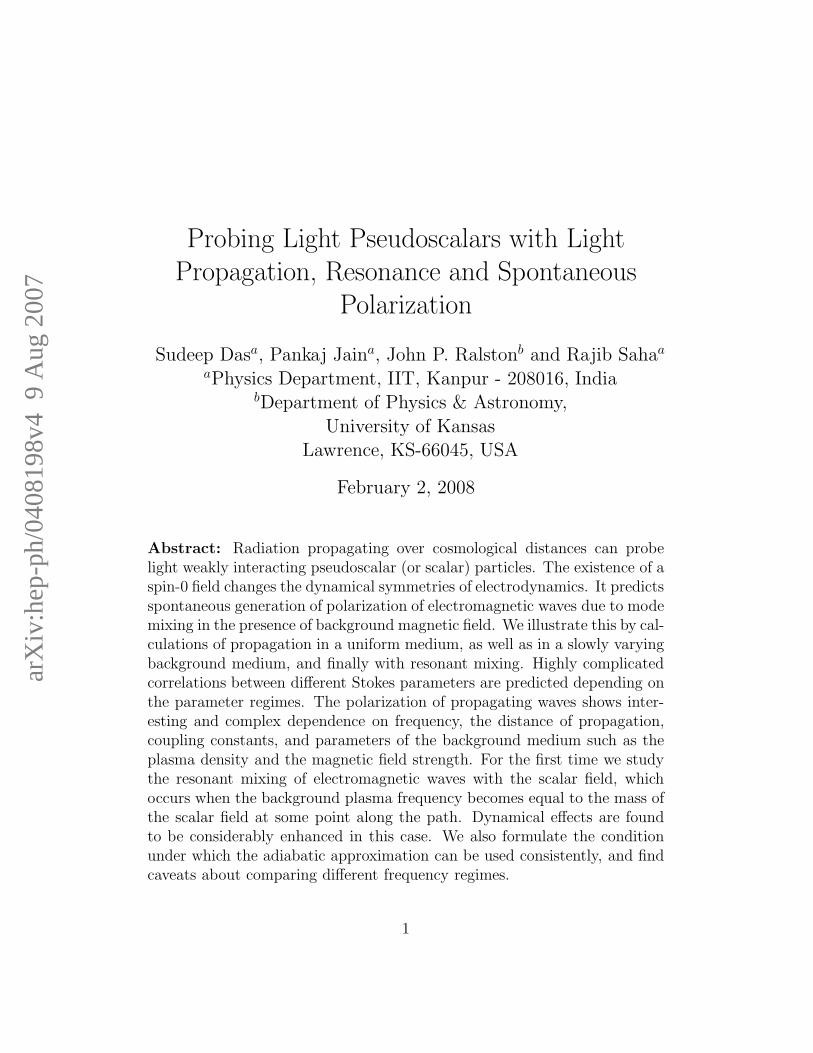
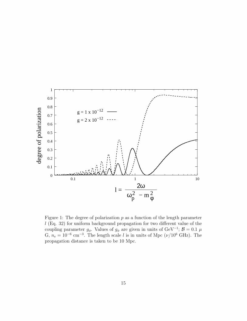
This wave spontaneously acquires a linear polarization oriented along ~Bduring propagation. No circular polarization is developed. We plot thedegree of polarization in Fig. 1 for initial conditions < φ∗(0)φ(0) >= 0. Thedegree of polarization p here is given by

p =|Q|I

=| < A∗

‖(z)A‖(z) > − < A∗⊥(z)A⊥(z) > |

< A∗‖(z)A‖(z) > + < A∗

⊥(z)A⊥(z) >, (42)

given Stokes U = V = 0. The degree of polarization accumulates to a sizeablemagnitude and could produce observable consequences even for exceedingly

14

2ωl =

ω2p − m2

φ

degr

ee o

f pol

ariz

atio

n

−12

−12

0

0.1

0.2

0.3

0.4

0.5

0.6

0.7

0.8

0.9

1

0.1 1 10

g = 1 x 10

g = 2 x 10

Figure 1: The degree of polarization p as a function of the length parameterl (Eq. 32) for uniform background propagation for two different value of thecoupling parameter gφ. Values of gφ are given in units of GeV−1; B = 0.1 µG, ne = 10−6 cm−3. The length scale l is in units of Mpc (ν/106 GHz). Thepropagation distance is taken to be 10 Mpc.

15

small couplings. In Fig. 1 the degree of polarization is shown for two differentvalues of the coupling parameter gφ = 1 × 10−12, 2 × 10−12 GeV−1. Thebackground medium parameters are chosen to be B = 0.1 µG and ne = 10−6

cm−3. The propagation distance is taken to be 10 Mpc. This is also thedistance over which the background magnetic field is assumed to be coherent.

The experimental signature of this mixing for a uniform backgroundwould require fitting the observed degree of polarization to a number ofparameters. As shown by the previous examples, the extrapolation betweenradio frequency and optical frequency observations needs care and attentionto series expansions. Nevertheless the spontaneous polarization due to mix-ing is clearly distinguishable from extinction, which is expected to show asimple monotonic increase in the degree of polarization with frequency.

3.1.2 Special Cases 2: Initial Polarization

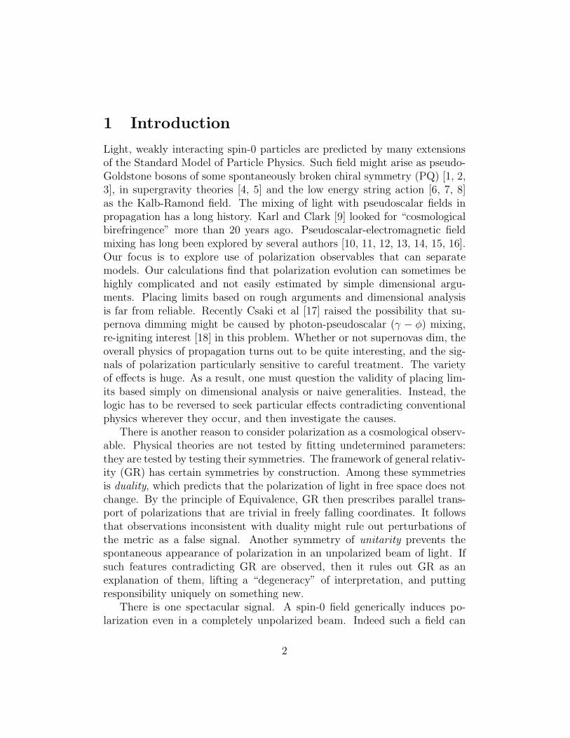
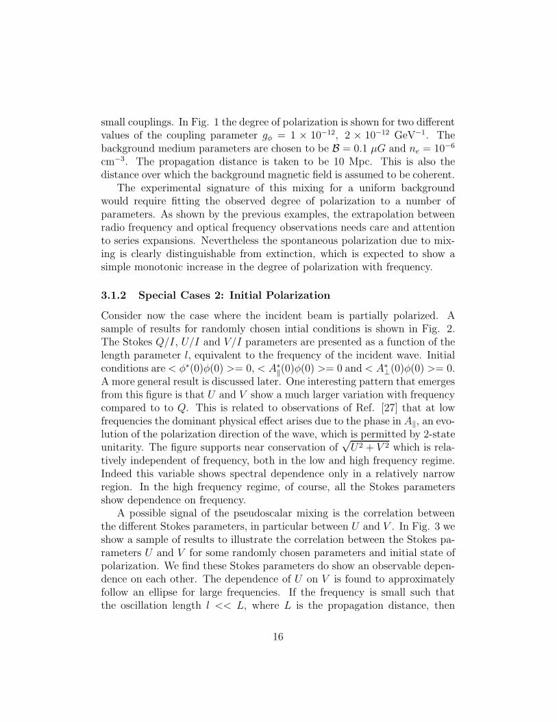
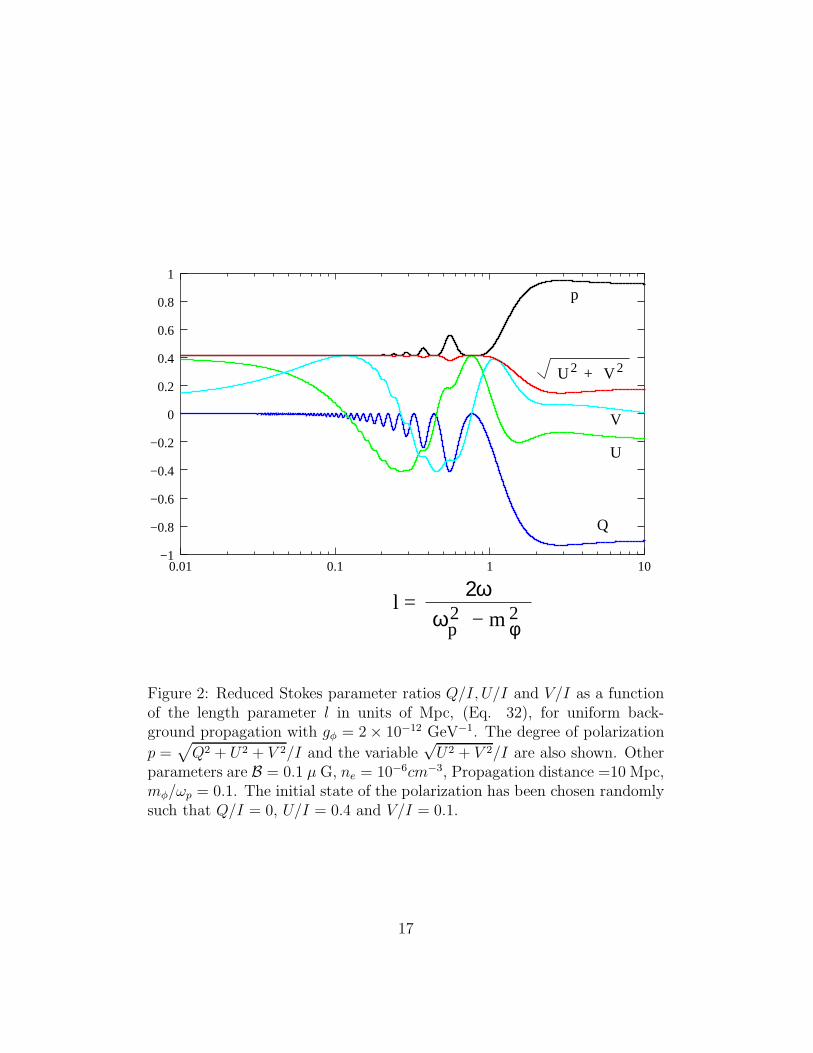
Consider now the case where the incident beam is partially polarized. Asample of results for randomly chosen intial conditions is shown in Fig. 2.The Stokes Q/I, U/I and V/I parameters are presented as a function of thelength parameter l, equivalent to the frequency of the incident wave. Initialconditions are < φ∗(0)φ(0) >= 0, < A∗

‖(0)φ(0) >= 0 and < A∗⊥(0)φ(0) >= 0.

A more general result is discussed later. One interesting pattern that emergesfrom this figure is that U and V show a much larger variation with frequencycompared to to Q. This is related to observations of Ref. [27] that at lowfrequencies the dominant physical effect arises due to the phase in A‖, an evo-lution of the polarization direction of the wave, which is permitted by 2-stateunitarity. The figure supports near conservation of

√U2 + V 2 which is rela-

tively independent of frequency, both in the low and high frequency regime.Indeed this variable shows spectral dependence only in a relatively narrowregion. In the high frequency regime, of course, all the Stokes parametersshow dependence on frequency.

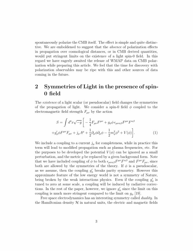
A possible signal of the pseudoscalar mixing is the correlation betweenthe different Stokes parameters, in particular between U and V . In Fig. 3 weshow a sample of results to illustrate the correlation between the Stokes pa-rameters U and V for some randomly chosen parameters and initial state ofpolarization. We find these Stokes parameters do show an observable depen-dence on each other. The dependence of U on V is found to approximatelyfollow an ellipse for large frequencies. If the frequency is small such thatthe oscillation length l << L, where L is the propagation distance, then

16

l = ω2

p − m2φ

2ω

2 2U V+

Q

V

U

p

−1

−0.8

−0.6

−0.4

−0.2

0

0.2

0.4

0.6

0.8

1

0.01 0.1 1 10

Figure 2: Reduced Stokes parameter ratios Q/I, U/I and V/I as a functionof the length parameter l in units of Mpc, (Eq. 32), for uniform back-ground propagation with gφ = 2 × 10−12 GeV−1. The degree of polarization

p =√

Q2 + U2 + V 2/I and the variable√U2 + V 2/I are also shown. Other

parameters are B = 0.1 µ G, ne = 10−6cm−3, Propagation distance =10 Mpc,mφ/ωp = 0.1. The initial state of the polarization has been chosen randomlysuch that Q/I = 0, U/I = 0.4 and V/I = 0.1.

17

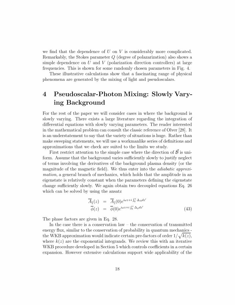
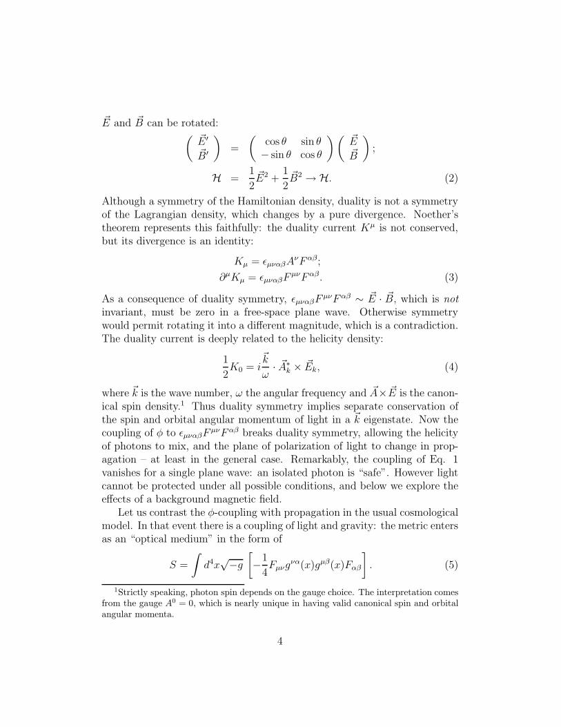
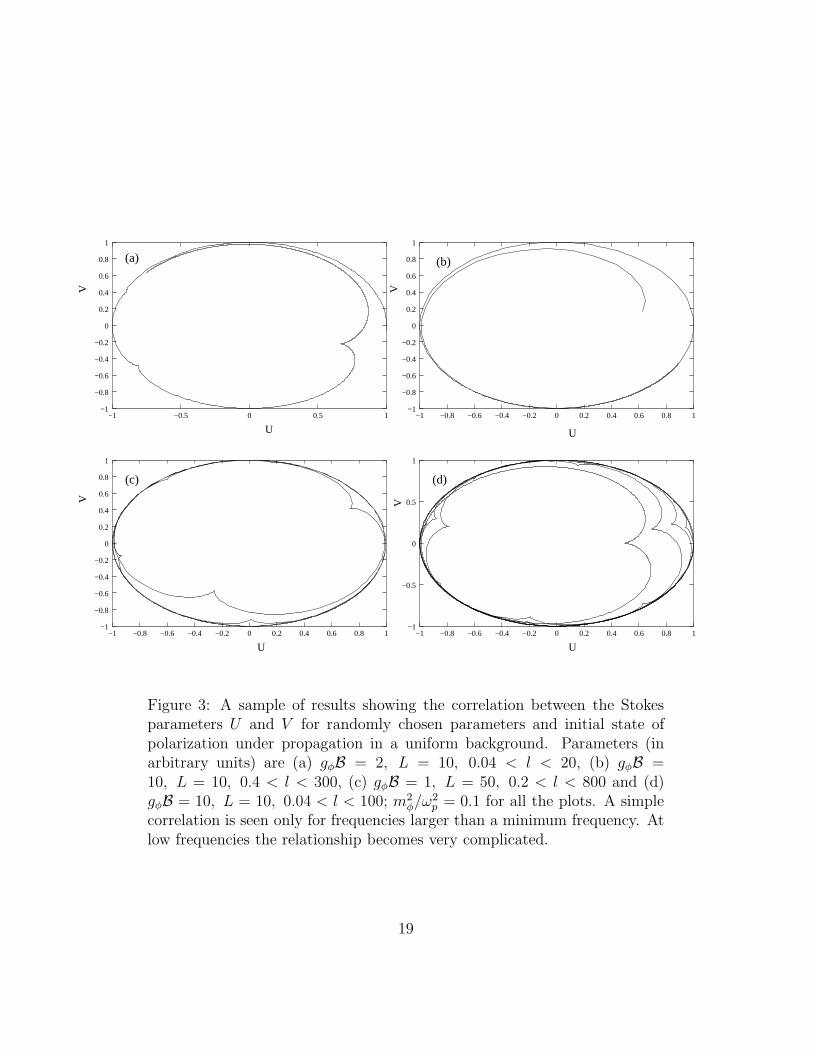
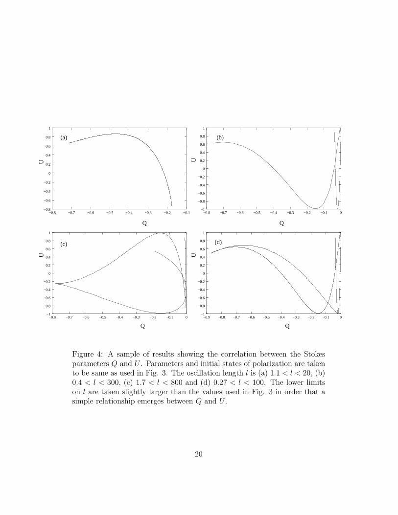
we find that the dependence of U on V is considerably more complicated.Remarkably, the Stokes parameter Q (degree of polazarization) also shows asimple dependence on U and V (polarization direction controllers) at largefrequencies. This is shown for some randomly chosen parameters in Fig. 4.

These illustrative calculations show that a fascinating range of physicalphenomena are generated by the mixing of light and pseudoscalars.

4 Pseudoscalar-Photon Mixing: Slowly Vary-

ing Background

For the rest of the paper we will consider cases in where the background isslowly varying. There exists a large literature regarding the integration ofdifferential equations with slowly varying parameters. The reader interestedin the mathematical problem can consult the classic reference of Olver [28]. Itis an understatement to say that the variety of situations is huge. Rather thanmake sweeping statements, we will use a workmanlike series of definitions andapproximations that we check are suited to the limits we study.

First restrict attention to the simple case where the direction of ~B is uni-form. Assume that the background varies sufficiently slowly to justify neglectof terms involving the derivatives of the background plasma density (or themagnitude of the magnetic field). We thus enter into the adiabatic approxi-

mation, a general branch of mechanics, which holds that the amplitude in aneigenstate is relatively constant when the parameters defining the eigenstatechange sufficiently slowly. We again obtain two decoupled equations Eq. 26which can be solved by using the ansatz

A‖(z) = A‖(0)eiωz+iR z0

∆Adz′

φ(z) = φ(0)eiωz+iR z

0∆φdz′ (43)

The phase factors are given in Eq. 28.In the case there is a conservation law – the conservation of transmitted

energy flux, similar to the conservation of probability in quantum mechanics -the WKB approximation would indicate certain pre-factors of order 1/

√

k(z),where k(z) are the exponential integrands. We review this with an iterativeWKB procedure developed in Section 5 which controls coefficients in a certainexpansion. However extensive calculations support wide applicability of the

18

V

U

V

U

V

U

V

(a) (b)

(c) (d)

U

−1

−0.8

−0.6

−0.4

−0.2

0

0.2

0.4

0.6

0.8

1

−1 −0.8 −0.6 −0.4 −0.2 0 0.2 0.4 0.6 0.8 1

−1

−0.8

−0.6

−0.4

−0.2

0

0.2

0.4

0.6

0.8

1

−1 −0.8 −0.6 −0.4 −0.2 0 0.2 0.4 0.6 0.8 1−1

−0.5

0

0.5

1

−1 −0.8 −0.6 −0.4 −0.2 0 0.2 0.4 0.6 0.8 1

−1

−0.8

−0.6

−0.4

−0.2

0

0.2

0.4

0.6

0.8

1

−1 −0.5 0 0.5 1

Figure 3: A sample of results showing the correlation between the Stokesparameters U and V for randomly chosen parameters and initial state ofpolarization under propagation in a uniform background. Parameters (inarbitrary units) are (a) gφB = 2, L = 10, 0.04 < l < 20, (b) gφB =10, L = 10, 0.4 < l < 300, (c) gφB = 1, L = 50, 0.2 < l < 800 and (d)gφB = 10, L = 10, 0.04 < l < 100; m2

φ/ω2p = 0.1 for all the plots. A simple

correlation is seen only for frequencies larger than a minimum frequency. Atlow frequencies the relationship becomes very complicated.

19

Q

U U

U U

Q

QQ

(a) (b)

(c) (d)

−1

−0.8

−0.6

−0.4

−0.2

0

0.2

0.4

0.6

0.8

1

−0.9 −0.8 −0.7 −0.6 −0.5 −0.4 −0.3 −0.2 −0.1 0

−0.8

−0.6

−0.4

−0.2

0

0.2

0.4

0.6

0.8

1

−0.8 −0.7 −0.6 −0.5 −0.4 −0.3 −0.2 −0.1−1

−0.8

−0.6

−0.4

−0.2

0

0.2

0.4

0.6

0.8

1

−0.8 −0.7 −0.6 −0.5 −0.4 −0.3 −0.2 −0.1 0

−1

−0.8

−0.6

−0.4

−0.2

0

0.2

0.4

0.6

0.8

1

−0.8 −0.7 −0.6 −0.5 −0.4 −0.3 −0.2 −0.1 0

Figure 4: A sample of results showing the correlation between the Stokesparameters Q and U . Parameters and initial states of polarization are takento be same as used in Fig. 3. The oscillation length l is (a) 1.1 < l < 20, (b)0.4 < l < 300, (c) 1.7 < l < 800 and (d) 0.27 < l < 100. The lower limitson l are taken slightly larger than the values used in Fig. 3 in order that asimple relationship emerges between Q and U .

20

simpler formulas, inasmuch as k(z) tends to cancel out of polarization ratiosand not to develop cumulative run-outs in many circumstances.

Using these results we can now evaluate the electromagnetic field at anyposition. For this purpose we express the fields A(0) and φ(0) in terms ofA‖(0) and φ(0) and the mixing angle θ(0). The final expressions for the fieldsA‖(z) and φ(z) are given by

A‖(z) = eiωzA‖(0)

[

cos θ cos θ0 exp

(

i

∫ z

0

∆Adz′

)

+ sin θ sin θ0 exp

(

i

∫ z

0

∆φdz′

)]

+ eiωzφ(0)

[

cos θ sin θ0 exp

(

i

∫ z

0

∆Adz′

)

− sin θ cos θ0 exp

(

i

∫ z

0

∆φdz′

)]

φ(z) = eiωzA‖(0)

[

sin θ cos θ0 exp

(

i

∫ z

0

∆Adz′

)

− cos θ sin θ0 exp

(

i

∫ z

0

∆φdz′

)]

+ eiωzφ(0)

[

sin θ sin θ0 exp

(

i

∫ z

0

∆Adz′

)

+ cos θ cos θ0 exp

(

i

∫ z

0

∆φdz′

)]

(44)

where on the right hand side θ = θ(z) and θ0 = θ(0). The resulting expres-sions for the coherency matrix elements is given by

< A∗‖(z)A‖(z) > =

< A∗‖(0)A‖(0) >

2[1 + cos 2θ cos 2θ0 + sin 2θ sin 2θ0 cos Φ]

+< φ∗(0)φ(0) >

2[1 − cos 2θ cos 2θ0 − sin 2θ sin 2θ0 cos Φ]

+(< A∗

‖(0)φ(0) >

2

[

cos 2θ sin 2θ0 − sin 2θ cos 2θ0 cos Φ

+ i sin 2θ sin Φ]

+ c.c.)

(45)

where

Φ =

∫ z

0

(∆A − ∆φ)dz′ (46)

< A∗‖(z)A⊥(z) > = < A∗

‖(0)A⊥(0) >[

cos θ cos θ0 exp

(

i

2ω

∫ z

0

dz′[µ2+ − ω2

p]

)

+ sin θ sin θ0 exp

(

i

2ω

∫ z

0

dz′[µ2− − ω2

p]

)

]

21

+ < φ∗(0)A⊥(0) >[

cos θ sin θ0 exp

(

i

2ω

∫ z

0

dz′[µ2+ − ω2

p]

)

− sin θ cos θ0 exp

(

i

2ω

∫ z

0

dz′[µ2− − ω2

p]

)

]

. (47)

The above result is valid as long as the medium changes slowly so that theterm

2OT (∂zO)∂z

(

Aφ

)

= 2iωθ′(

0 −11 0

)(

Aφ

)

(48)

is negligible compared to mass term(

µ2+ 00 µ2

−

) (

Aφ

)

.

We are justified in ignoring the derivative of the mixing angle θ if

|θ′| << µ2±

2ω(49)

The condition for adiabaticity will be formulated in greater detail in section5. There we estimate the transition probability from one local eigenstateto another. As we shall see, the condition given above, Eq. 49, is sufficientprovided the difference between µ+ and µ− is of the order of these eigenvalues.If there is a delicate cancellation between these two eigenvalues then on theright hand side in Eq. 49 more care and specialized techniques may beneeded.

4.1 Resonance

We next discuss the interesting case where the plasma frequency ωp becomesequal to the pseudoscalar massmφ somewhere along the path. Given the widerange of plasma frequencies observed in the astrophysics there may be manysituations where such resonance might occur. Examples include propagationof light or pseudoscalars from a dense medium, such as an AGN, GRB orcluster of galaxies into the intergalactic medium. Another example includespropagation of light from pulsar magnetosphere into the interstellar medium.Let the radiation initially propagate from the region z = 0 containing highplasma density ωp > mφ towards increasing z where a resonance occurs.Assume that initially the mixing angle θ << 1, and recall

tan 2θ =2gφωBT

m2φ − ω2

p

<< 1. (50)

22

Let the plasma density decrease slowly along the path such that at the ob-servation point mφ > ωp. Somewhere along the path at z = z∗ the righthand side of Eq. 50 becomes infinite, which we will implement with angle2θ(z∗) → π/2 . To finally fix the initial conditions, let < A∗

‖(0)A‖(0) > 6= 0,

< A∗‖(0)A⊥(0) > 6= 0 and < A∗

⊥(0)A⊥(0) > 6= 0 , that is, a generically mixedwave. The remaining correlators, which involve φ, are taken to be zero atz = 0. We compare the conditions after traveling a distance ∆z = L to theobservation point. From Eq. 45, 47 we find:

< A∗‖(L)A‖(L) > ≈ 0 ,

< A∗‖(L)A⊥(L) > ≈ 0 ,

< A∗⊥(L)A⊥(L) > = < A∗

⊥(0)A⊥(0) > (51)

if | tan 2θ| << 1 at z = L. These are predicted independent of frequency andthe distance travelled, provided the wave crosses the region where mφ = ωp.Almost independent of the state of polarization at the origin, the wave be-comes completely linearly polarized at the observation point. The orientationof the electric field vector is perpendicular to the background magnetic field.3

Studying resonance using a slowly varying approximation requires somecare. The consistent requirement is that the assumption of slowly varyingbackground be satisfied. We now make this assumption more precise inorder to obtain a constraint on the derivative of the background plasmafrequency. For this purpose we assume that the background plasma densityvaries linearly with position such that

m2φ

ω0

−ω2

p

ω0

= C − αz (52)

where C and α are constants, z is the distance of propagation and ω0 is somechosen value of the frequency of the wave. It is convenient to work with therescaled variables,

ω2p =

ω2p

ω0

, m2φ =

m2φ

ω0

, ω =ω

ω0

, (53)

3Generally all resonant systems have a special phase at resonance. We acknowledge R.

Buniy for discussions and work long ago on similar resonant phase evolution in classical

mechanics.

23

since for cosmological applications ω2p has a value of order unity in units of

Mpc−1. The origin of the wave corresponds to z = 0 and the observationpoint z = L.

If at z = 0 the plasma frequency is larger than pseudoscalar mass thenthe constants C and α are taken to be negative. We assume that the wavecrosses the resonance region where mφ = ωp. As discussed earlier, in thiscase our approximation is valid if

|θ′| << |µ2+ − µ2

−|2ω

. (54)

This is discussed in greater detail in the next section. This constraint reducesto

|α| << 4(gφB)2ω (55)

at the resonance point mφ = ωp(z). Now we come to the point of these num-bers: for the coupling gφ = 6 × 10−11 GeV−1 the constraint is satisfied forthe magnetic field, plasma density and the distance scale corresponding tothe Virgo supercluster, provided the frequency of the wave ω >> 1.7 × 10−4

eV. Since this is well below optical frequencies and well above the regime ofGHz radio frequency studies, one should be prepared to see different phe-nomena in the optical and radio regimes. One can both use a slowly varyingapproximation, and observe resonant mixing consistently.

Let us turn to the phases that appear in Eq. 47 for the case of linearlyvarying background. We find∫ z

0

dz′µ2± − ω2

p

ω0

=1

4[−αz2 + 2zC] ± C

4α

√

4g2B2ω2 + C2

± αz − C

4α

√

4g2B2ω2 + (αz − C)2

± (gφBω)2

α

[

log

(

αz − C +√

(2gφBω)2 + (αz − C)2

)

− log

(

− C +√

(2gφBω)2 + C2

)]

(56)

Since these phases are equal to∫ z

0dz′[µ2

± − ω2p]/2ω we find that for a wide

range of parameter space these phases vary roughly as 1/ω. The correspond-ing polarization observables change roughly inversely proportional to ω.

We can understand this behaviour of the phases appearing in the corre-lator < A∗

‖(z)A⊥(z) > as follows. Consider the phase∫ z

0dz′(µ2

+ − ω2p)/2ω,

24

which is basically the integral of the difference of the squared masses of oneof the eigenmodes and the perpendicular component divided by 2ω, as ex-pected for relativistic particles. In the limit of small mixing the difference ofthe squared masses is proportional to the mixing angle squared and hence isproportional to ω2. In this limit the phase increases linearly with ω. How-ever if ω2

p −m2φ → 0 along the path there is a limit interchange. We need a

different series expansion, for example

µ2+ ∼ gφBT ω +

1

2(ω2

p +m2φ) +

(ω2p −m2

φ)2

8gφBT ω. (57)

This contradicts perturbation theory in gφ, because resonance is always anon-perturbative phenomenon, as signaled by the appearance of 1/gφ in theexpansion. In any event, given that µ2

+/ω occurs, the linear increase of phaseflattens out near ω2

p −m2φ ∼ 0, and can even decrease for large ω.

So far we made the resonance occur. In the limit of small frequenciesthe phase factors become very large. For example in Eq. 56 the first factorcontributes the term m2

φz/2ω to the phase. For large propagation distancez and small ω this factor is clearly much greater than unity. Hence oneexpects that in general the Stokes parameters will show rapid fluctuationsas a function of ω in this limit. However since gφB occur in a product, thesmall gφ limit can again be reversed if B becomes very large!

Continuing, we evaluate the phase Φ appearing in Eq. 45 for the caseof a linearly varying background plasma frequency, Eq. 52. Results can beextracted from the integrals given in Eq. 56 by using

Φ =

∫ z

0

(∆A − ∆φ)dz′ =

∫ z

0

(

µ2−

2ω− µ2

+

2ω

)

dz′ . (58)

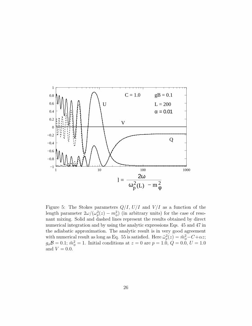
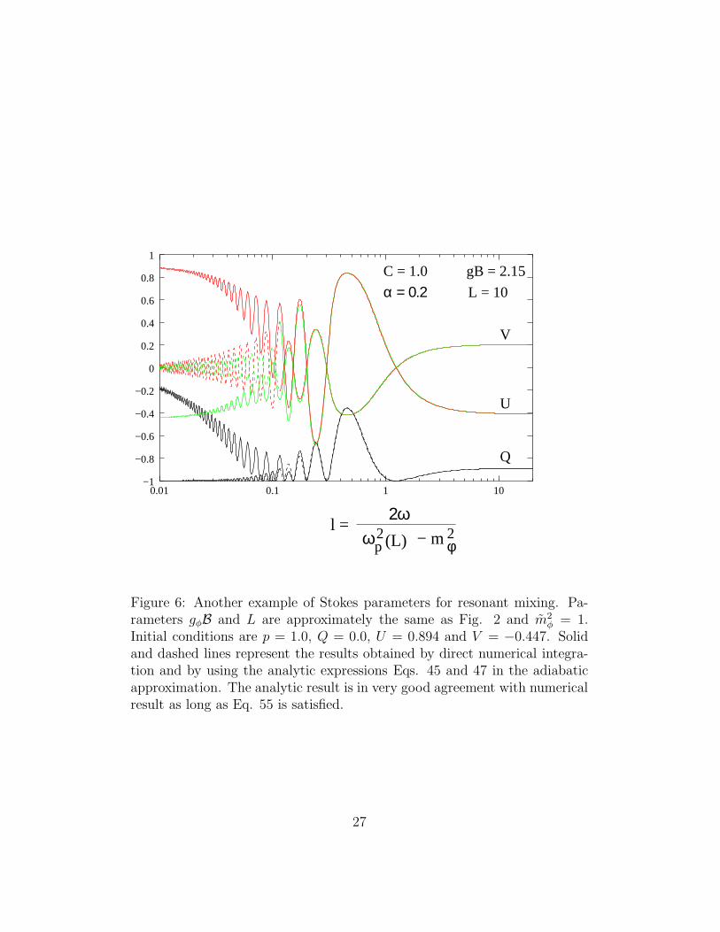
In fig. 5 and 6 we show two examples of the result expected in the caseof resonant mixing. Here the initial state of polarization has been chosenrandomly. The parameters values (in arbitrary units) given in the figuremay be translated to those relevant for cosmological propagation by takingthe units in the appropriate powers of Mpc. The pseudoscalar mass is chosensuch that m2

φ = m2φ/ω0 = 1, where ω0 is defined in Eq. 52. As expected,

observable effects are large at low frequencies compared to the correspondingresults of a uniform background. We also find rapid fluctuations in thisregion. The analytic result, obtained in the adiabatic limit, is found to bein good agreement with the numerical result as long as Eq. 55 is satisfied.

25

− m2φ

2ωl =

ω2p (L)

gB = 0.1C = 1.0

L = 200

α = 0.01

Q

U

V

−1

−0.8

−0.6

−0.4

−0.2

0

0.2

0.4

0.6

0.8

1

1 10 100 1000

Figure 5: The Stokes parameters Q/I, U/I and V/I as a function of thelength parameter 2ω/(ω2

p(z) −m2φ) (in arbitrary units) for the case of reso-

nant mixing. Solid and dashed lines represent the results obtained by directnumerical integration and by using the analytic expressions Eqs. 45 and 47 inthe adiabatic approximation. The analytic result is in very good agreementwith numerical result as long as Eq. 55 is satisfied. Here ω2

p(z) = m2φ−C+αz;

gφB = 0.1; m2φ = 1. Initial conditions at z = 0 are p = 1.0, Q = 0.0, U = 1.0

and V = 0.0.

26

− m2φ

2ωl =

ω2p (L)

gB = 2.15C = 1.0

L = 10

V

U

Q

α = 0.2

−1

−0.8

−0.6

−0.4

−0.2

0

0.2

0.4

0.6

0.8

1

0.01 0.1 1 10

Figure 6: Another example of Stokes parameters for resonant mixing. Pa-rameters gφB and L are approximately the same as Fig. 2 and m2

φ = 1.Initial conditions are p = 1.0, Q = 0.0, U = 0.894 and V = −0.447. Solidand dashed lines represent the results obtained by direct numerical integra-tion and by using the analytic expressions Eqs. 45 and 47 in the adiabaticapproximation. The analytic result is in very good agreement with numericalresult as long as Eq. 55 is satisfied.

27

At smaller frequencies the two results start to disagree. As expected, wenumerically find that the Stokes parameters approach their initial values inthe limit ω → 0.

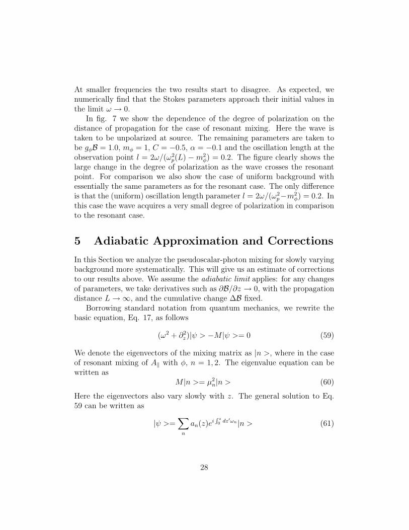
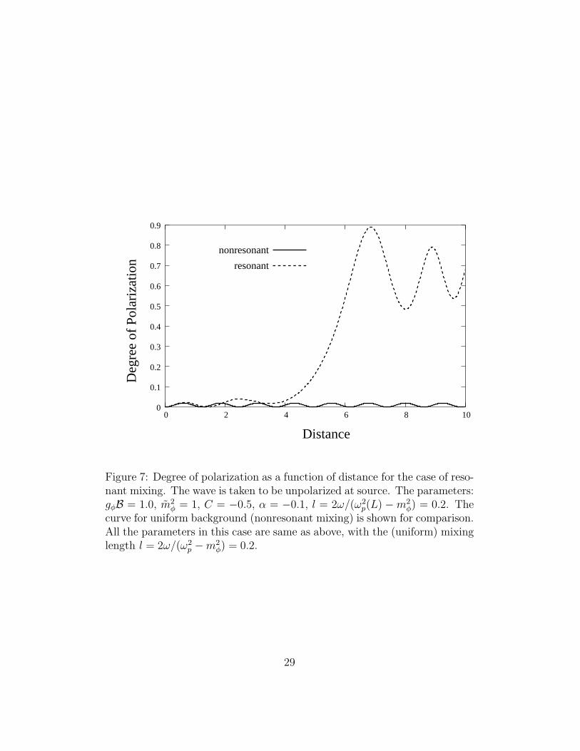
In fig. 7 we show the dependence of the degree of polarization on thedistance of propagation for the case of resonant mixing. Here the wave istaken to be unpolarized at source. The remaining parameters are taken tobe gφB = 1.0, mφ = 1, C = −0.5, α = −0.1 and the oscillation length at theobservation point l = 2ω/(ω2

p(L) −m2φ) = 0.2. The figure clearly shows the

large change in the degree of polarization as the wave crosses the resonantpoint. For comparison we also show the case of uniform background withessentially the same parameters as for the resonant case. The only differenceis that the (uniform) oscillation length parameter l = 2ω/(ω2

p−m2φ) = 0.2. In

this case the wave acquires a very small degree of polarization in comparisonto the resonant case.

5 Adiabatic Approximation and Corrections

In this Section we analyze the pseudoscalar-photon mixing for slowly varyingbackground more systematically. This will give us an estimate of correctionsto our results above. We assume the adiabatic limit applies: for any changesof parameters, we take derivatives such as ∂B/∂z → 0, with the propagationdistance L→ ∞, and the cumulative change ∆B fixed.

Borrowing standard notation from quantum mechanics, we rewrite thebasic equation, Eq. 17, as follows

(ω2 + ∂2z )|ψ > −M |ψ >= 0 (59)

We denote the eigenvectors of the mixing matrix as |n >, where in the caseof resonant mixing of A‖ with φ, n = 1, 2. The eigenvalue equation can bewritten as

M |n >= µ2n|n > (60)

Here the eigenvectors also vary slowly with z. The general solution to Eq.59 can be written as

|ψ >=∑

n

an(z)eiR z0

dz′ωn|n > (61)

28

Deg

ree

of P

olar

izat

ion

Distance

0

0.1

0.2

0.3

0.4

0.5

0.6

0.7

0.8

0.9

0 2 4 6 8 10

nonresonant

resonant

Figure 7: Degree of polarization as a function of distance for the case of reso-nant mixing. The wave is taken to be unpolarized at source. The parameters:gφB = 1.0, m2

φ = 1, C = −0.5, α = −0.1, l = 2ω/(ω2p(L) −m2

φ) = 0.2. Thecurve for uniform background (nonresonant mixing) is shown for comparison.All the parameters in this case are same as above, with the (uniform) mixinglength l = 2ω/(ω2

p −m2φ) = 0.2.

29

where ωn ≈ ω − µ2n

2ωSubstituting this into Eq. 59, and taking the overlap of

the resulting equation with < m| we find

∂zam = −1

2

∂zωm

ωmam − 1

ωm

∑

n

anωnei

R z0

dz′(ωn−ωm) < m|∂z|n > (62)

We have dropped all terms involving two derivatives of the slowly varyingquantities such as an(z), |n > and the exponent. Using the eigenvalue equa-tion, Eq. 60, we find

< m|∂z|n >=< m|(∂zM)|n >

µ2n − µ2

m

m 6= n (63)

The resulting solution for am can be written as

am(z) = e−1

2

R z0

dz′(∂z′ωm)/ωmbm(z) (64)

where bm(z) satisfies

∂zbm =1

ωm

∑

n,n 6=m

bnωn< m|(∂zM)|n >

µ2m − µ2

n

√

ωn(0)ωm(z)

ωn(z)ωm(0)ei

R z0

dz′(ωn−ωm) (65)

We pause to assess the result if we simply assumed bm(z) were constant.The pre-factor in Eq. 64 is integrated via

exp

(

−1

2

∫ z

0

dz′(∂z′ωm)/ωm

)

=

√

ωm(0)

ωm(z), (66)

which is the well-known WKB 1/√

k(z) factor cited earlier. In effect we havederived this factor and pushed the remaining derivatives in the equation forbm(z), Eq. 65. It is clear that this exponential term is approximately equalto one.

We note that the equation for bm is very similar for the equation 62 foran. This sets up an iterative scheme. Since slowly varying ωn ∼ ω, we canapproximate Eq. 65 as

∂zbm ≈∑

n,n 6=m

bn< m|(∂zM)|n >

µ2m − µ2

n

eiR z

0dz′(ωn−ωm) , (67)

30

plus small corrections in a series expansion of |ω − ωn|/ω << 1. For thecosmological applications, we consider here, the parameters ranges are suchthat the correction terms are extremely small.

The value of bm(L)− bm(0) gives an estimate of the transition amplitudebetween the two local eigenstates after the wave has propagated a distance L.Let us now estimate this with dimensional arguments. In the adiabatic limit,bn, as well as the term < m|(∂zM)|n > /(µ2

m − µ2n), varies slowly compared

to the exponential. Hence we may take these to be approximately constantalong the path. We can now integrate Eq. 67 to obtain the transition ampli-tude. We find that bm(L)− bm(0) is of order ω/(L∆µ2) as long as we ignorethe case of resonant mixing, where the two eigenmodes come very close toone another at some point along the path. Hence we find that in the limitL >> ω/∆µ2 the transition probability is negligible: this is the usual jus-tification for the adiabatic approximation when the internal dynamical timescale is very short compared to the time scale for changes of parameters.

5.0.1 Estimating the Transition Probability for Resonant Mixing

We turn to estimating the transition probability in the case of resonant mix-ing. We assume that the plasma frequency changes linearly along the pathaccording to the relation Eq. 52. We again take the direction of the back-ground magnetic field fixed so that we consider the two state mixing problem.In this case we find, for example,

∂zb2 = b1α

2

2gφBω[(C − αz)2 + (2gφBω)2]

e−iR z0

dz′

2ω(µ2

+−µ2−

) (68)

Now if we assume that the exponential is the most rapidly varying factor onthe right hand side of the above equation then we can replace the coefficientby its average value along the path. We then find,

b2(L) ≈ b2(0) + ib1(0)ω

L

[

tan−1m2

φ − ω2p(0)

2gφBω− tan−1

m2φ − ω2

p(L)

2gφBω

]

×(

e−iR L0

dz′(µ2+−µ2

−)/2ω

√

(m2φ − ω2

p(L))2 + (2gφBω)2

− 1√

(m2φ − ω2

p(0))2 + (2gφBω)2

)

(69)

31

where we have used[

2gφBω(m2

φ − ω2p(z))

2 + (2gφBω)2

]

av

=1

Lα

[

tan−1m2

φ − ω2p(0)

2gφBω− tan−1

m2φ − ω2

p(L)

2gφBω

]

It is clear that the second term on the right hand side of Eq. 69 is smalland hence the transition probability from one state to another is negligibleas long as L is sufficiently large such that

L >>ω

|µ2+ − µ2

−|. (70)

However this condition is not general and is applicable only in the limit oflarge ω. The basic problem is that close to the region where ωp = mφ, ouroriginal assumption that the coefficient of the exponential in the right handside of Eq. 68 varies slowly compared to the exponential term is not correct.We see this by comparing the magnitudes of the logarithmic derivatives ofthese two factors. We find

D1 =d

dzlog

[

(C − αz)2 + (2gφBω)2]

=−2α(C − αz)

(C − αz)2 + (2gφBω)2

D2 =d

dzlog e−i

R z0

dz′

2ω(µ2

+−µ2

−) =

1

2ω

√

(C − αz)2 + (2gφBω)2

The assumption, |D1| << |D2|, implies

|2α(C − αz)|(C − αz)2 + (2gφBω)2

<<1

2ω

√

(C − αz)2 + (2gφBω)2 (71)

In regions where |C − αz| >> 2gφBω this condition demands

|α| << 1

4ω(C − αz)2 .

Since (C − αz) is of order m2φ this condition implies

|α| << 1

4ωm2

φ .

We next consider the limit where |C − αz| is small or comparable to 2gφBω.We test the condition, Eq. 71, at the point |C − αz| = β(2gφBω). In thiscase we find

|α| << (β2 + 1)3/2

β(gφB)2ω

32

This condition is most stringent for very small values of β. However inthis region, as we show below, the transition probability between instanta-neous eigenstates continues to be very small provided the condition Eq. 70is obeyed. If we take β of order unity then this condition implies |α| <<(gφB)2ω, which can be expressed as,

L >>|ω2

p(L) − ω2p(0)|

(gφB)2ω, (72)

which is rather stringent for small frequencies and magnetic fields. In re-gions where this condition is violated we can no longer ignore the transitionbetween different instantaneous eigenstates.

We can obtain an estimate of the transition probability in regions whereEq. 71 is violated. Assume that in these regions the exponential term inEq. 68 varies much slowly compared to the coeffient. We then replace theexponential with its average over the path. We perform the integration overthe region where C−αz ranges from β(2gφBω) to −β(2gφBω). In this regionwe find

∆b2 = tan−1 β[

b2e−i

R z0

dz′

2ω(µ2

+−µ2−

)]

av(73)

The exponential term gives a contribution of order unity. It follows that thetransition probability between different eigenstates is non-negligible, unlessβ << 1.

Summary The above results can summarized by stating that in the caseof resonant mixing the adiabatic approximation is valid only if both theequations Eq. 70 and Eq. 72 are satisfied. If either of these equation is notrespected then the transition probability between instantaneous eigenstatescannot be ignored.

6 Applications

The basic aim of the present paper is to make detailed predictions for polar-ization observables due to pseudoscalar photon mixing, which can be testedin future astrophysical and cosmological observations. Tests may involveCMBR, polarization observations from distant sources, or propagation ofelectromagnetic waves through regions of strong magnetic fields such as thepulsar magnetosphere or Active Galactic Nuclei. The resonance phenomenon

33

may play an important role in many of these situations since the waves prop-agate through regions with large variations in plasma density. A detailedstudy of all this phenomenon is beyond the scope of the present paper. Herewe shall confine ourselves to simple estimates.

We first determine the range of frequencies for which the adiabaticitycondition is satisfied in the case of resonance in the supercluster magneticfields. Using equation 72, with B = 0.1 µG [20], ne = 10−6 cm−3, L = 10Mpc and the current limit on the coupling gφ = 6×10−11 GeV−1, we find thatadiabaticity is satisfied if ω >> 5 × 10−3 eV. Hence we expect a significanteffect at optical frequencies but negligible at radio. We should point outthat if resonance occurs it gives a considerably enhancement of the mixingphenomenon in comparison to the case of uniform background. For the latterthe mixing probability is limited by the oscillation length l in the medium andis proportional to (gBl)2 [15]. For low frequencies this is very small and givesa significant effect only if ω > 5 eV. On the other hand for a spatially varyingmedium if ωp = mφ somewhere along the path, the mixing probability is oforder unity as long as the adiabaticity constraint Eq. 72 is satisfied. Thisconstraint is satisfied at much smaller frequencies in comparison to what isrequired to obtain a significant effect if ωp 6= mφ all along the path.

For the galactic magnetic fields B ≈ 3 µG and plasma density ne ≈0.03 cm−3 and distance scale 50 Kpc, we find that adiabaticity condition issatisfied only for ω >> 50 eV. Hence here it is satisfied only for ultravioletfrequencies. Hence we can expect significant effects due to pseudoscalar-photon mixing at such high frequencies.

The effects of resonance are most dramatic if (gBl)2 << 1, where l is theoscillation length evaluated at some point far away from resonant region. Inthis case the resonant effects dominate. For supercluster magnetic fields thisis found to be the case for a wide range of frequencies 5 × 10−3 < ω < 1eV (here the lower limit is determined by the adiabaticity condition). Inthis case the results Eq. 51 apply and the wave becomes almost entirelylinearly polarized after crossing the resonant region, independent of its stateof polarization at origin. If the direction of the magnetic field remains fixedduring propagation then its state of polarization is well described by Eq. 51.In general, however, the magnetic field will also twist along the path. Inthis case the wave will also acquire circular polarization during propagation.This phenomenon is discussed in a separate paper [29]. If the frequency islarge, such that (gBl)2 >> 1, then the effect of pseudoscalar-photon mixingis large irrespective of whether resonance occurs or not.

34

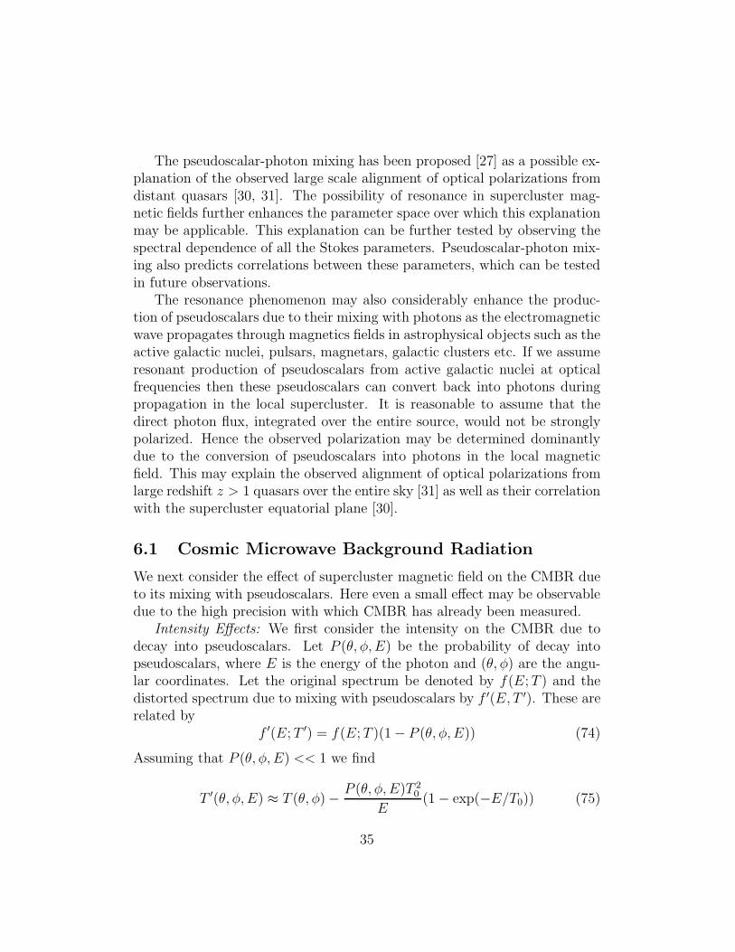
The pseudoscalar-photon mixing has been proposed [27] as a possible ex-planation of the observed large scale alignment of optical polarizations fromdistant quasars [30, 31]. The possibility of resonance in supercluster mag-netic fields further enhances the parameter space over which this explanationmay be applicable. This explanation can be further tested by observing thespectral dependence of all the Stokes parameters. Pseudoscalar-photon mix-ing also predicts correlations between these parameters, which can be testedin future observations.

The resonance phenomenon may also considerably enhance the produc-tion of pseudoscalars due to their mixing with photons as the electromagneticwave propagates through magnetics fields in astrophysical objects such as theactive galactic nuclei, pulsars, magnetars, galactic clusters etc. If we assumeresonant production of pseudoscalars from active galactic nuclei at opticalfrequencies then these pseudoscalars can convert back into photons duringpropagation in the local supercluster. It is reasonable to assume that thedirect photon flux, integrated over the entire source, would not be stronglypolarized. Hence the observed polarization may be determined dominantlydue to the conversion of pseudoscalars into photons in the local magneticfield. This may explain the observed alignment of optical polarizations fromlarge redshift z > 1 quasars over the entire sky [31] as well as their correlationwith the supercluster equatorial plane [30].

6.1 Cosmic Microwave Background Radiation

We next consider the effect of supercluster magnetic field on the CMBR dueto its mixing with pseudoscalars. Here even a small effect may be observabledue to the high precision with which CMBR has already been measured.

Intensity Effects: We first consider the intensity on the CMBR due todecay into pseudoscalars. Let P (θ, φ, E) be the probability of decay intopseudoscalars, where E is the energy of the photon and (θ, φ) are the angu-lar coordinates. Let the original spectrum be denoted by f(E;T ) and thedistorted spectrum due to mixing with pseudoscalars by f ′(E, T ′). These arerelated by

f ′(E;T ′) = f(E;T )(1 − P (θ, φ, E)) (74)

Assuming that P (θ, φ, E) << 1 we find

T ′(θ, φ, E) ≈ T (θ, φ) − P (θ, φ, E)T 20

E(1 − exp(−E/T0)) (75)

35

where T0 is the mean CMBR temperature. As expected mixing with pseu-doscalars will produce both a frequency and angular dependence of the tem-perature. To be consistent with observations we expect P (θ, φ, E) can havea maximum value of order 10−5.

Angular Distributions: It is interesting to speculate that the mixing withpseudoscalars in the local supercluster might give rise to prefered orientationof the CMBR quadrupole and octupole [32, 33] due to a possible angulardependence of the mixing probability. This may also explain why highermultipoles are aligned with the CMBR dipole [34]. “Cosmic variance”, in-voked to explain away magnitude puzzles, cannot credibly explain the mul-tiple coincidence of multipole directions. Hence an explanation in terms oflocal foreground effects is attractive. For consistency the mixing probabilityhas to be of order 10−5, which is roughly the strength of these multipole mo-ments. Current limits on the pseudoscalar photon coupling do not rule outthis possibility. However if local effects are the source, why should they be ofthe same order, multipole by multipole, as cosmological CMBR fluctuations?Interaction with a coherent pseudoscalar field might be the explanation withthe fewest number of arbitrary assumptions, although some fundamental re-vision of assumptions in cosmology might be needed to reconcile everythingobserved. Nevertheless it is interesting to investigate pseudoscalar-photonmixing in supercluster magnetic fields further since it may provide morestringent limits on the coupling gφ. Pseudoscalar-photon mixing will alsogive rise to a spectral dependence to the CMBR temperature. Hence the ef-fect has to be sufficiently small so that it does not conflict with the observedagreement [35] of CMBR with black body radiation formula.

Polarization: Pseudoscalar-photon mixing can also generate polarizationof the CMBR radiation. If the mixing probability is of order 10−5, which isrequired to explain the alignment of quadrupole and octupole, then it willgenerate polarization of the same order of magnitude. Hence if the polariza-tion is observed to be much smaller than this, it might be possible to imposefurther limits on the pseudoscalar photon coupling. The pseudoscalar-photonmixing can also change the CMBR polarization parameters without changingthe overall degree of polarization. This effect is in general much larger. How-ever if the degree of polarization of CMBR is small, as expected, any changein the polarization will be observable by the current detectors only if it is oforder unity. Hence here we require a relatively large contribution in order fornew effects to be observable. The shift in polarization is of the order of thephase acquired by the wave after propagating a distance L [27]. For uniform

36

medium this is of order (gφB)2lL, where l is the oscillation length. For theVirgo supercluster parameters and microwave frequencies of order 100 GHzwe find that the phase is of order 0.1 for the coupling gφ = 6× 10−11 GeV−1.This phase will generate all the Stokes parameters with relative strength oforder 0.1, assuming the current limit on the coupling gφ. Hence this contri-bution is small but it may be observable in future detectors. Similar resultsare found if we take into account the fluctuations in the plasma density [27]or propagation through intergalactic medium [17].

Condensate: A pseudoscalar condensate can also affect the CMB polar-ization [12]. In this case the rotation of polarization is equal to gφ∆φ, where∆φ is the total change of the pseudoscalar field along the trajectory of theelectromagnetic wave. This effect, however, cannot generate circular polar-ization. This effect is independent of frequency and will also affect radiowave polarizations from distant sources [27, 34]. If this pseudoscalar fielddistribution is anisotropic, it will lead to an anisotropy in both the CMB andradio polarizations [36]. Future observations can provide stringent limits onthis effect.

7 Dark Energy

Dark energy has come to denote a cosmic energy-momentum tensor of thevacuum. The source of dark energy is unknown. Unfortunately, the tradition-ally minimal option to employ one universal cosmological constant appearsless and less credible. It appears more likely that dark energy is the grav-itational trace of a field, somehow chaperoning the evolution of Big Bangpressures, densities and phase transitions predicted by particle physics [37].The need for a causal inflaton field is rather clearly manifested in the highuniformity of the cosmic microwave background (CMB) radiation.

By now, cosmology as a whole perhaps cannot do without a dark energy-associated field. Yet of all interactions, exploring the Universe with gravityhas a problem, in that gravity is the finest example where the coupling tofields is unknown! Unconventional as the remark may seem, in quantumtheory there exists no way to find independently that part of the energymomentum tensor which couples to gravity. The rules of coupling are un-known, and if at all knowable, appear to hinge on ultra-high energy physicsnot experimentally testable. The method of using gravity as a probe, whenit is not really known what gravity couples to, flies in the face of the long

37

successful tradition of using perturbatively stable interactions to study newsituations. It seems ironic that entire fields are built using gravity to explorethe Universe’s evolution when gravity is the least understood interaction.

If we assume that dark energy is associated with a scalar field φ, such afield will also have a coupling to electromagnetism given in Eq. 1. Hencethis field might produce all the physical effects we discuss in this paper.Couplings of dark energy to ordinary matter fields as well as their limitsare discussed by Carroll [19]. Yet the mass of such a conventional darkenergy field is expected to be of order 10−33 eV, and then much smaller thanthe intergalactic plasma frequency. Assuming such values we do not expectthe conditions for resonance to be applicable. One may, however, considergeneralized models of dark energy. Indeed it turns out that by invoking afalse vacuum it is possible to explain both dark matter and dark energy interms of the invisible axion [38, 39]. In this case the mass of the backgroundfield can be much larger than currently assumed. Hence we cannot rule outthe possibility that conditions for resonance may be applicable in some cases.

8 Summary

If one were to approach light and pseudoscalar field mixing “lightly,” thenthere is a sequence of facile, dimensionally based arguments that could beused. First, since gφ has dimensions of inverse mass, and electrodynamicsis a theory with no scale, one might claim that all effects were relativelyproportional to gφω, and must vanish for gφω << 1. This is false: the effectsare cumulative, and observable for exceedingly small gφ << 10−12 GeV−1.

Next one might observe that with a background field ~B, the effects must beof relative size gφB/ω, and vanish for large ω. This is again false, as thereare several other scales, sometimes ω occurs in the numerator, and we findthat for realistic parameters there are observable effects persisting all theway from radio to optical frequencies.

Then we return to our original goal of probing pseudoscalar field withlight. It is certainly very interesting that light can be dimmed by interac-tions with pseudoscalars. Yet in comparison the variety and variability ofpolarization-based observables seems almost unlimited. We believe that aspolarization observations accumulate, more and more anomalies will appear.It would be gratifying to have data so that a new and systematic study ofpseudoscalars via a coupling that is stable under perturbation theory can

38

commence.Acknowledgments: Work supported in part under Department of En-

ergy grant number DE-FG02-04ER41308.

References

[1] R. D. Peccei and H. Quinn, Phys. Rev. Lett. 38, 1440 (1977); Phys.

Rev. D 16, 1791 (1977).

[2] S. Weinberg, Phys. Rev. Lett. 40, 223 (1978); F. Wilczek, Phys. Rev.

Lett., 40, 279 (1978).

[3] M. Dine, W. Fischler and M. Srednicki, Phys. Lett., B 104, 199(1981).

[4] S. Kar, P. Majumdar, S. SenGupta and A. Sinha, Eur. Phys. J. C

23, 357 (2002); S. Kar, P. Majumdar, S. SenGupta and S. Sur, Class.

Quant. Grav. 19, 677 (2002); P. Majumdar and S. SenGupta, Class.

Quant. Grav. 16, L89 (1999).

[5] N. D. Hari Dass, K. V. Shajesh, Phys. Rev. D 65 085010 (2002),hep-th/0107006.

[6] A. Sen, Int. J. Mod. Phys. A 9, 3707 (1994).

[7] P. Das, P. Jain and S. Mukherjee, hep-ph/0011279, Int. Jour. of Mod.

Phys. A 16, 4011 (2001).

[8] S. Hannestad and L. Mersini-Houghton, hep-ph/0405218.

[9] J. N. Clarke, G. Karl and P.J.S. Watson, Can. J. Phys. 60, 1561(1982).

[10] P. Sikivie, Phys. Rev. Lett. 51, 1415 (1983); Phys. Rev. D 32, 2988(1985); P. Sikivie, Phys. Rev. Lett. 61, 783 (1988).

[11] L. Maiani, R. Petronzio and E. Zavattini, Phys. Lett. B175, 359(1986).

[12] D. Harari and P. Sikivie, Phys. Lett. B 289, 67 (1992).

39

[13] G. Raffelt and L. Stodolsky, Phys. Rev. D 37, 1237 (1988).

[14] R. Bradley et al, Rev. Mod. Phys. 75, 777 (2003).

[15] E. D. Carlson and W. D. Garretson, Phys. Lett. B 336,431 (1994).

[16] M. Yoshimura, Phys. Rev. D 37, 2039 (1988).

[17] C. Csaki, N. Kaloper, J. Terning, Phys. Rev. Lett. 88, 161302, (2002);Phys. Lett. B 535, 33, (2002).

[18] C. Deffayet, D. Harari, J. P. Uzan and M. Zaldarriaga, Phys. Rev. D

66, 043517 (2002); E. Mortsell, L. Bergstrom, A. Goobar, Phys. Rev.

D 66, 047702 (2002); M. Christensson and M. Fairbairn, Phys. Lett.

B 565, 10 (2003); Y. Grossman, S. Roy and J. Zupan, Phys. Lett. B

543, 23 (2002); E. Mortsell and A. Goobar JCAP 0304, 003 (2003).

[19] S. M. Carroll, Phys. Rev. Lett. 81, 3067 (1998)

[20] J. P. Vallee, The Astronomical Journal 99, 459 (1990); The Astro-

nomical Journal 124, 1322 (2002).

[21] for a recent review see, R. D. McKeown and P. Vogel Phys. Rept.

394, 315 (2004), hep-ph/0402025.

[22] The Review of Particle Physics, S. Eidelman et al Phys. Lett. B 592,1 (2004).

[23] L. J. Rosenberg and K. A. van Bibber, Phys. Rep. 325 1 (2000).

[24] G. G. Raffelt, Ann. Rev. Nucl. Part. Sci. 49, 163, (1999);hep-ph/9903472.

[25] J. W. Brockway, E. D. Carlson and G.G. Raffelt, Phys. Lett. B383,439 (1996), astro-ph/9605197; J. A. Grifols, E. Masso and R. Toldra,Phys. Rev. Lett. 77, 2372 (1996).

[26] M. Born and E. Wolf, Principles of Optics, (Pergamon Press, NewYork, 1989).

[27] P. Jain, S. Panda and S. Sarala, Phys. Rev. D 66, 085007 (2002),hep-ph/0206046.

40

[28] F. W. J. Olver, Asymptotics and Special Functions, Academic Press,(1974).

[29] S. Das, P. Jain, J. P. Ralston and R. Saha, hep-ph/0410006.

[30] D. Hutsemekers, 1998, Astronomy & Astrophysics, 332, 410 (1998);D. Hutsemekers and H. Lamy, Astronomy & Astrophysics, 367, 381(2001); R. A. Cabanac, D. Hutsemekers, D. Sluse and H. Lamy,astro-ph/0501043.

[31] P. Jain, G. Narain and S. Sarala, Mon. Not. Roy. Astron. Soc. 347,394 (2004), astro-ph/0301530.

[32] A. de Oliveira-Costa, M. Tegmark, M. Zaldarriaga and A. Hamilton,Phys. Rev. D 69, 063516 (2004), astro-ph/0307282.

[33] H. K. Eriksen et al, ApJ 605, 14 (2004), astro-ph/0307507.

[34] J. P. Ralston and P. Jain, Int. J. Mod. Phys. D 13, 1857 (2004),astro-ph/0311430,

[35] J.C. Mather et al., Astrophys. J. 420, 439 (1994).

[36] P. Jain and J. P. Ralston, Mod. Phys. Lett. A 14, 417 (1999).

[37] B. Ratra and P.J.E. Peebles, Phys. Rev. D 37, 3406 (1988); P.J.E.Peebles and B. Ratra, Astrophys. J. 325, L17 (1988).

[38] S. Barr and D. Seckel, Phys. Rev. D 64, 123513 (2001),hep-ph/0106239

[39] P. Jain, hep-ph/0411279, to appear in Mod. Phys. Lett. A.

41