probing liquid surface waves, liquid properties and liquid films with light diffraction
TRANSCRIPT
arX
iv:p
hysi
cs/0
5101
84v2
[ph
ysic
s.op
tics]
4 A
pr 2
006
Probing liquid surface waves, liquid properties and liquid films
with light diffraction
Tarun Kr. Barik, Partha Roy Chaudhuri, Anushree Roy and Sayan Kar∗
Department of Physics, Indian Institute of Technology, Kharagpur 721 302, India
Abstract
Surface waves on liquids act as a dynamical phase grating for incident light. In this article, we
revisit the classical method of probing such waves (wavelengths of the order of mm) as well as
inherent properties of liquids and liquid films on liquids, using optical diffraction. A combination
of simulation and experiment is proposed to trace out the surface wave profiles in various situations
(eg. for one or more vertical, slightly immersed, electrically driven exciters). Subsequently, the
surface tension and the spatial damping coefficient (related to viscosity) of a variety of liquids are
measured carefully in order to gauge the efficiency of measuring liquid properties using this optical
probe. The final set of results deal with liquid films where dispersion relations, surface and interface
modes, interfacial tension and related issues are investigated in some detail, both theoretically and
experimentally. On the whole, our observations and analysis seem to support the claim that this
simple, low–cost apparatus is capable of providing a wealth of information on liquids and liquid
surface waves in a non–destructive way.
PACS numbers: 42.25.Fx, 42.25.Hz,42.30.Kq,42.30.Lr,05.70.Np,68.05.-n
∗Electronic address: [email protected]
1
I. INTRODUCTION
Optical probes are usually non–destructive – they do not change the properties of the
medium being probed in any significant way (unless the probe power is large). Diffraction
and scattering of light, as is known over centuries, are therefore capable of providing a variety
of information. In this article, we revisit a well-known classical method of investigating
liquid surface waves using light diffraction. Although this method is well–studied in the
context of measurements of surface tension of liquids [1], our motivation for revisiting it is
primarily aimed at demonstrating its utility and capability in understanding a wider class
of situations/phenomena. In particular, we investigate two aspects – surface wave profiles
and liquid properties for waves on a single liquid and also for waves on liquid films.
Before we begin with details, it is worth summarizing some of the earlier work on liquid
as well as solid surface waves. Use of laser light scattering is a unique technique for non-
contact, noninvasive study of surface acoustic waves and capillary waves [2]. Technological
advances directed toward diverse applications of surface acoustic waves on solid surfaces
are now well established, and has resulted in important developments in the fabrication of
practical devices [3, 4, 5, 6, 7, 8, 9, 10, 11].
However, relatively few articles deal with surface waves on liquid surfaces [12, 13, 14,
15, 16, 17, 18, 19, 20]. To mention a few, high frequency capillary waves at the surface of
liquid gallium and the mercury liquid-vapor interface have been studied by means of quasi-
elastic light-scattering spectroscopy [21]. The spatial damping coefficient of low-frequency
surface waves at air-water interfaces, using a novel heterodyne light–scattering technique,
has been measured and reported in [22]. Quasi-elastic light scattering has been used to
study thermally excited capillary waves on free liquid surfaces over a considerably wider
range of surface wavenumbers [13, 16]. Measurements of the decay coefficient of capillary
waves in liquids covered with monolayers of stearic acid, oleyl alcohol, and hemicyanine
are reported in [23]. Also, the measurement of the pressure-area compression isotherm in
Langmuir monolayer films using the laser light diffraction from surface capillary waves is
reported in [24].
In a recent article, we have shown how the effect of interfering waves on a liquid surface
could be inferred from the nature of the diffraction pattern [15]. Here we begin by proposing
a combined method of simulation and experiment, sufficiently general in nature and capable
2
of verifying the nature of the actual liquid surface wave profile. Having known the profile,
we then focus on the dispersion relation and discuss experiments to determine the surface
tension and viscosity of liquids. Finally, we turn to liquid films where we try to understand
the profile through the various modes (surface and interface) and then go on to check the
values of interfacial tension.
Section II describes the basic scheme of our experimental arrangement. The methodology
of our experiment and typical results pertaining to the surface wave profile are discussed
in section III. In section IV, we discuss theory, observations and measurements of surface
tension and viscosity for different liquids. Section V first discusses the theoretical platform
for surface capillary wave on liquid films. We then verify our theory with experiments.
Finally, in section VI, we summarize our results with some concluding remarks.
II. EXPERIMENTAL DETAILS AND THE THEORETICAL BACKGROUND
A. Experimental setup
iθ
����������������������������
������
������
iB
F
A
D
C
E
FIG. 1: Schematic diagram of the experimental setup to study capillary wave on liquid; A: Laser,
B: Frequency generator, C: Screen, D: Loudspeaker, E: Spectrometer and prism table assembly
and F: Exciter.
As shown in Fig. 1, a petridish of diameter about 18.5 cm is filled with the experimental
liquid to a depth of ∼ 1 cm. A metal pin with its blunt end glued vertically upright to the
diaphragm of a loud speaker (held above the petridish) acts as an exciter. When slightly
immersed in the liquid and driven by a low frequency sinusoidal signal generator, this exciter
3
vibrates vertically up and down and generates the desired liquid surface waves. To study the
profile of surface waves we place the petridish-loud-speaker assembly on the prism-table of a
spectrometer in order to choose the diffracting element at any position on the liquid surface
and to record the corresponding position from the prism-table scale (with a least count of
0.1 degree). Light from a 5 mW He-Ne laser (λ = 632.8 nm) having a beam diameter of
∼ 1.8 mm is directed to fall on the liquid surface at an angle of incidence of 770 (θi), as
noted in our experiment. The laser beam incident on the dynamical phase grating formed
on the liquid surface, produces Fraunhofer diffraction pattern which is observed on a screen
placed at a fairly large distance (3.42 meters in our case) from the diffraction center. The
images of the diffraction pattern are recorded using a digital camera (make Sony, DSC -
P93, 5.1 mega pixels). Spurious noise in the image is removed using Photoshop software.
The intensity across the diffraction spots are measured using a photo-detector operating
in the linear dynamic range of the photo-currents’ response to optical power. During our
experiment, the room temperature recorded is 250C.
B. Theoretical background
We discuss here, briefly, the diffraction mechanism which lies at the heart of all our
experiments. When monochromatic light of wavelength λ is incident on a circular surface
wave of frequency ω and wavevector K, the phase modulation produced by the surface wave
is given as
φ(x′) =2π
λ
[
(2h cos θi) sin
(
ωt−Kx′
cos θi
)]
(1)
where, the factor of cos θi appears due to oblique incidence of the incident monochromatic
light [11, 14, 15, 25]. The field strength E of the diffraction pattern can be estimated from
the Fourier transform of the aperture function (in this case the surface wave produced by
single exciter). The intensity of the diffraction patterns, obtained from EE∗, is given by
[25, 26]
I(x′) =∑
n
J2n (4πh cos θi/λ) δ
(
x′
λz−
n
Λ cos θi
)
(2)
where z is the horizontal distance between the location of the laser spot on the liquid surface
and the screen and Λ = 2πK
, is the wavelength of the surface wave. h is the amplitude of the
surface wave. x′ is the coordinate which measures the distance of the diffraction spots from
a reference point (central spot) on the observation plane. Jn is the Bessel function of order
4
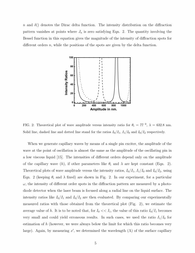
n and δ() denotes the Dirac delta function. The intensity distribution on the diffraction
pattern vanishes at points where Jn is zero satisfying Eqn. 2. The quantity involving the
Bessel function in this equation gives the magnitude of the intensity of diffraction spots for
different orders n, while the positions of the spots are given by the delta function.
0 200 400 600 800 10000
20
40
60
80
100
Inte
nsity
Rat
ios
Amplitude in nm.
FIG. 2: Theoretical plot of wave amplitude versus intensity ratio for θi = 77 0, λ = 632.8 nm.
Solid line, dashed line and dotted line stand for the ratios I0/I1, I1/I0 and I0/I2 respectively.
When we generate capillary waves by means of a single pin exciter, the amplitude of the
wave at the point of oscillation is almost the same as the amplitude of the oscillating pin in
a low viscous liquid [15]. The intensities of different orders depend only on the amplitude
of the capillary wave (h), if other parameters like θi and λ are kept constant (Eqn. 2).
Theoretical plots of wave amplitude versus the intensity ratios, I0/I1, I1/I0 and I0/I2, using
Eqn. 2 (keeping θi and λ fixed) are shown in Fig. 2. In our experiment, for a particular
ω, the intensity of different order spots in the diffraction pattern are measured by a photo-
diode detector when the laser beam is focused along a radial line on the liquid surface. The
intensity ratios like I0/I1 and I0/I2 are then evaluated. By comparing our experimentally
measured ratios with those obtained from the theoretical plot (Fig. 2), we estimate the
average value of h. It is to be noted that, for I0 << I1, the value of this ratio I0/I1 becomes
very small and could yield erroneous results. In such cases, we used the ratio I1/I0 for
estimation of h (however, we were always below the limit for which this ratio becomes very
large). Again, by measuring x′, we determined the wavelength (Λ) of the surface capillary
5
waves to be 2.1 mm [for more details see [15]]. For several exciters placed at different types
of geometric configurations (eg, along a line, or a polygon etc.), the surface wave patterns
change, and hence Eqn. 2 must also change.
III. THE SURFACE WAVE PROFILE
A. Simulation of the profile
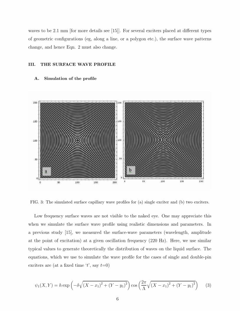
FIG. 3: The simulated surface capillary wave profiles for (a) single exciter and (b) two exciters.
Low frequency surface waves are not visible to the naked eye. One may appreciate this
when we simulate the surface wave profile using realistic dimensions and parameters. In
a previous study [15], we measured the surface-wave parameters (wavelength, amplitude
at the point of excitation) at a given oscillation frequency (220 Hz). Here, we use similar
typical values to generate theoretically the distribution of waves on the liquid surface. The
equations, which we use to simulate the wave profile for the cases of single and double-pin
exciters are (at a fixed time ‘t’, say t=0)
ψ1(X, Y ) = h exp(
−δ√
(X − x1)2 + (Y − y1)
2)
cos(
2π
Λ
√
(X − x1)2 + (Y − y1)
2)
(3)
6
and
ψ2(X, Y ) = h exp(
−δ√
(X − x1)2 + (Y − y1)
2)
cos(
2π
Λ
√
(X − x1)2 + (Y − y1)
2)
+
h exp(
−δ√
(X − x2)2 + (Y − y2)
2)
cos(
2π
Λ
√
(X − x2)2 + (Y − y2)
2)
, (4)
respectively. Here (x1, y1) and (x2, y2) are the centers of oscillations and δ is the spatial
damping coefficient of the liquid. To mimic the intended experiments, we assume that each
wave has the same frequency ω, wavelength Λ, and amplitude h (at the center of oscillation).
In our simulations, we use the typical values of Λ = 2.1 mm, h =1.0 mm and D = 8.4 mm
(separation between pin-exciters) [15]. δ is chosen to be 0.235 cm−1 (for water at 220 Hz,
we obtain this value from experiments discussed later in section IV). The corresponding
surface-wave profiles estimated for the two cases of interest are shown in Fig. 3(a) and
Fig. 3(b), respectively. Following this recipe one can obtain the surface-wave profile for any
number of oscillation sources. The simulated profiles enable a better visualization, which,
in turn, can act as a guideline for their actual experimental verification.
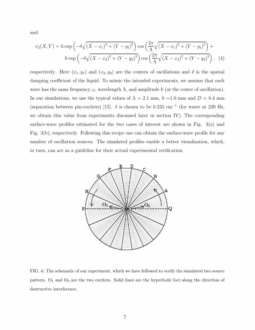
FIG. 4: The schematic of our experiment, which we have followed to verify the simulated two source
pattern. O1 and O2 are the two exciters. Solid lines are the hyperbolic loci along the direction of
destructive interference.
7
B. Experimental results for two source pattern
The simulated profiles are built on the assumptions made in Eqn. 3 and Eqn. 4. It is
necessary to verify experimentally whether the assumptions are good enough to represent
the characteristics of the surface waves. We note that the simulated two source interference
pattern [shown in Fig. 3(b)] exhibits hyperbolic loci for the constructive and destructive
interference nodes. Using this fact as a guideline, we trace the hyperbolic loci (maxima
and minima of the interfering waves) on the liquid surface by observing the changes in
the corresponding diffraction patterns. Initially, when the laser beam is incident along the
central line PQ (see Fig. 4) where constructive interference of waves occur, the diffracted
light shows, as expected [15], a central spot along with higher order ones symmetrically
located on either side of the central spot [see Fig. 5(a)]. As we shift the probe beam
gradually away from the central line along a circle (note the arrow in Fig. 4), the number of
higher order spots progressively decreases till we reach the position of the adjacent hyperbola
(O2A), where the diffraction should ideally contain only the central order. In experiment,
however, at this position, we find the first order spots too, though with very low intensity
[see Fig. 5(b)]. This happens due to the finite spot size of the laser beam. Nevertheless,
beginning with the central line at one side and gradually rotating the prism-table till we reach
1800, we observe a repetition of the patterns [shown in Fig. 5(a) and 5(b)] symmetrically
at all complementary angles. We note the angular positions of all consecutive minima.
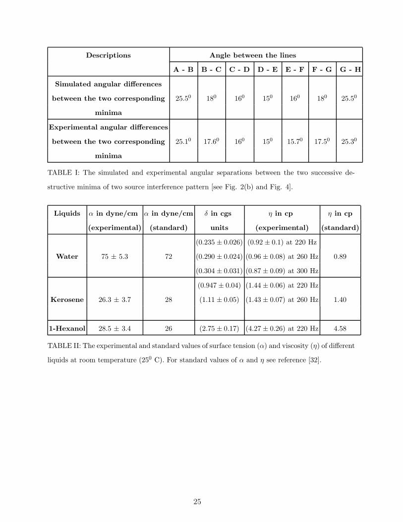
These results are shown in Table-I. Thus, a comparison of our experiment (Fig. 4) with the
simulation [upper half of Fig. 3(b)] for identical values of parameters shows the same number
(eight) of destructive interference lines at almost the same angular separation. Beyond 1800
and upto 3600, (i.e, while scanning the lower semicircular region in Fig. 4) identical patterns
are observed. This confirms that the Eqn. 4 used to describe and simulate the two source
surface wave profile is, indeed, a correct representation of the observed profile. We note that
our method of investigation is sufficiently general (we have indeed checked upto six exciters)
and can be used for several exciters located along a line or in other geometric configurations
(eg. exciters on a triangle, quadrilateral, pentagon, hexagon etc.).
8
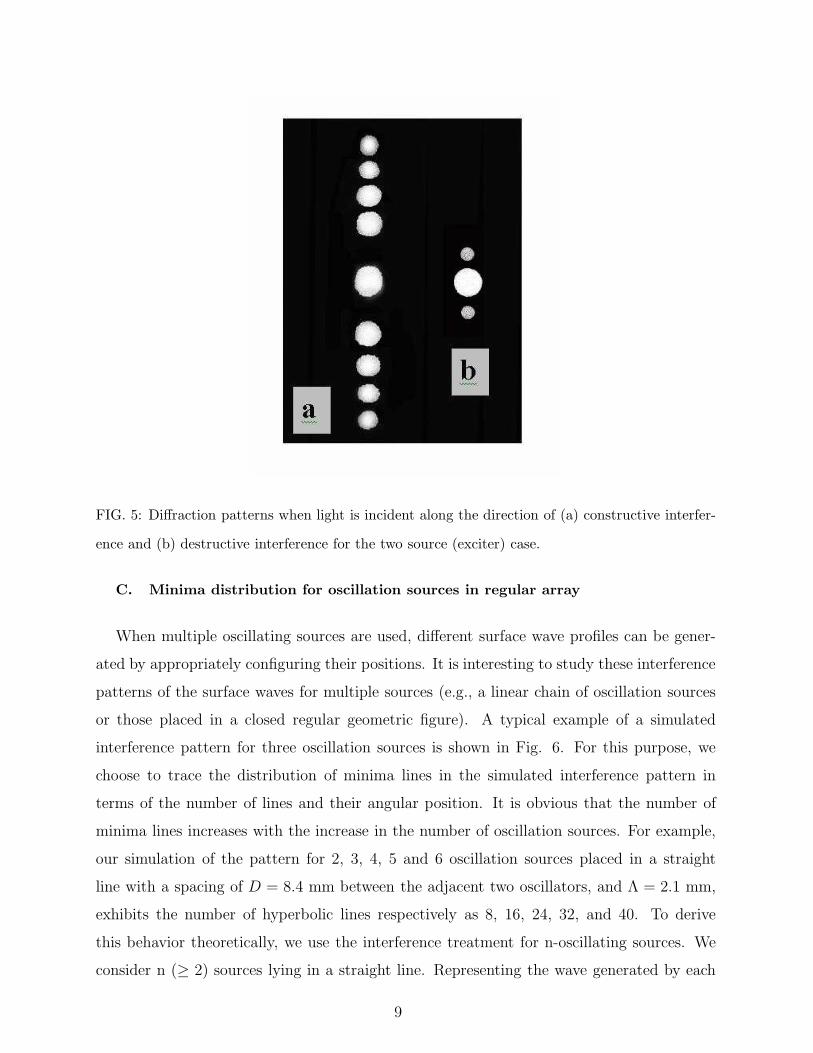
FIG. 5: Diffraction patterns when light is incident along the direction of (a) constructive interfer-
ence and (b) destructive interference for the two source (exciter) case.
C. Minima distribution for oscillation sources in regular array
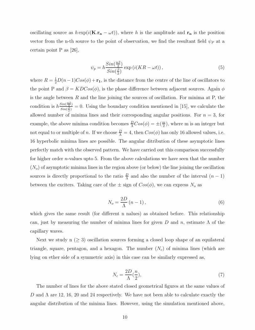
When multiple oscillating sources are used, different surface wave profiles can be gener-
ated by appropriately configuring their positions. It is interesting to study these interference
patterns of the surface waves for multiple sources (e.g., a linear chain of oscillation sources
or those placed in a closed regular geometric figure). A typical example of a simulated
interference pattern for three oscillation sources is shown in Fig. 6. For this purpose, we
choose to trace the distribution of minima lines in the simulated interference pattern in
terms of the number of lines and their angular position. It is obvious that the number of
minima lines increases with the increase in the number of oscillation sources. For example,
our simulation of the pattern for 2, 3, 4, 5 and 6 oscillation sources placed in a straight
line with a spacing of D = 8.4 mm between the adjacent two oscillators, and Λ = 2.1 mm,
exhibits the number of hyperbolic lines respectively as 8, 16, 24, 32, and 40. To derive
this behavior theoretically, we use the interference treatment for n-oscillating sources. We
consider n (≥ 2) sources lying in a straight line. Representing the wave generated by each
9
oscillating source as h exp(i(K.rn − ωt)), where h is the amplitude and rn is the position
vector from the n-th source to the point of observation, we find the resultant field ψP at a
certain point P as [26],
ψp = hSin(nβ
2)
Sin(β
2)
exp (i(KR− ωt)) , (5)
where R = 12D(n−1)Cos(φ)+ r1, is the distance from the centre of the line of oscillators to
the point P and β = KDCos(φ), is the phase difference between adjacent sources. Again φ
is the angle between R and the line joining the sources of oscillation. For minima at P, the
condition is hSin(nβ
2)
Sin(β
2)
= 0. Using the boundary condition mentioned in [15], we calculate the
allowed number of minima lines and their corresponding angular positions. For n = 3, for
example, the above minima condition becomes DΛCos(φ) = ±(m
2), where m is an integer but
not equal to or multiple of n. If we choose DΛ
= 4, then Cos(φ) has only 16 allowed values, i.e.
16 hyperbolic minima lines are possible. The angular ditribution of these asymptotic lines
perfectly match with the observed pattern. We have carried out this comparison successfully
for higher order n-values upto 5. From the above calculations we have seen that the number
(No) of asymptotic minima lines in the region above (or below) the line joining the oscillation
sources is directly proportional to the ratio DΛ
and also the number of the interval (n − 1)
between the exciters. Taking care of the ± sign of Cos(φ), we can express No as
No =2D
Λ(n− 1) , (6)
which gives the same result (for different n nalues) as obtained before. This relationship
can, just by measuring the number of minima lines for given D and n, estimate Λ of the
capillary waves.
Next we study n (≥ 3) oscillation sources forming a closed loop shape of an equilateral
triangle, square, pentagon, and a hexagon. The number (Nc) of minima lines (which are
lying on ether side of a symmetric axis) in this case can be similarly expressed as,
Nc =2D
Λ(n
2), (7)
The number of lines for the above stated closed geometrical figures at the same values of
D and Λ are 12, 16, 20 and 24 respectively. We have not been able to calculate exactly the
angular distribution of the minima lines. However, using the simulation mentioned above,
10
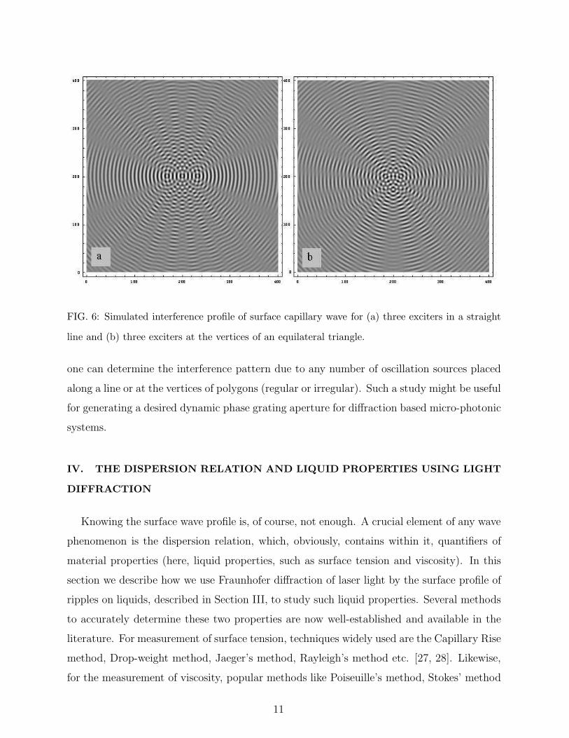
FIG. 6: Simulated interference profile of surface capillary wave for (a) three exciters in a straight
line and (b) three exciters at the vertices of an equilateral triangle.
one can determine the interference pattern due to any number of oscillation sources placed
along a line or at the vertices of polygons (regular or irregular). Such a study might be useful
for generating a desired dynamic phase grating aperture for diffraction based micro-photonic
systems.
IV. THE DISPERSION RELATION AND LIQUID PROPERTIES USING LIGHT
DIFFRACTION
Knowing the surface wave profile is, of course, not enough. A crucial element of any wave
phenomenon is the dispersion relation, which, obviously, contains within it, quantifiers of
material properties (here, liquid properties, such as surface tension and viscosity). In this
section we describe how we use Fraunhofer diffraction of laser light by the surface profile of
ripples on liquids, described in Section III, to study such liquid properties. Several methods
to accurately determine these two properties are now well-established and available in the
literature. For measurement of surface tension, techniques widely used are the Capillary Rise
method, Drop-weight method, Jaeger’s method, Rayleigh’s method etc. [27, 28]. Likewise,
for the measurement of viscosity, popular methods like Poiseuille’s method, Stokes’ method
11
0+1+2
−2−1
hx z
l
d
θΛ
ExciterIncident light
FIG. 7: Geometrical representation of the basic measurement on surface tension and viscosity.
etc., are well-known and gives accurate results [27, 28]. Here, we focus on a single optical
set up which can measure both surface tension and viscosity of low-viscous liquids with
reasonable accuracy. Though the measurement of surface tension of liquids using Fraunhofer
diffraction of laser light by surface waves is well known in the literature [1], to the best of
our knowledge the estimation of the viscosity of a liquid using this probe and, in particular,
the simple method which we have followed, is certainly new. In the following we elaborate
on the above mentioned measurements in some detail.
A. Surface tension
Consider the well-known dispersion relation for surface capillary wave on liquids [29, 30,
31]
ω2 =(
gK + αK3/ρ)
. (8)
Here ω and K are the angular frequency and wavevector of the surface capillary wave,
respectively. α and ρ are the surface tension and density of the liquid and g is the acceleration
due to gravity. The above relation shows that waves at the surface of the liquid are dominated
by gravity as well as surface tension. Neglecting the gravitational effect and taking the
logarithm on both sides of the Eqn. 8 we get
lnω =3
2lnK +
1
2ln
(
α
ρ
)
, (9)
which is an equation of a straight line for lnω vs. lnK with a slope of 32
and y-intercept
12ln(
αρ
)
, which contains the surface tension α.
In our experiments, we have generated the surface capillary wave on the liquid surface
with a single exciter. As we discussed before, the expected surface wave profile [shown in
Fig. 3(a)] acts as a reflection phase grating for the incident laser light and the intensity
12
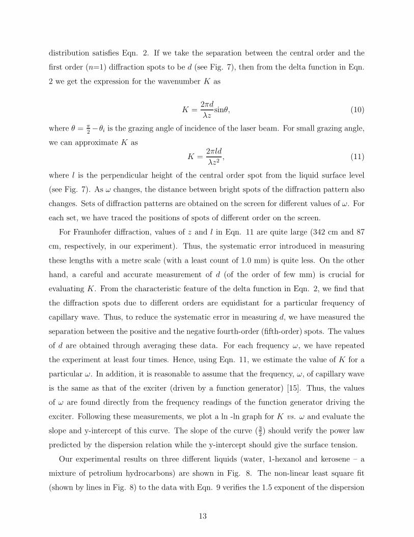
distribution satisfies Eqn. 2. If we take the separation between the central order and the
first order (n=1) diffraction spots to be d (see Fig. 7), then from the delta function in Eqn.
2 we get the expression for the wavenumber K as
K =2πd
λzsinθ, (10)
where θ = π2−θi is the grazing angle of incidence of the laser beam. For small grazing angle,
we can approximate K as
K =2πld
λz2, (11)
where l is the perpendicular height of the central order spot from the liquid surface level
(see Fig. 7). As ω changes, the distance between bright spots of the diffraction pattern also
changes. Sets of diffraction patterns are obtained on the screen for different values of ω. For
each set, we have traced the positions of spots of different order on the screen.
For Fraunhofer diffraction, values of z and l in Eqn. 11 are quite large (342 cm and 87
cm, respectively, in our experiment). Thus, the systematic error introduced in measuring
these lengths with a metre scale (with a least count of 1.0 mm) is quite less. On the other
hand, a careful and accurate measurement of d (of the order of few mm) is crucial for
evaluating K. From the characteristic feature of the delta function in Eqn. 2, we find that
the diffraction spots due to different orders are equidistant for a particular frequency of
capillary wave. Thus, to reduce the systematic error in measuring d, we have measured the
separation between the positive and the negative fourth-order (fifth-order) spots. The values
of d are obtained through averaging these data. For each frequency ω, we have repeated
the experiment at least four times. Hence, using Eqn. 11, we estimate the value of K for a
particular ω. In addition, it is reasonable to assume that the frequency, ω, of capillary wave
is the same as that of the exciter (driven by a function generator) [15]. Thus, the values
of ω are found directly from the frequency readings of the function generator driving the
exciter. Following these measurements, we plot a ln -ln graph for K vs. ω and evaluate the
slope and y-intercept of this curve. The slope of the curve (32) should verify the power law
predicted by the dispersion relation while the y-intercept should give the surface tension.
Our experimental results on three different liquids (water, 1-hexanol and kerosene – a
mixture of petrolium hydrocarbons) are shown in Fig. 8. The non-linear least square fit
(shown by lines in Fig. 8) to the data with Eqn. 9 verifies the 1.5 exponent of the dispersion
13
0.0 0.1 0.21.8
2.0
2.2
2.4
6.0
6.5
7.0
7.5
8.0
8.5
3.0 3.5 4.0 4.5
Y-intercept
Kerosene
ln
1-Hexanol
ln K
Water
FIG. 8: The ln-ln plots of the wavevector (K) versus the frequency (ω) exhibit a straight line
of slope very close to 32 obtained for three different liquids. The inset shows the corresponding
y-intercepts.
relation within experimental uncertainty (1.5±0.03). Using the known value of ρ for each
liquid, we estimate the value of α from the measured y-intercept of the straight lines. It is
to be noted that the maximum percentage error in measuring α is limited to 6% - 8% (for
different liquids) by our measurement procedure. We have tabulated the measured values
of surface tension for different liquids in Table-II. These results match quite well with the
standard values of surface tension for the corresponding liquids [32].
B. Viscosity
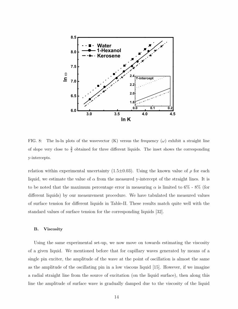
Using the same experimental set-up, we now move on towards estimating the viscosity
of a given liquid. We mentioned before that for capillary waves generated by means of a
single pin exciter, the amplitude of the wave at the point of oscillation is almost the same
as the amplitude of the oscillating pin in a low viscous liquid [15]. However, if we imagine
a radial straight line from the source of excitation (on the liquid surface), then along this
line the amplitude of surface wave is gradually damped due to the viscosity of the liquid
14
10 20 30 400
200
400
600
800Frequency 220 Hz
Ampl
itude
in n
m
Distance (x) in mm
FIG. 9: Experimental plot of distance (x) versus surface capillary wave amplitude (h). Solid line,
dashed line, and dotted line for the liquids water, kerosene, and 1-hexanol respectively.
(see Fig. 7). The laser beam is focused along a radial line at different distances on the
liquid surface from the point of excitation (x in Fig. 7). We have seen in Sec. II that the
intensities of the diffraction spots of different orders depend only on the amplitude of the
capillary wave, if other parameters like θi and λ are kept constant (Eqn. 2). By comparing
our experimentally measured intensity ratios of different orders in the diffraction pattern
with those obtained from the theoretical plot (Fig. 2), we estimate the average value of h
at a particular location on the liquid surface. In Fig. 9, we plot x, the distance from the
point of oscillation vs. h, the capillary wave amplitude for three experimental liquids (water,
kerosene, and 1-hexanol). We fit the data points with an exponential decay function, where
we kept the decay constant (also known as spatial damping coefficient of the liquid), δ, as
varying parameter. The values of δ for three different liquids are tabulated in Table-II.
The wavevector for a wave of fixed real frequency, ω, has a small imaginary part, which
contributes to the spatial damping. Substituting K = K0 + iδ (where δ << K0) in the well-
known Navier-Stokes equation for waves on a liquid-air interface, one gets[22, 33],
δ =4ηω
3α, (12)
where η is the viscosity of the liquid. Experimentally, we have obtained the values of α and
δ for the above mentioned liquids. The estimated value of viscosity of different liquids, using
Eqn. 12, are shown in Table-II. The experimental plots in Fig. 9 are for frequency 220 Hz.
15
We have also checked our results for two other frequencies (260 Hz and 300 Hz) and have
obtained similar results (see Table-II).
V. LIQUID FILMS ON LIQUIDS: THEORY AND EXPERIMENTS
Till now we have been exclusively concerned with waves on the surface of a single liquid,
or, more precisely, waves at the liquid-air interface. A more complicated scenario arises
when there exists a film of a different liquid on top of a given liquid (the two liquids are
immiscible). In such a situation, the dispersion relation changes drastically, which, in turn,
changes the surface wave profile. We now investigate the novelties that arise through studies
with our optical probe.
A. Background theoretical framework
The dispersion relation in Eqn. 8 for capillary wave propagation on liquid surfaces is
valid only when the depth of experimental liquid is large. For lower values of the depth of
the liquid (denoted by, say y), the relation becomes [30]
ω2 =αK3
ρtanh (Ky) (13)
where, here too, we neglect a term due to gravity. Typically, if we choose y = 1 cm and a
range of K from 20 to 80 cm −1 (as used in our earlier experiment), tanh (Ky) is nearly unity,
and the dispersion relation reduces to the one given by Eqn. 8. The interesting problem we
focus on now is that of wave propagation on a liquid film spread out on another liquid. If the
thickness of the film is very low, then not only the surface tension but also the interfacial
tension across the liquid-film boundary, play a role in the propagation mechanism of the
waves. We first work out a general dispersion relation where the surface and interfacial
tensions as well as the film thickness appear explicitly in our mathematical expressions.
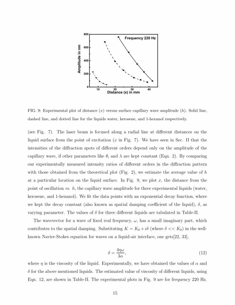
Fig. 10 shows the symbols used to represent various parameters in the following discus-
sion. We denote the density of the lower liquid by ρ while α is the interfacial tension at the
liquid-liquid interface. The same quantities for the film-air interface are represented with
primes i.e., ρ′
and α′
respectively. The equilibrium plane of separation (interface) between
the liquids is at y = 0. The liquid below the y = 0 plane extends upto a value y = −H
16
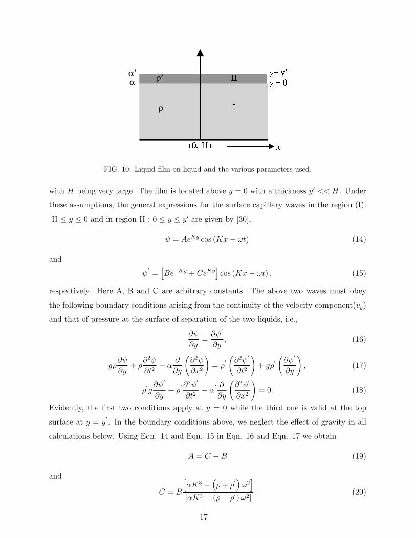
FIG. 10: Liquid film on liquid and the various parameters used.
with H being very large. The film is located above y = 0 with a thickness y′ << H. Under
these assumptions, the general expressions for the surface capillary waves in the region (I):
-H ≤ y ≤ 0 and in region II : 0 ≤ y ≤ y′ are given by [30],
ψ = AeKy cos (Kx− ωt) (14)
and
ψ′
=[
Be−Ky + CeKy]
cos (Kx− ωt) , (15)
respectively. Here A, B and C are arbitrary constants. The above two waves must obey
the following boundary conditions arising from the continuity of the velocity component(vy)
and that of pressure at the surface of separation of the two liquids, i.e.,
∂ψ
∂y=∂ψ
′
∂y, (16)
gρ∂ψ
∂y+ ρ
∂2ψ
∂t2− α
∂
∂y
(
∂2ψ
∂x2
)
= ρ′
(
∂2ψ′
∂t2
)
+ gρ′
(
∂ψ′
∂y
)
, (17)
ρ′
g∂ψ
′
∂y+ ρ
′ ∂2ψ′
∂t2− α
′ ∂
∂y
(
∂2ψ′
∂x2
)
= 0. (18)
Evidently, the first two conditions apply at y = 0 while the third one is valid at the top
surface at y = y′
. In the boundary conditions above, we neglect the effect of gravity in all
calculations below. Using Eqn. 14 and Eqn. 15 in Eqn. 16 and Eqn. 17 we obtain
A = C − B (19)
and
C = B
[
αK3 −(
ρ+ ρ′
)
ω2]
[αK3 − (ρ− ρ′)ω2]. (20)
17
Substituting Eqn. 19 and Eqn. 20 in Eqn. 18 with y = y′
, we construct a quadratic equation
for ω2 given by:
ω4[
1 + r tanh(
Ky′)]
− ω2[
ω2s tanh
(
Ky′)
+ rω2s + ω2
i
]
+ ω2sω
2i tanh
(
Ky′)
= 0, (21)
where, we have used the notations ρ′
ρ= r, α
′
K3
ρ′ = ω2
s and αK3
ρ= ω2
i for simplicity. The two
roots of Eqn. 21 are the new dispersion relations for our given problem. The two roots are
ω2±
=P ±
√G
2Q, (22)
where, P = rω2s + ω2
s tanh(
Ky′
)
+ ω2i , Q = 1 + r tanh
(
Ky′
)
, and G = P 2 −
4Qω2sω
2i tanh
(
Ky′
)
.
Consider two limiting cases of the above dispersion relation. Let us first assume y′ → ∞.
Then ω2+ → ω2
s and ω2−→ ω2
i
1+r= αK3
ρ+ρ′ . Thus, when y′ is very large, the ω+ mode corresponds
to the waves propagating on the upper liquid surface (thus called surface mode). On the
other hand, the ω− mode involves the interfacial tension [30] as well as the density of the
lower liquid and may be termed as an interface mode. In such a situation (y′ large), reflecting
the probe laser beam off the surface wave profile on the liquid film, we can obtain information
(through the diffraction pattern) on wave propagation and properties of the liquid film. The
existence of the other mode can be confirmed (for y′ large) only if we perform experiments
in transmitted light, though it is not clear how such information may be obtained. On
the contrary, assuming y′ → 0 (very thin film), we get ω2
+ → (rω2s + ω2
i ) =
(
α′
+α
)
K3
ρ, and
ω2−→ 0. Thus the ω+ mode now depends on properties of both the liquids, (α′, ρ), as well
as properties of the interface (α).
Furthermore, we can obtain the constants A, B, C and hence ψ and ψ′
by assuming a
value for the amplitude imparted initially at the top surface. In this way, one may obtain
the amplitudes of ψ and ψ′
for both the modes ω+ and ω−. In particular, we have noted (not
demonstrated here) that the nature of variation of the amplitudes of ψ′
(with the film-hight
0 < y′ < h) for the ω+ mode is quite different from that for the ω− mode. In the former case
(ω+) the value of the amplitude drops to a much smaller value at the interface compared to
the drop in the amplitude for the ω− mode. However, it is not possible for us to check this
fact through our experiments. Hence we refrain from discussing this aspect further in this
article.
18
B. Experiments and results
0 40 800
1
2
3
4
0 40 800
1
2
3
4
0 40 800
1
2
3
4
(a)
Water - o-xyline filmthickness = 0.158 cm
(x10
3 )
(b)
Water - o-xyline filmthickness = 0.016 cm
K
(c)
Water - o-xyline filmthickness = 0.032 cm
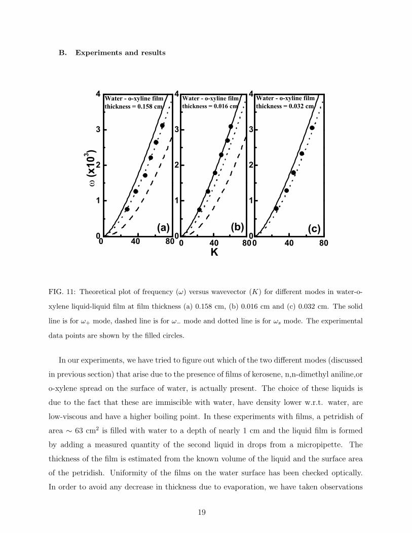
FIG. 11: Theoretical plot of frequency (ω) versus wavevector (K) for different modes in water-o-
xylene liquid-liquid film at film thickness (a) 0.158 cm, (b) 0.016 cm and (c) 0.032 cm. The solid
line is for ω+ mode, dashed line is for ω− mode and dotted line is for ωs mode. The experimental
data points are shown by the filled circles.
In our experiments, we have tried to figure out which of the two different modes (discussed
in previous section) that arise due to the presence of films of kerosene, n,n-dimethyl aniline,or
o-xylene spread on the surface of water, is actually present. The choice of these liquids is
due to the fact that these are immiscible with water, have density lower w.r.t. water, are
low-viscous and have a higher boiling point. In these experiments with films, a petridish of
area ∼ 63 cm2 is filled with water to a depth of nearly 1 cm and the liquid film is formed
by adding a measured quantity of the second liquid in drops from a micropipette. The
thickness of the film is estimated from the known volume of the liquid and the surface area
of the petridish. Uniformity of the films on the water surface has been checked optically.
In order to avoid any decrease in thickness due to evaporation, we have taken observations
19
within 5 minutes of the formation of the uniformly spread film. The measurements are of
the same type as those mentioned while studying surface tension (discussed in the earlier
section) except that, in the present case, we do the experiments for varying film thicknesses.
Here, we show our experimental results only for o-xylene films of different thicknesses on
water. For films of the other liquids mentioned above, on water, we have observed similar
behavior.
To find out the mode which is present on the film surface for a liquid-film of o-xylene on
water, we first plot the experimental ω ∼ K behavior with film thickness as a parameter.
The theoretically obtained ω-K curves for different modes : ω+, ω−, and ωs (as a limiting
case of ω+ mode) - are then placed on the same graph for comparison. Here we use standard
values : α = 37.2 dyne/cm, α′ = 29.8 dyne/cm, ρ′= 0.88 gm/cc, and ρ=1 gm/cc in Eqn.
22 [32]. It is evident that for a film of thickness as low as 0.016 cm, the measured data
corresponds to ω+ mode [Fig. 11(b)], while for films of thickness typically 0.158 cm, the
experimental data matches well with the ωs mode [Fig. 11(a)]. However, any intermediate
thickness between 0.016 and 0.158 cm yields data within the ω+ and ωs modes [Fig. 11(c)].
This clearly shows that the ω+ mode always dominates over ω− mode. For thicker films the
ω+ mode coincides with ωs mode, whereas for thinner films the mode is still ω+, though it
is modified by the presence of the interfacial tension and the density of the lower liquid and
is not equal to ωs.
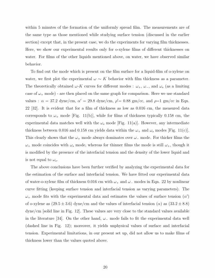
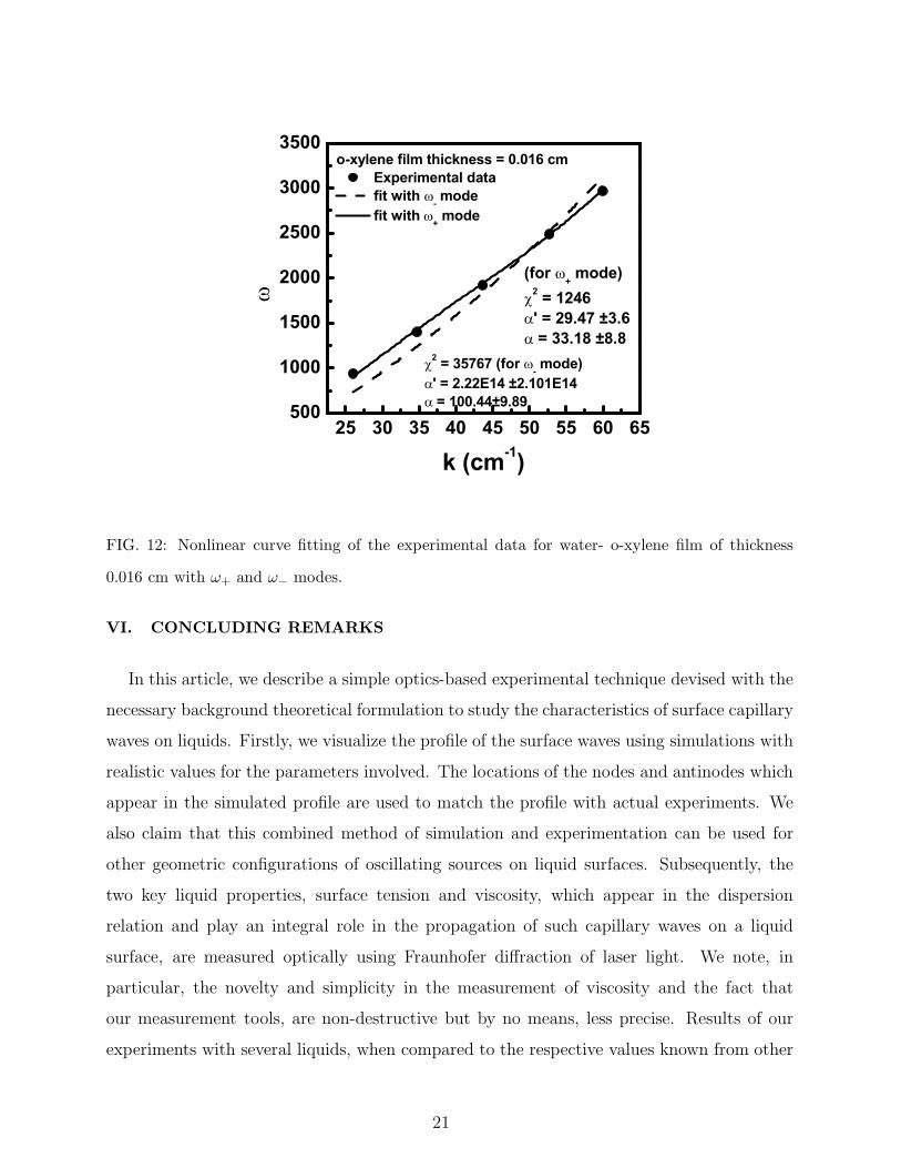
The above conclusions have been further verified by analyzing the experimental data for
the estimation of the surface and interfacial tension. We have fitted our experimental data
of water-o-xylene film of thickness 0.016 cm with ω+ and ω− modes in Eqn. 22 by nonlinear
curve fitting (keeping surface tension and interfacial tension as varying parameters). The
ω+ mode fits with the experimental data and estimates the values of surface tension (α′)
of o-xylene as (29.5 ± 3.6) dyne/cm and the values of interfacial tension (α) as (33.2 ± 8.8)
dyne/cm [solid line in Fig. 12]. These values are very close to the standard values available
in the literature [34]. On the other hand, ω− mode fails to fit the experimental data well
(dashed line in Fig. 12); moreover, it yields unphysical values of surface and interfacial
tension. Experimental limitations, in our present set up, did not allow us to make films of
thickness lower than the values quoted above.
20
25 30 35 40 45 50 55 60 65500
1000
1500
2000
2500
3000
3500
o-xylene film thickness = 0.016 cm Experimental data fit with - mode fit with + mode
2 = 35767 (for - mode)' = 2.22E14 ±2.101E14 = 100.44±9.89
(for + mode)2 = 1246' = 29.47 ±3.6 = 33.18 ±8.8
k (cm-1)
FIG. 12: Nonlinear curve fitting of the experimental data for water- o-xylene film of thickness
0.016 cm with ω+ and ω− modes.
VI. CONCLUDING REMARKS
In this article, we describe a simple optics-based experimental technique devised with the
necessary background theoretical formulation to study the characteristics of surface capillary
waves on liquids. Firstly, we visualize the profile of the surface waves using simulations with
realistic values for the parameters involved. The locations of the nodes and antinodes which
appear in the simulated profile are used to match the profile with actual experiments. We
also claim that this combined method of simulation and experimentation can be used for
other geometric configurations of oscillating sources on liquid surfaces. Subsequently, the
two key liquid properties, surface tension and viscosity, which appear in the dispersion
relation and play an integral role in the propagation of such capillary waves on a liquid
surface, are measured optically using Fraunhofer diffraction of laser light. We note, in
particular, the novelty and simplicity in the measurement of viscosity and the fact that
our measurement tools, are non-destructive but by no means, less precise. Results of our
experiments with several liquids, when compared to the respective values known from other
21
sources and literature, summarily establish the efficacy and accuracy of our approach. We
anticipate, in future, the introduction of technological sophistications in our set-up, which
might lead to an ‘Optical Surfacetensometer cum Viscometer’. The advantage of having a
single set-up for measuring both these properties need not be further emphasised. Finally, we
investigate, both experimentally and theoretically, an interesting aspect of capillary wave
characteristics involved with a liquid film placed on the surface of an immissible liquid.
The dispersion relation we frame to study this case not only explains the features of the
surface and interfacial modes, but also provides an estimate of the interfacial tension across
the film-liquid boundary. In summary, our experimental and theoretical results seem to
demonstrate the capability of our set-up in carrying out studies pertaining to capillary wave
profile, liquid properties and waves on liquid films on liquids. Despite its limitations, the
wide variety of information which can be obtained from such a simple set-up, makes it a
tool worth improving upon in future investigations.
VII. ACKNOWLEDGMENT
Anushree Roy and Tarun Kumar Barik thank Department of Science and Technology
(DST), New Delhi, India, for financial support. TKB also thanks Dibyendu Chowdhury,
an undergraduate student of Vidyasagar University, West Bengal, India, for his help while
doing some of the experiments.
[1] G. Weisbuch and F. Garbay,“Light scattering by surface tension waves”, Am. J. Phys. 47,
355-356 (1979).
[2] E. Wolf (ed), Progress in Optics, Vol. XI, (North-Holland publishing company - Amsterdam,
London, 1973), pp. 125-165.
[3] D.P. Morgan, “A history of surface acoustic wave devices”, Int. jou. of high speed electronics
and systems 10, 553-602 (2000); and the references therein.
[4] A. Khan, R. Rimeika, D. Ciplys, R. Gaska and M.S. Shur, “Optical guided modes and surface
acoustic waves in GaN grown on (0001) sapphire substrats”, Phys. Status Solidi B 216, 477-
480 (1999) .
22
[5] C.S. Tsai, ”Integrated acoustooptic circuits and applications”, IEEE Trans. Ultrson. Fer-
roeletr. Freq.Control 39, 529-554 (1992); and the references therein.
[6] C. Deger, E. Born, H. Angerer, O. Ambacher, M. Stutzmann, J. Hornsteine, E. Riha and
G. Fischeraurer, “Sound velocity of AlxGa1−xN thin films obtained by surface acuostic wave
measurements”, Appl. Phys. Lett. 72, 2400-2402 (1998).
[7] R. Rimeika, D. Ciplys, R. Gaska, J.W. Yang, M.A. Khan, M.S. Shur and E. Towe, ”Diffraction
of optical waves by surface acoustic waves in GaN”, Appl. Phys. Lett. 77(4), 480-482 (2000).
[8] P. A. Hess, ” Surface acoustic waves in materials science”, Physics Today, March, 42-47 (2002);
and the references therein.
[9] G.I. Stegeman, “Optical probing of surface waves and surface wave devices”, IEEE tran. on
sonic and ultrasonics su-23, 33-63 (1976); and the references therein.
[10] J.P. Monchalin, “Optical detection of ultrasound”, IEEE Trans. Ultrason. Ferroelectr. Freq.
Control 33, 485-498 (1986).
[11] B.D. Duncan, “ Visualization of surface acoustic waves by means of synchronous amplitude-
modulated illumination”, Appl. Opt. 39, 2888-2895 (2000) .
[12] F.R. Watson ”Surface Tension at the Interface of Two Liquids Determined Experimen-
tally by the Method of Ripple Waves”, Phys. Rev. 12, 257-278 (1901); F.R. Watson and
W.A.Shewhart, ”A study of ripple wave motion”,Phys. Rev. 7, 226-231 (1916) .
[13] J.C. Earnshaw and R.C. McGivren, “Photon correlation spectroscopy of thermal fluctuations
of liquid surface”, J.Phys.D 20, 82-92 (1987); J. C. Earnshaw and E. McCoo, “Mode mixing
of liquid surface waves”, Phys. Rev. Lett.72, 84-87 (1994).
[14] R. Miao, Z. Yang, J. Zhu and C. Shen, “Visualization of low frequency liquid surface acoustic
waves by means of optical diffraction”, Appl. Phys. Lett. 80, 3033-3035 (2002).
[15] T.K. Barik, A. Roy, S. Kar, “ A simple experiment on diffraction of light by interfering liquid
surface waves”, Am. J. Phys. 73 (8), 725-729 (2005).
[16] W.M. Klipstein, J.S. Radnich and S.K. Lamoreaux, “Thermally excited liquid surface waves
and their study through the quasielastic scattering of light”, Am. J. Phys. 64(6), 758-765
(1996).
[17] D. Walkenhorst, “Determining surface tension by light scattering”, (1999), Online(28/06/05):
//www.wooster. edu/physics/JrIS/Files/Walkenhorst.pdf.
[18] P.G. Klemens, “Dispersion relations for waves on liquid surface”, Am. J. Phys. 52, 451-452
23
(1984).
[19] D Langevin (ed.) Light scattering by liquid surfaces and complementary techniques (Marcel
Dekker, New York, 1992).
[20] I. B. Ivanov (ed.) Thin Liquid Films, Fundamentals and Applications, (Marcel Dekker Inc.,
Newyork, 1988), pp. 497-662.
[21] V. Kolevzon and G. Gerbeth, “Light scattering spectroscopy of a liquid gallium surface”, J.
Phys. D 29, 2071-2081 (1996); V. Kolevzon, G. Gerbeth and G. Pozdniakov, “Light-scattering
study of the mercury liquid-vapor interface”, Phys. Rev. E 55, 3134-3142, (1997).
[22] K.Y. Lee, T. Chou, D.S. Chung and E. Mazur, “Direct measurement of the spatial damping
of capillary waves at liquid-vapour interfaces”, J. Phys. Chem. 97, 12876-12878 (1993).
[23] J.R. Saylor, A.J. Szeri and G.P. Foulks, “Measurement of surfactant properties using a circular
capillary wave field”, Experiments in Fluids 29, 509-518 (2000).
[24] A. S. Martin, S. J. Lawrence, D. A. Rollett and J. R. Sambles, “Measurement of a Lang-
muir monomolecular film pressure- area compression isotherm using laser light diffracted from
surface capillary waves”, Eur. J. Phys.14, 19-22, (1993).
[25] J.W. Goodman, Introduction to Fourier optics, (McGrew-Hill, San Francisco, 1968), p.62.
[26] E. Hecht, Optics, 4th Ed. (Pearson Education ) 2003, pp. 449-450.
[27] L.I. Osipow, Surface Chemistry, (Reinhold publishing corporation, London), 7-21 (1993).
[28] S.K. Ghosh, A Text Book of Advanced Practical Physics, (New Central Book Agency, Calcutta,
1985), pp. 62-106.
[29] V.G. Levich, Physicochemical hydrodynamics, (Prentice-Hall Inc., 1962) p-596.
[30] L.D. Landau and E.M. Lifshitz, Fluid Mechanics, (Pergamon press, Oxford,1975), pp. 1-44,
230-241.
[31] L.E. Kinsler, A.R. Frey, A.B. Coppens and J.V. Sanders, Fundamentals of acoustics, 3rd Ed.
(Wiley, New york, 1982) pp. 141-162.
[32] D. R. Lide, Handbook of chemistry and physics, (CRC press , Newyork, 1998) pp. 6 14-170.
[33] J.A. Taylor, G.M. Lancaster and J.W. Rablais, Appl. Surf. Sci. 1, 503, 1978.
[34] D.L. Lord, K.F. Hayes, A.H. Demond and A. Salehzadeh, ”Influence of organic acid solution
chemistry on subsurface transport properties. 1. surface and interfacial tension”, Environ. Sci.
Technol. 31, 2045-2051 (1997).
24
Descriptions Angle between the lines
A - B B - C C - D D - E E - F F - G G - H
Simulated angular differences
between the two corresponding 25.50 180 160 150 160 180 25.50
minima
Experimental angular differences
between the two corresponding 25.10 17.60 160 150 15.70 17.50 25.30
minima
TABLE I: The simulated and experimental angular separations between the two successive de-
structive minima of two source interference pattern [see Fig. 2(b) and Fig. 4].
Liquids α in dyne/cm α in dyne/cm δ in cgs η in cp η in cp
(experimental) (standard) units (experimental) (standard)
(0.235 ± 0.026) (0.92 ± 0.1) at 220 Hz
Water 75 ± 5.3 72 (0.290 ± 0.024) (0.96 ± 0.08) at 260 Hz 0.89
(0.304 ± 0.031) (0.87 ± 0.09) at 300 Hz
(0.947 ± 0.04) (1.44 ± 0.06) at 220 Hz
Kerosene 26.3 ± 3.7 28 (1.11 ± 0.05) (1.43 ± 0.07) at 260 Hz 1.40
1-Hexanol 28.5 ± 3.4 26 (2.75 ± 0.17) (4.27 ± 0.26) at 220 Hz 4.58
TABLE II: The experimental and standard values of surface tension (α) and viscosity (η) of different
liquids at room temperature (250 C). For standard values of α and η see reference [32].
25