Probing Physics Beyond Standard Model with

Atomic and Molecular Phenomena

University of New South Wales

Hoang Bao Tran TanSupervisors: V. V. Flambaum and J. B. Berengut

April 22, 2021

Abstract

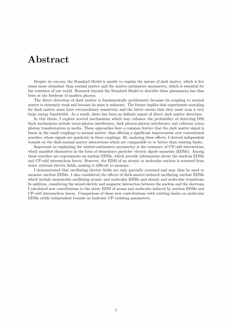
Despite its success, the Standard Model is unable to explain the nature of dark matter, which is fivetimes more abundant than normal matter and the matter-antimatter asymmetry, which is essential forthe existence of our world. Research beyond the Standard Model to describe these phenomena has thusbeen at the forefront of modern physics.

The direct detection of dark matter is fundamentally problematic because its coupling to normalmatter is extremely weak and because its mass is unknown. The former implies that experiments searchingfor dark matter must have extraordinary sensitivity and the latter means that they must scan a verylarge energy bandwidth. As a result, there has been no definite report of direct dark matter detection.

In this thesis, I explore several mechanisms which may enhance the probability of detecting DM.Such mechanisms include axion-photon interference, dark photon-photon interference and coherent axion-photon transformation in media. These approaches have a common feature that the dark matter signal islinear in the small couplings to normal matter, thus offering a significant improvement over conventionalsearches, whose signals are quadratic in these couplings. By analysing these effects, I derived independentbounds on the dark-normal matter interactions which are comparable to or better than existing limits.

Important to explaining the matter-antimatter asymmetry is the existence of CP-odd interactions,which manifest themselves in the form of elementary particles’ electric dipole moments (EDMs). Amongthese searches are experiments on nuclear EDMs, which provide information about the nucleon EDMsand CP-odd internucleon forces. However, the EDM of an atomic or molecular nucleus is screened fromstatic external electric fields, making it difficult to measure.

I demonstrated that oscillating electric fields are only partially screened and may thus be used tomeasure nuclear EDMs. I also considered the effects of dark-matter-induced oscillating nuclear EDMswhich include measurable oscillating atomic and molecular EDMs and atomic and molecular transitions.In addition, considering the mixed electric and magnetic interaction between the nucleus and the electrons,I calculated new contributions to the static EDM of atoms and molecules induced by nucleon EDMs andCP-odd internucleon forces. Comparison of these new contributions with existing limits on molecularEDMs yields independent bounds on hadronic CP-violating parameters.

1

List of publications

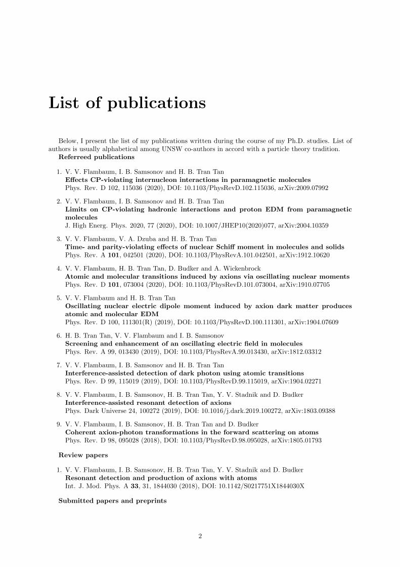
Below, I present the list of my publications written during the course of my Ph.D. studies. List ofauthors is usually alphabetical among UNSW co-authors in accord with a particle theory tradition.

Referreed publications

1. V. V. Flambaum, I. B. Samsonov and H. B. Tran TanEffects CP-violating internucleon interactions in paramagnetic moleculesPhys. Rev. D 102, 115036 (2020), DOI: 10.1103/PhysRevD.102.115036, arXiv:2009.07992

2. V. V. Flambaum, I. B. Samsonov and H. B. Tran TanLimits on CP-violating hadronic interactions and proton EDM from paramagneticmoleculesJ. High Energ. Phys. 2020, 77 (2020), DOI: 10.1007/JHEP10(2020)077, arXiv:2004.10359

3. V. V. Flambaum, V. A. Dzuba and H. B. Tran TanTime- and parity-violating effects of nuclear Schiff moment in molecules and solidsPhys. Rev. A 101, 042501 (2020), DOI: 10.1103/PhysRevA.101.042501, arXiv:1912.10620

4. V. V. Flambaum, H. B. Tran Tan, D. Budker and A. WickenbrockAtomic and molecular transitions induced by axions via oscillating nuclear momentsPhys. Rev. D 101, 073004 (2020), DOI: 10.1103/PhysRevD.101.073004, arXiv:1910.07705

5. V. V. Flambaum and H. B. Tran TanOscillating nuclear electric dipole moment induced by axion dark matter producesatomic and molecular EDMPhys. Rev. D 100, 111301(R) (2019), DOI: 10.1103/PhysRevD.100.111301, arXiv:1904.07609

6. H. B. Tran Tan, V. V. Flambaum and I. B. SamsonovScreening and enhancement of an oscillating electric field in moleculesPhys. Rev. A 99, 013430 (2019), DOI: 10.1103/PhysRevA.99.013430, arXiv:1812.03312

7. V. V. Flambaum, I. B. Samsonov and H. B. Tran TanInterference-assisted detection of dark photon using atomic transitionsPhys. Rev. D 99, 115019 (2019), DOI: 10.1103/PhysRevD.99.115019, arXiv:1904.02271

8. V. V. Flambaum, I. B. Samsonov, H. B. Tran Tan, Y. V. Stadnik and D. BudkerInterference-assisted resonant detection of axionsPhys. Dark Universe 24, 100272 (2019), DOI: 10.1016/j.dark.2019.100272, arXiv:1803.09388

9. V. V. Flambaum, I. B. Samsonov, H. B. Tran Tan and D. BudkerCoherent axion-photon transformations in the forward scattering on atomsPhys. Rev. D 98, 095028 (2018), DOI: 10.1103/PhysRevD.98.095028, arXiv:1805.01793

Review papers

1. V. V. Flambaum, I. B. Samsonov, H. B. Tran Tan, Y. V. Stadnik and D. BudkerResonant detection and production of axions with atomsInt. J. Mod. Phys. A 33, 31, 1844030 (2018), DOI: 10.1142/S0217751X1844030X

Submitted papers and preprints

2

1. V. V. Flambaum, I. B. Samsonov, H. B. Tran Tan and A. V. ViatkinaNuclear polarization effects in atoms and ionsSubmitted to Phys. Rev. A, January 2021

2. H. B. Tran Tan, V. V. Flambaum and J. C. BerengutDark Matter near gravitating bodiesarXiv:1808.01856v1

3

List of presentations

Below I present the list of my presentation at international and national conferences, workshops andcompetitions during the course of my Ph.D. studies.

1. Searching for Axions and Axionic Dark Matter with Interference and Axion-inducedNuclear Moments, TeV Particle Astrophysics Conference, University of Sydney, Sydney, Australia,December 2019

2. Screening and Enhancement of Nuclear Electric Dipole Moments Induced by AxionicDark Matter, Frontiers in Quantum Matter Workshop: Electric Dipole Moments, AustralianNational University, Canberra, Australia, November 2019

3. Effects of Dark Matter in atomic and molecular phenomena, Australian Institute of PhysicsPostgraduate Presentation Competition, University of Technology Sydney, Sydney, Australia,October 2019

4. Coherent axion-photon transformations in the forward scattering on atoms, QuantumTechnologies for Axion Dark Matter Detection Incubator, University of Sydney, Sydney, Australia,September 2018

5. Detection of Axions Using Atomic Transitions Induced by Interference between Elec-tromagnetic and Axion Fields, Australian Institute of Physics Summer Meeting, University ofNew South Wales, Sydney, Australia, December 2017

4

Acknowledgements

As I was writing the last sentences of my thesis, a realization started to come to me that anotherimportant stage of my life was drawing to its end and that I was about to leave the institution where Ihave stayed for more than seven years. Such a moment inevitably engenders certain emotional ambiguityand personal ambivalence. While I was honoured by the cause of my departure, I was saddened by thefact of it. While I was excited about the new horizon that had just appeared to me, I still wanted tospend more time among the people whom I have held so dear.

In particular, I was saddened by having to leave the tutelage of a teacher without parallel in myexperience. To me, Prof. Victor Flambaum has been a constant source of immeasurable knowledge,profound wisdom and everlasting inspiration. Above all, he is a true leader who knows instinctively whatto do and how to achieve it. I am deeply grateful to him for imparting to me his knowledge and his wayof thinking.

I would also like to thank my co-supervisor Prof Julian Berengut for his support, availability andconstructive suggestions, which were determinant for the accomplishment of the work presented in thisthesis.

I thank all of my co-authors, with whom I have worked on many interesting problems: Dmitry Budker,Vladimir Dzuba, Igor Samsonov, Yevgeny Stadnik and Arne Wickenbrock. Igor Samsonov is especiallyacknowledged for very fruitful collaborations, numerous comments and discussions and comprehensivesupport during my study. I am also grateful to Oleg Sushkov for many useful discussions and for his kindinterest in my research.

5

Contents

1 Introduction 101.1 Axion as a Dark Matter candidate . . . . . . . . . . . . . . . . . . . . . . . . . . . . . . . 10

1.1.1 The strong CP problem and the axion . . . . . . . . . . . . . . . . . . . . . . . . . 101.1.2 The axion as a DM Candidate . . . . . . . . . . . . . . . . . . . . . . . . . . . . . 11

1.2 Elementary particles’ EDMs and the solution to the matter-antimatter asymmetry . . . . 121.2.1 CP -violation and elementary particles’ EDMs . . . . . . . . . . . . . . . . . . . . . 121.2.2 Schiff’s theorem and methods to circumvent it . . . . . . . . . . . . . . . . . . . . 12

2 Interference-assisted resonant detection of axions 152.1 Overview . . . . . . . . . . . . . . . . . . . . . . . . . . . . . . . . . . . . . . . . . . . . . 152.2 Abstract . . . . . . . . . . . . . . . . . . . . . . . . . . . . . . . . . . . . . . . . . . . . . . 152.3 Introduction . . . . . . . . . . . . . . . . . . . . . . . . . . . . . . . . . . . . . . . . . . . . 162.4 Experimental scheme . . . . . . . . . . . . . . . . . . . . . . . . . . . . . . . . . . . . . . . 17

2.4.1 General set-up . . . . . . . . . . . . . . . . . . . . . . . . . . . . . . . . . . . . . . 172.4.2 Atomic transition . . . . . . . . . . . . . . . . . . . . . . . . . . . . . . . . . . . . . 18

2.5 Calculations . . . . . . . . . . . . . . . . . . . . . . . . . . . . . . . . . . . . . . . . . . . . 192.5.1 Photon-to-axion conversion probability . . . . . . . . . . . . . . . . . . . . . . . . . 192.5.2 Atomic transition amplitudes . . . . . . . . . . . . . . . . . . . . . . . . . . . . . . 192.5.3 Axion signal and signal-to-noise ratio . . . . . . . . . . . . . . . . . . . . . . . . . 20

2.6 Numerical estimates . . . . . . . . . . . . . . . . . . . . . . . . . . . . . . . . . . . . . . . 222.6.1 The M1 case - vapor target . . . . . . . . . . . . . . . . . . . . . . . . . . . . . . . 222.6.2 The M1 case - solid target . . . . . . . . . . . . . . . . . . . . . . . . . . . . . . . 222.6.3 Comparison of projected sensitivities . . . . . . . . . . . . . . . . . . . . . . . . . . 23

2.7 Conclusions . . . . . . . . . . . . . . . . . . . . . . . . . . . . . . . . . . . . . . . . . . . . 252.A Axion-photon interference with atomic transitions of M0 type . . . . . . . . . . . . . . . . 25

2.A.1 Scheme description . . . . . . . . . . . . . . . . . . . . . . . . . . . . . . . . . . . . 252.A.2 Calculations for the M0 case . . . . . . . . . . . . . . . . . . . . . . . . . . . . . . 262.A.3 Comparison with the M1 case . . . . . . . . . . . . . . . . . . . . . . . . . . . . . 282.A.4 Numerical estimates for the M0 case . . . . . . . . . . . . . . . . . . . . . . . . . . 28

2.B Axion laser . . . . . . . . . . . . . . . . . . . . . . . . . . . . . . . . . . . . . . . . . . . . 28

3 Coherent axion-photon transformations in the forward scattering on atoms 353.1 Overview . . . . . . . . . . . . . . . . . . . . . . . . . . . . . . . . . . . . . . . . . . . . . 353.2 Abstract . . . . . . . . . . . . . . . . . . . . . . . . . . . . . . . . . . . . . . . . . . . . . . 353.3 Introduction . . . . . . . . . . . . . . . . . . . . . . . . . . . . . . . . . . . . . . . . . . . . 353.4 Calculations . . . . . . . . . . . . . . . . . . . . . . . . . . . . . . . . . . . . . . . . . . . . 363.5 Numerical estimates . . . . . . . . . . . . . . . . . . . . . . . . . . . . . . . . . . . . . . . 37

3.5.1 Effective magnetic field in liquid xenon . . . . . . . . . . . . . . . . . . . . . . . . . 383.5.2 Effective electric field in vapor thallium . . . . . . . . . . . . . . . . . . . . . . . . 383.5.3 Effective electric field in a crystal . . . . . . . . . . . . . . . . . . . . . . . . . . . . 38

3.6 Concluding remarks . . . . . . . . . . . . . . . . . . . . . . . . . . . . . . . . . . . . . . . 383.A Estimates of effective fields . . . . . . . . . . . . . . . . . . . . . . . . . . . . . . . . . . . 39

3.A.1 Effective magnetic field produced by liquid xenon . . . . . . . . . . . . . . . . . . . 393.A.2 Effective electric field produced by thallium vapor . . . . . . . . . . . . . . . . . . 403.A.3 Effective electric field in crystals . . . . . . . . . . . . . . . . . . . . . . . . . . . . 40

6

4 Screening and enhancement of oscillating electric field in molecules 444.1 Overview . . . . . . . . . . . . . . . . . . . . . . . . . . . . . . . . . . . . . . . . . . . . . 444.2 Abstract . . . . . . . . . . . . . . . . . . . . . . . . . . . . . . . . . . . . . . . . . . . . . . 444.3 Introduction . . . . . . . . . . . . . . . . . . . . . . . . . . . . . . . . . . . . . . . . . . . . 454.4 Screening of electric field in diatomic molecules . . . . . . . . . . . . . . . . . . . . . . . . 45

4.4.1 The diatomic molecule Hamiltonian in the center-of-mass frame . . . . . . . . . . . 464.4.2 Screening of a static external electric field . . . . . . . . . . . . . . . . . . . . . . . 474.4.3 Off-resonance screening of an oscillating external electric field . . . . . . . . . . . . 484.4.4 Resonance enhancement of an oscillating external electric field . . . . . . . . . . . 49

4.5 Numerical estimates for diatomic molecules . . . . . . . . . . . . . . . . . . . . . . . . . . 514.5.1 Molecular polarizability in the Born-Oppenheimer approximation . . . . . . . . . . 514.5.2 Screening of the external electric field in different frequency regimes . . . . . . . . 534.5.3 Resonance enhancement from the lowest rotational transition . . . . . . . . . . . . 554.5.4 Numerical results . . . . . . . . . . . . . . . . . . . . . . . . . . . . . . . . . . . . . 56

4.6 Screening and enhancement of electric field in polyatomic molecules . . . . . . . . . . . . 574.6.1 The polyatomic molecule Hamiltonian in the center-of-mass frame . . . . . . . . . 584.6.2 Off-resonance screening of an oscillating external electric field . . . . . . . . . . . . 594.6.3 Resonance enhancement of an oscillating electric field . . . . . . . . . . . . . . . . 60

4.7 Summary and discussion . . . . . . . . . . . . . . . . . . . . . . . . . . . . . . . . . . . . . 61

5 Oscillating nuclear electric dipole moment induced by axion dark matter producesatomic and molecular EDMs and nuclear spin rotation 645.1 Overview . . . . . . . . . . . . . . . . . . . . . . . . . . . . . . . . . . . . . . . . . . . . . 645.2 Abstract . . . . . . . . . . . . . . . . . . . . . . . . . . . . . . . . . . . . . . . . . . . . . . 645.3 Introduction . . . . . . . . . . . . . . . . . . . . . . . . . . . . . . . . . . . . . . . . . . . . 655.4 Screening theorem for time-dependent electric fields and EDMs . . . . . . . . . . . . . . . 655.5 Nuclear EDMs produced by the axion dark matter field . . . . . . . . . . . . . . . . . . . 675.6 Evolution of an osclillating nuclear EDM in an oscillating electric field . . . . . . . . . . . 675.7 Oscillating atomic EDMs induced by oscillating nuclear EDMs . . . . . . . . . . . . . . . 685.8 Oscillating molecular EDMs induced by oscillating nuclear EDMs . . . . . . . . . . . . . . 695.9 Conclusion . . . . . . . . . . . . . . . . . . . . . . . . . . . . . . . . . . . . . . . . . . . . 71

6 Atomic and molecular transitions induced by axions via oscillating nuclear moments 736.1 Overview . . . . . . . . . . . . . . . . . . . . . . . . . . . . . . . . . . . . . . . . . . . . . 736.2 Abstract . . . . . . . . . . . . . . . . . . . . . . . . . . . . . . . . . . . . . . . . . . . . . . 736.3 Introduction . . . . . . . . . . . . . . . . . . . . . . . . . . . . . . . . . . . . . . . . . . . . 746.4 Nuclear moments produced by the axion dark matter field . . . . . . . . . . . . . . . . . . 75

6.4.1 Nuclear EDM . . . . . . . . . . . . . . . . . . . . . . . . . . . . . . . . . . . . . . . 756.4.2 Nuclear Schiff moment . . . . . . . . . . . . . . . . . . . . . . . . . . . . . . . . . . 766.4.3 Nuclear MQM . . . . . . . . . . . . . . . . . . . . . . . . . . . . . . . . . . . . . . 776.4.4 Effects of an oscillating axion DM field . . . . . . . . . . . . . . . . . . . . . . . . . 77

6.5 Atomic transitions induced by oscillating nuclear moments . . . . . . . . . . . . . . . . . . 786.5.1 Nuclear EDM contribution . . . . . . . . . . . . . . . . . . . . . . . . . . . . . . . 786.5.2 Nuclear Schiff moment contribution . . . . . . . . . . . . . . . . . . . . . . . . . . 796.5.3 Nuclear magnetic quadrupole moment contribution . . . . . . . . . . . . . . . . . . 79

6.6 Molecular transitions induced by oscillating nuclear moments in diatomic molecule . . . . 806.6.1 Nuclear EDM contribution . . . . . . . . . . . . . . . . . . . . . . . . . . . . . . . 806.6.2 Nuclear Schiff moment contribution . . . . . . . . . . . . . . . . . . . . . . . . . . 816.6.3 Nuclear magnetic quadrupole moment contribution . . . . . . . . . . . . . . . . . . 82

6.7 Discussion and Conclusion . . . . . . . . . . . . . . . . . . . . . . . . . . . . . . . . . . . . 826.A EDM transition matrix element . . . . . . . . . . . . . . . . . . . . . . . . . . . . . . . . . 846.B Interference-assisted detection of rotational transitions . . . . . . . . . . . . . . . . . . . . 85

7

7 Limits on CP -violating hadronic interactions and nucleon EDMs from paramagneticmolecules 927.1 Overview . . . . . . . . . . . . . . . . . . . . . . . . . . . . . . . . . . . . . . . . . . . . . 927.2 Abstract . . . . . . . . . . . . . . . . . . . . . . . . . . . . . . . . . . . . . . . . . . . . . . 927.3 Introduction . . . . . . . . . . . . . . . . . . . . . . . . . . . . . . . . . . . . . . . . . . . . 927.4 Atomic EDM due to contact electron-nucleon interaction . . . . . . . . . . . . . . . . . . . 947.5 Contribution to the atomic EDM from nucleon permanent EDMs . . . . . . . . . . . . . . 94

7.5.1 Effective Hamiltonian for the CP -odd electron-nucleon interaction . . . . . . . . . 957.5.2 Integration over radial nuclear coordinates . . . . . . . . . . . . . . . . . . . . . . . 967.5.3 Nuclear spin-flip matrix elements for spherical and deformed nuclei . . . . . . . . . 977.5.4 Matrix element of the effective Hamiltonian . . . . . . . . . . . . . . . . . . . . . . 97

7.6 Constraints on CP -odd hadronic parameters . . . . . . . . . . . . . . . . . . . . . . . . . 987.6.1 Limits on nucleon EDMs . . . . . . . . . . . . . . . . . . . . . . . . . . . . . . . . 997.6.2 Limits on CP -odd pion-nucleon coupling constants . . . . . . . . . . . . . . . . . . 997.6.3 Limits on quark chromo-EDM . . . . . . . . . . . . . . . . . . . . . . . . . . . . . 1007.6.4 Limit on QCD vacuum angle θ . . . . . . . . . . . . . . . . . . . . . . . . . . . . . 101

7.7 Summary and discussion . . . . . . . . . . . . . . . . . . . . . . . . . . . . . . . . . . . . . 1027.A Nuclear energies and matrix elements . . . . . . . . . . . . . . . . . . . . . . . . . . . . . 103

7.A.1 Spherical nuclei . . . . . . . . . . . . . . . . . . . . . . . . . . . . . . . . . . . . . . 1037.A.2 Deformed nuclei . . . . . . . . . . . . . . . . . . . . . . . . . . . . . . . . . . . . . 103

7.B Evaluation of electronic matrix elements . . . . . . . . . . . . . . . . . . . . . . . . . . . . 1047.B.1 The s1/2 and p1/2 wave functions . . . . . . . . . . . . . . . . . . . . . . . . . . . . 1067.B.2 Excited electronic states of the continuous spectrum . . . . . . . . . . . . . . . . . 1067.B.3 Results of calculation of electronic matrix element . . . . . . . . . . . . . . . . . . 107

8 Effects of CP -violating internucleon interactions in paramagnetic molecules 1118.1 Overview . . . . . . . . . . . . . . . . . . . . . . . . . . . . . . . . . . . . . . . . . . . . . 1118.2 Abstract . . . . . . . . . . . . . . . . . . . . . . . . . . . . . . . . . . . . . . . . . . . . . . 1118.3 Introduction . . . . . . . . . . . . . . . . . . . . . . . . . . . . . . . . . . . . . . . . . . . . 1118.4 Contributions to the atomic EDM from P, T -odd nuclear forces . . . . . . . . . . . . . . . 113

8.4.1 Nuclear wave functions perturbed by P, T -odd nuclear interactions . . . . . . . . . 1138.4.2 Electron-nucleon interaction Hamiltonian . . . . . . . . . . . . . . . . . . . . . . . 1148.4.3 Atomic EDM due to P, T -odd nuclear forces . . . . . . . . . . . . . . . . . . . . . . 1158.4.4 Calculation of matrix elements . . . . . . . . . . . . . . . . . . . . . . . . . . . . . 1168.4.5 Matrix elements of the effective Hamiltonian for some heavy atoms . . . . . . . . . 117

8.5 Comparison with the contact CP -odd electron-nucleon interaction . . . . . . . . . . . . . 1188.5.1 Limits on P, T -odd nuclear interaction couplings . . . . . . . . . . . . . . . . . . . 1198.5.2 Relation between CSP and CP -odd pion-nucleon coupling constants . . . . . . . . 1198.5.3 Relation between CSP and quark chromo-EDM . . . . . . . . . . . . . . . . . . . . 1208.5.4 Relation between CSP and QCD vacuum angle . . . . . . . . . . . . . . . . . . . . 120

8.6 Conclusions . . . . . . . . . . . . . . . . . . . . . . . . . . . . . . . . . . . . . . . . . . . . 1218.A Nuclear energies and matrix elements . . . . . . . . . . . . . . . . . . . . . . . . . . . . . 122

8.A.1 Spherical nuclei . . . . . . . . . . . . . . . . . . . . . . . . . . . . . . . . . . . . . . 1228.A.2 Deformed nuclei . . . . . . . . . . . . . . . . . . . . . . . . . . . . . . . . . . . . . 122

8.B Evaluation of electronic matrix elements . . . . . . . . . . . . . . . . . . . . . . . . . . . . 1228.B.1 The s1/2 and p1/2 wave functions . . . . . . . . . . . . . . . . . . . . . . . . . . . . 1238.B.2 Excited electronic states of the continuous spectrum . . . . . . . . . . . . . . . . . 1238.B.3 Results of calculation of electronic matrix element . . . . . . . . . . . . . . . . . . 124

9 Time- and parity-violating effects of nuclear Schiff moment in molecules and solids 1299.1 Overview . . . . . . . . . . . . . . . . . . . . . . . . . . . . . . . . . . . . . . . . . . . . . 1299.2 Abstract . . . . . . . . . . . . . . . . . . . . . . . . . . . . . . . . . . . . . . . . . . . . . . 1299.3 Introduction . . . . . . . . . . . . . . . . . . . . . . . . . . . . . . . . . . . . . . . . . . . . 1299.4 The different forms of interaction . . . . . . . . . . . . . . . . . . . . . . . . . . . . . . . . 1309.5 Analytical results . . . . . . . . . . . . . . . . . . . . . . . . . . . . . . . . . . . . . . . . . 1319.6 Numerical calculation . . . . . . . . . . . . . . . . . . . . . . . . . . . . . . . . . . . . . . 132

9.6.1 Results of atomic calculations . . . . . . . . . . . . . . . . . . . . . . . . . . . . . . 1339.7 Conclusion . . . . . . . . . . . . . . . . . . . . . . . . . . . . . . . . . . . . . . . . . . . . 133

8

10 Conclusions 135

9

Chapter 1

Introduction

1.1 Axion as a Dark Matter candidate

In the 1930s, Zwicky [1, 2] used the observational values for the velocities of the galaxies near the edgeof the Coma Cluster to estimate the cluster’s mass. He obtained a result which was some 400 times largerthan the estimate based on the cluster’s luminosity. This striking discrepancy led Zwicky to speculate thatmost of the matter in the Coma Cluster were non-luminous and existed in a form theretofore unknown.Zwicky called this new type of matter Dark Matter (DM). Zwicky’s result was confirmed in several moredetailed analyses performed in the 1970s by Rubin, Ford and Freeman [3, 4], who found that the orbitalvelocities v of galactic stars remain constant at large distances r from the galactic center, as opposeto the Kepplerian behaviour v ∼ 1/

√r, indicating a galactic mass distribution substantially different

from its luminous profile. Further observations pointing to the existence of DM include gravitationallensing observations of the Bullet Cluster [5–7], angular fluctuations in the cosmic microwave backgroundspectrum [8] and the need for non-baryonic matter to explain the observed structure formation of theuniverse [9]. Evidences from these observations also indicated that DM interacts very weakly with itselfand with normal matters. It is this fact which makes the empirical discovery of DM difficult, with mostdetection schemes consistently giving null results.

As the existence of DM was becoming a widely accepted fact, possible answers to the questions aboutits nature and composition were being explored. Initially, it was thought that the Standard Model (SM)neutrino, which is known to exist and is essentially collisionless, could be unknown DM. It was quicklyrealized, however, that relic neutrinos abundance is not enough to account for the observed DM density.Subsequently, different non-SM candidates for DM have been proposed, including, for example, the sterileneutrinos, the gravitinos, the weakly interacting massive particles (WIMPs) and the axions, etc (forcomprehensive reviews on the motivations, production mechanisms, properties and possible detectionmethods for these candidates, see Refs. [9, 10]).

In recent years, the axion has emerged as the object of increasing theoretical and experimental interest,with new methods being proposed to search for it in laboratories around the world. In chapters 2 and3, I discuss two such proposals. The first one, interference-assisted resonant detection of axions, allowsone to achieve axion signals which are linear in the small coupling constants to SM matter, in contrastwith the signals of conventional axion searches which are quadratic or quartic in those coupling constants.The second proposal proposal, coherent axion-photon transformations in the forward scattering on atoms,allows one to measure directly the axion-electron coupling constant.

In the rest of this section, I will briefly describe the axion and its candidacy as DM.

1.1.1 The strong CP problem and the axion

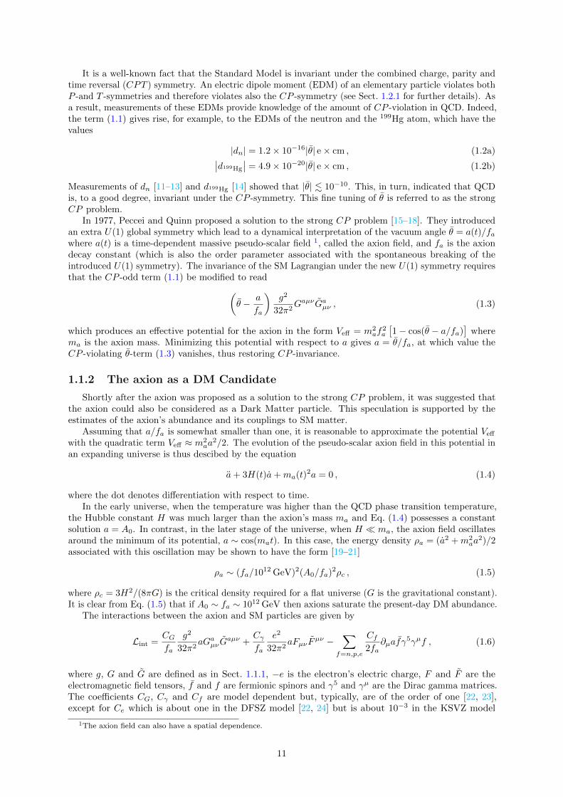
The Quantum Chromodynamics (QCD) Lagrangian contains a parity (P )- and charge-parity(CP )-violating term

θg2

32π2GaµνGaµν , (1.1)

where θ is the QCD vacuum angle related to the amount of CP -violation, g2/4π is the strong couplingconstant, Gaµν and Gaµν = 1

2εµνρσGaρσ are the gluon field strengths and its dual and a = 1, 2, ..., 8 is the

color index. In principle, θ can take any value in the range −π ≤ θ ≤ π.

10

It is a well-known fact that the Standard Model is invariant under the combined charge, parity andtime reversal (CPT ) symmetry. An electric dipole moment (EDM) of an elementary particle violates bothP -and T -symmetries and therefore violates also the CP -symmetry (see Sect. 1.2.1 for further details). Asa result, measurements of these EDMs provide knowledge of the amount of CP -violation in QCD. Indeed,the term (1.1) gives rise, for example, to the EDMs of the neutron and the 199Hg atom, which have thevalues

|dn| = 1.2× 10−16|θ| e× cm , (1.2a)∣∣d199Hg

∣∣ = 4.9× 10−20|θ| e× cm , (1.2b)

Measurements of dn [11–13] and d199Hg [14] showed that |θ| . 10−10. This, in turn, indicated that QCDis, to a good degree, invariant under the CP -symmetry. This fine tuning of θ is referred to as the strongCP problem.

In 1977, Peccei and Quinn proposed a solution to the strong CP problem [15–18]. They introducedan extra U(1) global symmetry which lead to a dynamical interpretation of the vacuum angle θ = a(t)/fawhere a(t) is a time-dependent massive pseudo-scalar field 1, called the axion field, and fa is the axiondecay constant (which is also the order parameter associated with the spontaneous breaking of theintroduced U(1) symmetry). The invariance of the SM Lagrangian under the new U(1) symmetry requiresthat the CP -odd term (1.1) be modified to read(

θ − a

fa

)g2

32π2GaµνGaµν , (1.3)

which produces an effective potential for the axion in the form Veff = m2af

2a

[1− cos(θ − a/fa)

]where

ma is the axion mass. Minimizing this potential with respect to a gives a = θ/fa, at which value theCP -violating θ-term (1.3) vanishes, thus restoring CP -invariance.

1.1.2 The axion as a DM Candidate

Shortly after the axion was proposed as a solution to the strong CP problem, it was suggested thatthe axion could also be considered as a Dark Matter particle. This speculation is supported by theestimates of the axion’s abundance and its couplings to SM matter.

Assuming that a/fa is somewhat smaller than one, it is reasonable to approximate the potential Veff

with the quadratic term Veff ≈ m2aa

2/2. The evolution of the pseudo-scalar axion field in this potential inan expanding universe is thus descibed by the equation

a+ 3H(t)a+ma(t)2a = 0 , (1.4)

where the dot denotes differentiation with respect to time.In the early universe, when the temperature was higher than the QCD phase transition temperature,

the Hubble constant H was much larger than the axion’s mass ma and Eq. (1.4) possesses a constantsolution a = A0. In contrast, in the later stage of the universe, when H ma, the axion field oscillatesaround the minimum of its potential, a ∼ cos(mat). In this case, the energy density ρa = (a2 +m2

aa2)/2

associated with this oscillation may be shown to have the form [19–21]

ρa ∼ (fa/1012 GeV)2(A0/fa)2ρc , (1.5)

where ρc = 3H2/(8πG) is the critical density required for a flat universe (G is the gravitational constant).It is clear from Eq. (1.5) that if A0 ∼ fa ∼ 1012 GeV then axions saturate the present-day DM abundance.

The interactions between the axion and SM particles are given by

Lint =CGfa

g2

32π2aGaµνG

aµν +Cγfa

e2

32π2aFµν F

µν −∑

f=n,p,e

Cf2fa

∂µafγ5γµf , (1.6)

where g, G and G are defined as in Sect. 1.1.1, −e is the electron’s electric charge, F and F are theelectromagnetic field tensors, f and f are fermionic spinors and γ5 and γµ are the Dirac gamma matrices.The coefficients CG, Cγ and Cf are model dependent but, typically, are of the order of one [22, 23],except for Ce which is about one in the DFSZ model [22, 24] but is about 10−3 in the KSVZ model

1The axion field can also have a spatial dependence.

11

[25, 26]. In any case, if fa ∼ 1012 GeV so that axions saturate the DM content, the couplings betweenthese particles and the SM sector are very weak indeed. This is in agreement with the observationsmentioned in Sect. 1.1.

Recently, it was also pointed out that the axion may allow the formation of the so-called axion quarknuggets [27–31], which not only resolve the DM problem but also explain other puzzling cosmologicaland astrophysical observations such as the predominance of matter over antimatter in the universe[32, 33], the solar coronal heating puzzle [34], the primordial lithium problem [35, 36], the DAMA/LIBRAannual modulation [37, 38], the strange sky-quakes [39], the mysterious burst-like events observed by theTelescope Array Experiment [40, 41] and the x-ray seasonal variations observed by the XMM-Newtonobservatory [42]. These possibilities further improve the axion’s attractiveness and a ‘magical’ solution toa wide range of problems, thus making its empirical detection more and more imperative.

1.2 Elementary particles’ EDMs and the solution to the matter-antimatter asymmetry

Another standing puzzle for modern physics is the apparent asymmetry between matter and antimatter[43]. The Big Bang should have produced equal amounts of matter and antimatter, which would thenannihilate one another off completely. The existence of the material world implies, on the other hand, thata tiny portion of matter, about five parts in ten billion, survived. A solution to this apparent asymmetryis a major part of the question that has troubled the human race since the dawn of civilization: ‘Why arewe here?’.

In 1967, Sakharov proposed three conditions necessary for the predominance of matter over antimatter[32]. Among these conditions is the violation of the CP -symmetry. As discussed in Sect. 1.1.1, the sourcefor CP -violation in the QCD sector is small, too small, in fact, to completely account for the observedmatter-antimatter asymmetry. Experiments searching for CP -violation in the leptonic sector by using, forexample, neutrino oscillations [44–46], are ongoing. In this thesis, I investigate the possibility of searchingfor CP -violation in the hadronic sector, particularly, in terms of the nucleon EDMs and CP -odd nuclearforces.

1.2.1 CP -violation and elementary particles’ EDMs

A EDM of an elementary particle violates both parity (P ) and time reversal symmetry (T ). This maybe understood by considering, for example, a nucleon carrying a magnetic dipole moment µ and an EDMd. Under time reversal, µ changes its sign but d remains the same so time invariance is violated. Underparity, d changes its direction, but µ stays the same, so the parity symmetry is also violated. Due to thevirtue of the CPT theorem, T -violation imply CP -violation.

The EDM of a nucleon may arise from those of its constituent quarks, but it may also arise dueto the CP -odd interactions with pion [47, 48]. At the same time, the pion can also mediate CP -oddinternucleon interactions, as was noted in Ref. [49]. Altogether, the nucleon EDMs and the CP -oddinternucleon forces give rise to the EDM of the nucleus, which could, in principle, be detected by placingthe nucleus in a combination of magnetic and electric fields and measuring the energy difference betweentwo configurations where the fields are parallel and anti-parallel.

1.2.2 Schiff’s theorem and methods to circumvent it

In measuring nuclear EDMs, it is natural to work with atoms and molecules. However, it is knownthat the nucleus of a neutral atom or molecule is completely shielded from any constant electric field, aresult often called the Schiff’s theorem [50]. This theorem may be understood if one notes that a neutralatom or molecule does not accelerate in a constant electric field, so an atomic or molecular nucleus doesnot accelerate either, meaning no field on the nucleus. Physically, the external electric field deforms theatomic or molecular electronic cloud in such a way that the internal electric field it creates at the nucleusexactly cancels the external field.

The Schiff’s theorem forces conventional EDM experiments to measure, instead of nuclear EDMs, therelated Schiff moment which arises due to the nucleus’ finite size. The atomic or molecular EDM inducedby this nuclear Schiff moment is typically about a thousand time smaller than the nuclear EDM itself.As a result, it would be experimentally advantageous to be able to access the nuclear EDM directly. Inthis thesis, I present different methods through which this goal may be achieved.

12

For example, I demonstrated that oscillating electric fields are not hindered by Schiff’s theorem. Thephysical picture for this result is clear: since the electronic cloud has inertia, it does not react instantlyto an oscillating electric field; it is this delayed response which allows for the penetration of the externalfield. This fact is even more pronounced in molecules where nuclei, which also participate in screening,have even larger inertia. These results are presented in Chapter 4.

Nuclear EDMs may also be oscillating if they are induced by axion Dark Matter [48]. I studied theeffects of these oscillating nuclear EDMs on atoms and molecules. Physically, such an oscillating nuclearEDM acts as a time-dependent perturbation to the electron cloud (and other nuclei in a molecule), thusreduces its screening ability, thus inducing a non-zero atomic or molecular EDM. If one then applies anoscillating electric field, observable nuclear spin precession happens. These possibilities are presented inChapter 5.

Chapter 6 is devoted to the study of the atomic and molecular transitions that may be induced byoscillating nuclear EDMs, Schiff moments and magnetic quadrupole moments.

Chapters 7 and 8 present another possibility to overcome Schiff’s theorem, namely, by taking intoaccount the magnetic interaction between electrons and nucleons. It will be demonstrated that a combinedelectric and magnetic interaction indeed gives rise to measurable atomic and molecular EDMs. Comparingthe contribution of this interaction with that of the phenomenological electron-nucleon contact interactionallows ones to place independent constraints on various CP -violating hadronic parameters.

Finally, chapter 9 presents an attempt to improve the accuracy of existing computations of the Schiffmoment’s interaction with electrons. The result of this chapter is important for deriving bounds on theSchiff moment from results of experiments with molecules.

Bibliography

[1] F. Zwicky, Helv. Phys. Acta 6, 110 (1933).

[2] F. Zwicky, Astrophys. J. 86, 217 (1937).

[3] V. C. Rubin and W. K. Ford Jr, Astrophys. J. 159, 379 (1970).

[4] V. C. Rubin, W. K. Ford Jr, and N. Thonnard, Astrophys. J. 238, 471 (1980).

[5] M. Markevitch, A. H. Gonzalez, D. Clowe, A. Vikhlinin, W. Forman, C. Jones, S. Murray, andW. Tucker, Astrophys. J 606, 819 (2004).

[6] D. Clowe, A. Gonzalez, and M. Markevitch, Astrophys. J. 604, 596 (2004).

[7] D. Clowe, M. Bradac, A. H. Gonzalez, M. Markevitch, S. W. Randall, C. Jones, and D. Zaritsky,Astrophys. J. 648, L109 (2006).

[8] G. Hinshaw, J. L. Weiland, R. S. Hill, N. Odegard, D. Larson, C. L. Bennett, J. Dunkley, B. Gold,M. R. Greason, N. Jarosik, et al., Astrophys. J., Suppl. Ser. 180, 225 (2009).

[9] G. Bertone, D. Hooper, and J. Silk, Phys. Rep. 405, 279 (2005).

[10] K. Olive, Chin. Phys. C 40, 100001 (2016).

[11] C. A. Baker, D. D. Doyle, P. Geltenbort, K. Green, M. G. D. van der Grinten, P. G. Harris, P. Iaydjiev,S. N. Ivanov, D. J. R. May, J. M. Pendlebury, et al., Phys. Rev. Lett. 97, 131801 (2006).

[12] J. M. Pendlebury et al., Phys. Rev. D 92, 092003 (2015).

[13] C. Abel, S. Afach, N. J. Ayres, C. A. Baker, G. Ban, G. Bison, K. Bodek, V. Bondar, M. Burghoff,E. Chanel, et al., Phys. Rev. Lett. 124, 081803 (2020).

[14] B. Graner, Y. Chen, E. G. Lindahl, and B. R. Heckel, Phys. Rev. Lett. 116, 161601 (2016).

[15] R. D. Peccei and H. R. Quinn, Phys. Rev. Lett. 38, 1440 (1977).

[16] R. D. Peccei, The Strong CP Problem and Axions (Springer, Berlin, Heidelberg, 2008), pp. 3–17.

[17] S. Weinberg, Phys. Rev. Lett. 40, 223 (1978).

[18] F. Wilczek, Phys. Rev. Lett. 40, 279 (1978).

13

[19] J. Preskill, M. B. Wise, and F. Wilczek, Phys. Lett. B 120, 127 (1983).

[20] L. Abbott and P. Sikivie, Phys. Lett. B 120, 133 (1983).

[21] M. Dine and W. Fischler, Physics Letters B 120, 137 (1983).

[22] J. E. Kim, Phys. Rev. Lett. 43, 103 (1979).

[23] M. Srednicki, Nucl. Phys. B 260, 689 (1985).

[24] M. Shifman, A. Vainshtein, and V. Zakharov, Nucl. Phys. B 166, 493 (1980).

[25] M. Dine, W. Fischler, and M. Srednicki, Phys. Lett. B 104, 199 (1981).

[26] A. Zhitnitsky, Sov. J. Nucl. Phys. 31, 260 (1980).

[27] D. Budker, V. V. Flambaum, X. Liang, and A. Zhitnitsky, Phys. Rev. D 101, 043012 (2020).

[28] A. Zhitnitsky, arXiv:2008.04325 (2020).

[29] D. Budker, V. V. Flambaum, and A. Zhitnitsky, arXiv:2003.07363 (2020).

[30] S. Ge, M. S. R. Siddiqui, L. V. Waerbeke, and A. Zhitnitsky, arXiv:2009.00004 (2020).

[31] S. Ge, H. Rachmat, M. S. R. Siddiqui, L. V. Waerbeke, and A. Zhitnitsky, arXiv:2004.00632 (2020).

[32] A. Sakharov, JTEP Lett. 5, 24 (1967).

[33] A. D. Sakharov, Sov. Phys. Usp. 34, 392 (1991).

[34] W. Grotrian, NW 27, 214 (1939).

[35] R. H. Cyburt, B. D. Fields, and K. A. Olive, J. Cosmo. Astropart. Phys. 2008, 012 (2008).

[36] R. H. Cyburt, B. D. Fields, K. A. Olive, and T.-H. Yeh, Rev. Mod. Phys. 88, 015004 (2016).

[37] R. Bernabei et al., Eur. Phys. J. C 67, 39 (2010).

[38] R. Bernabei, P. Belli, F. Cappella, V. Caracciolo, S. Castellano, R. Cerulli, C. Dai, A. d’Angelo,S. d’Angelo, A. Di Marco, et al., Eur. Phys. J. C 73, 2648 (2013).

[39] The Elginfield Infrasound Array (ELFO): Interesting (non-meteoric) events detected by ELFO,aquarid.physics.uwo.ca/research/infrasound/is_mysteriousexplosions.html, August 1,2008.

[40] R. Abbasi et al., Phys. Lett. A 381, 2565 (2017).

[41] T. Okuda, J. Phys. Conf. Ser. 1181, 012067 (2019).

[42] G. Fraser, A. Read, S. Sembay, J. Carter, and E. Schyns, Mon. Not. R. Astron. Soc. 445, 2146(2014).

[43] L. Canetti, M. Drewes, and M. Shaposhnikov, New J. Phys. 14, 095012 (2012).

[44] K. Dick, M. Freund, M. Lindner, and A. Romanino, Nuclear Physics B 562, 29 (1999).

[45] H. Nunokawa, S. Parke, and J. W. Valle, Progress in Particle and Nuclear Physics 60, 338 (2008).

[46] K. Abe, R. Akutsu, A. Ali, C. Alt, C. Andreopoulos, L. Anthony, M. Antonova, S. Aoki, A. Ariga,Y. Asada, et al., Nature 580, 339 (2020).

[47] R. J. Crewther, P. Di Vecchia, G. Veneziano, and E. Witten, Phys. Let. B 88, 123 (1979).

[48] P. W. Graham and S. Rajendran, Phys. Rev. D 84, 055013 (2011).

[49] O. P. Sushkov, V. V. Flambaum, and I. B. Khriplovich, Zh. Eksp. Teor. Fiz 87, 1521 (1984).

[50] L. I. Schiff, Phys. Rev. 132, 2194 (1963).

14

Chapter 2

Interference-assisted resonantdetection of axions

2.1 Overview

In this chapter, I consider a proposal to detect axion DM. This new scheme exploits the resonance ofaxions and photons by atoms and molecules. By arranging for the absorption amplitudes to interfere,one may achieve an axion signal that is linear in the axion-electron coupling constant, making the newscheme more advantageous than conventional axion searches.

These results are published in the following papers:

1. V. V. Flambaum, I. B. Samsonov, H. B. Tran Tan, Y. V. Stadnik and D. Budker, Interference-assisted resonant detection of axions, Phys. Dark Universe 24, 100272 (2019), arXiv:1803.09388,

2. V. V. Flambaum, I. B. Samsonov, H. B. Tran Tan, Y. V. Stadnik and D. Budker, Resonantdetection and production of axions with atoms, Int. J. Mod. Phys. A 33, 31, 1844030(2018),

which I have presented them at one international conference, one national conference and one nationalcompetition:

1. Searching for Axions and Axionic Dark Matter with Interference and Axion-inducedNuclear Moments, TeV Particle Astrophysics Conference, University of Sydney, Sydney, Australia,December 2019,

2. Effects of Dark Matter in atomic and molecular phenomena, Australian Institute of PhysicsPostgraduate Presentation Competition, University of Technology Sydney, Sydney, Australia,October 2019,

3. Detection of Axions Using Atomic Transitions Induced by Interference between Elec-tromagnetic and Axion Fields, Australian Institute of Physics Summer Meeting, University ofNew South Wales, Sydney, Australia, December 2017.

2.2 Abstract

Detection schemes for the quantum-chromodynamics axions and other axion-like particles in light-shining-through-a-wall (LSW) experiments are based on the conversion of these particles into photons ina magnetic field. An alternative scheme may involve the detection via a resonant atomic or moleculartransition induced by resonant axion absorption. The signal obtained in this process is second orderin the axion-electron interaction constant but may become first order if we allow interference betweenthe axion-induced transition amplitude and the transition amplitude induced by the electromagneticradiation that produces the axions.

15

2.3 Introduction

The axion is a light pseudoscalar particle proposed by Peccei and Quinn in 1977 to resolve thestrong CP (charge and parity) problem in quantum chromodynamics (QCD) [1–4]. Since then, theaxion and other feebly interacting pseudoscalar particles with similar properties (axion-like particles orALPs) have been identified as possible candidates to explain the observed Dark Matter (DM). Despitenumerous theoretical speculations, there is still no definitive experimental evidence for the existence ofthese particles. The reason for this lack of evidence is two-fold. The first difficulty arises from the factthat the coupling constants of the interactions of axions 1 with Standard-Model (SM) particles, althoughnot known precisely, are constrained to be small. As a result, any attempt to detect axions must seek toenhance the effects of the interactions and render them observable. This task is formidable. The seconddifficulty is that the axion’s mass is poorly constrained, so experiments that search for axions must covera large range of frequencies. In recent years, significant efforts, both theoretical and experimental, havebeen made to investigate the possible parameter spaces in mass and coupling strengths.

Traditional searches for axions are based mainly on the interaction between axions and photons in thepresence of a magnetic field. In such a situation, the mixing of the axion and photon states is possibleand the two types of particles can interconvert with one another [5, 6]. Helioscope experiments includingSumico [7–11], CAST [12–15], SOLAX [16, 17], COSME [18], DAMA [19–21], CDMS [22–25] and IAXO[26–28] convert solar axions into photons for detection. Haloscope experiments such as ADMX [29–31],HAYSTAC [32, 33] and ORGAN [34] convert cosmic axions into photons in microwave cavities anddetect these photons resonantly with SQUIDs. A notable feature of haloscope experiments is the longscanning time: since the energy of the incoming axions is not known, these experiments have to sweep alarge frequency range to find a resonance. Light-shining-through-a-wall (LSW) experiments includingALPS [35–37], OSQAR [38–40] and GammeV [41] involve converting photons into axions, passing theresulting beam through a wall, which blocks all the photons but not the axions, and then converting thetransmitted axions back into photons for detection on the other side of the wall. These LSW experimentsdo not involve frequency scanning since the energy of the axion is known from energy conservation.However, since the axion signals in these experiments scale to the fourth power in the axion-photoncoupling constant (instead of to the second power as in helio- and haloscope experiments), the sensitivityis greatly compromised. Finally, experiments like PVLAS [42–44], Q & A [45] and BMV [46, 47] searchfor optical birefringence (difference in optical refractive indices for different polarizations) and dichroism(difference in absorption of light of different polarizations) due to interconversion with axions [48].

Recently, various new schemes for axion detection have been proposed. These include searching foraxions by converting them into magnons in a ferromagnet [49, 50], by looking for parity- and time-reversal-invariance-violating effects (due to couplings of axions to SM particles) such as oscillating electric dipolemoments [51–55], by using dielectric haloscopes (improved sensitivity compared to traditional haloscopes)[56–59], by using nuclear magnetic resonance to search for axion-mediated CP-violating forces [60–63], byresonantly detecting the oscillating magnetic flux sourced by the axions entering a static magnetic field[64], by using electron spin resonance in magnetized media to detect the oscillating effective magneticfield induced by axions [65], by using superconductors [66] and semiconductors [67], by using an LCcircuit (Dark Matter radio) [68–70], by using Josephson junctions [71, 72], by using photon interferometry[73], by using axion-induced resonant molecular transitions [74], by using laser-spectroscopy techniques toprobe axion-induced atomic and molecular tranistions [75], by looking for an axion-induced topologicalCasimir effect [76] and by using a photon field (instead of a magnetic field) to trigger axion-to-photondecay then detecting the product photons with Raman scattering [77]. In this paper, we explore somepossible experimental schemes which are based on atomic or molecular transitions due to the absorptionof axions.

The idea of using atomic transitions to produce and detect axions dates back to a 1988 paper byZioutas and Semertzidis [78]. The authors proposed using an M1 transition to produce axions whichwould then be detected in a microwave cavity. In 2014, Sikivie extended this idea and proposed using theaxion-induced M1 transitions to detect galactic-halo axions [79]. In Sikivie’s scheme, atoms in the groundstate 0 absorb axions and go to an excited state i. A laser is then used to further excite the atoms to thestate f . This laser must be tuned so that it can only cause the i→ f transition. Photons emitted whenthe atoms in the state f decay are then detected. Following Sikivie’s paper, an experimental realizationthat uses Zeeman states in molecular oxygen at a temperature of 280 mK was proposed [80]. In thisparticular proposal, the transition frequency is scanned by applying a strong magnetic field and the

1In this paper, we will not distinguish between the QCD axion and other axion-like particles. The term ‘axion’ will referto both.

16

detection is done via resonant multiphoton-ionization (REMPI) spectroscopy.A general feature of the processes considered in the atom- or molecule-based proposals above is the

quadratic dependence of the detection rate on the axion-electron coupling constant. Since this constant issmall, the detection rate is minuscule. A possible enhancement of this rate may be achieved by allowingthe atoms to absorb a coherent mixture of axions and photons. The detection rate will then contain across term due to the interference between the axion- and photon-induced atomic transition amplitudes.This cross term is linear in the axion-electron coupling constant. In this paper, we explore this idea ofaxion-photon interference by propopsing and studing a scheme which resembles the traditional ALPSexperiment. We find that the sensitivity of our scheme may be better than that of existing helioscopeexperiments [14]. This fact is certainly interesting if one notes that the axions used in our scheme have tobe artificially produced and are thus not as abundant in number as the solar axions detected by helioscopeexperiments.

The rest of this paper will be organized as follows. In Sect. 2.4, we will give a general description ofthe experimental set-up and target choice for our scheme. In Sect. 2.5, all relevant formulae for transitionamplitudes, signal and signal-to-noise ratio for our scheme will be presented. Sect. 2.6 contains numericalestimates for some particular targets and a discussion of our scheme’s sensitivity to the product gaeegaγγ .In Sect. 2.7, we summarize our findings and provide some extra remarks. In Appendix A, for completeness,we discuss an alternative choice of target for our experiment which was not presented in the main text.Specifically, we consider in Appendix A the axion-induced M0 atomic transition and compare it with theM1 transitions presented in the main text. As it turns out, an M0-type experiment is not as competitiveas an M1-type one. In Appendix B, we study, as an offshoot of the axion-induced atomic transitioncalculation, the possibility of using atom transitions to make axion ’lasers’.

2.4 Experimental scheme

2.4.1 General set-up

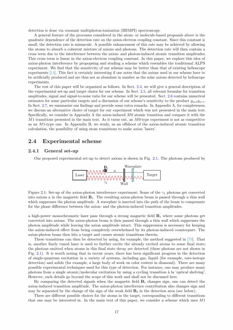
Our proposed experimental set-up to detect axions is shown in Fig. 2.1. The photons produced by

Figure 2.1: Set-up of the axion-photon interference experiment: Some of the γ1 photons get convertedinto axions a in the magnetic field B1. The resulting axion-photon beam is passed through a thin wallwhich suppresses the photon amplitude. A waveplate is inserted into the path of the beam to compensatefor the phase difference between the axion- and the photon-induced transition amplitudes.

a high-power monochromatic laser pass through a strong magnetic field B1 where some photons getconverted into axions. The axion-photon beam is then passed through a thin wall which suppresses thephoton amplitude while leaving the axion amplitude intact. This suppression is necessary for keepingthe axion-induced effect from being completely overwhelmed by its photon-induced counterpart. Theaxion-photon beam then hits a target and causes atomic transitions therein.

These transitions can then be detected by using, for example, the method suggested in [79]. Thatis, another finely tuned laser is used to further excite the already excited atoms to some final state;the photons emitted when atoms in this final state decay are detected (these photons are not shown inFig. 2.1). It is worth noting that in recent years, there has been significant progress in the detectionof single-quantum excitation in a variety of systems, including gas, liquid (for example, rare-isotopedetection) and solids (for example, a large body of work on color centers in diamond). There are manypossible experimental techniques used for this type of detection. For instance, one may produce manyphotons from a single atomic/molecular excitation by using a cycling transition a la ‘optical shelving’.However, such details go beyond the scope of this work and shall not be discussed here.

By comparing the detected signals when the magnetic field B1 changes sign, one can detect theaxion-induced transition amplitude. The axion-photon interference contribution also changes sign andmay be separated by the change of the sign of the weak field B2 in the detection area (see below).

There are different possible choices for the atoms in the target, corresponding to different transitionsthat one may be interested in. In the main text of this paper, we consider a scheme which uses M1

17

transitions, which appear to be the most advantageous choice. In the Appendix, a scheme with M0transition shall be considered. It appears that the M0 experiment is not as advantageous as its M1counterpart. Nevertheless, for completeness, we present both schemes in this paper.

2.4.2 Atomic transition

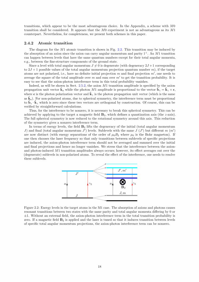
The diagram for the M1 atomic transition is shown in Fig. 2.2. This transition may be induced bythe absorption of an axion since the axion can carry angular momentum and parity 1+. An M1 transitioncan happen between levels that have the same quantum numbers except for their total angular momenta,e.g., between the fine-structure components of the ground state.

Since a level with total angular momentum J 6= 0 is degenerate (with degeneracy 2J + 1 correspondingto 2J + 1 possible values of the total angular momentum projection quantum number m), if the targetatoms are not polarized, i.e., have no definite initial projection m and final projection m′, one needs toaverage the square of the total amplitude over m and sum over m′ to get the transition probability. It iseasy to see that the axion-photon interference term in this total probability vanishes.

Indeed, as will be shown in Sect. 2.5.2, the axion M1 transition amplitude is specified by the axionpropagation unit vector ka while the photon M1 amplitude is proportional to the vector bγ = kγ × ε,

where ε is the photon polarization vector and kγ is the photon propagation unit vector (which is the same

as ka). For non-polarized atoms, due to spherical symmetry, the interference term must be proportionalto bγ · kγ which is zero since these two vectors are orthogonal by construction. Of course, this can beverified by straightforward calculations.

Thus, for the interference to be nonzero, it is necessary to break this spherical symmetry. This can beachieved by applying to the target a magnetic field B2, which defines a quantization axis (the z-axis).The full spherical symmetry is now reduced to the rotational symmetry around this axis. This reductionof the symmetry gives a nonzero interference term.

In terms of energy levels, the field B2 lifts the degeneracy of the initial (total angular momentumJ) and final (total angular momentum J ′) levels. Sublevels with the same J (J ′) but different m (m′)are now distinct (with energy separations of the order of µ0B2 where µ0 is the Bohr magneton). Ifone then chooses the laser frequency so that only transitions between sublevels of specific projectionsare induced, the axion-photon interference term should not be averaged and summed over the initialand final projections and hence no longer vanishes. We stress that the interference between the axion-and photon-induced M1 transition amplitudes always occurs; however, its effect averages out over the(degenerate) sublevels in non-polarized atoms. To reveal the effect of the interference, one needs to resolvethese sublevels.

Figure 2.2: Energy levels in the target atoms in the M1 case. The absorption of axions and photons causesresonant transitions between two states with the same parity and total angular momenta differing by 0 or±1. Without an external field, the axion-photon interference term in the total transition probability iszero. If a magnetic field B2 is applied and the laser is tuned so that it induces transition between levelsof specific total angular momentum projections, the axion-photon interference term can be nonzero.

18

2.5 Calculations

2.5.1 Photon-to-axion conversion probability

The interaction between axions and photons is described by the Lagrangian density

Laγγ = −gaγγ4

aFµν Fµν , (2.1)

where gaγγ is the axion-photon coupling constant, a is the axion field, Fµν and Fµν are the electromagneticfield tensor and its dual. This interaction is responsible for the interconversion between photons andaxions in a magnetic field B1, with the conversion probability given in the natural units (~ = c = 1) by[81, 82]

P =ω

4ka(gaγγB1l0)

2F 2 (q) , (2.2)

where ω is the photon energy (equal to the axion energy), ka is the axion’s momentum, l0 is the spatialextent of the magnetic field in the direction of the axion-photon beam direction, q = ω − ka is themomentum transferred from the photon field to the axion field and F (q) =

∫e−iqx (B (x) /B1l) dx is a

form factor. For a homogeneous magnetic field B1, formula (2.2) simplifies to

P =(gaγγB1l0)

2

4sinc2

(M2l0

4ω

). (2.3)

where M2 = m2a + 2ω2 (n− 1), ma is the axion mass, n is the photon refractive index and sinc (x) =

sin (x) /x. We will not need these formulae explicitly in the calculations below. The only quantity weneed for a numerical estimate is P.

According to the projected sensitivity of the ALPS II experiment [83], which features l0 = 100 m andB1 = 5.3 T, the upper limit on the axion-photon coupling constant gaγγ (2× 10−11 GeV−1) correspondsto the photon-to-axion conversion probability P ∼ 10−7. We will use these values in our estimates below.

Note that although not shown here, it is clear that the amplitude for the photon-to-axion conversionprocess is linear in B1 (this must be true since the conversion probability is quadratic in B1) and thisamplitude will change its sign when B1 does. We will exploit this observation to detect axions, asexplained in the sections below.

2.5.2 Atomic transition amplitudes

Photon absorption amplitude

The amplitude for an atomic transition A → B induced by the absorption of a photon is given by[84–86]

Mγ = i√

2πnγωγe−iωγtMγ

BA , (2.4)

where ωγ is the photon energy, nγ is the photon number density in the beam and MγBA is the transition

matrix element. The photon energy ωγ needs to match the difference of the energy levels Ei − E1S0,

corresponding to the resonant transition.The M1 photon matrix element Mγ

BA is given by

MγBA =

e

2mebγ · 〈B|J + S |A〉 , (2.5)

where bγ = kγ × ε is the direction of the magnetic component of the photon field (kγ is the photonpropagation unit vector and ε is the photon polarization vector), J is the electron’s total angularmomentum and S is the electron’s spin.

If we now fix a spherical basis e−1, e0, e1 with the quantization axis e0 in the direction of theapplied field B2, we can write the components of the vector bγ as bqγ where q = −1, 0, 1. We can alsodescribe the states A and B by the quantum numbers n, j, l,m and n′, j′, l′,m′, respectively. The M1photon matrix element thus reads

MγBA = (−1)

j′−m′bqγ

(j′ 1 j−m′ q m

)J , (2.6)

where

(j′ 1 j−m′ q m

)is the 3j symbol and J = e

2me〈n′j′l′‖J + S‖njl〉 is the reduced M1 matrix

element. Note that here and below, summations over the repeated indices p, q, ... are implicit.

19

Axion absorption amplitude

The interaction between the axion field a and the electron field ψ is described by the Lagrangiandensity

Lint = − gaee2me

∂µaψγ5γµψ , (2.7)

where gaee is the axion-electron coupling constant. This coupling constant can be written as

gaee =Ceme

fa, (2.8)

where fa is the axion decay constant and Ce is a model-dependent parameter. Currently, there are twomain models for the QCD axion: the KSVZ model [87, 88] and the DFSZ model [89, 90]. At tree-level,Ce = 0 for the KSVZ axion and Ce ∼ 1 for the DFSZ axion [91] (a nonzero value Ce ∼ α/2π ∼ 10−3

appears in the former case due to radiative corrections). Generic ALPs can have any Ce value.The amplitude for the atomic transition A → B induced by the absorption of an axion can be

calculated using a method similar to that used in the case of photon absorption. We find that

Ma = −√

2naωae−i(ωat+φa)Ma

BA , (2.9)

where ωa is the axion energy (which is equal to the energy of the γ1 photons, ωa = ωγ), φa is the axionphase (which differs from the photon phase by the phase of the field B1), na is the axion number densityin the beam and the matrix element Ma

BA can be derived from the interaction Lagrangian (2.7). In therelativistic limit (ωa ma), the leading-order terms of Ma

BA are [79, 92]

MaBA ≈ −

igaee2me

〈B| ka · S |A〉 −gaeeωa2me

〈B| r · S−(ka · S

)(ka · r

)|A〉 , (2.10)

where ka = ka/ωa is the axion propagation unit vector, r is the electron’s position vector and S = σ/2 isthe electron’s spin. The form of the matrix element can be qualitatively understood if we note that therelevant quantities in the problem are the electron’s momentum p (which can be replaced by r by usingthe identity p = ime [H0, r] where H0 in the unperturbed nonrelativistic electronic Hamiltonian), theelectron’s spin S and the axion’s momentum ka. The interaction Lagrangian, being a pseudoscalar, musttherefore be built from the scalar products of these vectors.

It can be shown that the first term in Eq. (2.10) is of M1 type whereas the second term is of M0type. Here, we are concerned only with the first term of Eq. (2.10). The M0 case will be considered inappendix A.

The axion M1 matrix element is thus given by

MaBA =

igaee2me

〈B| ka · S |A〉 = (−1)j′−m′ igaee

ekqa

(j′ 1 j−m′ q m

)S , (2.11)

where S = e2me〈n′j′l′‖S‖njl〉. The second line of Eq. (2.11) is obtained by assuming the same spherical

basis as above.

2.5.3 Axion signal and signal-to-noise ratio

Suppose that the source laser (laser 1) produces photons continuously at a rate of N photons perunit time. Passing through the magnetic field, PN of them get converted into axions where P is thephoton-axion conversion probability given by formula (2.3). Since P 1, the number of remainingphotons after conversion is approximately N . Denoting by T the photon-transmission coefficient of thewall, the number of incident photons per unit time is T N . Thus, the photon number density in Eq. (2.4)is nγ ∝ T N and the axion number density na in Eq. (2.9) is na ∝ PN .

The total amplitude for the A → B transition is the sum of those given by Eqs. (2.4) and (2.9).Squaring this sum and discarding the term which is second order in the axion-electron coupling constant,we find the total transition probability

P ∝ |Mγ |2 + 2 Re(iMaMγ

)(2.12)

(the bar denotes complex conjugation). The factor i comes from the inserted phase-compensatingwaveplate.

20

Multiplying this probability by the probability of transition from B to C (recall that to detect theatomic transitions, we further excite the atoms in the state B to some state C then detect the photonsemitted when atoms in this state decay), one finds the detection probability. Multiplying the detectionprobability by the number of atoms in the target and the detection coefficient, which includes theprobability of decay from the state C and the sensitivity of the detector, one gets the number of observedexcited atoms, which we denote by S. We assume that these stages of detection, associated with countingthe atoms excited to state B, have close to 100% efficiency.

We observe that as the magnetic field B1 changes sign, the phase φa changes by π. This correspondsto the interference term 2 Re

(iMaMγ

)flipping sign. The same thing happens if B2 change its sign.

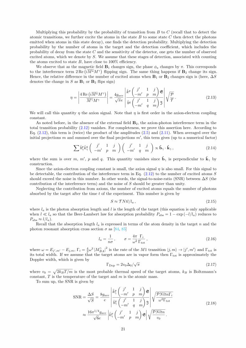
Hence, the relative difference in the number of excited atoms when B1 or B2 changes sign is (here, ∆Sdenotes the change in S as B1 or B2 flips sign)

η =

∣∣∣∣∣4 Re(iMaMγ

)MγMγ

∣∣∣∣∣ =4gaee√πe

∣∣∣∣∣∣∣∣kp(

j′ 1 j−m′ p m

)S

bq(

j′ 1 j−m′ q m

)J

∣∣∣∣∣∣∣∣√PT. (2.13)

We will call this quantity η the axion signal. Note that η is first order in the axion-electron couplingconstant.

As noted before, in the absence of the external field B2, the axion-photon interference term in thetotal transition probability (2.12) vanishes. For completeness, we prove this assertion here. According toEq. (2.12), this term is (twice) the product of the amplitudes (2.5) and (2.11). When averaged over theinitial projections m and summed over the final projections m′, this term gives (up to a numerical factor)∑

bpγ kqγ

(j′ 1 j−m′ p m

)(j′ 1 j−m′ q m

)∝ bγ · kγ , (2.14)

where the sum is over m, m′, p and q. This quantity vanishes since bγ is perpendicular to kγ byconstruction.

Since the axion-electron coupling constant is small, the axion signal η is also small. For this signal tobe detectable, the contribution of the interference term in Eq. (2.12) to the number of excited atoms Sshould exceed the noise in this number. In other words, the signal-to-noise-ratio (SNR) between ∆S (thecontribution of the interference term) and the noise of S should be greater than unity.

Neglecting the contribution from axions, the number of excited atoms equals the number of photonsabsorbed by the target after the time t of the experiment. This number is given by

S ≈ T Ntl/la , (2.15)

where la is the photon absorption length and l is the length of the target (this equation is only applicablewhen l la so that the Beer-Lambert law for absorption probability Pabs = 1− exp (−l/la) reduces toPabs ≈ l/la).

Recall that the absorption length la is expressed in terms of the atom density in the target n and thephoton resonant absorption cross section σ as [84, 85]

la =1

nσ, σ =

4π

ω2

ΓiΓtot

, (2.16)

where ω = Ej′,m′ − Ej,m, Γi = 43ω

3 |MγBA|

2is the rate of the M1 transition |j,m〉 → |j′,m′〉 and Γtot is

its total width. If we assume that the target atoms are in vapor form then Γtot is approximately theDoppler width, which is given by

ΓDop = 2v0∆0/√π (2.17)

where v0 =√

2kBT/m is the most probable thermal speed of the target atoms, kB is Boltzmann’sconstant, T is the temperature of the target and m is the atomic mass.

To sum up, the SNR is given by

SNR =∆S√S

=8gaeee

∣∣∣∣∣∣∣∣kpγ

(j′ 1 j−m′ p m

)S

bqγ

(j′ 1 j−m′ q m

)J

∣∣∣∣∣∣∣∣√PNltnΓiω2Γtot

≈ 16π1/4gaee√6e

∣∣∣∣kpγ ( j′ 1 j−m′ p m

)S

∣∣∣∣√PNltnv0

.

(2.18)

21

We observe that the SNR is independent of the wall’s transmission coefficient T but is proportional tothe square root of the total number of photons Nt and the target size l. Hence, to gain a better SNR, oneneeds a sufficiently powerful laser and a sufficiently large target to absorb as many photons as possible.

2.6 Numerical estimates

2.6.1 The M1 case - vapor target

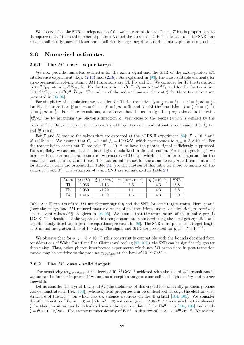
We now provide numerical estimates for the axion signal and the SNR of the axion-photon M1interference experiment, Eqs. (2.13) and (2.18). As explained in [93], the most suitable elements foran experiment involving atomic M1 transitions are Tl, Pb and Bi. We consider for Tl the transition6s26p 2P1/2 → 6s26p 2P3/2, for Pb the transition 6s26p2 3P0 → 6s26p2 3P1 and for Bi the transition6s26p3 4S3/2 → 6s26p3 2D3/2. The values of the reduced matrix element J for these transitions arepresented in [93–95].

For simplicity of calculation, we consider for Tl the transition |j = 12 ,m = 1

2 〉 → |j′ = 3

2 ,m′ = 1

2 〉,for Pb the transition |j = 0,m = 0〉 → |j′ = 1,m′ = 0〉 and for Bi the transition |j = 3

2 ,m = 32 〉 →

|j′ = 32 ,m

′ = 32 〉. For these transitions, we observe that the axion signal is proportional to the ratio∣∣∣k0

γ/b0γ

∣∣∣, so by arranging the photon’s direction kγ very close to the z-axis (which is defined by the

external field B2), one can make the axion signal large. For numerical estimates, we assume that k0γ ≈ 1

and b0γ ≈ 0.01.For P and N , we use the values that are expected at the ALPS II experiment [83]: P ∼ 10−7 and

N ≈ 1020 s−1. We assume that Ce ∼ 1 and fa = 109 GeV, which corresponds to gaee ≈ 5× 10−13. Forthe transmission coefficient T , we take T = 10−18 to have the photon signal sufficiently suppressed.For simplicity, we assume that the laser light is polarized in the z-direction. For the target length wetake l = 10 m. For numerical estimates, we choose t=100 days, which is the order of magnitude for themaximal practical integration times. The appropriate values for the atom density n and temperature Tfor different atoms are presented in Table 2.1 (see the caption of this table for more comments on thevalues of n and T ). The estimates of η and SNR are summarized in Table 2.1.

Atom ω (eV) J (e/2me) n(1017 cm−3

)η(×10−4

)SNR

Tl 0.966 -1.13 6.6 4.3 8.8Pb 0.969 -1.29 1.1 4.3 5.8Bi 1.416 -1.69 1.5 4.3 6.0

Table 2.1: Estimates of the M1 interference signal η and the SNR for some target atoms. Here, ω andJ are the energy and M1 reduced matrix element of the transitions under consideration, respectively.The relevant values of J are given in [93–95]. We assume that the temperature of the metal vapors is1473 K. The densities of the vapors at this temperature are estimated using the ideal gas equation andexperimentally fitted vapor pressure equations presented in [96]. The SNR corresponds to a target lengthof 10 m and integration time of 100 days. The signal and SNR are presented for gaee = 5× 10−13.

We observe that for gaee = 5× 10−13 (this constraint is compatible with the bounds obtained fromconsiderations of White Dwarf and Red Giant stars’ cooling [97–102]), the SNR can be significantly greaterthan unity. Thus, axion-photon interference experiments which use M1 transitions in post-transitionmetals may be sensitive to the product gaγγgaee at the level of 10−23 GeV−1.

2.6.2 The M1 case - solid target

The sensitivity to gaγγgaee at the level of 10−23 GeV−1 achieved with the use of M1 transitions invapors can be further improved if we use, as absorption targets, some solids of high density and narrowlinewidth.

Let us consider the crystal EuCl3 ·H2O (the usefulness of this crystal for coherently producing axionswas demonstrated in Ref. [103]), whose optical properties can be understood through the electron-shellstructure of the Eu3+ ion which has six valence electrons on the 4f orbital [104, 105]. We considerthe M1 transition |7F0,m = 0〉 → |5D1,m

′ = 0〉 with energy ω = 2.36 eV. The reduced matrix elementJ for this transition can be calculated using the spectral data of the Eu3+ ion [104, 105] and readsJ = S ≈ 0.17e/2me. The atomic number density of Eu3+ in this crystal is 2.7× 1021 cm−3. We assume

22

that the total width of this transition is Γtot ≈ 25 MHz (this width was realized in EuCl3 ·H2O for theE1 transition 7F0 → 5D0 [106]; for simplicity, we assume that the width of the M1 transition underconsideration is similar to this). Note that due to the high density and ultranarrow width, the M1 photonabsorption length in this crystal is very small, la ∼ 1 cm, so we must use, in Eq. (2.18), l ∼ la. As aresult, the SNR is

SNRsolid =4gaee√πe

∣∣∣∣∣ k0γ

b0γ

∣∣∣∣∣√PNtr , (2.19)

where r = l/la. Taking r ≈ 3, one obtains SNRsolid ≈ 20 for gaee = 5× 10−13. Thus, an experiment usingsolid targets with ultranarrow linewidths can reach the sensitivity gaγγgaee ∼ 10−24 GeV−1. This is anorder of magnitude better than the constraint obtained by multiplying the limits of ALPS-II and WhiteDwarf/Red Giant star cooling.

2.6.3 Comparison of projected sensitivities

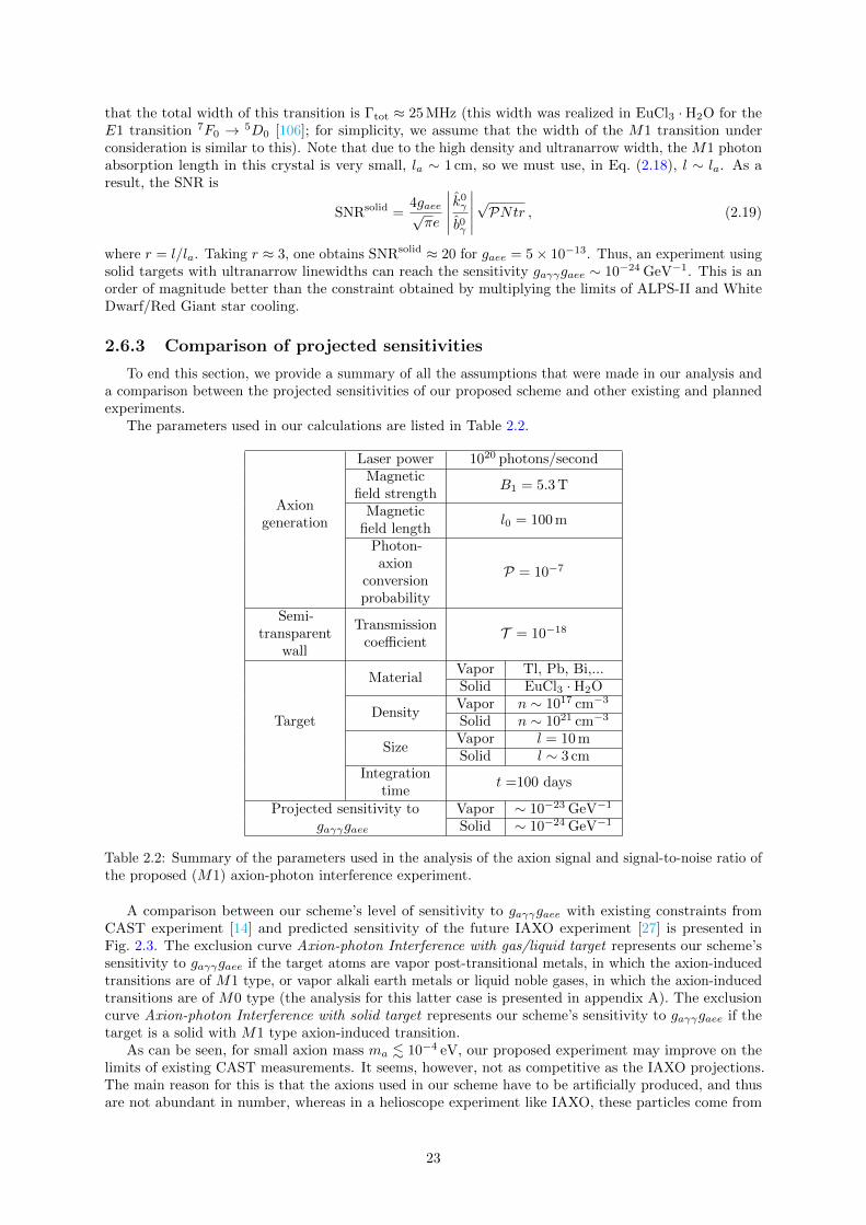
To end this section, we provide a summary of all the assumptions that were made in our analysis anda comparison between the projected sensitivities of our proposed scheme and other existing and plannedexperiments.

The parameters used in our calculations are listed in Table 2.2.

Axiongeneration

Laser power 1020 photons/secondMagnetic

field strengthB1 = 5.3 T

Magneticfield length

l0 = 100 m

Photon-axion

conversionprobability

P = 10−7

Semi-transparent

wall

Transmissioncoefficient

T = 10−18

Target

MaterialVapor Tl, Pb, Bi,...Solid EuCl3 ·H2O

DensityVapor n ∼ 1017 cm−3

Solid n ∼ 1021 cm−3

SizeVapor l = 10 mSolid l ∼ 3 cm

Integrationtime

t =100 days

Projected sensitivity togaγγgaee

Vapor ∼ 10−23 GeV−1

Solid ∼ 10−24 GeV−1

Table 2.2: Summary of the parameters used in the analysis of the axion signal and signal-to-noise ratio ofthe proposed (M1) axion-photon interference experiment.

A comparison between our scheme’s level of sensitivity to gaγγgaee with existing constraints fromCAST experiment [14] and predicted sensitivity of the future IAXO experiment [27] is presented inFig. 2.3. The exclusion curve Axion-photon Interference with gas/liquid target represents our scheme’ssensitivity to gaγγgaee if the target atoms are vapor post-transitional metals, in which the axion-inducedtransitions are of M1 type, or vapor alkali earth metals or liquid noble gases, in which the axion-inducedtransitions are of M0 type (the analysis for this latter case is presented in appendix A). The exclusioncurve Axion-photon Interference with solid target represents our scheme’s sensitivity to gaγγgaee if thetarget is a solid with M1 type axion-induced transition.

As can be seen, for small axion mass ma . 10−4 eV, our proposed experiment may improve on thelimits of existing CAST measurements. It seems, however, not as competitive as the IAXO projections.The main reason for this is that the axions used in our scheme have to be artificially produced, and thusare not abundant in number, whereas in a helioscope experiment like IAXO, these particles come from

23

the Sun in a large quantity. In that respect, it is actually surprising that our proposed scheme can reachand in some case surpass CAST’s sensitivity.

Figure 2.3: Comparison between constraints on the product gaγγgaee as a function of the axion mass ma

from the CAST experiment (existing) [14], the IAXO experiment (projected) [27] and the sensitivity ofthe experimental scheme proposed in this paper (projected).

We note that it is possible, at least within some specific axion models, to relate the two couplingconstants gaγγ and gaee. The latter is given in Eq. (2.8). The former may be expressed as [14]

gaγγ ≈α

2πfa

(E

N− 1.92

), (2.20)

where α is the fine-structure constant and E/N is the ratio of the electromagnetic and color anomalies ofthe Peccei-Quinn symmetry.

If we assume that the axion is described by the KSVZ model [87, 88] then Ce ∼ α/2π and E/N = 0.As a result, we obtain, from Eqs. (2.8) and (2.20)

gaγγ ≈ −3.8× 103gaeeGeV−1 . (2.21)

If, on the other hand, we assume that the axion is described by the DFSZ model [89, 90] then Ce ∼ 1and E/N = 8/3 so in this model, we have

gaγγ ≈ 1.7gaeeGeV−1 . (2.22)

The relations (2.21) and (2.22) allow us to convert our scheme’s sensitivity to |gaγγgaee| into asensitivity to gaγγ alone. This may then be compared to the projected limit on gaγγ by ALPS-II [83] aspresented in Fig. 2.4.

Figure 2.4: Comparison between the projected constraints on the coupling constant gaγγ as a functionof the axion mass ma from the ALPS-II experiment [83] and the sensitivity of the experimental schemeusing M1 atomic transition in a crystal proposed in this paper.

We conclude that for the DFSZ axion, our proposed scheme may have a better sensitivity to gaγγthan ALPS-II. However, for the KFSZ axion, our sensitivity to gaγγ is not as good as that of ALPS-II.Of course, since none of the axion models have been verified or falsified, it is not certain how gaee andgaγγ are related.

24

2.7 Conclusions

In this work, we have proposed and considered a scheme for the resonant detection of laboratory-produced axions and other axion-like particles. In this scheme, the axions are generated from photons ina magnetic field, as in current LSW experiments, and are then detected by using atomic (or molecular)transitions. The fundamental difference between this scheme and traditional LSW experiments is thatinstead of completely blocking the photons, we allow a small fraction of them to be absorbed by thetarget atoms. With such an allowance, the interference between the axion- and photon-induced transitionamplitudes occurs and the experimental signal now scales linearly with the axion-electron couplingconstant. This is an improvement over existing atom-based proposals whose signals have a quadraticdependence on the axion-electron coupling constant.

We have provided theoretical calculations and numerical estimates for a number of target atoms. Wefound that post-transition metals, in which axions induce transitions of M1 type, are potential candidatesfor experimental applications. This scheme may be realized as simple add-ons to the existing and plannedALPS experiments, with the photon-blocking wall replaced by some semi-transparent material and theaxion-to-photon reconversion unit replaced by a vapor cell. Whereas ALPS and ALPS-II measure thequantity gaγγ only, our scheme, as an upgrade to these experiments, allows one to also measure theproduct gaγγgaee. This means that with some relatively simple modifications, ALPS experiments canmeasure both gaγγ and gaee.

Our proposed scheme has a potential sensitivity to the product of the axion-photon and axion-electroncoupling constants gaγγgaee at the level of 10−24–10−23 GeV−1. This level of sensitivity is at least oneorder of magnitude better than the existing limit of CAST. By using known relations between gaee andgaγγ , we have shown that our proposed experiment is more sensitive to the DFSZ axion than ALPS-II.

It might be possible to increase the sensitivity to gaγγgaee by using heterodyne interferometry, whoseusefulness to ALPS-type experiments was studied in [107]. The authors of [107] suggested to interfere thephoton signal in an ALPS-type experiment with a laser of slightly different frequency. This generatesa time-varying signal, called the beat note (at the difference frequency) which is separated from theconstant photon background and is detected. The authors of [107] hope to achieve a sensitivity of 10−6

photons per second. Following this idea, we can consider a scheme in which the axion-generating photonsare blocked off completely (a completely opaque wall is used instead of a semi-transparent one) and theaxion-induced transition amplitude is allowed to interfere with the amplitude of the transition caused byphotons of slightly different frequency. The beat note in the total number of transitions is detected. Thisscheme may have some advantages over those considered in this paper. A detailed study of it will be thesubject of our future work.

Acknowledgments

We thank Carlo Rizzo for asking the right questions that triggered this work and for his advice on themanuscript and Vladimir Dzuba, Max Zolotorev and Joerg Jaeckel for helpful discussions. This workwas supported in part by the Australian Research Council Grant No. DP150101405, the GutenbergFellowship, the Humboldt Research Fellowship, the DFG Koselleck Program and the Heising-Simons andSimons Foundation. This project has also received funding from the European Research Council (ERC)under the European Union’s Horizon 2020 Research and Innovative Programme (grant agreement No.695405).

2.A Axion-photon interference with atomic transitions of M0type

2.A.1 Scheme description

As discussed in Sect. 2.5.2, axions can also induce atomic transition of M0 type (total angularmomentum is unchanged, parity is changed). In this appendix, we analyze the possibility of using M0transitions to detect axions.

An M0 transition might be realized if the atoms are chosen to have two valence electrons, with theground state 0 being ns2 1S0 and the first excited state being nsnp 3P0 (such atoms include Mg, Ca,Sr, Ba and Hg). In such atoms, the single-photon transition from the ground state 1S0 to the excitedstate 3P0 is forbidden. On the other hand, since an axion can carry the quantum numbers (angular

25

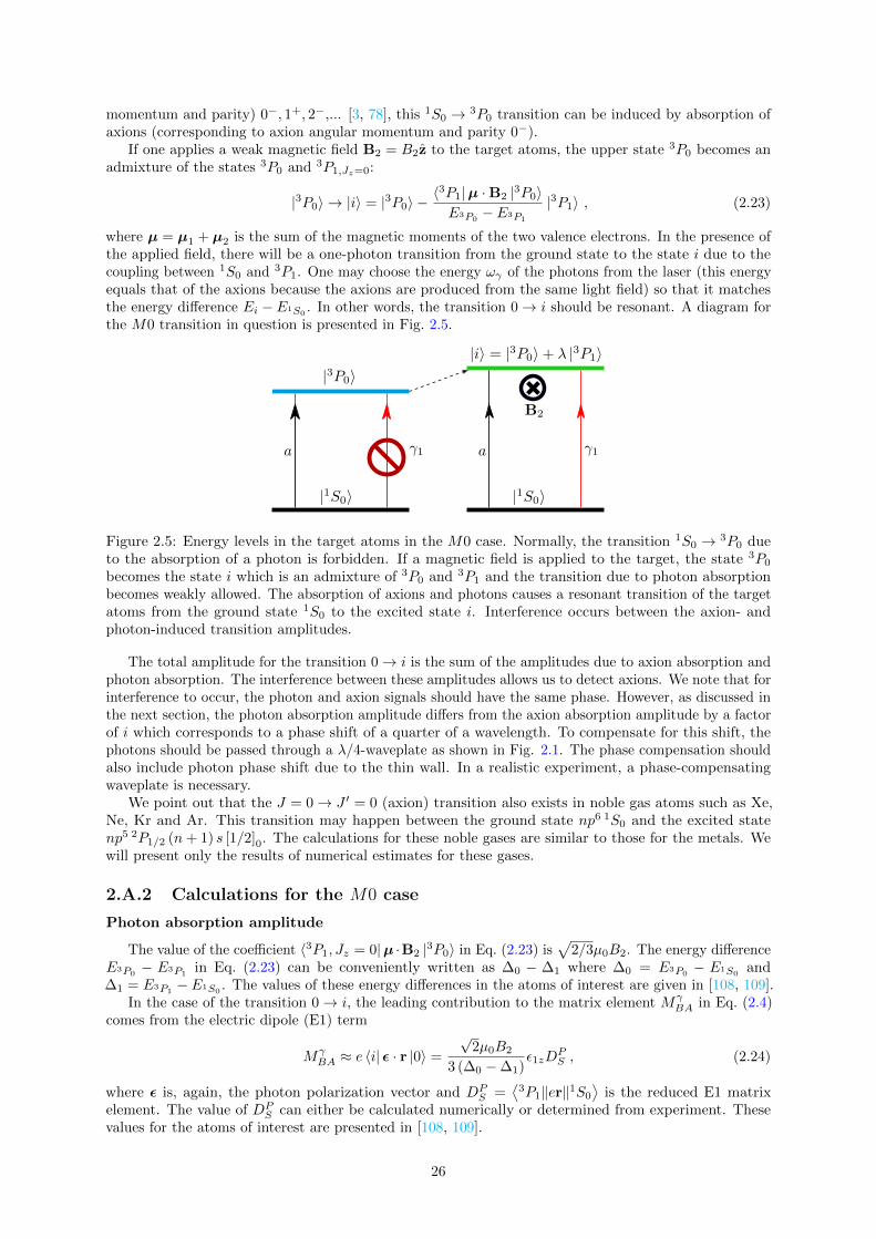
momentum and parity) 0−, 1+, 2−,... [3, 78], this 1S0 → 3P0 transition can be induced by absorption ofaxions (corresponding to axion angular momentum and parity 0−).

If one applies a weak magnetic field B2 = B2z to the target atoms, the upper state 3P0 becomes anadmixture of the states 3P0 and 3P1,Jz=0:

|3P0〉 → |i〉 = |3P0〉 −〈3P1|µ ·B2 |3P0〉E3P0

− E3P1

|3P1〉 , (2.23)

where µ = µ1 + µ2 is the sum of the magnetic moments of the two valence electrons. In the presence ofthe applied field, there will be a one-photon transition from the ground state to the state i due to thecoupling between 1S0 and 3P1. One may choose the energy ωγ of the photons from the laser (this energyequals that of the axions because the axions are produced from the same light field) so that it matchesthe energy difference Ei −E1S0

. In other words, the transition 0→ i should be resonant. A diagram forthe M0 transition in question is presented in Fig. 2.5.

Figure 2.5: Energy levels in the target atoms in the M0 case. Normally, the transition 1S0 → 3P0 dueto the absorption of a photon is forbidden. If a magnetic field is applied to the target, the state 3P0

becomes the state i which is an admixture of 3P0 and 3P1 and the transition due to photon absorptionbecomes weakly allowed. The absorption of axions and photons causes a resonant transition of the targetatoms from the ground state 1S0 to the excited state i. Interference occurs between the axion- andphoton-induced transition amplitudes.

The total amplitude for the transition 0→ i is the sum of the amplitudes due to axion absorption andphoton absorption. The interference between these amplitudes allows us to detect axions. We note that forinterference to occur, the photon and axion signals should have the same phase. However, as discussed inthe next section, the photon absorption amplitude differs from the axion absorption amplitude by a factorof i which corresponds to a phase shift of a quarter of a wavelength. To compensate for this shift, thephotons should be passed through a λ/4-waveplate as shown in Fig. 2.1. The phase compensation shouldalso include photon phase shift due to the thin wall. In a realistic experiment, a phase-compensatingwaveplate is necessary.

We point out that the J = 0→ J ′ = 0 (axion) transition also exists in noble gas atoms such as Xe,Ne, Kr and Ar. This transition may happen between the ground state np6 1S0 and the excited statenp5 2P1/2 (n+ 1) s [1/2]0. The calculations for these noble gases are similar to those for the metals. Wewill present only the results of numerical estimates for these gases.

2.A.2 Calculations for the M0 case

Photon absorption amplitude

The value of the coefficient 〈3P1, Jz = 0|µ ·B2 |3P0〉 in Eq. (2.23) is√

2/3µ0B2. The energy differenceE3P0

− E3P1in Eq. (2.23) can be conveniently written as ∆0 − ∆1 where ∆0 = E3P0

− E1S0and

∆1 = E3P1−E1S0

. The values of these energy differences in the atoms of interest are given in [108, 109].In the case of the transition 0→ i, the leading contribution to the matrix element Mγ

BA in Eq. (2.4)comes from the electric dipole (E1) term

MγBA ≈ e 〈i| ε · r |0〉 =

√2µ0B2

3 (∆0 −∆1)ε1zD

PS , (2.24)

where ε is, again, the photon polarization vector and DPS =

⟨3P1‖er‖1S0

⟩is the reduced E1 matrix

element. The value of DPS can either be calculated numerically or determined from experiment. These

values for the atoms of interest are presented in [108, 109].

26

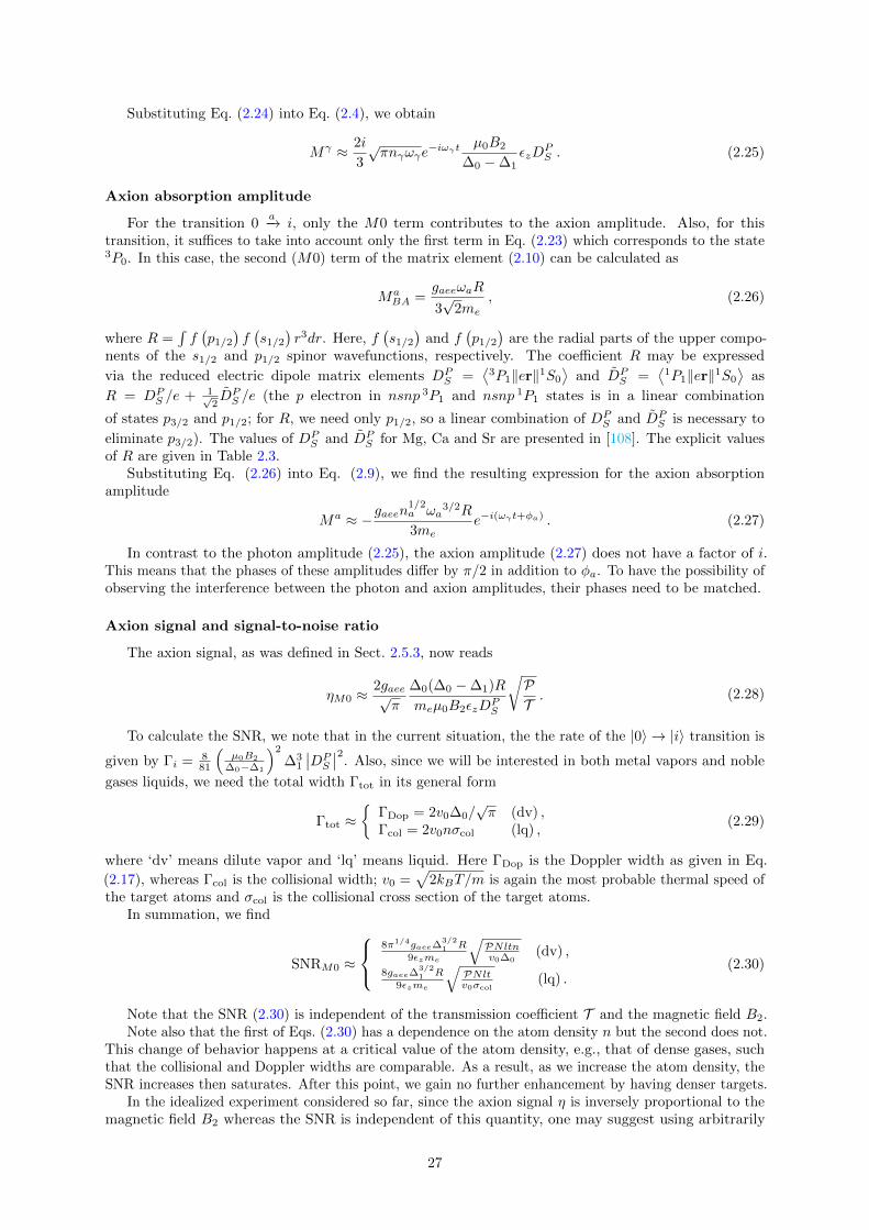
Substituting Eq. (2.24) into Eq. (2.4), we obtain

Mγ ≈ 2i

3

√πnγωγe

−iωγt µ0B2

∆0 −∆1εzD

PS . (2.25)

Axion absorption amplitude

For the transition 0a−→ i, only the M0 term contributes to the axion amplitude. Also, for this

transition, it suffices to take into account only the first term in Eq. (2.23) which corresponds to the state3P0. In this case, the second (M0) term of the matrix element (2.10) can be calculated as

MaBA =

gaeeωaR

3√

2me

, (2.26)

where R =∫f(p1/2

)f(s1/2

)r3dr. Here, f

(s1/2

)and f

(p1/2

)are the radial parts of the upper compo-

nents of the s1/2 and p1/2 spinor wavefunctions, respectively. The coefficient R may be expressed

via the reduced electric dipole matrix elements DPS =

⟨3P1‖er‖1S0

⟩and DP

S =⟨

1P1‖er‖1S0

⟩as

R = DPS /e + 1√

2DPS /e (the p electron in nsnp 3P1 and nsnp 1P1 states is in a linear combination

of states p3/2 and p1/2; for R, we need only p1/2, so a linear combination of DPS and DP

S is necessary to

eliminate p3/2). The values of DPS and DP

S for Mg, Ca and Sr are presented in [108]. The explicit valuesof R are given in Table 2.3.

Substituting Eq. (2.26) into Eq. (2.9), we find the resulting expression for the axion absorptionamplitude

Ma ≈ −gaeen1/2a ωa

3/2R

3mee−i(ωγt+φa) . (2.27)

In contrast to the photon amplitude (2.25), the axion amplitude (2.27) does not have a factor of i.This means that the phases of these amplitudes differ by π/2 in addition to φa. To have the possibility ofobserving the interference between the photon and axion amplitudes, their phases need to be matched.

Axion signal and signal-to-noise ratio

The axion signal, as was defined in Sect. 2.5.3, now reads

ηM0 ≈2gaee√π

∆0(∆0 −∆1)R

meµ0B2εzDPS

√PT. (2.28)

To calculate the SNR, we note that in the current situation, the the rate of the |0〉 → |i〉 transition is

given by Γi = 881

(µ0B2

∆0−∆1

)2

∆31

∣∣DPS

∣∣2. Also, since we will be interested in both metal vapors and noble

gases liquids, we need the total width Γtot in its general form

Γtot ≈

ΓDop = 2v0∆0/√π (dv) ,

Γcol = 2v0nσcol (lq) ,(2.29)

where ‘dv’ means dilute vapor and ‘lq’ means liquid. Here ΓDop is the Doppler width as given in Eq.

(2.17), whereas Γcol is the collisional width; v0 =√

2kBT/m is again the most probable thermal speed ofthe target atoms and σcol is the collisional cross section of the target atoms.

In summation, we find

SNRM0 ≈

8π1/4gaee∆

3/21 R

9εzme

√PNltnv0∆0

(dv) ,

8gaee∆3/21 R

9εzme

√PNltv0σcol

(lq) .(2.30)

Note that the SNR (2.30) is independent of the transmission coefficient T and the magnetic field B2.Note also that the first of Eqs. (2.30) has a dependence on the atom density n but the second does not.

This change of behavior happens at a critical value of the atom density, e.g., that of dense gases, suchthat the collisional and Doppler widths are comparable. As a result, as we increase the atom density, theSNR increases then saturates. After this point, we gain no further enhancement by having denser targets.

In the idealized experiment considered so far, since the axion signal η is inversely proportional to themagnetic field B2 whereas the SNR is independent of this quantity, one may suggest using arbitrarily

27

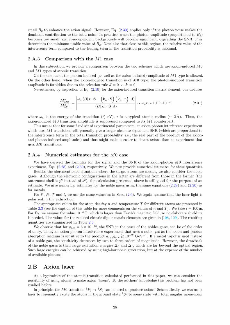
small B2 to enhance the axion signal. However, Eq. (2.30) applies only if the photon noise makes thedominant contribution to the total noise. In practice, when the photon amplitude (proportional to B2)becomes too small, signal-independent backgrounds will become significant, degrading the SNR. Thisdetermines the minimum usable value of B2. Note also that close to this regime, the relative value of theinterference term compared to the leading term in the transition probability is maximal.

2.A.3 Comparison with the M1 case

In this subsection, we provide a comparison between the two schemes which use axion-induced M0and M1 types of atomic transition.

On the one hand, the photon-induced (as well as the axion-induced) amplitude of M1 type is allowed.On the other hand, when the axion-induced transition is of M0 type, the photon-induced transitionamplitude is forbidden due to the selection rule J = 0 9 J ′ = 0.

Nevertheless, by inspection of Eq. (2.10) for the axion-induced transition matrix element, one deduces

∣∣∣∣MaM0

MaM1

∣∣∣∣ =

∣∣∣∣∣∣ωa 〈B| r · S−

(ka · S

)(ka · r

)|A〉

〈B| ka · S |A〉

∣∣∣∣∣∣ ∼ ωar ∼ 10−4–10−3 , (2.31)

where ωa is the energy of the transition (. eV), r is a typical atomic radius (∼ 2 A). Thus, theaxion-induced M0 transition amplitude is suppressed compared to its M1 counterpart.

This means that for some fixed set of experimental parameters, an axion-photon interference experimentwhich uses M1 transitions will generally give a larger absolute signal and SNR (which are proportional tothe interference term in the total transition probability, i.e., the real part of the product of the axion-and photon-induced amplitudes) and thus might make it easier to detect axions than an experiment thatuses M0 transitions.

2.A.4 Numerical estimates for the M0 case

We have derived the formulae for the signal and the SNR of the axion-photon M0 interferenceexperiment, Eqs. (2.28) and (2.30), respectively. We now provide numerical estimates for these quantities.

Besides the aforementioned situations where the target atoms are metals, we also consider the noblegases. Although the electronic configurations in the latter are different from those in the former (theoutermost shell is p6 instead of s2), the calculation presented above is still good for the purpose of anestimate. We give numerical estimates for the noble gases using the same equations (2.28) and (2.30) asfor metals.

For P, N , T and t, we use the same values as in Sect. (2.6). We again assume that the laser light ispolarized in the z-direction.

The appropriate values for the atom density n and temperature T for different atoms are presented inTable 2.3 (see the caption of this table for more comments on the values of n and T ). We take l = 100 m.For B2, we assume the value 10−4 T, which is larger than Earth’s magnetic field, so no elaborate shieldingis needed. The values for the reduced electric dipole matrix elements are given in [108, 109]. The resultingquantities are summarized in Table 2.3.

We observe that for gaee = 5× 10−13, the SNR in the cases of the nobles gases can be of the orderof unity. Thus, an axion-photon interference experiment that uses a noble gas as the axion and photonabsorption medium is sensitive to the product gaγγgaee & 10−23 GeV−1. If a metal vapor is used insteadof a noble gas, the sensitivity decreases by two to three orders of magnitude. However, the drawbackof the noble gases is their large excitation energies ∆0 and ∆1, which are far beyond the optical region.Such large energies can be achieved by using high-harmonic generation, but at the expense of the numberof available photons.

2.B Axion laser

As a byproduct of the atomic transition calculated performed in this paper, we can consider thepossibility of using atoms to make axion ’lasers’. To the authors’ knowledge this problem has not beenstudied before.

In principle, the M0 transition 3P0 → 1S0 can be used to produce axions. Schematically, we can use alaser to resonantly excite the atoms in the ground state 1S0 to some state with total angular momentum

28

Atom∆0 ∆1 DP

S /e DPS /e R

T (K) n (cm−3) ηM0

10−3 SNRM0(eV) (eV) (a.u.) (a.u.) (a.u.)Ca 1.879 1.886 0.03 4.93 3.52 1700 4.3× 1018 (dv) 0.9 0.06Sr 1.775 1.798 0.15 5.39 3.96 1600 5.1× 1018 (dv) 0.8 0.1Ba 1.521 1.567 0.31 5.46 4.17 2000 3.7× 1018 (dv) 0.7 0.07Hg 4.667 4.886 0.45 2.64 2.32 1000 2.2× 1019 (dv) 4 0.4Yb 2.143 2.231 0.54 4.24 3.54 1400 4.2× 1018 (dv) 0.8 0.1Ne 16.72 16.85 0.60 0.17 0.73 26 3.6× 1022 (lq) 1 1Ar 11.72 11.83 0.93 0.46 1.14 86 2.1× 1022 (lq) 1 2Kr 10.56 10.64 0.85 0.91 1.04 118 1.7× 1022 (lq) 0.7 2Xe 9.447 9.570 0.89 1.15 1.09 164 1.3× 1022 (lq) 1 1

Table 2.3: Estimates of the M0 interference signal η and SNR for some target atoms. For the metals,∆0 and ∆1 are the energies of the states nsnp 3P0 and nsnp 3P1 with respect to the ground statens2 1S0. For the noble gases, ∆0 and ∆1 are the energies of the states np5 2P1/2 (n+ 1) s [1/2]0 and

np5 2P1/2 (n+ 1) s [1/2]1 with respect to the ground state np6 1S0. For the metals, DPS and DP

S are theE1 reduced matrix elements between the ground state 1S0 and the states 3P1 and 1P1, respectively. Forthe noble gases, DP

S and DPS are the E1 reduced matrix elements between the ground state np6 1S0

and the states np5 2P1/2 (n+ 1) s [1/2]1 and np5 2P1/2 (n+ 1) s [3/2]1, respectively. We assume that thetemperatures of the metals vapors (except for Hg) are only slightly lower than their corresponding boilingpoints. The densities n of the vapors at these temperatures are estimated using the ideal gas equation andexperimentally fitted vapor pressure equations presented in [96]. The temperature of the Hg vapor is takento be 1000 K (higher than Hg’s boiling point) and its density at this temperature is presented in [110].The temperatures and densities of the noble gas liquids are presented in [111]. The SNR correspondsto a target length of 100 m and integration time of 100 days. The signal and SNR are presented forgaee = 5× 10−13.

J ′ = 1 then use another laser to bring the atoms in this state to the 3P0 state. The state 3P0 can onlydecay to the ground state 1S0 by spontaneously emitting axions (or two photons). In this section, wegive an estimate of the 3P0 → 1S0 transition rate due to the spontaneous emission of axions. We alsoprovide an estimate for the cross section of the absorption of an axion by a single atom (which makes the3P0 → 1S0 transition). This quantity might be of interest if one wishes to know how many axions areabsorbed in the scheme proposed above.

The matrix element for the 3P0 → 1S0 transition is obtained from Eq. (2.27) by setting na = 1. Thetransition rate then reads

Γa = 2π

∫ω2

1dω1dΩ

(2π)3 δ (ω1 −∆0) |Ma|2 =

∆20

(2π)2 |M

a|2∣∣∣ω1=∆0

=g2aeeR

2∆50

9πm2e

≈(

109 GeV

fa/Ce

)2(∆0

1 eV

)5(R

1 a.u.

)2

× 3.86

1030 s,

(2.32)

where ∆0 is the energy of the 3P0 state and the value of the integral R is given in Table 2.3. Here, wetake fa/Ce = 109 GeV. The transition rates in some typical atoms are presented in Table 2.4. Nowsuppose that one constructs an axion ‘laser’ using one of these elements as the gain medium. Let usestimate the number of axions produced per second per unit volume (cm3) of the gain medium by this‘laser’. This value is obtained by multiplying the transition rates (Table 2.4) by the number of atomsper unit volume (cm−3) of the corresponding elements (Table 2.3). The results are presented in the lastcolumn of Table 2.4. We observe that the number of axions produced (per unit time per unit volume) issmall so an axion ‘laser’ using the J = 0→ J ′ = 0 is not efficient.

Finally, the axion absorption cross section σa (without interference with a photon field) is obtained byreplacing Γi in Eq. (2.16) with the axion emission rate Γa (2.32). We find

σa =4π

∆20

Γa

Γtot=

2√πg2aeeR

2∆20

9m2ev0

(dv) ,2g2aeeR

2∆30

9m2ev0nσcol

(lq) .(2.33)

The estimate of this cross section σa for some atoms are presented in Table 2.4.

29

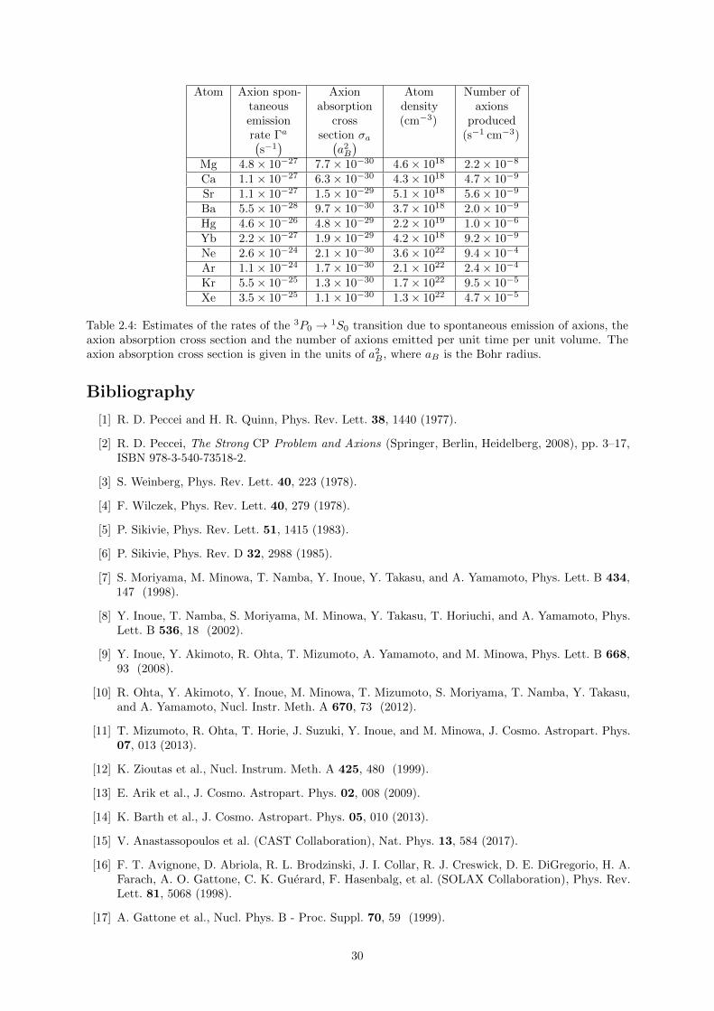
Atom Axion spon-taneousemissionrate Γa(

s−1)

Axionabsorption

crosssection σa(

a2B

)Atom

density(cm−3)

Number ofaxions

produced(s−1 cm−3)

Mg 4.8× 10−27 7.7× 10−30 4.6× 1018 2.2× 10−8

Ca 1.1× 10−27 6.3× 10−30 4.3× 1018 4.7× 10−9

Sr 1.1× 10−27 1.5× 10−29 5.1× 1018 5.6× 10−9

Ba 5.5× 10−28 9.7× 10−30 3.7× 1018 2.0× 10−9

Hg 4.6× 10−26 4.8× 10−29 2.2× 1019 1.0× 10−6

Yb 2.2× 10−27 1.9× 10−29 4.2× 1018 9.2× 10−9

Ne 2.6× 10−24 2.1× 10−30 3.6× 1022 9.4× 10−4

Ar 1.1× 10−24 1.7× 10−30 2.1× 1022 2.4× 10−4

Kr 5.5× 10−25 1.3× 10−30 1.7× 1022 9.5× 10−5

Xe 3.5× 10−25 1.1× 10−30 1.3× 1022 4.7× 10−5

Table 2.4: Estimates of the rates of the 3P0 → 1S0 transition due to spontaneous emission of axions, theaxion absorption cross section and the number of axions emitted per unit time per unit volume. Theaxion absorption cross section is given in the units of a2

B , where aB is the Bohr radius.

Bibliography

[1] R. D. Peccei and H. R. Quinn, Phys. Rev. Lett. 38, 1440 (1977).

[2] R. D. Peccei, The Strong CP Problem and Axions (Springer, Berlin, Heidelberg, 2008), pp. 3–17,ISBN 978-3-540-73518-2.

[3] S. Weinberg, Phys. Rev. Lett. 40, 223 (1978).

[4] F. Wilczek, Phys. Rev. Lett. 40, 279 (1978).

[5] P. Sikivie, Phys. Rev. Lett. 51, 1415 (1983).

[6] P. Sikivie, Phys. Rev. D 32, 2988 (1985).

[7] S. Moriyama, M. Minowa, T. Namba, Y. Inoue, Y. Takasu, and A. Yamamoto, Phys. Lett. B 434,147 (1998).

[8] Y. Inoue, T. Namba, S. Moriyama, M. Minowa, Y. Takasu, T. Horiuchi, and A. Yamamoto, Phys.Lett. B 536, 18 (2002).

[9] Y. Inoue, Y. Akimoto, R. Ohta, T. Mizumoto, A. Yamamoto, and M. Minowa, Phys. Lett. B 668,93 (2008).

[10] R. Ohta, Y. Akimoto, Y. Inoue, M. Minowa, T. Mizumoto, S. Moriyama, T. Namba, Y. Takasu,and A. Yamamoto, Nucl. Instr. Meth. A 670, 73 (2012).

[11] T. Mizumoto, R. Ohta, T. Horie, J. Suzuki, Y. Inoue, and M. Minowa, J. Cosmo. Astropart. Phys.07, 013 (2013).

[12] K. Zioutas et al., Nucl. Instrum. Meth. A 425, 480 (1999).

[13] E. Arik et al., J. Cosmo. Astropart. Phys. 02, 008 (2009).

[14] K. Barth et al., J. Cosmo. Astropart. Phys. 05, 010 (2013).

[15] V. Anastassopoulos et al. (CAST Collaboration), Nat. Phys. 13, 584 (2017).

[16] F. T. Avignone, D. Abriola, R. L. Brodzinski, J. I. Collar, R. J. Creswick, D. E. DiGregorio, H. A.Farach, A. O. Gattone, C. K. Guerard, F. Hasenbalg, et al. (SOLAX Collaboration), Phys. Rev.Lett. 81, 5068 (1998).

[17] A. Gattone et al., Nucl. Phys. B - Proc. Suppl. 70, 59 (1999).

30

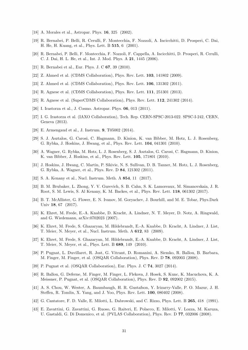
[18] A. Morales et al., Astropar. Phys. 16, 325 (2002).

[19] R. Bernabei, P. Belli, R. Cerulli, F. Montecchia, F. Nozzoli, A. Incicchitti, D. Prosperi, C. Dai,H. He, H. Kuang, et al., Phys. Lett. B 515, 6 (2001).

[20] R. Bernabei, P. Belli, F. Montecchia, F. Nozzoli, F. Cappella, A. Incicchitti, D. Prosperi, R. Cerulli,C. J. Dai, H. L. He, et al., Int. J. Mod. Phys. A 21, 1445 (2006).

[21] R. Bernabei et al., Eur. Phys. J. C 67, 39 (2010).

[22] Z. Ahmed et al. (CDMS Collaboration), Phys. Rev. Lett. 103, 141802 (2009).

[23] Z. Ahmed et al. (CDMS Collaboration), Phys. Rev. Lett. 106, 131302 (2011).

[24] R. Agnese et al. (CDMS Collaboration), Phys. Rev. Lett. 111, 251301 (2013).

[25] R. Agnese et al. (SuperCDMS Collaboration), Phys. Rev. Lett. 112, 241302 (2014).

[26] I. Irastorza et al., J. Cosmo. Astropar. Phys. 06, 013 (2011).

[27] I. G. Irastorza et al. (IAXO Collaboration), Tech. Rep. CERN-SPSC-2013-022. SPSC-I-242, CERN,Geneva (2013).

[28] E. Armengaud et al., J. Instrum. 9, T05002 (2014).

[29] S. J. Asztalos, G. Carosi, C. Hagmann, D. Kinion, K. van Bibber, M. Hotz, L. J. Rosenberg,G. Rybka, J. Hoskins, J. Hwang, et al., Phys. Rev. Lett. 104, 041301 (2010).

[30] A. Wagner, G. Rybka, M. Hotz, L. J. Rosenberg, S. J. Asztalos, G. Carosi, C. Hagmann, D. Kinion,K. van Bibber, J. Hoskins, et al., Phys. Rev. Lett. 105, 171801 (2010).

[31] J. Hoskins, J. Hwang, C. Martin, P. Sikivie, N. S. Sullivan, D. B. Tanner, M. Hotz, L. J. Rosenberg,G. Rybka, A. Wagner, et al., Phys. Rev. D 84, 121302 (2011).

[32] S. A. Kenany et al., Nucl. Instrum. Meth. A 854, 11 (2017).

[33] B. M. Brubaker, L. Zhong, Y. V. Gurevich, S. B. Cahn, S. K. Lamoreaux, M. Simanovskaia, J. R.Root, S. M. Lewis, S. Al Kenany, K. M. Backes, et al., Phys. Rev. Lett. 118, 061302 (2017).

[34] B. T. McAllister, G. Flower, E. N. Ivanov, M. Goryachev, J. Bourhill, and M. E. Tobar, Phys.DarkUniv 18, 67 (2017).

[35] K. Ehret, M. Frede, E.-A. Knabbe, D. Kracht, A. Lindner, N. T. Meyer, D. Notz, A. Ringwald,and G. Wiedemann, arXiv:0702023 (2007).

[36] K. Ehret, M. Frede, S. Ghazaryan, M. Hildebrandt, E.-A. Knabbe, D. Kracht, A. Lindner, J. List,T. Meier, N. Meyer, et al., Nucl. Instrum. Meth. A 612, 83 (2009).

[37] K. Ehret, M. Frede, S. Ghazaryan, M. Hildebrandt, E.-A. Knabbe, D. Kracht, A. Lindner, J. List,T. Meier, N. Meyer, et al., Phys. Lett. B 689, 149 (2010).

[38] P. Pugnat, L. Duvillaret, R. Jost, G. Vitrant, D. Romanini, A. Siemko, R. Ballou, B. Barbara,M. Finger, M. Finger, et al. (OSQAR Collaboration), Phys. Rev. D 78, 092003 (2008).

[39] P. Pugnat et al. (OSQAR Collaboration), Eur. Phys. J. C 74, 3027 (2014).

[40] R. Ballou, G. Deferne, M. Finger, M. Finger, L. Flekova, J. Hosek, S. Kunc, K. Macuchova, K. A.Meissner, P. Pugnat, et al. (OSQAR Collaboration), Phys. Rev. D 92, 092002 (2015).

[41] A. S. Chou, W. Wester, A. Baumbaugh, H. R. Gustafson, Y. Irizarry-Valle, P. O. Mazur, J. H.Steffen, R. Tomlin, X. Yang, and J. Yoo, Phys. Rev. Lett. 100, 080402 (2008).

[42] G. Cantatore, F. D. Valle, E. Milotti, L. Dabrowski, and C. Rizzo, Phys. Lett. B 265, 418 (1991).

[43] E. Zavattini, G. Zavattini, G. Ruoso, G. Raiteri, E. Polacco, E. Milotti, V. Lozza, M. Karuza,U. Gastaldi, G. Di Domenico, et al. (PVLAS Collaboration), Phys. Rev. D 77, 032006 (2008).

31

[44] F. Della Valle, A. Ejlli, U. Gastaldi, G. Messineo, E. Milotti, R. Pengo, G. Ruoso, and G. Zavattini,Eur. Phys. J. C 76, 24 (2016).

[45] S. J. Chen, H. H. Mei, and W. T. Ni, Mod. Phys. Lett. A 22, 2815 (2007).

[46] R. Battesti, B. Pinto Da Souza, S. Batut, C. Robilliard, G. Bailly, C. Michel, M. Nardone, L. Pinard,O. Portugall, G. Trenec, et al., Eur. Phys. J. D 46, 323 (2008).

[47] J. Jackel, A. Lindner, and J. Redondo, eds., Proceedings, 5th Patras Workshop on Axions, WIMPsand WISPs (AXION-WIMP 2009), DESY (DESY, Hamburg, Germany, 2010).

[48] L. Maiani, R. Petronzio, and E. Zavattini, Phys. Lett. B 175, 359 (1986).

[49] R. Barbieri, M. Cerdonio, G. Fiorentini, and S. Vitale, Phys. Lett. B 226, 357 (1989).

[50] R. Barbieri, C. Braggio, G. Carugno, C. Gallo, A. Lombardi, A. Ortolan, R. Pengo, G. Ruoso, andC. Speake, Phys. Dark Univ 15, 135 (2017).

[51] P. W. Graham and S. Rajendran, Phys. Rev. D 84, 055013 (2011).

[52] D. Budker, P. W. Graham, M. Ledbetter, S. Rajendran, and A. O. Sushkov, Phys. Rev. X 4, 021030(2014).

[53] P. W. Graham and S. Rajendran, Phys. Rev. D 88, 035023 (2013).

[54] Y. V. Stadnik and V. V. Flambaum, Phys. Rev. D 89, 043522 (2014).

[55] C. Abel et al., Phys. Rev. X 7, 041034 (2017).

[56] D. Horns, J. Jaeckel, A. Lindner, A. Lobanov, J. Redondo, and A. Ringwald, J. Cosmo. Astropart.Phys. 04, 016 (2013).

[57] J. Jaeckel and J. Redondo, Phys. Rev. D 88, 115002 (2013).

[58] A. J. Millar, G. G. Raffelt, J. Redondo, and F. D. Steffen, J. Cosmo. Astropart. Phys 01, 061(2017).

[59] A. Caldwell, G. Dvali, B. Majorovits, A. Millar, G. Raffelt, J. Redondo, O. Reimann, F. Simon,and F. Steffen (MADMAX Collaboration), Phys. Rev. Lett. 118, 091801 (2017).

[60] J. E. Moody and F. Wilczek, Phys. Rev. D 30, 130 (1984).

[61] A. Arvanitaki and A. A. Geraci, Phys. Rev. Lett. 113, 161801 (2014).

[62] Y. V. Stadnik, V. A. Dzuba, and V. V. Flambaum, Phys. Rev. Lett. 120, 013202 (2018).

[63] V. A. Dzuba, V. V. Flambaum, I. B. Samsonov, and Y. V. Stadnik, Phys. Rev. D 98, 035048(2018).

[64] Y. Kahn, B. R. Safdi, and J. Thaler, Phys. Rev. Lett. 117, 141801 (2016).

[65] G. Ruoso, A. Lombardi, A. Ortolan, R. Pengo, C. Braggio, G. Carugno, C. S. Gallo, and C. C.Speake, J. Phys. - Conf. Ser 718, 042051 (2016).

[66] Y. Hochberg, T. Lin, and K. M. Zurek, Phys. Rev. D 94, 015019 (2016).

[67] Y. Hochberg, T. Lin, and K. M. Zurek, Phys. Rev. D 95, 023013 (2017).

[68] P. Sikivie, N. Sullivan, and D. B. Tanner, Phys. Rev. Lett. 112, 131301 (2014).

[69] S. Chaudhuri, P. W. Graham, K. Irwin, J. Mardon, S. Rajendran, and Y. Zhao, Phys. Rev. D 92,075012 (2015).

[70] M. Silva-Feaver, S. Chaudhuri, H. M. Cho, C. Dawson, P. Graham, K. Irwin, S. Kuenstner, D. Li,J. Mardon, H. Moseley, et al., EEE Trans. Appl. Supercond 27, 1 (2017).

[71] C. Beck, Phys. Rev. Lett. 111, 231801 (2013).

32

[72] C. Beck, Phys. Dark Univ. 7-8, 6 (2015).

[73] H. Tam and Q. Yang, Phys. Lett. B 716, 435 (2012).

[74] A. Arvanitaki, S. Dimopoulos, and K. Van Tilburg, Phys. Rev. X 8, 041001 (2018).

[75] C. Braggio et al., eds., New detectors for axions (Turin, Italy, 2017).

[76] C. J. Cao and A. Zhitnitsky, Phys. Rev. D 96, 015013 (2017).

[77] M. Yoshimura and N. Sasao, arXiv:1710.11262 (2017).

[78] K. Zioutas and Y. Semertzidis, Phys. Lett. A 130, 94 (1988).

[79] P. Sikivie, Phys. Rev. Lett. 113, 201301 (2014).

[80] L. Santamaria, C. Braggio, G. Carugno, V. D. Sarno, P. Maddaloni, and G. Ruoso, New J. Phys.17, 113025 (2015).

[81] K. Van Bibber, N. R. Dagdeviren, S. E. Koonin, A. K. Kerman, and H. N. Nelson, Phys. Rev. Lett.59, 759 (1987).

[82] K. van Bibber, P. M. McIntyre, D. E. Morris, and G. G. Raffelt, Phys. Rev. D 39, 2089 (1989).

[83] R. Baehre, B. Doebrich, J. Dreyling-Eschweiler, S. Ghazaryan, R. Hodajerdi, D. Horns, F. Januschek,E. A. Knabbe, A. Lindner, D. Notz, et al., J. Instrum 8, T09001 (2013).

[84] V. B. Berestetskii, E. M. Lifshitz, and L. P. Pitaevskii, Quantum Electrodynamics, vol. 4 of Courseof Theoretical Physics (Pergamon Press, Oxford, 1982).

[85] K. Gottfried and T. M. Yan, Quantum mechanics: fundamentals (Springer, New York, Berlin,Heidelberg, 2013).

[86] I. I. Sobelman, Atomic spectra and radiative transitions, vol. 12 (Springer, New York, Berlin,Heidelberg, 2012).

[87] J. E. Kim, Phys. Rev. Lett. 43, 103 (1979).

[88] M. Shifman, A. Vainshtein, and V. Zakharov, Nucl. Phys. B 166, 493 (1980).

[89] M. Dine, W. Fischler, and M. Srednicki, Phys. Lett. B 104, 199 (1981).

[90] A. Zhitnitsky, Sov. J. Nucl. Phys. 31, 260 (1980).

[91] M. Srednicki, Nucl. Phys. B 260, 689 (1985).

[92] M. Pospelov, A. Ritz, and M. Voloshin, Phys. Rev. D 78, 115012 (2008).

[93] I. B. Khriplovich, Parity nonconservation in atomic phenomena (Gordon and Breach SciencePublishers, Philadelphia, 1991).

[94] O. Sushkov, V. Flambaum, and I. Khriplovich, Report at the Conference on the Theory of Atomsand Molecules (Vilnius, 1979).

[95] V. A. Dzuba, V. V. Flambaum, P. G. Silvestrov, and O. P. Sushkov, Phys. Rev. A 44, 2828 (1991).

[96] C. B. Alcock, V. P. Itkin, and M. K. Horrigan, Can. Metall. Q 23, 309 (1984).

[97] G. G. Raffelt, Phys. Lett. B 166, 402 (1986).

[98] J. Isern, E. Garcia-Berro, S. Torres, and S. Catalan, Astrophys. J. Lett. 682, L109 (2008).

[99] J. Isern, S. Catalan, E. Garcia-Berro, and S. Torres, J. Phys. Conf. Ser. 172, 012005 (2009).

[100] A. H. Corsico, L. G. Althaus, M. M. Bertolami, A. D. Romero, E. Garcia-Berro, J. Isern, and S. O.Kepler, Mon. Notices Royal Astron. Soc. 424, 2792 (2012).

[101] A. Corsico, L. Althaus, A. Romero, A. Mukadam, E. Garcia-Berro, J. Isern, S. Kepler, and M. Corti,J. Cosmo. Astropart. Phys. 2012, 010 (2012).

33

[102] N. Viaux, M. Catelan, P. B. Stetson, G. G. Raffelt, J. Redondo, A. A. R. Valcarce, and A. Weiss,Phys. Rev. Lett. 111, 231301 (2013).

[103] V. V. Flambaum, I. B. Samsonov, H. B. Tran Tan, and D. Budker, Phys. Rev. D 98, 095028 (2018).

[104] G. S. Ofelt, J. Chem. Phys. 38, 2171 (1963).

[105] K. Binnemans, Coord. Chem. Rev. 295, 1 (2015).

[106] R. L. Ahlefeldt, M. R. Hush, and M. J. Sellars, Phys. Rev. Lett. 117, 250504 (2016).

[107] Z. Bush, S. Barke, H. Hollis, G. Mueller, and D. Tanner (2017).

[108] S. G. Porsev, M. G. Kozlov, Y. G. Rakhlina, and A. Derevianko, Phys. Rev. A 64, 012508 (2001).

[109] A. Kramida et al. (NIST ASD Team), NIST Atomic Spectra Database (2017).

[110] R. E. Drullinger, M. M. Hessel, and E. W. Smith, J. Chem. Phys. 66, 5656 (1977).

[111] W. M. Haynes, CRC handbook of chemistry and physics (CRC press, Boca Raton, 2014).

34

Chapter 3

Coherent axion-photontransformations in the forwardscattering on atoms

3.1 Overview

In this chapter, I consider the possibility of producing axions by using forward scattering on atoms inmedia. Conventionally, axions are produced from photons in a strong magnetic field, with the photon-to-axion conversion rate being proportional to the axion-photon coupling gaγγ squared. In contrast, themechanism investigated in this chapter has a production rate which is proportional to the axion-electroncoupling gaee squared. Thus, this gives us a method to measure a different interaction constant.

This results is published in the following paper:

1. V. V. Flambaum, I. B. Samsonov, H. B. Tran Tan and D. Budker, Coherent axion-photontransformations in the forward scattering on atoms, Phys. Rev. D 98, 095028 (2018),arXiv:1805.01793,

which I presented at the international workshop:

1. Coherent axion-photon transformations in the forward scattering on atoms, QuantumTechnologies for Axion Dark Matter Detection Incubator, University of Sydney, Sydney, Australia,September 2018.

3.2 Abstract

In certain laboratory experiments the production and/or detection of axions is due to the photon-axiontransformations in a strong magnetic field. This process is coherent, and the rate of the transformationis proportional to the length l and magnitude B of the magnetic field squared, ∼ l2B2. In the presentpaper, we consider coherent production of axions due to the forward scattering of photons on atomsor molecules. This process may be represented as being due to an effective electromagnetic field whichconverts photons to axions. We present analytical expressions for such effective magnetic and electricfields induced by resonant atomic M0 and M1 transitions, as well as give some numerical estimates forthese fields. The corresponding experiments would allow one to measure the electron-axion couplingconstant gae in the same way as the photon-axion coupling gaγ is studied.

3.3 Introduction

The axion was introduced to explain the absence of CP violation in the strong interaction [1–9] and isconsidered as a probable candidate for a dark matter particle. The majority of experiments searchingfor axions in laboratories are based on the transformation of axions to photons (for axion detection)and photons to axions (for axion production) in a strong magnetic field [10–49]. The use of atomic andmolecular transitions for the axion detection has been suggested in Refs. [50–55]. It is natural to assume

35

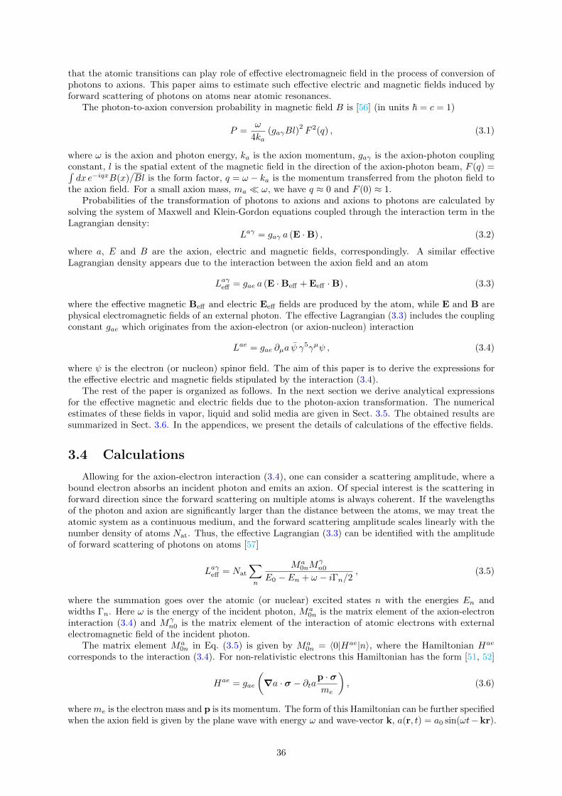
that the atomic transitions can play role of effective electromagneic field in the process of conversion ofphotons to axions. This paper aims to estimate such effective electric and magnetic fields induced byforward scattering of photons on atoms near atomic resonances.

The photon-to-axion conversion probability in magnetic field B is [56] (in units ~ = c = 1)

P =ω

4ka(gaγBl)

2F 2(q) , (3.1)

where ω is the axion and photon energy, ka is the axion momentum, gaγ is the axion-photon couplingconstant, l is the spatial extent of the magnetic field in the direction of the axion-photon beam, F (q) =∫dx e−iqxB(x)/Bl is the form factor, q = ω − ka is the momentum transferred from the photon field to

the axion field. For a small axion mass, ma ω, we have q ≈ 0 and F (0) ≈ 1.Probabilities of the transformation of photons to axions and axions to photons are calculated by

solving the system of Maxwell and Klein-Gordon equations coupled through the interaction term in theLagrangian density:

Laγ = gaγ a (E ·B) , (3.2)

where a, E and B are the axion, electric and magnetic fields, correspondingly. A similar effectiveLagrangian density appears due to the interaction between the axion field and an atom

Laγeff = gae a (E ·Beff + Eeff ·B) , (3.3)

where the effective magnetic Beff and electric Eeff fields are produced by the atom, while E and B arephysical electromagnetic fields of an external photon. The effective Lagrangian (3.3) includes the couplingconstant gae which originates from the axion-electron (or axion-nucleon) interaction

Lae = gae ∂µa ψ γ5γµψ , (3.4)

where ψ is the electron (or nucleon) spinor field. The aim of this paper is to derive the expressions forthe effective electric and magnetic fields stipulated by the interaction (3.4).

The rest of the paper is organized as follows. In the next section we derive analytical expressionsfor the effective magnetic and electric fields due to the photon-axion transformation. The numericalestimates of these fields in vapor, liquid and solid media are given in Sect. 3.5. The obtained results aresummarized in Sect. 3.6. In the appendices, we present the details of calculations of the effective fields.

3.4 Calculations

Allowing for the axion-electron interaction (3.4), one can consider a scattering amplitude, where abound electron absorbs an incident photon and emits an axion. Of special interest is the scattering inforward direction since the forward scattering on multiple atoms is always coherent. If the wavelengthsof the photon and axion are significantly larger than the distance between the atoms, we may treat theatomic system as a continuous medium, and the forward scattering amplitude scales linearly with thenumber density of atoms Nat. Thus, the effective Lagrangian (3.3) can be identified with the amplitudeof forward scattering of photons on atoms [57]

Laγeff = Nat

∑n

Ma0nM

γn0

E0 − En + ω − iΓn/2, (3.5)

where the summation goes over the atomic (or nuclear) excited states n with the energies En andwidths Γn. Here ω is the energy of the incident photon, Ma

0n is the matrix element of the axion-electroninteraction (3.4) and Mγ

n0 is the matrix element of the interaction of atomic electrons with externalelectromagnetic field of the incident photon.

The matrix element Ma0n in Eq. (3.5) is given by Ma

0n = 〈0|Hae|n〉, where the Hamiltonian Hae

corresponds to the interaction (3.4). For non-relativistic electrons this Hamiltonian has the form [51, 52]

Hae = gae

(∇a · σ − ∂ta

p · σme

), (3.6)

where me is the electron mass and p is its momentum. The form of this Hamiltonian can be further specifiedwhen the axion field is given by the plane wave with energy ω and wave-vector k, a(r, t) = a0 sin(ωt−kr).

36

Then the Hamiltonian may be represented in the form of multipole expansion with the leading termsgiven by (modulo the oscillating factor eiωt)

Hae = gae a0 (HaeM0 +Hae

M1 + . . .) , (3.7)

HaeM0 =

1

2

(− ω

mep · σ + i(k · r)(k · σ)

), (3.8)

HaeM1 = −1

2(k · σ) . (3.9)

The scattering amplitude (3.5) may be considered as a process, where an atom is (virtually) excitedby absorbing a photon and returns back to the initial state via axion emission. Note that the M0 axionsinduce transitions between the states of opposite atomic parity but the same total angular momentum.Thus, M0 axions are produced when atoms absorb E1 photon which also changes the parity. Analogously,M1 axions do not change parity, and they may be produced when M1 photons are absorbed. As a result,in Eq. (3.5) the matrix element of the operator Hae

M0 should be coupled with the matrix element of E1photon absorption operator Hγ

E1 = e(ε · r), while the matrix element of the operator HaeM1 should be

multiplied by the matrix element of M1 photon-absorption operator HγM1 = e

2me(n× ε)(J + S), where n

is the propagation unit vector of the photon and ε is its polarization. The former case corresponds tothe effective magnetic field while the latter generates the effective electric field due to the interaction ofphotons with atoms,

Beff = NatRe∑n

〈0|HaeM0|n〉〈n|H

γE1|0〉

E0 − En + ω − iΓn/2, (3.10)

Eeff = NatRe∑n

〈0|HaeM1|n〉〈n|H

γM1|0〉

E0 − En + ω − iΓn/2. (3.11)

The direction of the effective fields is specified by the matrix elements in Eqs. (3.10) and (3.11). Infact, as we prove in our previous paper [55], for non-polarized atoms the product of axion and photonmatrix elements always sums to zero,

∑n〈0|Hae|n〉〈n|Hγ |0〉 = 0, because the excited states |n〉 with

different projections of the total momentum contribute destructively. To get a non-vanishing result wehave to assume that a (weak) external magnetic field B2 is applied, which lifts the degeneracy of Zeemansublevels such that only some of them are in resonance with the applied laser field. In this case, it ispossible to show that the direction of the effective field Beff coincides with the direction of the appliedphysical magnetic field B2 while Eeff is directed along k×B2.

A resonant atomic transition may lead to a significant photon absorption and a phase shift of thephoton field (relative to the axions field) which destroys the coherence. Both effects may be seen fromthe complex phase in the photon field A ∝ einrk·r, where

nr = 1− 2πNat

∑n

|Mγn0|2

E0 − En + ω − iΓn/2(3.12)

is the complex refractive index. One could go to the tail of resonance to suppress the photon absorptionsince the imaginary part of nr decreases quadratically with E0 − En + ω, but the phase decreases slowly(linearly), similar to Eeff and Beff in Eqs. (3.10) and (3.11). The phase of the photons may be correctedby placing phase-correcting transparent plates in the medium. This situation is opposite to the case ofphoton-axion transformation in magnetic field [58], where it was proposed to use a gas to match thephotons’ speed with the speed of low-mass axion. In our case the phase-correcting transparent plates maybe needed if the photons’ phase velocity in the medium appears less than the axion’s speed. In this casethe plate should add the photons’ phase to equate the phase difference with axions to a multiple of 2π.

3.5 Numerical estimates

Note that the effective fields (3.10) and (3.11) are proportional to the atom density Nat. Thus, astronger effective field is produced in dense atomic systems such as solids, liquids or dense gases. In thisnote we consider noble gases in liquid phase and heavy metal vapors since they can be treated using thestandards atomic methods. We also show that there is a significant enhancements of the effective field incrystals with narrow spectral lines.

37

3.5.1 Effective magnetic field in liquid xenon

Let us consider liquid xenon with atomic density Nat = 1.3 × 1022 cm−3. The resonant axion M0transition is possible from the ground state 0+ to the excited state 0− with the energy E0− = 9.45 eV,while the corresponding photon transition is highly forbidden. This photon transition may be open whenan external magnetic field B2 is applied. This magnetic field causes the mixing of the states 0− and 1−,where the latter corresponds to the energy level E1− = 9.57 eV. As we demonstrate in Appendix 3.A.1,the effective magnetic field may reach the value

Beff ≈ 1.2× 10−2 T. (3.13)

We stress that, according to Eq. (3.3), the strength of interaction of this effective field with the axionfield is specified by the coupling constant gae, which is independent from the axion-photon constant gaγ .Thus, although this effective field is much weaker than the physical magnetic field B = 5.3 T appliedat the ALPS experiment [59], it may be significant in the processes of axion production or detection ifgae gaγ .

3.5.2 Effective electric field in vapor thallium

To estimate the effective electric field (3.11) we consider a vapor of Tl atoms at temperature T = 1200C and density Nat = 6.6×1017 cm−3. This system proved useful in the study of weak-interaction-inducedoptical activity of heavy-metal vapors [60]. Indeed, the transition between the ground state A with J = 1

2and the nearest excited state B with J = 3

2 is of M1 type. The energy difference between these statesω = 0.966 eV corresponds to near-infrared region. In Appendix 3.A.2 we give an estimate of the effectiveelectric field corresponding to such atomic transitions:

Eeff ≈ 1.5× 105 V

cm. (3.14)

This field is still not competitive with the physical magnetic field used at ALPS experiments.

3.5.3 Effective electric field in a crystal

According to equations (3.10) and (3.11), the strong effective fields are achieved in media with highatom density Nat and small width Γ. Therefore it is natural to consider photon-to-axion transformationsin crystals with narrow optical lines. One of such crystals based on EuCl3 · 6H2O compound has recentlybeen studied in [61]. Remarkable spectral properties of this crystal are due to the 4f valence electron shellof the Eu3+ ion [63, 64]. In particular, in [61] it was shown that the optical 7F0 → 5D0 transition in suchisotopically purified crystal may be as narrow as 25 MHz. However, we cannot employ this transitionfor axion production since it corresponds to the induced electric dipole type and does not obey theaxion-amplitude selection rules. Instead, we consider the transition 7F0 → 5D1 with the energy ω = 2.36eV in the Eu3+ ion, which is of M1 type [63] and is allowed for both the photon and axion amplitudes.Note that the states 7F0 and 5D1 refer to the intermediate coupling scheme, and each of them is given bya linear combination of the LS-states according to [64].

Although there is no explicit data about the width of the 7F0 → 5D1 transition in the EuCl3 · 6H2Ocrystal, we assume that it may be as narrow as for the 7F0 → 5D0 transition, Γ ∼ 10−7 eV. Then, takinginto account that the density of Eu atoms in this crystal is Nat ≈ 2.7 × 1021 cm−3 [61], in Appendix3.A.3 we estimate the effective electric field due to the photon-axion transformation:

Eeff ≈ 1.7× 109 V

cm. (3.15)

Thus, the effective field in crystals (3.15) is much stronger than that in vapor media (3.14) due to higheratom density and smaller linewidth.

We point out that Eq. (3.15) gives a rough estimate of the effective field because we do not know theexact width of the line corresponding to the 7F0 → 5D1 transition in the EuCl3 · 6H2O crystal. We hopethat a more accurate estimate may be given when this transition is experimentally measured.

3.6 Concluding remarks

The aim of this note is to attract the attention to the possibility to have resonance enhancement of theaxion-photon transformations in a medium. Such transitions between photons and axions in atoms can be

38

represented via the effective electric and/or magnetic fields, similar to the interaction of the axion withphysical electromagnetic fields. The crucial difference of these effective fields from the physical ones isthat they couple to the axion through the independent coupling constant gae which, for general axion-likeparticles, may be much larger than the axion-photon coupling gaγ . This motivates to set up new axionproduction/detection experiments where the medium plays the role of physical magnetic field in thecurrent axion-search experiments. Such new experiments would allow one to measure the axion-electroncoupling constant in the same way as the axion-photon coupling is studied. It is tempting to design suchexperiments and to estimate their efficiency.

We point out that the equations (3.10) and (3.11) give an important hint towards the design of futureatom- and molecule-based detectors with high sensitivity to axion-like particles: They should possessnarrow spectral lines at relatively high atom density. In particular, it is natural to look for crystals withultranarrow optical or microwave transitions. Examples of such crystals with the linewidth Γ ∼ 10−7 eVin the optical region have recently been studied, see, e.g., [61]. In Sect. 3.5.3 we demonstrated that theuse of such crystals as a media for photon-axion transformation may give a significant enhancement of theeffective field which may be much stronger than the physical fields employed at the ALPS experiments,see, e.g., [65] for a review. It is tempting to design such detectors and estimate their efficiency moreaccurately for applications in future ALPS experiments. We leave this issue for further work.

Acknowledgments

The authors thank R. Ahlefeldt, V. Dzuba, C. Rizzo, M. Sellars, and Y. Stadnik for useful discussions.This work is supported by the Australian Research Council, the Gutenberg Fellowship, New ZealandInstitute for Advanced Studies, the DFG via its Reinhardt Koselleck Program, and the European ResearchCouncil under the European Union’s Horizon 2020 Research 41 and Innovative Program under Grantagreement No. 695405.

3.A Estimates of effective fields

3.A.1 Effective magnetic field produced by liquid xenon

Let us consider the excited state 0− in Xe atom with energy E0− ≡ ω = 9.447 eV. This state haszero total angular momentum, J = 0, and odd parity in contrast with the even-parity ground state 0+.Therefore, the axion transition between these states is of M0 type. The corresponding matrix element forresonant axion absorption was calculated in our recent work [55]

Ma = 〈0−|HaeM0|0+〉 = i

√2

3ω2R , (3.16)

where R is the radial integral R =∫∞

0f6s1/2(r)f5p1/2(r)r3dr. Here f6s1/2(r) and f5p1/2(r) are radial parts

of 6s1/2 and 5p1/2 wavefunctions, respectively (see, e.g. [60]). For Xe atom, the value of this integral maybe deduced from [62], R ≈ −1.09 a.u.

The photon transition 0+ ↔ 0− is highly forbidden. However, this transition may be opened byapplying a magnetic field B2 which provides the mixing of the excited states |0−〉 and |1−〉,

|i〉 = |0−〉 − 〈1−|µ ·B2|0−〉E0− − E1−

|1−〉 , (3.17)

where E1− = 9.57 eV; µ = −µB(J + S) is the electron magnetic moment operator and µB is the Bohrmagneton. Taking into account that the matrix element 〈0−|µ · B2|1−〉 is 2/3µBB2, the photon E1transition amplitude between the ground state |0+〉 and the excited state |i〉 is found to be

Mγ =2

3

eµBB2

E0− − E1−〈1−|ε · r|0+〉 =

√2

9

eµBB2R

E0− − E1−, (3.18)

where ε is the photon polarization vector which is assumed to be along the z-axis, ε = (0, 0, 1). Thus, forthe product of transition amplitudes (3.16) and (3.18) we find

MaMγ =2i

27

eµBB2

E0− − E1−ω2R2 . (3.19)

39

Note that the expression (3.19) is imaginary. Hence, the real part of the effective Lagrangian (3.5)corresponds to the resonant absorption. Note also that for liquid Xe the dominant contribution to the widthof the state Γ comes from the collisional broadening, Γ ≈ Γcol = 2v0Natσcol, where v0 =

√2kBT/mat is

the most probable thermal speed of the atoms and σcol is the collisional cross section. Here kB is theBoltzmann constant and mat is the atomic mass. Assuming that the temperature of liquid Xe is T = 164K and the atom density is Nat = 1.3× 1022 cm−3, the collisional width is estimated as Γcol ≈ 1.4× 10−3

eV. Taking into account Eq. (3.19), we find the expression for the effective magnetic field

Beff =2

27Nat

µBB2

E0− − E1−

ω2R2

Γcol. (3.20)

Assuming that the magnetic field B2 is of order of the magnetic field applied at ALPS experiment[59], B2 = 5 T, we estimate the effective magnetic field produced by the atomic transitions (3.20):Beff ≈ 1.2× 10−2 T.

3.A.2 Effective electric field produced by thallium vapor

Consider the ground and excited states of the Tl atom, A = |L = 1, J = 12 〉 and B = |L = 1, J = 3

2 〉,with energy difference ω = 0.966 eV. The transition between these states is of M1 type. The axion andphoton absorption amplitudes for this transition are

Ma = −1

2〈B|k · σ|A〉 , (3.21)

Mγ =e

2me(n× ε)〈B|J + S|A〉 , (3.22)

where n is the photon or axion propagation unit vector and ε is the photon polarization vector. Forunpolarized atoms, in (3.11) we have to average over the states with different z-projection of the totalangular momentum MJ . After this averaging, the contribution to the effective electric field vanishes,∑MJ

MaMγ = 0, see [55].To get a non-vanishing result in (3.11) one can apply a magnetic field B2, which splits the Zeeman

sublevels. The laser frequency is in resonance with a transition from only one of these sublevels. Inparticular, we suppose that the constant magnetic field B2 is applied along the z-axis, B2 = B2z, andthe laser frequency corresponds to the energy difference of levels A = |1, 1

2 ,−12 〉 and B = |1, 3

2 ,12 〉. We

assume also that the photon propagates along the y-axis and is polarized in the (x, z)-plain, n = (0, 1, 0),ε = (εx, 0, εz). In this case, the axion and photon matrix elements (3.21) and (3.22) are

Ma =i

3√

2ωI , (3.23)

Mγ =eεzI

6√

2me

, (3.24)

where I is the overlap integral for 6p1/2 and 6p3/2 wavefunctions, I =∫∞

0dr r2f6p1/2(r)f6p3/2(r) ≈ 0.98.

As is shown in [60], for Tl vapor at a temperature of T = 1473 K, the dominant contribution to thewidth of the line comes from the Doppler broadening, Γ ≈ ΓDop = 2v0ω/

√π, where v0 =

√2kBT/mat is

the most probable thermal speed of the atoms. The numerical estimate for this width is ΓDop ≈ 1.3×10−6

eV. Taking this into account, we have the following expression for the effective electric field

Eeff = Nate

18me

ωI2εzΓDop

, (3.25)

where the density of the vapor is Nat = 6.6× 1017 cm−3.Assuming that the polarization of the photon is such that εz = 1, we estimate the effective electric

field Eeff ≈ 1.5× 105 Vcm .

Note that the same result may be obtained using the optical pumping rather than applying themagnetic field B2.

3.A.3 Effective electric field in crystals

Let us consider a EuCl3·6H2O crystal, where there are narrow spectral lines in the optical region, andhigh optical density can be achieved, see [61]. The optical properties of this crystal can be understood

40

through the electron-shell structure of the Eu3+ ion which has six valence electrons on the 4f orbital[63, 64]. We are interested in the transition between the states A = 7F0 and B = 5D1 corresponding tothe energy ω = 2.36 eV. Since this transition is of M1 type, we apply the formula (3.11) to estimate theeffective electric field Eeff due to axion-photon transformation.

The relevant computation is similar to the one given in Sect. 3.A.2 for Tl vapor. In particular, itis also necessary to apply the constant magnetic field B2 along the z-axis to lift the degeneracy of theZeeman sub-levels of state B = 5D1 with the total angular momentum J = 1. To be specific, we assumethat the laser frequency is in resonance with the transition between the states |A〉 = |7F0; J = 0,M = 0〉and |B〉 = |5D1; J = 1,M = 1〉. For simplicity, we also assume that the laser beam is aligned along they-direction and is polarized in the z-direction, so that n = (0, 1, 0) and ε = (0, 0, 1). In this case, usingthe equations (3.21) and (3.22) we find

Ma = − i√6ω〈5D1||S||7F0〉 , (3.26)

Mγ = − e

2√

6me

〈5D1||J + S||7F0〉 , (3.27)

where 〈5D1||S||7F0〉 is the reduced matrix element of the spin operator S and 〈5D1||J + S||7F0〉 =〈5D1||S||7F0〉. This matrix element may be computed using the spectral data for the Eu3+ ion [63, 64]:〈5D1||S||7F0〉 ≈ 0.17.

To apply the equation (3.11) we need the atom density Nat and the width of the state Γ. The formermay be easily estimated for the crystal EuCl3·6H2O described in [61]: Nat ≈ 2.7 × 1021 cm−3. Theauthors of this paper claim that the width of the optical transition 7F0 → 5D0 in this crystal is about 25MHz. For our estimates, we can assume that the transition 7F0 → 5D1 possesses a comparable widthΓ ∼ 10−7 eV. For these values of the parameters, we find the effective electric field in the crystal due tothe photon-axion transformation,

Eeff =Nateω

12meΓ|〈5D1||S||7F0〉|2 ≈ 1.7× 109 V

cm. (3.28)

We point out that these estimates are very rough; a more accurate estimate requires experimentalmeasurements of the width of the line for the transition 7F0 → 5D1 in the EuCl3·6H2O crystal.

Bibliography

[1] R. D. Peccei and H. R. Quinn, Phys. Rev. Lett. 38, 1440 (1977).

[2] R. D. Peccei, in Axions: Theory, Cosmology, and Experi-mental Searches (Springer, 2008) pp. 3-17.

[3] S. Weinberg, Phys. Rev. Lett. 40, 223 (1978).

[4] F. Wilczek, Phys. Rev. Lett. 40, 279 (1978).

[5] J. E. Kim, Phys. Rev. Lett. 43, 103 (1979).

[6] M. A. Shifman, A. I. Vainshtein and V. I. Zakharov, Nucl. Phys. B 166, 493 (1980).

[7] M. Dine, W. Fischler and M. Srednicki, Phys. Lett. 104B, 199 (1981).

[8] A. R. Zhitnitsky, Sov. J. Nucl. Phys. 31, 260 (1980) [Yad. Fiz. 31, 497 (1980)].

[9] M. Srednicki, Nucl. Phys. B 260, 689 (1985).

[10] P. Sikivie, Phys. Rev. Lett. 51, 1415 (1983) Erratum: [Phys. Rev. Lett. 52, 695 (1984)].

[11] P. Sikivie, Phys. Rev. D 32, 2988 (1985) Erratum: [Phys. Rev. D 36, 974 (1987)].

[12] S. Moriyama, M. Minowa, T. Namba, Y. Inoue, Y. Takasu and A. Yamamoto, Phys. Lett. B 434,147 (1998).

[13] Y. Inoue, T. Namba, S. Moriyama, M. Minowa, Y. Takasu, T. Horiuchi and A. Yamamoto, Phys.Lett. B 536, 18 (2002).

41

[14] Y. Inoue, Y. Akimoto, R. Ohta, T. Mizumoto, A. Yamamoto and M. Minowa, Phys. Lett. B 668, 93(2008).

[15] R. Ohta et al., Nucl. Instrum. Meth. A 670, 73 (2012).

[16] T. Mizumoto, R. Ohta, T. Horie, J. Suzuki, Y. Inoue and M. Minowa, JCAP 1307, 013 (2013).

[17] K. Zioutas et al., Nucl. Instrum. Meth. A 425, 480 (1999).

[18] E. Arik et al. [CAST Collaboration], JCAP 0902, 008 (2009).

[19] V. Anastassopoulos et al. [CAST Collaboration], Nature Phys. 13, 584 (2017).

[20] F. T. Avignone, III et al. [SOLAX Collaboration], Phys. Rev. Lett. 81, 5068 (1998).

[21] A. O. Gattone et al., Nucl. Phys. Proc. Suppl. 70, 59 (1999).

[22] A. Morales et al. [COSME Collaboration], Astropart. Phys. 16, 325 (2002).

[23] R. Bernabei et al., Phys. Lett. B 515, 6 (2001).

[24] R. Bernabei et al., Int. J. Mod. Phys. A 21, 1445 (2006).

[25] R. Bernabei et al. [DAMA and LIBRA Collaborations], Eur. Phys. J. C 67, 39 (2010).

[26] Z. Ahmed et al. [CDMS Collaboration], Phys. Rev. Lett. 103, 141802 (2009).

[27] Z. Ahmed et al. [CDMS-II Collaboration], Phys. Rev. Lett. 106, 131302 (2011).

[28] R. Agnese et al. [CDMS Collaboration], Phys. Rev. Lett. 111, no. 25, 251301 (2013).

[29] R. Agnese et al. [SuperCDMS Collaboration], Phys. Rev. Lett. 112, no. 24, 241302 (2014).

[30] I. G. Irastorza et al., JCAP 1106, 013 (2011).

[31] E. Armengaud et al., JINST 9, T05002 (2014).

[32] S. J. Asztalos et al. [ADMX Collaboration], Phys. Rev. Lett. 104, 041301 (2010).

[33] A. Wagner et al. [ADMX Collaboration], Phys. Rev. Lett. 105, 171801 (2010).

[34] J. Hoskins et al., Phys. Rev. D 84, 121302 (2011).

[35] S. Al Kenany et al., Nucl. Instrum. Meth. A 854, 11 (2017).

[36] B. M. Brubaker et al., Phys. Rev. Lett. 118, no. 6, 061302 (2017).

[37] B. T. McAllister et al., Phys. Dark Univ. 18, 67 (2017).

[38] K. Ehret et al., arXiv:0702023, (2007).

[39] K. Ehret et al. [ALPS Collaboration], Nucl. Instrum. Meth. A 612, 83 (2009).

[40] K. Ehret et al., Phys. Lett. B 689, 149 (2010).

[41] P. Pugnat et al. [OSQAR Collaboration], Phys. Rev. D 78, 092003 (2008).

[42] A. S. Chou et al. [GammeV (T-969) Collaboration], Phys. Rev. Lett. 100, 080402 (2008).

[43] G. Cantatore, F. Della Valle, E. Milotti, L. Dabrowski and C. Rizzo, Phys. Lett. B 265, 418 (1991).

[44] E. Zavattini et al. [PVLAS Collaboration], Phys. Rev. D 77, 032006 (2008).

[45] F. Della Valle, A. Ejlli, U. Gastaldi, G. Messineo, E. Milotti, R. Pengo, G. Ruoso and G. Zavattini,Eur. Phys. J. C 76, no. 1, 24 (2016).

[46] S. J. Chen, H. H. Mei and W. T. Ni, Mod. Phys. Lett. A 22, 2815 (2007).

[47] R. Battesti et al., Eur. Phys. J. D 46, 323 (2008).

42

[48] F. Bielsa et al., arXiv:0911.4567, (2009).

[49] E. Iacopini and E. Zavattini, Phys. Lett. 85B, 151 (1979).

[50] K. Zioutas and Y. Semertzidis, Phys. Lett. A 130, 94 (1988).

[51] P. Sikivie, Phys. Rev. Lett. 113, no. 20, 201301 (2014).

[52] M. Pospelov, A. Ritz and M. B. Voloshin, Phys. Rev. D 78, 115012 (2008).

[53] L. Santamaria et al., New J. Phys. 17, 113025 (2015).

[54] A. Arvanitaki, S. Dimopoulos and K. Van Tilburg, arXiv:1709.05354, (2017).

[55] H. B. Tran Tan, V. V. Flambaum, I. B. Samsonov, Y. V. Stadnik and D. Budker, arXiv:1803.09388,(2018).

[56] K. van Bibber, N. R. Dagdeviren, S. E. Koonin, A. Kerman and H. N. Nelson, Phys. Rev. Lett. 59,759 (1987).

[57] L. Landau and E. Lifshitz, Quantum Mechanics (Pergammon Press, Hungary, 1969)

[58] K. van Bibber, P. M. McIntyre, D. E. Morris, G. G. Raffelt, Phys. Rev. D 39, 2089 (1989).

[59] K. Ehret et al., Phys. Lett. B 689, 149 (2010).

[60] I. B. Khriplovich, Parity Nonconservation in Atomic Phenomena (Gordon and Breach, Amsterdam,1991).

[61] R. L. Ahlefeldt, M. R. Hush, and M. J. Sellars, Phys. Rev. Lett. 117, 250504 (2016).

[62] A. Kramida, Yu. Ralchenko, J. Reader and NIST ASD Team, NIST Atomic Spectra Database (ver.5.5.3), [Online]. Available: https://physics.nist.gov/asd [2018, March 31]. National Institute ofStandards and Technology, Gaithersburg, MD. (2018).

[63] K. Binnemans, Coord. Chem. Rev. 295, 1 (2015).

[64] G. S. Ofelt, J. Chem. Phys. 38, 2171 (1963).

[65] R. Battesti et al., arXiv:1803.07547 (2018).

43

Chapter 4

Screening and enhancement ofoscillating electric field in molecules

4.1 Overview

In this chapter, I consider the problem of screening of oscillating electric fields in molecules. It iswell-known that static electric fields do not penetrate to the nucleus of a neutral atom or molecule. Ishowed the oscillating electric field not only reaches the nucleus, but also may be enhanced by severalorders of magnitude if its frequency matches one of the atomic or molecular transition frequency. Thisfact is particularly useful for experiments detecting the CP -odd nuclear EDMs.

These results are published in the following paper:

1. H. B. Tran Tan, V. V. Flambaum and I. B. Samsonov, Screening and enhancement of anoscillating electric field in molecules, Phys. Rev. A 99, 013430 (2019), arXiv:1812.03312,

which I presented at one international conference, one international workshop and one nationalcompetition:

1. Searching for Axions and Axionic Dark Matter with Interference and Axion-inducedNuclear Moments, TeV Particle Astrophysics Conference, University of Sydney, Sydney, Australia,December 2019,

2. Screening and Enhancement of Nuclear Electric Dipole Moments Induced by AxionicDark Matter, Frontiers in Quantum Matter Workshop: Electric Dipole Moments, AustralianNational University, Canberra, Australia, November 2019,

3. Effects of Dark Matter in atomic and molecular phenomena, Australian Institute of PhysicsPostgraduate Presentation Competition, University of Technology Sydney, Sydney, Australia,October 2019.

4.2 Abstract

According to the Schiff theorem, the atomic electrons completely screen the atomic nucleus froman external static electric field. However, this is not the case if the field is time-dependent. Electronicorbitals in atoms either shield the nucleus from an oscillating electric field when the frequency of the fieldis off the atomic resonances or enhance this field when its frequency approaches an atomic transitionenergy. In molecules, not only electronic, but also rotational and vibrational states are responsible for thescreening of oscillating electric fields. As will be shown in this paper, the screening of a low-frequencyfield inside molecules is much weaker than it appears in atoms owing to the molecular ro-vibrationalstates. We systematically study the screening of oscillating electric fields inside diatomic molecules indifferent frequency regimes,i.e., when the field’s frequency is either of order of ro-vibrational or electronictransition frequencies. In the resonance case, we demonstrate that the microwave-frequency electricfield may be enhanced up to six orders in magnitude due to ro-vibrational states. We also derive thegeneral formulae for the screening and resonance enhancement of oscillating electric field in polyatomicmolecules. Possible applications of these results include nuclear electric dipole moment measurementsand stimulation of nuclear reactions by laser light.

44

4.3 Introduction

It is well-known that the Standard Model of elementary particles predicts small electric dipole moments(EDMs) for the electron and nucleon, see, e.g., Refs. [1–3] for recent reviews. Different extensions of SMsuch as axion or supersymmetry predict, however, different values for the EDMs of elementary particles.Therefore, it is a challenge for modern experimental physics to measure the EDMs of the electron andneutron in order to verify (or falsify) these models. Presently, there are several groups pursuing this goal,although the sensitivity of current experiments does not allow one to make firm conclusions.

One of the difficulties encountered in measuring the EDMs of nuclei in atoms and molecules is thescreening of the external electric field by the electron shells in these systems. Indeed, according to atheorem by Schiff [4], the atomic nucleus of a neutral atom is completely screened from any static externalelectric field. EDMs of diamagnetic atoms are produced by the interaction of electrons with the nuclearSchiff moment [5–9]. For light atoms, atomic EDMs produced by the Schiff moment are very small,while they appear significant for heavy atomic species (∼ 10−3dn; dn is the EDM of neutron). Thus, theelectron screening makes the detection of the nuclear EDMs difficult.

A possible way to overcome this difficulty is to use ions instead of neutral atoms, where the screeningof external fields is incomplete [10]. However, since a charged particle is not stationary in an electric field,it is problematic to preform precise measurements on such particle.

The behavior of atoms in an oscillating electric field is drastically different from that in the staticcase. It is natural to expect that the screening of alternating electric field in atoms and molecules isincomplete since the particles constituting an atom or a molecule respond to the changes in the field withsome delay. Recently, it has been shown that when the frequency of the external electric field is far fromatomic resonances, the resulting electric field at the center of an atom is proportional to the dynamicalatomic polarizability [11]. Numerical tests of these results were performed in Ref. [12]. However, whenthe frequency of the external field approaches the energy of atomic transition, there may be a significantenhancement (up to 105) of the field [13].

The extension of the static Schiff theorem to molecules was considered in Ref. [14]. The derivationtherein used the Ehrenfest theorem and resorted to classical mechanics to relate the acceleration ofeach nucleus to that of the whole molecule. Although this approach proved fruitful in the static case, itbecomes inefficient in the dynamic case since the classical motion of a molecule in an oscillating fieldis itself difficult to describe. This paper aims at developing a general and fully quantum mechanicalmethod for computing the electric field inside atoms and molecules which is applicable both for staticand oscillating electric fields.

Note that the quantum mechanical description of molecules has some important features as comparedwith the atomic case. In molecules, it is necessary to separate the relative motion of the constituentnuclei from the motion of the common center of mass while in atoms this separation is not essential, i.e.,the atomic nucleus may be considered as fixed in space. This relative motion of the nuclei in a moleculeis described by the rotational and vibrational modes. As a result, the molecular spectra appear to have avery rich structure with rotational, vibrational and electronic states. As will be shown in this paper, thesestates give rise to new terms in the formula for the resulting electric field in the molecule as comparedwith the atomic case studied in [11]. All these new terms play an important role in the screening of theexternal electric field in molecules.

The rest of this paper is organized as follows. In Sect. 4.4, the problem of calculating the field at thenuclei in a diatomic molecule in an external electric field is discussed. The cases of a static field, of anoscillating field off resonance with the molecular transitions and of an oscillating field on resonance with amolecular transition will be examined. In Sect. 4.5, we will consider examples of some diatomic moleculesand present the estimates of screening and resonance enhancement of electric field at nuclei. Sect. 4.6is devoted to the generalization of the diatomic-molecule case to systems of arbitrary number of nuclei.Sect. 4.7 contains a summary of the results and discussion of their potential application.

Throughout this paper, we employ the atomic units in which ~ = e = me = 4πε0 = 1. This makes theintermediate formulae more compact. The final results, for convenience, will be presented in arbitraryunits with all fundamental constants given explicitly.

4.4 Screening of electric field in diatomic molecules

In this section, we derive the general formulae for the screening of both static and alternating externalelectric fields inside diatomic molecules. To make our presentation self-consistent, we begin with a reviewof the molecular Hamiltonian in the center-of-mass coordinates frame.

45

4.4.1 The diatomic molecule Hamiltonian in the center-of-mass frame

Consider a diatomic molecule with L electrons in an external electric field Eext. Let MI and ZI be themasses and charges of the nuclei, respectively (the subscript I = 1, 2 labels the nuclei). The position andmomentum operators of the nuclei in the laboratory frame will be denoted by RI and PI , respectively.The electron positions and momenta operators will be denoted by ri and pi (the subscript i = 1, . . . , Llabels the electrons).

The Hamiltonian of the diatomic molecule in the laboratory frame has the standard form

Hmol = K + V0 + V , (4.1a)

K =P2

1

2M1+

P22

2M2+

L∑i=1

p2i

2, (4.1b)

V0 =Z1Z2

R12−

L∑i=1

(Z1

R1i+Z2

R2i

)+

L∑i<j

1

rij, (4.1c)

V = −Eext ·

(Z1R1 + Z2R2 −

L∑i=1

ri

), (4.1d)

where RIi = |RI − ri|, rij = |ri − rj | and RIJ = |RI −RJ |. Recall that we are using the atomic unitsystem in which e = me = 1. Here, for simplicity, we consider the non-relativistic Hamiltonian for spinlessparticles.

It is convenient to define the total nuclear mass MN = M1+M2, the total nuclear charge ZN = Z1+Z2,the total molecular mass MT = MN + L and the total molecular charge ZT = ZN − L (ZT = 0 for aneutral molecule).

To separate the molecule’s center-of-mass motion from the relative dynamics of the electrons andnuclei, we perform the change of variables (RI , ri)→ (ST ,S, si)

ST =1

MT

(M1R1 +M2R2 +

L∑i=1

ri

),

S = R1 −R2 ,

si = ri −M1R1 +M2R2

MN.

(4.2)

where ST is the position operator of the molecular center of mass, S defines the molecular axis and si arethe positions of the electrons with respect to the nuclear center of mass.

The conjugated momenta of the coordinates (ST ,S, si) will be denoted by (QT ,Q,qi). These momentaare related to the original momenta (PI ,pi) via

PI = −MI

MN

L∑i=1

qi − (−1)IQ +MI

MTQT ,

pi = qi +1

MTQT .

(4.3)

The change of variables (4.2) and (4.3) in the Hamiltonian (4.1) allows us to isolate the dynamics ofthe center-of-mass from the relative motion,

Hmol = HT +Hrel , (4.4)

where

HT =Q2T

2MT− ZTEext · ST (4.5)

is the center-of-mass Hamiltonian and Hrel is the Hamiltonian describing the relative dynamics

Hrel = H0 + Vrel , (4.6a)

H0 =

L∑i=1

q2i

2µe+

L∑i<j

qiqjMN

+Q2

2µN+ V0 , (4.6b)

Vrel = V + ZTEext · ST ≡ −d ·Eext . (4.6c)

46

Here

µN =M1M2

MN, µe =

MN

1 +MN(4.7)

are the reduced nuclear and electron masses, respectively, and d is the electric dipole moment with respectto the molecular center of mass,

d = −ζeL∑i=1

si + ζNS . (4.8)

Here we introduced the notations for the reduced electron charge ζe and reduced nuclear charge ζN :

ζe =MN + ZN

MT, (4.9)

ζN =M2Z1 −M1Z2

MN. (4.10)

Note that the Hamiltonian (4.6) contains the potential V0 defined in Eq. (4.1c). Here it is assumedthat this potential is expressed in terms of the new variables S and si.

We point out that this section presents no new results. It only describes the standard change ofvariables in the molecular Hamiltonian (4.1) which allows one to isolate the dynamics of the center ofmass of the molecule from the relative dynamics.

4.4.2 Screening of a static external electric field

Let us consider the screening of a static homogeneous electric field Eext = E0 at the position RI ofthe Ith nucleus. The operator of the electric field induced by the other nucleus and the electrons reads

E′I = − 1

ZI∇RI

V0 = − i

ZI[PI , H0] , (4.11)

where the Hamiltonian H0 is given in Eq. (4.6).Note that the Hamiltonian H0 defined in Eq. (4.6) is independent from the center-of-mass coordinate

ST . As a consequence, [QT , H0] = 0, and Eq. (4.11) may be put in the form

E′I = − i

ZI[ΠI , H0] , (4.12)

where ΠI denotes the truncated momentum operator

ΠI ≡ PI −MI

MTQT = −(−1)IQ− MI

MN

L∑i=1

qi . (4.13)

Using Eqs. (4.8) and (4.9), one can prove the following commutator relation between ΠI and thepotential Vrel given in Eq. (4.6c)(

1− MIZTMTZI

)E0 = − i

ZI[ΠI ,−d ·E0] . (4.14)

The composition of Eqs. (4.12) and (4.14) yields

E′I +

(1− MIZT

MTZI

)E0 = − i

ZI[ΠI , Hrel] . (4.15)

Let ψ be a stationary-state wavefunction describing the molecule in the center-of-mass frame, namely

Hrelψ = Eψ . (4.16)

The expectation value of the commutator on the right-hand side of Eq. (4.15) with respect to ψ vanishes.This allows us to find the expectation value of the operator E′I on the left-hand side of Eq. (4.15),〈E′I〉 ≡ 〈ψ|E′I |ψ〉, so the total electric field at Ith nucleus 〈EI〉 is

〈EI〉 ≡ 〈E′I〉+ E0 =MIZTMTZI

E0 . (4.17)

47

This result, derived in a fully quantum mechanical way, agrees with that obtained in Ref. [14] withthe use of the Ehrenfest theorem. Note that for a neutral molecule, ZT = 0 so the nuclei are completelyscreened from the static external field, 〈EI〉 = 0. In deriving this result we explicitly assumed that thenuclei are point-like particles. For real molecules, this screening is incomplete due to the finite-size effectsof the nuclei which are accounted for by the Schiff moment operator [5–9]. In this paper, however, we donot consider Schiff moment corrections.

4.4.3 Off-resonance screening of an oscillating external electric field

We now consider the case of an oscillating external electric field with frequency ω 1

Eext = E0 cosωt . (4.18)

When this field is sufficiently weak, the time-dependent perturbation theory may be applied to theHamiltonian (4.6) with

Vrel(t) = −d ·E0 cosωt (4.19)

treated as the perturbation.Let |n〉 be a complete set of eigenstates of the unperturbed Hamiltonian H0, namely

H0|n〉 = En|n〉 . (4.20)

Up to the first order in perturbation theory, the evolution of the ground state |0〉 is described by thewavefunction

ψ(t) = e−iE0t

[|0〉 − i

∑n

∫ t

dτ e−iωn0(t−τ)|n〉〈n|Vrel(τ)|0〉

], (4.21)

where ωn0 = En − E0. In this formula, we assume that the frequency of the external field ω is not inresonance with any transition with energy ωn0. In this case, it is safe to discard the widths of these states.The resonant case will be addressed in the next subsection.

Substituting the potential (4.19) into Eq. (4.21), we find the expectation value of the operator E′Idescribing the induced electric field at the Ith nucleus due to the other nucleus and the electrons,

〈E′I〉 ≡ 〈ψ(t)|E′I |ψ(t)〉 = 2 cosωt∑n

ωn0Re〈0|E′I |n〉〈n|d ·E0|0〉ω2n0 − ω2

. (4.22)

Making use of the identity (4.12), one may cast Eq. (4.22) in the form

〈E′I〉 =2 cosωt

ZI

∑n

ω2n0Im [〈0|ΠI |n〉〈n|d ·E0|0〉]

ω2n0 − ω2

, (4.23)

where the operator ΠI is defined as in Eq. (4.13).

Using the identityω2n0

ω2n0−ω2 = 1 + ω2

ω2n0−ω2 , the completeness of the set of states |n〉 and the relation

(4.15), we find the total electric field at the position of Ith nucleus

〈EI〉 ≡ 〈E′I〉+ E0 cosωt =MIZTMTZI

E0 cosωt+2ω2 cosωt

ZI

∑n

Im [〈0|ΠI |n〉〈n|d ·E0|0〉]ω2n0 − ω2

. (4.24)

We point out that Eq. (4.24) is valid not only for the Schrodinger Hamiltonian (4.6b), but also for thecase when the kinetic term for electrons is described by the Dirac Hamiltonian. In the latter case, therelativistic corrections due to the Dirac equation are included in the energies ωn0 and states |n〉.

Using the explicit form of the Hamiltonian H0 given in Eq. (4.6), one may prove the following identityfor the operator (4.13):

ΠI =iMI

ζeMT[−d +MIS, H0] , (4.25)

whereMI = (−1)I (MN −MI + ZN − ZI) , (4.26)

1An oscillating electric field Eext = E0 cosωt generates an oscillating magnetic field Bext = B0 cosωt where B0 isorthogonal to E0. This field however does not contribute to the resulting electric field at nuclei due to the parity selectionrules. Therefore in what follows we focus on the external electric field only.

48

and the quantities d and ζe are given in Eqs. (4.8) and (4.9), respectively.The identity (4.25) allows us to represent the formula (4.24) for the resulting electric field at the Ith

as

〈EI〉 =

[MIZTMTZI

− ω2MI

ζeMTZI

(↔α−

↔

βI

)]E0 cosωt , (4.27)

where↔α = 2

∑n

ωn0

ω2n0 − ω2

〈0|d|n〉〈n|d|0〉 (4.28)

is the molecule’s polarizability tensor and

↔

βI = 2MI

∑n

ωn0

ω2n0 − ω2

〈0|S|n〉〈n|d|0〉 . (4.29)

Eq. (4.27) describes the screening of an oscillating electric field inside a diatomic molecule in the casewhen the frequency of the field is off resonance from any molecular transition. Let us discuss the terms inthis formula.

The first term in the brackets has the same form as for the screening of static electric field (4.17).This term is proportional to the total charge of the molecule ZT which is vanishing for neutral molecules.

The second term in the brackets is specified by the molecular polarizability tensor↔α. This term has

the same structure as that in the formula for screening of electric fields in atoms derived in Ref. [11].

The last term in Eq. (4.27) is described by the tensor↔

βI defined in Eq. (4.29). This tensor dependson the matrix element of the inter-nuclear distance operator S which has no analogy in the atomic case.As we will show in the next section, this term plays a significant role in the screening of the external fieldin molecules. In fact, due to the large ratio of nuclear and electron mass |MI | ≈ (MN −MI) /me 1,↔

βI usually dominates over↔α. As will be discussed in Sect. 4.5.2, if the external field’s frequency is in

the rotational or vibrational regimes (10−5 − 10−3 a.u.) then |↔

βI | ↔α. Only the case where the field’s

frequency is in the electronic transition regime (∼ 0.1 a.u.) that↔

βI and↔α become comparable.

In conclusion of this section, we rewrite our results (4.27)–(4.29) with the fundamental constants ~, eand me explicitly shown

〈EI〉 =

[MIZTMTZI

− ω2meMI

e2ζeMTZI

(↔α−

↔

βI

)]Eext , (4.30a)

↔α =

2

~∑n

ωn0

ω2n0 − ω2

〈0|d|n〉〈n|d|0〉 , (4.30b)

↔

βI =2MI

~∑n

ωn0〈0|eS|n〉〈n|d|0〉ω2n0 − ω2

, (4.30c)

where MI = (−1)I[m−1e (MN −MI) + ZN − ZI

], ζe = M−1

T (MN +meZN ) and d = −ζeeL∑i=1

si + ζNeS.

Since me MI , one can make the (good) approximations ζe ≈ 1, M1 ≈ −M2/me, M2 ≈ M1/me

and MT ≈MN . Note that, with these approximations, the final term in the bracket in Eq. (4.30a) maybe written as

ω2meMI

e2ζeMTZI

↔

βI ≈2(−1)Iω2µN

e2~ZI

∑n

ωn0〈0|eS|n〉〈n|d|0〉ω2n0 − ω2

, (4.31)

where µN is the reduced nuclear mass defined in Eq. (4.7).

4.4.4 Resonance enhancement of an oscillating external electric field

When the frequency of the external electric field (4.18) approaches one of the molecular transitionfrequencies, ω = ωn0, the width of this state Γn cannot be ignored in perturbative calculations. In thiscase, the wavefunction (4.21) should be modified to read

ψ(t) = e−iE0t

[|0〉 − i

∑k

∫ t (dτe−i(ωk0−iΓk/2)(t−τ)|k〉〈k|Vrel(τ)|0〉

)]. (4.32)

49

Using the explicit form of the potential (4.19), we find the expectation value of the operator E′Idescribing the electric field at the Ith nucleus induced by the electrons and the other nucleus

〈E′I〉 =∑k

[− cos(ωt)fk(ω) +Γk2

sin(ωt)gk(ω)]Re〈0|E′I |k〉〈k| − d ·E0|0〉 , (4.33)

where

fk(ω) =ωk0 + ω

(ωk0 + ω)2 − (Γk/2)2+

ωk0 − ω(ωk0 − ω)2 − (Γk/2)2

, (4.34a)

gk(ω) =1

(ωk0 + ω)2 − (Γk/2)2− 1

(ωk0 − ω)2 − (Γk/2)2. (4.34b)

Note that in Eq. (4.33), we keep only the terms which are not suppressed by the small factor e−Γkt/2.It is natural to assume that all linewidths Γk are much smaller than the corresponding energies,

Γk ωk0. Under this assumption, the leading term in the functions fk (ω) and gk (ω) are

fk(ω) =

1/2ω , k = n2ωk0/

(ω2k0 − ω2

), k 6= n

, (4.35a)

gk(ω) =

−4/Γ2

n , k = n−4ωk0ω/(ω

2k0 − ω2)2 , k 6= n

. (4.35b)

Substituting these functions into Eq. (4.33) and using the identity (4.12), we find the total field atthe Ith nucleus 〈EI〉 ≡ E0 cos(ωt) + 〈E′I〉,

〈EI〉 =MIZTMTZI

E0 cosωt+2ω2 cosωt

ZI

∑k 6=n

Im [〈0|ΠI |k〉〈k|d ·E0|0〉]ω2k0 − ω2

− 3 cosωt

2ZIIm [〈0|ΠI |n〉〈n|d ·E0|0〉]−

2ω sinωt

ZIΓnIm [〈0|ΠI |n〉〈n|d ·E0|0〉] .

(4.36)

In deriving this result, we have employed the identity (4.14) and taken into account the completenessof the set of states |k〉.

Different terms in the expression (4.36) play different role in the screening or resonant enhancementof the electric field at the Ith nucleus in the molecule. Let us discuss them separately.

The term in the first line of Eq. (4.36) is present only for charged molecules with ZT 6= 0. In the restof this subsection we consider neutral molecules for which this term vanishes.

The term in the second line is responsible for the screening of the external field due to the stateswhich are off resonance with frequency ω. Strictly speaking, this term cannot be expressed via the tensors(4.30b) and (4.30c) since the sum does not contain the state |n〉, which is on resonance with the externalfield.

The terms in the last two lines arise from this state |n〉 which is in resonance with the external field.Between these terms, the last one dominates because the width is typically much smaller than the energy,Γn ω. Moreover, if |n〉 is a rotational or vibrational state then Γn is typically very small and the factorω/Γn in the last term of Eq. (4.36) makes it to dominate over all other terms. We can thus write (withthe constant e and me restored)

〈EI〉 ≈ω2meMI

ζee2ZIMTΓn

↔γIE0 sinωt , (4.37)

where we have introduced the tensor

↔γI = 2〈0|d|n〉〈n|d|0〉 − 2MI〈0|S|n〉〈n|d|0〉 . (4.38)

In deriving Eq. (4.37) we applied the identity (4.25).The electric field at the Ith nucleus (4.37) has the following features: (i) The external field may be

enhanced by many orders of magnitude due to the resonance factor ω/Γ. (ii) The phase of the resultingfield is shifted by π/2 with respect to the applied field. This is a typical resonance phase shift whichoccurs in damped driven oscillations. Both these features are already known for an atom in an oscillatingelectric field [13]. Here we establish similar results for molecules.

50

We note that although in the resonance case, the external field may be significantly enhanced thanksto the smallness of the width Γn, it certainly does not mean that one can induce an arbitrarily large fieldat a nucleus by using an arbitrarily strong external field. This is because for strong fields, perturbationtheory, in the framework of which the results of this section were derived, breaks down. The condition forthe applicability of perturbation theory reads

Ω Γn , (4.39)

where Ω ≡ |〈0|d ·E0|n〉| is the Rabi frequency (see Ref. [13] for more detail).If the condition Ω Γn is not met then 〈EI〉 may be calculated non-perturbatively by considering

the states |0〉 and |n〉 as forming a two-level quantum system. The result is

〈EI〉 ≈ω2meMI

ζee2ZIMT

ΓnΓ2n + 2Ω2

↔γIE0 sinωt . (4.40)

We note that for the weak external field E0 such that Ω Γn, Eq. (4.40) reduces to Eq. (4.37)derived perturbatively. For a strong external field such that Ω Γn the resulting electric field at nucleus〈EI〉 becomes inversely proportional to the applied field E0.

According to Eq. (4.40), the field 〈EI〉, considered as a function of E0 reaches its maximum at

E0 = Ecrit ≡Γn√2d

, (4.41)

where d = |〈0|d · k|n〉|. Here, k is the unit vector in the direction of E0. The maximal value of EI ≡ |〈EI〉|,corresponding to E0 = Ecrit is

EmaxI ≈ ω2meMI√

8ζee2ZIMT d|↔γI k| sinωt . (4.42)

It is important to note that this field is independent of the width of the excited state Γn.

4.5 Numerical estimates for diatomic molecules

In this section, the screening of an electric field in some diatomic molecules will be considered. To find

the total electric field at the Ith nucleus (4.27), one needs to evaluate the tensors↔α,

↔

βI and↔γI given

in Eqs. (4.28), (4.29) and (4.38). In general, to accurately compute these tensors one needs to applysophisticated numerical methods. Our goal is, however, to give crude semi-analytic estimates of someleading contributions to these tensors. For this purpose, we first develop a representation of these tensorsin the Born-Oppenheimer approximation and then present numerical estimates for some simple molecules.

4.5.1 Molecular polarizability in the Born-Oppenheimer approximation

The leading contributions to the tensors (4.28), (4.29) and (4.38) may be estimated in the Born-Oppenheimer approximation. In this approximation, the motion of the molecule in any state |n〉 maybe separated into rotational, vibrational and electronic modes. The rotational motion is described bythe Wigner D-matrix DJn

MnΛn(Θ) depending on the set of Euler angles Θ which describes the molecule’s

orientation with respect to the fixed laboratory frame (Jn is the molecule’s total angular momentumquantum number, Mn is the projection of this angular momentum onto the laboratory z-axis and Λn isthe projection of the electronic angular momentum onto the inter-nucler axis) whereas the vibrationaland electronic motions may be described by the ket |µnΛnνn〉 (νn is the vibrational quantum numberwhich, generally, depends on Jn, νn = νn(Jn), and µn denotes all other quantum numbers). We write

|n〉 =

√2Jn + 1

8π2DJnMnΛn

(Θ)|µnΛnνn〉 . (4.43)

where the coefficient√

(2Jn + 1) /8π2 is the normalization constant for the Wigner D-matrix. The ket|µnΛnνn〉 is assumed to be properly normalized.

The ket |µnΛnνn〉 may be considered as a wavefunction of the molecule in the rotating frame. Thiswavefunction factorizes into the vibrational ψµnΛn

νn (S) and electronic φµnΛn(S, si) parts,

|µnΛnνn〉 = S−1ψµnΛnνn (S)φµnΛn(S, si) . (4.44)

51

In this representation, we ignore all spins of electrons and nuclei. This approximation usually givesacceptable accuracy for low rotational levels [15].

In literature, the polarizablity tensor↔α is often calculated in the frame rotating with the molecule

(this frame is defined with respect to the laboratory by the angular coordinates Θ). However, the externalelectric field is naturally defined with respect to the laboratory frame. Thus, one needs to express thelaboratory-frame components of the molecular polarizability tensor via its rotating-frame components.

The spherical components of the vector d in the laboratory (l) and rotating (r) frames will be denoted

by d(l)q and d

(r)q (q = 0,±1), respectively. They are related to each other by the formula [15]

d(l)p =

∑q

(−1)p−q

D1pq(Θ)d(r)

q . (4.45)

This formula, together with Eq. (4.43) and the standard identity for the Wigner D-matrices [16, 17]

1

8π2

∫DJ′

M ′Λ′(Θ)Djpq(Θ)DJ

MΛ(Θ)dΘ = (−1)2J′−M ′−Λ′

(J ′ j J−M ′ p M

)(J ′ j J−Λ′ q Λ

), (4.46)

allows us to relate the laboratory-frame components of the tensor 〈0|d|n〉〈n|d|0〉 to its rotating-framecomponents

〈0|d(l)p |n〉〈n|d(l)

q |0〉 = δpq (2J0 + 1) (2Jn + 1)

×(

J0 1 Jn−M0 p Mn

)2(J0 1 Jn−Λ0 Λ0 − Λn Λn

)2 ∣∣∣〈µ0Λ0ν0|d(r)Λ0−Λn

|µnΛnνn〉∣∣∣2 . (4.47)

If the molecule is non-polarized in the ground state, the expression (4.47) should be averaged over thequantum number M0 and summed over the quantum number Mn. In this case, the molecular polarizabilitytensor (4.28) has only the scalar part α(ω), namely

↔α(ω) = α(ω)13×3 . (4.48)

Physically, this implies that the induced electric field in the non-polarized molecule can only be parallelto the external electric field.

Without loss of generality, it may be assumed that the external field Eext is directed along thelaboratory z-axis. For simplicity, it will also be assumed that the ground state is in the Σ (Λ = 0)configuration and has total angular momentum J0 = 0 (this assumption forces M0 = 0 and Jn = 1).Under these assumptions, the only relevant component of the tensor (4.47) is

〈0|d(l)0 |n〉〈n|d

(l)0 |0〉 = δ0Mn

(0 1 10 −Λn Λn

)2 ∣∣∣〈µ0Σν0|d(r)−Λn|µnΛnνn〉

∣∣∣2 , (4.49)

where the vibrational quantum number ν0 corresponds to the total momentum quantum number J = 0whereas νn is attributed to J = 1.

Substituting Eq. (4.49) into Eq. (4.28), we obtain the expression for the polarizability tensor in thelaboratory frame via the components of this tensor in the molecular (rotating) frame

α(ω) =1

3

[α‖el(ω) + 2α⊥el(ω) + α

‖vib(ω) + α

‖rot(ω)

], (4.50)

where α‖el and α⊥el are the parallel and perpendicular components with respect to the molecular axis

arising due to electronic excitations; α‖vib and α

‖rot are the terms originating from the vibrational and

rotational states. Explicitly, these quantities read

α‖el(ω) =

∑µn 6=µ0νn

2ωn0

ω2n0 − ω2

∣∣∣〈µ0Σν0| d(r)0 |µnΣνn〉

∣∣∣2, (4.51a)

α⊥el(ω) =∑µn,νn

2ωn0

ω2n0 − ω2

∣∣∣〈µ0Σν0| d(r)−1 |µnΠνn〉

∣∣∣2, (4.51b)

α‖vib(ω) =

∑νn 6=ν0

2ωn0

ω2n0 − ω2

∣∣∣〈µ0Σν0| d(r)0 |µ0Σνn〉

∣∣∣2, (4.51c)

α‖rot(ω) =

2ων0ν′0ω2ν0ν′0− ω2

∣∣∣〈µ0Σν0| d(r)0 |µ0Σν′0〉

∣∣∣2, (4.51d)

52

where the vibrational quantum numbers ν0 and ν′0 correspond to J = 0 and J = 1, respectively.As we will show in the end of this section, the representation for the molecular polarizablity (4.50)

appears useful, as the values of the quantities (4.51) may be either easily calculated or found in literature.Similar representations may be developed for the tensors (4.29) and (4.38). Following the same procedureas above, it is possible to prove that each of these tensors is proportional to the unit matrix,

↔

βI(ω) = βI(ω)13×3 ,↔γI(ω) = γI(ω)13×3 . (4.52)

For the quantity βI(ω) we find

βI(ω) =MI

3

[β‖vib(ω) + β

‖rot(ω)

], (4.53)

where

β‖vib(ω) = 2

∑νn 6=ν0

ωn0

ω2n0 − ω2

〈µ0Σν0|S |µ0Σνn〉 〈µ0Σνn| d(r)0 |µ0Σν0〉 , (4.54a)

β‖rot(ω) =

2ων0ν′0ω2ν0ν′0− ω2

〈µ0Σν0|S |µ0Σν′0〉 〈µ0Σν′0| d(r)0 |µ0Σν0〉 . (4.54b)

In contrast to the quantities (4.28) and (4.29), there is no summation over states in the formula of theγ-tensor (4.38) since only one pair of states is in resonance with the external field.

It is of interest to consider the external electric field in resonance with the lowest rotational state. Inthis case, we have

γI(ω) =2

3

∣∣∣〈µ0Σν0| d(r)0 |µ0Σνn〉

∣∣∣2 − 2

3MI 〈µ0Σν0|S |µ0Σνn〉 〈µ0Σνn| d(r)

0 |µ0Σν0〉 . (4.55)

In this formula, the second term on the right-hand side dominates over the first one since |MI | 1,

γI(ω) ≈ −2

3MI 〈µ0Σν0|S |µ0Σνn〉 〈µ0Σνn| d(r)

0 |µ0Σν0〉 . (4.56)

We point out, however, that the first term in Eq. (4.55) cannot be ignored if the external electric fieldis in resonance with electronic transitions in the molecule. In this case, the second term in Eq. (4.55)vanishes so the sole contribution to γI (ω) comes from its first term.

4.5.2 Screening of the external electric field in different frequency regimes

Recall that the molecular spectra have three typical frequency scales: ωrot associated with therotational transitions, ωvib associated with the vibrational transitions and ωel associated with theelectronic transitions. Normaly, ωrot ωvib ωel. It is interesting to consider the screening of externalelectric fields with frequencies in these three different regimes.

As was shown in the previous subsection, the induced electric field at the Ith nucleus is parallel to theexternal electric field. The magnitude of this field may be written as

EI = σI(ω)E0 cosωt , (4.57)

where the suppression factor σI is defined as

σI(ω) =MIZTMTZI

− ω2MI

ζeMTZI[α(ω)− βI(ω)] . (4.58)

The first term here is ω-independent and is non-vanishing only for charged molecules. Although this termis important in the total formula for the suppression factor, it is more interesting to analyze the otherterms in Eq. (4.58) which are non-vanishing both for charged and neutral molecules and are ω-dependent.Therefore, to the end of this subsection we will restrict ourselves to the case ZT = 0. We will also workin the limit me MI in which ζe ≈ 1, MI ≈ (−1)I (MN −MI) and MT ≈MN .

53

Screening of rotational-range-frequency fields

Let us consider an external electric field with frequency of order of the lowest rotational transitionfrequencies, ω ∼ ων0ν′0 . In this case, because the factor ωn0/

(ω2n0 − ω2

)in Eq. (4.28) scales as energy

inverse, the dominant contribution to α(ω) comes from Eq. (4.51d) and the dominant contribution to

βI(ω) comes from Eq. (4.54b). Since the matrix elements 〈µ0Σν0|S |µ0Σν′0〉 and 〈µ0Σν0| d(r)0 |µ0Σν′0〉 are

of the same order, and since |MI | 1, the dominant contribution to the suppression factor (4.58) comesfrom βI(ω). Thus, the leading contribution to the suppression factor (4.58) is given by the term (4.54b),namely

σrotI (ω) ≈ (−1)

I 2ω2µN3ZI

ωSd

ω2 − ω2, (4.59)

where

ω ≡ ων0ν′0 =1

µN S2(4.60)

is the rotational energy with J = 1,S = 〈µ0Σν0|S |µ0Σν0〉 (4.61)

is the ground state mean inter-nuclear distance and

d = 〈µ0Σν0| d(r)0 |µ0Σν0〉 (4.62)

is the ground state mean electric dipole (in the direction of S). Note that we have invoked the rigid-rotorapproximation which allows us to replace ν′0 by ν0 in the definition of S and d. We have also made theapproximation MIMI/MT ≈ (−1)IµN .

Screening of vibrational-range-frequency fields

In the case where ω is of the order of a vibrational energy, ω ∼ ωvib, contributions to α(ω) from α‖el

and α⊥el are negligible whereas the terms α‖vib and α

‖rot are significant. In the expression (4.53) for βI ,

both terms β‖vib and β

‖rot contribute. Again, since |MI | 1, βI dominates over α. Thus, in this case, the

leading contributions to the suppression factor (4.58) are

σI(ω) = σvibI (ω) + σrot

I (ω) , (4.63a)

σvibI (ω) ≈ (−1)

I 2ω2µN3ZI

∑νn 6=ν0

ωn0Sνnν0 (dr0)

ν0νn

ω2n0 − ω2

, (4.63b)

where ω, S and d are given in Eqs. (4.60), (4.61) and (4.62), respectively, and the quantities Sνnν0 and (dr0)are defined by

Sνnν0 = 〈µ0Σν0|S |µ0Σνn〉 (4.64)

and(dr0)

ν0νn

= 〈µ0Σνn| d(r)0 |µ0Σν0〉 . (4.65)

The quantity σrotI (ω) in Eq. (4.63a) is defined in Eq. (4.59). Note, however, that since the field’s

frequency, being in the vibrational regime, is much larger than the rotational frequency, we haveω2ωω2−ω2 ≈ −ω. As a result, this term σrot

I (ω) becomes independent of ω.The quantity Sνnν0 may be roughly estimated assuming that the vibrational mode is purely harmonic,

i.e., vibrational wavefunctions are harmonic oscillator wavefunctions. The operator d(r)0 may be written

as −∑Li=1 s

‖i + ζNS where s

‖i is the projection of si onto the molecular axis. The quantity (dr0)

ν0νn

may be approximated by −fν0νn s‖ + ζNS

ν0νn where fν0νn = 〈νn|ν0〉 is the Franck-Condon factor and s‖ =

〈µ0Σ|∑Li=1 s

‖i |µ0Σ〉. If one takes, approximately, fν0νn ≈ δν0νn then the electronic part drops out when

summed over all νn 6= ν0. In this case, (dr0)ν0νn≈ ζNSν0νn . Typically, Sν0νn decreases rapidly as νn increases.

Thus, only the term with νn = ν0 ± 1 makes dominant contribution to the sum in Eq. (4.63).

54

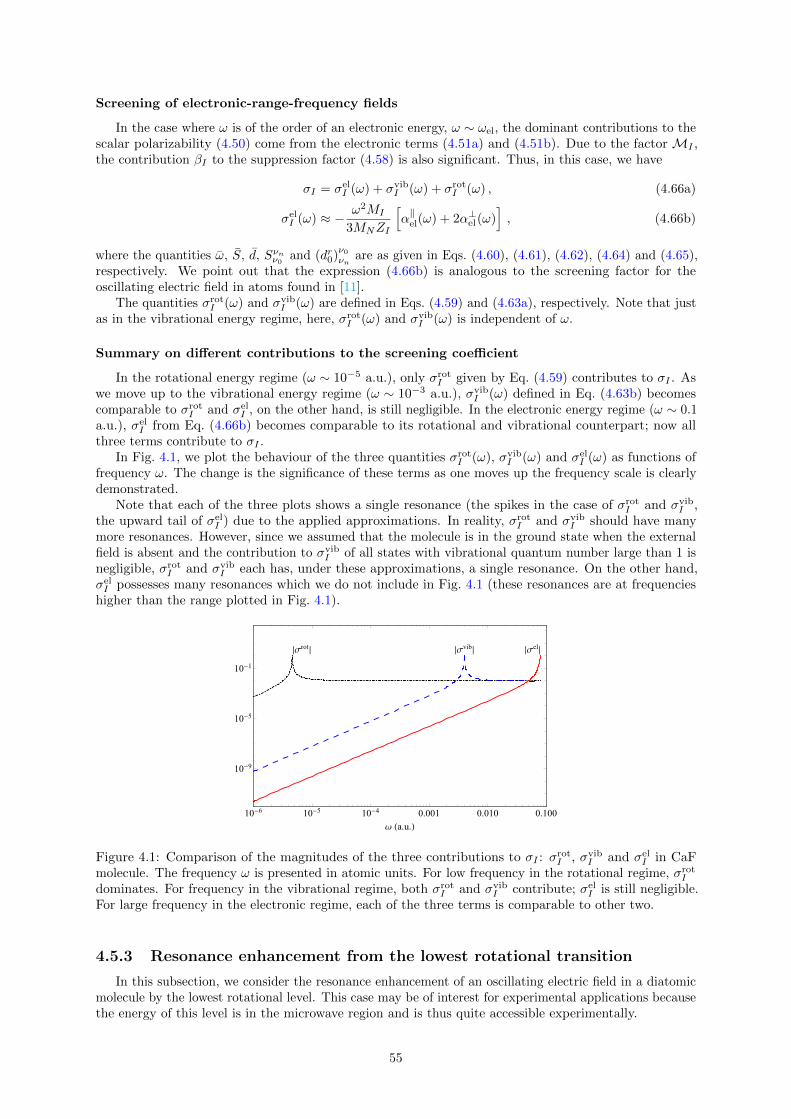
Screening of electronic-range-frequency fields

In the case where ω is of the order of an electronic energy, ω ∼ ωel, the dominant contributions to thescalar polarizability (4.50) come from the electronic terms (4.51a) and (4.51b). Due to the factor MI ,the contribution βI to the suppression factor (4.58) is also significant. Thus, in this case, we have

σI = σelI (ω) + σvib

I (ω) + σrotI (ω) , (4.66a)

σelI (ω) ≈ − ω2MI

3MNZI

[α‖el(ω) + 2α⊥el(ω)

], (4.66b)

where the quantities ω, S, d, Sνnν0 and (dr0)ν0νn

are as given in Eqs. (4.60), (4.61), (4.62), (4.64) and (4.65),respectively. We point out that the expression (4.66b) is analogous to the screening factor for theoscillating electric field in atoms found in [11].

The quantities σrotI (ω) and σvib

I (ω) are defined in Eqs. (4.59) and (4.63a), respectively. Note that justas in the vibrational energy regime, here, σrot

I (ω) and σvibI (ω) is independent of ω.

Summary on different contributions to the screening coefficient

In the rotational energy regime (ω ∼ 10−5 a.u.), only σrotI given by Eq. (4.59) contributes to σI . As

we move up to the vibrational energy regime (ω ∼ 10−3 a.u.), σvibI (ω) defined in Eq. (4.63b) becomes

comparable to σrotI and σel

I , on the other hand, is still negligible. In the electronic energy regime (ω ∼ 0.1a.u.), σel

I from Eq. (4.66b) becomes comparable to its rotational and vibrational counterpart; now allthree terms contribute to σI .

In Fig. 4.1, we plot the behaviour of the three quantities σrotI (ω), σvib

I (ω) and σelI (ω) as functions of

frequency ω. The change is the significance of these terms as one moves up the frequency scale is clearlydemonstrated.

Note that each of the three plots shows a single resonance (the spikes in the case of σrotI and σvib

I ,the upward tail of σel

I ) due to the applied approximations. In reality, σrotI and σvib

I should have manymore resonances. However, since we assumed that the molecule is in the ground state when the externalfield is absent and the contribution to σvib

I of all states with vibrational quantum number large than 1 isnegligible, σrot

I and σvibI each has, under these approximations, a single resonance. On the other hand,

σelI possesses many resonances which we do not include in Fig. 4.1 (these resonances are at frequencies

higher than the range plotted in Fig. 4.1).

|σrot| |σvib| |σel|

10-6 10-5 10-4 0.001 0.010 0.100

10-9

10-5

10-1

ω (a.u.)

Figure 4.1: Comparison of the magnitudes of the three contributions to σI : σrotI , σvib

I and σelI in CaF

molecule. The frequency ω is presented in atomic units. For low frequency in the rotational regime, σrotI

dominates. For frequency in the vibrational regime, both σrotI and σvib

I contribute; σelI is still negligible.

For large frequency in the electronic regime, each of the three terms is comparable to other two.

4.5.3 Resonance enhancement from the lowest rotational transition

In this subsection, we consider the resonance enhancement of an oscillating electric field in a diatomicmolecule by the lowest rotational level. This case may be of interest for experimental applications becausethe energy of this level is in the microwave region and is thus quite accessible experimentally.

55

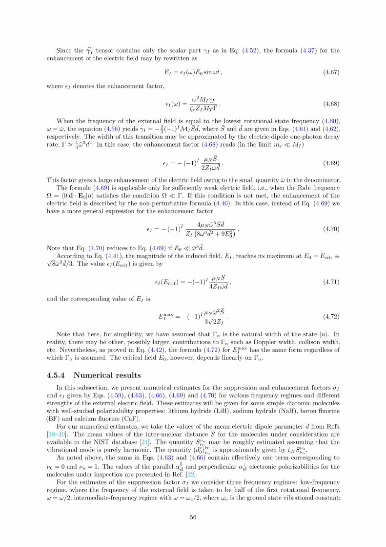
Since the↔γI tensor contains only the scalar part γI as in Eq. (4.52), the formula (4.37) for the

enhancement of the electric field may by rewritten as

EI = εI(ω)E0 sinωt , (4.67)

where εI denotes the enhancement factor,

εI(ω) =ω2MIγIζeZIMTΓ

. (4.68)

When the frequency of the external field is equal to the lowest rotational state frequency (4.60),ω = ω, the equation (4.56) yields γI = − 2

3 (−1)IMI Sd, where S and d are given in Eqs. (4.61) and (4.62),respectively. The width of this transition may be approximated by the electric-dipole one-photon decayrate, Γ ≈ 4

3 ω3d2. In this case, the enhancement factor (4.68) reads (in the limit me MI)

εI = − (−1)I µN S

2ZI ωd. (4.69)

This factor gives a large enhancement of the electric field owing to the small quantity ω in the denominator.The formula (4.69) is applicable only for sufficiently weak electric field, i.e., when the Rabi frequency

Ω = 〈0|d · E0|n〉 satisfies the condition Ω Γ. If this condition is not met, the enhancement of theelectric field is described by the non-perturbative formula (4.40). In this case, instead of Eq. (4.69) wehave a more general expression for the enhancement factor

εI = − (−1)I 4µN ω

5Sd

ZI(8ω6d2 + 9E2

0

) . (4.70)

Note that Eq. (4.70) reduces to Eq. (4.69) if E0 ω3d.According to Eq. (4.41), the magnitude of the induced field, EI , reaches its maximum at E0 = Ecrit ≡√

8ω3d/3. The value εI(Ecrit) is given by

εI(Ecrit) = −(−1)IµN S

4ZI ωd, (4.71)

and the corresponding value of EI is

EmaxI = −(−1)I

µN ω2S

3√

2ZI. (4.72)

Note that here, for simplicity, we have assumed that Γn is the natural width of the state |n〉. Inreality, there may be other, possibly larger, contributions to Γn such as Doppler width, collison width,etc. Nevertheless, as proved in Eq. (4.42), the formula (4.72) for Emax

I has the same form regardless ofwhich Γn is assumed. The critical field E0, however, depends linearly on Γn.

4.5.4 Numerical results

In this subsection, we present numerical estimates for the suppression and enhancement factors σIand εI given by Eqs. (4.59), (4.63), (4.66), (4.69) and (4.70) for various frequency regimes and differentstrengths of the external electric field. These estimates will be given for some simple diatomic moleculeswith well-studied polarizability properties: lithium hydride (LiH), sodium hydride (NaH), boron fluorine(BF) and calcium fluorine (CaF).

For our numerical estimates, we take the values of the mean electric dipole parameter d from Refs.[18–20]. The mean values of the inter-nuclear distance S for the molecules under consideration areavailable in the NIST database [21]. The quantity Sνnν0 may be roughly estimated assuming that thevibrational mode is purely harmonic. The quantity (dr0)

ν0νn

is approximately given by ζNSν0νn .

As noted above, the sums in Eqs. (4.63) and (4.66) contain effectively one term corresponding to

ν0 = 0 and νn = 1. The values of the parallel α‖el and perpendicular α⊥el electronic polarizabilities for the

molecules under inspection are presented in Ref. [22].For the estimates of the suppression factor σI we consider three frequency regimes: low-frequency

regime, where the frequency of the external field is taken to be half of the first rotational frequency,ω = ω/2; intermediate-frequency regime with ω = ωe/2, where ωe is the ground state vibrational constant;

56

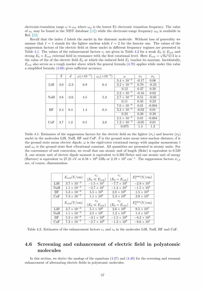
electronic-transition range ω ≈ ωel where ωel is the lowest E1 electronic transition frequency. The valueof ωe may be found in the NIST database [21]) while the electronic-range frequency ωel is available inRef. [22].

Recall that the index I labels the nuclei in the diatomic molecule. Without loss of generality weassume that I = 1 stands for the lighter nucleus while I = 2 for the heavier one. The values of thesuppression factors of the electric field at these nuclei in different frequency regimes are presented inTable 4.1. The values of the enhancement factors ε1 are given in Table 4.2 for a weak E0 Ecrit andstrong E0 = Ecrit external field in resonance with the first rotational level. Here Ecrit =

√8ω3d/3 is a

the value of the of the electric field E0 at which the induced field EI reaches its maxium. Incidentally,Ecrit also serves as a rough marker above which the general formula (4.70) applies while under this valuea simplified formula (4.69) gives sufficient accuracy.

S d ω(×10−5) ωe(×10−3) ω σ1 σ2

LiH 3.0 -2.3 6.9 6.43.4× 10−5 -0.17 0.063.2× 10−3 0.70 -0.23

0.12 0.37 0.20

NaH 3.6 -2.6 4.5 5.32.2× 10−5 -0.16 0.022.7× 10−3 0.51 -0.05

0.11 0.35 0.23

BF 2.4 0.4 1.4 6.47.0× 10−6 0.01 -0.0043.2× 10−3 -0.02 0.01

0.22 0.38 0.38

CaF 3.7 1.2 0.5 2.62.5× 10−6 0.01 -0.0041.3× 10−3 -0.05 0.01

0.075 1.4 1.3

Table 4.1: Estimates of the suppression factors for the electric field on the lighter (σ1) and heavier (σ2)nuclei in the molecules LiH, NaH, BF and CaF. S is the ground state mean inter-nuclear distance, d isthe ground state mean electric dipole, ω is the rigid-rotor rotational energy with angular momentum 1and ωe is the ground state first vibrational constant. All quantities are presented in atomic units. Forthe convenience of unit conversion, we recall that one atomic unit of length (Bohr) is equivalent to 0.529A, one atomic unit of electric dipole moment is equivalent to 0.393 Debye and one atomic unit of energy(Hartree) is equivalent to 27.21 eV or 6.58× 106 GHz or 2.19× 105 cm−1. The suppression factors σ1,2

are, of course, dimensionless.

Ecrit(V/cm)ε1

(E0 Ecrit)ε1

(E0 = Ecrit)Emax

1 (V/cm)

LiH 3.7× 10−3 −1.5× 107 −7.7× 106 −2.9× 104

NaH 1.1× 10−3 −2.7× 107 −1.4× 107 −1.5× 104

BF 5.3× 10−6 5.5× 108 2.8× 108 1.5× 103

CaF 7.3× 10−7 1.1× 109 5.3× 108 3.9× 102

Ecrit(V/cm)ε2

(E0 Ecrit)ε2

(E0 = Ecrit)Emax

2 (V/cm)

LiH 3.7× 10−3 5.1× 106 2.6× 106 9.5× 103

NaH 1.1× 10−3 2.5× 106 1.2× 106 1.4× 103

BF 5.3× 10−6 −3.1× 108 −1.5× 108 −8.2× 102

CaF 7.3× 10−7 −2.7× 108 −1.3× 108 −9.6× 101

Table 4.2: Estimates of the enhancement factors ε1 and ε2 in the molecules LiH, NaH, BF and CaF.

4.6 Screening and enhancement of electric field in polyatomicmolecules

In this section, we derive the analogs of the equations (4.27) and (4.40) for the screening and resonantenhancement of alternating electric fields in polyatomic molecules.

57

4.6.1 The polyatomic molecule Hamiltonian in the center-of-mass frame

In this subsection we consider the Hamiltonian of a polyatomic molecule in the center-of-mass frame.This subsection contains no new results and serves mainly to specify the notation for the next subsection.For a more extensive discussion of the separation of the nuclear and electronic motions in molecules, see,for example, Ref. [23].

Consider a molecule composed of H (for “heavy”) nuclei and L (for “light”) electrons in an externalelectric field Eext. The masses and charges of the nuclei will be denoted by MI and ZI respectively;the nuclear positions and momenta operators are RI and PI , respectively. The electrons positions andmomenta are denoted by ri and pi, respectively. Here we use capital letters I, J = 1, . . . ,H to label thenuclei, and small letters are attributed to the electrons i, j = 1, . . . , L.

The Hamiltonian of a polyatomic molecule has the standard form

Hmol = K + V0 + V ,

K =

H∑I=1

P2I

2MI+

L∑i=1

p2i

2,

V0 =

H∑I<J

ZIZJRIJ

−H∑I=1

L∑i=1

ZIRIi

+

L∑i<j

1

rij,

V = −Eext ·

(H∑I=1

ZIRI −L∑i=1

ri

),

(4.73)

where RIJ = |RI −RJ |, RIj = |RI − rj | and rij = |ri − rj |. In this Hamiltonian, we ignore all spins ofparticles.

Following the same steps as in the case of diatomic molecules, Sect. 4.4.1, we introduce the parametersof total nuclear mass MN =

∑HI=1MI and the total nuclear charges ZN =

∑HI=1 ZI . The total molecular

mass and charge are MT = MN + L, ZT = ZN − L, respectively. Using these notation, we perform achange of variables (RI , ri)→ (ST ,SI , si) similar to Eqs. (4.2):

ST =

H∑J=1

UHJN RJ +1

MT

L∑i=1

ri , (4.74a)

SI =

H∑J=1

U IJN RJ (I = 1, . . . H − 1) , (4.74b)

si = ri −1

MN

H∑I=1

MIRI , (4.74c)

where UN is an H ×H invertible matrix whose bottom-row elements have the form UHJN = MJ/MT . The

inverse of UN is denoted by U−1N and has elements on the last column of the form

(U−1N

)IH= MT /MN .

The condition UHJN = MJ/MT means that the vector S in Eq. (4.74a) is the coordinates of themolecule’s center of mass. The submatrix U IJN , with I, J = 1, . . . ,H − 1, in Eq. (4.74b) specifies therelative coordinates of the nuclei in the center-of-mass frame. Physical quantities, such as the (expectationvalue of) total electric field at a nucleus in the molecule, must be independent of U IJN .

It should also be noted that the equation (4.74c) defines the coordinates of electrons si with respectto the nuclear center of mass.

The conjugated momenta for the coordinates (ST ,SI , si) are denoted by (QT ,QI ,qi). The originalmomenta PI and pi may be expressed in terms of the new ones

pi = qi +1

MTQT , (4.75a)

PI =

H−1∑J=1

UJIN QJ −MI

MN

L∑i=1

qi +MI

MTQT . (4.75b)

Upon this transformation the Hamiltonian (4.73) acquires the form (4.4) with the center-of-mass

58

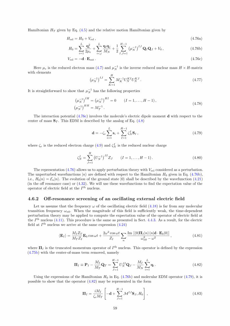
Hamiltonian HT given by Eq. (4.5) and the relative motion Hamiltonian given by

Hrel = H0 + Vrel , (4.76a)

H0 =

L∑i=1

q2i

2µe+

L∑i<j

qiqjMN

+1

2

H−1∑I,J=1

(µ−1N

)IJQIQJ + V0 , (4.76b)

Vrel = −d ·Eext . (4.76c)

Here µe is the reduced electron mass (4.7) and µ−1N is the inverse reduced nuclear mass H ×H-matrix

with elements (µ−1N

)IJ=

H∑K=1

M−1K UKIN UKJN . (4.77)

It is straightforward to show that µ−1N has the following properties(

µ−1N

)IH=(µ−1N

)HI= 0 (I = 1, . . . ,H − 1) ,(

µ−1N

)HH= M−1

T .(4.78)

The interaction potential (4.76c) involves the molecule’s electric dipole moment d with respect to thecenter of mass ST . This EDM is described by the analog of Eq. (4.8)

d = −ζeL∑i=1

si +

H−1∑I=1

ζINSI , (4.79)

where ζe is the reduced electron charge (4.9) and ζIN is the reduced nuclear charge

ζIN =

H∑J=1

(U−1N

)JIZJ (I = 1, . . . ,H − 1) . (4.80)

The representation (4.76) allows us to apply perturbation theory with Vrel considered as a perturbation.The unperturbed wavefunctions |n〉 are defined with respect to the Hamiltonian H0 given in Eq. (4.76b),i.e., H0|n〉 = En|n〉. The evolution of the ground state |0〉 shall be described by the wavefunction (4.21)(in the off resonance case) or (4.32). We will use these wavefunctions to find the expectation value of theoperator of electric field at the Ith nucleus.

4.6.2 Off-resonance screening of an oscillating external electric field

Let us assume that the frequency ω of the oscillating electric field (4.18) is far from any moleculartransition frequency ωn0. When the magnitude of this field is sufficiently weak, the time-dependentperturbation theory may be applied to compute the expectation value of the operator of electric field atthe Ith nucleus (4.11). This procedure is the same as presented in Sect. 4.4.3. As a result, for the electricfield at Ith nucleus we arrive at the same expression (4.24)

〈EI〉 =MIZTMTZI

E0 cosωt+2ω2 cosωt

ZI

∑n

Im [〈0|ΠI |n〉〈n|d ·E0|0〉]ω2n0 − ω2

, (4.81)

where ΠI is the truncated momentum operator of Ith nucleus. This operator is defined by the expression(4.75b) with the center-of-mass term removed, namely

ΠI ≡ PI −MI

MTQT =

H−1∑J=1

UJIN QJ −MI

MN

L∑i=1

qi . (4.82)

Using the expressions of the Hamiltonian H0 in Eq. (4.76b) and molecular EDM operator (4.79), it ispossible to show that the operator (4.82) may be represented in the form

ΠI =iMI

ζeMT

[−d +

H−1∑J=1

MIJSJ , H0

], (4.83)

59

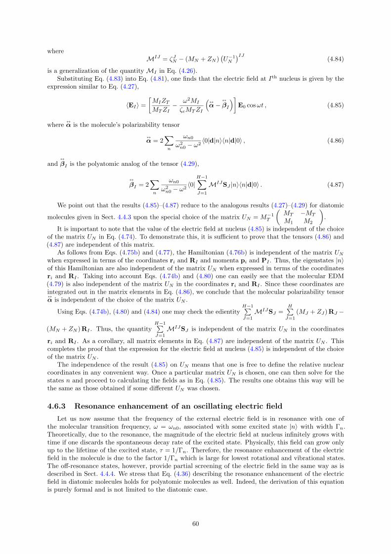
whereMIJ = ζJN − (MN + ZN )

(U−1N

)IJ(4.84)

is a generalization of the quantity MI in Eq. (4.26).Substituting Eq. (4.83) into Eq. (4.81), one finds that the electric field at Ith nucleus is given by the

expression similar to Eq. (4.27),

〈EI〉 =

[MIZTMTZI

− ω2MI

ζeMTZI

(↔α−

↔

βI

)]E0 cosωt , (4.85)

where↔α is the molecule’s polarizability tensor

↔α = 2

∑n

ωn0

ω2n0 − ω2

〈0|d|n〉〈n|d|0〉 , (4.86)

and↔

βI is the polyatomic analog of the tensor (4.29),

↔

βI = 2∑n

ωn0

ω2n0 − ω2

〈0|H−1∑J=1

MIJSJ |n〉〈n|d|0〉 . (4.87)

We point out that the results (4.85)–(4.87) reduce to the analogous results (4.27)–(4.29) for diatomic

molecules given in Sect. 4.4.3 upon the special choice of the matrix UN = M−1T

(MT −MT

M1 M2

).

It is important to note that the value of the electric field at nucleus (4.85) is independent of the choiceof the matrix UN in Eq. (4.74). To demonstrate this, it is sufficient to prove that the tensors (4.86) and(4.87) are independent of this matrix.

As follows from Eqs. (4.75b) and (4.77), the Hamiltonian (4.76b) is independent of the matrix UNwhen expressed in terms of the coordinates ri and RI and momenta pi and PI . Thus, the eigenstates |n〉of this Hamiltonian are also independent of the matrix UN when expressed in terms of the coordinatesri and RI . Taking into account Eqs. (4.74b) and (4.80) one can easily see that the molecular EDM(4.79) is also independent of the matrix UN in the coordinates ri and RI . Since these coordinates areintegrated out in the matrix elements in Eq. (4.86), we conclude that the molecular polarizability tensor↔α is independent of the choice of the matrix UN .

Using Eqs. (4.74b), (4.80) and (4.84) one may check the edientityH−1∑J=1

MIJSJ =H∑J=1

(MJ + ZJ) RJ −

(MN + ZN ) RI . Thus, the quantityH−1∑J=1

MIJSJ is independent of the matrix UN in the coordinates

ri and RI . As a corollary, all matrix elements in Eq. (4.87) are independent of the matrix UN . Thiscompletes the proof that the expression for the electric field at nucleus (4.85) is independent of the choiceof the matrix UN .

The independence of the result (4.85) on UN means that one is free to define the relative nuclearcoordinates in any convenient way. Once a particular matrix UN is chosen, one can then solve for thestates n and proceed to calculating the fields as in Eq. (4.85). The results one obtains this way will bethe same as those obtained if some different UN was chosen.

4.6.3 Resonance enhancement of an oscillating electric field

Let us now assume that the frequency of the external electric field is in resonance with one ofthe molecular transition frequency, ω = ωn0, associated with some excited state |n〉 with width Γn.Theoretically, due to the resonance, the magnitude of the electric field at nucleus infinitely grows withtime if one discards the spontaneous decay rate of the excited state. Physically, this field can grow onlyup to the lifetime of the excited state, τ = 1/Γn. Therefore, the resonance enhancement of the electricfield in the molecule is due to the factor 1/Γn which is large for lowest rotational and vibrational states.The off-resonance states, however, provide partial screening of the electric field in the same way as isdescribed in Sect. 4.4.4. We stress that Eq. (4.36) describing the resonance enhancement of the electricfield in diatomic molecules holds for polyatomic molecules as well. Indeed, the derivation of this equationis purely formal and is not limited to the diatomic case.

60

Since the lowest ro-vibrational states in molecules possess very large lifetime, the resonance enhance-ment due to the factor 1/Γn becomes significantly larger than the screening due to the off-resonancestates. In this case, the electric field is described by the analog of Eq. (4.37)

〈EI〉 ≈ω2meMI

ζee2ZIMTΓn

↔γIE0 sinωt , (4.88)

where the tensor↔γI reads now

↔γI = 2〈0|d|n〉〈n|d|0〉 − 2〈0|

H−1∑J=1

MIJSJ |n〉〈n|d|0〉 . (4.89)

Here MIJ is given in Eq. (4.84).We point out that the expression (4.88) for the enhancement of the electric field at nucleus is valid for

a weak external field since it is obtained in perturbation theory. The condition of the applicability ofperturbation theory reads Ω Γn, where Ω = |〈0|d ·E0|n〉| is the Rabi frequency. For a stronger electricfield one is to apply a more general formula derived non-perturbatively in [13]:

〈EI〉 =ω2meMI

ζee2ZIMT

ΓnΓ2n + 2Ω2

↔γIE0 sinωt . (4.90)

This formula has the same form as in the case of diatomic molecules (4.40) except for the tensor↔γI

given by Eq. (4.89). As a result, the formulae for the critical field Ecrit and the maximal field EmaxI are

the same as given in Eqs. (4.41) and (4.42) but with↔γI given by Eq. (4.89).

4.7 Summary and discussion

In this paper, we derived the general formulae for the screening (4.30) and resonance enhancement(4.40) of an oscillating electric field at a nucleus in a diatomic molecule.

The screening formula (4.30) applies when the frequency of external electric field is far from anytransition frequency in the molecule. This formula may be considered, on the one hand, as a generalizationof the screening of a static electric field in molecules [14] and, on the other hand, as an extension of thescreening formula of oscillating electric field in atoms [11]. For molecules, the screening of electric fieldexhibits some important features. Similarly to the atomic case [11], Eq. (4.30) contains the term with

dynamical polarizability↔α. However, there are extra terms (described by the tensor

↔

β) in Eq. (4.30),which have no analogs in the atomic case.

To uncover the role of the new terms in Eq. (4.30), we considered the examples of some diatomicmolecules in the electric field in different frequency regimes. We found that when the frequency of the

electric field is of order of the frequency of ro-vibrational transitions in a molecule, the↔

β-tensor in Eq.(4.30) gives dominant contribution to the resulting electric field at nucleus since it is enhanced by theratio MI/me. This parameter makes the screening of the low-frequency electric field in molecules verydifferent from that in atoms.

When the frequency of the external field approaches the energies of electronic transitions, the

contributions from both tensors↔α and

↔

β become significant. Thus, the molecules exhibit differentscreening behaviour in different frequency ranges. The typical dependence on the frequency of differentcontributions to the suppression coefficient is presented at Fig. 4.1. In particular, the screening of thefield in molecules in the microwave regime appears not as strong as it is in atoms [11]. The summary ofsuppression coefficients σI for some molecules in various frequency regimes is given in Table 4.1.

When the frequency of the external electric field approaches one of the transition frequency, theresonant excited state in the molecule is responsible for the linear-in-time growth of the electric field atnucleus up to the life-time of the excited state. The off-resonant states, however, provide partial screeningof this electric field as is shown in Eq. (4.36). The resonance enhancement may be up to the factor 109

due to a small width of the state Γ, so it becomes dominating over the suppression factors as in Eq. (4.37).The advantage molecules have over atoms is that they possess ro-vibrational states with energies

in the microwave or even radio-frequency region. These states in molecules typically have very narrowspectral lines that makes the resonance enhancement of the oscillating electric field at nucleus very large.

However, we caution the readers against using the resonance enhancement formula (4.37) for theelectric field at nucleus: Since this result is derived within the perturbatie approach, it is applicable only

61

for sufficiently weak electric field under the constraint (4.39). For a stronger electric field, one shouldapply the non-perturbative formula (4.40) which was derived in [13]. Physically, this formula tells us thateven in the resonance one cannot produce the electric field at nucleus stronger than the Coulomb fieldinside the molecule. The point of the perturbative formula (4.36) is that one can take a very weak electricfield in resonance with the molecular transition to produce sufficiently large oscillating electric field atnucleus. Some particular examples of such weak fields and their amplification factors εI are presented inTable 4.2.

Although our main results (4.30) and (4.40) are derived for the case of diatomic molecules, we presenta generalization of these formulae to the polyatomic molecules in Sect. 4.6.

The results of this paper may have various physical applications since they represent a way out fromthe shielding of a static electric field at nucleus due to the Schiff theorem [4]. In particular, it wouldbe interesting to develop a technique for measuring nuclear EDM using an oscillating electric field inresonance with molecular transition. Many diatomic molecules possess Ω-doubling of states with splittingof order of 100 MHz. Such molecules have already proved useful for measuring electron’s EDM, see, e.g.,[24–26]. One can apply the electric field in resonance with this transition to induce a large electric fieldat nucleus which may be used to measure nuclear EDM. Another use of the results of this paper may berelated to application of laser beams to stimulate nuclear transitions such as the neutron capture in the139La nucleus proposed in [27–29]. These issues deserve separate studies.

Acknowledgments

This work is supported by the Australian Research Council Grant No. DP150101405 and by aGutenberg Fellowship.

Bibliography

[1] T. Chupp, P. Fierlinger, M. Ramsey-Musolf, and J. Singh, arXiv:1710.02504 (2017).

[2] N. Yamanaka, B. K. Sahoo, N. Yoshinaga, T. Sato, K. Asahi, and B. P. Das, Eur. Phys. J. A53, 54(2017).

[3] M. S. Safronova, D. Budker, D. DeMille, D. F. J. Kimball, A. Derevianko, and C. W. Clark, Rev.Mod. Phys. 90, 025008 (2018).

[4] L. I. Schiff, Phys. Rev. 132, 2194 (1963).

[5] P. G. H. Sandars, Phys. Rev. Lett. 19, 1396 (1967).

[6] E. A. Hinds and P. G. H. Sandars, Phys. Rev. A 21, 471 (1980).

[7] O. P. Sushkov, V. V. Flambaum, and I. B. Khriplovich, Zh. Exp. Teor. Fiz. 87, 1521 (1984).

[8] V. Flambaum, I. Khriplovich, and O. Sushkov, Phys. Lett. B 162, 213 (1985).

[9] V. Flambaum, I. Khriplovich, and O. Sushkov, Nuclear Physics A 449, 750 (1986).

[10] V. Dzuba, V. Flambaum, P. Silvestrov, and O. Sushkov, Phys. Lett. A 118, 177 (1986).

[11] V. V. Flambaum, Phys. Rev. A 98, 043408 (2018).

[12] V. A. Dzuba, J. C. Berengut, J. S. M. Ginges, and V. V. Flambaum, Phys. Rev. A 98, 043411 (2018).

[13] V. V. Flambaum and I. B. Samsonov, Phys. Rev. A98, 053437 (2018).

[14] V. V. Flambaum and A. Kozlov, Phys. Rev. A 85, 022505 (2012).

[15] M. Brieger, Chem. Phys. 89, 275 (1984).

[16] M. Mizushima et al., Theory of rotating diatomic molecules (Wiley, 1975).

[17] A. R. Edmonds, Angular momentum in quantum mechanics (Princeton university press, 2016).

[18] F. Grimaldi, A. Lecourt, and C. Moser, Symp. Faraday Soc. 2, 59 (1968).

62

[19] K. A. Peterson and R. C. Woods, J. Chem. Phys. 87, 4409 (1987).

[20] W. Childs, G. Goodman, and L. Goodman, J. Mol. Spectrosc. 115, 215 (1986).

[21] NIST chemistry WebBook, SRD 69 (2018).

[22] E. V. Akindinova, V. E. Chernov, I. Y. Kretinin, and B. A. Zon, Phys. Rev. A 81, 042517 (2010).

[23] B. Sutcliffe (Wiley-Blackwell, 2007), pp. 1–121, ISBN 9780470141731.

[24] J. Baron et al. (ACME), Science 343, 269 (2014).

[25] S. Eckel, P. Hamilton, E. Kirilov, H. W. Smith, and D. DeMille, Phys. Rev. A 87, 052130 (2013).

[26] S. Bickman, P. Hamilton, Y. Jiang, and D. DeMille, Phys. Rev. A 80, 023418 (2009).

[27] D. Zaretskii and V. Lomonosov, Pis’ma Zh. Eksp. Teor. Fiz. 30, 541 (1979).

[28] D. Zaretskii and V. Lomonosov, Zh. Eksp. Teor. Fiz. 81, 429 (1981).

[29] A. Y. Dzyublik, Zh. Eksp. Teor. Fiz. 102, 120 (1992).

63

Chapter 5

Oscillating nuclear electric dipolemoment induced by axion darkmatter produces atomic andmolecular EDMs and nuclear spinrotation

5.1 Overview

Schiff’s theorem states that a static nuclear EDM does not induce atomic or molecular EDM. In thischapter, I demonstrate that an oscillating nuclear EDM does produce measurable atomic and molecularEDMs. Moreover, if one applies an oscillating electric field whose frequency matches that of the oscillatingnuclear EDM then nuclear spin precession happens. By manipulating the atomic or molecular spectrum sothat a level is on resonance with both the field and the nuclear EDM, the effect may be further enhanced.The nuclear spin precession may reach 10−6 radian per second. In terms of energy, this is about fiveorders of magnitude larger than the energy typically measured in the 199Hg experiment.

These results are published in the following paper:

1. V. V. Flambaum and H. B. Tran Tan, Oscillating nuclear electric dipole moment inducedby axion dark matter produces atomic and molecular EDM, Phys. Rev. D 100, 111301(R)(2019), DOI: 10.1103/PhysRevD.100.111301, arXiv:1904.07609,

which I presented at one international conference, one international workshop and one nationalcompetition:

1. Searching for Axions and Axionic Dark Matter with Interference and Axion-inducedNuclear Moments, TeV Particle Astrophysics Conference, University of Sydney, Sydney, Australia,December 2019,

2. Screening and Enhancement of Nuclear Electric Dipole Moments Induced by AxionicDark Matter, Frontiers in Quantum Matter Workshop: Electric Dipole Moments, AustralianNational University, Canberra, Australia, November 2019,

3. Effects of Dark Matter in atomic and molecular phenomena, Australian Institute of PhysicsPostgraduate Presentation Competition, University of Technology Sydney, Sydney, Australia,October 2019.

5.2 Abstract

According to the Schiff theorem, a static nuclear electric dipole moment (EDM) does not produceatomic and molecular EDMs. However, interaction with the axion dark matter field generates nuclear

64

EDMs dN = d0N cos(ωt) which oscillate with the frequency ω = mac

2/~. These oscillating nuclear EDMsgenerate atomic and molecular EDMs proportional to ω2. The resulting atomic and molecular EDMs donot, however, lead to nuclear spin rotation in constant external electric fields. On the other hand, anoscillating electric field penetrates atoms and molecules and can interact with nuclear EDMs. Moreover,if the nuclear EDM oscillation frequency is in resonance with the external field, nuclear spin rotationhappens, with the rotation angle growing linearly with time.

5.3 Introduction

It was suggested in Ref. [1] that interaction with the axionic dark matter produces oscillating neutronand thus oscillating nuclear electric dipole moments (EDMs). We show that such oscillating EDMs will notbe limited by the Schiff theorem [2] and will produce oscillating atomic and molecular EDMs calculatedbelow. However, a constant electric field does not penetrate to the nucleus so there is no interaction withthe nuclear EDM, i.e., there will be no nuclear spin rotation for both static and oscillating nuclear EDMs.

Observable atomic and molecular EDMs are actually produced by the nuclear Schiff moment which issuppressed compared to EDM by an additional second power of the nuclear radius which is very smallon the atomic scale [3–7] (see also [8–14] for other effects producing atomic and molecular EDM). Theeffects produced by the axion-induced Schiff moment have been considered in Ref. [15]. A correspondingexperiment in solids has been proposed in Ref. [16]. The first results of the oscillating neutron EDMand Hg atom’s EDM measurements are presented in Ref. [17] where the limits on the low-mass axioninteraction constant with matter have been improved up to three orders of magnitude.

In this paper, we consider the situation when both the nuclear EDM and the external field areoscillating. In such cases, the external field penetrates to the atomic and molecular nucleus [18–20]and can interact with the nuclear EDM. We demonstrate that in the case where the frequency of theexternal field matches the frequency of the nuclear EDM oscillation, nuclear spin rotation happens withthe rotation angle growing linearly with time. This effect is, in principle, observable.

We will also present the result for the atomic and molecular EDMs induced by nuclear EDMs. It willbe observed that the molecular EDM is larger than its atomic counterpart, due to the fact that nucleimove much slower than electrons so their screening effect is much weaker. As a result, the residual, partlyscreened EDMs in molecules are MN/me times larger than those in atoms. Here MN is the nuclear massand me is the electron mass. Additional MN/me appears due to the small energy intervals betweenrotational states in molecule.

5.4 Screening theorem for time-dependent electric fields andEDMs

As known, a nucleus in a neutral system (atom or molecule) is completely screened from a constantelectric field [2]. We will here present a derivation of this fact following the Appendix in Ref. [21]. Fordefiniteness, we assume that the system in question is a neutral atom in a static homogeneous externalelectric field of an arbitrary strength (we ignore the possibility of atomic ionization and effects of magneticfields).

The Hamiltonian of an atom placed in a static homogeneous external electric field E0 is

H =∑i

[Ki − eφ0 (ri) + eri ·E0] +∑i>j

e2

|ri − rj |− d ·E0, (5.1)

where Ki and ri are the kinetic energy and coordinates of the electrons, d is the static nuclear EDM andφ0 (ri) is the electrostatic nuclear potential given by

φ0 (ri) = e

∫ρ (r) d3r

|ri − r|, (5.2)

where ρ is the nuclear charge distribution. We consider here the case of an infinitely heavy nucleus. Thenuclear recoil correction is not enough to generate an atomic EDM [2].

We add to H an auxiliary term

V = d ·E0 −1

Ze

∑i

d · ∇iφ0 (ri) , (5.3)

65

which, in the linear approximation in d, does not produce any energy shift, 〈V 〉 = 0. Indeed, we have

i

m

[∑i

pi, H

]= −e

∑i

∇iφ0 (ri) + ZeE0, (5.4)

where we have taken into account the fact that the total electron momentum∑i pi commutes with the

electron-electron interaction term. Using Eq. (5.3) and the fact that

i

m〈ψ|

[∑i

pi, H

]|ψ〉 ∝ (Eψ − Eψ) = 0 (5.5)

(ψ is the wavefunction of the Hamiltonian H), we obtain

〈V 〉 =

⟨d ·E0 −

1

Ze

∑i

d · ∇iφ0 (ri)

⟩= 0. (5.6)

To find an EDM one needs to measure a linear energy shift in an external electric field. Since V doesnot contribute to this shift we can add it to the Hamiltonian

H ≡ H + V =∑i

[Ki − eφ (ri) + eri ·E0] +∑i>j

e2

|ri − rj |, (5.7)

where

φ (ri) = φ0 (ri) +1

Zed · ∇iφ0 (ri) . (5.8)

Note that the Hamiltonian H does not contain the direct interaction d ·E0 between the nuclear EDMand external field (Schiff theorem). The dipole term is also canceled out in the multipole expansion ofφ (ri).

Let us now consider the case where the nuclear EDM is time-dependent d = d (t). In this case, Eq.(5.5) becomes

i

m

⟨[∑i

pi, H

]⟩= − 1

m

d

dt

⟨∑i

pi

⟩=

1

m

d 〈pnuc〉dt

∝ d . (5.9)

Therefore, the contribution due to 〈V 〉 is zero in the first order in d. As a result, just as in the caseof a static nuclear EDM, there is no direct interaction between a time-dependent nuclear EDM and astatic external electric field, hence, no nuclear spin rotation. Indeed, the external electric field does notpenetrate to the nucleus (since an atom and its nucleus are not accelerated by a static homogeneouselectric field), so the nuclear EDM has nothing to interact with.

Now consider the case of a time-dependent electric field. In this case, we have

1

m

d 〈pnuc〉dt

∝ E0 , (5.10)

since the external field now penetrates to the nucleus [18–20]. Indeed, the external electric field forcesthe electron shells to oscillate and since the atom’s center of mass stays at rest, the nucleus must move,so the electric field on it is not zero. Therefore, the nuclear EDM interacts with this electric field andnuclear spin rotation happens.

Note that the absence of nuclear spin rotation in the case of a static electric field does not mean thatthe oscillating nuclear EDM does not produce any effect. An oscillating nuclear EDM excites the electronsand produces atomic and molecular EDMs (as demonstrated below). This effect is particularly clear inthe case where the nuclear EDM’s frequency of oscillation is in resonance with some atomic or molecularfrequency, in which case the electronic wavefunciton is a linear combination of two states of oppositeparities and thus gives rise to oscillating atomic and molecular EDMs. Oscilalting nuclear EDMs mayalso be detected using the atomic and molecular transitions they induced, as investigated in Refs. [22–24].

The case where both the nuclear EDM and the external electric field are time-dependent, particularlywhen they are oscillating, is of special interest. As demonstrated in Refs. [18–20], an external electric fieldwhich oscillates with a frequency Ω, E0 ∼ cos Ωt, induces an electric field on the nucleus which oscillateswith the same frequency. The interaction of this field with a nuclear EDM which itself oscillates witha frequency ω, dN ∼ cosωt, is proportional to cosωt cos Ωt. If ω = Ω then this interaction contains atime-independent component and the nuclear spin rotation angle grows linearly with time (see below).

66

5.5 Nuclear EDMs produced by the axion dark matter field

It has been noted in Ref. [25] that the neutron EDM may be produced by the QCD θ term. Numerousreferences and recent results for the neutron and proton EDMs are summarised in Ref. [26]:

dn = −(2.7± 1.2)× 10−16θ e cm ,

dp = (2.1± 1.2)× 10−16θ e cm .(5.11)

Calculations of the nuclear EDM produced by the P,T-odd nuclear forces have been performed in theRefs. [5–7, 27]. For a general estimate of the nuclear EDM it is convenient to use a single-valence-nucleonformula from Ref. [5] and express the result in terms of θ following Ref. [28]:

d ≈ e(q − Z

A

)(1− 2q) ξ 〈σ〉 , (5.12)

where ξ = 7× 10−16θcm.Here q = 1 for the valence proton, q = 0 for the valence neutron, the nuclear spin matrix element

〈σ〉 = 1 if I = l + 1/2 and 〈σ〉 = −I/ (I + 1) if I = l − 1/2. Here, I and l are the total and orbitalmomenta of the valence nucleon.

It was noted in Ref. [1] that the axion dark matter field may be an oscillating θ term and thusgenerates the oscillating neutron EDM. To reproduce the density of dark matter, following Ref. [15], wemay substitute θ(t) = θ0 cos(ωt) where θ0 = 4× 10−18, ω = mac

2/~ and ma is the axion mass.

5.6 Evolution of an osclillating nuclear EDM in an oscillatingelectric field

In this section, we investigate the behavior of an oscillating nuclear EDM dN cosωt when an oscillatingexternal electric field E0 cos Ωt is applied to an atom. It was shown in Refs. [18–20] that the field E0 cos Ωtinduces on the nucleus an electric field of frequency Ω and amplitude

Eoff−resN = −Ω2meα (Ω)

Ze2~2E0 , (5.13)

where α is the atomic polarizabiliy.This result applies in the case where Ω is far away from any atomic transition frequency. In the

case where Ω matches the transition frequency ωn0 from the ground state |0〉 to some state |n〉, EN isresonantly enhanced

Eon−resN = − 2me

~e2Z

Ω2

Γ|〈0|Dz |n〉|2 E0 , (5.14)

where Γ is the width of the state |n〉 and Dz is the atom’s electric dipole operator. Typically, Γ ωn0 = Ωso Eoff−res

N Eon−resN .

In any case, the interaction of the nuclear EDM dN cosωt with the field EN cos Ωt may be written as

V = −dN ·EN cos Ωt cosωt = −dN ·EN

2cos (Ω + ω) t− dN ·EN

2cos (Ω− ω) t . (5.15)

The evolution of the nuclear spin I under the influence of this interaction (without magnetic fields) is

〈I〉 = 〈I〉0 + dN Im 〈I [I ·EN ]〉0sin (Ω + ω) t

Ω + ω+ dN Im 〈I [I ·EN ]〉0

sin (Ω− ω) t

Ω− ω, (5.16)

where 〈.〉0 means the expectation value with respect to the original state of the nuclear spin.If Ω, ω 6= 0 then the second term in Eq. (5.16) is sinusoidal and thus averages to zero. However, in the

case where ω = Ω, the third term in Eq. (5.16) is proportional to t.If we assume that the nucleus carries spin 1/2, which initially points in the x-direction and that

E0 = E0z then in the case where Ω = ω, Eq. (5.16) reads (neglecting the oscillating term)

〈I〉 =1

2x− 1

4dNEN ty , (5.17)

67

which shows that I starts to rotate in the xy-plane and the rotation angle is θ ∼ dNEN t/2. In fact, sincethe result (5.16) was obtained using perturbation theory, it only holds, in the case where Ω = ω, if t issmall. For large t, we should write (neglecting the oscillating term)

〈I〉 =1

2cos

dNEN t

2x− 1

2sin

dNEN t

2y . (5.18)

Note that EN in Eq. (5.18) may take the off-resonance value (5.13) or the resonance value (5.14). Thelatter is of particular interest since in that case EN is enhanced by several orders of magnitude. Thissituation requires Ω = ω = ωn0. When such ‘double resonance’ condition is met, nuclear spin rotationmay be much more significant.

Note that although the analysis of this section was performed for an atom, the same conclusion holdsif a molecule was considered. In fact, molecules have several advantages over atoms. In molecules, nucleialso participate in the screening of an external electric field and since nuclei move much slower thanelectrons, their screening effect of an oscillating electric field is weaken. As a result, the induced fieldon a molecular nucleus is enhanced by a factor of MN/me . 105 in comparison with the field on anatomic nucleus. A further enhancement to the field on a molecular nucleus comes from the small energyintervals between rotational levels in molecules which appear in the denominator [20]. Finally, sincemolecules have rich spectra with small energy intervals which are in the expected range of axion mass,the ‘double resonance’ condition may be more easily satisfied in molecules than in atoms. Achieving thisentails tuning the energy interval between the states |0〉 and |n〉 (using Stark and Zeeman shifts) and thefrequency of the external electric field to match the nuclear EDM oscillation frequency.

5.7 Oscillating atomic EDMs induced by oscillating nuclear EDMs

As remarked earlier, an oscillating nuclear EDM dN cosωt induces oscillating atomic EDMs. In thissection, we provide the calculation for the atomic EDM induced by a nuclear EDM.

The Hamiltonian of an atom in the field of an oscillating nuclear EDM d = d0 cos(ωt) may be writtenas

V = e

Ne∑k=1

d · rkr3k

=i

Ze~[P · d, H0] , (5.19)

where H0 is the Schrodinger or the Dirac Hamiltonian for the atomic electrons in the absence of d,Ne is the number of electrons, Ze is the nuclear charge, Zi = Z − Ne, −e is the electron charge,rk is the electron position relative to the nucleus, P =

∑Nek=1 pk is the total momentum of all atomic

electrons (which commutes with the electron-electron interaction but not with the nuclear-elect interaction

U = −∑Nek=1 Ze

2/rk: [P, H0] = [P, U ] = −i~Ze2∑Nek=1∇

1rk

). Here we assumed that the nuclear mass isinfinite and neglect very small effects of the Breit and magnetic interactions.

Using H0 |n〉 = En |n〉 we obtain the matrix element of V between atomic states |n〉 and |m〉

〈n|V |m〉 =iEnmZe~

〈n|P · d |m〉 , (5.20)

where Enm = En − Em.Using the time dependent perturbation theory [29] for the oscillating perturbation V = V0 cosωt and

Eq. (5.20) we obtain a formula for the induced atomic EDM

Dind = 2∑n

E0nRe (〈0|V |n〉 〈n|D |0〉)E2

0n − ε2=

2

Ze~∑n

E20nIm (〈0|P · d |n〉 〈n|D |0〉)

E20n − ε2

, (5.21)

where ε = ~ω and D = −e∑Nek=1 rk.

The energy dependent factor may be presented as

E20n

E20n − ε2

= 1 +ε2

E20n − ε2

. (5.22)

The energy independent term 1 on the right hand side allows us to sum over states |n〉 in Eq. (5.21).Using the closure condition and the commutator relation [P,D] = −ie~Ne, this term gives

Datom = d + Dind =ZiZ

d +2

Ze~∑n

ε2Im (〈0|P · d |n〉 〈n|D |0〉)E2

0n − ε2. (5.23)

68

We observe that, in agreement with the Schiff theorem, the atomic electric dipole moment Datom

vanishes in a neutral atom (Zi = Z −Ne = 0) with static nuclear EDM (ε = ~ω = 0).Assume that nuclear EDM d is directed along the z-axis. Using the non-relativistic commutator

relation P = − imee~ [H0,D] (where me is the electron mass), we can express the atomic EDM in terms ofthe atomic dynamical polarisability αzz(ω)

Dzatom =

dzZ

(Zi −

meε2αzz

e2~2

), αzz = 2

∑n

En0 |〈0|Dz |n〉|2

E2n0 − ε2

. (5.24)

The axion field oscillation frequency may be very small on the atomic scale, therefore, we may usestatic polarisabilities in this expression which are known for all atoms. The formula (5.24) may berewritten, with the energy and the polarizabilty expressed in atomic units ε = ε

e2/aBand αzz = αzz

a3B(where aB is the Bohr radius), as:

Dzatom =

Zi − ε2αzzZ

dz (5.25)

Since the atomic EDM Datom is proportional to 1/Z, it appears that the shielding is stronger inheavy atoms. This, however, is not necessary the case since, for example in hydrogen and helium αzz ∼ 1whereas αzz ∼ 400 in caesium (Z=55). Indeed, the numerical value of the polarizability αzz in atomicunits often exceeds the value of the nuclear charge Z, therefore, the suppression of EDM in a neutralatom mainly comes from the small frequency of the dark matter field oscillations in atomic units, ε.

5.8 Oscillating molecular EDMs induced by oscillating nuclearEDMs

We see from the first line in Eq. (5.24) that the residual EDM in a neutral system (Zi = 0) isproportional to the mass m of the particle which produces the screening of the nuclear EDM d. Masses ofnuclei MN in a molecule are up to 5 orders of magnitude larger than the mass of electron me. In addition,the interval between molecular rotational energy levels (∼ me/MN atomic units) are many orders ofmagnitude smaller than typical energy intervals in atoms and this may give an additional enormousadvantage, see the denominator in the second line in Eq. (5.24). Finally, since the molecular spectra arevery rich, the energy intervals are small and may be tuned by electric and magnetic fields, it is easier tobring them into resonance with the small oscillation frequency of the axion dark matter field.

Calculations presented in the Supplemental Material give the following results for the induced electricdipole of a neutral diatomic molecule when ε is smaller or of the order of the first rotational energy Erot

DEDMmol ≈

2µN XdErot

3e~2

ε2

E2rot − ε2

(d1

Z1− d2

Z2

), (5.26)

where µN = M1M2/ (M1 +M2) is the reduced nuclear mass, X is the ground state inter-nuclear distance,d is the ground state intrinsic electric dipole of a polar molecule and Erot ≈ ~2µ−1

N X−2 is the energy ofthe first rotational state and d1,2 are the nuclear EDMs. In writing Eq. (5.26), we have assumed that themolecular ground state has total angular momentum 0.

For d1 ∼ d2, we see that the lighter nucleus gives dominating contribution. In other words, if Z1 Z2

then the term d2/Z2 drops out. We assume this is the case. In the limits ε Erot and ε Erot, Eq.(5.26) gives

DEDMmol

d1≈

2ε2µ2

N X3d

3e~4Z1ε Erot ,

2d3eZ1X

ε Erot .(5.27)

We see that in the small axion mass limit (ε = mac2 Erot), heavy molecules have an advantage

(µ2N/Z1). In the large axion mass limit (ε = mac

2 Erot), the ratio of the EDMs is independent of εand has asymptotic value 2d/

(3eZ1X

)< 2/ (3Z1) ≤ 2/3 (d ∼ eX for polar molecule) so molecules with

at least one light nucleus are more advantageous.The result (5.26) applies for the off-resonance case. If ε = Erot then we have the following relation

between the oscillation amplitudes of DEDMmol and d1;

DEDMmol ≈

2d

3eZ1X

Erot

Γd1 , (5.28)

69

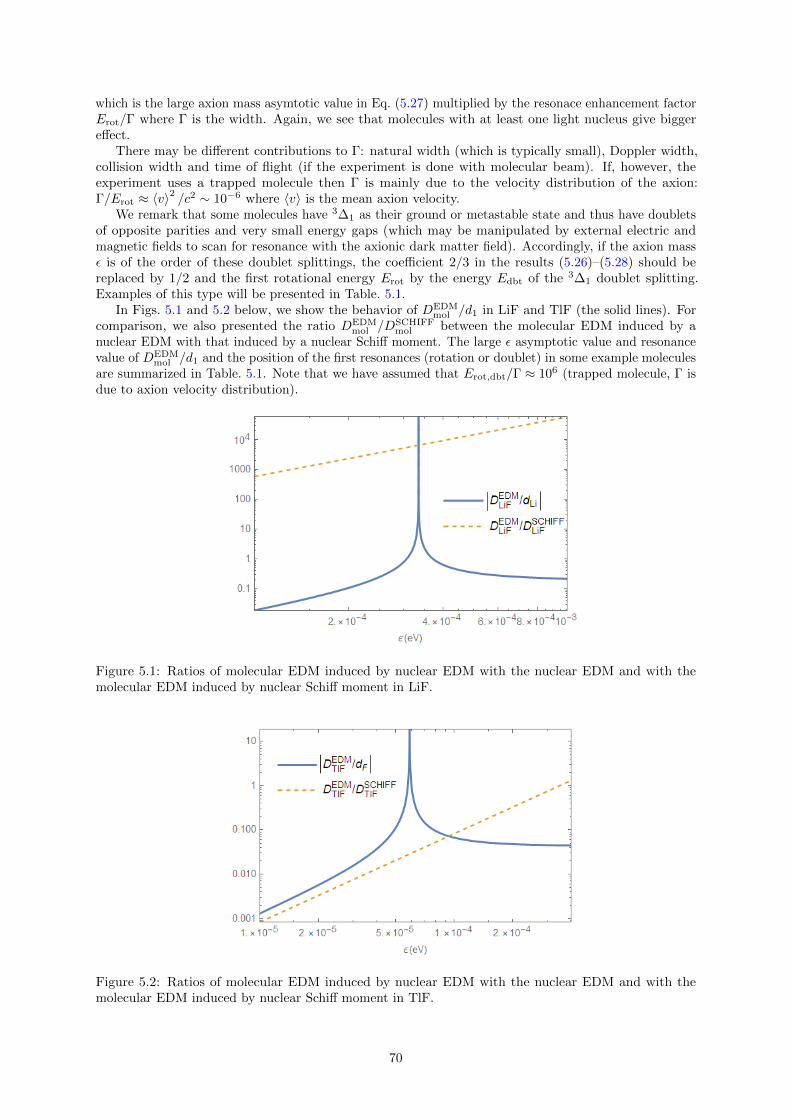
which is the large axion mass asymtotic value in Eq. (5.27) multiplied by the resonace enhancement factorErot/Γ where Γ is the width. Again, we see that molecules with at least one light nucleus give biggereffect.

There may be different contributions to Γ: natural width (which is typically small), Doppler width,collision width and time of flight (if the experiment is done with molecular beam). If, however, theexperiment uses a trapped molecule then Γ is mainly due to the velocity distribution of the axion:Γ/Erot ≈ 〈v〉2 /c2 ∼ 10−6 where 〈v〉 is the mean axion velocity.

We remark that some molecules have 3∆1 as their ground or metastable state and thus have doubletsof opposite parities and very small energy gaps (which may be manipulated by external electric andmagnetic fields to scan for resonance with the axionic dark matter field). Accordingly, if the axion massε is of the order of these doublet splittings, the coefficient 2/3 in the results (5.26)–(5.28) should bereplaced by 1/2 and the first rotational energy Erot by the energy Edbt of the 3∆1 doublet splitting.Examples of this type will be presented in Table. 5.1.

In Figs. 5.1 and 5.2 below, we show the behavior of DEDMmol /d1 in LiF and TlF (the solid lines). For

comparison, we also presented the ratio DEDMmol /DSCHIFF

mol between the molecular EDM induced by anuclear EDM with that induced by a nuclear Schiff moment. The large ε asymptotic value and resonancevalue of DEDM

mol /d1 and the position of the first resonances (rotation or doublet) in some example moleculesare summarized in Table. 5.1. Note that we have assumed that Erot,dbt/Γ ≈ 106 (trapped molecule, Γ isdue to axion velocity distribution).

Figure 5.1: Ratios of molecular EDM induced by nuclear EDM with the nuclear EDM and with themolecular EDM induced by nuclear Schiff moment in LiF.

Figure 5.2: Ratios of molecular EDM induced by nuclear EDM with the nuclear EDM and with themolecular EDM induced by nuclear Schiff moment in TlF.

70

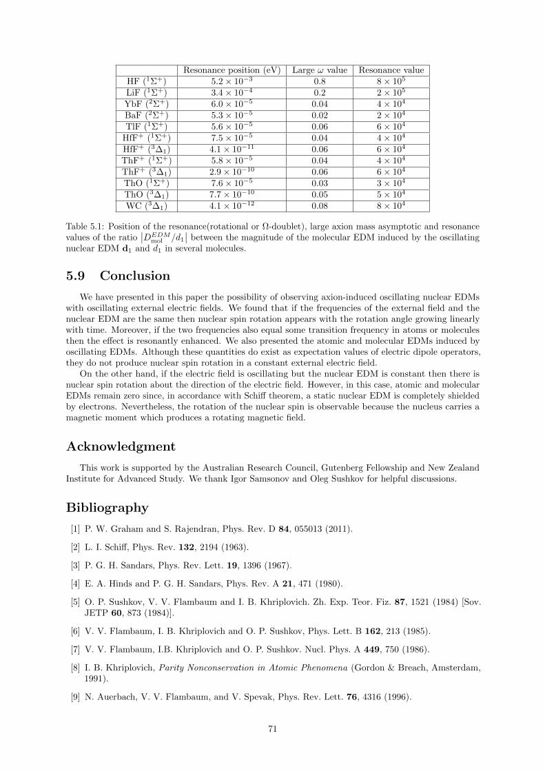
Resonance position (eV) Large ω value Resonance valueHF (1Σ+) 5.2× 10−3 0.8 8× 105

LiF (1Σ+) 3.4× 10−4 0.2 2× 105

YbF (2Σ+) 6.0× 10−5 0.04 4× 104

BaF (2Σ+) 5.3× 10−5 0.02 2× 104

TlF (1Σ+) 5.6× 10−5 0.06 6× 104

HfF+ (1Σ+) 7.5× 10−5 0.04 4× 104

HfF+ (3∆1) 4.1× 10−11 0.06 6× 104

ThF+ (1Σ+) 5.8× 10−5 0.04 4× 104

ThF+ (3∆1) 2.9× 10−10 0.06 6× 104

ThO (1Σ+) 7.6× 10−5 0.03 3× 104

ThO (3∆1) 7.7× 10−10 0.05 5× 104

WC (3∆1) 4.1× 10−12 0.08 8× 104

Table 5.1: Position of the resonance(rotational or Ω-doublet), large axion mass asymptotic and resonancevalues of the ratio

∣∣DEDMmol /d1

∣∣ between the magnitude of the molecular EDM induced by the oscillatingnuclear EDM d1 and d1 in several molecules.

5.9 Conclusion

We have presented in this paper the possibility of observing axion-induced oscillating nuclear EDMswith oscillating external electric fields. We found that if the frequencies of the external field and thenuclear EDM are the same then nuclear spin rotation appears with the rotation angle growing linearlywith time. Moreover, if the two frequencies also equal some transition frequency in atoms or moleculesthen the effect is resonantly enhanced. We also presented the atomic and molecular EDMs induced byoscillating EDMs. Although these quantities do exist as expectation values of electric dipole operators,they do not produce nuclear spin rotation in a constant external electric field.

On the other hand, if the electric field is oscillating but the nuclear EDM is constant then there isnuclear spin rotation about the direction of the electric field. However, in this case, atomic and molecularEDMs remain zero since, in accordance with Schiff theorem, a static nuclear EDM is completely shieldedby electrons. Nevertheless, the rotation of the nuclear spin is observable because the nucleus carries amagnetic moment which produces a rotating magnetic field.

Acknowledgment

This work is supported by the Australian Research Council, Gutenberg Fellowship and New ZealandInstitute for Advanced Study. We thank Igor Samsonov and Oleg Sushkov for helpful discussions.

Bibliography

[1] P. W. Graham and S. Rajendran, Phys. Rev. D 84, 055013 (2011).

[2] L. I. Schiff, Phys. Rev. 132, 2194 (1963).

[3] P. G. H. Sandars, Phys. Rev. Lett. 19, 1396 (1967).

[4] E. A. Hinds and P. G. H. Sandars, Phys. Rev. A 21, 471 (1980).

[5] O. P. Sushkov, V. V. Flambaum and I. B. Khriplovich. Zh. Exp. Teor. Fiz. 87, 1521 (1984) [Sov.JETP 60, 873 (1984)].

[6] V. V. Flambaum, I. B. Khriplovich and O. P. Sushkov, Phys. Lett. B 162, 213 (1985).

[7] V. V. Flambaum, I.B. Khriplovich and O. P. Sushkov. Nucl. Phys. A 449, 750 (1986).

[8] I. B. Khriplovich, Parity Nonconservation in Atomic Phenomena (Gordon & Breach, Amsterdam,1991).

[9] N. Auerbach, V. V. Flambaum, and V. Spevak, Phys. Rev. Lett. 76, 4316 (1996).

71

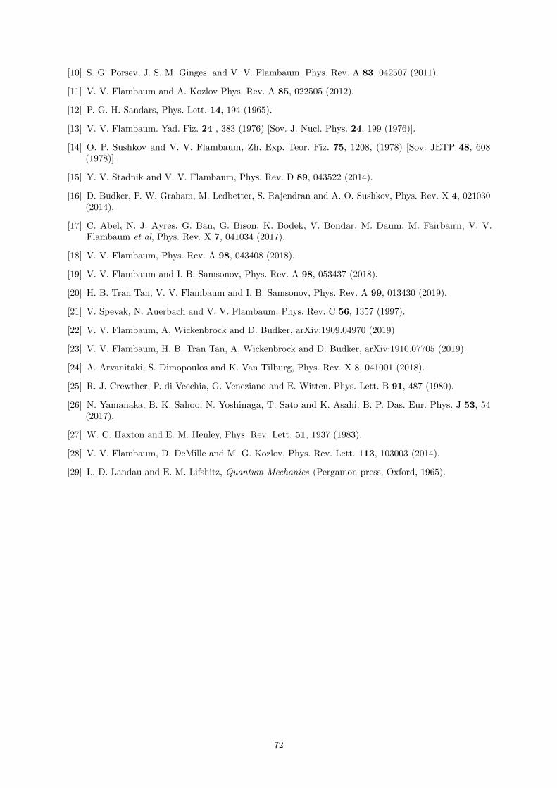
[10] S. G. Porsev, J. S. M. Ginges, and V. V. Flambaum, Phys. Rev. A 83, 042507 (2011).

[11] V. V. Flambaum and A. Kozlov Phys. Rev. A 85, 022505 (2012).

[12] P. G. H. Sandars, Phys. Lett. 14, 194 (1965).

[13] V. V. Flambaum. Yad. Fiz. 24 , 383 (1976) [Sov. J. Nucl. Phys. 24, 199 (1976)].

[14] O. P. Sushkov and V. V. Flambaum, Zh. Exp. Teor. Fiz. 75, 1208, (1978) [Sov. JETP 48, 608(1978)].

[15] Y. V. Stadnik and V. V. Flambaum, Phys. Rev. D 89, 043522 (2014).

[16] D. Budker, P. W. Graham, M. Ledbetter, S. Rajendran and A. O. Sushkov, Phys. Rev. X 4, 021030(2014).

[17] C. Abel, N. J. Ayres, G. Ban, G. Bison, K. Bodek, V. Bondar, M. Daum, M. Fairbairn, V. V.Flambaum et al, Phys. Rev. X 7, 041034 (2017).

[18] V. V. Flambaum, Phys. Rev. A 98, 043408 (2018).

[19] V. V. Flambaum and I. B. Samsonov, Phys. Rev. A 98, 053437 (2018).

[20] H. B. Tran Tan, V. V. Flambaum and I. B. Samsonov, Phys. Rev. A 99, 013430 (2019).

[21] V. Spevak, N. Auerbach and V. V. Flambaum, Phys. Rev. C 56, 1357 (1997).

[22] V. V. Flambaum, A, Wickenbrock and D. Budker, arXiv:1909.04970 (2019)

[23] V. V. Flambaum, H. B. Tran Tan, A, Wickenbrock and D. Budker, arXiv:1910.07705 (2019).

[24] A. Arvanitaki, S. Dimopoulos and K. Van Tilburg, Phys. Rev. X 8, 041001 (2018).

[25] R. J. Crewther, P. di Vecchia, G. Veneziano and E. Witten. Phys. Lett. B 91, 487 (1980).

[26] N. Yamanaka, B. K. Sahoo, N. Yoshinaga, T. Sato and K. Asahi, B. P. Das. Eur. Phys. J 53, 54(2017).

[27] W. C. Haxton and E. M. Henley, Phys. Rev. Lett. 51, 1937 (1983).

[28] V. V. Flambaum, D. DeMille and M. G. Kozlov, Phys. Rev. Lett. 113, 103003 (2014).

[29] L. D. Landau and E. M. Lifshitz, Quantum Mechanics (Pergamon press, Oxford, 1965).

72

Chapter 6

Atomic and molecular transitionsinduced by axions via oscillatingnuclear moments

6.1 Overview

In the presence of a periodic perturbation a quantum mechanical system undergoes transition. Afamiliar example is the atomic and molecular transitions induced by external electromagnetic fields.However, it is worth noting that the perturbation does not have to come from outside to have such aneffect. In this chapter, I consider the transitions induced by various oscillating CP -violating nuclearmoments inside atoms and molecules. These oscillating nuclear moments may be induced by axion DarkMatter. I demonstrate that these transitions are, in principle, observable.

As the result of this research, I have published a paper:

1. V. V. Flambaum, H. B. Tran Tan, D. Budker and A. Wickenbrock, Atomic and moleculartransitions induced by axions via oscillating nuclear moments, Phys. Rev. D 101, 073004(2020), DOI: 10.1103/PhysRevD.101.073004, arXiv:1910.07705,

and presented it at one international conference, one international workshop and one nationalcompetition:

1. Searching for Axions and Axionic Dark Matter with Interference and Axion-inducedNuclear Moments, TeV Particle Astrophysics Conference, University of Sydney, Sydney, Australia,December 2019,

2. Screening and Enhancement of Nuclear Electric Dipole Moments Induced by AxionicDark Matter, Frontiers in Quantum Matter Workshop: Electric Dipole Moments, AustralianNational University, Canberra, Australia, November 2019,

3. Effects of Dark Matter in atomic and molecular phenomena, Australian Institute of PhysicsPostgraduate Presentation Competition, University of Technology Sydney, Sydney, Australia,October 2019.

6.2 Abstract

The interaction of standard model’s particles with the axionic Dark Matter field may generateoscillating nuclear electric dipole moments (EDMs), oscillating nuclear Schiff moments and oscillatingnuclear magnetic quadrupole moments (MQMs) with a frequency corresponding to the axion’s Comptonfrequency. Within an atom or a molecule an oscillating EDM, Schiff moment or MQM can drive transitionsbetween atomic or molecular states. The excitation events can be detected, for example, via subsequentfluorescence or photoionization. Here we calculate the rates of such transitions. If the nucleus has octupoledeformation or quadrupole deformation then the transition rate due to Schiff moment and MQM canbe up to 10−16 transition per molecule per year. In addition, an MQM-induced transition may be of

73

M2-type, which is useful for the elimination of background noise since M2-type transitions are suppressedfor photons.

6.3 Introduction

The nature of dark matter (DM) remains unknown. The axion is a prominent dark matter candidateoriginally introduced in the 1970s to explain the apparent charge-parity (CP) symmetry of the stronginteractions [1–4]. Traditional searches for axion and axion-like particles (ALPs)1 rely on the conversionbetween axion and photon in a strong magnetic field [5, 6]. Helioscope experiments including Sumico[7–11], CAST [12–15], SOLAX [16, 17], COSME [18], CDMS [19–22] and IAXO [23–25] convert solaraxions into photons for detection. Haloscope experiments such as ADMX [26–28], HAYSTAC [29, 30]and ORGAN [31] convert cosmic axions into photons in microwave cavities and detect these photonsresonantly with SQUIDs. Light-shining-through-a-wall (LSW) experiments including ALPS [32–34],OSQAR [35–37] and GammeV [38] convert photons into axions, use a wall to block all the photons butnot the axions, and then convert the axions back into photons for detection behind the wall. Finally,experiments like PVLAS [39–41], Q & A [42] and BMV [43, 44] search for optical birefringence (differencein optical refractive indices for different polarizations) and dichroism (difference in absorption of light ofdifferent polarizations) due to interconversion with axions [45].

Other proposals to search for axion DM include converting axions into magnons in a ferromagnet[46, 47], using dielectric haloscopes with improved sensitivity [48–51], using nuclear magnetic resonanceto search for axion-mediated CP-violating forces [52–55], detecting the oscillating magnetic flux sourcedby the axions entering a static magnetic field [56], using electron spin resonance in magnetized mediato detect the oscillating effective magnetic field induced by axions [57], using superconductors [58]and semiconductors [59], using an LC circuit (Dark Matter radio) [60–62], using Josephson junctions[63, 64], using photon interferometry [65], using axion-induced resonant molecular transitions [66], usinglaser-spectroscopy techniques to probe axion-induced atomic and molecular tranistions [67], looking foran axion-induced topological Casimir effect [68], using a photon field (instead of a magnetic field) totrigger axion-to-photon decay then detecting the product photons with Raman scattering [69] and usingthe interference of axion and photon absorption in atoms and molecules [70].

Recently, a new class of experiments have also been proposed to look for parity- and time-reversal-invariance-violating (P,T-odd) effects due to couplings of axions to Standard Model (SM) particles [71–75].Assuming that the dark matter in the Milky Way consists of axions , the dark matter field can bedescribed as a field oscillating at a frequency close to the Compton frequency of the axion. The interactionof SM particles with this oscillating axion field induces oscillating electric dipole moments (EDMs),oscillating Schiff moments and an oscillating magnetic quadrupole moments (MQMs) of fundamentalparticles, nuclei, atoms, and molecules [71, 74]. These resulting moments then cause the precession ofparticle’s spins due to gradients in the axion field (the axion-wind effect) [76] and may thus, in principle,be detected. The CASPEr experiments [72] search for spin precession due to the oscillating nuclear Schiffmoment, which is related to the nucleon EDMs and axion-induced P,T-odd nuclear forces, and axionwind with nuclear magnetic resonance. First results constraining the axion-nucleon couplings have beenpublished by CASPEr [77, 78], as well as by other experiments re-analyzing existing data obtained in theneutron-EDM [79] and atomic co-magnetometer experiments [80] and trapped anti-proton experiment[81].

In this paper, we analyze the effect of an axion-induced oscillating nuclear EDM, an oscillating nuclearSchiff moment and an oscillating nuclear MQM in atoms and molecules. Such oscillating moments mayinduce transitions in the atom or molecule if the transition frequency matches the axion oscillationfrequency. In fact, nuclear-EDM-induced atomic and molecular transitions were already discussed in Ref.[82]. In this work, we extend the discussion to the case of Schiff-moment-induced- and nuclear-MQM-induced transitions whose rates, as we will demonstrate, may be several orders of magnitude larger thanthat of an EDM-induced transitions.

The rest of the paper is organized as follows. In Sect. 6.4, we provide a brief revision of the nuclearEDM, nuclear Schiff moment, nuclear MQM and how these moments might be produced by an oscillatingaxion DM field. In Sects. 6.5 and 6.6, we estimate the rates of the atomic and molecular transitionsinduced by the oscillating nuclear moments and discuss the scaling of these rates with respect to relevantatomic and molecular parameters. Sect. 7.7 contains a brief summary of our finding and several comments

1ALPs are pseudoscalar particles like the axion that do not, however, solve the strong-CP problem; we refer to bothaxions and ALPs as ‘axions’ in this paper.

74

on the feasibility of experimental observation of the effects.

6.4 Nuclear moments produced by the axion dark matter field

In this section, we give a brief overview of three nuclear moments which give rise to P,T-odd interactionswith the electrons. These are the nuclear EDM, nuclear Schiff moment and the nuclear MQM. The firsttwo moments arise due to P,T-odd-interaction-induced charge distribution inside the nucleus whereas thelast moment arises due to P,T-odd-interaction-induced current distribution inside the nucleus. We willalso explain the connection between an oscillating axion DM field and the oscillating nuclear moments.

6.4.1 Nuclear EDM

The P,T-odd interaction of the atomic electrons with a nuclear EDM d has the familiar form

VEDM = e

Ne∑k=1

d · rkr3k

, (6.1)

where Ne is the number of the electrons, −e is the electron charge and rk is the electron position relativeto the nucleus.

The EDM d of a nucleus arises from the inherent EDMs of the nucleons and from the P,T-oddinteractions between the nucleons. As noted in Ref. [1–4, 83], a neutron EDM may be produced by theso-called ‘QCD θ-term’, where the parameter θ is the axion field strength. Numerous references andrecent results for the neutron and proton EDMs are summarised in the review [84]

dn = −(2.7± 1.2)× 10−16θ e cm ,

dp = (2.1± 1.2)× 10−16θ e cm .(6.2)

Apart from contribution from the neutron and proton EDMs (6.2), the EDM of a nucleus also receivescontributions arising from P,T-odd interactions between nucleons. Calculations of the EDM of a nucleuswith more than one nucleon produced by the P,T-odd nuclear forces were performed in Refs. [85–102].For a general estimate of such a nuclear EDM, it is convenient to use a single-valence-nucleon model inwhich the P,T-odd interaction between the valence nucleon with the nuclear core is given by [86]

HPT =G√

2

η

2mpσ · ∇ρ (r) , (6.3)

where G is the Fermi weak interaction constant, η is a constant which characterizes the strength of theP,T-odd nucleon-nucleon interaction, σ is the nuclear spin operator, ρ (r) is the density of the nuclearcore and mp is the proton mass. The nuclear EDM in this case is that of the valence nucleon, given by

d = e (q − Z/A) 〈r〉 (6.4)

where r is the position operator of the valence nucleon with respect to the nuclear core, q = 1 for thevalence proton and q = 0 for the valence neutron. The effective charge e (q − Z/A) appears due to recoileffect.

Using Eqs. (6.3) and (6.4) and expressing the result in terms of θ following Ref. [103], we obtain thePT-odd force contribution to the nuclear EDM

d ≈ 7× 10−16

(q − Z

A

)(1− 2q) 〈σ〉θ e cm , (6.5)

where the nuclear spin matrix element is 〈σ〉 = 1 if j = l+ 1/2 and 〈σ〉 = −j/ (j + 1) if j = l− 1/2. Here,j and l are the total and orbital momenta of the valence nucleon.

There are many specific results for the 2H and 3He EDMs, see, e.g., reviews [100, 104]. Within theerror bars, the deuterium EDM is consistent with zero due to the cancellation between the proton andneutron contributions. The 3He nucleus contains an unpaired neutron. Using the calculation of theP,T-odd nuclear force contribution from Refs. [97–99] (−1.5× 10−16θ e cm) and the value of the neutronEDM from Eq. (6.2), we obtain for the 3He EDM

d(3He) = (−4.2± 1.5)× 10−16θ e cm , (6.6)

which is close to the estimate obtained using Eq. (9.12d), which gives d(3He) = −4.7× 10−16θ e cm, eventhough the latter does not include the contribution of the neutron EDM.

75

6.4.2 Nuclear Schiff moment

According a theorem by Schiff [105], a static nuclear EDM does not induce an atomic or molecularEDM in a neutral atom or molecule. This reduces to the fact that the P,T-odd interaction between anelectron and the nucleus must have the form [86, 106]

V (R) = −Ze2

[∫ρ (r) d3r

|R− r|+ 〈r〉 · ∇

∫ρ (r) d3r

|R− r|

](6.7)

where R is the electron position operator, ρ (r) is the nuclear charge density normalized to∫ρ (r) d3r = 1

and 〈r〉 = Z∫ρ (r) rd3r.

The dipole term of this interaction reads2 [86]

VSCHIFF = 4πS ·∇ρ (R) , (6.8)

where S is the Schiff moment of the nucleus, defined by

S =e

10

[⟨r2r⟩− 5

3Z

⟨r2⟩〈r〉], (6.9)

where 〈rn〉 = Z∫ρ (r) rnd3r are the moments of the nuclear charge density and r is measured from the

nuclear center of mass (n = 2, 3 is relevant in Eq. (6.9)).For a spherical nucleus with one unpaired nucleon, we can use the model Eq. (6.3), in which Eq. (6.9)

givesS = SI/I ,

S = −7× 10−7θeq

[(〈σ〉+

1

I + 1

)〈r2〉 − 5

3〈σ〉r2

q

],

(6.10)

where I is the nuclear spin, q and 〈σ〉 are defined as in Eq. (9.12d) and r2q is the mean square charge

radius. Approximately, 〈r2〉 ≈ r2q ≈ (3/5)R2 where R = r0A

1/3 is the mean bound-state radius of thenucleus (r0 ≈ 1.5 fm and A is the nuclear mass number).

It is observed from Eq. (6.9) that the Schiff moment is a result of adding two terms of oppositesign. These two terms are often not known with sufficient accuracy so the result of calculating theSchiff moment becomes unreliable. Also, the Schiff moment is determined by the charge distribution ofthe protons. However, it is directed along the nuclear spin which, for example in 199Hg, is carried bythe valence neutron, so the Schiff moment is determined by the many-body effects which are harder tocalculate. The calculation of nuclear EDMs, on the other hand, does not suffer from these problems (suchas the difference of two nearly equal terms) and thus have certain computational advantages.

Despite of these difficulties, numerical calculations of the Schiff moments do exist. Some numericallycomputed values for the Schiff moments of spherical nuclei with one unpaired nucleon are [86–88, 107–111]

S(

205Tl)≈ −0.027θ e fm3 ,

S(

199Hg)≈ −0.005θ e fm3 .

(6.11)

We note in passing that there are experimental limits on the static Schiff moments of 205Tl and 199Hg,e.g.,

∣∣S199Hg

∣∣ . 3.1× 10−13e fm3 corresponding to |θ| . 10−10 [112–114].In nuclei with octupole deformation, the nuclear Schiff moments may be enhanced by 100 to 1000

times (thanks to the small energy differences of nuclear levels with opposite parity and collective effects)[106, 111, 115–118]

S(

153Eu)≈ 3.7 θ e fm3 ,

S(

225Ra)≈ θ e fm3 ,

S(

227Ac)≈ 10 θ e fm3 ,

S(

229Th)≈ 2 θ e fm3 ,

S(

235U)≈ 3 θ e fm3 ,

S(

237Np)≈ 6 θ e fm3 .

(6.12)

2A better form for this interaction which takes into account the finite size of the nucleus is available, see Ref. [107]; forour estimate, the form (6.26) is sufficient.

76

It should also be mentioned that for the Schiff moment of a nucleus with octuple deformation, theaforementioned problem with the cancellation of two nearly equal terms does not arise since the first termin Eq. (6.9) is significantly enhanced whereas the second term is not (it is zero for similar distributionof protons and neutrons) and the result is stable. The calculation of the Schiff moment is, in this case,reduced to that of the expectation value of the P,T-odd interaction over intrinsic states of the deformednucleus.

6.4.3 Nuclear MQM

Since there exists nucleon currents inside a nucleus, apart from electric interaction, the nucleus canalso have magnetic interactions with electrons. The most familiar of such interaction, the magnetic dipoleinteraction, is P,T-even and is thus of no interest to us. The first P,T-odd magnetic interaction is thusbetween the electron and the MQM of the nucleus, given by [86, 119]

VMQM = − M

4I (2I − 1)TijAij , (6.13)

(summation over the indices i, j is implied) where the tensor Tij is defined by (I is again the nuclear spin)

Tij = IiIj + IjIi −2

3δijI (I + 1) , (6.14)

and the tensor Aij by

Aij = εnmiαn∂m∂j1

r. (6.15)

Here, M is the magnitude of the MQM, αn are the Dirac alpha matrices and r the distance from theelectron to the nucleus.

The MQM of a spherical nucleus with one unpaired nucleon is given by [86, 103, 120]

M =[d− 6× 10−16θ (µ− q) (e cm)

]λp (2I − 1) 〈σ〉 , (6.16)

where d is the valence nucleon’s EDM, µ is its magnetic dipole moment in nuclear magnetons, q, σ, I areas defined in Eqs. (9.12d) and (6.9) and λp = ~/mpc = 2.1× 10−14 cm (mp is the proton mass).

Some values for the MQM of spherical nuclei are [86]

M(

131Xe)≈ −3× 10−29θ e cm2 ,

M(

201Hg)≈ 5× 10−29θ e cm2 .

(6.17)

If the nucleus in question has quadrupole deformation, collective effects generally enhance the nuclearMQM by one order of magnitude [103, 120–122]

M(

173Yb)≈ −9× 10−28θ e cm2 ,

M(

177Hf)≈ −1× 10−27θ e cm2 ,

M(

179Hf)≈ −2× 10−27θ e cm2 ,

M(

181Ta)≈ −2× 10−27θ e cm2 ,

M(

229Hf)≈ −1× 10−27θ e cm2 .

(6.18)

6.4.4 Effects of an oscillating axion DM field

Reference [71] discussed the possibility that the dark matter field is, in fact, an oscillating axion fieldwhich generates neutron EDMs. This axion field may also generate oscillating nuclear EDMs, oscillatingnuclear Schiff moments and oscillating nuclear MQMs [74]. In short, the parameter θ, which is theaxion field strength, is now periodic with respect to time instead of being static. Relating the value ofthe axion field to the local dark matter density (Ref. [74]), we may substitute θ(t) = θ0 cos(ωt) whereθ0 = 4 × 10−18, ω = mac

2/~ and ma is the axion mass3. It is important to keep in mind that ALPsinducing larger dipole moments are also among viable DM candidates, so an experiment with sensitivityless than that necessary to detect axionic DM could already be sensitive to DM composed of such ALPs.

3It is worth mentioning that axions are a stochastic field with a finite coherence times τc ≈ 10−6hmac2

, see, for example Ref.

[123]. In this paper, by θ0 we mean√〈θ20〉.

77

6.5 Atomic transitions induced by oscillating nuclear moments

We have presented in the last section the possibility of having oscillating nuclear EDMs, Schiff momentsand MQMs. The interactions of these moments with the atomic electrons may cause electronic transitions.In what follows, we provide estimates of the transition rates due to the interactions with these moments.

6.5.1 Nuclear EDM contribution

The interaction of the atomic electrons with a nuclear EDM (6.1) may also be written as

V EDMatom = e

Ne∑k=1

d · rkr3k

=i

Ze~[P · d, H0] , (6.19)

where H0 is the (Schrodinger or Dirac) Hamiltonian for the atomic electrons in the absence of d and

P =∑Nek=1 pk is the total momentum of all atomic electrons.

The second equal sign in Eq. (6.19) holds because we have assumed that the nuclear mass is infiniteand neglected the small effects of the Breit and magnetic interactions. The operator P commutes with theelectron-electron interaction but does not commute with U , the potential energy due to the interactionwith the nucleus

U = −Ne∑k=1

Ze2/rk , (6.20)

so we have

[P, H0] = [P, U ] = −i~Ze2Ne∑k=1

∇ 1

rk= i~Ze2

Ne∑k=1

rkr3k

. (6.21)

Using the nonrelativistic relation

P = − ime~

[H0,D] , (6.22)

where me is the electron’s mass and D = −e∑Nek=1 rk is the atomic electric dipole moment, the matrix

element of V EDMatom may be written as [82]

〈f |V EDMatom |i〉 = −ω

2me

Ze2d · 〈f |D |i〉 , (6.23)

where ω is the frequency of the axion field, which must matches the transition frequency (Ef − Ei) /~.The scalar operator V EDM

atom conserves the total atomic angular momentum F . For the electron variablesthe selection rules are identical to that for E1 amplitudes.

In accordance with the Schiff theorem, which states that the static EDM of a subatomic point particleis unobservable in the nonrelativistic limit, the matrix element (6.23) is propotional to ω2 and thusvanishes for ω = 0. This ω2 suppression should not appear for the transitions induced by oscillating Schiffmoments and MQMs which we shall consider below.

The transition probability W ∝∣∣〈i|V EDM

atom |f〉∣∣2 is inversely proportional to the squared nuclear charge,

W ∝ 1/Z2, i.e., light atoms like H, He, Li are more advantageous for experiments. The origin of thisfactor may be related to the extended Schiff theorem for ion: the screening factor for an external electricfield scales as 1/Z.

Note that the transition probability is not suppressed for high electron waves j, l. The reason isthat the matrix element of V ∼ 1/r2 does not converge at small distances. Indeed, an estimate of thecontribution of the small distances

∫(ψ+

1 ψ2/r2)r2dr =

∫ψ+

1 ψ2dr ∼ rl1+l2+1 actually converges on theatomic size. This is also the reason why the relativistic corrections are not important (except for in thevalues of energies E1, E2).

Note also that the matrix element rapidly decreases with the electron principal quantum number nsince ωfi ∼ (nf − ni)/n3, 〈i|D |f〉 ∼ n2, i.e., 〈i|V |f〉 ∼ 1/n4 (we assume that nf ≈ ni ≈ n).

The probability of the transition on resonance for the stationary case (time t 1/Γ with Γ being thedominant decoherence mechanism) for the perturbation V EDM

atom = V 0 cos(ωt) is given by the followingexpression [124]:

Wfi =| 〈f |V EDM

atom |i〉 |2t~Γ

. (6.24)

78

In our case Γ may be the width of the axion energy distribution (Γ ∼ 10−6mac2 = 10−6~ω) if the

atomic level width is smaller than the axion energy distribution width (or the atomic energy level widthΓ in the opposite case).

Inserting Eq. (6.23) into Eq. (6.24), we obtain the approximate time for one transition to happen

tEDMatom ≈

2× 1022

NZ2

(1eV

ω

)3 ∣∣∣∣ 3eaB〈f |Dz |i〉

∣∣∣∣2(4× 10−16θ0 e cm

d

)2

years , (6.25)

where N is the number of atoms and aB is the Bohr radius. We have presented the result for the maximalprojection of the atomic angular momentum (Fz = F = j + I, where j is the electron angular momentumand I is the nuclear spin) and normalized the result to an atomic scale energy of 1 eV, a typical value ofE1-amplitude | 〈f |Dz |i〉 | = 3eaB and a typical value of nuclear EDM d0 = 4× 10−16θ e cm.

Note that for the hydrogen atom and transitions between highly excited Rydberg states of electron,there are analytical expressions [125] for the transition frequencies (between states with principal quantumnumbers ni and nf ) ω ∼ (ni − nf )/n3 and E1 amplitudes 〈f |Dz |i〉 ∼ n2a. Altogether we have t ∝ Z2n5.

6.5.2 Nuclear Schiff moment contribution

The effective Hamiltonian for the interaction between a nuclear Schiff moment and an atomic electronis given by (see Eq. (6.8))

V SCHIFFatom = 4πS ·∇ρ . (6.26)

The matrix element for this interaction reads

〈f |V SCHIFFatom |i〉 = 〈f |4π∂ρ

∂z|i〉S , (6.27)

where we have assumed maximal projection of the nuclear spin and that the wavefunction of the systemfactorizes into nuclear and atomic parts.

Inserting Eq. (6.27) into an analog of Eq. (6.24), we find the time for detection of one transition

tSCHIFFatom ≈ 2× 1022

N

( ω

1eV

)( 50000 ea4B

〈f |4π ∂ρ∂z |i〉

)2(θ0 e fm3

S

)2

years , (6.28)

where we have normalized the result to the atomic transition energy scale 1 eV, a typical value of thematrix element 〈f |4π ∂ρ∂z |i〉 ∼ 50000a−4

B [126] and a typical value of the nuclear Schiff moment of a nucleus

with octupole deformation S ∼ θ0 e fm3. If a maximal value of S = 10 θ0 e fm3 (227Ac) was used then theresult is two order of magnitudes better than (6.28).

We observe that unlike tEDMatom , which is proportional to ω−3, tSCHIFF

atom ∝ ω. This is because the matrixelement (6.23) is proportional to ω2 whereas the matrix element (6.27) does not depend on ω. The factorω in Eq. (6.28) comes from the width Γ which is assumed to be 10−6ω.

As noted in Sect. 6.4, for a typical spherical nucleus with one unpaired nucleon, the Schiff moment istwo to three orders of magnitude smaller than that in Eq. (6.28). As a result, the ‘waiting’ time if suchnuclei are used is from four to six orders of magnitude larger than that in Eq. (6.28).

Note also that the matrix element (6.27) is subjected to E1 selection rules (the matrix element

〈f | 4π ∂ρ∂z |i〉 contains the factor

(jf 1 ji−mf 0 mi

)ξ (lf + li + 1) where ξ (x) = 1 if x is even and ξ (x) = 0

if x is odd, see, e.g., [126]).

6.5.3 Nuclear magnetic quadrupole moment contribution

The interaction of an atomic electron with a nuclear MQM has the form (see Eq. (6.13))

V MQMatom = − M

4I (2I − 1)TijAij . (6.29)

The matrix element of this interaction reads (assuming maximal projection of the nuclear spin)

〈f |V MQMatom |i〉 = − I + 1

6 (2I − 1)〈f |Azz |i〉M , (6.30)

79

so the time for the detection of one transition is

tMQMatom ≈

1022

N

(2I − 1

I + 1

)2 ( ω

1eV

)( 10 ea3B

〈f |Azz|i〉

)2(10−27θ0 e cm2

M

)2

years , (6.31)

where we have normalized the result to the atomic transition energy scale 1 eV, a typical value of thematrix element 〈f |Azz|i〉 ∼ 10 e

a3B[126] and a typical value of the nuclear MQM for a nucleus with

quadrupole deformation M ∼ 10−27θ0 e cm2. If the value 2× 10−27θ0 e cm2 is used for M (e.g., 179Hf)then the result is better by a factor of four.

For a nucleus with no deformation, as noted in Sect. 6.4, the MQM is generally an order of magnitudesmaller than that presented in Eq. (6.31). As a result, the ‘waiting’ time in such case is about two ordersof magnitude larger than in Eq. (6.31).

Note that the matrix element (6.30) is of M2 type (the matrix element 〈f |Azz |i〉 contains the factor(jf 2 ji−mf 0 mi

)ξ (lf + li + 1)). As a result, an MQM-induced transition, unlike an EDM-induced or a

Schiff-moment-induced one, may be strongly suppressed for photons (in cases where E1-type transitionsare impossible). This might prove useful for minimizing the effects of background processes.

6.6 Molecular transitions induced by oscillating nuclear mo-ments in diatomic molecule

In Sect. 6.5, we presented the estimates for the atomic transitions induced by various oscillatingnuclear moments. These transitions are suitable for searching for axion with mass in the eV region. Foraxion mass in the 10−5−10−1 eV region (the value ma = 26.2µeV was recently predicted in Ref. [127]; seealso [128, 129]), molecules appear to be better suited, with the region 10−5 − 10−1 eV coinciding with thetypical separation between rovibrational states. In what follows, we present estimates for low-frequencytransitions in diatomic molecules induced by oscillating nuclear moments.

6.6.1 Nuclear EDM contribution

Let us now consider a diatomic molecule consisting of two nuclei of masses MI , charges ZI andnuclear EDMs dI (the subscript I = 1, 2 labels the nuclei) and Ne electrons. As above, the position andmomentum operators of the electrons in the laboratory frame are denoted by rk and pk. The position andmomentum operators of the nuclei in the laboratory frame will be denoted by RI and PI , respectively.

The interaction between the nuclear EDMs and the nuclei and electrons in the molecule may bepresented as

V EDMmol =

d1 · ∇R1V0

Z1e+

d2 · ∇R2V0

Z2e, (6.32)

where

V0 =Z1Z2e

2

R12−

Ne∑k=1

(Z1e

2

R1k+Z2e

2

R2k

)+

Ne∑i 6=j

e2

rij, (6.33)

is the Coulomb potential between the constituent particles of the molecule. Here, RIk = |RI − rk|,rhk = |rh − rk| and RIJ = |RI −RJ |.

As shown in Appendix A, the matrix element of V EDMmol has the form

〈f |V EDMmol |i〉 =

ω2µN

e√Z1Z2

〈f | δ ·X−∆ ·Ne∑i=1

xi |i〉 , (6.34)

where X = R1 −R2 is the inter-nuclear distance, xk = rk − (M1R1 +M2R2) / (M1 +M2) is the relativeposition of the electrons with respect to the nuclear center of mass and µN = M1M2/ (M1 +M2) is thereduced nuclear mass. The moments δ and ∆ are defined as

δ =√Z1Z2

(d1

Z1− d2

Z2

), (6.35)

and

∆ ≈ me (M1Z2d1 +M2Z1d2)

M1M2

√Z1Z2

, (6.36)

80

where in Eq. (6.36) we retain only the lowest-order term in the small parameters me M1,2. Here, ω isagain the frequency of the axion field which matches the transition frequency (Ef − Ei) /~.

To estimate the matrix element (6.34), it is convenient to use the Born-Oppenheimer approximation,in which the molecular wavefunction can be written as

ψn =

√2Jn + 1

8π2DJnmnΩn

(Θ)φvibn (X)ϕeκnΩn

(X, si)

X, (6.37)

where√

(2J + 1) / (8π2)DJmΩ, φvib/X and ϕeµΛ are, respectively, the rotational, vibrational, electronic

wavefunctions. Here J is the molecule’s total angular momentum, m is the projection of J on a quantizationaxis (it is customary to use M for this quantity; here we use m to avoid confusion with the nuclear MQM),Ω is the projection of the electrons’ total angular momentum on the molecular axis X and κ stands forany other quantum numbers not listed so far. The rotational wavefunction DJ

mΩ (Θ) is the Wigner Dmatrix depending on the set of Euler angles Θ which descibes the molecule’s orientation with respect tosome laboratory-fixed frame.

As mentioned, an advantage of molecules over atoms is the existence of rovibrational states whosesmall energy spacing is convenient for searching for sub-eV dark matter. In this paper, we provideestimates for the transitions between such states. Also, in anticipation of the parity selection rules for theEDM, Schiff and MQM operators (see Sect. 6.5), we assume that the states f and i have opposite parities,

that is, |f〉 =(|J ′,m,Ω〉 − (−1)

J′−Ω |J ′,m,−Ω〉)/√

2 and |i〉 =(|J,m,Ω〉+ (−1)

J−Ω |J,m,−Ω〉)/√

2

(here we assume that Ω 6= 0, the result for the case where Ω = 0 is similar). We also assume that f and ihave the same electronic configuration.

Note that due to the small parameters me/M1,2, we can assume for the moment that |∆| |δ|. Thus,

if 〈f |X |i〉 6= 0 then the term ∆ ·Ne∑i=1

xi may be dropped from Eq. (6.34). Also, if we are only interested

in transitions between states within a single electronic configuration then the term ∆ ·Ne∑i=1

xi is zero. In

such cases, we are left with

〈f |V EDMmol |i〉 ≈

ω2µNe〈f | δ ·X |i〉 = (−1)

2J′−m−ΩBJ′mΩ

JmΩ

ω2µNδXfi

e√Z1Z2

, (6.38)

(assuming maximal projection for δ) where

BJ′mΩ

JmΩ =√

(2J ′ + 1) (2J + 1)

(J ′ 1 J−m 0 m

)(J ′ 1 J−Ω 0 Ω

), (6.39)

and

Xfi =

∫φvibf Xφvib

i dX . (6.40)

We note that in the case where d2 = 0, the result (6.38) reduces to that presented in Ref. [82].The time for the detection of one transition due to an oscillating nuclear EDM is (assuming that the

dominant contribution to the width is due to the axion frequency distribution Γ ≈ 10−6~ω) is

tEDMmol ≈

6× 1030

N

Z1Z2(BJ′mΩ

JmΩ

)2(mp

µN

)2 (ωΩ

ω

)3(

3aBXfi

)2(4× 10−16θ0 e× cm

δ

)2

year , (6.41)

where we have normalized our result to a typical Ω-doublet separation ωΩ = 10−5eV, a typical inter-nucleardistance of 3aB and a typical value for nulear EDM 4× 10−16θ0 e× cm.

Comparing Eqs. (6.23) and (6.38), we see that for the same transition energy in the region of 10−5 eV,

the molecular transition probability is enhanced by a factor of (µN/me)2 & 108. This enhancement factor

arises from the fact that because the nuclei mover slower than the electrons, the field created by theoscillating EDM of one nucleus on the other one is only partially screened by the electrons, see Ref. [130].Note also that the matrix element (6.38) is subjected to E1 selection rules.

6.6.2 Nuclear Schiff moment contribution

The effective Hamiltonian for the interaction between the nuclear Schiff moment and the molecularaxis N = X/X of a diatomic molecule is given by [86]

V SCHIFFmol = WSS ·N , (6.42)

81

where WS is the interaction constant.Using the Born-Oppenheimer wavefunction (6.37) and assuming maximal projection of the nuclear

spin, we obtain

〈f |V SCHIFFmol |i〉 ≈ (−1)

2J′−m−ΩBJ′mΩ

JmΩ WSS , (6.43)

where BJ′mΩ

JmΩ is defined as in Eq. (6.39). The time for the detection of one transition due to an oscillatingnuclear Schiff moment is thus

tSCHIFFmol ≈ 2× 1017

N

1(BJ′mΩ

JmΩ

)2 ω

ωΩ

(50000 e

a4B

WS

)2(θ0 e fm3

S

)2

years , (6.44)

where WS is normalized to a typical value of 50000 ea4B

[131] and S to the typical value of θ0 e fm3 (for a

nucleus with octupole deformation). Using the maximal value of S = 10 θ0 e fm3 (227Ac) results in a twoorders of magnitudes shorter time than that of Eq. (6.44).

We observe that, for the benchmark values of the parameters shown in Eqs. (6.41) and (6.44), theresult (6.44) is thirteen orders of magnitude better than the result (6.41). If nuclei with no deformationare used instead, the results are still seven to nine order of magnitude better than those of using EDMs.Hence, for small axion frequency (ω . 10−3eV), Schiff moments appear to be more advantageous thanEDMs.

6.6.3 Nuclear magnetic quadrupole moment contribution

The effective Hamiltonian for the interaction between the nuclear MQM and the molecule is given by[86]

V MQMmol = − WMM

2I (2I − 1)S′TN , (6.45)

where S′ =(S′ξ, S

′ψ, S

′ζ

)is an effective spin defined by the equations S′ζ |Ω〉 = Ω |Ω〉, S′± |±Ω〉 = 0,

S′± |∓Ω〉 = |±Ω〉 and S′± = S′ξ ± S′ψ where the coordinates (ξ, ψ, ζ) form the molecular frame of reference

with the ζ-axis directed along the vector N [132–134]. The tensor T is defined as in Eq. (6.14). Thefactor WM is the coupling constant of the MQM interaction.

The matrix element of this interaction (assuming maximal projection of the nuclear spin) is

〈f |V MQMmol |i〉 ≈ (−1)

2J′−m−ΩCJ′mΩ

JmΩ WMM , (6.46)

where

CJ′mΩ

JmΩ = − (2/3)√

(2J ′ + 1) (2J + 1)

(J ′ 2 J−m 0 m

)(J ′ 2 J−Ω 0 Ω

). (6.47)

Thus, the time for the detection of one transition due to an oscillating nuclear magnetic quadrupolemoment is

tMQMmol ≈ 8× 1017

N

1(CJ′mΩ

JmΩ

)2 ( ω

ωΩ

)(1033 Hz

e cm2

WM

)2(10−27θ0 e cm2

M

)2

years , (6.48)

where WM is normalized to a typical value of 1033 Hzecm2 [103] and M to the typical value of 10−27θ0 e cm2

(for a nucleus with quadrupole deformation). If the value 2× 10−27θ0 e cm2 is used for M (e.g., 179Hf)then the result is better by a factor of four.

We observe that, for the benchmark values of the parameters, the result (6.48) is thirteen orders ofmagnitude better than (6.41). If the nucleus in question has no quadrupole deformation, the result is stillabout eleven orders of magnitude better than using EDMs. Note also that the MQM-induced transition(6.46) is of M2 type, which is convenient for suppressing photon backgrounds (if J ′ = J ± 2).

6.7 Discussion and Conclusion

In this paper, we presented the possibility of searching for axionic dark matter by means of atomicand molecular transitions induced by oscillating nuclear EDMs, nuclear Schiff moments and nuclearMQMs. While the search would be limited to axion frequencies closely corresponding to resonant atomic

82

or molecular transitions, the latter can be tuned by using Zeeman and Stark effects. In addition, thetransitions are ‘dense’ in the region of Rydberg excitations, so complete coverage of a frequency intervalis, in principle, possible. Molecules also have dense spectra and may present additional advantages forthis kind of experiments.

From our estimates, it appears that for a transition frequency ω ∼ 1 eV, the contribution due to thenuclear Schiff moment (in a nucleus with octupole deformation) and nuclear MQM are comparable tothat of the EDM.

On the other hand, in molecular rovibrational transitions, the contribution due to Schiff moment(in a nucleus with octupole deformation) and MQM is many orders of magnitude larger than that dueto EDM. This is because MQM and Schiff moment matrix elements are not suppressed by the factorω2 like EDM matrix elements (in this respect, atoms with small-ω transitions suffer from the samesuppression of the EDM matrix elements). Also, an MQM-induced transition, unlike an EDM-induced ora Schiff-moment-induced one, which must be of E1 type and hence susceptible to photon background, canbe of M2 type. Since M2-type transitions are strongly suppressed for photons, the effects of backgroundprocesses may be limited. Thus, overall, MQMs are better suited for the detection of axions using atomicand molecular transition.

We note that the smallness of the rotational transition frequencies in molecules may pose a problemfor the detection of axion signals if one is interested in this frequency range, with black body radiationpotentially dominating the counts in the photon detector used to capture fluorescence light emittedwhen the molecules excited by axion-induced nuclear moments decay. This issue might be overcome byfurther exciting the excited molecules to a higher electronic state and then detecting the fluorescenceemitted when the molecules in this final state relax back to the ground state. Since the frequency of anelectronic transition is typically in the eV range, the fluorescence signal registered in the photon detectorwill not be dominated by black body radiation counts. We note also that this problem may arise only inthe detection stage of the experiment. If the initial transition is induced by a nuclear MQM and is ofM2-type then, as mentioned earlier, the background effects at this stage may be effectively suppressed.We note in passing that one may also explore the possibility of separating the axion induced signal frombackground noise using the diurnal and annual modulation of the axion field. In short, due the relativemotion and orientation of the Sun, Earth and the galaxy, the axion field strength have diurnal and annualmodulations with known frequency. if the axion signal can be accumulated over a large period of time,these modulations may be searched for even if background noises exceed the expected signal. For detaileddiscussions on this topic, we refer the readers to Refs. [135–138].

Finally, we point out that in our considerations, we implicitly assumed that the atoms and moleculesin the sample are originally in the ground state. If the sample is in the gaseous phase at a temperatureT ∼ 100 K (we focus on gases to avoid complications arising from the modification of atomic andmolecular spectra in liquids and in solids; molecules in noble gas matrices are also a possible candidate)this assumption is reasonable if one targets the axion mass and thus axion-induced transition frequencyω & 0.1 eV, i.e., using vibrational or electronic transitions (thermal population of the states which lie at& 0.1 eV is small at this temperature). If, however, one is interested in scanning the small axion massregime ω ∼ 10−6 − 10−3 eV with molecules then at T ∼ 100 K, most of the low-lying rotational stateshave non-negligible thermal populations, which poses a challenge for axion signal discrimination. Oneapproach to improve upon this situation is to use trapped molecules which may be cooled down to µKor even nK (see, e.g., [139] and references therein), assuring that only the ground state is populated.The drawback of this approach is that the relatively small number of trapped molecules N may degradethe statistical sensitivity to the axion. More modern technologies may some day allow us to cool asufficiently large number particle down to a sufficiently small internal temperatures (see, e.g., [140] andthe references therein). Still, the central experimental issue will be separating the axion related signalfrom the backgrounds, Here, two powerful tools are available for discriminating the useful signal: the M2character of the axion/MQM induced transition as discussed above and the fact that the axion relatedsignal should represent a sharp resonance with a relative frequency spread of a part per million or smaller,while the photon backgrounds are expected to be broad and non-resonant.

We note finally that the relatively long coherence time of the axion suggests another possibility, inprinciple, to discriminate axion signals. Here one would apply a resonant laser field weakly drivingthe transition that is supposed to be driven by the axion-induced oscillating nuclear moments. Theprobability of the pure photon-induced transition does not depend on the phase of the driving field.However, the axion- and photon-induced amplitudes interfere, and the interference term should reversewith an appropriate phase reversal of the photon field. Since the axion phase is ‘reset’ every coherencetime, the overall interference signature should correspondingly change on the coherence-timescale of the

83

axion. This peculiar signature is generally not expected from the background signal. An additionalbenefit of the interference scheme is an enhancement of the signal: the interference term in the transitionprobability is bilinear in the axion- and photon-induced amplitudes and the latter can be made reasonablylarge. A brief discussion of interference is presented in Appendix B.

Acknowledgment

The authors thank Mikhail G. Kozlov, Derek F. Jackson Kimball, Alexander O. Sushkov and Igor.B. Samsonov for helpful discussions. This work is supported by the Australian Research Council, theGutenberg Fellowship and the New Zealand Institute for Advanced Study. It has also received supportfrom the European Research Council (ERC) under the European Union Horizon 2020 Research andInnovation Program (grant agreement No. 695405), from the DFG Reinhart Koselleck Project and theHeising-Simons Foundation.

6.A EDM transition matrix element

In this appendix, we provide the derivation for Eq. (6.34).The total Hamiltonian of a diatomic molecule with the interaction with nuclear EDMs included is

given by

H =P2

1

2M1+

P22

2M2+

Ne∑i=1

p2i

2me+ V0 + V EDM

atom ,

V0 = −Ne∑i=1

Z1e2

|ri −R2|−

Ne∑i=1

Z2e2

|ri −R2|+

Ne∑i>j

e2

|ri − rj |+

Z2Z1e2

|R2 −R1|,

V EDMatom =

d1 · ∇R1V0

Z1e+

d2 · ∇R2V0

Z2e,

(6.49)

where the nuclear positions R1,2, nuclear momenta P1,2, electrons position ri and electron momenta piare defined in the laboratory frame.

A change of coordinates to the center-of-mass frame as described in Ref. [130], gives, after discardingthe free motion of the molecule

H = H0 + V EDMatom ,

H0 =Q2

2µN+

Ne∑i=1

q2i

2µe+

Ne∑i 6=j

qiqjMN

+ V0 ,(6.50)

where V0 and V EDMatom are now functions of the new variables X = R1 − R2 and xi = ri − (M1R1 +

M2R2)/MN . The momenta Q and qi are conjugate to X and xi, respectively. For convenience, we havedefined MN = M1 +M2, MT = MN +Neme, µN = M1M2/MN and µe = MNme/ (MN +me).

We may then write

V EDMatom =

d1 · ∇R1V0

Z1e+

d2 · ∇R2V0

Z2e=id1 · [P1, H0]

Z1e~+id2 · [P2, H0]

Z2e~

=

id1 ·[Q− M1

MN

Ne∑i=1

qi, H0

]Z1e~

−id2 ·

[Q + M2

MN

Ne∑i=1

qi, H0

]Z2e~

,

(6.51)

so

〈f |V EDMatom |i〉 = −

iωd1 · 〈f |Q− M1

MN

Ne∑i=1

qi |i〉

Z1e~+

iωd2 · 〈f |Q + M2

MN

Ne∑i=1

qi |i〉

Z2e~.

(6.52)

Using the relations

Q +(−1I

) MI

MN

Ne∑i=1

qi =i

~

[H0, µNX +

(−1I

)MIµeMT

Ne∑i=1

xi

](6.53)

84

we obtain

〈f |V EDMmol |i〉 =

ω2µN

e√Z1Z2

〈f | δ ·X−∆ ·Ne∑i=1

xi |i〉 , (6.54)

where

δ =Z2d1 − Z1d2√

Z1Z2

, (6.55)

and

∆ =µe (M1Z2d1 +M2Z1d2)

MTµN√Z1Z2

≈ me (M1Z2d1 +M2Z1d2)

M1M2

√Z1Z2

. (6.56)

6.B Interference-assisted detection of rotational transitions

In this appendix, we briefly discuss the possibility of using interference to assist the detection ofrotational transitions driven by axion-induced oscillating nuclear MQM.

The photon-induced MQM transition amplitude is given by

Mγ =

√πnγZeω

3/2

√2Amp

〈f |(k · r

)b · (gRJ + gNI) |i〉 , (6.57)

where nγ is the photon number density, k is the photon propagation unit vector, b = k× ε is the directionof the magnetic component of the photon field, J is the nucleus’ total angular momentum, I is the nuclearspin and gR and gN are the g-factor associated with J and I. We estimate the transition amplitude (6.57)as

Mγ ∼√nγZeω

3/2X

Amp. (6.58)

Note that the photon density may be expressed in terms of the number of photons emitted by the sourceper unit time P and the cross section σγ of the photon beam as n = P/ (cσγ).

The ratio between the change in the signal as the axion phase resets and the total signal is

r ≈ 4 |Ma/Mγ | , (6.59)

where Ma is the MQM amplitude (6.46). The factor of 4 appears because the cross term contains a factorof 2 and the effect of reversing the axion phase contains another factor of 2.

Substituting Eqs. (6.46) and (6.58) into Eq. (6.59), we obtain

r ≈ 10−4A

Z

(10−4 eV

ω

)3/2(1020/s

P

)1/2 ( σγ1 cm2

)1/2(

3aBX

)(WM

1033 Hze cm2

)(M

10−27θ0 e cm2

). (6.60)

We are also interested in the total number of transitions induced in one axion coherence-time τa,which may be approximated by the total number of photons absorbed by the target. The latter may beexpressed as

Nγ = ηPτal/labs = ηPτalnmolσabs , (6.61)

where l is the length of the sample in the direction of photon propagation, labs = 1/ (nmolσabs) is thephoton absorption length, nmol is the molecular density in the target and σabs is the photon absorptioncross section. We have included in Eq. (6.61) the factor η to accommodate the possibility of using acavity to boost the photon flux.

The axion coherence-time may be written as

τa = 106 × 2π

ma= 106 × 2π

ω, (6.62)

where we have imposed the condition that the axion mass is in resonance with the transition frequency.The cross section σabs is given by [see Eq. (6.58)]

σabs =4π

ω2

Γabs

Γtot, Γabs =

ω2

(2π)2

(Zeω3/2X

Amp

)2

, (6.63)

85

where Γtot is the total width of the transition driven by the photons and the axion-induced oscillatingnuclear MQM.

Substituting Eqs. (6.62) and (6.63) into Eq. (6.61), we obtain

Nγ = 2× 106 ηP lnmol

Γtot

(ZeωX

Amp

)2

, (6.64)

which gives

Nγ ≈ 1.7× 103

(Z

A

)2 ( η

106

)( P

1020 s−1

)(l

1 m

)(10−10 eV

Γtot

)( nmol

1018 cm−3

)( X

3aB

)2 ( ω

10−4 ev

)2

.

(6.65)We note finally that ultimately, the feasibility of the interference scheme discussed here requires at

least one axion-induced transition to occur per axion coherence-time. From Eqs. (6.48) and (6.62), weobserve that this, in turn, requires a sample which contains some 1030 molecules. Achieving such a largenumber of molecules while maintaining a reasonable sample size is a challenge which may be overcomewith future development in experimental techniques.

Bibliography

[1] R. D. Peccei and H. R. Quinn, Phys. Rev. Lett. 38, 1440 (1977).

[2] R. D. Peccei, The Strong CP Problem and Axions (Springer, Berlin, Heidelberg, 2008), pp. 3–17.

[3] S. Weinberg, Phys. Rev. Lett. 40, 223 (1978).

[4] F. Wilczek, Phys. Rev. Lett. 40, 279 (1978).

[5] P. Sikivie, Phys. Rev. Lett. 51, 1415 (1983).

[6] P. Sikivie, Phys. Rev. D 32, 2988 (1985).

[7] S. Moriyama, M. Minowa, T. Namba, Y. Inoue, Y. Takasu, and A. Yamamoto, Phys. Lett. B 434,147 (1998).

[8] Y. Inoue, T. Namba, S. Moriyama, M. Minowa, Y. Takasu, T. Horiuchi, and A. Yamamoto, Phys.Lett. B 536, 18 (2002).

[9] Y. Inoue, Y. Akimoto, R. Ohta, T. Mizumoto, A. Yamamoto, and M. Minowa, Phys. Lett. B 668,93 (2008).

[10] R. Ohta, Y. Akimoto, Y. Inoue, M. Minowa, T. Mizumoto, S. Moriyama, T. Namba, Y. Takasu,and A. Yamamoto, Nucl. Instr. Meth. A 670, 73 (2012).

[11] T. Mizumoto, R. Ohta, T. Horie, J. Suzuki, Y. Inoue, and M. Minowa, J. Cosmo. Astropart. Phys.07, 013 (2013).

[12] K. Zioutas et al., Nucl. Instrum. Meth. A 425, 480 (1999).

[13] E. Arik et al., J. Cosmo. Astropart. Phys. 02, 008 (2009).

[14] K. Barth et al., J. Cosmo. Astropart. Phys. 05, 010 (2013).

[15] V. Anastassopoulos et al. (CAST Collaboration), Nat. Phys. 13, 584 (2017).

[16] F. T. Avignone, D. Abriola, R. L. Brodzinski, J. I. Collar, R. J. Creswick, D. E. DiGregorio, H. A.Farach, A. O. Gattone, C. K. Guerard, F. Hasenbalg, et al. (SOLAX Collaboration), Phys. Rev.Lett. 81, 5068 (1998).

[17] A. Gattone et al., Nucl. Phys. B - Proc. Suppl. 70, 59 (1999).

[18] A. Morales et al., Astropar. Phys. 16, 325 (2002).

[19] Z. Ahmed et al. (CDMS Collaboration), Phys. Rev. Lett. 103, 141802 (2009).

86

[20] Z. Ahmed et al. (CDMS Collaboration), Phys. Rev. Lett. 106, 131302 (2011).

[21] R. Agnese et al. (CDMS Collaboration), Phys. Rev. Lett. 111, 251301 (2013).

[22] R. Agnese et al. (SuperCDMS Collaboration), Phys. Rev. Lett. 112, 241302 (2014).

[23] I. Irastorza et al., J. Cosmo. Astropar. Phys. 06, 013 (2011).

[24] I. G. Irastorza et al. (IAXO Collaboration), Tech. Rep. CERN-SPSC-2013-022. SPSC-I-242, CERN,Geneva (2013).

[25] E. Armengaud et al., J. Instrum. 9, T05002 (2014).

[26] S. J. Asztalos, G. Carosi, C. Hagmann, D. Kinion, K. van Bibber, M. Hotz, L. J. Rosenberg,G. Rybka, J. Hoskins, J. Hwang, et al., Phys. Rev. Lett. 104, 041301 (2010).

[27] A. Wagner, G. Rybka, M. Hotz, L. J. Rosenberg, S. J. Asztalos, G. Carosi, C. Hagmann, D. Kinion,K. van Bibber, J. Hoskins, et al., Phys. Rev. Lett. 105, 171801 (2010).

[28] J. Hoskins, J. Hwang, C. Martin, P. Sikivie, N. S. Sullivan, D. B. Tanner, M. Hotz, L. J. Rosenberg,G. Rybka, A. Wagner, et al., Phys. Rev. D 84, 121302 (2011).

[29] S. A. Kenany et al., Nucl. Instrum. Meth. A 854, 11 (2017).

[30] B. M. Brubaker, L. Zhong, Y. V. Gurevich, S. B. Cahn, S. K. Lamoreaux, M. Simanovskaia, J. R.Root, S. M. Lewis, S. Al Kenany, K. M. Backes, et al., Phys. Rev. Lett. 118, 061302 (2017).

[31] B. T. McAllister, G. Flower, E. N. Ivanov, M. Goryachev, J. Bourhill, and M. E. Tobar, Phys.DarkUniv 18, 67 (2017).

[32] K. Ehret, M. Frede, E.-A. Knabbe, D. Kracht, A. Lindner, N. T. Meyer, D. Notz, A. Ringwald,and G. Wiedemann, arXiv:0702023 (2007).

[33] K. Ehret, M. Frede, S. Ghazaryan, M. Hildebrandt, E.-A. Knabbe, D. Kracht, A. Lindner, J. List,T. Meier, N. Meyer, et al., Nucl. Instrum. Meth. A 612, 83 (2009).

[34] K. Ehret, M. Frede, S. Ghazaryan, M. Hildebrandt, E.-A. Knabbe, D. Kracht, A. Lindner, J. List,T. Meier, N. Meyer, et al., Phys. Lett. B 689, 149 (2010).

[35] P. Pugnat, L. Duvillaret, R. Jost, G. Vitrant, D. Romanini, A. Siemko, R. Ballou, B. Barbara,M. Finger, M. Finger, et al. (OSQAR Collaboration), Phys. Rev. D 78, 092003 (2008).

[36] P. Pugnat et al. (OSQAR Collaboration), Eur. Phys. J. C 74, 3027 (2014).

[37] R. Ballou, G. Deferne, M. Finger, M. Finger, L. Flekova, J. Hosek, S. Kunc, K. Macuchova, K. A.Meissner, P. Pugnat, et al. (OSQAR Collaboration), Phys. Rev. D 92, 092002 (2015).

[38] A. S. Chou, W. Wester, A. Baumbaugh, H. R. Gustafson, Y. Irizarry-Valle, P. O. Mazur, J. H.Steffen, R. Tomlin, X. Yang, and J. Yoo, Phys. Rev. Lett. 100, 080402 (2008).

[39] G. Cantatore, F. D. Valle, E. Milotti, L. Dabrowski, and C. Rizzo, Phys. Lett. B 265, 418 (1991).

[40] E. Zavattini, G. Zavattini, G. Ruoso, G. Raiteri, E. Polacco, E. Milotti, V. Lozza, M. Karuza,U. Gastaldi, G. Di Domenico, et al. (PVLAS Collaboration), Phys. Rev. D 77, 032006 (2008).

[41] F. Della Valle, A. Ejlli, U. Gastaldi, G. Messineo, E. Milotti, R. Pengo, G. Ruoso, and G. Zavattini,Eur. Phys. J. C 76, 24 (2016).

[42] S. J. Chen, H. H. Mei, and W. T. Ni, Mod. Phys. Lett. A 22, 2815 (2007).

[43] R. Battesti, B. Pinto Da Souza, S. Batut, C. Robilliard, G. Bailly, C. Michel, M. Nardone, L. Pinard,O. Portugall, G. Trenec, et al., Eur. Phys. J. D 46, 323 (2008).

[44] J. Jackel, A. Lindner, and J. Redondo, eds., Proceedings, 5th Patras Workshop on Axions, WIMPsand WISPs (AXION-WIMP 2009), DESY (DESY, Hamburg, Germany, 2010).

[45] L. Maiani, R. Petronzio, and E. Zavattini, Phys. Lett. B 175, 359 (1986).

87

[46] R. Barbieri, M. Cerdonio, G. Fiorentini, and S. Vitale, Phys. Lett. B 226, 357 (1989).

[47] R. Barbieri, C. Braggio, G. Carugno, C. Gallo, A. Lombardi, A. Ortolan, R. Pengo, G. Ruoso, andC. Speake, Phys. Dark Univ 15, 135 (2017).

[48] D. Horns, J. Jaeckel, A. Lindner, A. Lobanov, J. Redondo, and A. Ringwald, J. Cosmo. Astropart.Phys. 04, 016 (2013).

[49] J. Jaeckel and J. Redondo, Phys. Rev. D 88, 115002 (2013).

[50] A. J. Millar, G. G. Raffelt, J. Redondo, and F. D. Steffen, J. Cosmo. Astropart. Phys 01, 061(2017).

[51] A. Caldwell, G. Dvali, B. Majorovits, A. Millar, G. Raffelt, J. Redondo, O. Reimann, F. Simon,and F. Steffen (MADMAX Collaboration), Phys. Rev. Lett. 118, 091801 (2017).

[52] J. E. Moody and F. Wilczek, Phys. Rev. D 30, 130 (1984).

[53] A. Arvanitaki and A. A. Geraci, Phys. Rev. Lett. 113, 161801 (2014).

[54] Y. V. Stadnik, V. A. Dzuba, and V. V. Flambaum, Phys. Rev. Lett. 120, 013202 (2018).

[55] V. A. Dzuba, V. V. Flambaum, I. B. Samsonov, and Y. V. Stadnik, Phys. Rev. D 98, 035048(2018).

[56] Y. Kahn, B. R. Safdi, and J. Thaler, Phys. Rev. Lett. 117, 141801 (2016).

[57] G. Ruoso, A. Lombardi, A. Ortolan, R. Pengo, C. Braggio, G. Carugno, C. S. Gallo, and C. C.Speake, J. Phys. - Conf. Ser 718, 042051 (2016).

[58] Y. Hochberg, T. Lin, and K. M. Zurek, Phys. Rev. D 94, 015019 (2016).

[59] Y. Hochberg, T. Lin, and K. M. Zurek, Phys. Rev. D 95, 023013 (2017).

[60] P. Sikivie, N. Sullivan, and D. B. Tanner, Phys. Rev. Lett. 112, 131301 (2014).

[61] S. Chaudhuri, P. W. Graham, K. Irwin, J. Mardon, S. Rajendran, and Y. Zhao, Phys. Rev. D 92,075012 (2015).

[62] M. Silva-Feaver, S. Chaudhuri, H. M. Cho, C. Dawson, P. Graham, K. Irwin, S. Kuenstner, D. Li,J. Mardon, H. Moseley, et al., EEE Trans. Appl. Supercond 27, 1 (2017).

[63] C. Beck, Phys. Rev. Lett. 111, 231801 (2013).

[64] C. Beck, Phys. Dark Univ. 7-8, 6 (2015).

[65] H. Tam and Q. Yang, Phys. Lett. B 716, 435 (2012).

[66] A. Arvanitaki, S. Dimopoulos, and K. Van Tilburg, Phys. Rev. X 8, 041001 (2018).

[67] C. Braggio et al., eds., New detectors for axions (Turin, Italy, 2017).

[68] C. J. Cao and A. Zhitnitsky, Phys. Rev. D 96, 015013 (2017).

[69] M. Yoshimura and N. Sasao, arXiv:1710.11262 (2017).

[70] H. T. Tan, V. Flambaum, I. Samsonov, Y. Stadnik, and D. Budker, Phys. Dark Univ. 24, 100272(2019).

[71] P. W. Graham and S. Rajendran, Phys. Rev. D 84, 055013 (2011).

[72] D. Budker, P. W. Graham, M. Ledbetter, S. Rajendran, and A. O. Sushkov, Phys. Rev. X 4, 021030(2014).

[73] P. W. Graham and S. Rajendran, Phys. Rev. D 88, 035023 (2013).

[74] Y. V. Stadnik and V. V. Flambaum, Phys. Rev. D 89, 043522 (2014).

[75] C. Abel et al., Phys. Rev. X 7, 041034 (2017).

88

[76] P. W. Graham and S. Rajendran, Phys. Rev. D 88, 035023 (2013).

[77] A. Garcon et al., arXiv:1902.04644 (2019).

[78] T. Wu, J. W. Blanchard, D. F. Jackson Kimball, M. Jiang, and D. Budker, Phys. Rev. Lett. 121,023202 (2018).

[79] C. Abel, N. J. Ayres, G. Ban, G. Bison, K. Bodek, V. Bondar, M. Daum, M. Fairbairn, V. V.Flambaum, P. Geltenbort, et al., Phys. Rev. X 7, 041034 (2017).

[80] I. M. Bloch, Y. Hochberg, E. Kuflik, and T. Volansky, arXiv:1907.03767 (2019).

[81] C. Smorra, Y. Stadnik, P. Blessing, M. Bohman, M. Borchert, J. Devlin, S. Erlewein, J. Harrington,T. Higuchi, A. Mooser, et al., Nature 575, 310 (2019).

[82] A. Arvanitaki, S. Dimopoulos, and K. Van Tilburg, Phys. Rev. X 8, 041001 (2018).

[83] R. Crewther, P. D. Vecchia, G. Veneziano, and E. Witten, Physics Letters B 88, 123 (1979).

[84] N. Yamanaka, B. K. Sahoo, N. Yoshinaga, T. Sato, K. Asahi, and B. P. Das, Eur. Phys. J. A 53,54 (2017).

[85] W. C. Haxton and E. M. Henley, Phys. Rev. Lett. 51, 1937 (1983).

[86] O. Sushkov, V. Flambaum, and I. Khriplovich, Sov. Phys. - JETP 60, 1521 (1984).

[87] V. Flambaum, I. Khriplovich, and O. Sushkov, Phys. Letts. B 162, 213 (1985).

[88] V. Flambaum, I. Khriplovich, and O. Sushkov, Nucl. Phys. A 449, 750 (1986).

[89] I. Khriplovich and R. Korkin, Nuclear Physics A 665, 365 (2000).

[90] N. Yoshinaga, K. Higashiyama, and R. Arai, Prog. Theor. Phys. 124, 1115 (2010).

[91] E. Mereghetti, J. de Vries, W. Hockings, C. Maekawa, and U. van Kolck, Phys. Letts. B 696, 97(2011).

[92] J. de Vries, E. Mereghetti, R. G. E. Timmermans, and U. van Kolck, Phys. Rev. Lett. 107, 091804(2011).

[93] J. de Vries, R. Higa, C.-P. Liu, E. Mereghetti, I. Stetcu, R. G. E. Timmermans, and U. van Kolck,Phys. Rev. C 84, 065501 (2011).

[94] A. Wirzba, Nuclear Physics A 928, 116 (2014).

[95] W. Dekens, J. de Vries, J. Bsaisou, W. Bernreuther, C. Hanhart, U.-G. Meißner, A. Nogga, andA. Wirzba, J. High Energy Phys. 2014, 69 (2014).

[96] N. Yoshinaga, K. Higashiyama, R. Arai, and E. Teruya, Phys. Rev. C 89, 045501 (2014).

[97] J. Bsaisou, J. de Vries, C. Hanhart, S. Liebig, U.-G. Meißner, D. Minossi, A. Nogga, and A. Wirzba,J. High Energy Phys. 2015, 104 (2015).

[98] J. de Vries, E. Mereghetti, and A. Walker-Loud, Phys. Rev. C 92, 045201 (2015).

[99] N. Yamanaka and E. Hiyama, Phys. Rev. C 91, 054005 (2015).

[100] N. Yamanaka, Int. J. Mod. Phys. A 26, 1730002 (2017).

[101] N. Yamanaka, T. Yamada, E. Hiyama, and Y. Funaki, Phys. Rev. C 95, 065503 (2017).

[102] N. Yamanaka, T. Yamada, and Y. Funaki, arXiv:1907.08091 (2019).

[103] V. V. Flambaum, D. DeMille, and M. G. Kozlov, Phys. Rev. Lett. 113, 103003 (2014).

[104] T. E. Chupp, P. Fierlinger, M. J. Ramsey-Musolf, and J. T. Singh, Rev. Mod. Phys. 91, 015001(2019).

[105] L. I. Schiff, Phys. Rev. 132, 2194 (1963).

89

[106] V. Spevak, N. Auerbach, and V. V. Flambaum, Phys. Rev. C 56, 1357 (1997).

[107] V. V. Flambaum and J. S. M. Ginges, Phys. Rev. A 65, 032113 (2002).

[108] J. H. deJesus and J. Engel, Phys. Rev. C 72, 045503 (2005).

[109] V. F. Dmitriev and R. A. Sen’kov, Phys. Rev. Lett. 91, 212303 (2003).

[110] S. Ban, J. Dobaczewski, J. Engel, and A. Shukla, Phys. Rev. C 82, 015501 (2010).

[111] V. V. Flambaum and H. Feldmeier, Phys. Rev. C 101, 015502 (2020).

[112] D. Cho, K. Sangster, and E. A. Hinds, Phys. Rev. A 44, 2783 (1991).

[113] W. C. Griffith, M. D. Swallows, T. H. Loftus, M. V. Romalis, B. R. Heckel, and E. N. Fortson,Phys. Rev. Lett. 102, 101601 (2009).

[114] B. Graner, Y. Chen, E. G. Lindahl, and B. R. Heckel, Phys. Rev. Lett. 116, 161601 (2016).

[115] N. Auerbach, V. V. Flambaum, and V. Spevak, Phys. Rev. Lett. 76, 4316 (1996).

[116] J. Engel, M. Bender, J. Dobaczewski, J. H. deJesus, and P. Olbratowski, Phys. Rev. C 68, 025501(2003).

[117] J. Dobaczewski, J. Engel, M. Kortelainen, and P. Becker, Phys. Rev. Lett. 121, 232501 (2018).

[118] V. V. Flambaum and V. A. Dzuba, arXiv:1912.03598 (2019).

[119] I. Khriplovich, Zh. Ehks. Teor. Fiz. 71, 51 (1976 [Sov. Phys. JETP 44, 25 (1976)).

[120] L. V. Skripnikov, A. V. Titov, and V. V. Flambaum, Phys. Rev. A 95, 022512 (2017).

[121] V. Flambaum, Physics Letters B 320, 211 (1994).

[122] B. G. C. Lackenby and V. V. Flambaum, Phys. Rev. D 98, 115019 (2018).

[123] G. P. Centers et al., arXiv: 1905.13650 (2019).

[124] L. Landau and E. Lifshitz, Quantum Mechanics (Pergamon press, Oxford, 1965).

[125] H. Bethe and E. Salpeter, Quantum Mechanics of One- and Two-Electron Atoms (Springer, 1957).

[126] V. A. Dzuba, V. V. Flambaum, and J. S. M. Ginges, Phys. Rev. A 61, 062509 (2000).

[127] V. B. Klaer and G. D. Moore, J. Cosmol. Astropart. Phys. 2017, 049 (2017).

[128] M. Buschmann, J. W. Foster, and B. R. Safdi, arXiv: 1906.00967 (2019).

[129] M. Gorghetto, E. Hardy, and G. Villadoro, J. High Energy Phys. 2018, 151 (2018).

[130] H. B. Tran Tan, V. V. Flambaum, and I. B. Samsonov, Phys. Rev. A 99, 013430 (2019).

[131] V. V. Flambaum, Phys. Rev. C 99, 035501 (2019).

[132] M. G. Kozlov, V. I. Fomichev, Y. Y. Dmitriev, L. N. Labzovsky, and A. V. Titov, J. Phys. B 20,4939 (1987).

[133] Y. Dmitriev, Y. Khait, M. Kozlov, L. Labzovsky, A. Mitrushenkov, A. Shtoff, and A. Titov, Phys.Letts. A 167, 280 (1992).

[134] M. G. Kozlov and L. N. Labzowsky, J. Phys. B 28, 1933 (1995).

[135] R. Bernabei, P. Belli, R. Cerulli, F. Montecchia, F. Nozzoli, A. Incicchitti, D. Prosperi, C. Dai,H. He, H. Kuang, et al., Phys. Lett. B 515, 6 (2001).

[136] R. Bernabei, P. Belli, F. Montecchia, F. Nozzoli, F. Cappella, A. Incicchitti, D. Prosperi, R. Cerulli,C. J. Dai, H. L. He, et al., Int. J. Mod. Phys. A 21, 1445 (2006).

[137] R. Bernabei et al., Eur. Phys. J. C 67, 39 (2010).

90

[138] D. Budker, V. V. Flambaum, X. Liang, and A. Zhitnitsky, Phys. Rev. D 101, 043012 (2020).

[139] L. Anderegg, B. L. Augenbraun, Y. Bao, S. Burchesky, L. W. Cheuk, W. Ketterle, and J. M. Doyle,Nat. Phys. 14, 890 (2018).

[140] S. M. Rochester, K. Szymanski, M. Raizen, S. Pustelny, M. Auzinsh, and D. Budker, Phys. Rev. A94, 043416 (2016).

91

Chapter 7

Limits on CP -violating hadronicinteractions and nucleon EDMs fromparamagnetic molecules

7.1 Overview

Oscillating electric fields and nuclear EDMs are not the only mechanisms through which Schiff’stheorem may be overcome. In fact, since Schiff’s theorem only applies to systems that interact electrically,one may expect that when magnetic interactions are taken into account, the difficulty posed by Schiff’stheorem no longer persists. In this chapter, I show that a static nuclear EDM can induce an atomic EDMvia the combined interactions of the nucleon EDMs and magnetic dipole moments with the electrons.It is important to note that this effect takes place even in paramagnetic atoms which have no nuclearmagnetic dipole moment. From this analysis, I derive independent bounds on nucleon EDMs and otherhadronic CP -violating parameters.

As a result of my research, I have published this paper:

1. V. V. Flambaum, I. B. Samsonov and H. B. Tran TanLimits on CP-violating hadronic interactions and proton EDM from paramagneticmoleculesJ. High Energ. Phys. 2020, 77 (2020), DOI: 10.1007/JHEP10(2020)077, arXiv:2004.10359.

7.2 Abstract

Experiments with paramagnetic ground or metastable excited states of molecules (ThO, HfF+, YbF,YbOH, BaF, PbO, etc.) provide strong constraints on electron electric dipole moment (EDM) andcoupling constant CSP of contact semileptonic interaction. We compute new contributions to CSP arisingfrom the nucleon EDMs due to combined electric and magnetic electron-nucleon interaction. This allowsus to improve limits from the experiments with paramagnetic molecules on the CP -violating parameters,such as the proton EDM, |dp| < 1.1× 10−23e·cm, the QCD vacuum angle, |θ| < 1.4× 10−8, as well asthe quark chromo-EDMs and π-meson-nucleon couplings. Our results may also be used to search for theaxion dark matter which produces oscillating θ.

7.3 Introduction

The Standard Model of elementary particles naturally incorporates the sources for CP (charge andparity) violation represented by the Cabibbo–Kobayashi–Maskawa (CKM) matrix [1, 2] and the QCDvacuum angle [3–5] (see also Refs. [6, 7] and further references therein). While the elements of the CKMmatrix are measured to a high accuracy, the exact value of the QCD vacuum angle θ is not known. Inrecent years, the precision in modern atomic and molecular EDM experiments has been improved tosuch a level that constraints on θ and other CP -violating parameters imposed by these experiments areapproaching or even exceeding those of particle physics [8–14]. For example, experiments with diamagnetic

92

atoms and molecules targeting the nuclear Schiff moments have placed significant bounds on the nucleonEDMs [8, 12, 14–26] whereas those using paramagnetic polar molecules [10, 27–31] give rise to the moststringent constraints on the electron EDM.

In paramagnetic atoms, an atomic EDM may be induced by the following contact CP -odd semileptonicoperators

L =GF√

2CpSP eiγ5e pp+

GF√2CnSP eiγ5e nn , (7.1)

where GF is the Fermi coupling constant, e, p and n are respectively the electron, proton and neutronfields; CpSP and CnSP are the electron couplings to the proton and neutrons, respectively. The subscriptSP denotes the nucleon-scalar and electron pseudoscalar two-fermion bilinears.

In polarised polar molecules, the interaction (7.1) induces shifts of energy levels. The measurement ofthese shifts places constraints on the value of CSP ≡ CpSPZ/A+CnSPN/A, where A and Z are the nuclearmass and charge numbers, and N = A− Z is the number of neutrons. The most stringent constraint onCSP is placed by the ACME collaboration [31], which used the molecule 232ThO, (90% C.L.)

|CSP |Th < 7.3× 10−10 . (7.2)

The coupling constant CSP receives contributions from various sources, which include interactionswith the nucleon EDM dp,n. The parameters dp,n may, in turn, be expressed in terms of more fundamental

ones, namely, the CP -odd π-meson-nucleon coupling constants g(0,1)πNN , the quark chromo-EDMs dd,u and

the QCD vacuum angle θ. Our aim is to determine the leading dependence of CSP on the parameters

dp,n, g(0,1)πNN , dd,u and θ for 232Th and several other atoms of experimental interest, including Ba, Yb,

Hf, Pb and Ra. Note that CP -violating effects rapidly increase with nuclear charge (see next sections).Therefore, in molecules the effects come from the heaviest nucleus.

In a recent paper [32], the contributions to CSP from the two-photon and π, η-meson exchangesbetween electrons and nucleons were calculated. These contributions led to a limit on the QCD vacuumangle |θ| . 3 × 10−8. In this paper, we take into account additional contributions to CSP which arecomparable or even bigger than those calculated in Ref. [32], namely, contribution of nucleon transitionsin discrete spectrum (which are enhanced by small energy denominators in perturbation theory). Wetake into account the effect of the Coulomb interaction in intermediate electron states. In heavy atomslike thorium with Z = 90, the parameter Zα ∼ 1 and the Coulomb interaction is important.

As we will demonstrate further, the addition of the new contributions allows us to significantly improvethe limits on the QCD vacuum angle and other CP -violating hadronic parameters. We stress that theseresults play important role in the search of axion-like dark matter [33] which manifests itself as oscillatingθ-term (see, e.g., Ref. [34]).

It is important to note that, according to a theorem by Schiff [35], atomic electrons completelyshield the nuclear EDM. However, it can be measured through the nuclear Schiff moments and magneticquadrupole moments [36–38], or by means of applying an oscillating electric field and observing nuclearspin rotations as argued in the Refs. [39–43]. However, since the Schiff theorem applies only to a systemwhich interacts electrically, the interaction of the atomic electrons with the magnetic dipole moment ofthe nucleus allows for a non-zero atomic EDM induced by a nuclear EDM [35]. This paper is devotedto the study of the mechanism for the production of the atomic EDM from the combined electric andmagnetic interactions between the atomic electrons and the nucleus.

In Ref. [44], it was argued that for atoms with vanishing nuclear spins there are no non-vanishingcontributions to the atomic EDM from CP -violating nuclear scalar polarizability. However, the analysisof Ref. [44] did not take into account specific near-nucleus electronic contributions which cannot bereduced to the CP -violating nuclear scalar polarizability and are significantly enhanced by relativisticeffects in heavy atoms. Indeed, since the electronic s and p Dirac wave functions for a point-like nucleusare singular at the origin, the electronic matrix elements between these states are formally divergent andthus make significant contributions to the induced atomic EDM. In this paper, we will systematicallyanalyze the contributions to the atomic EDM from such matrix elements in atoms with vanishing nuclearspins and compare them with those arising from the contact electron-nucleon interaction (7.1). This

will allow us to obtain the leading-order dependence CSP = CSP (dp,n, g(0,1)πNN , dd,u, θ) for several atoms of

experimental interest and deduce improved limits on the CP -violating hadronic parameters.The rest of the paper is organized as follows. In Sect. 7.4, we present an estimate for the atomic

EDM arising from the contact electron-nucleon interaction. Section 7.5 is devoted to the computation ofthe atomic EDM induced by nucleon permanent EDMs. In Sect. 7.6, we compare the contributions tothe atomic EDM from the contact electron-nucleon interaction and the nucleon permanent EDMs and

93

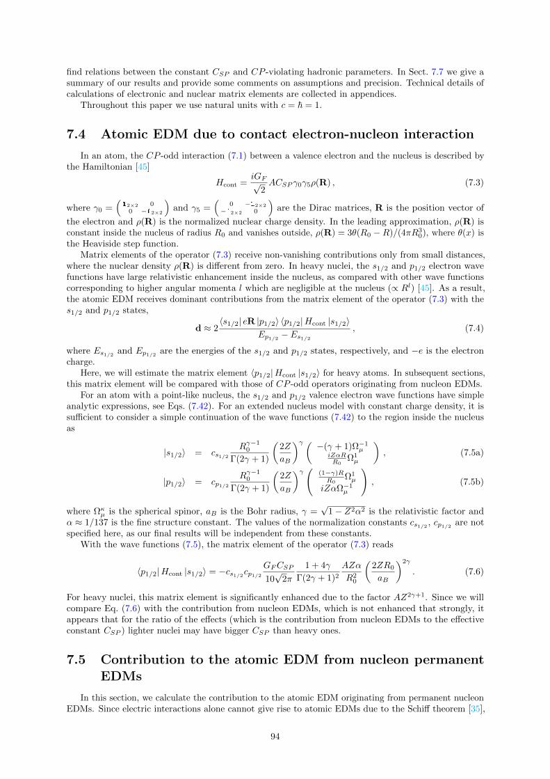
find relations between the constant CSP and CP -violating hadronic parameters. In Sect. 7.7 we give asummary of our results and provide some comments on assumptions and precision. Technical details ofcalculations of electronic and nuclear matrix elements are collected in appendices.

Throughout this paper we use natural units with c = ~ = 1.

7.4 Atomic EDM due to contact electron-nucleon interaction

In an atom, the CP -odd interaction (7.1) between a valence electron and the nucleus is described bythe Hamiltonian [45]

Hcont =iGF√

2ACSP γ0γ5ρ(R) , (7.3)

where γ0 =(12×2 0

0 −12×2

)and γ5 =

(0 −12×2

−12×2 0

)are the Dirac matrices, R is the position vector of

the electron and ρ(R) is the normalized nuclear charge density. In the leading approximation, ρ(R) isconstant inside the nucleus of radius R0 and vanishes outside, ρ(R) = 3θ(R0 −R)/(4πR3

0), where θ(x) isthe Heaviside step function.

Matrix elements of the operator (7.3) receive non-vanishing contributions only from small distances,where the nuclear density ρ(R) is different from zero. In heavy nuclei, the s1/2 and p1/2 electron wavefunctions have large relativistic enhancement inside the nucleus, as compared with other wave functionscorresponding to higher angular momenta l which are negligible at the nucleus (∝ Rl) [45]. As a result,the atomic EDM receives dominant contributions from the matrix element of the operator (7.3) with thes1/2 and p1/2 states,

d ≈ 2〈s1/2| eR |p1/2〉 〈p1/2|Hcont |s1/2〉

Ep1/2 − Es1/2, (7.4)

where Es1/2 and Ep1/2 are the energies of the s1/2 and p1/2 states, respectively, and −e is the electroncharge.

Here, we will estimate the matrix element 〈p1/2|Hcont |s1/2〉 for heavy atoms. In subsequent sections,this matrix element will be compared with those of CP -odd operators originating from nucleon EDMs.

For an atom with a point-like nucleus, the s1/2 and p1/2 valence electron wave functions have simpleanalytic expressions, see Eqs. (7.42). For an extended nucleus model with constant charge density, it issufficient to consider a simple continuation of the wave functions (7.42) to the region inside the nucleusas

|s1/2〉 = cs1/2Rγ−1

0

Γ(2γ + 1)

(2Z

aB

)γ ( −(γ + 1)Ω−1µ

iZαRR0

Ω1µ

), (7.5a)

|p1/2〉 = cp1/2Rγ−1

0

Γ(2γ + 1)

(2Z

aB

)γ ( (1−γ)RR0

Ω1µ

iZαΩ−1µ

), (7.5b)

where Ωκµ is the spherical spinor, aB is the Bohr radius, γ =

√1− Z2α2 is the relativistic factor and

α ≈ 1/137 is the fine structure constant. The values of the normalization constants cs1/2 , cp1/2 are notspecified here, as our final results will be independent from these constants.

With the wave functions (7.5), the matrix element of the operator (7.3) reads

〈p1/2|Hcont |s1/2〉 = −cs1/2cp1/2GFCSP

10√

2π

1 + 4γ

Γ(2γ + 1)2

AZα

R20

(2ZR0

aB

)2γ

. (7.6)

For heavy nuclei, this matrix element is significantly enhanced due to the factor AZ2γ+1. Since we willcompare Eq. (7.6) with the contribution from nucleon EDMs, which is not enhanced that strongly, itappears that for the ratio of the effects (which is the contribution from nucleon EDMs to the effectiveconstant CSP ) lighter nuclei may have bigger CSP than heavy ones.

7.5 Contribution to the atomic EDM from nucleon permanentEDMs

In this section, we calculate the contribution to the atomic EDM originating from permanent nucleonEDMs. Since electric interactions alone cannot give rise to atomic EDMs due to the Schiff theorem [35],

94

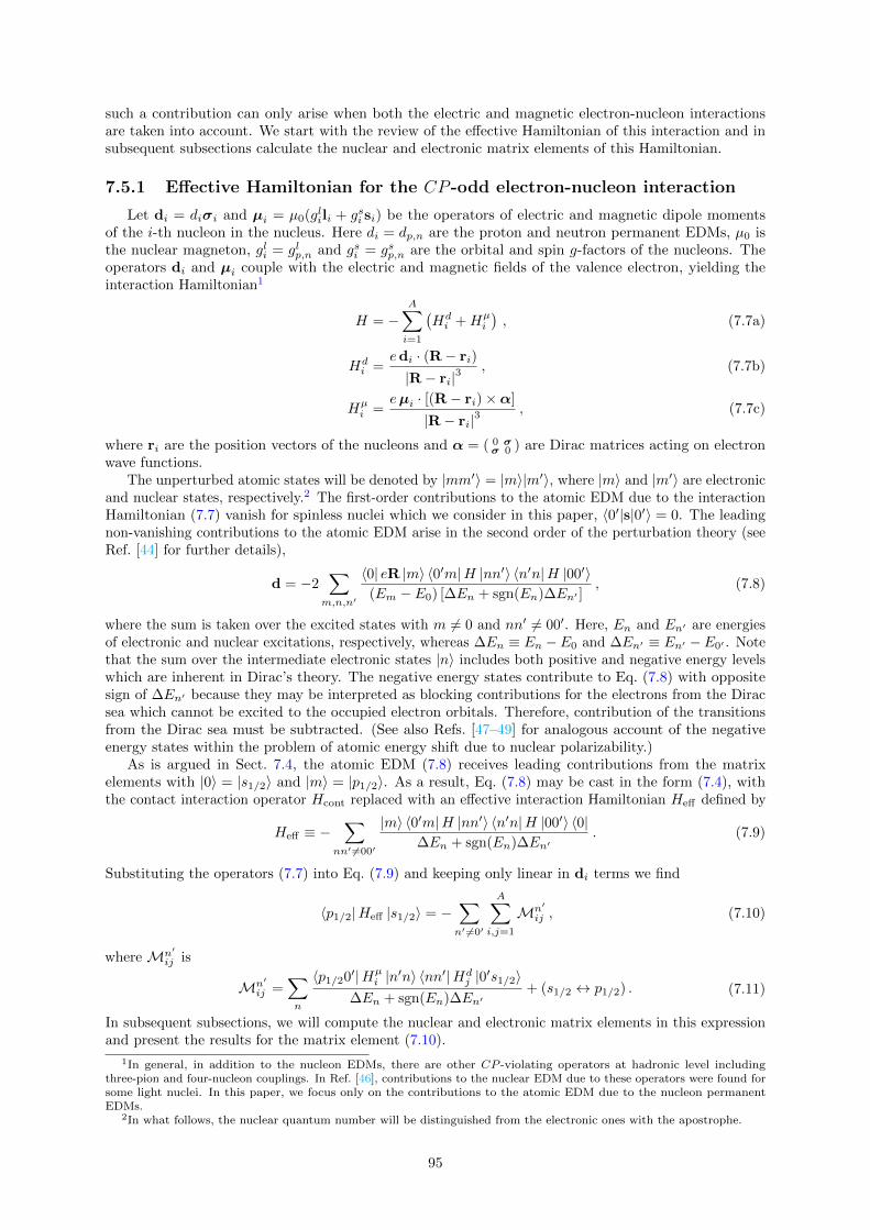
such a contribution can only arise when both the electric and magnetic electron-nucleon interactionsare taken into account. We start with the review of the effective Hamiltonian of this interaction and insubsequent subsections calculate the nuclear and electronic matrix elements of this Hamiltonian.

7.5.1 Effective Hamiltonian for the CP -odd electron-nucleon interaction

Let di = diσi and µi = µ0(glili + gsi si) be the operators of electric and magnetic dipole momentsof the i-th nucleon in the nucleus. Here di = dp,n are the proton and neutron permanent EDMs, µ0 isthe nuclear magneton, gli = glp,n and gsi = gsp,n are the orbital and spin g-factors of the nucleons. Theoperators di and µi couple with the electric and magnetic fields of the valence electron, yielding theinteraction Hamiltonian1

H = −A∑i=1

(Hdi +Hµ

i

), (7.7a)

Hdi =

edi · (R− ri)

|R− ri|3, (7.7b)

Hµi =

eµi · [(R− ri)×α]

|R− ri|3, (7.7c)

where ri are the position vectors of the nucleons and α = ( 0 σσ 0 ) are Dirac matrices acting on electron

wave functions.The unperturbed atomic states will be denoted by |mm′〉 = |m〉|m′〉, where |m〉 and |m′〉 are electronic

and nuclear states, respectively.2 The first-order contributions to the atomic EDM due to the interactionHamiltonian (7.7) vanish for spinless nuclei which we consider in this paper, 〈0′|s|0′〉 = 0. The leadingnon-vanishing contributions to the atomic EDM arise in the second order of the perturbation theory (seeRef. [44] for further details),

d = −2∑m,n,n′

〈0| eR |m〉 〈0′m|H |nn′〉 〈n′n|H |00′〉(Em − E0) [∆En + sgn(En)∆En′ ]

, (7.8)

where the sum is taken over the excited states with m 6= 0 and nn′ 6= 00′. Here, En and En′ are energiesof electronic and nuclear excitations, respectively, whereas ∆En ≡ En −E0 and ∆En′ ≡ En′ −E0′ . Notethat the sum over the intermediate electronic states |n〉 includes both positive and negative energy levelswhich are inherent in Dirac’s theory. The negative energy states contribute to Eq. (7.8) with oppositesign of ∆En′ because they may be interpreted as blocking contributions for the electrons from the Diracsea which cannot be excited to the occupied electron orbitals. Therefore, contribution of the transitionsfrom the Dirac sea must be subtracted. (See also Refs. [47–49] for analogous account of the negativeenergy states within the problem of atomic energy shift due to nuclear polarizability.)

As is argued in Sect. 7.4, the atomic EDM (7.8) receives leading contributions from the matrixelements with |0〉 = |s1/2〉 and |m〉 = |p1/2〉. As a result, Eq. (7.8) may be cast in the form (7.4), withthe contact interaction operator Hcont replaced with an effective interaction Hamiltonian Heff defined by

Heff ≡ −∑

nn′ 6=00′

|m〉 〈0′m|H |nn′〉 〈n′n|H |00′〉 〈0|∆En + sgn(En)∆En′

. (7.9)

Substituting the operators (7.7) into Eq. (7.9) and keeping only linear in di terms we find

〈p1/2|Heff |s1/2〉 = −∑n′ 6=0′

A∑i,j=1

Mn′

ij , (7.10)

where Mn′

ij is

Mn′

ij =∑n

〈p1/20′|Hµi |n′n〉 〈nn′|Hd

j |0′s1/2〉∆En + sgn(En)∆En′

+ (s1/2 ↔ p1/2) . (7.11)

In subsequent subsections, we will compute the nuclear and electronic matrix elements in this expressionand present the results for the matrix element (7.10).

1In general, in addition to the nucleon EDMs, there are other CP -violating operators at hadronic level includingthree-pion and four-nucleon couplings. In Ref. [46], contributions to the nuclear EDM due to these operators were found forsome light nuclei. In this paper, we focus only on the contributions to the atomic EDM due to the nucleon permanentEDMs.

2In what follows, the nuclear quantum number will be distinguished from the electronic ones with the apostrophe.

95

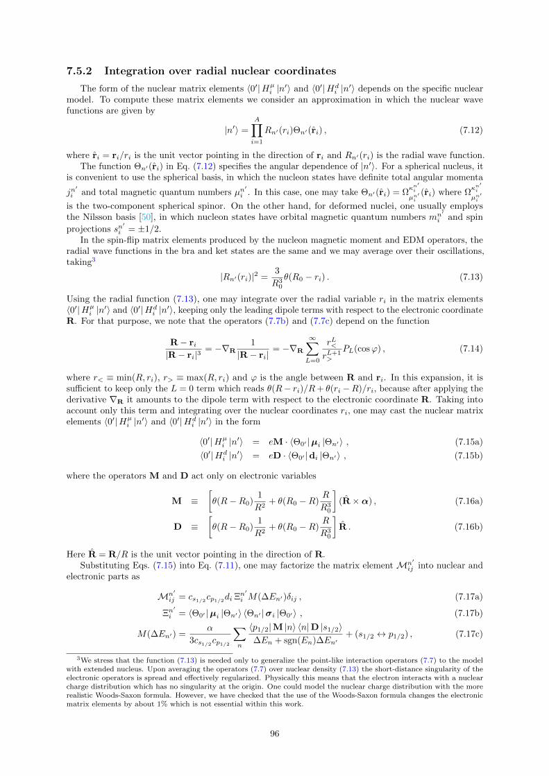
7.5.2 Integration over radial nuclear coordinates

The form of the nuclear matrix elements 〈0′|Hµi |n′〉 and 〈0′|Hd

i |n′〉 depends on the specific nuclearmodel. To compute these matrix elements we consider an approximation in which the nuclear wavefunctions are given by

|n′〉 =

A∏i=1

Rn′(ri)Θn′(ri) , (7.12)

where ri = ri/ri is the unit vector pointing in the direction of ri and Rn′(ri) is the radial wave function.The function Θn′(ri) in Eq. (7.12) specifies the angular dependence of |n′〉. For a spherical nucleus, it

is convenient to use the spherical basis, in which the nucleon states have definite total angular momenta

jn′

i and total magnetic quantum numbers µn′

i . In this case, one may take Θn′(ri) = Ωκn′i

µn′i

(ri) where Ωκn′i

µn′i

is the two-component spherical spinor. On the other hand, for deformed nuclei, one usually employsthe Nilsson basis [50], in which nucleon states have orbital magnetic quantum numbers mn′

i and spin

projections sn′

i = ±1/2.In the spin-flip matrix elements produced by the nucleon magnetic moment and EDM operators, the

radial wave functions in the bra and ket states are the same and we may average over their oscillations,taking3

|Rn′(ri)|2 =3

R30

θ(R0 − ri) . (7.13)

Using the radial function (7.13), one may integrate over the radial variable ri in the matrix elements〈0′|Hµ

i |n′〉 and 〈0′|Hdi |n′〉, keeping only the leading dipole terms with respect to the electronic coordinate

R. For that purpose, we note that the operators (7.7b) and (7.7c) depend on the function

R− ri|R− ri|3

= −∇R1

|R− ri|= −∇R

∞∑L=0

rL<rL+1>

PL(cosϕ) , (7.14)

where r< ≡ min(R, ri), r> ≡ max(R, ri) and ϕ is the angle between R and ri. In this expansion, it issufficient to keep only the L = 0 term which reads θ(R− ri)/R+ θ(ri −R)/ri, because after applying thederivative ∇R it amounts to the dipole term with respect to the electronic coordinate R. Taking intoaccount only this term and integrating over the nuclear coordinates ri, one may cast the nuclear matrixelements 〈0′|Hµ

i |n′〉 and 〈0′|Hdi |n′〉 in the form

〈0′|Hµi |n

′〉 = eM · 〈Θ0′ |µi |Θn′〉 , (7.15a)

〈0′|Hdi |n′〉 = eD · 〈Θ0′ |di |Θn′〉 , (7.15b)

where the operators M and D act only on electronic variables

M ≡[θ(R−R0)

1

R2+ θ(R0 −R)

R

R30

](R×α) , (7.16a)

D ≡[θ(R−R0)

1

R2+ θ(R0 −R)

R

R30

]R . (7.16b)

Here R = R/R is the unit vector pointing in the direction of R.Substituting Eqs. (7.15) into Eq. (7.11), one may factorize the matrix element Mn′

ij into nuclear andelectronic parts as

Mn′

ij = cs1/2cp1/2di Ξn′

i M(∆En′)δij , (7.17a)

Ξn′

i = 〈Θ0′ |µi |Θn′〉 〈Θn′ |σi |Θ0′〉 , (7.17b)

M(∆En′) =α

3cs1/2cp1/2

∑n

〈p1/2|M |n〉 〈n|D |s1/2〉∆En + sgn(En)∆En′

+ (s1/2 ↔ p1/2) , (7.17c)

3We stress that the function (7.13) is needed only to generalize the point-like interaction operators (7.7) to the modelwith extended nucleus. Upon averaging the operators (7.7) over nuclear density (7.13) the short-distance singularity of theelectronic operators is spread and effectively regularized. Physically this means that the electron interacts with a nuclearcharge distribution which has no singularity at the origin. One could model the nuclear charge distribution with the morerealistic Woods-Saxon formula. However, we have checked that the use of the Woods-Saxon formula changes the electronicmatrix elements by about 1% which is not essential within this work.

96

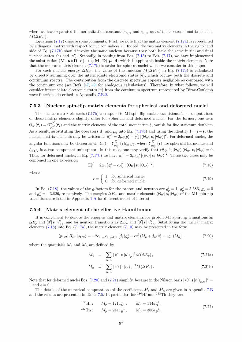
where we have separated the normalization constants cs1/2 and cp1/2 out of the electronic matrix elementM(∆En′).

Equations (7.17) deserve some comments. First, we note that the matrix element (7.17a) is representedby a diagonal matrix with respect to nucleon indices ij. Indeed, the two matrix elements in the right-handside of Eq. (7.17b) should involve the same nucleon because they both have the same initial and finalnuclear states |0′〉 and |n′〉. Secondly, in passing from Eqs. (7.15) to Eqs. (7.17), we have implementedthe substitution (M · µ)(D · d)→ 1

3 (M ·D)(µ · d) which is applicable inside the matrix elements. Notethat the nuclear matrix element (7.17b) is scalar for spinless nuclei which we consider in this paper.

For each nuclear energy ∆En′ , the value of the function M(∆En′) in Eq. (7.17c) is calculatedby directly summing over the intermediate electronic states |n〉, which occupy both the discrete andcontinuum spectra. The contribution from the discrete spectrum appears negligible as compared withthe continuum one (see Refs. [47, 49] for analogous calculations). Therefore, in what follows, we willconsider intermediate electronic states |n〉 from the continuum spectrum represented by Dirac-Coulombwave functions described in Appendix 7.B.2.

7.5.3 Nuclear spin-flip matrix elements for spherical and deformed nuclei

The nuclear matrix elements (7.17b) correspond to M1 spin-flip nuclear transitions. The computationsof these matrix elements slightly differ for spherical and deformed nuclei. For the former, one uses

Θn′(ri) = Ωκn′i

µn′i

(ri) and the matrix elements of the total momentum ji vanish for fine structure doublets.

As a result, substituting the operators di and µi into Eq. (7.17b) and using the identity l = j− s, the

nuclear matrix elements may be written as Ξn′

i = 2µ0(gsi − gli) |〈Θn′ | si |Θ0′〉|2. For deformed nuclei, the

angular functions may be chosen as Θn′(ri) = Yln′i

mn′i

(r)ζ±1/2, where Yln′i

mn′i

(r) are spherical harmonics and

ζ±1/2 is a two-component unit spinor. In this case, one may verify that 〈Θ0′ | li |Θn′〉 〈Θn′ | si |Θ0′〉 = 0.

Thus, for deformed nuclei, in Eq. (7.17b) we have Ξn′

i = 2µ0gsi |〈Θn′ | si |Θ0′〉|2. These two cases may be

combined in one expressionΞn′

i = 2µ0

(gsi − εgli

)| 〈Θ0′ | si |Θn′〉 |2 , (7.18)

where

ε =

1 for spherical nuclei0 for deformed nuclei.

(7.19)

In Eq. (7.18), the values of the g-factors for the proton and neutron are glp = 1, gsp = 5.586, gln = 0and gsn = −3.826, respectively. The energies ∆En′ and matrix elements 〈Θ0′ | si |Θn′〉 of the M1 spin-fliptransitions are listed in Appendix 7.A for different nuclei of interest.

7.5.4 Matrix element of the effective Hamiltonian

It is convenient to denote the energies and matrix elements for proton M1 spin-flip transitions as∆Ep and 〈0′| s |n′〉p, and for neutron transitions as ∆En and 〈0′| s |n′〉n. Substituting the nuclear matrixelements (7.18) into Eq. (7.17a), the matrix element (7.10) may be presented in the form

〈p1/2|Heff |s1/2〉 = −2cs1/2cp1/2µ0

[dp(g

sp − εglp)Mp + dn(gsn − εgln)Mn

], (7.20)

where the quantities Mp and Mn are defined by

Mp ≡∑∆Ep

| 〈0′| s |n′〉p |2M(∆Ep) , (7.21a)

Mn ≡∑∆En

| 〈0′| s |n′〉n |2M(∆En) . (7.21b)

Note that for deformed nuclei Eqs. (7.20) and (7.21) simplify, because in the Nilsson basis | 〈0′| s |n′〉p,n |2 =1 and ε = 0.

The details of the numerical computations of the coefficients Mp and Mn are given in Appendix 7.Band the results are presented in Table 7.5. In particular, for 180Hf and 232Th they are:

180Hf : Mp = 121a−1B , Mn = 114a−1

B ,232Th : Mp = 244a−1

B , Mn = 385a−1B .

(7.22)

97

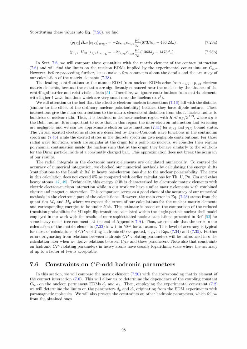
Substituting these values into Eq. (7.20), we find

〈p1/2|Heff |s1/2〉180Hf= −2cs1/2cp1/2

µ0

aB(673.7dp − 436.2dn) , (7.23a)

〈p1/2|Heff |s1/2〉232Th= −2cs1/2cp1/2

µ0

aB(1363dp − 1473dn) . (7.23b)

In Sect. 7.6, we will compare these quantities with the matrix element of the contact interaction(7.6) and will find the limits on the nucleon EDMs implied by the experimental constraints on CSP .However, before proceeding further, let us make a few comments about the details and the accuracy ofour calculation of the matrix elements (7.23).

The leading contributions to the atomic EDM from nucleon EDMs arise from s1/2 - p1/2 electronmatrix elements, because these states are significantly enhanced near the nucleus by the absence of thecentrifugal barrier and relativistic effects [51]. Therefore, we ignore contributions from matrix elementswith higher-l wave functions which are very small near the nucleus (∝ rl).

We call attention to the fact that the effective electron-nucleon interactions (7.16) fall with the distance(similar to the effect of the ordinary nuclear polarizability) because they have dipole nature. Theseinteractions give the main contributions to the matrix elements at distances from about nuclear radius tohundreds of nuclear radii. Thus, it is localised in the near-nucleus region with R aB/Z

1/3, where aB isthe Bohr radius. It is important to note that in this region the inter-electron interaction and screeningare negligible, and we can use approximate electron wave functions (7.41) for s1/2 and p1/2 bound states.The virtual excited electronic states are described by Dirac-Coulomb wave functions in the continuumspectrum (7.45) while the excited states in the discrete spectrum give negligible contributions. For thoseradial wave functions, which are singular at the origin for a point-like nucleus, we consider their regularpolynomial continuation inside the nucleus such that at the origin they behave similarly to the solutionsfor the Dirac particle inside of a constantly charged ball. This approximation does not break the accuracyof our results.

The radial integrals in the electronic matrix elements are calculated numerically. To control theaccuracy of numerical integration, we checked our numerical methods by calculating the energy shifts(contributions to the Lamb shifts) in heavy one-electron ions due to the nuclear polarizability. The errorin this calculation does not exceed 5% as compared with earlier calculations for Th, U, Pu, Cm and otherheavy atoms [47, 49]. Technically, this energy shift is characterised by electronic matrix elements withelectric electron-nucleon interaction while in our work we have similar matrix elements with combinedelectric and magnetic interaction. This comparison serves as a good check of the accuracy of our numericalmethods in the electronic part of the calculations. However, the main error in Eq. (7.23) stems from thequantities Mp and Mn where we expect the errors of our calculations for the nuclear matrix elementsand corresponding energies to be under 50%. This estimate is based on the comparison of the reducedtransition probabilities for M1 spin-flip transitions calculated within the single-particle nuclear shell modelemployed in our work with the results of more sophisticated nuclear calculations presented in Ref. [52] forsome heavy nuclei (see comments at the end of Appendix 7.A). Thus, we conclude that the error in ourcalculation of the matrix elements (7.23) is within 50% for all atoms. This level of accuracy is typicalfor most of calculations of CP -violating hadronic effects quoted, e.g., in Eqs. (7.34) and (7.35). Furthererrors originating from relations between hadronic CP -violating parameters will be introduced into thecalculation later when we derive relations between CSP and these parameters. Note also that constraintson hadronic CP -violating parameters in heavy atoms have usually logarithmic scale where the accuracyof up to a factor of two is acceptable.

7.6 Constraints on CP -odd hadronic parameters

In this section, we will compare the matrix element (7.20) with the corresponding matrix element ofthe contact interaction (7.6). This will allow us to determine the dependence of the coupling constantCSP on the nucleon permanent EDMs dp and dn. Then, employing the experimental constraint (7.2)we will determine the limits on the parameters dp and dn originating from the EDM experiments withparamagnetic molecules. We will also present the constraints on other hadronic parameters, which followfrom the obtained ones.

98

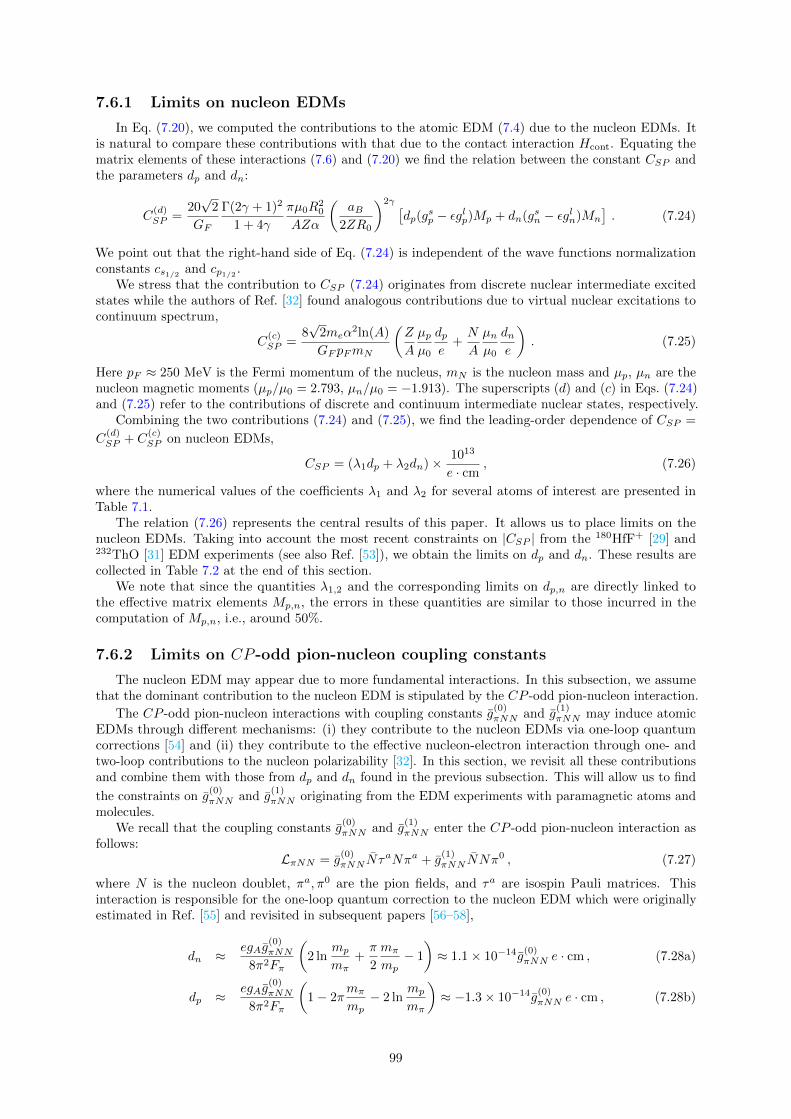
7.6.1 Limits on nucleon EDMs

In Eq. (7.20), we computed the contributions to the atomic EDM (7.4) due to the nucleon EDMs. Itis natural to compare these contributions with that due to the contact interaction Hcont. Equating thematrix elements of these interactions (7.6) and (7.20) we find the relation between the constant CSP andthe parameters dp and dn:

C(d)SP =

20√

2

GF

Γ(2γ + 1)2

1 + 4γ

πµ0R20

AZα

(aB

2ZR0

)2γ [dp(g

sp − εglp)Mp + dn(gsn − εgln)Mn

]. (7.24)

We point out that the right-hand side of Eq. (7.24) is independent of the wave functions normalizationconstants cs1/2 and cp1/2 .

We stress that the contribution to CSP (7.24) originates from discrete nuclear intermediate excitedstates while the authors of Ref. [32] found analogous contributions due to virtual nuclear excitations tocontinuum spectrum,

C(c)SP =

8√

2meα2ln(A)

GF pFmN

(Z

A

µpµ0

dpe

+N

A

µnµ0

dne

). (7.25)

Here pF ≈ 250 MeV is the Fermi momentum of the nucleus, mN is the nucleon mass and µp, µn are thenucleon magnetic moments (µp/µ0 = 2.793, µn/µ0 = −1.913). The superscripts (d) and (c) in Eqs. (7.24)and (7.25) refer to the contributions of discrete and continuum intermediate nuclear states, respectively.

Combining the two contributions (7.24) and (7.25), we find the leading-order dependence of CSP =

C(d)SP + C

(c)SP on nucleon EDMs,

CSP = (λ1dp + λ2dn)× 1013

e · cm, (7.26)

where the numerical values of the coefficients λ1 and λ2 for several atoms of interest are presented inTable 7.1.

The relation (7.26) represents the central results of this paper. It allows us to place limits on thenucleon EDMs. Taking into account the most recent constraints on |CSP | from the 180HfF+ [29] and232ThO [31] EDM experiments (see also Ref. [53]), we obtain the limits on dp and dn. These results arecollected in Table 7.2 at the end of this section.

We note that since the quantities λ1,2 and the corresponding limits on dp,n are directly linked tothe effective matrix elements Mp,n, the errors in these quantities are similar to those incurred in thecomputation of Mp,n, i.e., around 50%.

7.6.2 Limits on CP -odd pion-nucleon coupling constants

The nucleon EDM may appear due to more fundamental interactions. In this subsection, we assumethat the dominant contribution to the nucleon EDM is stipulated by the CP -odd pion-nucleon interaction.

The CP -odd pion-nucleon interactions with coupling constants g(0)πNN and g

(1)πNN may induce atomic

EDMs through different mechanisms: (i) they contribute to the nucleon EDMs via one-loop quantumcorrections [54] and (ii) they contribute to the effective nucleon-electron interaction through one- andtwo-loop contributions to the nucleon polarizability [32]. In this section, we revisit all these contributionsand combine them with those from dp and dn found in the previous subsection. This will allow us to find

the constraints on g(0)πNN and g

(1)πNN originating from the EDM experiments with paramagnetic atoms and

molecules.We recall that the coupling constants g

(0)πNN and g

(1)πNN enter the CP -odd pion-nucleon interaction as

follows:LπNN = g

(0)πNN Nτ

aNπa + g(1)πNN NNπ

0 , (7.27)

where N is the nucleon doublet, πa, π0 are the pion fields, and τa are isospin Pauli matrices. Thisinteraction is responsible for the one-loop quantum correction to the nucleon EDM which were originallyestimated in Ref. [55] and revisited in subsequent papers [56–58],

dn ≈egAg

(0)πNN

8π2Fπ

(2 ln

mp

mπ+π

2

mπ

mp− 1

)≈ 1.1× 10−14g

(0)πNN e · cm , (7.28a)

dp ≈egAg

(0)πNN

8π2Fπ

(1− 2π

mπ

mp− 2 ln

mp

mπ

)≈ −1.3× 10−14g

(0)πNN e · cm , (7.28b)

99

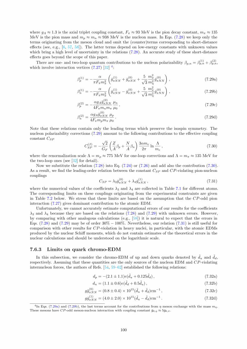
where gA ≈ 1.3 is the axial triplet coupling constant, Fπ ≈ 93 MeV is the pion decay constant, mπ ≈ 135MeV is the pion mass and mp ≈ mn ≈ 938 MeV is the nucleon mass. In Eqs. (7.28) we keep only theterms originating from the meson cloud and omit the (counter)terms corresponding to short-distanceeffects (see, e.g., [6, 57, 58]). The latter terms depend on low-energy constants with unknown valueswhich bring a high level of uncertainty in the relations (7.28). An accurate study of these short-distanceeffects goes beyond the scope of this paper.

There are one- and two-loop quantum contributions to the nucleon polarizability βp,n = β(1)p,n + β

(2)p,n,

which involve interaction vertices (7.27) [32] 4:

β(1)p = − α

πFπm2π

(g

(1)πNN + g

(0)πNN +

5√3

m2π

m2η

g(0)πNN

), (7.29a)

β(1)n = − α

πFπm2π

(g

(1)πNN − g

(0)πNN +

5√3

m2π

m2η

g(0)πNN

), (7.29b)

β(2)p = −

αgAg(0)πNN

4Fπmnmπ

µnµ0

, (7.29c)

β(2)n =

αgAg(0)πNN

4Fπmpmπ

µpµ0

. (7.29d)

Note that these relations contain only the leading terms which preserve the isospin symmetry. Thenucleon polarizability corrections (7.29) amount to the following contributions to the effective couplingconstant CSP

C(β)SP = −

√2

GF

(Z

Aβp +

N

Aβn

)3αme

2πln

Λ

me, (7.30)

where the renormalization scale Λ = mρ ≈ 775 MeV for one-loop corrections and Λ = mπ ≈ 135 MeV forthe two-loop ones (see [32] for detail).

Now we substitute the relation (7.28) into Eq. (7.24) or (7.26) and add also the contribution (7.30).As a result, we find the leading-order relation between the constant CSP and CP -violating pion-nucleoncouplings

CSP = λ3g(0)πNN + λ4g

(1)πNN , (7.31)

where the numerical values of the coefficients λ3 and λ4 are collected in Table 7.1 for different atoms.The corresponding limits on these couplings originating from the experimental constraints are givenin Table 7.2 below. We stress that these limits are based on the assumption that the CP -odd pioninteraction (7.27) gives dominant contribution to the atomic EDM.

Unfortunately, we cannot accurately estimate computational errors of our results for the coefficientsλ3 and λ4 because they are based on the relations (7.28) and (7.29) with unknown errors. However,by comparing with other analogous calculations (e.g., [58]) it is natural to expect that the errors inEqs. (7.28) and (7.29) may be of order 30%− 100%. Nevertheless, our relation (7.31) is still useful forcomparison with other results for CP -violation in heavy nuclei, in particular, with the atomic EDMsproduced by the nuclear Schiff moments, which do not contain estimates of the theoretical errors in thenuclear calculations and should be understood on the logarithmic scale.

7.6.3 Limits on quark chromo-EDM

In this subsection, we consider the chromo-EDM of up and down quarks denoted by du and dd,respectively. Assuming that these quantities are the only sources of the nucleon EDM and CP -violatinginternucleon forces, the authors of Refs. [54, 59–62] established the following relations:

dp = −(2.1± 1.1)e(du + 0.125dd) , (7.32a)

dn = (1.1± 0.6)e(dd + 0.5du) , (7.32b)

gg(0)πNN = (0.8± 0.4)× 1015(du + dd)cm−1 , (7.32c)

gg(1)πNN = (4.0± 2.0)× 1015(du − dd)cm−1 . (7.32d)

4In Eqs. (7.29a) and (7.29b), the last terms account for the contributions from η meson exchange with the mass mη.These mesons have CP -odd meson-nucleon interaction with coupling constant g0,η ≈ 5g0,π .

100

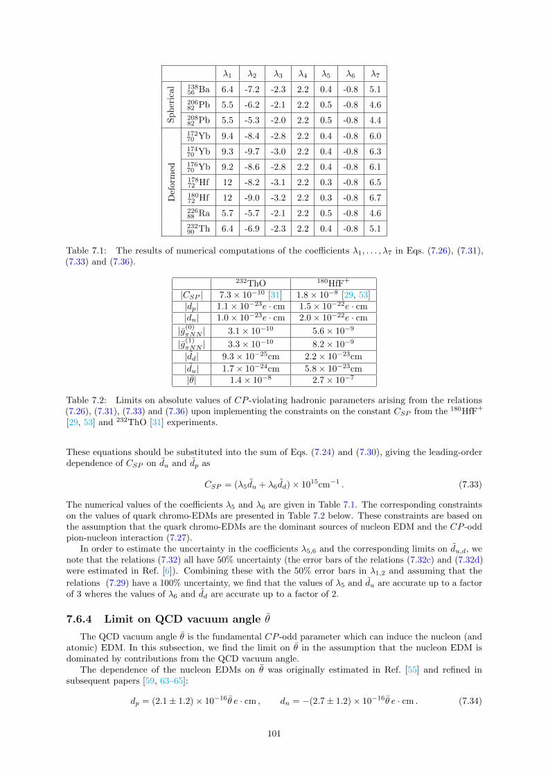
λ1 λ2 λ3 λ4 λ5 λ6 λ7

Sp

her

ical 138

56 Ba 6.4 -7.2 -2.3 2.2 0.4 -0.8 5.1

20682 Pb 5.5 -6.2 -2.1 2.2 0.5 -0.8 4.6

20882 Pb 5.5 -5.3 -2.0 2.2 0.5 -0.8 4.4

Def

orm

ed

17270 Yb 9.4 -8.4 -2.8 2.2 0.4 -0.8 6.0

17470 Yb 9.3 -9.7 -3.0 2.2 0.4 -0.8 6.3

17670 Yb 9.2 -8.6 -2.8 2.2 0.4 -0.8 6.1

17872 Hf 12 -8.2 -3.1 2.2 0.3 -0.8 6.5

18072 Hf 12 -9.0 -3.2 2.2 0.3 -0.8 6.7

22688 Ra 5.7 -5.7 -2.1 2.2 0.5 -0.8 4.6

23290 Th 6.4 -6.9 -2.3 2.2 0.4 -0.8 5.1

Table 7.1: The results of numerical computations of the coefficients λ1, . . . , λ7 in Eqs. (7.26), (7.31),(7.33) and (7.36).

232ThO 180HfF+

|CSP | 7.3× 10−10 [31] 1.8× 10−8 [29, 53]|dp| 1.1× 10−23e · cm 1.5× 10−22e · cm|dn| 1.0× 10−23e · cm 2.0× 10−22e · cm

|g(0)πNN | 3.1× 10−10 5.6× 10−9

|g(1)πNN | 3.3× 10−10 8.2× 10−9

|dd| 9.3× 10−25cm 2.2× 10−23cm

|du| 1.7× 10−24cm 5.8× 10−23cm|θ| 1.4× 10−8 2.7× 10−7

Table 7.2: Limits on absolute values of CP -violating hadronic parameters arising from the relations(7.26), (7.31), (7.33) and (7.36) upon implementing the constraints on the constant CSP from the 180HfF+

[29, 53] and 232ThO [31] experiments.

These equations should be substituted into the sum of Eqs. (7.24) and (7.30), giving the leading-orderdependence of CSP on du and dp as

CSP = (λ5du + λ6dd)× 1015cm−1 . (7.33)

The numerical values of the coefficients λ5 and λ6 are given in Table 7.1. The corresponding constraintson the values of quark chromo-EDMs are presented in Table 7.2 below. These constraints are based onthe assumption that the quark chromo-EDMs are the dominant sources of nucleon EDM and the CP -oddpion-nucleon interaction (7.27).

In order to estimate the uncertainty in the coefficients λ5,6 and the corresponding limits on du,d, wenote that the relations (7.32) all have 50% uncertainty (the error bars of the relations (7.32c) and (7.32d)were estimated in Ref. [6]). Combining these with the 50% error bars in λ1,2 and assuming that the

relations (7.29) have a 100% uncertainty, we find that the values of λ5 and du are accurate up to a factorof 3 wheres the values of λ6 and dd are accurate up to a factor of 2.

7.6.4 Limit on QCD vacuum angle θ

The QCD vacuum angle θ is the fundamental CP -odd parameter which can induce the nucleon (andatomic) EDM. In this subsection, we find the limit on θ in the assumption that the nucleon EDM isdominated by contributions from the QCD vacuum angle.

The dependence of the nucleon EDMs on θ was originally estimated in Ref. [55] and refined insubsequent papers [59, 63–65]:

dp = (2.1± 1.2)× 10−16θ e · cm , dn = −(2.7± 1.2)× 10−16θ e · cm . (7.34)

101

The pion-nucleon coupling constants g(0)πNN and g

(1)πNN can also be expressed via θ as [54, 63, 66] (see also

Refs. [6, 65] for reviews5)

g(0)πNN = −(15.5± 2.5)× 10−3 θ , g

(1)πNN = (3.4± 2)× 10−3 θ . (7.35)

Substituting these relations into the sum of Eqs. (7.24) and (7.30) we represent CSP in terms of θ

CSP = λ7 × 10−2θ , (7.36)

where the value of the constant λ7 is given in Table 7.1 for different atoms. In particular, with the use ofthe corresponding value for 232Th, the experimental constraint on CSP (7.2) implies

|θ| < 1.4× 10−8 . (7.37)

This constraint is close to the result advocated in the recent paper [32].Using the uncertainties in Eqs. (7.34) and (7.35) and assuming that the relations (7.29) have a 100%

uncertainty, we find that the error bars in the relation (7.36) and the corresponding limit (7.37) are about40%− 50%.

7.7 Summary and discussion

In this paper, we demonstrated that the experiments measuring the electron electric dipole momentwith paramagnetic atoms and molecules are also sensitive to nucleon EDMs. Dominant contributions tothe atomic EDM in such atoms arise from the combined electric and magnetic electron-nucleus interaction.Taking into account nuclear structure effects, we derived the leading-order relations (7.26) between theelectron-nucleus contact interaction constant CSP and nucleon permanent EDMs dp and dn. As a result,the constraint (7.2) on the parameter CSP allows us to find limits on nucleon EDMs arising from theexperiments with paramagnetic molecules:

|dp| < 1.1× 10−23e · cm , |dn| < 1.0× 10−23e · cm . (7.38)

It is instructive to compare these limits with the currently accepted ones. In particular, our limit on theneutron EDM obtained from the results of experiments with paramagnetic molecules is almost three orderof magnitude weaker than the recent experimental measurements of EDM of neutron |dn| < 1.8×10−26e·cm[67]. However, for the proton EDM our limit (7.38) is just about 20 times weaker than the recent constrainton this parameter |dp| < 5× 10−25e · cm [68] which was based on the measurements on EDM of 199Hgatom [14].6 Remarkably, the constraint (7.38) on the proton EDM is nearly 30 times more stringent thanthat found in recent 129Xe EDM experiments [70, 71]. This sensitivity of eEDM experiments to hadronicCP -violating parameters is actually very impressive. We expect that further improvement of accuracy inthe experiments with paramagnetic molecules would push these limits.

The nucleon EDM may be expressed via more fundamental CP -violating parameters such as CP -odd

pion-nucleon coupling constants g(0,1)πNN , quark chromo-EDMs du,d and the QCD vacuum angle θ. This

allows us to find the leading-order dependence of the contact interaction coupling constant CSP on theseparameters. The results are represented by Eqs. (7.31), (7.33) and (7.36) with coefficients λ3, . . . , λ7

given in Table 7.1. The corresponding limits arising on these parameters from the experiments [29] and[31] are presented in Table 7.2. In particular, the QCD vacuum angle is limited as |θ| < 1.4 × 10−8

which is approximately two orders of magnitude weaker than the currently accepted constraint fromneutron and Hg atom EDM experiments |θ| < 10−10 [72], but is nearly three times more stringent thanthe corresponding bounds from 129Xe EDM experiments [70, 71]. Note that the limits presented abovedo not include theoretical errors which often are unknown (see, e.g., calculation of the 199Hg nuclearSchiff moment in Ref. [73] where different interaction models give different sign of the result). Our errorestimates are presented after corresponding formulas. In particular, for the limit on the nucleon EDMsdp,n and the QCD angle θ, the error is about 40-50% while the limit on the up quark chromo-EDM du iscorrect up to a factor of 3 and the limit on the down quark chromo-EDM is correct up to a factor of 2.

We stress that obtained in this paper contributions to CSP from nucleon EDMs are independent fromand additional to those found in Ref. [32], although they originate from the same combined electric and

5We point out that the signs in the relations (103) and (104) between g(0,1)πNN and θ quoted in Ref. [6] are inconsistent

with the definition of LπNN presented in that review.6Note that this constraint is approximately two times weaker than that in Ref. [69] because the authors of Ref. [68]

revisited earlier calculations of nuclear Shiff moments.

102

magnetic electron-nucleon interaction. Indeed, the authors of the paper [32] took into account virtualnuclear transitions from bound states to continuum for all nucleons in the nucleus, so it increases withthe nucleon number A. In our paper, in contrast, we consider virtual nuclear transitions to excited boundnuclear states for several external shell nucleons which can flip their spins. This contribution is enhancedby the small energy denominators and large matrix elements of the spin operator between the spin-orbitdoublet components. As we demonstrate in this paper, accounting these M1 nuclear spin-flip transitionsapproximately doubles the results presented in Ref. [32].

To conclude, we expect that the obtained in this paper results may place more stringent limits onCP -violating hadronic parameters once improved constraints on CSP are available from next generationsof eEDM experiments [10, 11, 29–31, 74]. Note that the sensitivity in these experiments improved by twoorders of magnitude during the last decade.

Acknowledgements

This work was supported by the Australian Research Council Grants No. DP150101405 andDP200100150 and the Gutenberg Fellowship. We thank Vladimir Dmitriev, Maxim Pospelov, Adam Ritz,Yevgeny Stadnik and Anna Viatkina for useful discussions.

7.A Nuclear energies and matrix elements

In this appendix, we estimate the matrix elements and corresponding energies of nuclear M1 spin-flipsingle-particle transitions. The details of these computations slightly differ for (nearly) spherical anddeformed nuclei. Therefore, we consider these two cases separately.

7.A.1 Spherical nuclei

In this section, we focus on the 208Pb, 206Pb and 138Ba nuclei, which are nearly spherical, i.e., theyhave deformation δ < 0.1. For these nuclei, proton and neutron single-particle states may be labeledas |n, l, j,m〉, where n is the oscillator quantum number, l and j are the orbital and total momentumnumbers, m is magnetic quantum number. In this basis, the nuclear spin operator s provides transitionsbetween fine structure doublets.

In the 208Pb nucleus, the non-vanishing matrix elements of the spin operator are 〈5h 92 |s|5h

112 〉

for protons and 〈6i 112 |s|6i

132 〉 for neutrons. The isotope 206Pb has additional contributions from the

〈5p 12 |s|5p

32 〉 neutron matrix elements. For 138Ba, non-vanishing proton contributions arise from the

matrix elements 〈4d 32 |s|4d

52 〉 and 〈4g 9

2 |s|4g72 〉 whereas neutron contributions come from 〈5h 9

2 |s|5h112 〉.

All these matrix elements may be calculated using the properties of spherical spinors (see, e.g., Ref. [75]).The energies of all these transitions may be estimated with the use of Fig. 5 in Ref. [76]. When theenergies are (nearly) degenerate, we give the sum of matrix elements corresponding to the same energy. InTable 7.3 below, we collect the values of such matrix elements with the corresponding energies for 208Pb,206Pb and 138Ba. The value of the nuclear radius R0 is calculated according to the empirical formula:

R0 = 1.2A1/3 fm . (7.39)

For reference, the values of the deformation parameter δ are also presented.

7.A.2 Deformed nuclei

For deformed heavy nuclei with δ > 0.1, it is convenient to use the Nilsson basis [50, 76], whereinproton and neutron single-particle states are labeled with |n3, n⊥,Λ,Ω〉, where n3 and n⊥ are the oscillatorquantum numbers, Λ and Ω are the projections of angular and total momenta on the deformation axis.Note that Ω = Λ + Σ where Σ is the projection of the nucleon’s spin on the deformation axis. Thedependence of the energy levels on the deformation parameter δ in this model may be inferred from Fig. 5in Ref. [76]. From such dependence, one may estimate the energies of the spin-flip transitions. Note thatin the basis |n3, n⊥,Λ,Ω〉, each M1 spin-flip matrix element is 〈m′| s+ |0′〉 = 1, and the correspondingenergy level is doubly degenerate since each quantum number Σ corresponds to ±Λ.

The single-nucleon spin-flip M1 transition energies ∆En′ , the deformation parameters δ and thenuclear radii R0 for several nuclei of interest are presented in Table 7.4.

103

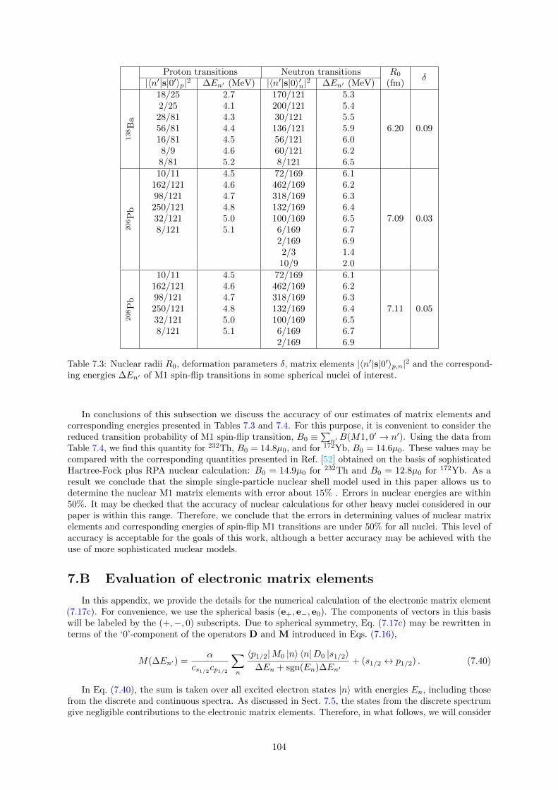
Proton transitions Neutron transitions R0 δ|〈n′|s|0′〉p|2 ∆En′ (MeV) |〈n′|s|0〉′n|2 ∆En′ (MeV) (fm)

138B

a

18/25 2.7 170/121 5.3

6.20 0.09

2/25 4.1 200/121 5.428/81 4.3 30/121 5.556/81 4.4 136/121 5.916/81 4.5 56/121 6.08/9 4.6 60/121 6.28/81 5.2 8/121 6.5

206P

b

10/11 4.5 72/169 6.1

7.09 0.03

162/121 4.6 462/169 6.298/121 4.7 318/169 6.3250/121 4.8 132/169 6.432/121 5.0 100/169 6.58/121 5.1 6/169 6.7

2/169 6.92/3 1.410/9 2.0

208P

b

10/11 4.5 72/169 6.1

7.11 0.05

162/121 4.6 462/169 6.298/121 4.7 318/169 6.3250/121 4.8 132/169 6.432/121 5.0 100/169 6.58/121 5.1 6/169 6.7

2/169 6.9

Table 7.3: Nuclear radii R0, deformation parameters δ, matrix elements |〈n′|s|0′〉p,n|2 and the correspond-ing energies ∆En′ of M1 spin-flip transitions in some spherical nuclei of interest.

In conclusions of this subsection we discuss the accuracy of our estimates of matrix elements andcorresponding energies presented in Tables 7.3 and 7.4. For this purpose, it is convenient to consider thereduced transition probability of M1 spin-flip transition, B0 ≡

∑n′ B(M1, 0′ → n′). Using the data from

Table 7.4, we find this quantity for 232Th, B0 = 14.8µ0, and for 172Yb, B0 = 14.6µ0. These values may becompared with the corresponding quantities presented in Ref. [52] obtained on the basis of sophisticatedHartree-Fock plus RPA nuclear calculation: B0 = 14.9µ0 for 232Th and B0 = 12.8µ0 for 172Yb. As aresult we conclude that the simple single-particle nuclear shell model used in this paper allows us todetermine the nuclear M1 matrix elements with error about 15% . Errors in nuclear energies are within50%. It may be checked that the accuracy of nuclear calculations for other heavy nuclei considered in ourpaper is within this range. Therefore, we conclude that the errors in determining values of nuclear matrixelements and corresponding energies of spin-flip M1 transitions are under 50% for all nuclei. This level ofaccuracy is acceptable for the goals of this work, although a better accuracy may be achieved with theuse of more sophisticated nuclear models.

7.B Evaluation of electronic matrix elements

In this appendix, we provide the details for the numerical calculation of the electronic matrix element(7.17c). For convenience, we use the spherical basis (e+, e−, e0). The components of vectors in this basiswill be labeled by the (+,−, 0) subscripts. Due to spherical symmetry, Eq. (7.17c) may be rewritten interms of the ‘0’-component of the operators D and M introduced in Eqs. (7.16),

M(∆En′) =α

cs1/2cp1/2

∑n

〈p1/2|M0 |n〉 〈n|D0 |s1/2〉∆En + sgn(En)∆En′

+ (s1/2 ↔ p1/2) . (7.40)

In Eq. (7.40), the sum is taken over all excited electron states |n〉 with energies En, including thosefrom the discrete and continuous spectra. As discussed in Sect. 7.5, the states from the discrete spectrumgive negligible contributions to the electronic matrix elements. Therefore, in what follows, we will consider

104

Proton transitions Neutron transitions R0 δTransition ∆En′ (MeV) Transition ∆En′ (MeV) (fm)

172Y

b

|523 72 〉 → |523 5

2 〉 4.5 |651 32 〉 → |651 1

2 〉 3.9

6.67 0.31|532 5

2 〉 → |532 32 〉 4.0 |642 5

2 〉 → |642 32 〉 4.5

|541 32 〉 → |541 1

2 〉 4.5 |633 72 〉 → |633 5

2 〉 5.0|404 9

2 〉 → |404 72 〉 4.1 |505 11

2 〉 → |505 92 〉 5.1

|514 92 〉 → |514 7

2 〉 4.6

174Y

b

|523 72 〉 → |523 5

2 〉 4.5 |651 32 〉 → |651 1

2 〉 3.9

6.70 0.31

|532 52 〉 → |532 3

2 〉 4.0 |642 52 〉 → |642 3

2 〉 4.5|541 3

2 〉 → |541 12 〉 4.5 |633 7

2 〉 → |633 52 〉 5.0

|404 92 〉 → |404 7

2 〉 4.1 |505 112 〉 → |505 9

2 〉 5.1|514 9

2 〉 → |514 72 〉 4.6

|512 52 〉 → |512 3

2 〉 2.4

176Y

b

|523 72 〉 → |523 5

2 〉 4.5 |651 32 〉 → |651 1

2 〉 4.2

6.72 0.29|532 5

2 〉 → |532 32 〉 4.1 |642 5

2 〉 → |642 32 〉 4.5

|541 32 〉 → |541 1

2 〉 4.5 |633 72 〉 → |633 5

2 〉 5.0|404 9

2 〉 → |404 72 〉 4.0 |505 11

2 〉 → |505 92 〉 5.2

|512 52 〉 → |512 3

2 〉 2.4

178H

f

|523 72 〉 → |523 5

2 〉 4.4 |505 112 〉 → |505 9

2 〉 4.2

6.75 0.26|532 5

2 〉 → |532 32 〉 4.1 |512 5

2 〉 → |512 32 〉 2.4

|541 32 〉 → |541 1

2 〉 4.1 |633 72 〉 → |633 5

2 〉 5.0|402 5

2 〉 → |402 32 〉 1.9 |642 5

2 〉 → |642 32 〉 4.6

|411 32 〉 → |411 1

2 〉 1.4 |631 32 〉 → |631 1

2 〉 7.8

180H

f

|523 72 〉 → |523 5

2 〉 4.4 |505 112 〉 → |505 9

2 〉 4.2

6.80 0.25

|532 52 〉 → |532 3

2 〉 4.1 |512 52 〉 → |512 3

2 〉 2.4|541 3

2 〉 → |541 12 〉 4.1 |624 9

2 〉 → |624 72 〉 5.3

|402 52 〉 → |402 3

2 〉 1.9 |633 72 〉 → |633 5

2 〉 5.0|411 3

2 〉 → |411 12 〉 1.4 |642 5

2 〉 → |642 32 〉 4.6

|631 32 〉 → |631 1

2 〉 7.8

226R

a

|523 72 〉 → |523 5

2 〉 4.3 |624 92 〉 → |624 7

2 〉 5.0

7.31 0.20|514 9

2 〉 → |514 72 〉 4.4 |615 11

2 〉 → |615 92 〉 5.0

|505 112 〉 → |505 9

2 〉 4.4 |606 132 〉 → |606 11

2 〉 5.6|761 3

2 〉 → |761 12 〉 4.3

232T

h

|651 32 〉 → |651 1

2 〉 4.5 |752 52 〉 → |752 3

2 〉 4.1

7.37 0.25

|505 112 〉 → |505 9

2 〉 4.2 |761 32 〉 → |761 1

2 〉 4.0|514 9

2 〉 → |514 72 〉 4.0 |631 3

2 〉 → |631 12 〉 1.0

|523 72 〉 → |523 5

2 〉 3.7 |624 92 〉 → |624 7

2 〉 5.0|615 11

2 〉 → |615 92 〉 4.8

|606 132 〉 → |606 11

2 〉 5.4

Table 7.4: Nuclear radii R0, deformation parameters δ and energies ∆En′ of M1 spin-flip transitions insome deformed nuclei of interest.

105

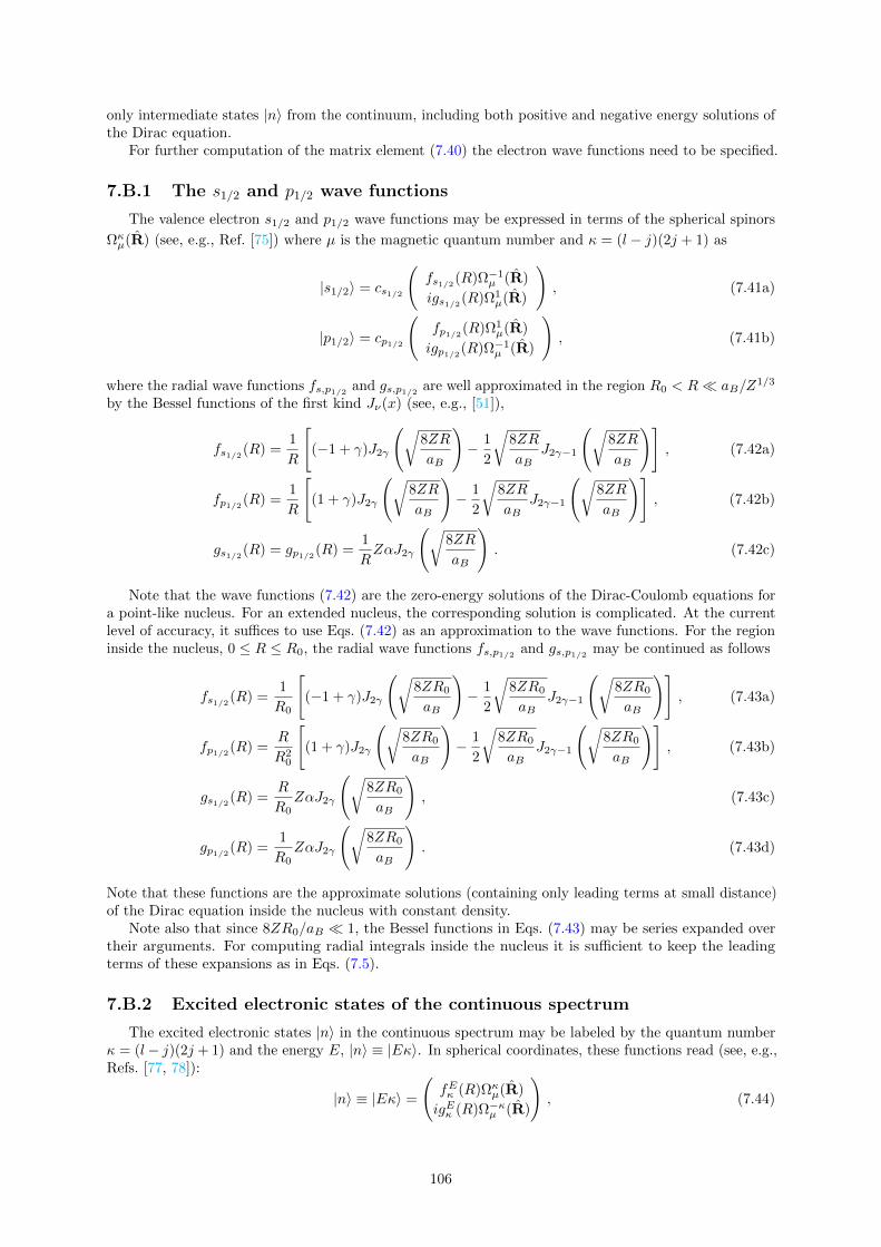
only intermediate states |n〉 from the continuum, including both positive and negative energy solutions ofthe Dirac equation.

For further computation of the matrix element (7.40) the electron wave functions need to be specified.

7.B.1 The s1/2 and p1/2 wave functions

The valence electron s1/2 and p1/2 wave functions may be expressed in terms of the spherical spinors

Ωκµ(R) (see, e.g., Ref. [75]) where µ is the magnetic quantum number and κ = (l − j)(2j + 1) as

|s1/2〉 = cs1/2

(fs1/2(R)Ω−1

µ (R)

igs1/2(R)Ω1µ(R)

), (7.41a)

|p1/2〉 = cp1/2

(fp1/2(R)Ω1

µ(R)

igp1/2(R)Ω−1µ (R)

), (7.41b)

where the radial wave functions fs,p1/2 and gs,p1/2 are well approximated in the region R0 < R aB/Z1/3

by the Bessel functions of the first kind Jν(x) (see, e.g., [51]),

fs1/2(R) =1

R

[(−1 + γ)J2γ

(√8ZR

aB

)− 1

2

√8ZR

aBJ2γ−1

(√8ZR

aB

)], (7.42a)

fp1/2(R) =1

R

[(1 + γ)J2γ

(√8ZR

aB

)− 1

2

√8ZR

aBJ2γ−1

(√8ZR

aB

)], (7.42b)

gs1/2(R) = gp1/2(R) =1

RZαJ2γ

(√8ZR

aB

). (7.42c)

Note that the wave functions (7.42) are the zero-energy solutions of the Dirac-Coulomb equations fora point-like nucleus. For an extended nucleus, the corresponding solution is complicated. At the currentlevel of accuracy, it suffices to use Eqs. (7.42) as an approximation to the wave functions. For the regioninside the nucleus, 0 ≤ R ≤ R0, the radial wave functions fs,p1/2 and gs,p1/2 may be continued as follows

fs1/2(R) =1

R0

[(−1 + γ)J2γ

(√8ZR0

aB

)− 1

2

√8ZR0

aBJ2γ−1

(√8ZR0

aB

)], (7.43a)

fp1/2(R) =R

R20

[(1 + γ)J2γ

(√8ZR0

aB

)− 1

2

√8ZR0

aBJ2γ−1

(√8ZR0

aB

)], (7.43b)

gs1/2(R) =R

R0ZαJ2γ

(√8ZR0

aB

), (7.43c)

gp1/2(R) =1

R0ZαJ2γ

(√8ZR0

aB

). (7.43d)

Note that these functions are the approximate solutions (containing only leading terms at small distance)of the Dirac equation inside the nucleus with constant density.

Note also that since 8ZR0/aB 1, the Bessel functions in Eqs. (7.43) may be series expanded overtheir arguments. For computing radial integrals inside the nucleus it is sufficient to keep the leadingterms of these expansions as in Eqs. (7.5).

7.B.2 Excited electronic states of the continuous spectrum

The excited electronic states |n〉 in the continuous spectrum may be labeled by the quantum numberκ = (l− j)(2j + 1) and the energy E, |n〉 ≡ |Eκ〉. In spherical coordinates, these functions read (see, e.g.,Refs. [77, 78]):

|n〉 ≡ |Eκ〉 =

(fEκ (R)Ωκµ(R)

igEκ (R)Ω−κµ (R)

), (7.44)

106

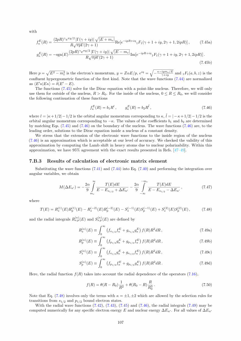
with

fEκ (R) =(2pR)γeπy/2 |Γ(γ + iy)|

√|E +me|

R√πpΓ(2γ + 1)

Re[e−ipR+iη1F1(γ + 1 + iy, 2γ + 1, 2ipR)] , (7.45a)

gEκ (R) = −sgn(E)(2pR)γeπy/2 |Γ(γ + iy)|

√|E −me|

R√πpΓ(2γ + 1)

Im[e−ipR+iη1F1(γ + 1 + iy, 2γ + 1, 2ipR)] .

(7.45b)

Here p =√E2 −m2

e is the electron’s momentum, y = ZαE/p, eiη =√−κ−iyme/Eγ+iy and 1F1(a, b, z) is the

confluent hypergeometric function of the first kind. Note that the wave functions (7.44) are normalizedas 〈E′κ|Eκ〉 = δ(E′ − E).

The functions (7.45) solve for the Dirac equation with a point-like nucleus. Therefore, we will onlyuse them for outside of the nucleus, R > R0. For the inside of the nucleus, 0 ≤ R ≤ R0, we will considerthe following continuation of these functions

fEκ (R) = b1Rl , gEκ (R) = b2R

l , (7.46)

where l = |κ+ 1/2|−1/2 is the orbital angular momentum corresponding to κ, l = |−κ+ 1/2|−1/2 is theorbital angular momentum corresponding to −κ. The values of the coefficients b1 and b2 are determinedby matching Eqs. (7.45) and (7.46) on the boundary of the nucleus. The wave functions (7.46) are, to theleading order, solutions to the Dirac equation inside a nucleus of a constant density.

We stress that the extension of the electronic wave functions to the inside region of the nucleus(7.46) is an approximation which is acceptable at our level of accuracy. We checked the validity of thisapproximation by computing the Lamb shift in heavy atoms due to nuclear polarizability. Within thisapproximation, we have 95% agreement with the exact results presented in Refs. [47–49].

7.B.3 Results of calculation of electronic matrix element

Substituting the wave functions (7.41) and (7.44) into Eq. (7.40) and performing the integration overangular variables, we obtain

M(∆En′) = −2α

9

∞∫me

T (E)dE

E − Es1/2 + ∆En′− 2α

9

−me∫−∞

T (E)dE

E − Es1/2 −∆En′, (7.47)

where

T (E) = R(1)s (E)R(1)

p (E)−R(−2)s (E)R(−2)

p (E)− S(−1)s (E)S(−1)

p (E) + S(2)s (E)S(2)

p (E) , (7.48)

and the radial integrals R(κ)s,p (E) and S

(κ)s,p (E) are defined by

R(κ)s (E) ≡

∫ ∞0

(fs1/2f

Eκ + gs1/2g

Eκ

)f(R)R2dR , (7.49a)

R(κ)p (E) ≡

∫ ∞0

(fp1/2g

Eκ + gp1/2f

Eκ

)f(R)R2dR , (7.49b)

S(κ)s (E) ≡

∫ ∞0

(fs1/2g

Eκ + gs1/2f

Eκ

)f(R)R2dR , (7.49c)

S(κ)p (E) ≡

∫ ∞0

(fp1/2f

Eκ + gp1/2g

Eκ

)f(R)R2dR . (7.49d)

Here, the radial function f(R) takes into account the radial dependence of the operators (7.16),

f(R) = θ(R−R0)1

R2+ θ(R0 −R)

R

R30

. (7.50)

Note that Eq. (7.48) involves only the terms with κ = ±1,±2 which are allowed by the selection rules fortransitions from s1/2 and p1/2 bound electron states.

With the radial wave functions (7.42), (7.43), (7.45) and (7.46), the radial integrals (7.49) may becomputed numerically for any specific electron energy E and nuclear energy ∆En′ . For all values of ∆En′

107

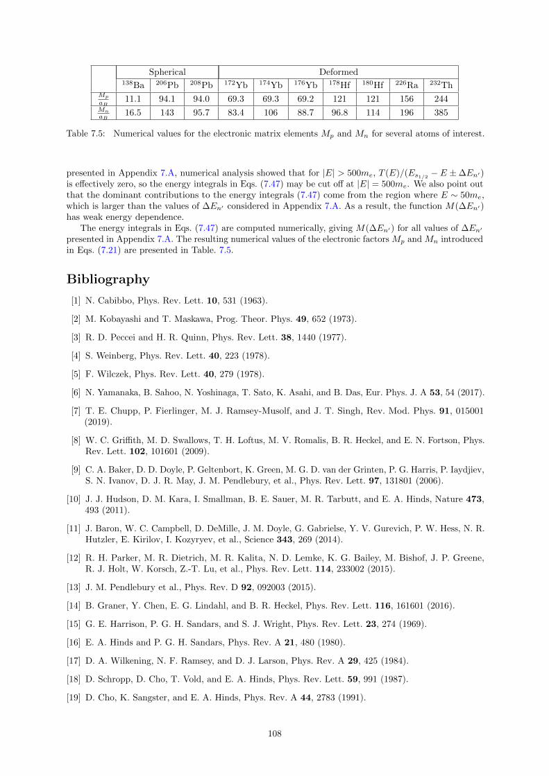
Spherical Deformed138Ba 206Pb 208Pb 172Yb 174Yb 176Yb 178Hf 180Hf 226Ra 232Th

Mp

aB11.1 94.1 94.0 69.3 69.3 69.2 121 121 156 244

Mn

aB16.5 143 95.7 83.4 106 88.7 96.8 114 196 385

Table 7.5: Numerical values for the electronic matrix elements Mp and Mn for several atoms of interest.

presented in Appendix 7.A, numerical analysis showed that for |E| > 500me, T (E)/(Es1/2 − E ±∆En′)is effectively zero, so the energy integrals in Eqs. (7.47) may be cut off at |E| = 500me. We also point outthat the dominant contributions to the energy integrals (7.47) come from the region where E ∼ 50me,which is larger than the values of ∆En′ considered in Appendix 7.A. As a result, the function M(∆En′)has weak energy dependence.

The energy integrals in Eqs. (7.47) are computed numerically, giving M(∆En′) for all values of ∆En′presented in Appendix 7.A. The resulting numerical values of the electronic factors Mp and Mn introducedin Eqs. (7.21) are presented in Table. 7.5.

Bibliography

[1] N. Cabibbo, Phys. Rev. Lett. 10, 531 (1963).

[2] M. Kobayashi and T. Maskawa, Prog. Theor. Phys. 49, 652 (1973).

[3] R. D. Peccei and H. R. Quinn, Phys. Rev. Lett. 38, 1440 (1977).

[4] S. Weinberg, Phys. Rev. Lett. 40, 223 (1978).

[5] F. Wilczek, Phys. Rev. Lett. 40, 279 (1978).

[6] N. Yamanaka, B. Sahoo, N. Yoshinaga, T. Sato, K. Asahi, and B. Das, Eur. Phys. J. A 53, 54 (2017).

[7] T. E. Chupp, P. Fierlinger, M. J. Ramsey-Musolf, and J. T. Singh, Rev. Mod. Phys. 91, 015001(2019).

[8] W. C. Griffith, M. D. Swallows, T. H. Loftus, M. V. Romalis, B. R. Heckel, and E. N. Fortson, Phys.Rev. Lett. 102, 101601 (2009).

[9] C. A. Baker, D. D. Doyle, P. Geltenbort, K. Green, M. G. D. van der Grinten, P. G. Harris, P. Iaydjiev,S. N. Ivanov, D. J. R. May, J. M. Pendlebury, et al., Phys. Rev. Lett. 97, 131801 (2006).

[10] J. J. Hudson, D. M. Kara, I. Smallman, B. E. Sauer, M. R. Tarbutt, and E. A. Hinds, Nature 473,493 (2011).

[11] J. Baron, W. C. Campbell, D. DeMille, J. M. Doyle, G. Gabrielse, Y. V. Gurevich, P. W. Hess, N. R.Hutzler, E. Kirilov, I. Kozyryev, et al., Science 343, 269 (2014).

[12] R. H. Parker, M. R. Dietrich, M. R. Kalita, N. D. Lemke, K. G. Bailey, M. Bishof, J. P. Greene,R. J. Holt, W. Korsch, Z.-T. Lu, et al., Phys. Rev. Lett. 114, 233002 (2015).

[13] J. M. Pendlebury et al., Phys. Rev. D 92, 092003 (2015).

[14] B. Graner, Y. Chen, E. G. Lindahl, and B. R. Heckel, Phys. Rev. Lett. 116, 161601 (2016).

[15] G. E. Harrison, P. G. H. Sandars, and S. J. Wright, Phys. Rev. Lett. 23, 274 (1969).

[16] E. A. Hinds and P. G. H. Sandars, Phys. Rev. A 21, 480 (1980).

[17] D. A. Wilkening, N. F. Ramsey, and D. J. Larson, Phys. Rev. A 29, 425 (1984).

[18] D. Schropp, D. Cho, T. Vold, and E. A. Hinds, Phys. Rev. Lett. 59, 991 (1987).

[19] D. Cho, K. Sangster, and E. A. Hinds, Phys. Rev. A 44, 2783 (1991).

108

[20] T. G. Vold, F. J. Raab, B. Heckel, and E. N. Fortson, Phys. Rev. Lett. 52, 2229 (1984).

[21] T. E. Chupp, R. J. Hoare, R. L. Walsworth, and B. Wu, Phys. Rev. Lett. 72, 2363 (1994).

[22] R. E. Stoner, M. A. Rosenberry, J. T. Wright, T. E. Chupp, E. R. Oteiza, and R. L. Walsworth,Phys. Rev. Lett. 77, 3971 (1996).

[23] D. Bear, T. E. Chupp, K. Cooper, S. DeDeo, M. Rosenberry, R. E. Stoner, and R. L. Walsworth,Phys. Rev. A 57, 5006 (1998).

[24] M. A. Rosenberry and T. E. Chupp, Phys. Rev. Lett. 86, 22 (2001).

[25] M. V. Romalis, W. C. Griffith, J. P. Jacobs, and E. N. Fortson, Phys. Rev. Lett. 86, 2505 (2001).

[26] M. Bishof, R. H. Parker, K. G. Bailey, J. P. Greene, R. J. Holt, M. R. Kalita, W. Korsch, N. D.Lemke, Z.-T. Lu, P. Mueller, et al., Phys. Rev. C 94, 025501 (2016).

[27] H. Loh, K. C. Cossel, M. C. Grau, K.-K. Ni, E. R. Meyer, J. L. Bohn, J. Ye, and E. A. Cornell,Science 342, 1220 (2013).

[28] S. Eckel, P. Hamilton, E. Kirilov, H. W. Smith, and D. DeMille, Phys. Rev. A 87, 052130 (2013).

[29] W. B. Cairncross, D. N. Gresh, M. Grau, K. C. Cossel, T. S. Roussy, Y. Ni, Y. Zhou, J. Ye, andE. A. Cornell, Phys. Rev. Lett. 119, 153001 (2017).

[30] P. Aggarwal, H. L. Bethlem, A. Borschevsky, M. Denis, K. Esajas, P. A. Haase, Y. Hao, S. Hoekstra,K. Jungmann, T. B. Meijknecht, et al., Eur. Phys. J. D 72, 197 (2018).

[31] V. Andreev, D. G. Ang, D. DeMille, J. M. Doyle, G. Gabrielse, J. Haefner, N. R. Hutzler, Z. Lasner,C. Meisenhelder, B. R. O’Leary, et al. (ACME), Nature 562, 355 (2018).

[32] V. Flambaum, M. Pospelov, A. Ritz, and Y. Stadnik, Phys. Rev. D 102, 035001 (2020).

[33] T. S. Roussy et al., arXiv:2006.15787 (2020).

[34] P. W. Graham and S. Rajendran, Phys. Rev. D 84, 055013 (2011).

[35] L. I. Schiff, Phys. Rev. 132, 2194 (1963).

[36] O. P. Sushkov, V. V. Flambaum, and I. B. Khriplovich, Zh. Eksp. Teor. Fiz 87, 1521 (1984).

[37] V. V. Flambaum, I. B. Khriplovich, and O. P. Sushkov, Nucl. Phys. A 449, 750 (1986).

[38] V. V. Flambaum, Phys. Lett. B 320, 211 (1994).

[39] V. A. Dzuba, V. V. Flambaum, P. G. Silvestrov, and O. P. Sushkov, Phys. Lett. A 118, 177 (1986).

[40] V. V. Flambaum, Phys. Rev. A 98, 043408 (2018).

[41] H. B. Tran Tan, V. V. Flambaum, and I. B. Samsonov, Phys. Rev. A 99, 013430 (2019).

[42] V. V. Flambaum and I. B. Samsonov, Phys. Rev. A 98, 053437 (2018).

[43] V. V. Flambaum and I. B. Samsonov, Phys. Rev. Res. 2, 023042 (2020).

[44] V. V. Flambaum, J. S. M. Ginges, and G. Mititelu, arXiv:nucl-th/0010100 (2000).

[45] V. V. Flambaum and I. B. Khriplovich, Zh. Eksp. Theor. Fiz 89, 1505 (1985).

[46] J. Bsaisou, U.-G. Meißner, A. Nogga, and A. Wirzba, Annals Phys. 359, 317 (2015).

[47] G. Plunien, B. Muller, W. Greiner, and G. Soff, Phys. Rev. A 43, 5853 (1991).

[48] K. Pachucki, D. Leibfried, and T. W. Hansch, Phys. Rev. A 48, R1 (1993).

[49] G. Plunien and G. Soff, Phys. Rev. A 51, 1119 (1995).

[50] S. G. Nilsson, Dan. Mat. Fys. Medd. 29, 1 (1955).

109

[51] I. B. Khriplovich, Parity nonconservation in atomic phenomena (Gordon and Breach SciencePublishers, 1991).

[52] P. Sarriguren, E. Moya de Guerra, and R. Nojarov, Phys. Rev. C 54, 690 (1996).

[53] T. Fleig and M. Jung, J. High Energy Phys. 2018, 12 (2018).

[54] M. Pospelov and A. Ritz, Ann. Phys. 318, 119 (2005), special Issue.

[55] R. J. Crewther, P. Di Vecchia, G. Veneziano, and E. Witten, Phys. Let. B 88, 123 (1979).

[56] W. Hockings and U. van Kolck, Phys. Lett. B 605, 273 (2005).

[57] K. Ottnad, B. Kubis, U.-G. Meissner, and F.-K. Guo, Phys. Lett. B 687, 42 (2010).

[58] F.-K. Guo and U.-G. Meissner, J. High Energy Phys. 12, 097 (2012).

[59] M. Pospelov and A. Ritz, Phys. Rev. Lett. 83, 2526 (1999).

[60] V. V. Flambaum, D. DeMille, and M. G. Kozlov, Phys. Rev. Lett. 113, 103003 (2014).

[61] M. Pospelov and A. Ritz, Phys. Rev. D 63, 073015 (2001).

[62] F. Abusaif et al., arXiv:1912.07881 (2019).

[63] J. de Vries, E. Mereghetti, and A. Walker-Loud, Phys. Rev. C 92, 045201 (2015).

[64] J. Bsaisou, J. de Vries, C. Hanhart, S. Liebig, U.-G. Meißner, D. Minossi, A. Nogga, and A. Wirzba,J. High Energy Phys. 2015, 104 (2015).

[65] J. de Vries and U.-G. Meißner, Int. J. Mod. Phys. E 25, 1641008 (2016).

[66] J. Bsaisou, C. Hanhart, S. Liebig, U.-G. Meißner, A. Nogga, and A. Wirzba, Eur. Phys. J. A 49, 1(2013).

[67] C. Abel, S. Afach, N. J. Ayres, C. A. Baker, G. Ban, G. Bison, K. Bodek, V. Bondar, M. Burghoff,E. Chanel, et al., Phys. Rev. Lett. 124, 081803 (2020).

[68] V. V. Flambaum and V. A. Dzuba, Phys. Rev. A 101, 042504 (2020).

[69] B. K. Sahoo, Phys. Rev. D 95, 013002 (2017).

[70] N. Sachdeva, I. Fan, E. Babcock, M. Burghoff, T. E. Chupp, S. Degenkolb, P. Fierlinger, S. Haude,E. Kraegeloh, W. Kilian, et al., Phys. Rev. Lett. 123, 143003 (2019).

[71] F. Allmendinger, I. Engin, W. Heil, S. Karpuk, H.-J. Krause, B. Niederlander, A. Offenhausser,M. Repetto, U. Schmidt, and S. Zimmer, Phys. Rev. A 100, 022505 (2019).

[72] M. Tanabashi et al. (Particle Data Group), Phys. Rev. D 98, 030001 (2018).

[73] S. Ban, J. Dobaczewski, J. Engel, and A. Shukla, Phys. Rev. C 82, 015501 (2010).

[74] H. Loh, K. C. Cossel, M. C. Grau, K.-K. Ni, E. R. Meyer, J. L. Bohn, J. Ye, and E. A. Cornell,Science 342, 1220 (2013).

[75] R. Szmytkowski, J. Math. Chem. 42, 397 (2007).

[76] A. Bohr and B. R. Mottelson, Nuclear Structure, vol. 2 (World Scientific, Singapore, 1998).

[77] V. B. Berestetskii, E. M. Lifshitz, and L. P. Pitaevskii, Quantum electrodynamics, vol. 4 (Butterworth-Heinemann, 1982).

[78] W. Greiner, Relativistic quantum mechanics: Wave Equations, vol. 2 (Springer, 2000).

110

Chapter 8

Effects of CP -violating internucleoninteractions in paramagneticmolecules

8.1 Overview

In chapter 7, I showed that nucleon EDMs can induce atomic EDM via the combined electric andmagnetic electron-nucleon interaction. In this chapter, I demonstrate that CP -odd internucleon forcescan have similar effects: when coupled with electron-nucleon electric and magnetic interaction, theyinduce measurable atomic EDMs.

As a result of my research, I have published the following paper:

1. V. V. Flambaum, I. B. Samsonov and H. B. Tran TanEffects CP-violating internucleon interactions in paramagnetic moleculesPhys. Rev. D 102, 115036 (2020), DOI: 10.1103/PhysRevD.102.115036, arXiv:2009.07992.

8.2 Abstract

We demonstrate that electron electric dipole moment (eEDM) experiments with molecules in para-magnetic state are sensitive to P, T -violating nuclear forces and other CP -violating parameters in thehadronic sector. These experiments, in particular, measure the coupling constant CSP of the CP -oddcontact semileptonic interaction. We establish relations between CSP and different CP -violating hadronicparameters including strength constants of the CP -odd nuclear potentials, CP -odd pion-nucleon interac-tions, quark-chromo EDM and QCD vacuum angle. These relations allow us to find limits on variousCP -odd hadronic parameters.

8.3 Introduction

The existence of non-vanishing electric dipole moments (EDMs) of elementary particles was conjecturednearly seventy years ago [1–4], but they have not been observed so far. Their discovery would be acrucial step in the study of charge and parity (CP ) violations. On the one hand, the Standard Modelof elementary particles predicts non-vanishing values for the EDMs of the electron and nucleons, butthese values are so minuscule that they are practically unobservable in current experiments. On the otherhand, it is known that the CP -violation is needed to explain the apparent matter-antimatter asymmetryin the universe [5]. It is therefore an important challenge for experimental physics to measure the EDMsof elementary particles as well as EDMs of composite objects such as nucleons, nuclei and atoms.

In the last decade or so, tremendous progress has been achieved in the experiments with paramageticmolecules which measure the electron EDM through specific energy level shifts [6, 7] (see also Refs. [8, 9]for reviews). As was demonstrated in the recent works [10, 11], these experiments are also sensitive to theCP -violating interactions in the hadronic sector, which originate, in particular, from the nucleon EDMs.The aim of the current work is to extend the results of the papers [10, 11] and to study the sensitivity ofparamagnetic EDM experiments to P, T -violating nuclear forces.

111

It is a well-known fact that the CP -violating effects are significantly enhanced in heavy atoms [12].In this paper, we consider a single-particle nuclear model in which the open-shell nucleon interacts with aheavy nuclear core through a nuclear potential U(r). The P, T -violating nuclear forces are taken intoaccount by the phenomenological interaction Hamiltonian Hodd = ξσ · ∇U(r), where σ/2 is the nucleonspin operator and ξ is the coupling constant of dimension of length. This coupling constant will bedenoted by ξp for proton and ξn for neutron. The authors of Ref. [13] demonstrated that the leadingcontributions to this interaction arise due to π meson exchange between the open-shell nucleon andthe nuclear core. In general, however, this interaction may arise due to the CP -violating πNN , ηNN ,three-pion and four-nucleon interactions. The last two interactions were considered, in particular, inRef. [14].

In this paper, we will focus on the contributions to the atomic EDM arising due to the P, T -oddnuclear force with the Hamiltonian Hodd regardless of the underlying fundamental interaction. Inprinciple, experimental limits on the phenomenological parameters ξp,n may be converted into limits onthe parameters of more fundamental hadronic interactions. We stress that the interaction Hodd consideredin this work is an independent source of CP violating effects, separate from the contributions due tonucleon EDMs considered in Refs. [10, 11].

The most stringent experimental constraint on the electron EDM was obtained by the ACMEcollaboration [6] which measured specific energy level shifts in the 232ThO molecule. Based on theoreticalcalculations [15, 16], this experiment also placed a limit on the CP -odd electron-nucleon interactioncoupling constant (90% C.L.),

|CSP |Th < 7.3× 10−10 . (8.1)

In a heavy, spinless nucleus with Z protons and N = A − Z neutrons this coupling constant is alinear combination of independent electron couplings to protons (CpSP ) and neutrons (CnSP ), CSP =CpSPZ/A+CnSPN/A. The latter two coupling constants correspond to the following CP -odd semileptonicoperators

L =iGF√

2CpSP eγ5e pp+

iGF√2CnSP eγ5e nn , (8.2)

where GF is the Fermi coupling constant, e, p and n are respectively the electron, proton and neutronfields. Note that the subscript ‘SP ’ denotes the nucleon-scalar and electron pseudoscalar two-fermionbilinears.1

Our goal is to establish the leading-order relation between the coupling constant CSP and theparameters of the P, T -odd internucleon interaction ξp and ξn, CSP = CSP (ξp, ξn). This will allow usto find limits on these couplings originating from the experimental constraint (8.1). Then, using knownrelations between the constants ξp, ξn and more fundamental CP -violating hadronic parameters, we will

establish leading-order relation between CSP and CP -odd pion-nucleon couplings g(0,1,2)πNN , quark-chromo

EDMs du,d and QCD vacuum angle θ.Note that this problem involves the third order perturbation theory in the nuclear part and second

order in the electron-nucleus interaction. To get through these complications we have to make someapproximations in the nuclear part of the problem where we perform the calculations analytically. Whileall these approximations are common and justifiable, we cannot pretend that the accuracy of our results isbetter than a factor of two [12, 13, 17]. However, this accuracy is comparable to that in other calculationsof the hadronic contributions to atomic EDM where the limits on the CP -violating parameters are oftenpresented on the logarithmic scale. For instance, current limit on QCD vacuum angle reads |θ| < 10−10,see, e.g., reviews [8, 9] and updated limits presented in Ref. [18].

The rest of the paper is organized as follows. In Sect. 8.4, we present an estimate for the atomic EDMarising from the CP -odd nuclear forces. In Sect. 8.5, we compare this contribution to the atomic EDMwith that of the contact electron-nucleon interaction and the nucleon permanent EDMs and find relationsbetween the constant CSP and CP -violating hadronic parameters. In Sect. 8.6 we give a summary of ourresults and provide some comments on assumptions and precision. Technical details of calculations ofelectronic and nuclear matrix elements are collected in appendices.

Throughout this paper we use natural units with c = ~ = 1.

1In general, there are also nucleon-pseudoscalar and electron-scalar (‘PS’) as well as tensor-tensor (‘TT ’) CP -violatingsemileptonic interactions. These interactions play subleading role in atoms with spinless nuclei and, therefore, they will beignored in this paper.

112

8.4 Contributions to the atomic EDM from P, T -odd nuclearforces

In this section, we determine the contributions to the atomic EDM arising due to nuclear P, T -oddinteractions. In Sect. 8.4.1 we start with a review of the P, T -perturbed nuclear wave functions, whichwere found in Ref. [13]. These wave functions will be used in Sect. 8.4.2 for the computation of thenuclear matrix elements contributing to the atomic EDM.

8.4.1 Nuclear wave functions perturbed by P, T -odd nuclear interactions

The nucleons in a nucleus can exhibit different P, T -odd interactions originating both from theStandard Model and beyond. Independently of their nature, in the non-relativistic limit, these short-rangeinteractions may be taken into account by the following phenomenological single-particle Hamiltonian [13]

Hodd =GF√

2

η

2mpσ · ∇ρ(r) , (8.3)

where σ/2 is the spin of the open-shell non-relativistic nucleon, ρ(r) is the density of the nuclear core, ηis the effective coupling constant and mp is the proton mass.

In a heavy nucleus, the nuclear core creates an effective nuclear potential U(r) in which the open-shellnucleon moves. In the short-range approximation, this potential is proportional to the density of thenuclear core, ρ(r) = U(r)ρ(0)/U(0). Taking this into account, the Hamiltonian (8.3) may be representedas

Hodd = ξσ · ∇U(r) , (8.4)

where [13]

ξ = ηGF

2√

2mp

ρ(0)

U(0)≈ −2× 10−21η · cm . (8.5)

The total potential for the open-shell nucleon is thus given by

U = U +Hodd = U + ξσ · ∇U ≈ U(r + ξσ) . (8.6)

Now let ψn′(r) be unperturbed single-nucleon wave function labeled by some quantum numbers n′.This function is supposed to solve for the Schrodinger equation with the potential U(r). Equation (8.6)suggests that the wave function perturbed by the P, T -odd interaction (8.3) may be represented as

ψn′(r) = ψn′(r + ξσ) ≈ (1 + ξσ · ∇)ψn′(r) , (8.7)

or, more generally, generalizing to all nucleons

ψn′(r1, ..., rA) =

(1 +

A∑τ=1

ξτστ · ∇τ

)ψn′(r1, ..., rA) , (8.8)

where ψn′(r1, ..., rA) and ψn′(r1, ..., rA) are multi-palrticle nuclear wave functions. Note that the constantsξτ are different for proton (ξτ = ξp) and neutron (ξτ = ξn).

According to Eq. (8.8), the matrix elements of an operator O may be written up to the first order incoupling constant ξ as

〈m′|O|n′〉 = 〈m′|O|n′〉 −A∑τ=1

ξτ 〈m′|[στ · ∇τ ,O]|n′〉 , (8.9)

where |n′〉 and |n′〉 are the kets corresponding to the wave functions ψn′(r1, ..., rA) and ψn′(r1, ..., rA),respectively.

The P, T -perturbed wave functions (8.8) were found in Ref. [13]. In the next subsection we will usethese wave functions to compute the nuclear matrix elements contributing to the atomic EDM.

113

8.4.2 Electron-nucleon interaction Hamiltonian

Let us consider a valence electron of charge −e and position vector R interacting with nucleons ofcharge qτ located at the point rτ . The interaction Hamiltonian considered in this paper is a combinationof the electric (q) and magnetic (µ) terms,

Hint = −A∑τ=1

(Hqτ +Hµ

τ ) , (8.10a)

Hqτ =

eqτ|R− rτ |

, (8.10b)

Hµτ =

eµτ · [(R− rτ )×α]

|R− rτ |3, (8.10c)

whereµτ = µ0(glτ lτ + gsτsτ ) (8.11)

is the nucleon’s magnetic moment operator, µ0 is the nuclear magneton, glτ and gsτ are the orbital andspin g-factors of the nucleon. Note that sτ = στ/2 is the nucleon spin operator while α = ( 0 σ

σ 0 ) are theDirac matrices acting on electron’s states. We point out that since we consider spinless nuclei in thispaper, the interaction (7.7a) does not arise if the nucleus is treated as a pointlike object.

The interaction Hamiltonian (8.10) as a function of R and rτ may be expanded into a multipole series.In particular, the leading terms in the expansion of the electric interaction Hamiltonian (8.10b) are

Hqτ = eqτ

(1

R+

R · rτR3

)θ(R− rτ ) + eqτ

(1

r+

R · rτr3τ

)θ(rτ −R) + . . . , (8.12)

where the ellipsis stand for terms with higher multipolarity. In this expansion, the term θ(R− rτ )/R+θ(rτ −R)/rτ , after averaging with the nuclear charge density ρ(r), gives rise to the Coulomb interactionof the electron with the extended nucleus. This interaction is assumed to have already been taken intoaccount by the unperturbed electronic wave functions.

The term (R · rτ )[θ(R− rτ )/R3 + θ(rτ −R)/r3τ ] in Eq. (8.12) is the leading dipole one on which we

will focus our attention2. Evidently, at a distance from the nucleus, this term falls off as 1/R2. To findthe effective electron-nucleon interaction Hamiltonian inside the nucleus, one needs to average this termover the normalized nuclear density, which, in the leading approximation, may be taken as constant insidethe sphere of radius R0 and vanishing outside, ρ(r) = 3θ(R0 − r)/R3

0. Since ρ(r) is only needed for thecalculation of electronic matrix elements, where dominant contribution comes from outside the nucleus,this approximation does not greatly affect our results. Indeed, a computation which uses a more realisticWoods-Saxon model for the nuclear density only gives a difference of about 3%. The constant densityapproximation has the advantage of giving analytical form for the regularized potentials. In fact, it wasused in the calculation of Lamb shift due to nuclear polarizability [19–22] and hyperfine structure whichgave perfect agreement with experiments.

Using this prescription, one may obtain the following continuation of the 1/R2 function to smalldistance

f(R) ≡∫ ∞

0

ρ(r)

[1

R2θ(R− r) +

1

r2θ(r −R)

]r2dr =

1

R2θ(R−R0) +

3R0 − 2R

R30

θ(R0 −R) , (8.13)

with which the regularized dipole interaction operator (8.12) takes the form

Hqτ ≡ eqτ (R · rτ )f(R) , (8.14)

where R ≡ R/R.The magnetic interaction operator (8.10c) also behaves as 1/R2 at large distances from the nucleus

and may also be extended to the short-distance region inside the nucleus according to the prescription(8.13),

Hµτ ≡ eµτ · (R×α)f(R) . (8.15)

2This expansion is needed to describe the interaction between the nucleus and the electron. The contribution inside thenucleus is relatively small, the dominant contribution comes from the region outside the nucleus. This justifies the use ofthe dipole term for the electronic variables.

114

Thus, the dipole part of the interaction (8.10a) which is regularized at short distances reads

Hint = −A∑τ=1

(Hqτ + Hµ

τ ) , (8.16)

with Hqτ and Hµ

τ given by Eqs. (8.14) and (8.15).According to Eq. (8.9), to take into account the P, T -perturbed nuclear wave functions one has to

consider the commutators of the operator στ · ∇τ with the interaction Hamiltonians (8.14) and (8.15),

[στ · ∇τ , Hqτ ] = eqτ (στ · R)f(R) , (8.17a)

[στ · ∇τ , Hµτ ] = ieµ0(gsτ − glτ )f(R)(R×α) · (στ ×∇τ ) . (8.17b)

In deriving Eq. (8.17b) we have applied the following commutator identities: [σi, σj ] = 2iεijkσk and[∇i, lj ] = iεijk∇k.

8.4.3 Atomic EDM due to P, T -odd nuclear forces

The unperturbed atomic states will be denoted by |nn′〉 = |n〉|n′〉, where |n〉 and |n′〉 are electronicand nuclear states, respectively. In what follows, the nuclear quantum numbers will be distinguishedfrom the electronic ones with the apostrophe. As in Sect. 8.4, the P, T -perturbed nuclear wave functions(8.8) are denoted as |n′〉. Electronic and nuclear ground states are denoted as |0〉 and |0′〉 (or |0′〉 forunperturbed state), respectively.

The atomic EDM arising from the mixed interaction Hint may be calculated in perturbation theory.The first-order contribution to the atomic EDM vanishes for spinless nuclei which we consider in thispaper, ∑

n 6=0

〈0| − eR|n〉〈n0′|Hint|0′0〉E0 − En

= 0 . (8.18)

Indeed, it may be shown that 〈0′|Hint|0′〉 ∝ 〈0′|s|0′〉=0, where s ≡∑Aτ=1 sτ is the nuclear spin operator.

The leading non-vanishing contributions to the atomic EDM thus arise in the second-order perturbationtheory,

d = 2∑

m6=0,nn′ 6=00′

〈0| − eR |m〉 〈m0′| Hint |n′n〉 〈nn′| Hint |0′0〉(Em − E0) [En − E0 + sgn(En)(En′ − E0′)]

+∑

m 6=0,nn′ 6=00′

〈00′|Hint|n′n〉〈n| − eR|m〉〈mn′|Hint|0′0〉[En − E0 + sgn(En)(En′ − E0′)][Em − E0 + sgn(Em)(En′ − E0′)]

,

(8.19)

where the sgn(En) in the denominators is needed to correctly account for the negative energy electronicstates. Indeed, the negative energy electronic states contribute with opposite sign of the nuclear energybecause they may be viewed as blocking contributions which prevent the valence electron from directlytransitioning into such states which are supposed to be completely occupied in the Dirac sea picture.

The term in the second line in Eq. (8.19) may be neglected in comparison with the other one because itis suppressed by higher power of nuclear energy in the denominator. Moreover, we assume that the leadingcontributions to the atomic EDM arise from the matrix elements with |0〉 = |s1/2〉 and |m〉 = |p1/2〉electronic states because these wave functions are significantly enhanced in the vicinity of a heavy nucleus.Taking this into account, Eq. (8.19) may be cast in the form

d ≈ 2〈s1/2|eR|p1/2〉〈p1/2|Heff |s1/2〉

Ep1/2 − Es1/2, (8.20)

where we have introduced the effective interaction Hamiltonian

Heff ≡∑

nn′ 6=00′

|m〉〈m0′|Hint|n′n〉〈nn′|Hint|0′0〉〈0|∆En + sgn(En)∆En′

. (8.21)

Here ∆En = En−E0 and ∆En′ = En′ −E0′ . Our goal is to calculate the matrix element 〈p1/2|Heff |s1/2〉which is responsible for the leading-order contributions to the atomic EDM.

115

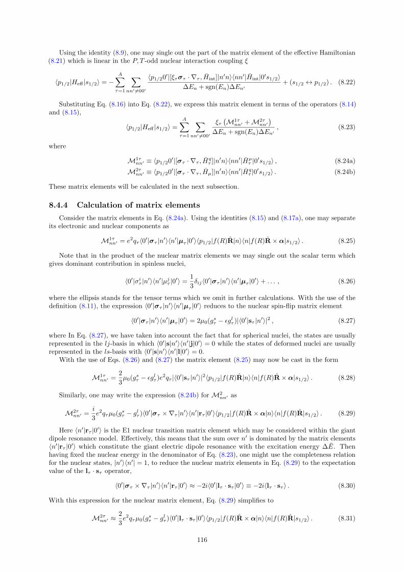
Using the identity (8.9), one may single out the part of the matrix element of the effective Hamiltonian(8.21) which is linear in the P, T -odd nuclear interaction coupling ξ

〈p1/2|Heff |s1/2〉 = −A∑τ=1

∑nn′ 6=00′

〈p1/20′|[ξτστ · ∇τ , Hint]|n′n〉〈nn′|Hint|0′s1/2〉∆En + sgn(En)∆En′

+ (s1/2 ↔ p1/2) . (8.22)

Substituting Eq. (8.16) into Eq. (8.22), we express this matrix element in terms of the operators (8.14)and (8.15),

〈p1/2|Heff |s1/2〉 =

A∑τ=1

∑nn′ 6=00′

ξτ(M1τ

nn′ +M2τnn′

)∆En + sgn(En)∆En′

, (8.23)

where

M1τnn′ ≡ 〈p1/20′|[στ · ∇τ , Hq

τ ]|n′n〉〈nn′|Hµτ |0′s1/2〉 , (8.24a)

M2τnn′ ≡ 〈p1/20′|[στ · ∇τ , Hµ]|n′n〉〈nn′|Hq

τ |0′s1/2〉 . (8.24b)

These matrix elements will be calculated in the next subsection.

8.4.4 Calculation of matrix elements

Consider the matrix elements in Eq. (8.24a). Using the identities (8.15) and (8.17a), one may separateits electronic and nuclear components as

M1τnn′ = e2qτ 〈0′|στ |n′〉〈n′|µτ |0′〉〈p1/2|f(R)R|n〉〈n|f(R)R×α|s1/2〉 . (8.25)

Note that in the product of the nuclear matrix elements we may single out the scalar term whichgives dominant contribution in spinless nuclei,

〈0′|σiτ |n′〉〈n′|µjτ |0′〉 =1

3δij〈0′|στ |n′〉〈n′|µτ |0′〉+ . . . , (8.26)

where the ellipsis stands for the tensor terms which we omit in further calculations. With the use of thedefinition (8.11), the expression 〈0′|στ |n′〉〈n′|µτ |0′〉 reduces to the nuclear spin-flip matrix element

〈0′|στ |n′〉〈n′|µτ |0′〉 = 2µ0(gsτ − εglτ )|〈0′|sτ |n′〉|2 , (8.27)

where In Eq. (8.27), we have taken into account the fact that for spherical nuclei, the states are usuallyrepresented in the lj-basis in which 〈0′|s|n′〉〈n′|j|0′〉 = 0 while the states of deformed nuclei are usuallyrepresented in the ls-basis with 〈0′|s|n′〉〈n′|l|0′〉 = 0.

With the use of Eqs. (8.26) and (8.27) the matrix element (8.25) may now be cast in the form

M1τnn′ =

2

3µ0(gsτ − εglτ )e2qτ |〈0′|sτ |n′〉|2〈p1/2|f(R)R|n〉〈n|f(R)R×α|s1/2〉 . (8.28)

Similarly, one may write the expression (8.24b) for M2nn′ as

M2τnn′ =

i

3e2qτµ0(gsτ − glτ )〈0′|στ ×∇τ |n′〉〈n′|rτ |0′〉〈p1/2|f(R)R×α|n〉〈n|f(R)R|s1/2〉 . (8.29)

Here 〈n′|rτ |0′〉 is the E1 nuclear transition matrix element which may be considered within the giantdipole resonance model. Effectively, this means that the sum over n′ is dominated by the matrix elements〈n′|rτ |0′〉 which constitute the giant electric dipole resonance with the excitation energy ∆E. Thenhaving fixed the nuclear energy in the denominator of Eq. (8.23), one might use the completeness relationfor the nuclear states, |n′〉〈n′| = 1, to reduce the nuclear matrix elements in Eq. (8.29) to the expectationvalue of the lτ · sτ operator,

〈0′|στ ×∇τ |n′〉〈n′|rτ |0′〉 ≈ −2i〈0′|lτ · sτ |0′〉 ≡ −2i〈lτ · sτ 〉 . (8.30)

With this expression for the nuclear matrix element, Eq. (8.29) simplifies to

M2τnn′ ≈

2

3e2qτµ0(gsτ − glτ )〈0′|lτ · sτ |0′〉〈p1/2|f(R)R×α|n〉〈n|f(R)R|s1/2〉 . (8.31)

116

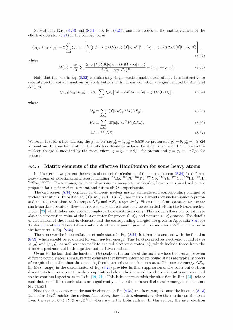
Substituting Eqs. (8.28) and (8.31) into Eq. (8.23), one may represent the matrix element of theeffective operator (8.21) in the compact form

〈p1/2|Heff |s1/2〉 = 2

A∑τ=1

ξτqτµ0

[∑n′

(gsτ − εglτ )M(En′)|〈0′|sτ |n′〉|2 + (gsτ − glτ )M(∆E)〈0′|lτ · sτ |0′〉

],

(8.32)where

M(E) ≡ e2

3

∑n

〈p1/2|f(R)R|n〉〈n|f(R)R×α|s1/2〉∆En + sgn(En)E

+ (s1/2 ↔ p1/2) . (8.33)

Note that the sum in Eq. (8.32) contains only single-particle nucleon excitations. It is instructive toseparate proton (p) and neutron (n) contributions with nuclear excitation energies denoted by ∆Ep and∆En as

〈p1/2|Heff |s1/2〉 = 2µ0

∑i=p,n

ξiqi[(gsi − εgli)Mi + (gsi − gli)M〈l · s〉i

], (8.34)

where

Mp ≡∑∆Ep

|〈0′|s|n′〉p|2M(∆Ep) , (8.35)

Mn ≡∑∆En

|〈0′|s|n′〉n|2M(∆En) , (8.36)

M ≡M(∆E) . (8.37)

We recall that for a free nucleon, the g-factors are glp = 1, gsp = 5.586 for proton and gln = 0, gsn = −3.826for neutron. In a nuclear medium, the g-factors should be reduced by about a factor of 0.7. The effectivenucleon charge is modified by the recoil effect: q = qp ≡ eN/A for proton and q = qn ≡ −eZ/A forneutron.

8.4.5 Matrix elements of the effective Hamiltonian for some heavy atoms

In this section, we present the results of numerical calculation of the matrix element (8.34) for differentheavy atoms of experimental interest including 138Ba, 206Pb, 208Pb, 172Yb, 174Yb, 176Yb, 178Hf, 180Hf,226Ra, 232Th. These atoms, as parts of various paramagnetic molecules, have been considered or areproposed for consideration in recent and future eEDM experiments.

The expression (8.34) depends on different nuclear matrix elements and corresponding energies ofnuclear transitions. In particular, 〈0′|s|n′〉p and 〈0′|s|n′〉n are matrix elements for nuclear spin-flip protonand neutron transitions with energies ∆Ep and ∆En, respectively. Since the nuclear operators we use aresingle-particle operators, these matrix elements and energies may be estimated within the Nilsson nuclearmodel [23] which takes into account single-particle excitations only. This model allows one to estimatealso the expectation value of the l · s operator for proton 〈l · s〉p and neutron 〈l · s〉n states. The detailsof calculation of these matrix elements and the corresponding energies are given in Appendix 8.A, seeTables 8.5 and 8.6. These tables contain also the energies of giant dipole resonance ∆E which enter inthe last term in Eq. (8.34).

The sum over the intermediate electronic states in Eq. (8.34) is taken into account with the function(8.33) which should be evaluated for each nuclear energy. This function involves electronic bound states|s1/2〉 and |p1/2〉, as well as intermediate excited electronic states |n〉, which include those from thediscrete spectrum and both negative and positive continua.

Owing to the fact that the function f(R) peaks at the surface of the nucleus where the overlap betweendifferent bound states is small, matrix elements that involve intermediate bound states are typically ordersof magnitude smaller than those coming from intermediate continuum states. The nuclear energy ∆En′

(in MeV range) in the denominator of Eq. (8.23) provides further suppression of the contribution fromdiscrete states. As a result, in the computation below, the intermediate electronic states are restrictedto the continual spectra as in Refs. [19, 21]. This is in contrast with the situation in Ref. [24], wherecontributions of the discrete states are significantly enhanced due to small electronic energy denominators(eV range).

Note that the operators in the matrix elements in Eq. (8.34) are short-range because the function (8.13)falls off as 1/R2 outside the nucleus. Therefore, these matrix elements receive their main contributionsfrom the region 0 < R aB/Z

1/3, where aB is the Bohr radius. In this region, the inter-electron

117

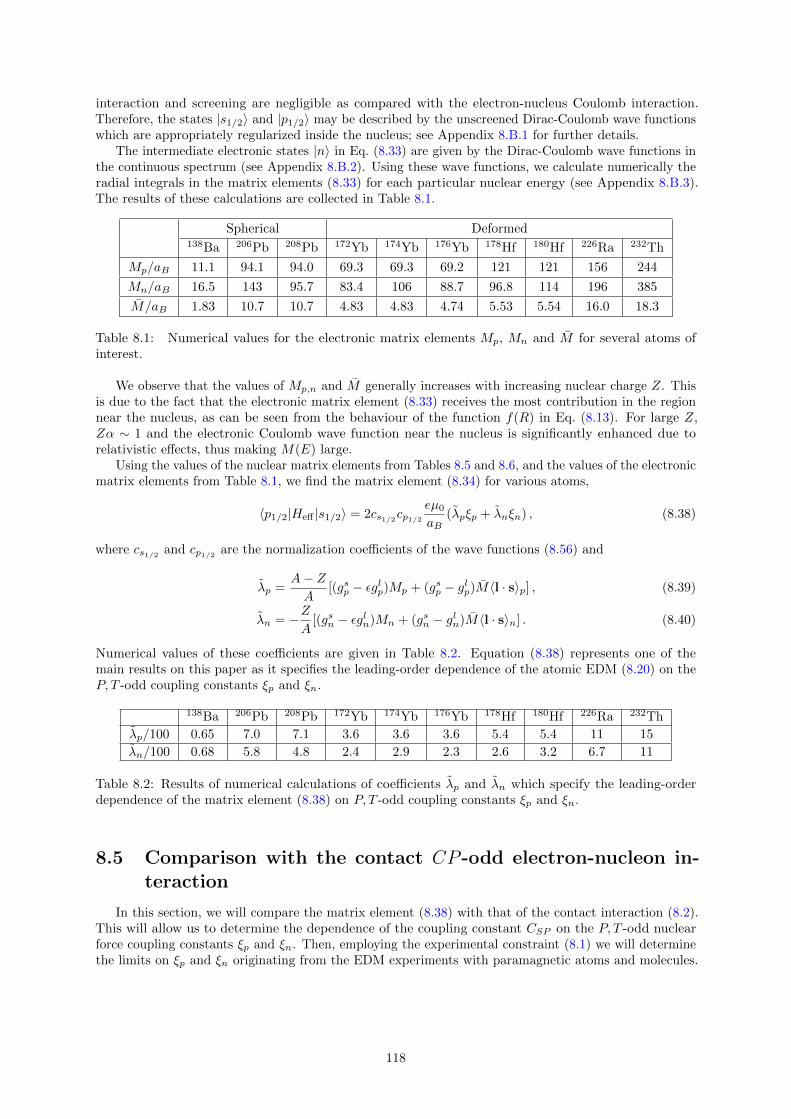
interaction and screening are negligible as compared with the electron-nucleus Coulomb interaction.Therefore, the states |s1/2〉 and |p1/2〉 may be described by the unscreened Dirac-Coulomb wave functionswhich are appropriately regularized inside the nucleus; see Appendix 8.B.1 for further details.

The intermediate electronic states |n〉 in Eq. (8.33) are given by the Dirac-Coulomb wave functions inthe continuous spectrum (see Appendix 8.B.2). Using these wave functions, we calculate numerically theradial integrals in the matrix elements (8.33) for each particular nuclear energy (see Appendix 8.B.3).The results of these calculations are collected in Table 8.1.

Spherical Deformed138Ba 206Pb 208Pb 172Yb 174Yb 176Yb 178Hf 180Hf 226Ra 232Th

Mp/aB 11.1 94.1 94.0 69.3 69.3 69.2 121 121 156 244

Mn/aB 16.5 143 95.7 83.4 106 88.7 96.8 114 196 385

M/aB 1.83 10.7 10.7 4.83 4.83 4.74 5.53 5.54 16.0 18.3

Table 8.1: Numerical values for the electronic matrix elements Mp, Mn and M for several atoms ofinterest.

We observe that the values of Mp,n and M generally increases with increasing nuclear charge Z. Thisis due to the fact that the electronic matrix element (8.33) receives the most contribution in the regionnear the nucleus, as can be seen from the behaviour of the function f(R) in Eq. (8.13). For large Z,Zα ∼ 1 and the electronic Coulomb wave function near the nucleus is significantly enhanced due torelativistic effects, thus making M(E) large.

Using the values of the nuclear matrix elements from Tables 8.5 and 8.6, and the values of the electronicmatrix elements from Table 8.1, we find the matrix element (8.34) for various atoms,

〈p1/2|Heff |s1/2〉 = 2cs1/2cp1/2eµ0

aB(λpξp + λnξn) , (8.38)

where cs1/2 and cp1/2 are the normalization coefficients of the wave functions (8.56) and

λp =A− ZA

[(gsp − εglp)Mp + (gsp − glp)M〈l · s〉p] , (8.39)

λn = −ZA

[(gsn − εgln)Mn + (gsn − gln)M〈l · s〉n] . (8.40)

Numerical values of these coefficients are given in Table 8.2. Equation (8.38) represents one of themain results on this paper as it specifies the leading-order dependence of the atomic EDM (8.20) on theP, T -odd coupling constants ξp and ξn.

138Ba 206Pb 208Pb 172Yb 174Yb 176Yb 178Hf 180Hf 226Ra 232Th

λp/100 0.65 7.0 7.1 3.6 3.6 3.6 5.4 5.4 11 15

λn/100 0.68 5.8 4.8 2.4 2.9 2.3 2.6 3.2 6.7 11

Table 8.2: Results of numerical calculations of coefficients λp and λn which specify the leading-orderdependence of the matrix element (8.38) on P, T -odd coupling constants ξp and ξn.

8.5 Comparison with the contact CP -odd electron-nucleon in-teraction

In this section, we will compare the matrix element (8.38) with that of the contact interaction (8.2).This will allow us to determine the dependence of the coupling constant CSP on the P, T -odd nuclearforce coupling constants ξp and ξn. Then, employing the experimental constraint (8.1) we will determinethe limits on ξp and ξn originating from the EDM experiments with paramagnetic atoms and molecules.

118

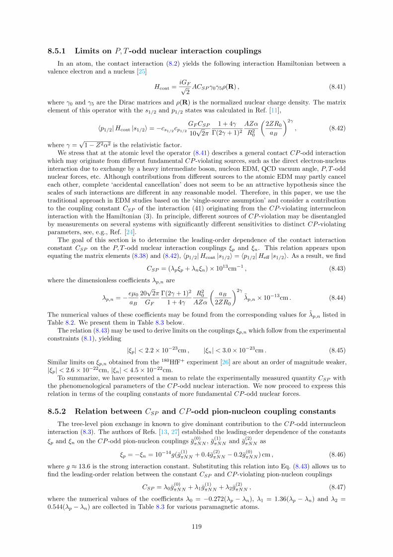
8.5.1 Limits on P, T -odd nuclear interaction couplings

In an atom, the contact interaction (8.2) yields the following interaction Hamiltonian between avalence electron and a nucleus [25]

Hcont =iGF√

2ACSP γ0γ5ρ(R) , (8.41)

where γ0 and γ5 are the Dirac matrices and ρ(R) is the normalized nuclear charge density. The matrixelement of this operator with the s1/2 and p1/2 states was calculated in Ref. [11],

〈p1/2|Hcont |s1/2〉 = −cs1/2cp1/2GFCSP

10√

2π

1 + 4γ

Γ(2γ + 1)2

AZα

R20

(2ZR0

aB

)2γ

, (8.42)

where γ =√

1− Z2α2 is the relativistic factor.We stress that at the atomic level the operator (8.41) describes a general contact CP -odd interaction

which may originate from different fundamental CP -violating sources, such as the direct electron-nucleusinteraction due to exchange by a heavy intermediate boson, nucleon EDM, QCD vacuum angle, P, T -oddnuclear forces, etc. Although contributions from different sources to the atomic EDM may partly canceleach other, complete ‘accidental cancellation’ does not seem to be an attractive hypothesis since thescales of such interactions are different in any reasonable model. Therefore, in this paper, we use thetraditional approach in EDM studies based on the ‘single-source assumption’ and consider a contributionto the coupling constant CSP of the interaction (41) originating from the CP -violating internucleoninteraction with the Hamiltonian (3). In principle, different sources of CP -violation may be disentangledby measurements on several systems with significantly different sensitivities to distinct CP -violatingparameters, see, e.g., Ref. [24].

The goal of this section is to determine the leading-order dependence of the contact interactionconstant CSP on the P, T -odd nuclear interaction couplings ξp and ξn. This relation appears uponequating the matrix elements (8.38) and (8.42), 〈p1/2|Hcont |s1/2〉 = 〈p1/2|Heff |s1/2〉. As a result, we find

CSP = (λpξp + λnξn)× 1013cm−1 , (8.43)

where the dimensionless coefficients λp,n are

λp,n = −eµ0

aB

20√

2π

GF

Γ(2γ + 1)2

1 + 4γ

R20

AZα

(aB

2ZR0

)2γ

λp,n × 10−13cm . (8.44)

The numerical values of these coefficients may be found from the corresponding values for λp,n listed inTable 8.2. We present them in Table 8.3 below.

The relation (8.43) may be used to derive limits on the couplings ξp,n which follow from the experimentalconstraints (8.1), yielding

|ξp| < 2.2× 10−23cm , |ξn| < 3.0× 10−23cm . (8.45)

Similar limits on ξp,n obtained from the 180HfF+ experiment [26] are about an order of magnitude weaker,|ξp| < 2.6× 10−22cm, |ξn| < 4.5× 10−22cm.

To summarize, we have presented a mean to relate the experimentally measured quantity CSP withthe phenomenological parameters of the CP -odd nuclear interaction. We now proceed to express thisrelation in terms of the coupling constants of more fundamental CP -odd nuclear forces.

8.5.2 Relation between CSP and CP -odd pion-nucleon coupling constants

The tree-level pion exchange in known to give dominant contribution to the CP -odd internucleoninteraction (8.3). The authors of Refs. [13, 27] established the leading-order dependence of the constants

ξp and ξn on the CP -odd pion-nucleon couplings g(0)πNN , g

(1)πNN and g

(2)πNN as

ξp = −ξn = 10−14g(g(1)πNN + 0.4g

(2)πNN − 0.2g

(0)πNN ) cm , (8.46)

where g ≈ 13.6 is the strong interaction constant. Substituting this relation into Eq. (8.43) allows us tofind the leading-order relation between the constant CSP and CP -violating pion-nucleon couplings

CSP = λ0g(0)πNN + λ1g

(1)πNN + λ2g

(2)πNN , (8.47)

where the numerical values of the coefficients λ0 = −0.272(λp − λn), λ1 = 1.36(λp − λn) and λ2 =0.544(λp − λn) are collected in Table 8.3 for various paramagnetic atoms.

119

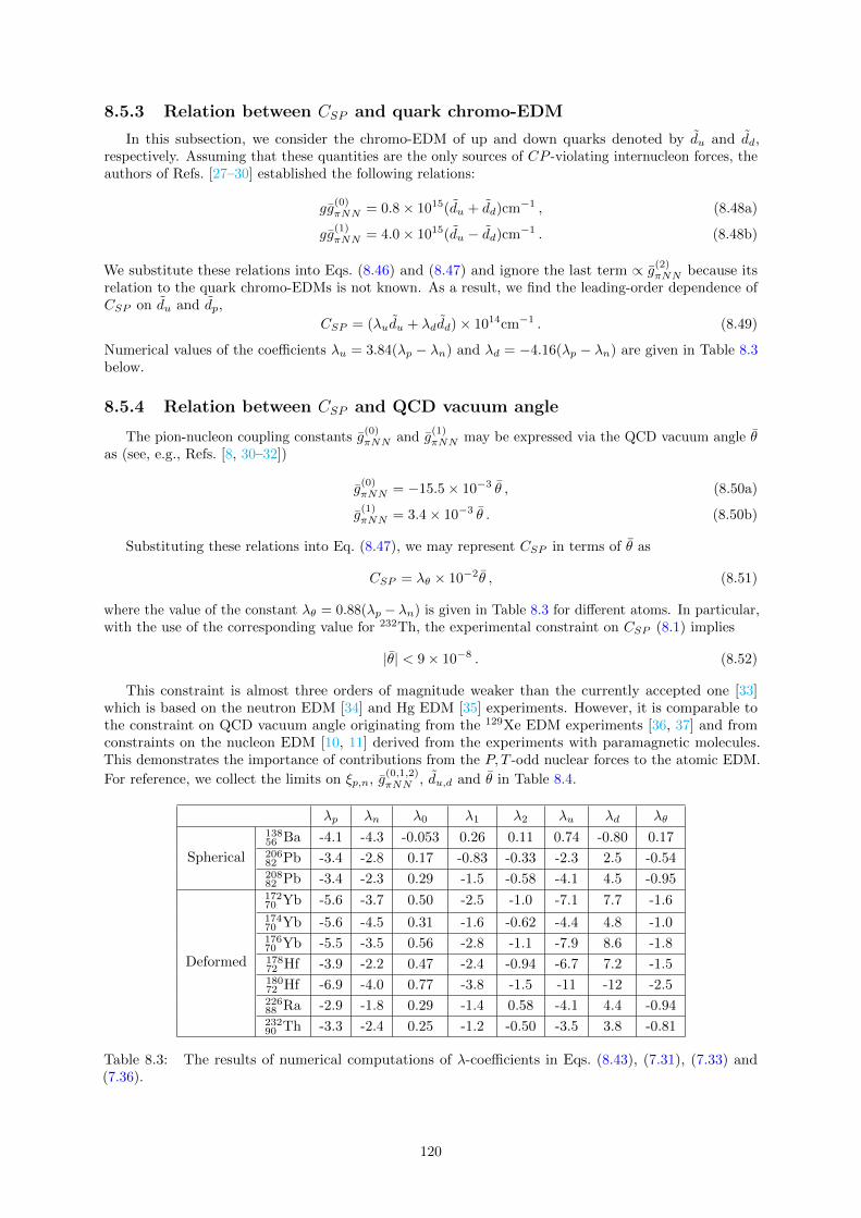
8.5.3 Relation between CSP and quark chromo-EDM

In this subsection, we consider the chromo-EDM of up and down quarks denoted by du and dd,respectively. Assuming that these quantities are the only sources of CP -violating internucleon forces, theauthors of Refs. [27–30] established the following relations:

gg(0)πNN = 0.8× 1015(du + dd)cm−1 , (8.48a)

gg(1)πNN = 4.0× 1015(du − dd)cm−1 . (8.48b)

We substitute these relations into Eqs. (8.46) and (8.47) and ignore the last term ∝ g(2)πNN because its

relation to the quark chromo-EDMs is not known. As a result, we find the leading-order dependence ofCSP on du and dp,

CSP = (λudu + λddd)× 1014cm−1 . (8.49)

Numerical values of the coefficients λu = 3.84(λp − λn) and λd = −4.16(λp − λn) are given in Table 8.3below.

8.5.4 Relation between CSP and QCD vacuum angle

The pion-nucleon coupling constants g(0)πNN and g

(1)πNN may be expressed via the QCD vacuum angle θ

as (see, e.g., Refs. [8, 30–32])

g(0)πNN = −15.5× 10−3 θ , (8.50a)

g(1)πNN = 3.4× 10−3 θ . (8.50b)

Substituting these relations into Eq. (8.47), we may represent CSP in terms of θ as

CSP = λθ × 10−2θ , (8.51)

where the value of the constant λθ = 0.88(λp − λn) is given in Table 8.3 for different atoms. In particular,with the use of the corresponding value for 232Th, the experimental constraint on CSP (8.1) implies

|θ| < 9× 10−8 . (8.52)

This constraint is almost three orders of magnitude weaker than the currently accepted one [33]which is based on the neutron EDM [34] and Hg EDM [35] experiments. However, it is comparable tothe constraint on QCD vacuum angle originating from the 129Xe EDM experiments [36, 37] and fromconstraints on the nucleon EDM [10, 11] derived from the experiments with paramagnetic molecules.This demonstrates the importance of contributions from the P, T -odd nuclear forces to the atomic EDM.

For reference, we collect the limits on ξp,n, g(0,1,2)πNN , du,d and θ in Table 8.4.

λp λn λ0 λ1 λ2 λu λd λθ

Spherical

13856 Ba -4.1 -4.3 -0.053 0.26 0.11 0.74 -0.80 0.1720682 Pb -3.4 -2.8 0.17 -0.83 -0.33 -2.3 2.5 -0.5420882 Pb -3.4 -2.3 0.29 -1.5 -0.58 -4.1 4.5 -0.95

Deformed

17270 Yb -5.6 -3.7 0.50 -2.5 -1.0 -7.1 7.7 -1.617470 Yb -5.6 -4.5 0.31 -1.6 -0.62 -4.4 4.8 -1.017670 Yb -5.5 -3.5 0.56 -2.8 -1.1 -7.9 8.6 -1.817872 Hf -3.9 -2.2 0.47 -2.4 -0.94 -6.7 7.2 -1.518072 Hf -6.9 -4.0 0.77 -3.8 -1.5 -11 -12 -2.522688 Ra -2.9 -1.8 0.29 -1.4 0.58 -4.1 4.4 -0.9423290 Th -3.3 -2.4 0.25 -1.2 -0.50 -3.5 3.8 -0.81

Table 8.3: The results of numerical computations of λ-coefficients in Eqs. (8.43), (7.31), (7.33) and(7.36).

120

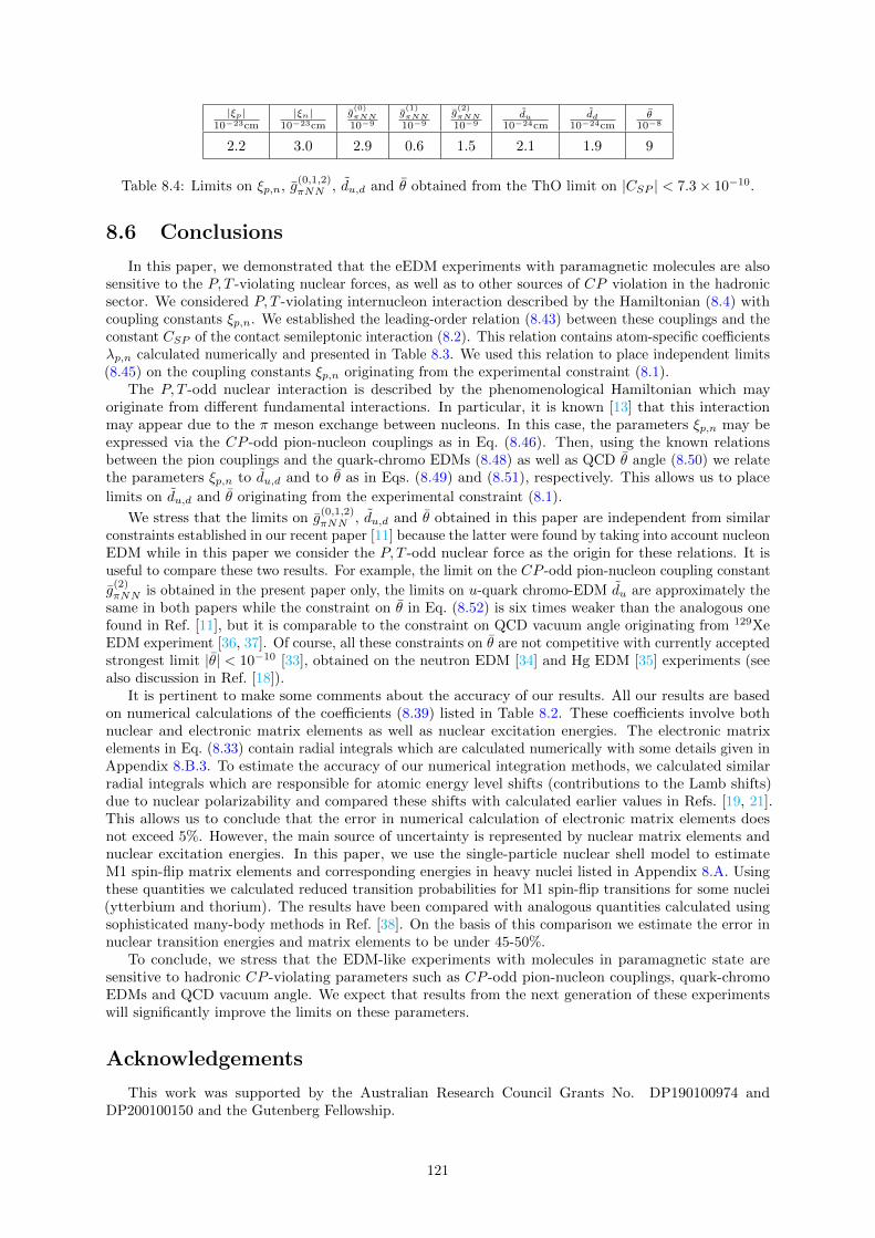
|ξp|10−23cm

|ξn|10−23cm

g(0)πNN

10−9

g(1)πNN

10−9

g(2)πNN

10−9du

10−24cmdd

10−24cmθ

10−8

2.2 3.0 2.9 0.6 1.5 2.1 1.9 9

Table 8.4: Limits on ξp,n, g(0,1,2)πNN , du,d and θ obtained from the ThO limit on |CSP | < 7.3× 10−10.

8.6 Conclusions

In this paper, we demonstrated that the eEDM experiments with paramagnetic molecules are alsosensitive to the P, T -violating nuclear forces, as well as to other sources of CP violation in the hadronicsector. We considered P, T -violating internucleon interaction described by the Hamiltonian (8.4) withcoupling constants ξp,n. We established the leading-order relation (8.43) between these couplings and theconstant CSP of the contact semileptonic interaction (8.2). This relation contains atom-specific coefficientsλp,n calculated numerically and presented in Table 8.3. We used this relation to place independent limits(8.45) on the coupling constants ξp,n originating from the experimental constraint (8.1).

The P, T -odd nuclear interaction is described by the phenomenological Hamiltonian which mayoriginate from different fundamental interactions. In particular, it is known [13] that this interactionmay appear due to the π meson exchange between nucleons. In this case, the parameters ξp,n may beexpressed via the CP -odd pion-nucleon couplings as in Eq. (8.46). Then, using the known relationsbetween the pion couplings and the quark-chromo EDMs (8.48) as well as QCD θ angle (8.50) we relatethe parameters ξp,n to du,d and to θ as in Eqs. (8.49) and (8.51), respectively. This allows us to place

limits on du,d and θ originating from the experimental constraint (8.1).

We stress that the limits on g(0,1,2)πNN , du,d and θ obtained in this paper are independent from similar

constraints established in our recent paper [11] because the latter were found by taking into account nucleonEDM while in this paper we consider the P, T -odd nuclear force as the origin for these relations. It isuseful to compare these two results. For example, the limit on the CP -odd pion-nucleon coupling constant

g(2)πNN is obtained in the present paper only, the limits on u-quark chromo-EDM du are approximately the

same in both papers while the constraint on θ in Eq. (8.52) is six times weaker than the analogous onefound in Ref. [11], but it is comparable to the constraint on QCD vacuum angle originating from 129XeEDM experiment [36, 37]. Of course, all these constraints on θ are not competitive with currently acceptedstrongest limit |θ| < 10−10 [33], obtained on the neutron EDM [34] and Hg EDM [35] experiments (seealso discussion in Ref. [18]).

It is pertinent to make some comments about the accuracy of our results. All our results are basedon numerical calculations of the coefficients (8.39) listed in Table 8.2. These coefficients involve bothnuclear and electronic matrix elements as well as nuclear excitation energies. The electronic matrixelements in Eq. (8.33) contain radial integrals which are calculated numerically with some details given inAppendix 8.B.3. To estimate the accuracy of our numerical integration methods, we calculated similarradial integrals which are responsible for atomic energy level shifts (contributions to the Lamb shifts)due to nuclear polarizability and compared these shifts with calculated earlier values in Refs. [19, 21].This allows us to conclude that the error in numerical calculation of electronic matrix elements doesnot exceed 5%. However, the main source of uncertainty is represented by nuclear matrix elements andnuclear excitation energies. In this paper, we use the single-particle nuclear shell model to estimateM1 spin-flip matrix elements and corresponding energies in heavy nuclei listed in Appendix 8.A. Usingthese quantities we calculated reduced transition probabilities for M1 spin-flip transitions for some nuclei(ytterbium and thorium). The results have been compared with analogous quantities calculated usingsophisticated many-body methods in Ref. [38]. On the basis of this comparison we estimate the error innuclear transition energies and matrix elements to be under 45-50%.

To conclude, we stress that the EDM-like experiments with molecules in paramagnetic state aresensitive to hadronic CP -violating parameters such as CP -odd pion-nucleon couplings, quark-chromoEDMs and QCD vacuum angle. We expect that results from the next generation of these experimentswill significantly improve the limits on these parameters.

Acknowledgements

This work was supported by the Australian Research Council Grants No. DP190100974 andDP200100150 and the Gutenberg Fellowship.

121

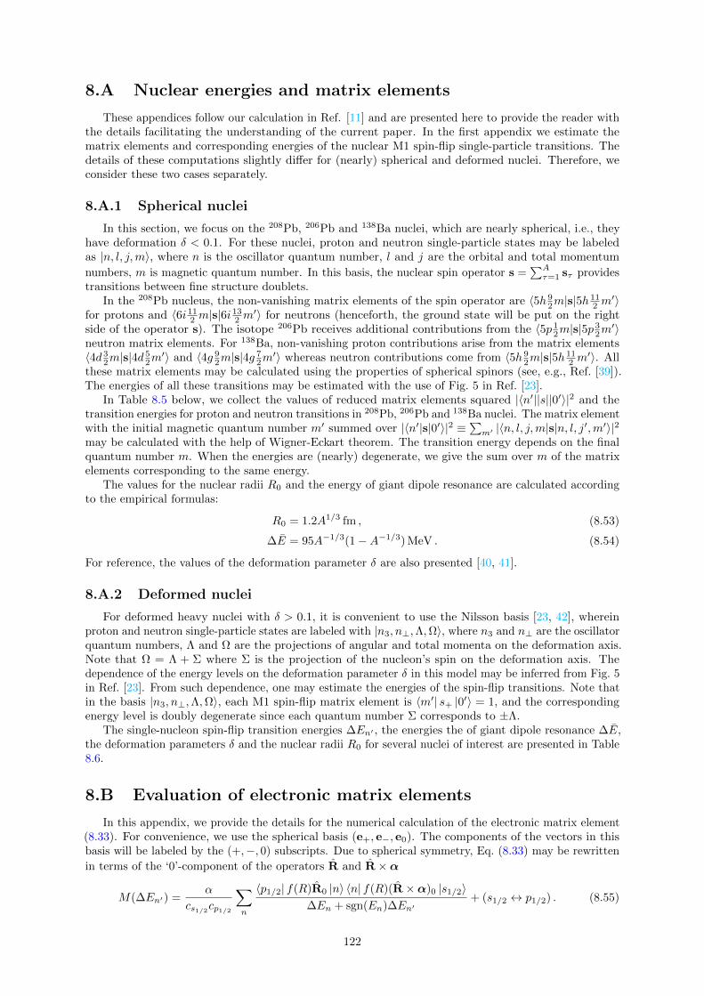
8.A Nuclear energies and matrix elements

These appendices follow our calculation in Ref. [11] and are presented here to provide the reader withthe details facilitating the understanding of the current paper. In the first appendix we estimate thematrix elements and corresponding energies of the nuclear M1 spin-flip single-particle transitions. Thedetails of these computations slightly differ for (nearly) spherical and deformed nuclei. Therefore, weconsider these two cases separately.

8.A.1 Spherical nuclei

In this section, we focus on the 208Pb, 206Pb and 138Ba nuclei, which are nearly spherical, i.e., theyhave deformation δ < 0.1. For these nuclei, proton and neutron single-particle states may be labeledas |n, l, j,m〉, where n is the oscillator quantum number, l and j are the orbital and total momentum

numbers, m is magnetic quantum number. In this basis, the nuclear spin operator s =∑Aτ=1 sτ provides

transitions between fine structure doublets.In the 208Pb nucleus, the non-vanishing matrix elements of the spin operator are 〈5h 9

2m|s|5h112 m

′〉for protons and 〈6i 11

2 m|s|6i132 m

′〉 for neutrons (henceforth, the ground state will be put on the rightside of the operator s). The isotope 206Pb receives additional contributions from the 〈5p 1

2m|s|5p32m′〉

neutron matrix elements. For 138Ba, non-vanishing proton contributions arise from the matrix elements〈4d 3

2m|s|4d52m′〉 and 〈4g 9

2m|s|4g72m′〉 whereas neutron contributions come from 〈5h 9

2m|s|5h112 m

′〉. Allthese matrix elements may be calculated using the properties of spherical spinors (see, e.g., Ref. [39]).The energies of all these transitions may be estimated with the use of Fig. 5 in Ref. [23].

In Table 8.5 below, we collect the values of reduced matrix elements squared |〈n′||s||0′〉|2 and thetransition energies for proton and neutron transitions in 208Pb, 206Pb and 138Ba nuclei. The matrix elementwith the initial magnetic quantum number m′ summed over |〈n′|s|0′〉|2 ≡

∑m′ |〈n, l, j,m|s|n, l, j′,m′〉|2

may be calculated with the help of Wigner-Eckart theorem. The transition energy depends on the finalquantum number m. When the energies are (nearly) degenerate, we give the sum over m of the matrixelements corresponding to the same energy.

The values for the nuclear radii R0 and the energy of giant dipole resonance are calculated accordingto the empirical formulas:

R0 = 1.2A1/3 fm , (8.53)

∆E = 95A−1/3(1−A−1/3) MeV . (8.54)

For reference, the values of the deformation parameter δ are also presented [40, 41].

8.A.2 Deformed nuclei

For deformed heavy nuclei with δ > 0.1, it is convenient to use the Nilsson basis [23, 42], whereinproton and neutron single-particle states are labeled with |n3, n⊥,Λ,Ω〉, where n3 and n⊥ are the oscillatorquantum numbers, Λ and Ω are the projections of angular and total momenta on the deformation axis.Note that Ω = Λ + Σ where Σ is the projection of the nucleon’s spin on the deformation axis. Thedependence of the energy levels on the deformation parameter δ in this model may be inferred from Fig. 5in Ref. [23]. From such dependence, one may estimate the energies of the spin-flip transitions. Note thatin the basis |n3, n⊥,Λ,Ω〉, each M1 spin-flip matrix element is 〈m′| s+ |0′〉 = 1, and the correspondingenergy level is doubly degenerate since each quantum number Σ corresponds to ±Λ.

The single-nucleon spin-flip transition energies ∆En′ , the energies the of giant dipole resonance ∆E,the deformation parameters δ and the nuclear radii R0 for several nuclei of interest are presented in Table8.6.

8.B Evaluation of electronic matrix elements

In this appendix, we provide the details for the numerical calculation of the electronic matrix element(8.33). For convenience, we use the spherical basis (e+, e−, e0). The components of the vectors in thisbasis will be labeled by the (+,−, 0) subscripts. Due to spherical symmetry, Eq. (8.33) may be rewritten

in terms of the ‘0’-component of the operators R and R×α

M(∆En′) =α

cs1/2cp1/2

∑n

〈p1/2| f(R)R0 |n〉 〈n| f(R)(R×α)0 |s1/2〉∆En + sgn(En)∆En′

+ (s1/2 ↔ p1/2) . (8.55)

122

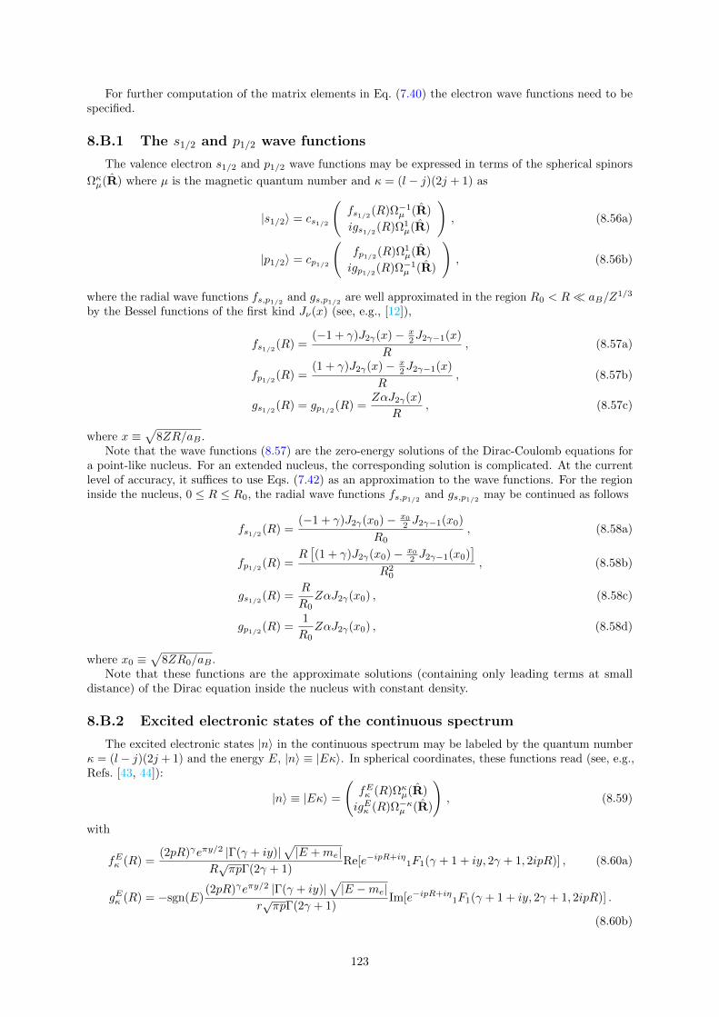
For further computation of the matrix elements in Eq. (7.40) the electron wave functions need to bespecified.

8.B.1 The s1/2 and p1/2 wave functions

The valence electron s1/2 and p1/2 wave functions may be expressed in terms of the spherical spinors

Ωκµ(R) where µ is the magnetic quantum number and κ = (l − j)(2j + 1) as

|s1/2〉 = cs1/2

(fs1/2(R)Ω−1

µ (R)

igs1/2(R)Ω1µ(R)

), (8.56a)

|p1/2〉 = cp1/2

(fp1/2(R)Ω1

µ(R)

igp1/2(R)Ω−1µ (R)

), (8.56b)

where the radial wave functions fs,p1/2 and gs,p1/2 are well approximated in the region R0 < R aB/Z1/3

by the Bessel functions of the first kind Jν(x) (see, e.g., [12]),

fs1/2(R) =(−1 + γ)J2γ(x)− x

2J2γ−1(x)

R, (8.57a)

fp1/2(R) =(1 + γ)J2γ(x)− x

2J2γ−1(x)

R, (8.57b)

gs1/2(R) = gp1/2(R) =ZαJ2γ(x)

R, (8.57c)

where x ≡√

8ZR/aB .Note that the wave functions (8.57) are the zero-energy solutions of the Dirac-Coulomb equations for

a point-like nucleus. For an extended nucleus, the corresponding solution is complicated. At the currentlevel of accuracy, it suffices to use Eqs. (7.42) as an approximation to the wave functions. For the regioninside the nucleus, 0 ≤ R ≤ R0, the radial wave functions fs,p1/2 and gs,p1/2 may be continued as follows

fs1/2(R) =(−1 + γ)J2γ(x0)− x0

2 J2γ−1(x0)

R0, (8.58a)

fp1/2(R) =R[(1 + γ)J2γ(x0)− x0

2 J2γ−1(x0)]

R20

, (8.58b)

gs1/2(R) =R

R0ZαJ2γ(x0) , (8.58c)

gp1/2(R) =1

R0ZαJ2γ(x0) , (8.58d)

where x0 ≡√

8ZR0/aB .Note that these functions are the approximate solutions (containing only leading terms at small

distance) of the Dirac equation inside the nucleus with constant density.

8.B.2 Excited electronic states of the continuous spectrum

The excited electronic states |n〉 in the continuous spectrum may be labeled by the quantum numberκ = (l− j)(2j + 1) and the energy E, |n〉 ≡ |Eκ〉. In spherical coordinates, these functions read (see, e.g.,Refs. [43, 44]):

|n〉 ≡ |Eκ〉 =

(fEκ (R)Ωκµ(R)

igEκ (R)Ω−κµ (R)

), (8.59)

with

fEκ (R) =(2pR)γeπy/2 |Γ(γ + iy)|

√|E +me|

R√πpΓ(2γ + 1)

Re[e−ipR+iη1F1(γ + 1 + iy, 2γ + 1, 2ipR)] , (8.60a)

gEκ (R) = −sgn(E)(2pR)γeπy/2 |Γ(γ + iy)|

√|E −me|

r√πpΓ(2γ + 1)

Im[e−ipR+iη1F1(γ + 1 + iy, 2γ + 1, 2ipR)] .

(8.60b)

123

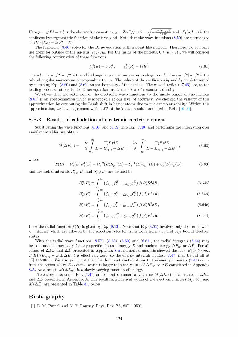
Here p =√E2 −m2

e is the electron’s momentum, y = ZαE/p, eiη =√−κ−iyme/Eγ+iy and 1F1(a, b, z) is the

confluent hypergeometric function of the first kind. Note that the wave functions (8.59) are normalizedas 〈E′κ|Eκ〉 = δ(E′ − E).

The functions (8.60) solve for the Dirac equation with a point-like nucleus. Therefore, we will onlyuse them for outside of the nucleus, R > R0. For the inside of the nucleus, 0 ≤ R ≤ R0, we will considerthe following continuation of these functions

fEκ (R) = b1Rl , gEκ (R) = b2R

l , (8.61)

where l = |κ+ 1/2|−1/2 is the orbital angular momentum corresponding to κ, l = |−κ+ 1/2|−1/2 is theorbital angular momentum corresponding to −κ. The values of the coefficients b1 and b2 are determinedby matching Eqs. (8.60) and (8.61) on the boundary of the nucleus. The wave functions (7.46) are, to theleading order, solutions to the Dirac equation inside a nucleus of a constant density.

We stress that the extension of the electronic wave functions to the inside region of the nucleus(8.61) is an approximation which is acceptable at our level of accuracy. We checked the validity of thisapproximation by computing the Lamb shift in heavy atoms due to nuclear polarizability. Within thisapproximation, we have agreement within 5% of the known results presented in Refs. [19–21].

8.B.3 Results of calculation of electronic matrix element

Substituting the wave functions (8.56) and (8.59) into Eq. (7.40) and performing the integration overangular variables, we obtain

M(∆En′) = −2α

9

∞∫me

T (E)dE

E − Es1/2 + ∆En′− 2α

9

−me∫−∞

T (E)dE

E − Es1/2 −∆En′, (8.62)

whereT (E) = R1

s(E)R1p(E)−R−2

s (E)R−2p (E)− S−1

s (E)S−1p (E) + S2

s (E)S2p(E) , (8.63)

and the radial integrals Rκs,p(E) and Sκs,p(E) are defined by

Rκs (E) ≡∫ ∞

0

(fs1/2f

Eκ + gs1/2g

Eκ

)f(R)R2dR , (8.64a)

Rκp(E) ≡∫ ∞

0

(fp1/2g

Eκ + gp1/2f

Eκ

)f(R)R2dR , (8.64b)

Sκs (E) ≡∫ ∞

0

(fs1/2g

Eκ + gs1/2f

Eκ

)f(R)R2dR , (8.64c)

Sκp (E) ≡∫ ∞

0

(fp1/2f

Eκ + gp1/2g

Eκ

)f(R)R2dR . (8.64d)

Here the radial function f(R) is given by Eq. (8.13). Note that Eq. (8.63) involves only the terms withκ = ±1,±2 which are allowed by the selection rules for transitions from s1/2 and p1/2 bound electronstates.

With the radial wave functions (8.57), (8.58), (8.60) and (8.61), the radial integrals (8.64) maybe computed numerically for any specific electron energy E and nuclear energy ∆En′ or ∆E. For allvalues of ∆En′ and ∆E presented in Appendix 8.A, numerical analysis showed that for |E| > 500me,T (E)/(Es1/2 − E ± ∆En′) is effectively zero, so the energy integrals in Eqs. (7.47) may be cut off at|E| ≈ 500me. We also point out that the dominant contributions to the energy integrals (7.47) comefrom the region where E ∼ 50me, which is larger than the values of ∆En′ or ∆E considered in Appendix8.A. As a result, M(∆En′) is a slowly varying function of energy.

The energy integrals in Eqs. (7.47) are computed numerically, giving M(∆En′) for all values of ∆En′

and ∆E presented in Appendix A. The resulting numerical values of the electronic factors Mp, Mn andM(∆E) are presented in Table 8.1 below.

Bibliography

[1] E. M. Purcell and N. F. Ramsey, Phys. Rev. 78, 807 (1950).

124

[2] T.-D. Lee and C. N. Yang, Tech. Rep., Brookhaven National Lab., Upton, NY (1957).

[3] L. Landau, Sov. Phys. - JETP 5, 336 (1957).

[4] L. Landau, Nuclear Physics 3, 127 (1957).

[5] A. D. Sakharov, Sov. Phys. Usp. 34, 392 (1991).

[6] V. Andreev, D. G. Ang, D. DeMille, J. M. Doyle, G. Gabrielse, J. Haefner, N. R. Hutzler, Z. Lasner,C. Meisenhelder, B. R. O’Leary, et al. (ACME), Nature 562, 355 (2018).

[7] H. Loh, K. C. Cossel, M. C. Grau, K.-K. Ni, E. R. Meyer, J. L. Bohn, J. Ye, and E. A. Cornell,Science 342, 1220 (2013).

[8] N. Yamanaka, B. Sahoo, N. Yoshinaga, T. Sato, K. Asahi, and B. Das, Eur. Phys. J. A 53, 54 (2017).

[9] T. E. Chupp, P. Fierlinger, M. J. Ramsey-Musolf, and J. T. Singh, Rev. Mod. Phys. 91, 015001(2019).

[10] V. V. Flambaum, M. Pospelov, A. Ritz, and Y. V. Stadnik, Phys. Rev. D 102, 035001 (2020).

[11] V. V. Flambaum, I. B. Samsonov, and H. B. Tran Tan, arXiv:2004.10359 (2020).

[12] I. B. Khriplovich, Parity nonconservation in atomic phenomena (Gordon and Breach SciencePublishers, 1991).

[13] O. P. Sushkov, V. V. Flambaum, and I. B. Khriplovich, Zh. Eksp. Teor. Fiz 87, 1521 (1984).

[14] J. Bsaisou, U.-G. Meißner, A. Nogga, and A. Wirzba, Annals Phys. 359, 317 (2015).

[15] M. Denis and T. Fleig, J. Chem. Phys. 145, 214307 (2016).

[16] L. V. Skripnikov, J. Chem. Phys. 145, 214301 (2016).

[17] V. V. Flambaum, I. B. Khriplovich, and O. P. Sushkov, Nucl. Phys. A 449, 750 (1986).

[18] V. V. Flambaum and V. A. Dzuba, Phys. Rev. A 101, 042504 (2020).

[19] G. Plunien, B. Muller, W. Greiner, and G. Soff, Phys. Rev. A 43, 5853 (1991).

[20] K. Pachucki, D. Leibfried, and T. W. Hansch, Phys. Rev. A 48, R1 (1993).

[21] G. Plunien and G. Soff, Phys. Rev. A 51, 1119 (1995).

[22] A. V. Nefiodov, L. N. Labzowsky, G. Plunien, and G. Soff, Phys. Lett. A 222, 227 (1996).

[23] A. Bohr and B. R. Mottelson, Nuclear Structure, vol. 2 (World Scientific, Singapore, 1998).

[24] T. Fleig and M. Jung, J. High Energy Phys. 2018, 12 (2018).

[25] V. V. Flambaum and I. B. Khriplovich, Zh. Eksp. Theor. Fiz 89, 1505 (1985).

[26] W. B. Cairncross, D. N. Gresh, M. Grau, K. C. Cossel, T. S. Roussy, Y. Ni, Y. Zhou, J. Ye, andE. A. Cornell, Phys. Rev. Lett. 119, 153001 (2017).

[27] V. V. Flambaum, D. DeMille, and M. G. Kozlov, Phys. Rev. Lett. 113, 103003 (2014).

[28] M. Pospelov and A. Ritz, Phys. Rev. Lett. 83, 2526 (1999).

[29] M. Pospelov and A. Ritz, Phys. Rev. D 63, 073015 (2001).

[30] M. Pospelov and A. Ritz, Ann. Phys. 318, 119 (2005), special Issue.

[31] J. de Vries, E. Mereghetti, and A. Walker-Loud, Phys. Rev. C 92, 045201 (2015).

[32] J. Bsaisou, C. Hanhart, S. Liebig, U.-G. Meissner, A. Nogga, and A. Wirzba, Eur. Phys. J. A 49, 31(2013).

[33] M. Tanabashi et al. (Particle Data Group), Phys. Rev. D 98, 030001 (2018).

125

[34] C. Abel, S. Afach, N. J. Ayres, C. A. Baker, G. Ban, G. Bison, K. Bodek, V. Bondar, M. Burghoff,E. Chanel, et al., Phys. Rev. Lett. 124, 081803 (2020).

[35] B. Graner, Y. Chen, E. G. Lindahl, and B. R. Heckel, Phys. Rev. Lett. 116, 161601 (2016).

[36] N. Sachdeva, I. Fan, E. Babcock, M. Burghoff, T. E. Chupp, S. Degenkolb, P. Fierlinger, S. Haude,E. Kraegeloh, W. Kilian, et al., Phys. Rev. Lett. 123, 143003 (2019).

[37] F. Allmendinger, I. Engin, W. Heil, S. Karpuk, H.-J. Krause, B. Niederlander, A. Offenhausser,M. Repetto, U. Schmidt, and S. Zimmer, Phys. Rev. A 100, 022505 (2019).

[38] P. Sarriguren, E. Moya de Guerra, and R. Nojarov, Phys. Rev. C 54, 690 (1996).

[39] R. Szmytkowski, J. Math. Chem. 42, 397 (2007).

[40] S. Raman, C. Nestor, and P. Tikkanen, At. Data Nucl. Data Tables 78, 1 (2001).

[41] N. Stone, At. Data Nucl. Data Tables 90, 75 (2005).

[42] S. G. Nilsson, Dan. Mat. Fys. Medd. 29, 1 (1955).

[43] V. B. Berestetskii, E. M. Lifshitz, and L. P. Pitaevskii, Quantum electrodynamics, vol. 4 (Butterworth-Heinemann, 1982).

[44] W. Greiner, Relativistic quantum mechanics: Wave Equations, vol. 2 (Springer, 2000).

126

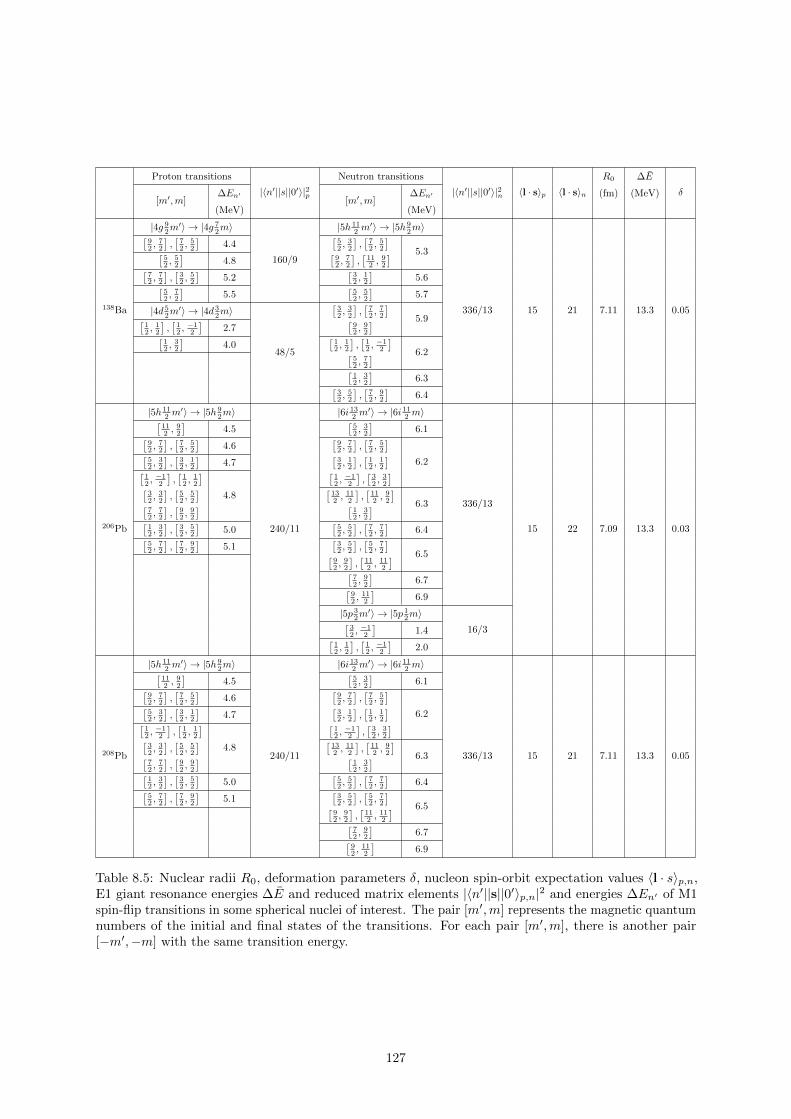
Proton transitions

|〈n′||s||0′〉|2p

Neutron transitions

|〈n′||s||0′〉|2n 〈l · s〉p 〈l · s〉n

R0 ∆E

δ[m′,m]

∆En′[m′,m]

∆En′ (fm) (MeV)

(MeV) (MeV)

138Ba

|4g 92m′〉 → |4g 7

2m〉

160/9

|5h 112 m

′〉 → |5h 92m〉

336/13 15 21 7.11 13.3 0.05

[92 ,

72

],[

72 ,

52

]4.4

[52 ,

32

],[

72 ,

52

]5.3[

52 ,

52

]4.8

[92 ,

72

],[

112 ,

92

][72 ,

72

],[

32 ,

52

]5.2

[32 ,

12

]5.6[

52 ,

72

]5.5

[52 ,

52

]5.7

|4d 52m′〉 → |4d 3

2m〉

48/5

[32 ,

32

],[

72 ,

72

]5.9[

12 ,

12

],[

12 ,−12

]2.7

[92 ,

92

][12 ,

32

]4.0

[12 ,

12

],[

12 ,−12

]6.2[

52 ,

72

][12 ,

32

]6.3[

32 ,

52

],[

72 ,

92

]6.4

206Pb

|5h 112 m

′〉 → |5h 92m〉

240/11

|6i 132 m

′〉 → |6i 112 m〉

336/13

15 22 7.09 13.3 0.03

[112 ,

92

]4.5

[52 ,

32

]6.1[

92 ,

72

],[

72 ,

52

]4.6

[92 ,

72

],[

72 ,

52

]6.2

[52 ,

32

],[

32 ,

12

]4.7

[32 ,

12

],[

12 ,

12

][12 ,−12

],[

12 ,

12

]4.8

[12 ,−12

],[

32 ,

32

][32 ,

32

],[

52 ,

52

] [132 ,

112

],[

112 ,

92

]6.3[

72 ,

72

],[

92 ,

92

] [12 ,

32

][12 ,

32

],[

32 ,

52

]5.0

[52 ,

52

],[

72 ,

72

]6.4[

52 ,

72

],[

72 ,

92

]5.1

[32 ,

52

],[

52 ,

72

]6.5[

92 ,

92

],[

112 ,

112

][72 ,

92

]6.7[

92 ,

112

]6.9

|5p 32m′〉 → |5p 1

2m〉16/3

[32 ,−12

]1.4[

12 ,

12

],[

12 ,−12

]2.0

208Pb

|5h 112 m

′〉 → |5h 92m〉

240/11

|6i 132 m

′〉 → |6i 112 m〉

336/13 15 21 7.11 13.3 0.05

[112 ,

92

]4.5

[52 ,

32

]6.1[

92 ,

72

],[

72 ,

52

]4.6

[92 ,

72

],[

72 ,

52

]6.2

[52 ,

32

],[

32 ,

12

]4.7

[32 ,

12

],[

12 ,

12

][12 ,−12

],[

12 ,

12

]4.8

[12 ,−12

],[

32 ,

32

][32 ,

32

],[

52 ,

52

] [132 ,

112

],[

112 ,

92

]6.3[

72 ,

72

],[

92 ,

92

] [12 ,

32

][12 ,

32

],[

32 ,

52

]5.0

[52 ,

52

],[

72 ,

72

]6.4[

52 ,

72

],[

72 ,

92

]5.1

[32 ,

52

],[

52 ,

72

]6.5[

92 ,

92

],[

112 ,

112

][72 ,

92

]6.7[

92 ,

112

]6.9

Table 8.5: Nuclear radii R0, deformation parameters δ, nucleon spin-orbit expectation values 〈l · s〉p,n,E1 giant resonance energies ∆E and reduced matrix elements |〈n′||s||0′〉p,n|2 and energies ∆En′ of M1spin-flip transitions in some spherical nuclei of interest. The pair [m′,m] represents the magnetic quantumnumbers of the initial and final states of the transitions. For each pair [m′,m], there is another pair[−m′,−m] with the same transition energy.

127

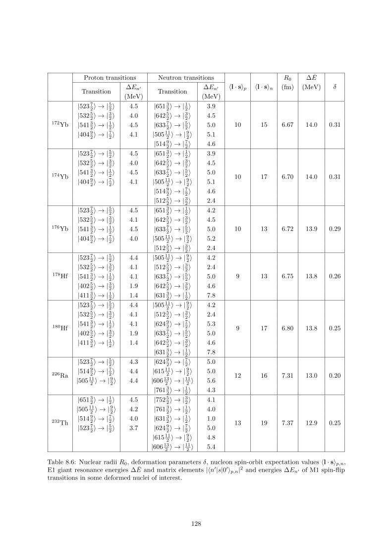
Proton transitions Neutron transitions

〈l · s〉p 〈l · s〉nR0 ∆E

δTransition

∆En′Transition

∆En′ (fm) (MeV)

(MeV) (MeV)

172Yb

|523 72 〉 → |

52 〉 4.5 |651 3

2 〉 → |12 〉 3.9

10 15 6.67 14.0 0.31

|532 52 〉 → |

32 〉 4.0 |642 5

2 〉 → |32 〉 4.5

|541 32 〉 → |

12 〉 4.5 |633 7

2 〉 → |52 〉 5.0

|404 92 〉 → |

72 〉 4.1 |505 11

2 〉 → |92 〉 5.1

|514 92 〉 → |

72 〉 4.6

174Yb

|523 72 〉 → |

52 〉 4.5 |651 3

2 〉 → |12 〉 3.9

10 17 6.70 14.0 0.31

|532 52 〉 → |

32 〉 4.0 |642 5

2 〉 → |32 〉 4.5

|541 32 〉 → |

12 〉 4.5 |633 7

2 〉 → |52 〉 5.0

|404 92 〉 → |

72 〉 4.1 |505 11

2 〉 → |92 〉 5.1

|514 92 〉 → |

72 〉 4.6

|512 52 〉 → |

32 〉 2.4

176Yb

|523 72 〉 → |

52 〉 4.5 |651 3

2 〉 → |12 〉 4.2

10 13 6.72 13.9 0.29

|532 52 〉 → |

32 〉 4.1 |642 5

2 〉 → |32 〉 4.5

|541 32 〉 → |

12 〉 4.5 |633 7

2 〉 → |52 〉 5.0

|404 92 〉 → |

72 〉 4.0 |505 11

2 〉 → |92 〉 5.2

|512 52 〉 → |

32 〉 2.4

178Hf

|523 72 〉 → |

52 〉 4.4 |505 11

2 〉 → |92 〉 4.2

9 13 6.75 13.8 0.26

|532 52 〉 → |

32 〉 4.1 |512 5

2 〉 → |32 〉 2.4

|541 32 〉 → |

12 〉 4.1 |633 7

2 〉 → |52 〉 5.0

|402 52 〉 → |

32 〉 1.9 |642 5

2 〉 → |32 〉 4.6

|411 32 〉 → |

12 〉 1.4 |631 3

2 〉 → |12 〉 7.8

180Hf

|523 72 〉 → |

52 〉 4.4 |505 11

2 〉 → |92 〉 4.2

9 17 6.80 13.8 0.25

|532 52 〉 → |

32 〉 4.1 |512 5

2 〉 → |32 〉 2.4

|541 32 〉 → |

12 〉 4.1 |624 9

2 〉 → |72 〉 5.3

|402 52 〉 → |

32 〉 1.9 |633 7

2 〉 → |52 〉 5.0

|411 32 〉 → |

12 〉 1.4 |642 5

2 〉 → |32 〉 4.6

|631 32 〉 → |

12 〉 7.8

226Ra

|523 72 〉 → |

52 〉 4.3 |624 9

2 〉 → |72 〉 5.0

12 16 7.31 13.0 0.20|514 9

2 〉 → |72 〉 4.4 |615 11

2 〉 → |92 〉 5.0

|505 112 〉 → |

92 〉 4.4 |606 13

2 〉 → |112 〉 5.6

|761 32 〉 → |

12 〉 4.3

232Th

|651 32 〉 → |

12 〉 4.5 |752 5

2 〉 → |32 〉 4.1

13 19 7.37 12.9 0.25

|505 112 〉 → |

92 〉 4.2 |761 3

2 〉 → |12 〉 4.0

|514 92 〉 → |

72 〉 4.0 |631 3

2 〉 → |12 〉 1.0

|523 72 〉 → |

52 〉 3.7 |624 9

2 〉 → |72 〉 5.0

|615 112 〉 → |

92 〉 4.8

|606 132 〉 → |

112 〉 5.4

Table 8.6: Nuclear radii R0, deformation parameters δ, nucleon spin-orbit expectation values 〈l · s〉p,n,E1 giant resonance energies ∆E and matrix elements |〈n′|s|0′〉p,n|2 and energies ∆En′ of M1 spin-fliptransitions in some deformed nuclei of interest.

128

Chapter 9

Time- and parity-violating effects ofnuclear Schiff moment in moleculesand solids

9.1 Overview

As mentioned in Sect. 1.2.2, experiments searching for CP -violation in atoms and molecules oftenattempt to measure the nuclear Schiff moment, which only arises from CP -odd nuclear forces and nucleonEDMs in a finite-sized nucleus. Experimentally, the molecular energy shifts ∆E ∼WSS due to the Schiffmoment S are measured and the value of S may be computed if the quantity WS , which characterizes theinteraction between the Schiff moment and the molecular electrons, is known. In this chapter, I present asimple method through which existing molecular computations of WS may be refined, which will lead tomore precise constraints on the nuclear Schiff moment.

As the result of my research, I have published this paper:

1. V. V. Flambaum, V. A. Dzuba and H. B. Tran TanTime- and parity-violating effects of nuclear Schiff moment in molecules and solidsPhys. Rev. A 101, 042501 (2020), DOI: 10.1103/PhysRevA.101.042501, arXiv:1912.10620.

9.2 Abstract

We show that existing calculations of the interaction between nuclear Schiff moments and electronsin molecules use an inaccurate operator which gives rise to significant errors. By comparing the matrixelements of the accurate and imprecise Schiff moment operators, we calculated the correction factor as afunction of the nuclear charge Z and presented corrected results for the T,P-violating interaction of thenuclear spin with the molecular axis in the TlF, PbO, RaO, TlCN, AcF molecules and in the ferroelectricsolid PbTiO3.

9.3 Introduction

The search for new interactions which violate both the time-reversal (T) and parity (P) invariances isof fundamental importance for the study of Physics beyond the Standard Model. It is well known that,among other phenomena, P,T-odd nuclear interactions give rise to the nuclear Schiff moment [1–4], whichmay interact with electrons and cause measurable shifts in atomic and molecular spectra.

Currently, all calculations of the interaction of nuclear Schiff moments with electrons in moleculesuse an operator which is only approximately correct [2, 5–11]. Although a more accurate form for thisoperator do exist [12], its use has not been widely adopted. In this paper, we demonstrate that theimprecise operator may lead to significant inaccuracy of the results and suggest a simple way to amendthe situation.

The rest of the paper will be organized as follows. In Sect. 9.4, we give a brief review of the variousforms of interaction and the problems associated with them. We will also introduce scaling factors, which

129

are the ratios between the matrix elements of the correct and imprecise operators. These factors maybe used to correct the published results obtained from the imprecise operator. In Sect. 9.5 and 9.6, wepresent the analytical and numerical results for these scaling factors. Sect. 7.7 contains a short summaryof our findings.

9.4 The different forms of interaction

For a pointlike nucleus, the electro-static potential produced by the Schiff moment is presented in theform [1, 3] 1

ϕ0 (R) = 4πS · ∇δ (R) , (9.1)

where R is the electron position vector from the center of the nucleus, δ (R) is the delta function and Sis the nuclear Schiff moment.

Let us consider the matrix element of −eϕ0 between the electronic s and p states, which reads

Msp0 = 4πS ·

(∇ψ†sψp

)R→0

, (9.2)

where ψs,p are the s and p wavefunction for an electron in the potential of a point-like nucleus.We note that although the quantity

(∇ψ†sψp

)R→0

tends toward a constant value for a non-relativisticelectron, it becomes infinite for a relativistic electron. This issue is resolved by considering a finite-sizeinstead of a point-like nucleus. One solution is to simply cut off the point-like-nucleus relativistic electronwavefunction at the surface of the nucleus, obtaining

Msp1 = 4πS ·

(∇ψ†sψp

)R→RN

, (9.3)

where RN is the radius of the nucleus. However, since the variation of ∇ψ†sψp inside the nucleus is of theorder of Z2α2 where Z is the nuclear charge and α is the fine-structure constant, formula (9.3) does notgive reliable results in the case of a heavy nucleus.

Another approach is to use, for the wavefunctions ψs,p, the correct solutions to the Dirac equationwith the potential from a finite-size nucleus. Although in this case, the quantity

(∇ψ†sψp

)R→0

is finite,using Eq. (9.2) to calculate the matrix element is logically inconsistent (since Eq. (9.2) corresponds to theSchiff moment being placed at the center of the nucleus) and may give imprecise results. Unfortunately,this approach in used in all molecular calculations of the effects of nuclear Schiff moments.

A more accurate formula for the potential produced by the nuclear Schiff moment was derived inRef. [12]

ϕ2(R) =3S ·RB

n(R) , (9.4)

where B =∫n (R)R4dR ≈ R5

N and n (R) is nuclear charge density. This formula correspond to aconstant electric field E = −∇ϕ2 produced by the Schiff moment at the center of the nucleus and zerofield outside the nucleus. Here, we see that the actual interaction with the Schiff moment potentialvanishes at the center of the nucleus which explains why placing the Schiff moment at the center of thenucleus as in Eq. (9.2) is not reasonable. However, all molecular calculations used Eq. (9.2).

The corresponding matrix element of −eϕ2 between s and p waves is given by

Msp2 =

3S

B·∫ψ†sRψpn (R) d3R , (9.5)

where ψs,p is the electron wavefunction corresponding to a finite-size nucleus.As we will show below, compared to the correct formula (9.5), Eqs. (9.2) and (9.3) give rise to errors

as large as 20%, which may compromise the reliability of otherwise very accurate atomic and molecularcalculations. In this paper, we present a solution to this problem. We provide the numerical values forthe ratios of the matrix elements

rspcenter =

∣∣∣∣Msp0

Msp2

∣∣∣∣ and rspsurface =

∣∣∣∣Msp1

Msp2

∣∣∣∣ , (9.6)

which can be used to simply rescale any result involving the matrix elements (9.2) and (9.3) to the correctvalue which involves the matrix element (9.5).

1Ref. [1] considered the effects of proton electric dipole moment whereas Ref. [3] consider the effects of P,T-odd nuclearforces which give a bigger contribution to the Schiff moment.

130

9.5 Analytical results

The matrix element (9.2) may be written as [12]

Mspcenter = 3eS · 〈s|n |p〉 Usp (R)

R

∣∣∣∣R→0

, (9.7)

where n = R/R, 〈s|n |p〉 =∫

Ω†snΩp sin θdθdφ and Usp (R) = fs (R) fp (R) + gs (R) gp (R). Here, fs,pand gs,p are the upper and lower component of the electron wave function.

Similarly, the matrix element (9.3) may be written as

Mspsurface = 3eS · 〈s|n |p〉 Usp (R)

R

∣∣∣∣R→RN

, (9.8)

and the matrix element (9.5) as

Mspbody =

15S

R5N

· 〈s|n |p〉∫UspnR

3dR15S

RN· 〈s|n |p〉

∫ 1

0

Usp (x)x3dx , (9.9)

where we have, for simplicity, assumed that the nucleus has a sharp surface, i.e., n (R−RN ) = θ (RN −R)where θ is the Heaviside function. A more accurate numerical calculation will be performed in the nextsection. We found that the difference is insignificant.

Using Eqs. (9.7), (9.3) and (9.5), we may write

rspcenter =Usp (R) /R|R→0

5RN

1∫0

Usp (x)x3dx

, (9.10a)

rspsurface =Usp (R) /R|R→RN5RN

1∫0

Usp (x)x3dx

. (9.10b)

The analytical form of the functions Usp1/2 and Usp3/2 for a finite nucleus may be taken from Ref. [12].

They read2

Usp1/2 (x) ∼ RNx

1− 3

5(Zα)

2x2

[1− 3

14x2 +

2

135x4

]+

81

560(Zα)

4x4

, (9.11a)

Usp3/2 (x) ∼ x

1− 9

20(Zα)

2x2

[1− 69

315x2 +

1

63x4

]+

243

2800(Zα)

4x4

, (9.11b)

which, upon insertion into Eqs. (9.10a) and (9.10b), give

rsp1/2Center ≈

1

1− 0.361(Zα)2

+ 0.08(Zα)4 , (9.12a)

rsp1/2Surface ≈

1− 0.480(Zα)2

+ 0.145(Zα)4

1− 0.361(Zα)2

+ 0.08(Zα)4 , (9.12b)

rsp3/2Center ≈

1

1− 0.270(Zα)2

+ 0.05(Zα)4 , (9.12c)

rsp3/2Surface ≈

1− 0.359(Zα)2

+ 0.09(Zα)4

1− 0.270(Zα)2

+ 0.05(Zα)4 . (9.12d)

The plots of these ratios as functions of the nuclear charge Z are shown in Fig. 9.1.As can be observed from these plots, for small Z, the ratio rspcenter and rspsurface tend to unity which indi-

cates that formulae (9.2) and (9.3) give reasonable estimates of the correct matrix elements. However, forlarge Z, the formula (9.2) presented an overestimate whereas the formula (9.3) presents an underestimateof the result.

2Because we calculate ratios of the matrix elements, the normalization of these functions is not important. Thesefunctions are calculated to the fourth order of Zα, which provides sufficient accuracy, as can be seen from numericalcalculations described in the next section.

131

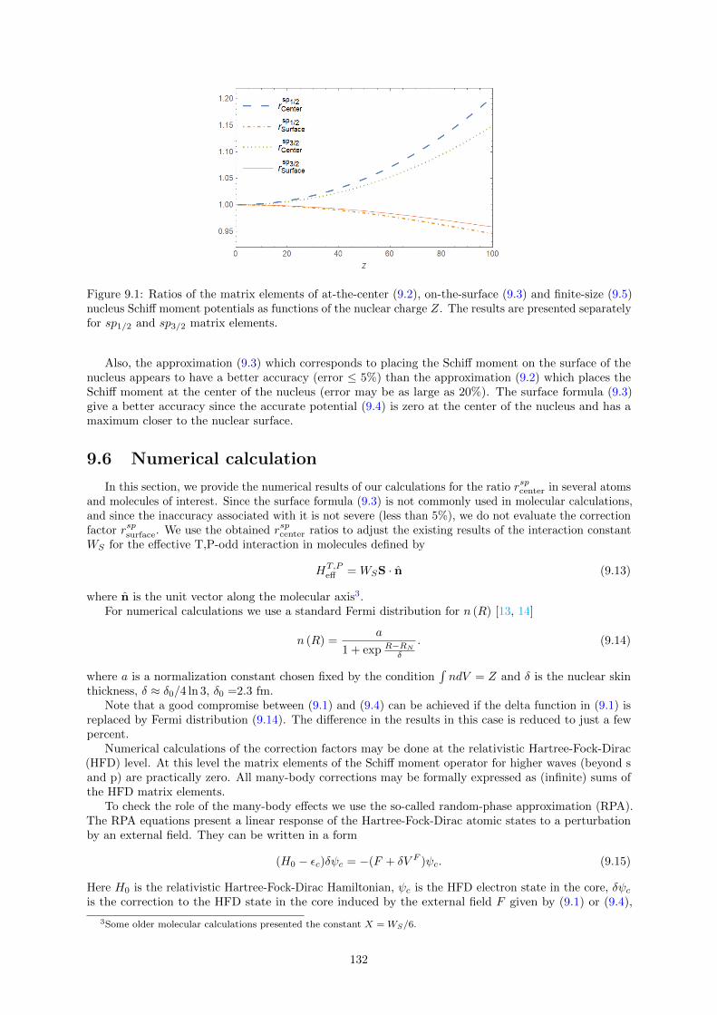
Figure 9.1: Ratios of the matrix elements of at-the-center (9.2), on-the-surface (9.3) and finite-size (9.5)nucleus Schiff moment potentials as functions of the nuclear charge Z. The results are presented separatelyfor sp1/2 and sp3/2 matrix elements.

Also, the approximation (9.3) which corresponds to placing the Schiff moment on the surface of thenucleus appears to have a better accuracy (error ≤ 5%) than the approximation (9.2) which places theSchiff moment at the center of the nucleus (error may be as large as 20%). The surface formula (9.3)give a better accuracy since the accurate potential (9.4) is zero at the center of the nucleus and has amaximum closer to the nuclear surface.

9.6 Numerical calculation

In this section, we provide the numerical results of our calculations for the ratio rspcenter in several atomsand molecules of interest. Since the surface formula (9.3) is not commonly used in molecular calculations,and since the inaccuracy associated with it is not severe (less than 5%), we do not evaluate the correctionfactor rspsurface. We use the obtained rspcenter ratios to adjust the existing results of the interaction constantWS for the effective T,P-odd interaction in molecules defined by

HT,Peff = WSS · n (9.13)

where n is the unit vector along the molecular axis3.For numerical calculations we use a standard Fermi distribution for n (R) [13, 14]

n (R) =a

1 + exp R−RNδ

. (9.14)

where a is a normalization constant chosen fixed by the condition∫ndV = Z and δ is the nuclear skin

thickness, δ ≈ δ0/4 ln 3, δ0 =2.3 fm.Note that a good compromise between (9.1) and (9.4) can be achieved if the delta function in (9.1) is

replaced by Fermi distribution (9.14). The difference in the results in this case is reduced to just a fewpercent.

Numerical calculations of the correction factors may be done at the relativistic Hartree-Fock-Dirac(HFD) level. At this level the matrix elements of the Schiff moment operator for higher waves (beyond sand p) are practically zero. All many-body corrections may be formally expressed as (infinite) sums ofthe HFD matrix elements.

To check the role of the many-body effects we use the so-called random-phase approximation (RPA).The RPA equations present a linear response of the Hartree-Fock-Dirac atomic states to a perturbationby an external field. They can be written in a form

(H0 − εc)δψc = −(F + δV F )ψc. (9.15)

Here H0 is the relativistic Hartree-Fock-Dirac Hamiltonian, ψc is the HFD electron state in the core, δψcis the correction to the HFD state in the core induced by the external field F given by (9.1) or (9.4),

3Some older molecular calculations presented the constant X = WS/6.

132

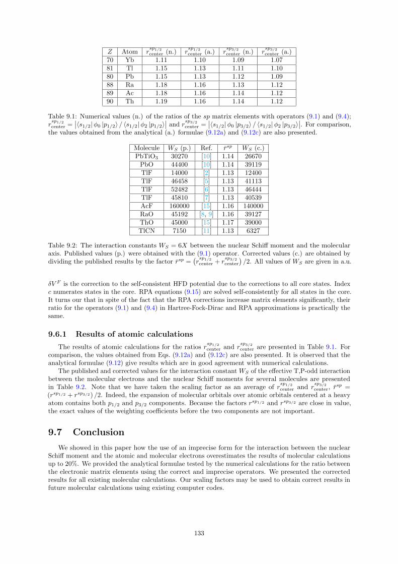
Z Atom rsp1/2center (n.) r

sp1/2center (a.) r

sp3/2center (n.) r

sp3/2center (a.)

70 Yb 1.11 1.10 1.09 1.0781 Tl 1.15 1.13 1.11 1.1080 Pb 1.15 1.13 1.12 1.0988 Ra 1.18 1.16 1.13 1.1289 Ac 1.18 1.16 1.14 1.1290 Th 1.19 1.16 1.14 1.12

Table 9.1: Numerical values (n.) of the ratios of the sp matrix elements with operators (9.1) and (9.4);rsp1/2center =

∣∣〈s1/2|φ0 |p1/2〉 / 〈s1/2|φ2 |p1/2〉∣∣ and r

sp3/2center =

∣∣〈s1/2|φ0 |p3/2〉 / 〈s1/2|φ2 |p3/2〉∣∣. For comparison,

the values obtained from the analytical (a.) formulae (9.12a) and (9.12c) are also presented.

Molecule WS (p.) Ref. rsp WS (c.)PbTiO3 30270 [10] 1.14 26670

PbO 44400 [10] 1.14 39119TlF 14000 [2] 1.13 12400TlF 46458 [5] 1.13 41113TlF 52482 [6] 1.13 46444TlF 45810 [7] 1.13 40539AcF 160000 [15] 1.16 140000RaO 45192 [8, 9] 1.16 39127ThO 45000 [15] 1.17 39000TlCN 7150 [11] 1.13 6327

Table 9.2: The interaction constants WS = 6X between the nuclear Schiff moment and the molecularaxis. Published values (p.) were obtained with the (9.1) operator. Corrected values (c.) are obtained bydividing the published results by the factor rsp =

(rsp1/2center + r

sp3/2center

)/2. All values of WS are given in a.u.

δV F is the correction to the self-consistent HFD potential due to the corrections to all core states. Indexc numerates states in the core. RPA equations (9.15) are solved self-consistently for all states in the core.It turns our that in spite of the fact that the RPA corrections increase matrix elements significantly, theirratio for the operators (9.1) and (9.4) in Hartree-Fock-Dirac and RPA approximations is practically thesame.

9.6.1 Results of atomic calculations

The results of atomic calculations for the ratios rsp1/2center and r

sp3/2center are presented in Table 9.1. For

comparison, the values obtained from Eqs. (9.12a) and (9.12c) are also presented. It is observed that theanalytical formulae (9.12) give results which are in good agreement with numerical calculations.

The published and corrected values for the interaction constant WS of the effective T,P-odd interactionbetween the molecular electrons and the nuclear Schiff moments for several molecules are presentedin Table 9.2. Note that we have taken the scaling factor as an average of r

sp1/2center and r

sp3/2center, r

sp =(rsp1/2 + rsp3/2) /2. Indeed, the expansion of molecular orbitals over atomic orbitals centered at a heavyatom contains both p1/2 and p3/2 components. Because the factors rsp1/2 and rsp3/2 are close in value,the exact values of the weighting coefficients before the two components are not important.

9.7 Conclusion

We showed in this paper how the use of an imprecise form for the interaction between the nuclearSchiff moment and the atomic and molecular electrons overestimates the results of molecular calculationsup to 20%. We provided the analytical formulae tested by the numerical calculations for the ratio betweenthe electronic matrix elements using the correct and imprecise operators. We presented the correctedresults for all existing molecular calculations. Our scaling factors may be used to obtain correct results infuture molecular calculations using existing computer codes.

133

Acknowledgements

This work was supported by the Australian Research Council and the Gutenberg Fellowship.

Bibliography

[1] P. G. H. Sandars, Phys. Rev. Lett. 19, 1396 (1967).

[2] E. A. Hinds and P. G. H. Sandars, Phys. Rev. A 21, 471 (1980).

[3] O. Sushkov, V. Flambaum, and I. Khriplovich, Sov. Phys. - JETP 60, 1521 (1984).

[4] V. Flambaum, I. Khriplovich, and O. Sushkov, Nucl. Phys. A 449, 750 (1986), ISSN 0375-9474.

[5] F. A. Parpia, J. Phys. B 30, 3983 (1997).

[6] H. M. Quiney, J. K. Laerdahl, K. Fægri, and T. Saue, Phys. Rev. A 57, 920 (1998).

[7] A. N. Petrov, N. S. Mosyagin, T. A. Isaev, A. V. Titov, V. F. Ezhov, E. Eliav, and U. Kaldor, Phys.Rev. Lett. 88, 073001 (2002).

[8] V. V. Flambaum, Phys. Rev. A 77, 024501 (2008).

[9] A. D. Kudashov, A. N. Petrov, L. V. Skripnikov, N. S. Mosyagin, A. V. Titov, and V. V. Flambaum,Phys. Rev. A 87, 020102 (2013).

[10] L. V. Skripnikov and A. V. Titov, J. Chem. Phys. 145, 054115 (2016).

[11] A. V. Kudrin, A. Zaitsevskii, T. A. Isaev, D. E. Maison, and L. V. Skripnikov, Atoms 7 (2019).

[12] V. V. Flambaum and J. S. M. Ginges, Phys. Rev. A 65, 032113 (2002).

[13] R. Hofstadter, H. R. Fechter, and J. A. McIntyre, Phys. Rev. 92, 978 (1953).

[14] B. Hahn, D. G. Ravenhall, and R. Hofstadter, Phys. Rev. 101, 1131 (1956).

[15] V. V. Flambaum and V. A. Dzuba, arXiv:1912.03598 (2019).

134

Chapter 10

Conclusions

In this thesis, I explored two new methods for detecting axions in a laboratory, which is important forthe direct detection of Dark Matter.

I demonstrated that by using the axion-photon interference in resonant absorption by atoms andmolecules, one may achieve axion signals that are linear in the axion-normal matter coupling constants.This is in stark contrast with conventional Dark Matter searches whose signals are quadratic or quarticin the underlying coupling constants. As a result, the projected sensitivity of the proposed scheme is atleast an order of magnitude better than those of existing laboratory-based axion experiments.

I also considered a scheme which uses the forward scattering of photons on atoms in media to produceaxions. The axion production rate of this method is proportional to the axion-electron coupling constantsquared, g2

aee, in contrast with conventional photon-axion conversion process, e.g., ALPS and ALPS-II,whose rate is proportional to the axion-photon coupling constant squared, g2

aγγ . This gives a possibilityto measure a different coupling constant.

I also investigated several different methods to circumvent the Schiff’s screening theorem and gaindirect access to the electric dipole moments of nuclei. This is particularly useful since direct measurementsof nuclear electric dipole moments provide information about CP -violation in the hadronic section, theknowledge of which will, in turn, contribute to solving the apparent matter-antimatter asymmetry in theuniverse.

A static external electric field is completely screened by atomic electrons from reaching the atomicnucleus. I studied the mechanism which allows the penetration of an external oscillating electric fieldinside atom or molecule. If the field’s frequency is not in resonance with any atomic or molecular level,the field is only partially screened. On the other hand, if resonance happens then there is a strongenhancement of the field on the nucleus.

I then considered the effects produced by oscillating CP -odd nuclear moments in atoms and molecules.In particular, I showed that an oscillating nuclear electric dipole moment, when coupled with an oscillatingelectric field with the same frequency can give rise to observable nuclear spin precession. I also showedthat oscillating nuclear electric dipole moments, Schiff moments and magnetic quadrupole moments caninduce observable transitions in atoms and molecules. This provides a method for studying axion DarkMatter.

Finally, I studied the effect of the combined electric and magnetic electron-nucleon interaction, whichgives rise to atomic and molecular EDMs. As a result, I was able to place independent constraints onvarious hadronic CP -violating parameters including the nucleon electric dipole moments, the couplingconstants of the CP -odd nuclear forces, the CP -odd pion-nucleon coupling constants, the quark chromo-EDMs as well as the QCD vacuum angle.

135