databases for interval probabilities

Databases for Interval Probabilities

Wenzhong [email protected]

Department of Computer ScienceUniversity of Kentucky

Alex [email protected]


Judy [email protected]


Abstract

In today’s uncertain world, imprecision in probabilistic information is often specified by probabilityintervals. We present here a new database framework for the efficient storage and manipulation ofinterval probability distribution functions and their associated contextual information. While work oninterval probabilities and on probabilistic databases, has appeared before, ours is the first to combinethese into a coherent and mathematically sound framework including both standard relational queriesand queries based on probability theory. In particular, our query algebra allows the user not only to queryexisting interval probability distributions, but also to construct new ones by means of conditionalizationand marginalization, as well as other more common database operations.

1 Introduction

Imagine that there is an election with a surprising outcome: The Rhinoceros Party has won the Senate seatand swept the local elections, contrary to all expectations, and yet the referendum on making AI conferenceslegal has failed, despite the fact that the Rhinoceros Party supports legalization.

What does it mean in such a case that something happens “contrary to all expectations?” Perhaps in thiscase, there were standard indicators that pointed to an Elephant Party win: Elephants raised more moneythan Rhinos and Donkeys combined; Donkeys had more yard signs; pre-election polls showed a clear leadfor the Elephants, and exit polls did as well.

Perhaps an Elephant Party member wishes to file suit against the election commission, based on theseirregularities. In order to do so, they must work with imprecise, probabilistic information, such as “TheMoney-pockets poll indicated an Elephant/Donkey/Rhino split of 62/23/10 for the senate seat, with a marginof error of 2%.”

In order to show bias, the suit must exhibit a breadth of data in a wide variety of formats. Each suchexhibit must be clearly labeled by its origin, format, and any underlying conditionalizing assumptions, suchas “From a poll of Elephant men at their annual county pig roast and fund raiser.”

Whether it is polling data or hospital records, there is always uncertainty in probabilities generated fromdata. And most studies used, whether for risk analysis, medical diagnosis, educational policy, or some othertopic, are based on too-small data sets. There are many ways to indicate uncertainty about probabilities, thesimplest of which is to replace point probabilities with intervals.

Interval probability distributions are robust, and can, in particular, take into account the possibility thatprobability assessments must be combined, although the relationship between them is unknown. For in-

1

stance, two data sets with unknown overlap may have been used to derive these distributions, or the distri-butions may indicate probabilities of events not known to be (or not be) independent.

When interval probability distributions are used for reasoning, whether it is policy development or riskanalysis, they should be stored in a manner easily accessible. It is best for all applications if there is amechanism provided for performing basic probabilistic actions on the data: unions, marginalization, con-ditionalization, and so on. Furthermore, it is extremely useful to be able to access conditionalization infor-mation (“Only Elephants were polled for this,”) or other information that helps put the interval probabilitydistributions into the appropriate context.

We present here a database management framework that does exactly that. While the notion of opera-tions on interval probabilities is not new (see, for instance, [20], etc.), what is new and exciting about thiswork is the framework for automating those operations. Our database management framework allows usersto apply any of the standard operations on interval probabilities, and to reason about the resulting distribu-tions. We automate the notion of a path, by which the genesis of the object is recorded. A path may specifythat this distribution was obtained from data collected and this and the other time, combined using a joinoperation with the specified assumption on the interdependence of the two datasets.

There are several possible interpretations of interval probabilities. We choose the possible world se-mantics [8, 9, 15, 22]. This semantics captures the idea that, while exact probability distributions are notknown, they are known to lie within the given intervals. Using this semantics, we introduce the extendedSemistructured Probabilistic Algebra (ESP-Algebra), an analog of a relational algebra for the SPO datamodel. We define the operations of selection, projection, Cartesian product, join and conditionalization onSPOs and give efficient algorithms to compute them. The SPO data model and the query algebra describedhere provide a flexible solution for representing, storing and querying diverse probabilistic information.

In the next section, we expand on the voting-irregularities example, thus providing instances for many ofthe operations that are formally defined in Section 5. But first we give the basic data model in Section 3, anddiscuss the underlying semantics of interval probability distributions in Section 4. We then put our work intothe context of other work on interval probabilities and probability databases in Section 6. Finally, we putthis work into the bigger picture of Semistructured Probabilistic Databases and their algebras in Section 7.

2 Trouble in Sunny Hill

The town of Sunny Hill is holding elections for the mayor, State Representative and State Senator. Togetherwith these races, residents of Sunny Hill need to vote on two ballot initiatives: whether or not to build anew park downtown and whether or not to legalize AI conferences. Candidates from three parties, Donkey,Elephant and Rhino, are vying for the elected offices and each candidate takes a position on each ballotinitiative, with the Donkey party candidates generally supporting both, Elephant party candidates opposingboth, and Rhino party candidate opposing the park but supporting legal AI.

The public, the candidates and their campaigns, as well as the election commissioner are kept awareof the voting trends in Sunny Hill by polls in the weeks preceding the elections. The polls are conductedamong diverse groups such as representative samples of the entire town population, of likely voters, women,residents of specific neighborhoods, members of specific parties, etc. Among the questions asked on thepolling surveys are current preferences of the participant for each races and about the initiatives, togetherwith some demographic information and some supplementary questions such as whether the participant sawa specific and highly-charged infomercial.

The result of such intensive pre-election polling is that prior to the day of the election, there exists anextensive collection of polling data. Figure 1 contains examples of such data. Before discussing it, let usnotice two important features of pre-election polls.

� Use of intervals. Poll results are constructed by asking a representative sample of a population

2

a sequence of questions and then recording and, later, sorting the answers. However, each samplehas a certain degree of bias, and not every participant reveals his/her true intentions. Because ofthis, pollsters use intervals to represent possible share of voters for each voting pattern. A typicalstatement is “The straight Donkey ticket for the Senate, House and mayoral election is preferred by30% of respondents +/- 2%” (see Poll1 table from Figure 1). We represent such information as theinterval

��.

� Interpretation of statistical distributions. Polling data is typically represented in tables indicatingpercentages of the sample that selected each specific voting pattern. Very often this statistical infor-mation is interpreted probabilistically. For example, the top line of Poll1 table in Figure 1 can beinterpreted as “The probability that a resident of Sunny Hills will vote straight Donkey ticket in theelections is between 28% and 32% based on the October 18 poll.”

Figure 1 shows a small sample of a wide variety of distributions that may be produced by the pollsters.Poll1 is a joint distribution of the expected vote for the three races based on a survey of a representativesample of the entire population of Sunny Hill taken on October 18. Poll2 contains the distribution ofthe vote in the mayoral race and the two ballot initiatives by men affiliated with the Donkey party whointended to vote Donkey in the Senate race, as indicated in a survey conducted on October 26. Poll3 containsinformation about the expected vote on the ballot initiatives by people who intended to split their vote forSenate and mayor between Donkey and Rhino parties respectively. Finally, Poll4, Poll5 and Poll6 containinformation about the expected vote distribution in the mayoral race of the residents of three different partsof Sunny Hill based on the surveys taken on the same day. Sample sizes are also provided for convenience.These and other similar distributions are used by campaign managers and the elections commissioner togain insight into the political trends in Sunny Hill. They are also collected by direct marketing associates.

Given a database of such distributions and the desire for a particular set of probabilities, how can a useraccess that information? Typically, polling data is stored in raw format by polling organizations, often usinga relational DBMS, and is analyzed using a variety of statistical and/or mathematical packages, such as SAS,SPSS or MatLab. This software can be used to construct distributions such as those shown in Figure 1, andperform other manipulations of the data.

Neither traditional relational DBMS nor statistical software deal with storage and retrieval of the proba-bility tables constructed during the analysis. As seen from the examples above, probability distributions arecomplex objects and they are hard to store in traditional relational databases. Yet we want a way to storeprobability tables of varying shapes and sizes, access them readily, and answer a wide variety of queriessuch as:

1. Find all probability distributions for voters from Downtown based on the surveys taken within twoweeks of the election date;

2. Find the distribution of the mayoral vote for likely voters who plan to vote for building a new park;

3. Find all distributions in which the Donkey mayoral candidate receives more than 40% of votes.

To answer these and similar queries, the putative data repository must accept a query language capable ofdealing with probability distributions and all other information associated with them as objects. In additionto that, the query language must be able to manipulate the probability distributions stored in the databaseand perform simple transformations of the distributions according to the laws of probability theory. Forexample, Query 2 (above), applied to a joint distribution of votes for mayoral race and two ballot initiatives(such as Poll2 in Figure 1), should result in the computation of a marginal probability distribution for themayoral vote and the park ballot initiative (by excluding the second initiative from the distribution) andsubsequent conditioning on park=yes.

3

Id: Poll1population: entire towndate: October 18senate house mayor � �Donkey Donkey Donkey 28% 32%Donkey Donkey Elephant 1% 3%Donkey Donkey Rhino 3% 5%Donkey Elephant Donkey 0% 2%Donkey Elephant Elephant 4% 6%Donkey Elephant Rhino 0% 2%Donkey Rhino Donkey 1% 2%Donkey Rhino Elephant 0% 1%Donkey Rhino Rhino 2% 5%Elephant Donkey Donkey 3% 7%Elephant Donkey Elephant 1% 3%Elephant Donkey Rhino 0% 1%Elephant Elephant Donkey 3% 5%Elephant Elephant Elephant 24% 28%Elephant Elephant Rhino 4% 6%Elephant Rhino Donkey 1% 2%Elephant Rhino Elephant 0% 3%Elephant Rhino Rhino 2% 6%Rhino Donkey Donkey 2% 3%Rhino Donkey Elephant 0% 1%Rhino Donkey Rhino 1% 3%Rhino Elephant Donkey 0% 2%Rhino Elephant Elephant 2% 3%Rhino Elephant Rhino 0% 2%Rhino Rhino Elephant 2% 4%Rhino Rhino Elephant 1% 4%Rhino Rhino Rhino 7% 12%

Id: Poll2population: Donkey mendate: October 26senate vote: Donkeymayor park legalization � �Donkey yes yes 44% 52%Donkey yes no 12% 16%Donkey no yes 8% 12%Donkey no no 4% 8%Elephant yes yes 5% 10%Elephant yes no 1% 2%Elephant no yes 3% 4%Elephant no no 6% 8%Rhino yes yes 2% 4%Rhino yes no 1% 3%Rhino no yes 3% 5%Rhino no no 1% 4%

Id: Poll3population: entire towndate: October 22senate vote: Donkeymayor vote: Rhinopark legalization � �yes yes 56% 62%yes no 14% 20%no yes 21% 25%no no 3% 7%

Id: Poll4population: South Sidedate: October 12sample size: 323mayor � �Donkey 20% 26%Elephant 42% 49%Rhino 25% 33%

Id: Poll5population: Downtowndate: October 12sample size: 275mayor � �Donkey 48% 55%Elephant 25% 30%Rhino 20% 24%

Id: Poll6population: West Enddate: October 12sample size: 249mayor � �Donkey 38% 42%Elephant 34% 40%Rhino 15% 20%

Figure 1: Polling Data for Sunny Hills elections.

In this paper, we provide a data model and query language to store, query and manipulate intervalprobability distribution objects. The example indicates the importance of the following features:

� probability distributions and their associated, non-probabilistic information are treated as single ob-jects;

� probability distributions with different structure (e.g., different number/type of random variables in-volved) are stored in the same “relations”;

� query language facilities for retrieval of full distributions based on their properties, and retrieval ofparts of distributions (individual rows of the probability tables) are provided;

4

� query language facilities for manipulations and transformations of probability distributions accordingto the laws of probability theory are provided;

� interval probability distributions are correctly handled.

3 Extended Semistructured Probabilistic Object (ESPO) Data Model

In this section we extend the Semistructured Probabilistic Object (SPO) data model defined in [10] to im-prove the flexibility of the original semistructured data model. We will start by describing the SPO defini-tions from [10], after which the new, extended notion is introduced.

3.1 Simple Semistructured Probabilistic Objects (SPOs)

Consider a universe � of random variables �� . With each random variable �� we associate�� , the set of its possible values. Given a set �� ,�� will denote

�� ! �� "�#� . Let $%� �'& � �� &)( � be a collection of regular relational attributes. For& *$ ,

��'& �will denote the domain of

&. Simple Semistructured Probabilistic Objects (SPOs) are defined as follows.

Definition 1 A Simple Semistructured Probabilistic Object (SPO) + is defined as a tuple +��-,/. � � �10 �3254 ,where(i) .6�7� �'& �18 ��9 & *$ �:8 ��'& � � ( we will refer to . as the context of + );(ii) �;�7�� <� � is a set of random variables that participate in + . We require that �>=�6? ;(iii)

0-@ �� BADC � E ��F �is the probability table of + ;

(iv)2 �;� �HG � �JI � � �� HGLK �JI K � � , where � G � �� GLK � �7M � � and

ION � ��HG N � , F5PRQSPRT , such that�VUWM6�6? . We refer to

2as the set of conditionals of + .

Intuitively, a Simple Semistructured Probabilistic Object (SPO) is defined as a collection of the followingfour different types of information:1. Participating random variables. These variables determine the probability distribution described in anSPO.2. Probability table. This part of the SPO stores the actual numeric probabilities. It is convenient tovisualize the probability table

0as a table of rows of the form

�#XY �[Z � , whereXY �� \� and

Z � 0 ��XY � .Thus, we will speak about rows and columns of the probability table where it makes explanations moreconvenient.3. Conditionals. A probability table may represent a conditional distribution, conditioned by some priorinformation. The conditional part of its SPO stores the prior information in one of two forms: “randomvariable

Ghas value Y ” or “the value of random variable

Gis restricted to a subset

Iof its values”. In our

definition, this is represented as a pair�HG �JI � . When

Iis a singleton set, we get the first type of condition.

4. Context. This part of the SPO contains supporting information for a probability distribution – informationabout the known values of certain parameters, which are not considered to be random variables by theapplication.

3.2 Extended Semistructured Probabilistic Objects (ESPOs)

Extended Semistructured Probabilistic Objects extend the flexibility of SPOs with a number of new features:(i) support for interval probabilities, (ii) association of context and conditionals with individual randomvariables and (iii) paths: information about the origins of the object. We start with formal definitions.

5

Definition 2 Let $ be a context schema. Let � be a set of random variables. An extended context over $and � is a tuple .�� , �'& � �18 � � � � � �� '& ( �18 ( � � ( � 4 � where (i)

& N W$ ,F<PRQ P T

; (ii)8�N ��'& N � ,F�P QSP T

; (iii) � N � � ,F�P Q P T

.

Intuitively, extended context is organized as follows. Given the context . of a Simple SPO and the setof participating random variables � , we associate with each context value the set of random variables forwhich it provides additional information content.

Example 1 Consider the context attributes of the Simple SPO in Figure 2 (left). The Id, population anddate attributes relate to the entire object. At the same time, we would like to represent the fact that 323survey respondents indicated the intention to vote on the park construction question while 342 respondentsresponded to the question about their vote on the AI conference legalization. Without extended context, wecan include both responses:323 and responses:342 in the SPO but we cannot associate the occurrencesof the attributes with individual random variables. The SPO with extended context in the center of theFigure 2 shows how extended context alleviates this problem.

Id: Poll3population: entire townresponses: 323responses: 342date: October 22park legalization �yes yes 0.57yes no 0.2no yes 0.25no no 0.08senate: Donkey

Id: Poll3population: entire townresponses: 323 ��responses: 342 �� date: October 22park legalization �yes yes 0.57yes no 0.2no yes 0.25no no 0.08senate: Donkey

Id: Poll3population: entire townresponses: 323 ��responses: 342 �� date: October 22park legalization �yes yes 0.57yes no 0.2no yes 0.25no no 0.08senate: Donkey ��

Figure 2: Simple vs. Extended context and conditionals in SPOs

We note that in Example 1 the other two context attributes, population and date have the scope overthe entire set of random variables participating in the SPO. This can be represented explicitly, by specifyingthe entire set. However, we will also assume that whenever the scope is not specified for a context attribute,the scope of the attribute is the entire set of participating random variables (as we did here).

Similarly to context, we extend the conditionals.

Definition 3 Let2 � � �HG � �JI � � �� HG ( �JI ( � � be a set of conditionals and � be a set of random vari-

ables s.t., � U � G � �� G ( � �6? . The set of extended conditionals2� is defined as2

� �7� �HG � �JI � � � � � �� HG ( �JI ( � � ( � � � where � N � � ,F5P QSP T

.

Extended conditionals are more subtle than extended context, but they are useful in a number of situa-tions.

Example 2 To continue the previous example, consider now the conditional part of the SPO on the left sideof Figure 2. The condition senate=Donkey applies to the entire distribution. In SPO model only suchconditions can be expressed. As [10, 15] note, this leads to significant restrictions put on query algebraoperations of join and Cartesian product: these two operations are defined only for pairs of SPOs withidentical conditional parts. By extending conditionals to specify scope, as shown in the rightmost SPO onFigure 2, we can extend the expressive power of the framework. The particular SPO in question could have

6

originated as a result of a Cartesian product (See Section 5.4) of an SPO containing information about parkinitiative votes of people who prefer the Donkey party candidate for the Senate and an SPO containing voterpreferences on the AI conference legalization initiative. In the SPO model of [10] this operation would nothave been possible.

We can now give the definition of an Extended SPO (ESPO).

Definition 4 Let C[0,1] be a set of all subintervals of the interval� E ��F �

An Extended Semistructured Prob-abilistic Object (ESPO) + is a tuple +��-,/. �

� � �10 �32 ��S4

, where

� . � is extended context over some schema�

and � ;

� � �7�� <� � is a set of random variables that participate in + . We require that �>=� ? ;�0 @ �� ADC C[0,1] is the probability table of + .

0must be consistent (see Definition 8 in

Section 4);

�2� �7� �HG � �JI � � � � � �� HGD( �JI ( � � ( � � is a set of extended conditionals over � , and

� G � �� GD( � U �;�6? , and

��

, called a path expression or path of + is an expression in the Extended Semistructured ProbabilisticAlgebra.

As mentioned above, in addition to extending context and conditionals and switching to interval prob-abilities, we also introduce a notion of path for an ESPO. Intuitively, the path on an ESPO + indicates itsorigin. If the object was inserted into the database in its current form, then a unique id will be assigned toit. If + appeared as a result of a sequence of query algebra operations, the process of constructing + will bedocumented in its path. The exact syntax and construction of paths will be explained in Section 5.

Example 3 Figure 3 shows the anatomy of ESPOs. The object in the figure represents a joint probabilitydistribution of votes in the Senate race and for the AI conference legalization ballot initiative for male voterswho chose to vote Donkey for mayor. The distribution is based on the survey that took place on October23; 238 respondents indicated their vote in the Senate race, 195 in the legalization vote, with 184 of therespondents giving both answers.

� : Sdate: October 23gender: malerespondents: 238, �� respondents: 195, �� overlap: 184senate legalization [ l, u]Rhino yes [0.04, 0.11]Rhino no [0.1, 0.15]Donkey yes [0.22, 0.27]Donkey no [0.09, 0.16]Elephant yes [0.05, 0.13]Elephant no [0.21, 0.26]mayor: Donkey ��

�� path expression

�� extended context

�� random variables

�� interval probability table

�� extended conditional

Figure 3: Extended Semistructured Probabilistic Object

7

While an ESPO consists of five components, only the first four: extended context, participating randomvariables, probability table and extended conditional carry the information about the distribution. The lastcomponent, the path, allows us to find the origins of a specific ESPO in the database. We note here that anESPO with the same content of the first four components can have different paths in the database (for ex-ample because it could have originated as a results of two syntactically different but semantically equivalentqueries of ESP-Algebra defined below). In many situations it is convenient not to distinguish between suchESPOs. This is formalized in the following definition.

Definition 5 Let +R� ,/. � � � �10 �32 ��S4

and + � � ,/. � � � � � �10 � �32 � � �� 4 be two ESPOs. We say that + isequivalent to + � , denoted +�� + � , iff .�� . � � , �;� � � , 0 � 0 � and

2� � 2 � � .

Note: When representing ESPOs we will assume that a lack of random variables after a context attributeor a conditional indicates that it is associated with all participating random variables. Therefore, strictlyspeaking, we did not need to explicitly include the list of associations for the mayor=Donkey conditionalin Figure 3; we did it to make a point that the conditional part has extended syntax.

4 Semantics for Interval Probabilities

In [10], we assumed for simplicity that all probabilities contained in the SPOs are point probabilities, i.e.theprobability space

� � � E ��F �. This assumption, however, is good only for the situations when we know in

advance that all probabilities computed in a particular application domain will be point probabilities. Thereare many situations that this assumption would not hold.

� In general, when computing the probability of a conjunction of two events, knowing the point prob-abilities of the original events does not immediately guarantee uniqueness of the probability of theconjunction. The latter probability depends also on the known relationship between the two originalevents. When no such relationship is known, the probability of conjunction can only be computed tolie in an interval [4]: �� 8 �� :A F �1E � P � � 8�� P � Q T ��:� 8 � � � � � �J�

� In some applications, it may be infeasible to obtain the exact probabilities or the point probabilitiesobtained will not be robust: so intervals better represent our knowledge of the domain.

In this paper we assume that the probability space is� � C[0,1], the set of all subintervals of the interval� E ��F �

. The rest of this section formally introduces the possible worlds semantics for the probability distribu-tions over

�and the notions of consistency and tightness of the distributions. Possible worlds approach to

describing interval probabilities has been adopted by a number of researchers. In particular, the semanticsdescribed here is similar to the one introduced by de Campos, Huete and Moral [8]. Similar treatment ofinterval probability distributions in database literature appeared in [11] where interval probability distribu-tions were discussed in the context of Temporal Probabilistic Databases. Similar notions are also found inthe work of Weichselberger [22]. In database literature, a specialized version of possible worlds semanticsfor interval probabilities appeared in [11]. The description of the semantics in this section follows [9]. Wediscuss related work in more detail in Section 6.

Definition 6 Let � be a set of random variables. A probabilistic interpretation (p-interpretation) over �is a function �� @ �� C � E ��F �

, such that �� XY � � F.

Given a set of random variables, a p-interpretation over it is any valid point probability distribution.Our main idea is that a probability distribution function (pdf)

0 @ �� C C[0,1] represents a set of

8

possible point probability distributions (a.k.a., p-interpretations). This corresponds to de Campos, et al.’sinstance [8].

In the rest of the paper we will adopt the following notation. Given a probability distribution0 @

�� C C[0,1], for eachXY �� we will write

0 �#XY � � � � �� G �� . Whenever we enumerate��

as�� \� �7� XY � �� XY � , we will write

0 �#XY N � � � � N � G N �,F�P Q P �

.

Definition 7 Let � be a set of random variables and0�@ �� C C[0,1] a complete interval probability

distribution function over � . A probabilistic interpretation � � satisfies0

( ��R9� 0 ) iff��BXY �� J� � � �� P

� � �#XY � P G �� Let � be a set of random variables and

0 � @ I C C[0,1] an incomplete interval probability distributionfunction over

I�� \� . A probabilistic interpretation �� satisfies0 � ( � � 9 � 0 � ) iff

��BXY I � � � �� P� � �#XY � P G ��

Basically, if a p-interpretation �� satisfies an interval probability distribution function0

, then given0

,� � is a possible point probability distribution.

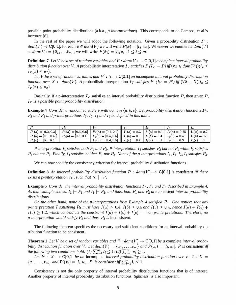
Example 4 Consider a random variable � with domain � 8 � � �� . Let probability distribution functions0 � ,0��

and0�

and p-interpretations � � , � � , � and �� be defined in this table.

� � �� ! "$#%�! &�' ��(�� ! &!#%�! )�' ��(��*�� ! +�#%�$ ,�' ��-�! & ��(��.�-�$ , ��/�$ "�, ��(��*��-�! 0� � ��12��3� �$ &$#%�! +4,�' � � ��12��3� �$ &$#%�! +(' � � ��1�� $ +�#%�! ,�' � � ��12��5�$ & � � ��1��-�! + � � ��1��-�! +�, � � ��1��-�! &� ��62� �� ! &$#7�! ,�' ��(��6��.�3� �$ +!#7�! ,�' ��62��/�$ + ��(��6��.�-�! 98 ��6��-�! & ��(��6��-�

P-interpretation � � satisfies both0 � and

0��. P-interpretation � � satisfies

0��but not

0 � while � satisfies0 � but not0 �

. Finally, � satisfies neither0 � nor

0 �. None of the p-interpretations � � � � � � � � � satisfies

0 .

We can now specify the consistency criterion for interval probability distribution functions.

Definition 8 An interval probability distribution function0 @ �� \� C C[0,1] is consistent iff there

exists a p-interpretation � � , such that ��R9� 0 .

Example 5 Consider the interval probability distribution functions0 � , 0�� and

0�described in Example 4.

As that example shows, � � 9 � 0 � and � � 9 � 0:� , and thus, both0 � and

0��are consistent interval probability

distributions.On the other hand, none of the p-interpretations from Example 4 satisfied

0;. One notices that any

p-interpretation � satisfying0

must have � � 8 �=< E �?>, � � � �=< E �?>

and � � � �@< E �?>, hence � � 8 � � � � �

� � � �@< F"� �, which contradicts the constraint � � 8 � � � � � � � � �� F

on p-interpretations. Therefore, nop-interpretation would satisfy

0Aand thus,

0�is inconsistent.

The following theorem specifies the necessary and sufficient conditions for an interval probability dis-tribution function to be consistent.

Theorem 1 Let � be a set of random variables and0 @ �� SC C[0,1] be a complete interval proba-

bility distribution function over � . Let�� )�%� XY � �� XY � and

0 �#XY N � � � � N � G N �.0

is consistent iffthe following two conditions hold: (1) � NCB � � N P F ; (2) � NCB � G N < F

.Let

0 � @ I C C[0,1] be an incomplete interval probability distribution function over � . LetI �

� XY � �� XY � and0 � �#XY N � � � � N � G N �

.0 � is consistent iff � N�B � � N:P F

.

Consistency is not the only property of interval probability distribution functions that is of interest.Another property of interval probability distribution functions, tightness, is also important.

9

Example 6 Consider the interval probability distribution0

as shown on Figure 4 (left). Assume that0

is complete. It is easy to see that0

is consistent (indeed, the sum of lower bound of probability intervalsadds up to 0.4 and the the sum of the upper bounds adds up to 1.5). In fact, there will be many differentp-interpretations satisfying

0. Of particular interest to us are the p-interpretations that satisfy

0and take

on marginal values. E.g., p-interpretation � � : � � �#XY � �O� E � F�� #XY � �O� E � F�� #XY �O� E � F�� XY ��O� E ��satisfies

0and hits the lower bounds of probability intervals provided by

0for

XY � , XY � andXY . Similarly,

� � : � � �#XY � � � E � �� #XY � � � E � �� #XY � � E � �� #XY �� E � ��satisfies

0and hits the upper bounds of

probability intervals forXY � � XY � and

XY . Thus, every single number in the probability intervals forXY � , XY � andXY is reachable by different p-interpretations satisfying

0.

However, the same is not true forXY . If some p-interpretation � satisfies

0, then � �#XY ��\=� E � F

. Indeed,we know that � �#XY � � � �#XY � � � �#XY �� #XY �B� F

and if � �#XY �B� E � Fthen � �#XY � � � �#XY � � � �#XY �B� E ��

.However, the maximum values for

XY � , XY � andXY allowed by

0are

E � �,E � �

andE �

respectively, and theyadd up to only

E ��.

Similarly, no p-interpretation � satisfying0

can have � �#XY �� E � � . Indeed, in this case, � �#XY � �� #XY � �� XY � � F A E � � � E � �

. However, the smallest values forXY � , XY � and

XY allowed by0

are allE � F

and theadd up to

E � .

� � �� 0.1 0.2� � 0.1 0.2� � 0.1 0.3� � 0.1 0.8

� � �� 0.1 0.2� � 0.1 0.2� � 0.1 0.3� � 0.3 0.7

Figure 4: Tightness of interval probability distributions.

The notion of “reachability” discussed above can be formalized as follows.

Definition 9 Let0 @ I C C[0,1] be an interval probability distribution function over a set of random

variables � . LetI �;� XY � �� XY � and

0 �#XY N �S� � � N � G N �. A number

Z � � N � G N �is reachable by

0atXY N iff

there exists a p-interpretation ��V9� 0 , such that � �#XY N � � Z .

Proposition 1 Let0 @ I C C[0,1] be an interval probability distribution function over a set of random

variables � . If for someXY I there exist

Z, ,

� �� P-Z6P P G �� which are both reachable by0

atXY ,

then any �� Z � � is reachable by0

atXY .

Intuitively points unreachable by an interval probability distribution function represent “dead weight”;they do not provide any additional information about the possible point probability distributions.

Definition 10 Let0-@�I C C[0,1] be an interval probability distribution over a set � of random variables.0

is called tight iff��SXY I � �� Z � � �� G �� Z is reachable by

0atXY .

Example 7 As shown in Example 6, the interval probability distribution function0

shown on the left-handside of Figure 4 is not tight. On the other hand, interval probability distribution function

0 � shown on theright-hand side of Figure 4 is tight. Its tightness follows from the fact that p-interpretations � � and � � fromExample 6 both satisfy it, and now, both upper and lower bounds for

XY are reachable.Function

0 � has another important distinction w.r.t. to0

. Indeed, one can show that for any p-interpretation � , � 9 � 0

iff � 9 � 0 � , i.e., the sets of p-interpretations that satisfy0

and0 � coincide.

Hence, one can say that0 � is a tight equivalent of

0.

10

We will want to replace interval probability distributions that are not tight with their tight equivalents. Thiswill be done using the tightening operator.

Definition 11 Given an interval probability distribution0

, an interval probability distribution0 � is its tight

equivalent iff (i)0 � is tight and (ii) For each p-interpretation � , � 9 � 0 iff � 9 � 0 � .

Proposition 2 Each complete interval probability distribution0

has a unique tight equivalent.

Definition 12 A tightening operator � takes as input an interval probability function0�@�I C C[0,1] and

returns its tight equivalent0 � @ I C C[0,1].

Our next goal is to compute the result of applying the tightening operator to an interval probabilitydistribution function efficiently. First we notice that if

0is tight then � � 0 � � 0 .

The theorem below specifies an efficient procedure for computing the results of tightening an intervalprobability distribution function.

Theorem 2 Let0>@ �� \�!C C[0,1] be a complete interval probability distribution function over a set

of random variables � . Let�� 7� XY � �� XY � and

0 ��XY N � � � � N � G N �. Then

�� F P QBP � �� 0 � �#XY N � � � �� N ��F A

�� B �

G � G N � � �� HG N ��F A�� B �

� � � N � � �

In the rest of the paper we will assume that all ESPOs under consideration have consistent and tightprobability distribution functions. Using the tightening operator according to Theorem 2 will allow us toreplace any probability distribution function that is not tight with its tight equivalent.

Definition 13 An Extended Semistructured Probabilistic Object + � ,/. �� 10 �32 �

��S4is consistent iff

0is consistent. Also, + is tight iff

0is tight.

5 Extended Probabilistic Semistructured Algebra

In the previous two sections we have described the ESPO data model and the underlying semantics for in-terval probability distributions. We are now in position to define the Extended Probabilistic SemistructuredAlgebra (ESP-Algebra). As in [10], we will give definitions for five major operations on the objects: se-lection, projection, Cartesian product, join and conditionalization. In [24] we have described how theseoperations can be defined in a query algebra for interval probability distributions only (without context andconditionals) in a generic way. Here, we ground the operations described in [24] in the ESPO data model.

The first four operations are extensions of the standard relational algebra operations. However, theseoperations will be expanded significantly in comparison both with classical relational algebra [19] and withthe definitions in [10]. The fifth operation, conditionalization, is specific to probabilistic databases andrepresents the procedure of constructing an ESPO containing a conditional probability distribution given anESPO for some joint probability distribution. First proposed as a database operation by Dey and Sarkar [13]for a relational model with point probabilities, this operation had been extended to non-1NF databases in[10].

In the sections below, we will describe each algebra operation. We will base our examples on theelections in Sunny Hill that we have described in Section 2.

Example 8 Figure 5 shows different ESPOs representing a variety of polling data from Figures 1 and 3 andmore. We assume that all these objects have been inserted in the database in their current form, hence, eachreceived a unique path Id.

11

� : � �gender: menparty: Donkeydate: October 26mayor park legaliz- � �

ationDonkey yes yes 0.44 0.52Donkey yes no 0.12 0.16Donkey no yes 0.08 0.12Donkey no no 0.04 0.08Elephant yes yes 0.05 0.1Elephant yes no 0.01 0.02Elephant no yes 0.03 0.04Elephant no no 0.06 0.08Rhino yes yes 0.02 0.04Rhino yes no 0.01 0.03Rhino no yes 0.03 0.05Rhino no no 0.01 0.04senate: Donkey

� : ��date: October 23gender: malerespondents: 238, �� respondents: 195, �� overlap: 184senate legaliz- � �

ationRhino yes 0.04 0.11Rhino no 0.1 0.15Donkey yes 0.22 0.27Donkey no 0.09 0.16Elephant yes 0.05 0.13Elephant no 0.21 0.26mayor: Donkey ��

� � �locality: Sunny Hilldate: October 26park legaliz- � �

ationyes yes 0.56 0.62yes no 0.14 0.2no yes 0.21 0.25no no 0.03 0.07mayor: Donkey

� : � �locality: South Sidedate: October 12sample: 323mayor � �Donkey 0.2 0.26Elephant 0.42 0.49Rhino 0.25 0.33

� : ��locality: Downtowndate: October 12sample: 275mayor � �Donkey 0.48 0.55Elephant 0.25 0.3Rhino 0.2 0.24

� : ��locality: West Enddate: October 12sample: 249mayor � �Donkey 0.38 0.42Elephant 0.34 0.4Rhino 0.15 0.2

� : ��locality: Sunny Hillsdate: October 26sample: 249mayor � �Donkey 0.33 0.39Elephant 0.32 0.37Rhino 0.25 0.3

Figure 5: Sunny Hill pre-election polls in ESPO format.

In a relational data model, a relation is defined as a collection of data tuples over the same set of at-tributes. In our model, an Extended Semistructured Probabilistic relation (ESP-relation) is a set of ESPOsand an Extended Semistructured Probabilistic database (ESP-database) is a set of ESP-relations. Group-ing ESPOs into relations is done not based on structure, as is the case in the relational databases; ESPOswith different structures can co-exist in the same ESP-relation. In the examples below we will considerESP-relation

�;��+ � � + � � + � + � +� � +�� +� � consisting of ESPOs from Figure 5.

5.1 Selection

There is a variety of data stored in a single Extended SPO; for each individual part of the object we needto define a specific version of the selection operation, namely, selection based on context, random variables,conditionals, probabilities and probability table. The first three types of operations, described in Section5.1.1, when applied to an ESP-relation produce a subset of that relation, but individual ESPOs do not change(except for their paths): they either satisfy the query and are returned or do not satisfy it. On the otherhand, selections on probabilities or on probability tables (described in section 5.1.2) may lead to changesin the ESPOs being returned: only parts of the probability tables may “survive” such selection operations.Different types of selections are illustrated in the following example.

Example 9 Table 1 lists some examples of queries that should be expressible as selection queries on ESPOs.For each question we describe the desired output of the selection operation.

Questions 1 – 3 and 5 in the example above do not involve the extensions of the SPO data modelsuggested in Section 3.2. To deal just with these kinds of queries, we could adapt the definitions from ouroriginal SPO algebra of [10]. Questions 4, 6 and 7, however, involve the extensions to the SPO model. Thus,

12

Table 1: Selection queries to ESPOs.

# Query Answer1. “What information is available Set of ESPOs that have date: October 26 in their context.

about voter attitudes on October 26?”2. “What are other voting intentions of Set of ESPOs which have as a conditional mayor=Donkey.

people who choose to vote Donkey for mayor?”3. “What information is known about Set of ESPOs that contain mayor in the set of participating

voter intentions in the mayoral race?” random variables4. “What voting patterns are likely to occur In the probability table of each ESPO, the rows with probability

with probability between 0.2 and 0.3?” values guaranteed to be between 0.2 and 0.3 are found.If such rows exist, they form the probability tableof the ESPO that is returned by the query.

5. “With what probability are voters likely to choose Set of all ESPOs that contain mayor and senate random variables,a Donkey mayor and Elephant Senator? with the probability tables of each containing only the rows

where mayor=Donkey and senate=Elephant.6. “Find all distributions based on more than Set of ESPOs that contain senate random variable and

200 responses about senate vote.” responses = X with�� " �� is associated with it in the context.

7. “How do people who intend to vote Donkey for Set of ESPOs that contain park random variable andmayor plan to vote for the park construction conditional mayor=Donkey is associated with it.ballot initiative?”

the selection definitions from [10] need to be revised to incorporate new types of queries (like 6 and 7) andnew formats for already defined queries (like 4).

5.1.1 Selection on Context, Random Variables and Conditionals

In this section, we define the selection operations that do not alter the content of the selected objects. Westart by defining the acceptable languages for selection conditions for these types of selects.

Recall that the universe $ of context attributes consists of a finite set of attributes& � �� & ( with do-

mains��'& � � �� '& ( � . With each attribute

& *$ we associate a set0�� '& � of allowed predicates.

We assume that equality and inequality are allowed for all& *$ .

Definition 14 1. An atomic context selection condition is an expression�

of the form “&

Q Y (� �'& � Y � )”,

where& *$ , Y ��'& � and

� 0�� '& � .2. An atomic participation selection condition is an expression

�of the form “ � � ”, where � W� is

a random variable.

3. An atomic conditional selection condition is one of the following expressions: “G � � Y � �� Y��

or “G�� Y ” where

G �� is a random variable and Y � Y � �� Y�� HG � . We will slightly abusenotation and write “

G � Y ” instead of “G �;� Y � ”.

4. An extended atomic context selection condition is an expression� � where

�is an atomic context

selection condition and � � � is a set of random variables.

5. An extended atomic conditional selection condition is an expression�� where

�is an atomic con-

ditional selection condition and � � � is a set of random variables.

Example 10 The table below contains some examples of selection conditions of different types for the SunnyHill pre-election polls database.

13

Table 2: Different types of conditions for selection queries.

Selection Condition Type ConditionsContext ��)�� ; �� Extended Context �!�"��$#%��#&��'�� (�)��#��*� � ; +��#��,�� -�.��# ��/�10"�,� � ��32 �Participation �4�10"�� W� ; ��32� W�Conditional �4�10"�� 657�$#�28��0 ; �)��#��&�� :9<;�= #&� ; �)��#%��)�7� 9<;�= #�� 57�$#,2��0 �Extended Conditional �/�10"�,� �65>�$#,28��0 ��32 � ; �)��#��*� �?9@;�= #&� ��%�32 � �4�10"�� ;

Complex selection conditions can be formed as Boolean combinations of atomic selection conditions.The definitions below formalize the selection operation on a single Extended SPO.

Definition 15 Let + � ,/. �� 10 �32 �

��S4be an ESPO and let

� � � �'& � Y � be an atomic context selectioncondition. Let + � � ,/. � � � �10 �32 �

�� 4 where� �:�BA)CED � � ��F . Then CED � + � � ��+:� � iff there exists a tuple�'& �18 � �O�B . � such that

� 8�G � Y � � ; otherwise C D � + � �6? .Definition 16 Let + � ,/. �

� � �10 �32 ��S4

be an ESPO and let�R@ �� be an atomic participation

selection condition. Let + � �-,/. � � � �10 �32 �� 4 where

� ��HA)C D � � ��F . Then C D � + � �7��+:� � iff � � .

Definition 17 Let +-� ,/. �� 10 �32 �


� @ G � � Y � �� Y � � be an atomic con-ditional selection condition. Let + � � ,/. � � � �10 �32 �

�� 4 where� �B�IA)C D � � ��F . Then C D � + �<� ��+:� � iff2

� ��HG �JI � andI �7� Y � �� Y � � .

Let��@ G � Y be an atomic conditional selection condition. Then CJD � + � � ��+:� � iff

2� � �HG �JI � andI � Y .

Definition 18 Let +%� ,/. �� 10 �32 �


� � � �'& � Y � � be an extended atomiccontext selection condition. Let + � �-,/. � � � �10 �32 �

�� 4 where� � �KA)C D � � ��F . Then C D � + � �7��+:� � iff there

exists a tuple�'& �18 � �� . � such that (i)

� 8 G � Y � � ; (ii) � � �ML ; otherwise CED � + � �6? .Definition 19 Let +-� ,/. �

� � �10 �32 ��S4

be an ESPO and let�W@ G � � Y � �� Y � � � be an extended

atomic conditional selection condition. Let + � � ,/. � � � �10 �32 �� 4 where

� � �NA)COD � � ��F . Then CED � + �)��+:� � iff

2� � �HG �JI � �<� � , I �7� Y � �� Y � � , and � � �� .

Let� @ G � Y be an extended atomic conditional selection condition. Then CJD � + �5�>��+ � � iff

2� �

�HG �JI � �<� � , I � Y and � � �� .The semantics of atomic selection conditions discussed so far can be extended to their Boolean combi-

nations in a straightforward manner: CQPQR�PTS � + � �UC P � CEPTS � + �J� and CTPQV,PTS � + � �UC P � + �XWYCEPTS � + � .The interpretation of negation in the context selection condition requires some additional explanation.

In order for a selection condition of the form Z � �'& � Y � to succeed on an ESPO + � ,/. �� 10 �32 �

��S4,

attribute&

must be present in . � . If&

is not present in the context of + , the selection condition does notget evaluated and the result will be ? . Therefore, the statement +R [CJD � + �@W + \CT]�D � + � is not necessarilytrue. This also applies to conditional selection conditions.

Finally, for an ESP-relation

, C P � � ��^ � ��_ � C P � + �J� .We note here that, whenever an ESPO satisfies any of the selection conditions described above, four of

its five components, namely, context, participating variables, probability table and conditional are returnedintact. The only part of the ESPO that changes is its path: the new path expression reflects the fact that theselection query had been applied to the object.

14

Example 11 Consider our ESP-relation

(Figure 5). Below are some possible queries to this relation andtheir results (we specify the unique ids of the ESPOs that match the query).

Id Type Query ResultQ1 context �� !#"$�&%'"$�&( )Q2 participation �+* �,-��.0/ �� ! "$�213"$�&4'"$�&5'"$� ( )Q3 conditionals ��6 ��7��98$:;��7=<-��,�> �� !#"$�&% )Q4 ext. context � � � 6�? 7@��7@� 6�A �@B=B�CD8 6 ��7@��@> �� &E )Q5 ext. context ��F ��7@��G * ��7�CD8 * �-,�@��H ? �@�G<=> �� ! )Q6 ext. conditional � * �,-��G98$:;��7�<��-,=>IC$8 6 ��7��@> �� &E )Q7 ext. conditional � * �,-��G98$:;��7�<��-,=>IC$8 6 ��7��=H J@��K 6 ��> �� L

5.1.2 Selection on Probabilities and Probability Tables

The two types of selections introduced in this section are more complex. The result of a selection operationof either type depends on the content of the probability table, which can be considered as a relation (eachrow being a single record). In the process of performing the probabilistic selection or selection on theprobability table (see questions 4 and 5, Example 9, respectively), each row of the probability table isexamined individually to determine whether it satisfies the selection condition. It is retained in the answerif it does and is thrown out if it does not. Thus, a possible result of either of these two types of selectionoperation is an ESPO with an incomplete probability table. As the selection condition relates only to thecontent of the probability table of an ESPO, its context, participating random variables, and conditionals arepreserved. We start by defining selection on probability tables.

Definition 20 An atomic probabilistic table selection condition is an expression of the form � � Y where�7 ;� and Y �� . Probabilistic table selection conditions are Boolean combinations of atomicprobabilistic table selection conditions.

Definition 21 Let + � ,/. �� 10 �32 �

��S4be an ESPO, � � �� NM � , and let

�<@ � � Y be an atomicprobabilistic table selection condition.

If � W� , then (assuming �O� � N ��F�P QBPPO) the result of selection from + on

�, C D � + � is a semistructured

probabilistic object + � �-,/. � � � �10 � �32 �� 4 , where

� ��HA)COD � � ��F and

QSR �-T0!#"VUWUWUV"=XZY@"VUWUVUI"=T0['�]\_^ Q ��T0! "WUVUWUW"�XZY@"WUVUWUI"�T0[ �ifXZY2\a`�b

undefined ifX�Y]c\a`�U

Example 12 Consider the ESPO + � from Figure 5. The leftmost ESPO of Figure 6 shows the result ofthe selection query on probability table: Ced �gfih B9j �� + � � (find the probability of all voting outcomes whererespondents support the park ballot initiative). Following Definition 21, the result of this query is computedas follows: the context, list of conditionals and participating random variables remain the same, while theprobability table now contains only the rows that satisfy the selection condition and the path changes toreflect the selection operation.

We note that if the same query is applied to the entire relation

, the resulting relation will contain twoESPOs constructed from + � and + : only those ESPOs have participating random variable park (and rowsfor park=yes).

We are now ready to describe the last type of the selection operation: selection on probabilities.

Example 13 The following queries are examples of the types of probabilistic selection queries that need tobe expressible in ESP-Algebra.

1. Find all rows where the lower bound is equal to 0.1;

15

2. Find all rows where the upper bound is greater than 0.4;

3. Find all rows where the probability is guaranteed to be greater than 0.2;

4. Find all rows where the probability can be less than 0.2.

� : �� gender: menparty: Donkeydate: October 26mayor park legaliz- � �

ationDonkey yes yes 0.44 0.52Donkey yes no 0.12 0.16Elephant yes yes 0.05 0.1Elephant yes no 0.01 0.02Rhino yes yes 0.02 0.04Rhino yes no 0.01 0.03senate: Donkey

� : �� date: October 23gender: malerespondents: 238, �� respondents: 195, �� overlap: 184senate legaliz- � �

ationRhino no 0.1 0.15Donkey yes 0.22 0.27Donkey no 0.09 0.16Elephant no 0.21 0.26mayor: Donkey ��

� : �� date: October 23gender: malerespondents: 238, �� respondents: 195, �� overlap: 184senate legaliz- � �

ationRhino yes 0.04 0.11Rhino no 0.1 0.15Donkey no 0.09 0.16Elephant yes 0.05 0.13mayor: Donkey ��

Figure 6: Selection on probability table and probabilities.

The first two queries refer to the lower and upper bounds as supplied by the0

function. The last twoqueries refer to the point probability value as associated with a row by a p-interpretation. The third queryspecifies a for-all condition, which is true iff the condition is true for all p-interpretations satisfying

0.

The fourth query specifies an exists condition, which is true if at least one p-interpretation satisfying0

is satisfies the condition. Our constraint language will allow for all four types of atomic conditions to beexpressed.

Definition 22 An atomic probabilistic selection condition is an expression of one of the forms: (i)� �� Z ;

(ii)G �� Z ; (iii)

� 0 �� Z ; (iv)� 0 �� Z , where

Z � E ��F �and op 7�� =� ��P � < �� . Probabilistic

selection conditions are Boolean combinations of atomic probabilistic selection conditions.

Example 14 While the precise semantics of probabilistic selection conditions is determined in Definition 23below, the following conditions match the probabilistic queries from Example 13: (1)

� � E � F; (2)

G � E �?> ;(3)

� 0 � E � � ; (4)� 0��RE � �

.

Definition 23 Let + � ,/. �� 10 �32 �

��S4be an ESPO. Let

��@ � �� Z � ��@ G �� Z � be a probabilisticatomic selection condition. Let

XY �� \� . The result of selection from + on�

is defined as follows:C�� op � � + � � +:� �-,/. � � � �10 � �32 �

�� 4 , where� � � A)COD � � ��F and

0 � �#XY � � 0 �#XY � if

� �� Z �HG �� Z � �undefined otherwise.

Let� @ � 0 �� Z be a probabilistic atomic selection condition. The result of selection from + on

�is

defined as follows: C!� op � � + � � + � �-,/. � � � �10 � �32 �� 4 , where

� � � A)COD � � ��F and

0 � �#XY � � 0 �#XY � if

�� 9 � 0 � � � ��XY �X�� Z � �undefined otherwise.

Let� @ � 0 �� Z be a probabilistic atomic selection condition. The result of selection from + on

�is

defined as follows: C!� op � � + � � +:� �-,/. � � � �10 � �32 �� 4 , where

� � � A)COD � � ��F and

0 � �#XY � � 0 �#XY � if

�"� � 9 � 0 � � � ��XY �X�� Z � �undefined otherwise.

16

Example 15 The center and the rightmost ESPOs on Figure 6 represent the results of selections on proba-bilities: C �� + � � and C �� J� � + � � respectively. In both cases, the results of the selection keep the samecontext, conditionals and participating random variables, while the probability table is modified to retainonly the rows where the upper (lower) bound on the probability interval satisfies the selection condition.

Notice that the result of C �� would contain seven ESPOs: every object in

contains rows whereupper bound on probability is greater that 0.14. The result of C �� J� � � will contain two ESPOs constructedfrom + � and + � : only those had rows with lower probability less than 0.11.

While evaluation of the probabilistic selection conditions on lower and upper bounds is fairly straight-forward, evaluation of the probabilistic selection conditions referring to p-interpretations may seem to becomplex. As it turns out, these conditions can be expressed via the conditions on upper and lower boundsas specified in the following proposition.

Proposition 3 The following equivalences hold:�-conditions

�-conditions

C � � B � � � � �UC �B � R � B � � � C �� B � � � � � C �� R ��

C � � �� UC �� C �� C �� C � � �� UC �� C �� C �� C � � �� UC �� C �� C �� C � � �� UC �� C �� C �� C � ��

B � � � � �UC �� V �� C �� B � � � � � C � �

B � V � �B � � �Example 16 Figure 7 shows some selections on probabilities that use p-interpretation notation. First query,C � �� J� � + � � finds all rows in the probability table of + � for which all p-interpretations have probabilityless than 0.11. By Proposition 3, this query is equivalent to C �� J� � + � � . Second query, C � � �� + � � asksfor rows of the probability table of + � in which at least one satisfying p-interpretation can have probabilityless than or equal to 0.04. By Proposition 3, it is equivalent to C �� + � � .

� : �� gender: menparty: Donkeydate: October 26mayor park legalization � �Donkey no no 0.04 0.08Elephant yes yes 0.05 0.1Elephant yes no 0.01 0.02Elephant no yes 0.03 0.04Elephant no no 0.06 0.08Rhino yes yes 0.02 0.04Rhino yes no 0.01 0.03Rhino no yes 0.03 0.05Rhino no no 0.01 0.04senate: Donkey

� : �� gender: menparty: Donkeydate: October 26mayor park legalization � �Donkey no no 0.04 0.08Elephant yes no 0.01 0.02Elephant no yes 0.03 0.04Rhino yes yes 0.02 0.04Rhino yes no 0.01 0.03Rhino no yes 0.03 0.05Rhino no no 0.01 0.04senate: Donkey

Figure 7: Probabilistic selection on� 0

and� 0

conditions.

Different selection operations (both described in this section and in Section 5.1.1) commute, as shownin the following theorem:

Theorem 3 Let�

and� � be two selection conditions and let

be a semistructured probabilistic relation.

Then COD � C D S � � �UC D S � COD � �J� �

17

5.2 Projection

Projection in classical relational algebra removes columns from the relation and, if needed, collapses dupli-cate tuples. ESPOs consist of four different components that can be affected by projection operation. Wedistinguish between three different types of projection here: on context, on conditionals and on participatingrandom variables, the latter, affecting probability table as well.

There are two issues that need to be addressed when defining projection on context. First, contexts maycontain numerous copies of relational attributes. Hence, projecting out a particular attribute from a contextof an ESPO should result in all copies if this attribute being projected out. The second issue is the fact thatin extended context, different attributes are associated with different participating random variables. Thus,it would be desirable to be able to take these associations into account when performing projections.

To address these two issues we define two types of projection on context. The first operation will besimilar to standard relational projection, while the second operation will work by removing associationsbetween context attributes and random variables.

Definition 24 Let �7�7� & � �� & M � be a set of context attributes and +��-,/. �� 10 �32 �

��S4be an ESPO.

Projection of + on � , denoted �� + � is an ESPO + ��,/. � S � � �10 �32 �� 4 , where . � S �7� �'& �18 � � L ��9 �'& �18 �

� L �B . � � & �� and� � � A�� F .

Definition 25 Let � � � � �'& � � � � � �� '& M � ��M�� be a set of pairs where forF6P Q P O

,& N

a con-text attribute and � N � � . Let + � ,/. � � � �10 �32 �

��S4be an ESPO. Projection of + on � � , denoted

� �� + � is an ESPO + � � ,/.�� S � � �10 �32 �� 4 , where .�� S � � �'& �18 � � � ��9 �'& �18 � � L�� V. � � & � & N

� & � �� & M � � for someF�P Q PPO �

and ?*=� �5� � � L U � N � and� � � A�� F .

Given an ESPO + and a set of pairs � � as described in Definition 25, the projection operation willproceed as follows. The set of context attributes to keep which comes from � � specifies for each attributethe list of random variables for which it is allowed to be kept. The projection operation (i) removes fromthe input ESPO + all attributes not in � � and (ii) for each instance

� 8 � � L�� . � of attribute& N

s.t.,�'& N � � N � �� it will remove all references in � L that are not in � N . If � L U*� N �6? , then� 8 � � L � is omitted

from the projection. Projections on context are illustrated in the example below.

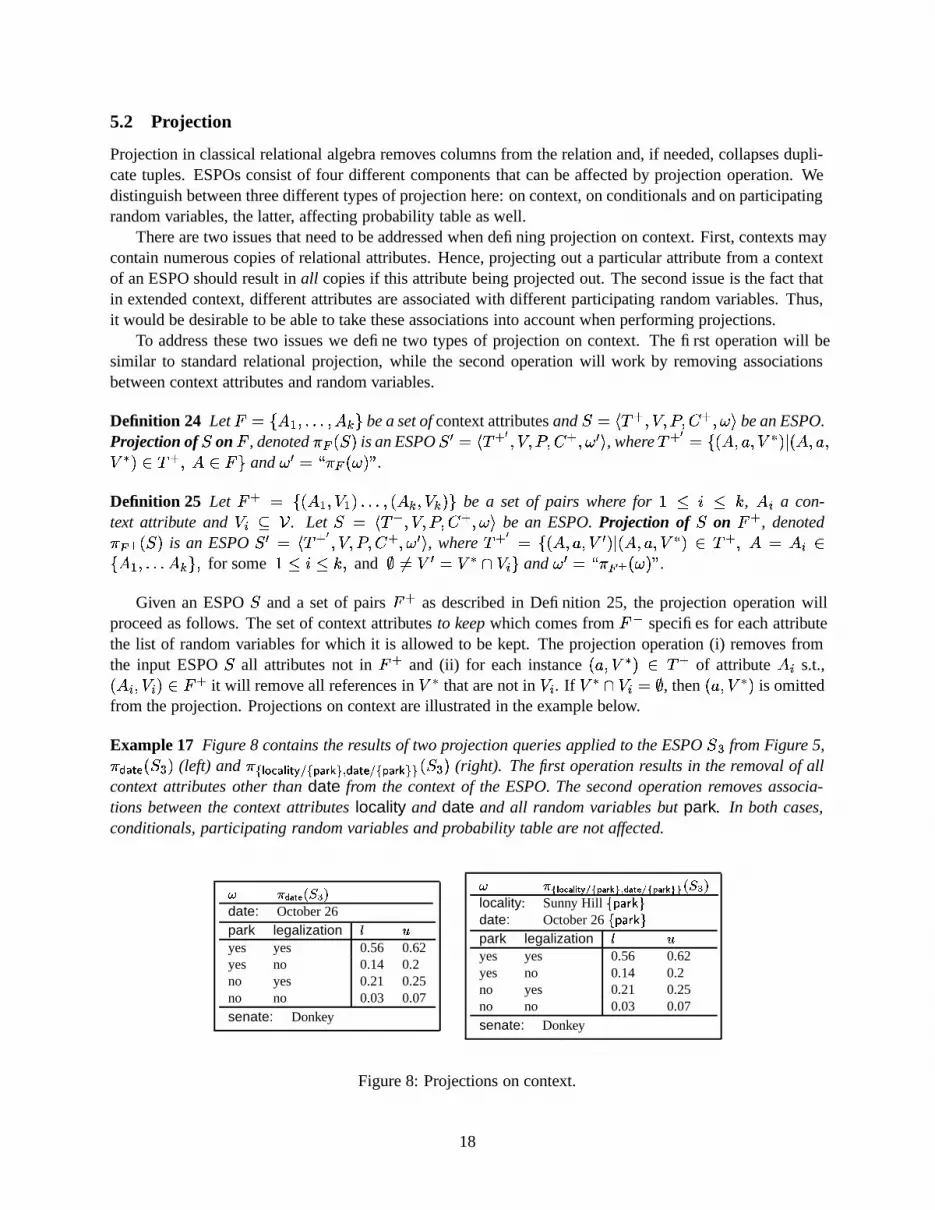
Example 17 Figure 8 contains the results of two projection queries applied to the ESPO + from Figure 5,�� + � (left) and � ��

j�� d �gfih�� d �$f�h�� + � (right). The first operation results in the removal of all

context attributes other than date from the context of the ESPO. The second operation removes associa-tions between the context attributes locality and date and all random variables but park. In both cases,conditionals, participating random variables and probability table are not affected.

�� date: October 26park legalization � �yes yes 0.56 0.62yes no 0.14 0.2no yes 0.21 0.25no no 0.03 0.07senate: Donkey

�� ! � �� "� �� locality: Sunny Hill ��date: October 26 ��park legalization � �yes yes 0.56 0.62yes no 0.14 0.2no yes 0.21 0.25no no 0.03 0.07senate: Donkey

Figure 8: Projections on context.

18

Projection operations on conditionals can be defined similarly. We note here that, while syntacticallythese operations are similar, projecting conditionals out of ESPOs is a more dangerous operation from theprobability theory point of view. Basically, it is taking a conditional probability distribution

0 �� 9 I � andmaking a decision to “forget” the conditioning information

I, and refer to the distribution as

0 �� fromthen on. If unconditional distribution

0 �� is also available, this may lead to some confusion. However,in some cases, projecting out conditionals is meaningful: when a specific random variable is removed fromconsideration in the entire database, it needs to be projected out from both lists of participating randomvariables (see below) as well as from the conditionals of affected ESPOs. Similarly, if the users switch toa sub-database, all ESPOs in which contain the same conditional part, that conditional part can be removedfor convenience. With this in mind we present the projection on conditionals.

Definition 26 Let M � � G � �� G M � � � be a set of random variables and + � ,/. �� 10 �32 �

��S4be

an ESPO. Projection of + on M , denoted � P�� + � 1 is an ESPO + � � ,/. � � � �10 �32 � S �� 4 , where2� S �

� �HG �JI � � L ��9 �HG �JI � � L �B 2 ��

andG M � and

� � � A�� P�� F .Definition 27 Let M � � � �HG � � � � � �� HG M � �ZM�� be a set of pairs where for all

F P Q<P O,G N � and

� N � � . Let +R� ,/.�� 10 �32 �

��S4be an ESPO. Projection of + on M � , denoted � P�� + � is an ESPO

+ � � ,/.�� 10 �32 � S �� 4 , where

2� S � � �HG �JI � � � ��9 �HG �JI � � L#� -. � � G � G N � G � �� G M � , and

?*=� �� L U � N � ; � �� A�� P�� F .The following example illustrates how projection operations on conditionals work.

Example 18 Figure 9 shows the results of two different projection on conditionals operations, �� + � �(left) and ��

j�If � �� + � � (right). The first projection removes all conditionals in + � , leaving the

conditional component empty. The second projection severs the association between the �4�10"�� 657�$#�28��0conditional and the random variable legalization. Context, random variables and probability table are leftintact.

: �� date: October 23gender: malerespondents: 238, �� respondents: 195, �� overlap: 184senate legalization � �Rhino yes 0.04 0.11Rhino no 0.1 0.15Donkey yes 0.22 0.27Donkey no 0.09 0.16Elephant yes 0.05 0.13Elephant no 0.21 0.26

: � �� (�� date: October 23gender: malerespondents: 238, �� respondents: 195, �� overlap: 184senate legalization � �Rhino yes 0.04 0.11Rhino no 0.1 0.15Donkey yes 0.22 0.27Donkey no 0.09 0.16Elephant yes 0.05 0.13Elephant no 0.21 0.26mayor: Donkey ��

Figure 9: Projections on conditionals.

Now we are ready to define the most intricate projection operation, projection on the set of randomvariables. When defining this operation, we need to keep in mind the following: (i) projection is only allowed

1Symbol “C” is used in the notation to distinguish the projection operation from the projection on the set of participating randomvariables, to be defined below.

19

if at least one random variable remains in the resulting set of participating random variables 2; (ii) projectingout a random variable � should result in removal of � from the extended context and conditionals; (iii)projecting out a random variable � should remove this variable from the probability table, i.e. the underlyingprobability distribution function will change. Out of these notes, the last is of the most importance.

Definition 28 Let +V� ,/. �� 10 �32 �

��S4be an ESPO, and let � L � � . Projection of + on � L , denoted

� �� + � is defined as follows:

1. � L U �;�6? : � � � � + � �6? .2. � L U �;� �5�:=� ? : � �� + � � +:� �-,/. � S � �� 10 � �32 � S �� 4 , where

� .�� S �7� �'& �18 �� 9 �'& �18 �� *. � and� U �ML�=�6? and

� � � � U ��L ��2� S �7� �HG �JI �� 9 �HG �JI �� 2 � and

� U �ML�=�6? and� � � � U �ML �

�0 � @ �� C C[0,1].For all

XY � �� and� XY � � XY � � �B �� ,

0 � � XY � � � � �� B � ��

� �� S � �� S S � �� XY � � XY � � �J� � �� B � �

�

� �� S � �� S S � �� XY � � XY � � �J� � �

�� A�� F

This definition requires a careful explanation. Let + ��,/. � � � �10 �32 ��S4

be an ESPO, and let � L � �be the set of projection random variables. The computation of � � � � + � proceeds as follows. First, we checkif the intersection of � , the set of participating random variables of + and � L is empty, and if it is, we returnempty set as the answer. If �<� � � U � L is not empty, we build the projection as follows:

(i) the new set of participating random variables is � � ;(ii) the new context . � S and conditionals

2� S are produced from . � and

2� respectively, by eliminating

all random variables not from �\� from the extensions (associations). Context entries (conditionals)from . � (

2� ) associated only with variables not from �� will be eliminated from . � S (

2� S );

(iii) finally, the new probability table function is defined as follows. The function must range over�� .

As � � � � , with each valueXY � �� , a set of values

� XY � � XY � � � �� is associated, whereXY � � ranges over�� 7A �5� � . Given a p-interpretation � 9 � 0 , for each

XY � �� we can com-pute the probability assigned to it by

0as � � XY � � � � �� S S �� S � � � XY � � XY � � � � Now, we know that the

probability ofXY � has to range between the minimal and maximal value of � � XY � � , for all � 9 � 0

. Thisinterval,

� �� B � � � XY � � � � �� B � � � XY � � � is defined to be the value of the new probability distributionfunction

0 � onXY � .

While the computation of the new set of participating random variables, context and conditionals accord-ing to Definition 28 is straightforward, computing the new probability table requires solving a number ofoptimization problems (finding �� s and � �� s of � � � XY � � XY � � � for all

XY � ), which seems like a fairly tedioustask. However, it turns out that these optimization problems have analytical solutions.

2We want our query algebra to be closed: ESPOs in — ESPOs out. Removing all random variables from the ESPO basicallycollapses it. The object returned by such an operation will no longer satisfy our definition of an ESPO. Because of that, we do notconsider such operations.

20

Theorem 4 Let +��-,/. � � � �10 �32 ��S4

be an ESPO and � L � � . Let � U � L =�6? and +:� �-,/. � S � �� 10 � �2� S �� 4 � � �� + � . Let

0 � � � Y � � � � � � �� S � �� S S � �� S � �� S S � � �� F � � � �� S � �� S S � �� G � �� S � �� S S � � � �Then,

0 � � � � � 0 � � � .The projection on the set of random variables is illustrated in the example below.

Example 19 Figure 10 illustrates the process of computing projection � �� + � � on participating ran-

dom variables. The first step of this operation is the removal of all other random variables from the proba-bility table. Next, the duplicate rows of the new probability table are collapsed and the probability intervalsare added. After that, the operation on tightening is performed to find the true intervals as we can observethat neither of the three lower bounds is reachable. We then exclude respondents:195 from the context asit is not associated with senate variable and disassociate legalization with conditionals.

� : � �date: October 23gender: malerespondents: 238, �� respondents: 195, �� overlap: 184senate legalization � �Rhino yes 0.04 0.11Rhino no 0.1 0.15Donkey yes 0.22 0.27Donkey no 0.09 0.16Elephant yes 0.05 0.13Elephant no 0.21 0.26mayor: Donkey ��

B��

� : � � � �� date: October 23gender: malerespondents: 238, �� respondents: 195, �� overlap: 184senate � �Rhino 0.04 0.11Rhino 0.1 0.15Donkey 0.22 0.27Donkey 0.09 0.16Elephant 0.05 0.13Elephant 0.21 0.26mayor: Donkey ��

B��

� : � � � � �� date: October 23gender: malerespondents: 238, �� overlap: 184senate � �Rhino 0.14 0.26Donkey 0.31 0.43Elephant 0.26 0.39mayor: Donkey ��

B��

� : � � � �� date: October 23gender: malerespondents: 238, �� overlap: 184senate � �Rhino 0.18 0.26Donkey 0.35 0.43Elephant 0.31 0.39mayor: Donkey ��

Figure 10: Projection on the participating random variables.

5.3 Conditionalization

Conditionalization was first considered as an operation of a relational algebra related to a probabilisticdata model by Dey and Sarkar [13]; Classical relational algebra has no prototype of it. Intuitively, condi-tionalization is the operation of computing a conditional probability distribution, given a joint probabilitydistribution. To simplify the definition below, we will employ the following notation. Let � �7�� ( �be a set of random variables and let � � and � � � � A;�� . Let � @ �� C � E ��F �

be a p-interpretation. Let

I �%� Y � �� Y � � �� andX� �� 5� � . Then � � I � ��X� � denotes the following

sum: � � I � ��X� � � � NCB � � �#X� � Y N � . With this notation in mind, we define conditionalization as follows.

Definition 29 Let +6� ,/. �� 10 �32 �

��S4be an ESPO, 9 � 9<� F

, � R� and� @ � �>� Y � �� Y � be a

conditional selection condition. Then, the result of conditionalization of + on�, denoted � D � + � is the ESPO

+ � � ,/. � � � � �10 � �32 � S �� 4 , where

21

� �5� � �RA�� . Without loss of generality, we will assume further that �;�7�� ( � , �O�V� ( andtherefore � � �7�� ( � � � .

�2� S � 2 �� JI � �<� � � , where

I �7� Y � �� Y � .�0 � @ �� C C[0,1] is defined as 3

0 � ��X� � �� B �� #X� �

�� S �� S � � � � X� � � � �� B �� #X� �� S �� S � � � � X� � ��

�� XD � � � .

From the definition above, it follows that in order to compute the result of conditionalization of an ESPO(in particular, in order to compute the resulting probability distribution) a number of non-linear optimizationproblems have to be solved. As it turns out, the new probability distribution can be computed directly (i.e.,both minimization and maximization problems that need to be solved have analytical solutions).

Theorem 5 Let + � ,/.�� 10 �32 �

��S4be an ESPO,

� @ � � � Y � �� Y � be a conditional selectioncondition and �7 � . Let �5�� %A7�� , I � � Y � �� Y � and

X� �� 5� � . The result of theconditionalization is denoted + � � �XD � + � �-,/. � � � � �10 � �32 � S �� 4 . If we define

� � I � �� andG � I � �� as follows:

� � I � �� F A �� S �B �� or � S �� G � �� S � � S ��

G � I � �� F A �� S �B �� or � S �� S � � S � � �

�� G � ��

then the following expression correctly computes the lower and upper bounds of the conditional probabilitydistribution for the resulting ESPO object.

0 � ��X� � �� I � �� F A � � S �� S � � S � � � �� B �� G � �� I � ��

G � I � �� B �� G � I � �� BF A � � S �� G � �� S � � S � ��

The proof of this theorem can be found in [9]. The following example will illustrate how the condition-alization operation works.

Example 20 Consider the ESPO + � in Figure 5. In this example, we illustrate the process of computingthe conditionalization � ��

B9j�� + � � , as shown in Figure 11. First we collapse all the rows that do

not satisfy the condition � �"+,�,� = �� = �$#\� 0"�"� into one row. Next, we do a tightening operation on the newprobability distribution. Then what we need to do is a normalization operation, which means that we must

3We note, however, that Jaffray [16] has shown that conditioning interval probabilities is a dicey matter: the set of pointprobability distributions represented by � S � �! � will contain distributions � S which do not correspond to any � in � .

22

find the minimum and maximum values of the expressions of the form � �� j��

� �� j�� Wh � j � j �� d � �� j �� for � 9<;�= #�� 57�$#,2��0 �� ; ��#&� � over all p-interpretations � 9 � 0 .

Let us determine the lower bound for 5� 9<;�= #&� . Consider the following function � of three variables:� � Y � � �� . For positive Y , � and

�, we could rewrite the function as � � Y � � �� 5� �� So, in

order to minimize � we need to minimize x and maximize y+z. In this case, we need to minimize � �)9<;�= #�� 0��"�3�and maximize � � 57�$#,2��0 � 0"�"�3� �� ; ��#&� � 0��"�3� , i.e., � �)9<;�= #&� � 0"�"�3�B�U � �� and � � 57�$#,2��0 � 0"�"�3� � � � � �� ; ��#&� � 0��"�3� �-� = # � � �� A: � ��\A: � �� U � � . Then the minimum value of

� �� j��

� �� j�� Ih � j � j �� d � �� j �� is ! � !#"! � !#" � ! � " �U � $ .

� : � �date: October 23gender: malerespondents: 238, �� respondents: 195, �� overlap: 184senate legalization � �Rhino yes 0.04 0.11Rhino no 0.1 0.15Donkey yes 0.22 0.27Donkey no 0.09 0.16Elephant yes 0.05 0.13Elephant no 0.21 0.26mayor: Donkey ��

B��

� : % � � '& � � � ( �� date: October 23gender: malerespondents: 238, �� respondents: 195, �� overlap: 184senate legalization � �Rhino yes 0.04 0.11Donkey yes 0.22 0.27Elephant yes 0.05 0.13/ no 0.4 0.57mayor: Donkey ��

B��

� : % � � '& � � � ( �� date: October 23gender: malerespondents: 238, �� overlap: 184senate legalization � �Rhino yes 0.04 0.11Donkey yes 0.22 0.27Elephant yes 0.05 0.13/ no 0.49 0.57mayor: Donkey ��

B��

� : % � � '& � � � ( �� date: October 23gender: malerespondents: 238, �� overlap: 184senate � �Rhino 0.09 0.36Donkey 0.48 0.53Elephant 0.12 0.30mayor: Donkey �� legalization: yes ��

B��

� : % �� '& � � � ( �� date: October 23gender: malerespondents: 238, �� overlap: 184senate � �Rhino 0.17 0.36Donkey 0.48 0.53Elephant 0.12 0.30mayor: Donkey �� legalization: yes ��

Figure 11: Conditionalization operation.

Similarly, we can determine the upper bound for �� 9<;�= #&� . We need to maximize � �)9<;�= #�� 0��"�3� and min-imize � � 5>�$#,28��0 � 0"�"�3� �� ; ��#&� � 0"�"�3� , i.e., � �)9<;�= #�� 0"�"�3�S�U �� and � � 57�$#�28��0 � 0��"�3� �� ; ��#&� � 0"�"�3��-�4�� ) �� A �� A? � )$� � �U � �� . Then the maximum value of

� �� j��

� �� j�� Ih � j � j �� d � �� j �� is ! � *+*! � *+* � ! � ,+- �U � �� . We can apply similar operations for 5�657�$#,2��0

and 5� � � �� ; ��#&� . After that, the tightening operation is performed to find the true intervals. Finally, weexclude respondents:195 from the context as it is associated with legalization variable and add legaliza-

23

tion=yes to the conditionals. The resulting ESPO is shown in the bottom of Figure 11.

5.4 Cartesian Product and Join

The Cartesian product of two ESPOs can be viewed as the joint probability distribution of the randomvariables from both objects. As only point probabilities were used in [10], we made there an assumptionof independence between the random variables in the SPOs being combined. As probability distributionfunctions considered here are interval, this restriction will be removed. Also, the use of extended context andextended conditionals in ESPOs will allow us to make Cartesian product compatibility much less restrictive.

5.4.1 Probabilistic Conjunctions

Probabilistic conjunctions are interval functions (operations) that are used to compute the probability of aconjunction of two events given the probabilities of individual events. Typically, each probabilistic conjunc-tion operation would have an underlying assumption about the relationship between the events involved,such as independence, ignorance, positive or negative correlation. Probabilistic conjunctions had been in-troduced by Lakshmanan et al. [18], where they have also been used in defining the Cartesian productoperation. Our definitions are borrowed from [18] and [11].

First, recall the standard “truth-ordering” on intervals:F"� � � � � M � � P � � � � M �� iff

� � � P�� M � P M � � .� � � � � � M � � < � � � � M � � iff� � � < � � � M � < M � � .

Definition 30 (probabilistic conjunction/disjunction strategy) A probabilistic conjunction � is a binaryoperation � @

C[0,1] C[0,1] C C[0,1] that obeys the following postulates:Postulates

1. Commutativity�� ! "�� !�� E "�� E�� ]\ �� E "�� E�� ! "�� !��

2. Associativity�=�� ! "��&! � � ��E3"��2E � � � ��%'"��+% � �e\ �� -! "��&! � �� E'"��2E � � � ��%3"��2% � �=�

3. Monotonicity�� ! "�� !�� E "�� E�� ! "�� !�� % "�� %��

if� � E "�� E�� % "�� %��

4. Bottomline�� -!'"��Z! � � ��E'"��+E � �� -! "��E �D"��9��&! "��2EV� �

5. Identity�� ! "�� !�� 3"�� \�� ! "�� !��

6. Annihilator�� -!'"��Z! � � � "�� \�� "��

7. Ignorance�� -!'"��Z! � � ��E'"��+E � �� ! #"2�$� "�% !'&(% E*)+�#�D"��,��.-e!'"�- EV� �

The following are some sample probabilistic conjunction operations ([11, 18]).Probabilistic Conjunctions

Ignorance�� ! "�� !��/10�2 � � E "�� E�� e\3� �! 4"Z��"�� ! &5� E )6� �D"�� ! "�� E � �

Positive Correlation�� !#"��&! �/87:9 � ��E'"��+E � �e\�� 9��-! "��2EV�I"��9��-!'"��2EW� �

Negative Correlation � � � � # � � '#;*<:= � � � # � � ' ��3� >@?�A �C�!# � �CB � �ED 8��%#F>@?�A �C�!# � �GB � �HD 8��'Independence

�� ! "�� !��/10�I � � E "�� E�� ]\�� !*J � E "�� !KJ � E��5.4.2 Cartesian Product

As different probabilistic conjunction operations compute the probabilities of conjunction of two events indifferent ways, there is no unique Cartesian product operation. Rather, for each probabilistic conjunction� � we define a Cartesian product operation � � .

Definition 31 Let + � ,/. �� 10 �32 �

��S4and + � � ,/. � S � � � �10 � �32 � S ��S4 be two ESPOs. Let � �

�� ( � , � � � �� , M7�;� G ��9 �HG �JI � � L � 2 � � , M)�D� � G � *��9 �HG � �JI � � � L � 2 � S � . +and + � are Cartesian product-compatible iff (i) � U � � �6? ; (ii) M U � � �6? , and (iii) � UWM � � ? .

24

Cartesian product compatibility of two ESPOs means that the joint probability distribution of the randomvariables from both objects is meaningful. In particular, we require the sets of participating random variablesto be disjoint (leaving the other case to be handled by the join operation). We also want the set of randomvariables found in the conditionals of one ESPO to be disjoint from the participating variables of the other.Thus, for example, Cartesian product of the probability distribution of mayor votes for respondents whowill vote Donkey for senate cannot be combined with the probability distribution of senate votes. We cannow define Cartesian product.

Definition 32 Let + � ,/. �� 10 �32 �

��S4and +:� � ,/. � S � � � �10 � �32 � S �� 4 be two Cartesian-product com-

patible ESPOs. Let � � �� ( � , � � � �� , M � � G ��9 �HG �JI � � L�� 2 � � , M � � � G � ��9 �HG � �JI � � � L � 2 � S � . Let � � be some probabilistic conjunction. The Cartesian product of + and +B� underprobabilistic conjunction � � , denoted +V � + � , is defined as +V � + � �%+ � � � ,/.�� S S � � � � �10 � � �32 � S S �� 4 ,where

� �5� � � � � �� ;� . � S S �7� �'& �18 � � L ��9 �'& �18 � � L � . � and no

�'& �18 � � L � . � S or�'& �18 � � L �B . � S and no

�'& �18 � � L � *. � or�'& �18 � � L� � . � and

�'& �18 � � L� � . � S and � L � � L� � � L� � ;�2� S S �7� �HG �JI � � L��9 �HG �JI � � L�� 2 � and no

�HG �JI � � L � . � S or�HG �JI � � L�� *. � S and no

�HG �JI �� L �B . � or

�HG �JI � � L� �B . � and�HG �JI � � L� �B . � S and � L �6� L� � � L� � ;

�0 � � @ �� C C[0,1] is defined as follows. Let

XY �� \� , XY � �� (hence (XY � XY � � �� ). Then,

0 � � �J��XY � XY � �J� � 0 �#XY � � � 0 � � XY � � .�

� � � � A � � � � F .In Cartesian products the context and the conditionals of the two initial ESPOs are united; if a particular

context record or a conditional appears in both ESPOs then their association lists are merged. The new set ofparticipating variables is the union of the two original sets. Finally, the probability interval for each instance(row) of the new probability table is computed by applying the probabilistic conjunction operation to theappropriate rows of the two original tables.

5.4.3 Join

Join in ESP-Algebra is similar to Cartesian product in that it computes the joint probability distribution ofthe input ESPOs. The difference is that join is applicable to the ESPOs that have common participatingrandom variables. Let + � ,/. �

� � �10 �32 ��S4

and + � � ,/.�� S � � � �10 � �32 � S �S4 , and let � L�� 7U � � =� ?and participating random variables of + are not conditioned in +B� and vice versa. If these conditions aresatisfied, we call + and + � join-compatible.

Definition 33 Let + � ,/.�� 10 �32 �

��S4and + � � ,/. � S � � � �10 � �32 � S �� 4 be two ESPOs. Let � �

�� ( � , � � � �� , M7�;� G ��9 �HG �JI � � L � 2 � � , M)�D� � G � *��9 �HG � �JI � � � L � 2 � S � . +and + � are join-compatible iff (i) � U � � =�6? ; (ii) M U � � � ? , and (iii) �VUWM � � ? .

Consider three value vectorsXY �� 7A � L � , X� �� L � and

X� �� 5��A � L � . The join of +and + � is the joint probability distribution

0 � � �#XY � X� � X� � of � and � � , or, more specifically, of � A �XL , �ML and�� A<� L . To construct this joint distribution, we recall from probability theory that under assumption

Zabout

the relationship between the random variables in � and �� and independence between variables in � A � Land in � � A ��L , we have

� �#XY � X� � X� � � � �#XY � X� � � � �:� X� 9 X� � and, symmetrically,�:�#XY � X� � X� � � �:�#XY 9 X� �G� � � ��X� � X� � .

25

� �#XY � X� � is stored in0

, the probability table of + .� � X� 9 X� � is the conditional probability that can be found by

conditioning� �#X� � X� � (stored in

0 � ) onX� . The second equality can be exploited in the same manner.

This gives rise to two families of join operations, left join ( � � ) and right join ( � � ) defined as follows.

Definition 34 Let + � ,/. �� 10 �32 �

��S4and + � ��,/. � S � � � �10 � �32 � S �� 4 be two join-compatible ESPOs.

Let � L � �VU*�5� =�6? and � � � � A � L and �� A � L . We define the operations of left join of + and+:� , denoted + � � + � and right join of + and + � , denoted +�� +:� under assumption

Zas follows:

+ � + � � + � � ��,/. � S S � � � � �10 � � �32 � S S �� 4 �+��W+ � � + � � � �-,/. � S S � � � � �10 � � � �32 � S S �� 4 �

where

� . � S S � . � � . � S ;� �5� � � � � � � L � �5�� ;�0 � � �10 � � � @ �� 5� � �BALC C[0,1].

For allX7 �� <� � � ; X6� ��XY � X� � X� � ; XY �� , X� �� L � , X� �� 5�� :

let + �� B �� + � �-,/. � � �7A � L �10 �� 32 �� 4 and + � �� B �� +:� � �-,/. � S � � ��A � L �10 �� 32 � S�� 4 .0 � � �DX�� 0 �� #XY � � � 0 � �#X� � X� � �0 � � � � X � � 0 �J�#XY � X� �J� � � 0 �� X� � �

�2� S S � 2 � � 2 � S .

�� ; � � � � � �

� � � � .Example 21 Consider the two ESPOs + � and + in Figure 5. They are joint probability distributions for(senate, legalization) and (park, legalization), respectively. However, in some circumstances we maywant to combine these two ESPOs and obtain the joint probability distribution for all of the three randomvariables. We may apply a join operation to these ESPOs since they are join-compatible according thedefinition. We’ll illustrate how to obtain the left join under the assumption of independence: + � � N ( � + , asfollows.

Join operation combines three operations: conditionalization, selection and Cartesian product. First,we need to calculate the results for conditionalization of the left operand (i.e. + � ) on the set of commonvariables (in this case, legalization), as shown in the top right part of Figure 12. Second, we do selec-tions on probability table for all the possible values of the common variables, namely, C ��

N� ��N � ( B � � K � + �

and C �� N� ��N � ( B ( � � + � . The resulting ESPOs are shown in the bottom left part. Third, Cartesian product

operations on corresponding ESPOs 4 are applied based on the values of the common variables, namely,� ��

N� ��N � ( B � � K � + � �: � C �� N � �� N � ( B � � K � + � and � ��

N� ��N � ( B ( � � + � �: � C �� N � �� N � ( B ( � � + � . In this par-

ticular example, we assume that the random variables in the two ESPOs are independent when we applyprobability conjunctions. Finally, we union all the resulting ESPOs and apply a tightening operation on it.The final result is shown in the bottom right part of the figure.

4Prior to applying Cartesian product operation, we project legalization = yes and legalization = no out of the conditionals.

26

: � �date: October 23gender: malesenate legalization � �Rhino yes 0.04 0.11Rhino no 0.1 0.15Donkey yes 0.22 0.27Donkey no 0.09 0.16Elephant yes 0.05 0.13Elephant no 0.21 0.26mayor: Donkey

� �locality: Sunny Hilldate: October 26park legalization � �yes yes 0.56 0.62yes no 0.14 0.2no yes 0.21 0.25no no 0.03 0.07major: Donkey

: � � '& � � � ( �� 2�date: October 23gender: malesenate � �Rhino 0.17 0.36Donkey 0.48 0.53Elephant 0.12 0.30mayor: Donkeylegalization: yes

: � � '& � � � ( �� date: October 23gender: malesenate � �Rhino 0.17 0.36Donkey 0.48 0.53Elephant 0.12 0.30mayor: Donkeylegalization: no

� � & � � � ( �� locality: Sunny Hilldate: October 26park legalization � �yes yes 0.56 0.62no yes 0.21 0.25major: Donkey

� � & � � � ( �� locality: Sunny Hilldate: October 26park legalization � �yes no 0.14 0.2no no 0.03 0.07major: Donkey

: � �� locality: Sunny Hilldate: October 26gender: malesenate park legalization l uRhino yes yes 0.09 0.22Rhino yes no 0.03 0.06Rhino no yes 0.04 0.09Rhino no no 0.01 0.02Donkey yes yes 0.27 0.33Donkey yes no 0.03 0.07Donkey no yes 0.11 0.13Donkey no no 0.01 0.02Elephant yes yes 0.07 0.19Elephant yes no 0.06 0.11Elephant no yes 0.03 0.07Elephant no no 0.01 0.04major: Donkey

Figure 12: Join operation (left join) in ESP-Algebra

6 Related Work

This work builds on the work of many people in two fields: imprecise probabilities and probabilisticdatabases. The overlap between these two fields is still small, so we address them separately. Databases thathandle imprecise probabilities are surveyed in Section 6.2.

6.1 Interval Probabilities

Imprecise probabilities have attracted the attention of researchers for quite a while now, as documented bythe Imprecise Probability Project [21]. Walley’s seminal work [20] made the case for interval probabilitiesas the means of representing uncertainty. In his book, Walley talks about the computation of conditional

27

probabilities of events. As mentioned in Section 1, his semantics is quite different from ours, as Walleyconstructs his theory of imprecise probabilities based on gambles and betting, expressed as lower and upperprevisions on the sets of events. Conditional probabilities are also specified via gambles by means of con-ditional previsions. A similar approach to Walley’s is found in the work of Biazzo, Gilio, et al. [2, 3] wherethey extend the theory of imprecise probabilities to incorporate logical inference and default reasoning.

Walley [20] calls consistency and tightness properties “avoiding sure loss”, and “coherence”, respec-tively. Biazzo and Gilio [2] also use the term “g-coherence” as a synonym for “avoiding sure loss”. Theterminology that we have adopted originated from the work of Dekhtyar, Ross and Subrahmanian on a spe-cialized semantics for probability distributions used in their Temporal Probabilistic Database model [11].However, the semantics presented here is a significant generalization of the their semantics. The possibleworld semantics for interval probabilities also occurs in Givan, Leach and Dean’s discussion of BoundedParameter Markov Decision Processes [14].

De Campos, Huete and Morel [8] studied probability intervals as a tool to represent uncertain infor-mation. They gave similar definitions as we do for consistency and tightness, which they call reachability.They developed a calculus for probability intervals, including combination, marginalization and condition-ing. They also explored the relationship of their formalism with other uncertain theories, such as lowerand upper probabilities. When they defined their conditioning operation, however, they switched back andapplied lower and upper probabilities to uncertain information instead of probability intervals, and gave adefinition of conditioning operation for bidimensional probability intervals. Ours extends their definition.

A more direct approach to introducing interval probabilities is found in the work of Weichselberger [22]who extends the Kolmogorov axioms of probability theory to the case of interval probabilities. Buildingon Kolmogorov probability theory, the interval probability semantics is defined for a C -algebra of ran-dom events. Weichselberger defines two types of interval probability distributions over this C -algebra: R-Probabilities, similar to our consistent interval pdfs and F-Probabilities, similar to our tight interval pdfs.In his semantics an event is specified as a Boolean combination of atomic events from some set

�. Each

event partitions the set of possible worlds into two sets: those in which the event has occurred and thosein which it has not. A lower bound on the probability that an event has occurred is immediately an upperbound on the probability that it has not occurred. Thus, for F-probabilities, Weichselberger’s analogs ofour tight p-interpretations, lower bounds uniquely determine upper bounds.

Weichselberger completes his theory with two definitions of conditional probability: “intuitive” and“formal”. His “intuitive” definition semantically matches our Definition 29. On the other hand, the “formal”definition specifies the probability interval for

0 �'& 9 �� as��

, which is somewhatdifferent from our Theorem 5. There, to determine the lower bound we minimize the numerator and try tomaximize the denominator. Similarly, for the upper bound, we maximize the numerator and minimize thedenominator.

In our semantics, atomic events have the form “random variableI � takes value

8 � and random variableI �takes value

8 �and . . . and random variable

I takes value8 .” The negation of such an event is the

disjunction of all other atomic events that complete the joint probability distribution of random variablesI � �� JI . Our interval pdfs specify only the probability intervals for such atomic events, without explic-itly propagating them onto the negations. This means that even for tight interval pdfs, both upper and lowerbounds are necessary in all but marginal cases, as illustrated in Figure 13.

Interval probability distributions of discrete random variables generate a set of linear constraints on theacceptable probability values for individual instances. This set of linear constraints, however, is quite simple.It consists of constraints specifying that the probabilities of individual instances must fall between the givenlower and upper bounds and a constraint that specifies that the sum of all probabilities must be equal to 1. Itis possible, however, to study more complex collections of constraints on possible worlds. Significant workin this area has been done by Cano and Moral [6].

28

X l ua 0.3 0.4b 0.4 0.5c 0.2 0.3

X l ua 0.3 0.35b 0.4 0.45c 0.2 0.27

Figure 13: Lower bounds do not uniquely define upper bounds for tight interval pdfs.

6.2 Probabilistic Databases

Cavallo and Pittarelli [7] were among the first to address the problem of storing and querying probabilisticinformation in a database. Their probabilistic relations resemble a single probability table from our ESPO.Their data model requires that the probabilities for all the tuples in a relation add up to exactly 1. As a result,unlike ours, their model requires a separate relation for each object. Barbara, Garcia-Molina and Porter in[1] proposed a new approach to managing probabilistic information. In their model, certain attributes in arelation could be designated as stochastic and (possibly joint) probability distributions could be associatedwith these attributes. The analogue of their non-stochastic attributes in our framework is context, whilestochastic attributes are represented as participating random variables. The model of Barbara et al. wasrelational, and hence, the probability distributions stored in a single probabilistic relation had to be of thesame structure.

Dey and Sarkar [13] introduced a 1NF probabilistic relational model and relational algebra. A tuple intheir model is analogous to a single row of a probability table in ours, and their probabilistic relation couldcontain multiple probability distributions. Both [1] and [13] used point probabilities and assumed that allevents/random variables in their models were independent. Lakshmanan et al. introduced ProbView [18],a probabilistic database management system. In ProbView, probability distributions were interval, and theassumption of independence of events had been replaced with the introductions of probabilistic conjunctions(and disjunctions), implementing different assumptions about the relationships between the events. Basedon ProbView model, Dekhtyar, Ross and Subrahmanian developed Probabilistic Temporal Databases (TP-Databases) [11], a special-purpose probabilistic database model for managing temporal uncertainty. In thiswork, the semantics of interval probability distributions similar to the one used in ESPO model had beenintroduced, and the concept of tightness appeared for the first time in database literature.

Dey and Sarkar [13] first introduced the conditionalization operation in a probabilistic database model.Dekhtyar, Goldsmith and Hawkes also use this operation in their Semistructured Probabilistic Algebra [10].In both works, conditionalization is performed on point probability distributions of discrete random vari-ables, and the operation itself is fairly straightforward for point probability. The conditionalization operationas a database operation for probability intervals was not included in data models until recently by Goldsmith,Dekhtyar and Zhao [15]. We note, however, that Jaffray [16] has shown that interval conditional probabilityestimates will not be perfect, and that the unfortunate consequence of this is that conditionalizing is notcommutative:

0 �J�'& 9 ��9 2 �5=� 0 �'& 9 � � 9 2 �J� for many&

, � , and2

. Thus, a conditionalization operation isincluded into ESP-Algebra with the caveat that the user must take care in the use of and interpretation of theresult.

There are two approaches to semistructured probabilistic data management that are closely related toours: the ProTDB [23] and the PIXml [17] frameworks. In ProTDB [23], Nierman and Jagadish extended theXML data model by associating a probability to each element with modification of regular non-probabilisticDTDs. They provided two ways of modifying non-probabilistic DTDs, either by introducing to every ele-ment a probability attribute Prob to specify the probability of the particular element existing at the specificlocation of the XML document or by attaching a new sub-element called Dist to each element. One of thedrawbacks of their model is that probabilities in an ancestor-descendant chain were related probabilistically,

29

meaning that probabilities in the document were always conditional probability. All other probabilities wereassumed to be independent. Hung et al [17] proposed a probabilistic interval XML data model with two typesof semantics for uncertain data. The global interpretation is a distribution over an entire XML document,while the local interpretation specifies an object probability function for each non-leaf object. They alsoproposed a path expression-based query language to access stored information. This approach overcomessome drawbacks presented in [23]. The major difference between it and our work is that [17] is concernedwith representation of uncertainty in the structure of XML documents. At the same time, ESPO model pro-vides a semistructured data type for storing probability distributions found in different applications. Hung etal. use our conditionalization formulae for their computations of conditional probabilities. This makes thetwo approaches comparable: our SPO objects can be represented as their probabilistic XML. At the sametime, we can represent their probabilistic XML documents as joint probability distributions, and thus embedthem into ESPO model. At the same time, while ESPOs are representable in XML, our definitions of themodel and ESP-Algebra do not rely on a specific representation.

7 Conclusions and Future Work

Extended Semistructured Probabilistic Objects and Extended Semistructured Probabilistic Algebra intro-duced here represent a flexible database framework for storing and managing diverse probabilistic infor-mation. While such operations as probabilistic table selection, projection and conditionalization have beendefined via the underlying semantics (i.e., in terms of satisfying p-interpretations), we have been able to pro-vide direct ways of computing the results of these operations in each case, which lead to clear and efficientalgorithms.

We have implemented an SPO database management system SPDBMS on top of a RDBMS, and testingon each query algebra operation has been conducted. Currently we are working on implementing the queryoptimizer. Implementation of extension to the SPO database management system to handle probabilityintervals has been underway. In the near future, we will study data fusion and conflict resolution problemsthat arise in this framework.

Acknowledgements

This paper is a significant extension of the work presented in [9, 15, 24]. We’d like to thank the anonymousreviewers of our papers, whose suggestions improved this paper.

References

[1] D. Barbara, H. Garcia-Molina and D. Porter. (1992) The Management of Probabilistic Data, IEEE Trans. onKnowledge and Data Engineering, Vol. 4, pp. 487–502.

[2] Veronica Biazzo, A. Gilio (2000) A generalization of the fundamental theorem of de Finetti for impreciseconditional probability assessments, International Journal of Approximate Reasoning, 24(2), pp. 251–272.

[3] V. Biazzo, A. Gilio, T. Lukasiewicz, G. Sanfilippo. (2001) Probabilistic Logic under Coherence, Model-Theoretic Probabilistic Logic, and Default Reasoning, Proc. ECSQARU’2001, LNAI, Vol. 2143, pp. 290–302

[4] G. Boole. (1854) The Laws of Thought, Macmillan, London.

[5] T. Bray, J. Paoli, C.M. Spreberg-McQueen. (Eds.) (1998) Extensible Markup Language (XML) 1.0, World WideWeb Consortium Recommendation, http://www.w3.org/TR/1998/REC-xml-19980210.

[6] A. Cano, S. Moral. (2000) Using probability trees to compute marginals with imprecise probabilities, Univer-sidad de Granada, Escuela Tecnica Superior de Ingenieria Informatica technical report, DECSAI-00-02-14.

30

[7] R. Cavallo, M. Pittarelli. (1987) The Theory of Probabilistic Databases, Proc. VLDB’87, pp. 71-81.

[8] Luis M. de Campos, Juan F. Huete, Serafin Moral (1994) Probability Intervals: A Tool for Uncertain Reasoning,International Journal of Uncertainty, Fuzziness and Knowledge-Based Systems, 2(2), pp. 167–196, 1994.

[9] A. Dekhtyar, J. Goldsmith. (2002) Conditionalization for Interval Probabilities, Proc. Workshop on Condition-als, Information, and Inference, May, 2002; to appear in a Springer Lecture Notes in Artificial Intelligencevolume based on the workshop.

[10] A. Dekhtyar, J. Goldsmith, S.R. Hawkes. (2001) Semistructured Probabilistic Databases, in Proc. SSDBM’2001.

[11] A. Dekhtyar, R. Ross, V.S. Subrahmanian. (2001) Temporal Probabilistic Databases, I: Algebra, ACM Transac-tions on Database Systems, vol 26, 1, pp. 41–95.

[12] A. Dekhtyar and V.S. Subrahmanian. (2000) Hybrid Probabilistic Logic Programs, Journal of Logic Program-ming, vol 43, 3, pp. 187–250.

[13] D. Dey and S. Sarkar. (1996) A Probabilistic Relational Model and Algebra, ACM Transactions on DatabaseSystems, Vol. 21, 3, pp. 339–369.

[14] R. Givan, S. Leach, T. Dean. (2000) Bounded-Parameter Markov Decision Processes, Artificial Intelligence,Vol. 122, 1-2, pp. 71–109.

[15] J. Goldsmith, A. Dekhtyar, W. Zhao. (2003) Can Probabilistic Databases Help Elect Qualified Officials?, Proc.Florida AI Research Symposium, pp. 501–505.

[16] J.Y. Jaffray (1992) Bayesian Updating and Belief Functions. IEEE Transactions on Systems, Man, and Cyber-netics, 22(5), pp. 1144–1152.

[17] E. Hung, L. Getoor, V.S. Subrahmanian. (2003) Probabilistic Interval XML, Proc. International Conference onDatabase Theory. pp. 361–377

[18] V.S. Lakshmanan, N. Leone, R. Ross and V.S. Subrahmanian. (1997) ProbView: A Flexible ProbabilisticDatabase System. ACM Transactions on Database Systems, Vol. 22, No. 3, pp.419–469.

[19] R. Ramakrishnan, J Gehrke. (1999) Database Management Systems, 2nd Ed. McGraw-Hill.

[20] Walley, P. (1991). Statistical Reasoning with Imprecise Probabilities. Chapman and Hall, 1991.

[21] Gert de Cooman and Peter Walley The Imprecise Probabilistic Project URL: http://ippserv.rug.ac.be

[22] Weichselberger, K. (1999). The theory of interval-probability as a unifying concept for uncertainty. Proc. 1stInternational Symp. on Imprecise Probabilities and Their Applications.

[23] Andrew Nierman and H. V. Jagadish. (2002) ProTDB: Probabilistic Data in XML. Proc. the 28th InternationalVLDB Conference. Hong Kong, China.

[24] W. Zhao, Alex Dekhtyar and Judy Goldsmith. (2003). Query Algebra for Interval Probabilities Accepted to 14thInternational Conference on Database and Expert Systems Applications.

31

Proofs for ESPO Framework.

Proof of Theorem 1We prove the theorem of consistency.

LetQ

be an interval pdf over � and let �� \ ��` ! "VUWUVUI"��` ). Remember that we denote

Q ��` 0 �as� � 0 "�� 0 �

.Consider now two functions �� " �� ":� �

such that �� ` 0 �]\ � 0and �� ` 0 �e\ � 0

for all� �� .

First we proveQ

is consistent if � 0 ! � 0 � �and � 0 ! � 0��

.If � 0 ! � 0 \3�

then �� is a p-interpretation and �� \ Q. Therefore

Qis consistent.

If � 0 ! � 09\��then � � is a p-interpretation and � � � \ Q

ThereforeQ

is consistent.Consider now the case when � 0 ! � 0��

and � 0 ! � 0��. Let � 0 ! � 0 \�%

and � 0 ! � 0 \�-. We know that%�� -

.Consider a function !�"�� "��

such that

��` 0 �e\ � ) %-�) % � 0 &$#C� ) � ) %

- ) %�% � 0 UWe now show that is a p-interpretation and &� \ Q

. Let ' \ !)(+*, (* . As%-� �.� -

,�/� ' � �

and we canrewrite the definition of as ��`G0�� \ � 0 & ' ��G0 )+� 0�

. Then� 0 � ��` 0@�,� �G0

. Thus, if is a p-interpretation then .� \ Q.

To show that is a p-interpretation we need � 0 ! ��` 0��]\��. This can be demonstrated as follows:� 0 ! �0�` 0@�]\ � 0 ! � !)(+*, (* �G0 & � � ) !)(+*, (+* � � 0��\ ' � 0 ! � 0 & � �8) ' � � 0 ! � 0\ ' - &a�� ) ' � %\ !�(*, (+* - &a�� ) !�(*, (* ��%\21 !�(*�3 ,+4 1 , (*+(Z! 4 *�35*, (*\ , (+*, (+* \3�

.

To complete the proof, we prove that ifQ

is consistent then � 0 ! � 0 � �and � 0 ! � 0��

.If

Qis consistent, then there exists a p-interpretation 6��7�� 8� � � ":� �

, such that �� \ Q. Then, for each�` 0 ":� �9� � � , we have

� 0 � ��` 0 ��+� 0. But then,� 0 ! � 0'� � 0 ! ��`G0�� 0 ! � 0 .

As is a p-interpretation, � 0 ! ��` 0��e\��and we immediately get � 0 ! � 0H��

and � 0 ! � 0 � �. :

Proof of Theorem 2Here we prove the theorem of tightening operation.

LetQ R ��` 0 �e\�� ! #"&�$� 0 "��E) � ; ! � ; & � 0 �D"��,�� 0 ":�H) � ; ! � ; & � 0 � � U We need to prove two statements:

Q=< Q Rand

Q Ris tight.

First we proveQ>< Q R

.Notice that for all

� �� ,� �! 4"&�� 0 "�� ) � ; ! � ; & � 0 �I"�� 0 "�� ) � ; ! � ; &5� 0 � � � � � 0 "�� 0 �

.Indeed,

� 0 � �! 4"&�� 0 ":� ) � ; ! � ; & � 0 �and

��9� � 0 "��@) � ; ! � ; &�� 0 � � � � � 0 "�� 0�� 0. Now, because

Qis consistent,

�@?E�6�A� � � �,� 0 � �G0

and � ; ! � ; � � � � ; ! � ; . But then� ) � ; ! � ; � �

and hence� ) � ; ! � ; & � 0'�+�G0, and therefore

�! #"&�$� 0�":� ) � ; ! � ; &(� 0��6�G0.

Similarly, we obtain� 0 � �,��9�� 0 ":� ) � ; ! � ; & � 0 � �

. Finally, for�(�$B � � ,

� ; � � ; , � ; ! � ; ) � 0 �� ; ! � ; ) � 0 and therefore� ) � ; ! � ; &(� 0 � � ) � ; ! � ; &5� 0

. Therefore,

� 0 �+�! #"2�$� 0 "�� ) C; ! � ; &(� 0 ��+�� 0 ":� ) C; ! � ; &5� 0 ��6� 0 UThis means that

�D? E�"�7�� "�� I� .� \ Q R0F .� \ Q �.

We now need to show the inverse:�@? �� ":� � �W� !� \ Q F G� \ Q R �

.

32

Let be a p-interpretation over � and let � \ Q. Therefore,

�@?E� � �@� � �W��0@� ��` 0@� �� 0�. We need to show�! 4"Z�� 0=":� ) � ; ! � ; &(�G0�� `G0��6��9� � 0="�� ) � ; ! � ; &5� 0�

.We show

�! #"&�$� 0�":�*) � ; ! � ; &(�G0��*� ��`G0�� . The other inequality can be proven similarly.We know that

� 0 � ��` 0 � , so if�! 4"Z�$� 0 "�� ) � ; ! � ; & � 0 �]\ � 0

then the inequality holds.Assume now that

�! 4"Z�� 0 ":�K) � ; ! � ; & � 0 �e\��) � ; ! � ; & � 0 . Since� 0��

and��) � ; ! � ; & � 0��

, wecan have � ; ! � ; ) � 0H��

.Assume that the inequality does not hold, i.e., ��`C0@� � � ) � ; ! �G0 & �G0

. We know that for all� �=B5� � , ��` ; � �� 0

. Therefore � ; ! ��` ; � \ � ; ! H ; � 0 ��` ; �'& ��` 0 �@� � ; ! � ; )(� 0 & ��` 0 � � � ; ! � ; )(� 0 &�� )� ; ! � ; &(� 0 \��.

As is a p-interpretation, � ; ! ��` ; � must be equal to 1. This contradicts with ��` 0�� ) � ; ! � ; &(�G0.

Next we show thatQ R

is tight.We show that for all

�!� �8� � , every point �� Q R ��` 0 �is reachable. By Proposition 1, it is sufficient to prove

that the end points of theQ R ��` 0 �

interval are reachable.Recall that

Q R ��` 0 �]\�� #"Z�� 0 "�� ) � ; ! � ; & � 0 �D"��,��9�� 0 ":� ) � ; ! � ; & � 0 � � U We show that�! 4"Z�� 0 "�� ) � ; ! � ; &� 0 �

is reachable. Similar reasoning can be applied to show the reachability of the upper bound.We show that there exists a p-interpretation such that /� \ Q

and ��` 0 � \ �! 4"&�� 0 ":�8) � ; ! � ; &5� 0 �. As we

have shown thatQ><aQ R

, it follows that � \ Q R.

First, suppose�! 4"Z�� 0="�� ) � ; ! � ; & �G0�� \ � 0

. Then�1)5� 0 � � ; ! � ; )(� 0

. Because � ; ! � ; � �, we get� ; ! � ; ) � 0 � � ) � 0 � � ; ! � ; ) � 0 .

But then, by reasoning similar to that in the proof of Theorem 1, there exist numbers � ! "WUVUWUW" � , such that � 0 \ � 0and

�D?E�� B � � �I�� ; � � 0 �� ; � and � !K& UVUWU & � \ �. Let be a p-interpretation such that ��` ; � \ � ; for all� � B � � . Then ��` 0@��\ � 0

, � ; ! ��` ; � \ �and � \ Q

. Therefore � \ Q Rand

� 0 \��! 4"&�� 0�":� ) � ; ! � ; &5�G0��is reachable.

Now suppose�! 4"Z�� 0�":� ) � ; ! � ; &(�G0��e\�� ) � ; ! � ; &(�G0

.Consider the function � �7�� ":� �

, such that ��` 0 � \ � ) � ; ! � ; &�� 0and ��` ; � \ � ; for all� ��B � � ,

B c\ �. If is a p-interpretation then � \ Q

as� 0K��8) � ; ! � ; &5� 0 � � 0

and� ; � � � 0�"�� ; � . To prove

that is a p-interpretation we must show that � ; ! ��` ; � \��.

Indeed, � ; ! ��` ; � \ � ; ! H ; � 0 ��` ; �'& ��` 0�� \ � ; ! � ; )5� 0C&3� ) � ; ! � ; & � 0 \ �. This proves the

reachability of� ) � ; ! � ; &(� 0 \ �! 4"&�� 0 ":� ) � ; ! � ; &(� 0 �

, which, in turn proves the theorem. :Proof of Theorem 3Here we prove that different selection operations commute.

Let � and � R be two atomic selection conditions. There are 5 types of atomic selection conditions, namely context,participation, conditional, table and probability. Selection on context, participation or conditional will result in entireSPOs being selected, while selection on table or probability will select only parts of the relevant SPOs. We couldpartition the conditions into two groups,

� Group , containing context, extended context, participation, conditional and extended conditional conditions,and

� Group � , containing table and probability conditions.

First we prove � 9 � � 9�� ]�� \ � 9�� 9 ��]�=� for a single SPO�

, and we consider here all the possible cases for eachpair of condition groups.

Case 1. Both conditions � and � R are in Group .There are three possible combinations for whether each condition is satisfied:

a)�

satisfies � but not � R , orb)

�satisfies � R but not � , or

c)�

satisfies both � and � R , ord)

�does not satisfy either � or � R .

33

By the definition of selection on atomic selection conditions in Group , we know selection on these conditionswill result in the entire SPO being selected, or none of it.For case a), since

�does not satisfy � R , � 9�� e� returns empty and subsequently � 9 � � 9�� ]�=� will return empty. Since� 9 ��]� returns

�, we see that � 9�� 9 ��e�=� \ � 9�� ]� will also return empty for the same reason. Thus, � 9 � � 9�� ]�=� \

� 9�� 9 ��]�=� holds for case (a). The same applies to case (b). Similarly, for case (d).For case c), � 9 � � 9 ��]�� \ � 9 ��e� returns

�, and � 9 �� 9 ��]�=� \ � 9 �=��]� returns

�too. This proves that � 9 � � 9 ��]�� \

� 9 � � � 9 ��]�=� holds for case (c).So � 9 � � 9 � ��]�=�]\ � 9 � � � 9 ��]�=� holds for all the cases.Case 2. Condition � is in Group and condition � R is in Group 7 .There are only two possible combinations for whether each condition is satisfied, assuming that condition � R is

always partially satisfied:a)

�does not satisfy � , or

b)�

satisfies � .By the definition of selection on atomic selection conditions in both Group and Group 7 , we know selection

on conditions in Group will result in the entire SPO being selected or not, while selection on conditions in Group � will preserve all the context, participating random variables and conditionals in the original SPO, but produce only apart of the probability table.

Let � 9�� ]� \ � R, where

� Rhas part of the probability table which satisfies the condition � R and retains all the

context, participating random variables and conditionals in�

.For case a), � 9 � � 9 � ��e�=� \ � 9 �� R � will return empty since

� Rdoes not satisfy the condition � either. Since � 9 ��e�

returns empty, subsequently � 9 � � � 9 ��]�=� will also return empty. This proves � 9 � � 9 � ��]�=� \ � 9 � � � 9 ��]�� for case (a).

For case (b), � 9 � � 9�� e�=� \ � 9 �� R � will return� R

since� R

should satisfy the condition � too. Since � 9 ��]� returns�, so � 9�� 9 ��]��e\ � 9�� ]� will also return

� R. This proves that � 9 � � 9�� ]�=�e\ � 9�� 9 ��]�=� holds for case (b).

So � 9 � � 9 �=��]�=�]\ � 9 �� 9 ��]�=� holds for both cases.Case 3. Both � and � R are conditions in Group 7 .First we prove � 9 � � 9�� ]�=� \ � 9�� 9 ��]�� for a single SPO

�. Assume that both conditions � and � R are partially

satisfied by�

. By the definition of selection on atomic selection conditions in Group 7 , we know selection on theseconditions will result in part of the probability table and will preserve all the context, participating random variablesand conditionals in the original SPO. In other words, all the components in the original SPO except the probabilitytable will be preserved.

Let� \�� " � " Q "�� . Then

� R \ � 9 � � 9�� e�=� \�� " � " Q R "��and

� R R \ � 9�� 9 ��e�=� \�� " � " Q R R "��with

Q R \ 9 � 9 �=� Q �

, andQ R R \ 9 �� 9 � Q �

where is the relational selection operator. Since the relational selection operator is commutative,

9 � 9 � � Q � \ 9 � � 9 � Q �. Therefore we have

Q R \ Q R Ror

� R \ � R R. So � 9 � � 9 � ��]�� \ � 9 � � � 9 ��]�=�

holds for this case.

Now let an SP-relation� \� � .�� . Since the union operator is commutative, � 9 � � � 9 �� =� \ � 9 � � � 9 �� .�� ]�=��e\�� .�� 9 � � � 9 ��]��=� , and � 9 � � 9 � ��=� \ � 9 � � 9 � �� .�� ]��=�e\�� .�� 9 � � 9 � ��]�=�� .

So this proves � 9 � � 9 �=��=��\ � 9 �=� � 9 �� . :Proof of Theorem 4We prove that the probability distribution P’ given in Theorem 4 computes the correct marginal probability distribution.

Here we only give proof for the lower bound. The same approach applies to the upper bound.¿From the definition of projection given above, we know the lower bound for � , � Q �I��`2�

is

�� C

�� .�� 1 / ( , 3 ��`9""�TN��.

Here we only give proof for the lower bound. The same approach applies to the upper bound.¿From the definition of projection given above, we know the lower bound for � , � Q �I��`2�

is

�� C

�� .�� 1 / ( , 3 ��`9""�TN��34

.Let

� R 1 �� 3 \ �� .�� 1 / ( , 3 � 1 �� H �� 3 , and� R 1 �� 3 \ �� .�� 1 / ( , 3 � 1 �� H �� 3 . For any p-interpretation over � such that

satisifiesQ

( !� \ Q), we have

� 1 �� H �� 3 � ��` "��T��*�+� 1 �� H �� 3 , for all instances��` "��T�� 7��

. Thus the summation overall�T � �� ) -S�

gives

� R 1 �� 3 \ C�� .�� 1 / ( , 3 � 1 �� H �� 3 � C

�� .�� 1 / ( , 3 ��`�"��T � � C�� .�� 1 / ( , 3 � 1 �� H �� 3 \ � R 1 �� 3

.By the definition of p-interpretation, we have�1 �� H �� 3 .�� 1 / 3 �0�� ""�T �]\ �� .�� 1 , 3

� �� .�� 1 / ( , 3 �0�� "��T�� \��.

The above equation can be rearranged as follows:�� .�� 1 / ( , 3 ��` ""�T �]\3� ) �� .�� 1 , 3�� .�� 1 / ( , 3 �0�� "��T��

.

By using the relationship given above, ��`�"��T��6� 1 �� H �� 3 for any� �T � � �7�� )(-S�

, we get�� .�� 1 / ( , 3 ��`9"��T � � � ) �� .�� 1 , 3�� .�� 1 / ( , 3 � 1 �� H �� 3 � \3� ) �� .�� 1 , 3�� R 1 �� 3 .

Thus, the lower bound for � , � Q �I��`&�will be

�,�� C

�� .�� 1 / ( , 3 ��` ""�T �=�]\ �! 4" �� R 1 �� 3 ":� ) C�� .�� 1 , 3�� R 1 �� 3 �

.On the other hand, the lower bound for

Q R R ��`2�is� R R1 �� 3 \ �,�� .�� 1 / ( , 3 � 1 �� H �� 3 "�� e\ �� R 1 �� 3 ":�#� , and the upper

bound forQ R R ��`2�

is� R R1 �� 3 \ ��9� �� .�� 1 / ( , 3 � 1 �� H �� 3 "�� e\ �� R 1 �� 3 ":� � . By the definition of the tightening operation,

we know the lower bound for � Q R R �W��`&�is

�! #" �$� R R1 �� 3 "��*) C�� .�� 1 , 3�� R R1 �� 3 �

.Now let’s prove that for any

�` � �� -S�, the two lower bounds

�! 4" �� R 1 �� 3 "�� ) �� .�� 1 , 3�� R 1 �� 3 � and�! 4" �� R R1 �� 3 ":� ) �� .�� 1 , 3�� R R1 �� 3 � are equal for all possible cases. Please note here that

� R 1 �� 3 �3�always holds, and

consequently� R R1 �� 3 \ � R 1 �� 3 holds for any

�` � �7�� .-S�.

First we show that if� R 1 �� 3 � �

holds for all�� 7�� .-S�

such that�� c\ �`

, then� R R1 �� 3 \ ��9� � R 1 �� 3 ":�#�]\ � R 1 �� 3 and

therefore� ) �� .�� 1 , 3�� R R1 �� 3 \�� ) �� .�� 1 , 3�� R 1 �� 3 Then the two lower bound formulas are identical.

To complete the argument that the two lower bounds are equivalent, we also consider the case that there exists�� -S�,�� c\ �`

and� R 1 �� 3 � �

, then� ) �� .�� 1 , 3�� R 1 �� 3 and

� R R1 �� 3 \ �,�� R 1 �� 3 "�� \ �. Therefore

� ) �� .�� 1 , 3�� R R1 �� 3 � �. But then,

�! 4" �� R R1 �� 3 ":� ) �� .�� 1 , 3�� R R1 �� 3 �]\ � R R1 �� 3 \ � R 1 �� 3 , and�! 4" �� R 1 �� 3 ":� ) �� .�� 1 , 3�� R 1 �� 3 �]\ � R 1 �� 3 .So the two lower bound expressions will produce the same values.

Therefore, we obtain the following equality:�! 4" �� R R1 �� 3 ":� ) �� .�� 1 , 3�� R R1 �� 3 �]\ �! #" �� R 1 �� 3 "�� ) �� .�� 1 , 3�� R 1 �� 3 � ,which means that the lower bound for � Q R R �I��`2�

is equal to the lower bound for � , � Q �W��`Z�. :

35

Proof of Theorem 5Here we prove that the probability distribution P’ given in Theorem 5 computes the correct conditional probability.

The proof of this theorem is based on the following lemma.

Lemma 1 Let � ��`9"=T2"��N� \ �� 4 � and the following constraints on`

,T

and�

are present:

(1)`,& T &�� \��

(2) � ! � ` ��V!(3) � E � T ��DE(4) � % ��I%

Let� � \ �! #"2�-`+�

such that��`9"=T2"��N�

satisfy (1)–(4) and let � \ �� T � such that��` \� � "�T+"�0� satisfy

(1)–(4). Then � ��`9"=T2"��N� reaches its maximum at the point�� " � ":�*)�� ) � � .

Let � � \ �,��-`+�such that

�-`�"�T+"�0�satisfy (1)-(4) and let

� \ �� -T � such that��` \ � � "�T+"�0� satisfy

(1)–(4). Then � ��`9"=T2"��N� reaches its minimum at the point� � � "��#":�*) � � )��I� .

Proof (Lemma 1).Without loss of generality, we may assume that the constraints are tight, namely that

� � \�� !and � � \ � ! , T

reaches both � E and� E

, and�

reaches both � % and� %

.We will prove the lemma for the case of maximum of � �-`�"�T+"�0� . The other case is symmetric.At the point

�� \�� ! " � ":� )�� ! ) � � we have � �-`�"=T2"�0�]\ �� 4 . We know that

�� 1 ! 3 ( 1 1 3�� ! �" ��T � is themaximum of � E and

� )��V!K)��I%. We consider each of the two cases separately.

1. � \ �� #� 1 ! 3 ( 1 1 3�� ! �" ��T �e\ �� #"Z� � E'"�� )��W!*)��D%V�e\%$'& .In this case � �(� ! " � E ":� )�� ! ) � E �e\ � �

�� 4 �) . We need to show that no other point��`9"=T2"��N�

that satisfies (1)–(4)produces a larger value for � .

Assume there exists some point�-` R "�T R "� R � c\ �(� ! " � E ":�8)*� ! ) � E � satisfying (1)–(4), such that � �-` R "�T R "� R � \� �� 4 � � � ��

� � 4 ) \ � �(� ! " � E "��*)�� ! ) � E � .We immediately notice the following:

� ` R c\+� !. If

` R \,� !then,

� ! & � E �� ! & T R, i.e.,

T R � � E . However, this is inconsistent with inequality(2).

� T R � � E . Indeed, ifT R � � E while

` R �%�W!we get the following:

� �� 4 � � � � �� 4 ) � �� 4 ) .

However, as��` R "=T R "�� R �

must satisfy (1)–(4) (and in particular, (2)),T R � � E , which leads to a contradiction.

Therefore, � reaches its maximum at point�(� ! " � E ":� )�� ! ) � E � .

2. � \ �� #� 1 ! 3 ( 1 1 3 satisfied�-T �e\ �! 4"Z� � E ":� )�� ! )�� % �e\+- )/.10 )/.32

.

Here � �(� ! ":� )*� ! )�� % "� % � \ � �� 4 !)( �� ( ��4 \ � �!�(

��4 . We need to show that no other point��`9"=T2"��N�

that satisfies(1)–(4) produces a larger value for � .

Assume there exists some point�-` R "�T R "�� R � c\ �(� ! ":�8)�� ! )*� % "�� % �

satisfying (1)–(4), such that � ��` R "=T R "�� R � \� �� 4 � � � ��!�(� 4

\ � �(� ! ":� )�� ! )�� % "�� % � .By reasoning similar to the previous case we can show that

` R �,�V!here as well. Then, since

� �� 4 � � � ��!)(� 4

and both denominators are strictly positive,� � )�� % � J ` R � ��` R & T R � J � !

so1 !)( �� ( ��4 3

��J ` R � T R

.

We will show that no point�-` R "=T R "�� R �

can satisfy (1)–(4),` R �,� !

and1 !)( �� ( ��4 3

� �J ` R � T R

at the same time.

ConsiderT R \ 1 !)( �� ( �(4 3

� �J ` R

. Then, substituting into (1), we get:` R & 1 !�( �� ( ��4 3

� �J ` R &5� R \��

, which leads, after

simplifications, to� R \3�E) !)(

�(4� �

J ` R. By (4), � % �6� R �6�D% . Substituting

� Rin the right side of the inequality we

get�') !�(

��4� �

J ` R �%� %i.e.,

�')7� % � !�(��4� �

J ` R. But

` R �%� !,� ��

and hence!)(�(4� �

J ` R � ��')8� % � J � \3�')8� %,

which leads to a contradiction.

Therefore, � reaches its maximum among all points satisfying (1)–(4), at point�(�D!'":�*)��W!�)��D%'"��D%W�

. :36

Now let’s prove Theorem 5.We prove the theorem for lower bound

� R �� ofQ R ��T �

.

As follows from Definition 29 of conditionalization,

� �� \ ��

� �� T �� .�� 1 / � 3 �� T R �� UNotice that � �� .�� 1 / � 3 �� T R �

can be rewritten as �� T � & � �� T R �, and therefore,

� �� \ ��

� �� T � � � �T � & � �� T R �� UGiven

�T � �7�� R �and ��

we can separate all vectors in �7�� into three disjoint sets:� �� \ �0� �T "�`+� � ` � � )

,� �� \ �0� �T R "=`2� � �T R c\ �T�� ` � � ), and� �� \ �N��T R "=` R � � ` R c� � )

.Given a p-interpretation , we notice that� �� .�� 0�� ]\ � � �T �

;� �� .�� e\ � �� .�� 1 / � 3 H �� T R �;

(1) � �� .�� 0�� & � �� .�� & � �� .�� e\ � �� .�� 1 / 3 �� ]\��.

If G� \ Qthen we also get

(2) � �� .�� .�� *� � �� .�� ,(3) � �� .�� .�� *� � �� .�� , and(4) � �� .�� .�� 0�� .�� .

Replacing � �� .�� \ �� T��with

`, � �� .�� 0�� \ � �� T R �

withT

and � �� .�� with

�,

the problem of determining� �� \ �,�� 1 �� H � 3� 1 �� H � 3 4�� ! �"$#!%'&)( �+*+, �� .-/ �� 1 �� H � 310 reduces to the problem of minimizing� ��`9"=T2"��N� \ �� 4 � subject to constraints (1)–(4) (or, to be more exact, their transformed versions).

By Lemma 1 we know that the minimum of�� 4 � on the set specified by constraints (1)–(4) will occur at the point

that minimizes the value of`

( � ��T �) (subject to (1)–(4)), and then maximizes

Tgiven that

`is at its minimum.

By Theorem 2, the minimal value of � � �T �is�! 4"Z� � � .2� � 1 �� H � 3 ":� ) � �� 3 � � �.2� � 1 �� H � � 3 �e\ �� .

Similarly, given that � ��T �]\ �� , we have that

�! 4"&� C�� T R �=�e\ ��9� � ) C� � �.2� � 1 �� H � � 3 " C

�� H � .2� � 1 �� H � 3 &(�� DUTherefore, � R �� \ �� ) � � � �.2� � 1 �� H � � 3 0 U

:

37

databases for interval probabilities

Documents