BOUNDS ON REAL EIGENVALUES AND SINGULAR VALUES OF

INTERVAL MATRICES

MILAN HLADIK†‡ , DAVID DANEY‡ , AND ELIAS TSIGARIDAS‡

Abstract. We study bounds on real eigenvalues of interval matrices, and our aim is to developfast computable formulae that produce as-sharp-as-possible bounds. We consider two cases: generaland symmetric interval matrices. We focus on the latter case, since on one hand such intervalmatrices have many applications in mechanics and engineering, and on the other many results fromclassical matrix analysis could be applied to them. We also provide bounds for the singular values of(generally non-square) interval matrices. Finally, we illustrate and compare the various approachesby a series of examples.

Key words. Interval matrix, interval analysis, real eigenvalue, eigenvalue bounds, singularvalue.

AMS subject classifications. 65G40, 65F15, 15A18

1. Introduction. Many real-life problems suffer from diverse uncertainties, forexample due to data measurement errors. Considering intervals instead of fixed realnumbers is one possible way to tackle such uncertainties. In this paper, we study realeigenvalues of matrices, the entries of which vary simultaneously and independentlyinside some given intervals. The set of all possible eigenvalues forms a finite union ofseveral compact real intervals, e.g. [18, 23], and our aim is to compute as-sharp-as-possible bounds for these intervals.

The problem of computing lower and upper bounds for the eigenvalue set is well-studied, e.g. [3, 10, 17, 27, 28, 29, 30, 32]. In the past and recent years some effortwas made in developing and extending diverse inclusion sets for eigenvalues [8, 22]like Gerschgorin discs or Cassini ovals. Even though such inclusion sets are more orless easy to compute and can be extended to interval matrices, the intervals that theyproduce are big over-estimations of the actual ones.

The interval eigenvalue problem has a lot of applications in the field of mechanicsand engineering. Let us mention for instance automobile suspension system [27], massstructures [26], vibrating systems [11], principal component analysis [12], and robotics[5]. In many cases, the properties of a system is given by the eigenvalues (or singularvalues) of a Jacobian matrix. A modern approach is to consider that the parametersof this matrix vary in a set of continuous states; hence it is useful to consider thismatrix as an interval matrix. The propagation of an interval representation of theparameters in the matrix allows us to bound the properties of the system over all itsstates. This is useful for designing a system, as well as to certify its performance.

Our goal is to revise and improve the existing formulae for bounding eigenvaluesof interval matrices. We focus on algorithms that are useful from a practical pointof view; meaning that sometimes we sacrifice the accuracy of the results for speed.Nevertheless, the bounds that we derive are sharp enough for almost all practical pur-poses and are excellent candidates for initial estimate for various iterative algorithms[17].

†Charles University, Faculty of Mathematics and Physics, Department of Applied Mathematics,Malostranske nam. 25, 11800, Prague, Czech Republic, e-mail: milan.hladik@matfyz.cz

‡INRIA Sophia-Antipolis Mediterranee, 2004 route des Lucioles, BP 93, 06902 Sophia-AntipolisCedex, France, e-mail: FirstName.LastName@sophia.inria.fr

1

2 Hladık et al.

We assume that the reader is familiar with the basics of interval arithmetic,otherwise we refer the reader to e.g. [2, 14, 24]. An interval matrix is defined as

A := [A,A] = {A ∈ Rm×n; A ≤ A ≤ A},

where A, A ∈ Rm×n, A ≤ A, are given matrices. By

Ac :=1

2(A + A), A∆ :=

1

2(A − A)

we denote the midpoint and the radius of A, respectively. A symmetric intervalmatrix is defined as

AS := {A ∈ A | A = AT }.

By an inner approximation of a set S we mean any subset of S, and by an outerapproximation of S we mean a set containing S as a subset. Our aim is to developformulae for calculating an outer approximation of the eigenvalue set of an (generalor symmetric) interval matrix. Moreover, the following notation will used throughthe paper:

|v| = max{−v, v} magnitude (absolute value) of an interval v;

|A| magnitude (absolute value) of an interval ma-trix A, i.e., |A|ij = |Aij |;

diag(v) a diagonal matrix with entries v1, . . . , vn;

‖A‖p = maxx6=0‖Ax‖p

‖x‖pmatrix p-norm;

κp(A) = ‖A‖p‖A−1‖p condition number (in p-norm);

σmax(A) maximal singular value of a matrix A;

ρ(A) spectral radius of a matrix A;

λRe(A) real part of an eigenvalue of a matrix A;

λIm(A) imaginary part of an eigenvalue of a matrix A.

The paper consists of two parts: the first is devoted to general interval matri-ces, and the second to symmetric interval matrices. Symmetry causes dependencybetween interval quantities, but—on the other hand—stronger theorems are applica-ble. Moreover, bounds of singular values of interval matrices could be obtained ascorollaries.

2. General interval matrix. Let A be a square interval matrix and

Λ := {λ ∈ R; Ax = λx, x 6= 0, A ∈ A}

be the set of all real eigenvalues of matrices in A. This set is a finite union of compactreal intervals. The compactness comes from the fact that the, real or complex, eigen-values depend continuously on matrix entries [18, 23], and the image of a compactset under a continuous function is again a compact set. The finiteness follows fromTheorem 3.4. in [29] due to Rohn. It states that every boundary eigenvalue λ ∈ ∂Λis attained for a matrix A ∈ A, which is of the form

A = Ac − diag(y)A∆ diag(z),

where y, z ∈ {±1}n. Therefore there are finitely many boundary eigenvalues in Λ andhence also intervals.

Bounds on eigenvalues of interval matrices 3

Computation of the real eigenvalue set is considered a very difficult task. Evenchecking whether 0 ∈ Λ is an NP-hard problem, since it is equivalent to checkingregularity of the interval matrix A; which is known to be an NP-hard problem [25].Therefore, we focus on a fast computation of initial (hopefully sharp enough) outerapproximation of Λ.

For other approaches that estimate Λ, we refer the reader to [10, 27, 32].Some methods do not calculate bounds for the real eigenvalues of A; instead they

compute bounds for the real parts of the complex eigenvalues. Denote the set of allpossible real parts by

Λr := {λRe ∈ R; Ax = λx, x 6= 0, A ∈ A}

As Λ ⊆ Λr, any outer approximation to Λr works for Λ as well.Let us recall a method proposed in [30, Theorem 2] that we will improve in the

sequel:Theorem 2.1 (Rohn, 1998). Let

Sc :=1

2

(

Ac + ATc

)

, S∆ :=1

2

(

A∆ + AT∆

)

.

Then Λr ⊆ λ0 := [λ0, λ0], where

λ0 = λmin(Sc) − ρ(S∆), λ0 = λmax(Sc) + ρ(S∆),

and λmin(Sc), λmax(Sc) denotes the minimal and maximal eigenvalue of Sc, respec-tively.

In most of the cases, the previous theorem provides a good estimation of theeigenvalue set Λ (cf. [17]). However, its main disadvantage is the fact that it pro-duces non-empty estimations, even in the case where the eigenvalue set is empty. Toovercome this drawback we propose an alternative approach that utilizes Bauer–Fiketheorem [13, 18, 33]:

Theorem 2.2 (Bauer–Fike, 1960). Let A,B ∈ Rn×n and suppose that A is diago-

nalizable, that is, V −1AV = diag(µ1, . . . , µn) for some V ∈ Cn×n and µ1, . . . , µn ∈ C.

For every (complex) eigenvalue λ of A + B, there exists an index i ∈ {1, . . . , n} suchthat

|λ − µi| ≤ κp(V ) · ‖B‖p.

For almost all practical cases the 2-norm seems to be the most suitable choice.In what follows we will use the previous theorem with p = 2.

Proposition 2.3. Let Ac be diagonalizable, i.e., V −1AcV is diagonal for someV ∈ C

n×n. Then Λr ⊆ (⋃n

i=1 λi), where for each i = 1, . . . , n,

λi = λRei (Ac) −

√

(

κ2(V ) · σmax(A∆))2

− λImi (Ac)2, (2.1)

λi = λRei (Ac) +

√

(

κ2(V ) · σmax(A∆))2

− λImi (Ac)2, (2.2)

provided that(

κ2(V ) · σmax(A∆))2

≥ λImi (Ac)

2; otherwise λi = ∅ for i = 1, . . . , n.Proof. Every A ∈ A can be written as A = Ac + A′, where |A′| ≤ A∆ (where the

inequality applies element-wise). Bauer–Fike theorem with 2-norm implies that foreach complex eigenvalue λ(A) there is some complex eigenvalue λi(Ac) such that

|λ(A) − λi(Ac)| ≤ κ2(V ) · ‖A′‖2 = κ2(V ) · σmax(A′).

4 Hladık et al.

As |A′| ≤ A∆, we have σmax(A′) ≤ σmax(A∆). Hence

|λ(A) − λi(Ac)| ≤ κ2(V ) · σmax(A∆).

Thus all complex eigenvalues of all matrices A ∈ A lie in the circles having thecenters in λi(Ac)-s with corresponding radii κ2(V ) · σmax(A∆). The formulae (2.1)–(2.2) represent an intersection of these circles with the real axis.

Notice that both a pair of complex conjugate eigenvalues λi(Ac) and λj(Ac) yieldsthe same interval λi = λj , so it suffices to consider only one of them.

Proposition 2.3 is a very useful tool for estimate Λ in the case where the “large”complex eigenvalues of Ac, have also large imaginary parts. It is neither provablybetter, nor provably worse than Rohn’s theorem; see Example 2.7. Therefore it isadvisable, in practice, to use both of them.

Proposition 2.3 can be applied only if Ac be diagonalizable. For the case Ac isdefective we can build upon a generalization of the Bauer-Fike Theorem, which is dueto Chu [6, 7]. We present its special form.

Theorem 2.4 (Chu, 1986). Let A,B ∈ Rn×n and let V −1AV = J be the Jordan

canonical form of A. Denote by p the maximal dimension of the Jordan’s blocks in J .Then for every (complex) eigenvalue λ of A + B, there is i ∈ {1, . . . , n} such that

|λ − λi(A)| ≤ max {Θ2,Θ1

p

2 },

where

Θ2 =

√

p(p + 1)

2· κ2(V ) · ‖B‖2.

Proceeding in the similar manner as in the proof of Proposition 2.3 we obtain thefollowing general result for interval matrices.

Proposition 2.5. Let V −1AcV = J be the Jordan canonical form of Ac, and letp be the maximal dimension of the Jordan’s blocks in J . Denote

Θ2 =

√

p(p + 1)

2· κ2(V ) · σmax(A∆), Θ = max {Θ2,Θ

1

p

2 }.

Then Λ ⊆ (⋃n

i=1 λi), where for each i = 1, . . . , n,

λi = λRei (Ac) −

√

Θ2 − λImi (Ac)2,

λi = λRei (Ac) +

√

Θ2 − λImi (Ac)2,

provided that Θ2 ≥ λImi (Ac)

2; otherwise λi = ∅.This result is applicable for any interval matrix A. In our experience, Rohn’s

bounds are usually more narrow when the input intervals of A are wide. On the otherhand, this formula is better as long as the input intervals are narrow; cf. Example 2.8.

We present one more improvement for computing bounds of Λ, that is based ona theorem by Horn & Johnson [19]:

Theorem 2.6. Let A ∈ Rn×n. Then

λmin

(

A + AT

2

)

≤ λRe(A) ≤ λmax

(

A + AT

2

)

Bounds on eigenvalues of interval matrices 5

for every (complex) eigenvalue λ(A) of the matrix A.The theorem says that any upper or lower bound of the eigenvalue set of the

symmetric interval matrix 12(A + A

T )S is also a bound of Λr. Symmetric intervalmatrices are in details studied in Section 3 and the results obtained there can beused here to bound Λ via Theorem 2.6. Note that in this way, Rohn’s bounds fromTheorem 3.1 yield the same bounds as that from Theorem 2.1. Note also that if theinterval matrix A is pointed (i.e., A = A) then Theorems 2.1 and 2.6 yield the samerange.

In the sequel we present two examples that utilize the bounds of the previouspropositions. We should mention that the purpose of all the examples in present paperis to illustrate the proposed bounds; hence no verified computations were carried out,as it should always be the case for real life applications.

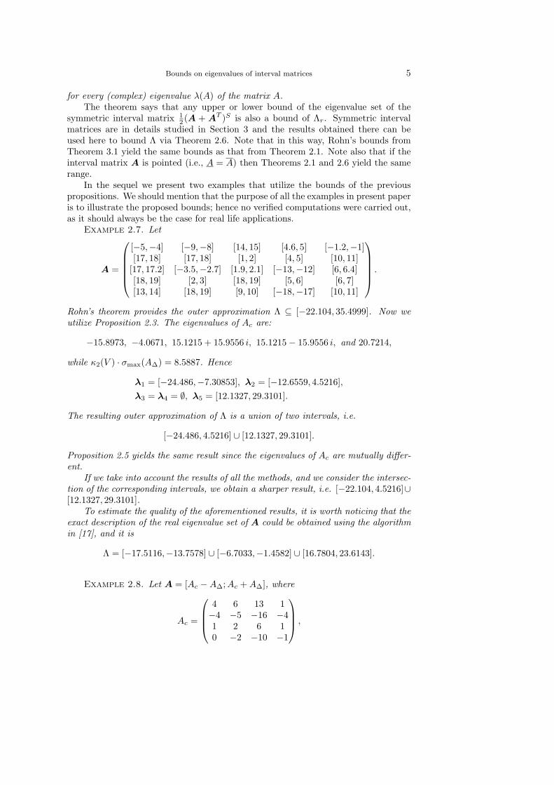
Example 2.7. Let

A =

[−5,−4] [−9,−8] [14, 15] [4.6, 5] [−1.2,−1][17, 18] [17, 18] [1, 2] [4, 5] [10, 11]

[17, 17.2] [−3.5,−2.7] [1.9, 2.1] [−13,−12] [6, 6.4][18, 19] [2, 3] [18, 19] [5, 6] [6, 7][13, 14] [18, 19] [9, 10] [−18,−17] [10, 11]

.

Rohn’s theorem provides the outer approximation Λ ⊆ [−22.104, 35.4999]. Now weutilize Proposition 2.3. The eigenvalues of Ac are:

−15.8973, −4.0671, 15.1215 + 15.9556 i, 15.1215 − 15.9556 i, and 20.7214,

while κ2(V ) · σmax(A∆) = 8.5887. Hence

λ1 = [−24.486,−7.30853], λ2 = [−12.6559, 4.5216],

λ3 = λ4 = ∅, λ5 = [12.1327, 29.3101].

The resulting outer approximation of Λ is a union of two intervals, i.e.

[−24.486, 4.5216] ∪ [12.1327, 29.3101].

Proposition 2.5 yields the same result since the eigenvalues of Ac are mutually differ-ent.

If we take into account the results of all the methods, and we consider the intersec-tion of the corresponding intervals, we obtain a sharper result, i.e. [−22.104, 4.5216]∪[12.1327, 29.3101].

To estimate the quality of the aforementioned results, it is worth noticing that theexact description of the real eigenvalue set of A could be obtained using the algorithmin [17], and it is

Λ = [−17.5116,−13.7578] ∪ [−6.7033,−1.4582] ∪ [16.7804, 23.6143].

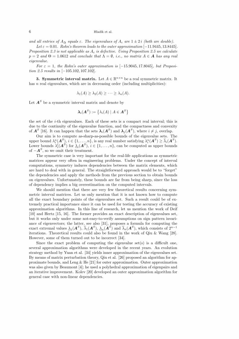
Example 2.8. Let A = [Ac − A∆;Ac + A∆], where

Ac =

4 6 13 1−4 −5 −16 −41 2 6 10 −2 −10 −1

,

6 Hladık et al.

and all entries of A∆ equals ε. The eigenvalues of Ac are 1 ± 2 i (both are double).

Let ε = 0.01. Rohn’s theorem leads to the outer approximation [−11.9445, 13.8445].Proposition 2.3 is not applicable as Ac is defective. Using Proposition 2.5 we calculatep = 2 and Θ = 1.0612 and conclude that Λ = ∅, i.e., no matrix A ∈ A has any realeigenvalue.

For ε = 1, the Rohn’s outer approximation is [−15.9045, 17.8045], but Proposi-tion 2.5 results in [−105.102, 107.102].

3. Symmetric interval matrix. Let A ∈ Rn×n be a real symmetric matrix. It

has n real eigenvalues, which are in decreasing order (including multiplicities):

λ1(A) ≥ λ2(A) ≥ · · · ≥ λn(A).

Let AS be a symmetric interval matrix and denote by

λi(AS) :=

{

λi(A) | A ∈ AS}

the set of the i-th eigenvalues. Each of these sets is a compact real interval; this isdue to the continuity of the eigenvalue function, and the compactness and convexityof A

S [16]. It can happen that the sets λi(AS) and λj(A

S), where i 6= j, overlap.

Our aim is to compute as-sharp-as-possible bounds of the eigenvalue sets. Theupper bound λu

i (AS), i ∈ {1, . . . , n}, is any real number satisfying λui (AS) ≥ λi(A

S).Lower bounds λl

i(AS) for λi(A

S), i ∈ {1, . . . , n}, can be computed as upper boundsof −A

S , so we omit their treatment.

The symmetric case is very important for the real-life applications as symmetricmatrices appear very often in engineering problems. Under the concept of intervalcomputations, symmetry induces dependencies between the matrix elements, whichare hard to deal with in general. The straightforward approach would be to “forget”the dependencies and apply the methods from the previous section to obtain boundson eigenvalues. Unfortunately, these bounds are far from being sharp, since the lossof dependency implies a big overestimation on the computed intervals.

We should mention that there are very few theoretical results concerning sym-metric interval matrices. Let us only mention that it is not known how to computeall the exact boundary points of the eigenvalues set. Such a result could be of ex-tremely practical importance since it can be used for testing the accuracy of existingapproximation algorithms. In this line of research, let us mention the work of Deif[10] and Hertz [15, 16]. The former provides an exact description of eigenvalues set,but it works only under some not-easy-to-verify assumptions on sign pattern invari-ance of eigenvectors; the latter, see also [31], proposes a formula for computing theexact extremal values λ1(A

S), λ1(AS), λn(AS) and λn(AS), which consists of 2n−1

iterations. Theoretical results could also be found in the work of Qiu & Wang [28].However, some of them turned out to be incorrect [34].

Since the exact problem of computing the eigenvalue set(s) is a difficult one,several approximation algorithms were developed in the recent years. An evolutionstrategy method by Yuan et al. [34] yields inner approximation of the eigenvalues set.By means of matrix perturbation theory, Qiu et al. [26] proposed an algorithm for ap-proximate bounds, and Leng & He [21] for outer approximation. Outer approximationwas also given by Beaumont [4]; he used a polyhedral approximation of eigenpairs andan iterative improvement. Kolev [20] developed an outer approximation algorithm forgeneral case with non-linear dependencies.

Bounds on eigenvalues of interval matrices 7

3.1. Basic bounds. The following theorem (without proof) appeared in [31];to make the paper self-contained, we present its proof.

Theorem 3.1. It holds that

λi(AS) ⊆ [λi(Ac) − ρ(A∆), λi(Ac) + ρ(A∆)].

Proof. By Weyl’s theorem [13, 18, 23, 33], for any symmetric matrices B,C ∈R

n×n it holds

λi(B) + λn(C) ≤ λi(B + C) ≤ λi(B) + λ1(C) ∀i = 1, . . . , n.

Particularly, for every A ∈ A in the form of A = Ac + A′, A′ ∈ [−A∆, A∆], we have

λi(A) = λi(Ac + A′) ≤ λi(Ac) + λ1(A′) ≤ λi(Ac) + ρ(A′) ∀i = 1, . . . , n.

As |A′| ≤ A∆, we get ρ(A′) ≤ ρ(A∆), whence

λi(A) ≤ λi(Ac) + ρ(A∆).

Working similarly, we can prove that λi(A) ≥ λi(Ac) − ρ(A∆).

The bounds obtained by the previous theorem are usually quite sharp. However,the main drawback is, that all the produced intervals λi(A

S), 1 ≤ i ≤ n, have thesame width.

The following proposition provides an upper bound for the largest eigenvalue ofA

S , that is an upper bound for the right endpoint of λ1(AS). Even though the

formula is very simple and the bound is not very sharp, there are cases that it yieldsbetter bound than the one by Rohn’s theorem. In particular it provides better boundsfor non-negative interval matrices, and for interval matrices as the ones we considerin Section 3.3 and have the form [−A∆, A∆].

Proposition 3.2. It holds

λ1(AS) ≤ λ1(|A|).

Proof. Using the well-known Courant–Fischer theorem [13, 18, 23, 33], we havefor every A ∈ A

λ1(A) = maxxT x=1

xT Ax ≤ maxxT x=1

|xT Ax|

≤ maxxT x=1

|x|T |A||x| ≤ maxxT x=1

|x|T |A||x|

= maxxT x=1

xT |A|x = λ1(|A|).

In the same way we can compute a lower bound for the eigenvalue set of A:λn(AS) ≥ −λ1(|A|). However, this inequality is not so useful in practice.

3.2. Interlacing approach, direct version. The approach that we propose inthis section is based on Cauchy’s interlacing property for eigenvalues of a symmetricmatrix [13, 18, 23, 33].

8 Hladık et al.

Theorem 3.3 (Interlacing property, Cauchy, 1829). Let A ∈ Rn be a symmetric

matrix and let Ai be a matrix obtained from A by removing the i-th row and column.Then

λ1(A) ≥ λ1(Ai) ≥ λ2(A) ≥ λ2(Ai) ≥ · · · ≥ λn−1(Ai) ≥ λn(A).

We develop two methods based on the interlacing property; the direct and theindirect one. These methods are useful as long as the intervals λi(A

S), i = 1, . . . , n,do overlap, or as long as there is a narrow gap between them. Overlapping happens,for example, when there are multiple eigenvalues in A

S . If none of the previous casesoccur, then the bounds are not so sharp; see Example 3.6.

The first method uses the interlacing property directly. Bounds on the eigenvaluesof the principal minor A

Si are also bounds on the eigenvalues of matrices in A

S

(except for λ1(AS) and λn(AS)). The basic idea is to compute the bounds recursively.

However, such a recursive algorithm would be of exponential complexity. Therefore,we propose a simple local search approach that requires only a linear number ofiterations and the results of which are quite satisfactory. It consists of selecting themost promising principal minor Ai and recursively using only this. To obtain evenbetter results in practice, we apply this procedure in the reverse order, as well. Thatis we begin with some diagonal element aii of A

S , which is a matrix one-by-one, anditeratively increase its dimension until we obtain A

S .

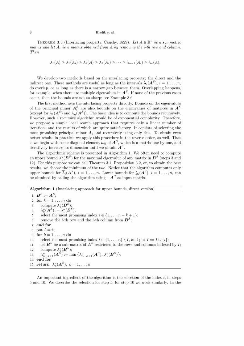
The algorithmic scheme is presented in Algorithm 1. We often need to computean upper bound λu

1 (BS) for the maximal eigenvalue of any matrix in BS (steps 3 and

12). For this purpose we can call Theorem 3.1, Proposition 3.2, or, to obtain the bestresults, we choose the minimum of the two. Notice that the algorithm computes onlyupper bounds for λi(A

S), i = 1, . . . , n. Lower bounds for λi(AS), i = 1, . . . , n, can

be obtained by calling the algorithm using −AS as input matrix.

Algorithm 1 (Interlacing approach for upper bounds, direct version)

1: BS := A

S ;2: for k = 1, . . . , n do

3: compute λu1 (BS);

4: λuk(AS) := λu

1 (BS);5: select the most promising index i ∈ {1, . . . , n − k + 1};6: remove the i-th row and the i-th column from B

S ;7: end for

8: put I = ∅;9: for k = 1, . . . , n do

10: select the most promising index i ∈ {1, . . . , n} \ I, and put I := I ∪ {i};11: let B

S be a sub-matrix of AS restricted to the rows and columns indexed by I;

12: compute λu1 (BS);

13: λun−k+1(A

S) := min{

λun−k+1(A

S), λu1 (BS)

}

;14: end for

15: return λuk(AS), k = 1, . . . , n.

An important ingredient of the algorithm is the selection of the index i, in steps5 and 10. We describe the selection for step 5; for step 10 we work similarly. In the

Bounds on eigenvalues of interval matrices 9

essence, there are two basic choices:

i := arg minj=1,...,n−k+1

λu1 (BS

j ), (3.1)

and

i := arg minj=1,...,n−k+1

∑

r,s 6=j

|Br,s|2. (3.2)

In both cases we select an index i so that to possibly minimize λ1(BSi ).

The first formula requires more computations than the second one, but yieldsthe optimal index in more cases than the second one. The latter is based on thewell-known result [18, 33] that the square of the Frobenius norm of a normal matrix(i.e., the sum of squares of its entries) equals the sum of squares of its eigenvalues.Therefore, the most promising index is the one that maximizes the sum of squares ofthe absolute values (magnitudes) of the removed components.

The selection rule (3.1) causes a quadratic time complexity of Algorithm 1 withrespect to the number of calculations of spectral radii or eigenvalues. Using theselection rule (3.2) results only a linear number of such calculations.

3.3. Interlacing approach, indirect version. The second method uses alsothe interlacing property, and is based on the following idea. Every matrix A ∈ A

S

can be written as A = Ac + Aδ with Aδ ∈ [−A∆, A∆]S . We compute the eigenvaluesof the real matrix Ac, and bounds on eigenvalues of matrices in [−A∆, A∆]S , and we“merge” them to obtain bounds on eigenvalues of matrices in A

S . For the “merging”step we use a theorem for perturbed eigenvalues.

The algorithm is presented in Algorithm 2. It returns only upper bounds λui (AS),

i = 1, . . . , n for λi(AS), i = 1, . . . , n, since lower bounds are computable likewise. The

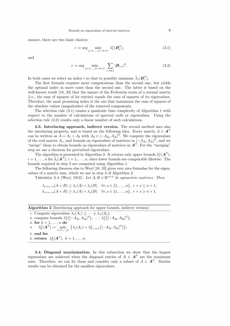
bounds required in step 2 are computed using Algorithm 1.The following theorem due to Weyl [18, 33] gives very nice formulae for the eigen-

values of a matrix sum, which we use in step 4 of Algorithm 2.Theorem 3.4 (Weyl, 1912). Let A,B ∈ R

n×n be symmetric matrices. Then

λr+s−1(A + B) ≤ λr(A) + λs(B) ∀r, s ∈ {1, . . . , n}, r + s ≤ n + 1,

λr+s−n(A + B) ≥ λr(A) + λs(B) ∀r, s ∈ {1, . . . , n}, r + s ≥ n + 1.

Algorithm 2 (Interlacing approach for upper bounds, indirect version)

1: Compute eigenvalues λ1(Ac) ≥ · · · ≥ λn(Ac);2: compute bounds λu

1

(

[−A∆, A∆]S)

, . . . , λun

(

[−A∆, A∆]S)

;3: for k = 1, . . . , n do

4: λuk(AS) := min

i=1,...,k

{

λi(Ac) + λuk−i+1

(

[−A∆, A∆]S)}

;

5: end for

6: return λuk(AS), k = 1, . . . , n.

3.4. Diagonal maximization. In this subsection we show that the largesteigenvalues are achieved when the diagonal entries of A ∈ A

S are the maximumones. Therefore, we can fix them and consider only a subset of A ∈ A

S . Similarresults can be obtained for the smallest eigenvalues.

10 Hladık et al.

Lemma 3.5. Let i ∈ {1, . . . , n}. Then there is some matrix A ∈ AS with diagonal

entries Aj,j = Aj,j such that λi(A) = λi(AS).

Proof. Let A′ ∈ AS be such that λi(A

′) = λi(AS). Such a matrix always exists,

since λi(AS) is defined as the maximum of a continuous function on a compact set.

We define A ∈ AS as follows: Aij := A′

ij if i 6= j, and Aij := Aij if i = j. By theCourant–Fischer theorem [13, 18, 23, 33], we have

λi(A′) = max

V ⊆Rn; dim V =imin

x∈V ; xT x=1xT A′x

≤ maxV ⊆Rn; dim V =i

minx∈V ; xT x=1

xT Ax

= λi(A).

Hence λi(A) = λi(A)′ = λi(AS).

This lemma implies that for computing upper bounds λui (AS) of λi(A

S), i =1, . . . , n, it suffices to consider only the symmetric interval matrix A

Sr ⊆ A

S definedas

ASr := {A ∈ A

S | Aj,j = Aj,j ∀j = 1, . . . , n}.

To this interval matrix we can apply all the algorithms developed in the previoussubsections. The resulting bounds are sometimes sharper and sometimes not so sharp;see Examples 3.6–3.7. So the best possible results are obtained by using all themethods together.

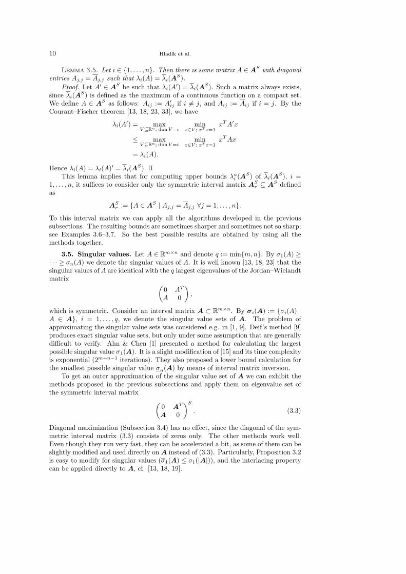
3.5. Singular values. Let A ∈ Rm×n and denote q := min{m,n}. By σ1(A) ≥

· · · ≥ σn(A) we denote the singular values of A. It is well known [13, 18, 23] that thesingular values of A are identical with the q largest eigenvalues of the Jordan–Wielandtmatrix

(

0 AT

A 0

)

,

which is symmetric. Consider an interval matrix A ⊂ Rm×n. By σi(A) := {σi(A) |

A ∈ A}, i = 1, . . . , q, we denote the singular value sets of A. The problem ofapproximating the singular value sets was considered e.g. in [1, 9]. Deif’s method [9]produces exact singular value sets, but only under some assumption that are generallydifficult to verify. Ahn & Chen [1] presented a method for calculating the largestpossible singular value σ1(A). It is a slight modification of [15] and its time complexityis exponential (2m+n−1 iterations). They also proposed a lower bound calculation forthe smallest possible singular value σn(A) by means of interval matrix inversion.

To get an outer approximation of the singular value set of A we can exhibit themethods proposed in the previous subsections and apply them on eigenvalue set ofthe symmetric interval matrix

(

0 AT

A 0

)S

. (3.3)

Diagonal maximization (Subsection 3.4) has no effect, since the diagonal of the sym-metric interval matrix (3.3) consists of zeros only. The other methods work well.Even though they run very fast, they can be accelerated a bit, as some of them can beslightly modified and used directly on A instead of (3.3). Particularly, Proposition 3.2is easy to modify for singular values (σ1(A) ≤ σ1(|A|)), and the interlacing propertycan be applied directly to A, cf. [13, 18, 19].

Bounds on eigenvalues of interval matrices 11

3.6. Case of study. The aim of the following examples is to show that nopresented method is better than the others. In different situations, different variantsare the best.

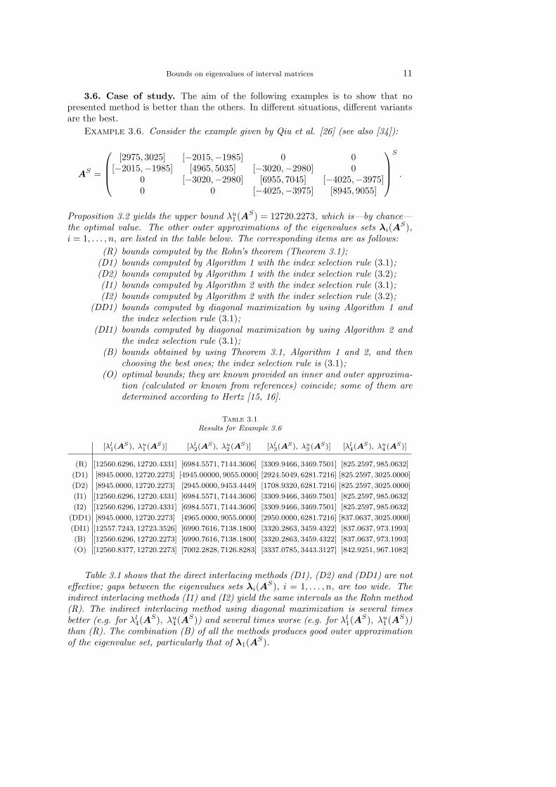
Example 3.6. Consider the example given by Qiu et al. [26] (see also [34]):

AS =

[2975, 3025] [−2015,−1985] 0 0[−2015,−1985] [4965, 5035] [−3020,−2980] 0

0 [−3020,−2980] [6955, 7045] [−4025,−3975]0 0 [−4025,−3975] [8945, 9055]

S

.

Proposition 3.2 yields the upper bound λu1 (AS) = 12720.2273, which is—by chance—

the optimal value. The other outer approximations of the eigenvalues sets λi(AS),

i = 1, . . . , n, are listed in the table below. The corresponding items are as follows:

(R) bounds computed by the Rohn’s theorem (Theorem 3.1);(D1) bounds computed by Algorithm 1 with the index selection rule (3.1);(D2) bounds computed by Algorithm 1 with the index selection rule (3.2);(I1) bounds computed by Algorithm 2 with the index selection rule (3.1);(I2) bounds computed by Algorithm 2 with the index selection rule (3.2);

(DD1) bounds computed by diagonal maximization by using Algorithm 1 andthe index selection rule (3.1);

(DI1) bounds computed by diagonal maximization by using Algorithm 2 andthe index selection rule (3.1);

(B) bounds obtained by using Theorem 3.1, Algorithm 1 and 2, and thenchoosing the best ones; the index selection rule is (3.1);

(O) optimal bounds; they are known provided an inner and outer approxima-tion (calculated or known from references) coincide; some of them aredetermined according to Hertz [15, 16].

Table 3.1Results for Example 3.6

[λl1(AS), λu

1(AS)] [λl

2(AS), λu

2(AS)] [λl

3(AS), λu

3(AS)] [λl

4(AS), λu

4(AS)]

(R) [12560.6296, 12720.4331] [6984.5571, 7144.3606] [3309.9466, 3469.7501] [825.2597, 985.0632]

(D1) [8945.0000, 12720.2273] [4945.00000, 9055.0000] [2924.5049, 6281.7216] [825.2597, 3025.0000]

(D2) [8945.0000, 12720.2273] [2945.0000, 9453.4449] [1708.9320, 6281.7216] [825.2597, 3025.0000]

(I1) [12560.6296, 12720.4331] [6984.5571, 7144.3606] [3309.9466, 3469.7501] [825.2597, 985.0632]

(I2) [12560.6296, 12720.4331] [6984.5571, 7144.3606] [3309.9466, 3469.7501] [825.2597, 985.0632]

(DD1) [8945.0000, 12720.2273] [4965.0000, 9055.0000] [2950.0000, 6281.7216] [837.0637, 3025.0000]

(DI1) [12557.7243, 12723.3526] [6990.7616, 7138.1800] [3320.2863, 3459.4322] [837.0637, 973.1993]

(B) [12560.6296, 12720.2273] [6990.7616, 7138.1800] [3320.2863, 3459.4322] [837.0637, 973.1993]

(O) [12560.8377, 12720.2273] [7002.2828, 7126.8283] [3337.0785, 3443.3127] [842.9251, 967.1082]

Table 3.1 shows that the direct interlacing methods (D1), (D2) and (DD1) are noteffective; gaps between the eigenvalues sets λi(A

S), i = 1, . . . , n, are too wide. Theindirect interlacing methods (I1) and (I2) yield the same intervals as the Rohn method(R). The indirect interlacing method using diagonal maximization is several timesbetter (e.g. for λl

4(AS), λu

4 (AS)) and several times worse (e.g. for λl1(A

S), λu1 (AS))

than (R). The combination (B) of all the methods produces good outer approximationof the eigenvalue set, particularly that of λ1(A

S).

12 Hladık et al.

For this example, Qiu et al. [26] obtained the approximate values

λ1(AS) ≈ 12588.29, λ1(A

S) ≈ 12692.77, λ2(AS) ≈ 7000.195, λ2(A

S) ≈ 7128.723,

λ3(AS) ≈ 3331.162, λ3(A

S) ≈ 3448.535, λ4(AS) ≈ 826.7372, λ4(A

S) ≈ 983.5858.

However, these values form neither inner nor outer approximation of the eigenvalueset. The method of Leng & He [21] based on matrix perturbation theory results inbounds

λl1(A

S) = 12550.53, λu1 (AS) = 12730.53, λl

2(AS) = 6974.459, λu

2 (AS) = 7154.459,

λl3(A

S) = 3299.848, λu3 (AS) = 3479.848, λl

4(AS) = 815.1615, λu

4 (AS) = 995.1615.

In comparison to (B), they are not so sharp. The evolution strategy method proposedby Yuan et al. [34] returns an inner approximation of the eigenvalues set, which isequal to the optimal result (see (O) in the table) in this example.

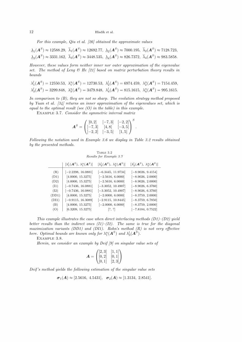
Example 3.7. Consider the symmetric interval matrix

AS =

[0, 2] [−7, 3] [−2, 2][−7, 3] [4, 8] [−3, 5][−2, 2] [−3, 5] [1, 5]

S

.

Following the notation used in Example 3.6 we display in Table 3.2 results obtainedby the presented methods.

Table 3.2Results for Example 3.7

[λl1(AS), λu

1(AS)] [λl

2(AS), λu

2(AS)] [λl

3(AS), λu

3(AS)]

(R) [−2.2298, 16.0881] [−6.3445, 11.9734] [−8.9026, 9.4154]

(D1) [4.0000, 15.3275] [−2.5616, 6.0000] [−8.9026, 2.0000]

(D2) [4.0000, 15.3275] [−2.5616, 6.0000] [−8.9026, 2.0000]

(I1) [−0.7436, 16.0881] [−3.3052, 10.4907] [−8.9026, 6.3760]

(I2) [−0.7436, 16.0881] [−3.3052, 10.4907] [−8.9026, 6.3760]

(DD1) [4.0000, 15.3275] [−2.0000, 6.0000] [−8.3759, 2.0000]

(DI1) [−0.9115, 16.3089] [−2.9115, 10.8445] [−8.3759, 6.7850]

(B) [4.0000, 15.3275] [−2.0000, 6.0000] [−8.3759, 2.0000]

(O) [6.3209, 15.3275] [?, ?] [−7.8184, 0.7522]

This example illustrates the case when direct interlacing methods (D1)–(D2) yieldbetter results than the indirect ones (I1)–(I2). The same is true for the diagonalmaximization variants (DD1) and (DI1). Rohn’s method (R) is not very effectivehere. Optimal bounds are known only for λu

1 (AS) and λl3(A

S).Example 3.8.Herein, we consider an example by Deif [9] on singular value sets of

A =

[2, 3] [1, 1][0, 2] [0, 1][0, 1] [2, 3]

Deif ’s method yields the following estimation of the singular value sets

σ1(A) ≈ [2.5616, 4.5431], σ2(A) ≈ [1.3134, 2.8541].

Bounds on eigenvalues of interval matrices 13

Ahn & Chen [1] confirmed that σ1(A) = 4.5431, but the real value of σ2(A) mustbe smaller. Namely, it is less or equal to one since σ2(A) = 1 for AT = ( 2 0 1

1 0 2 ).Our approach using combination of all presented methods together results in an outerapproximation

σ1(A) ⊆ [2.0489, 4.5431], σ2(A) ⊆ [0.4239, 3.1817].

4. Conclusion and future work. In this paper we considered outer approx-imations of the eigenvalue sets of general interval matrices and symmetric intervalmatrices. For both cases, we presented several improvements. Computing sharpouter approximations of the eigenvalue set of a general interval matrix is a difficultproblem. The proposed methods provide quite satisfactory results, as indicated byExamples 2.7–2.8. Examples 3.6–3.8 demonstrate that we are able to bound quitesharply the eigenvalues of symmetric interval matrices and the singular values of in-terval matrices. Our bounds are quite close to the optimal ones. Nevertheless, assuggested by one of the referees, it worths to explore the possibility to use a morenumerically stable decomposition than Jordan canonical form in Prop. 2.5.

At the current state, there is no algorithm that computes the best bounds in allthe cases. Since the computational cost of the presented algorithms is rather low, itis advisable to use all of them in practice and select the best one depending on theparticular instance.

5. Acknowledgments. The authors thank Andreas Frommer and the anony-mous referees for their valuable comments.

REFERENCES

[1] H.-S. Ahn and Y. Q. Chen. Exact maximum singular value calculation of an interval matrix.IEEE Trans. Autom. Control, 52(3):510–514, 2007.

[2] G. Alefeld and J. Herzberger. Introduction to interval computations. Academic Press, London,1983.

[3] G. Alefeld and G. Mayer. Interval analysis: Theory and applications. J. Comput. Appl. Math.,121(1-2):421–464, 2000.

[4] O. Beaumont. An algorithm for symmetric interval eigenvalue problem. Technical ReportIRISA-PI-00-1314, Institut de recherche en informatique et systemes aleatoires, Rennes,France, 2000.

[5] D. Chablat, P. Wenger, F. Majou, and J. Merlet. An interval analysis based study for the designand the comparison of 3-dof parallel kinematic machines. Int. J. Robot. Res., 23(6):615–624, 2004.

[6] K.-w. E. Chu. Generalization of the bauer-fike theorem. Numer. Math., 49(6):685–691, 1986.[7] K.-w. E. Chu. Perturbation theory and derivatives of matrix eigensystems. Appl. Math. Lett.,

1(4):343–346, 1988.[8] L. Cvetkovic, V. Kostic, and R. S. Varga. A new Gersgorin-type eigenvalue inclusion set.

ETNA, Electron. Trans. Numer. Anal., 18:73–80, 2004.[9] A. S. Deif. Singular values of an interval matrix. Linear Algebra Appl., 151:125–133, 1991.

[10] A. S. Deif. The interval eigenvalue problem. Z. Angew. Math. Mech., 71(1):61–64, 1991.[11] A. D. Dimarogonas. Interval analysis of vibrating systems. J. Sound Vib., 183(4):739–749,

1995.[12] F. Gioia and C. N. Lauro. Principal component analysis on interval data. Comput. Stat.,

21(2):343–363, 2006.[13] G. H. Golub and C. F. Van Loan. Matrix computations. 3rd ed. Johns Hopkins University

Press, 1996.[14] E. Hansen and G. W. Walster. Global optimization using interval analysis. 2nd ed., revised

and expanded. Marcel Dekker, New York, 2004.[15] D. Hertz. The extreme eigenvalues and stability of real symmetric interval matrices. IEEE

Trans. Autom. Control, 37(4):532–535, 1992.

14 Hladık et al.

[16] D. Hertz. Interval analysis: Eigenvalue bounds of interval matrices. In C. A. Floudas andP. M. Pardalos, editors, Encyclopedia of optimization., pages 1689–1696. Springer, NewYork, 2009.

[17] M. Hladık, D. Daney, and E. Tsigaridas. An algorithm for the real interval eigenvalue problem.Research Report RR-6680, INRIA, France, http://hal.inria.fr/inria-00329714/en/,October 2008. sumbitted to J. Comput. Appl. Math.

[18] R. A. Horn and C. R. Johnson. Matrix analysis. Cambridge University Press, Cambridge,1985.

[19] R. A. Horn and C. R. Johnson. Topics in matrix analysis. Cambridge University Press,Cambridge, 1994.

[20] L. V. Kolev. Outer interval solution of the eigenvalue problem under general form parametricdependencies. Reliab. Comput., 12(2):121–140, 2006.

[21] H. Leng and Z. He. Computing eigenvalue bounds of structures with uncertain-but-non-randomparameters by a method based on perturbation theory. Commun. Numer. Methods Eng.,23(11):973–982, 2007.

[22] H.-B. Li, T.-Z. Huang, and H. Li. Inclusion sets for singular values. Linear Algebra Appl.,428(8-9):2220–2235, 2008.

[23] C. D. Meyer. Matrix analysis and applied linear algebra. SIAM, Philadelphia, 2000.[24] A. Neumaier. Interval methods for systems of equations. Cambridge University Press, Cam-

bridge, 1990.[25] S. Poljak and J. Rohn. Checking robust nonsingularity is NP-hard. Math. Control Signals

Syst., 6(1):1–9, 1993.[26] Z. Qiu, S. Chen, and I. Elishakoff. Bounds of eigenvalues for structures with an interval

description of uncertain-but-non-random parameters. Chaos Solitons Fractals, 7(3):425–434, 1996.

[27] Z. Qiu, P. C. Muller, and A. Frommer. An approximate method for the standard intervaleigenvalue problem of real non-symmetric interval matrices. Commun. Numer. Methods

Eng., 17(4):239–251, 2001.[28] Z. Qiu and X. Wang. Solution theorems for the standard eigenvalue problem of structures with

uncertain-but-bounded parameters. J. Sound Vib., 282(1-2):381–399, 2005.[29] J. Rohn. Interval matrices: Singularity and real eigenvalues. SIAM J. Matrix Anal. Appl.,

14(1):82–91, 1993.[30] J. Rohn. Bounds on eigenvalues of interval matrices. ZAMM, Z. Angew. Math. Mech.,

78(Suppl. 3):S1049–S1050, 1998.[31] J. Rohn. A handbook of results on interval linear problems.

http://www.cs.cas.cz/rohn/handbook, 2005.[32] J. Rohn and A. Deif. On the range of eigenvalues of an interval matrix. Comput., 47(3-4):373–

377, 1992.[33] J. Wilkinson. The algebraic eigenvalue problem. 1. paperback ed. Clarendon Press, Oxford,

1988.[34] Q. Yuan, Z. He, and H. Leng. An evolution strategy method for computing eigenvalue bounds

of interval matrices. Appl. Math. Comput., 196(1):257–265, 2008.