P E R G A M O N

An Intematlonal Journal

computers & mathematics with applications

Computers and Mathematics with Applications 39 (2000) 1-15 www.elsevier, nl/locate/camwa

B o u n d s for S u m s o f E i g e n v a l u e s a n d A p p l i c a t i o n s

O . R O J O * AND m. S O T O Department of Mathematics, Universidad Cat61ica del Norte

Antofagasta, Chile

H . R O J O Department of Mathematics, Universidad de Antofagasta

Antofagasta, Chile

(Received November 1999; accepted December 1999)

A b s t r a c t - - L e t A be a matrix of order n × n with real spectrum A 1 ~ A2 ~_ " • • _~> A n . Let 1 < k < n - 2. If An or A1 is known, then we find an upper bound (respectively, lower bound) for the sum of the k-largest (respectively, k-smallest) remaining eigenwlues of A. Then, we obtain a majorization vector for (A1, A2,..., An-l) when An is known and a majorization vector for (A2, A3,..., An) when A1 is known. We apply these results to the eigenvalues of the Laplacian matrix of a graph and, in particular, a sufficient condition for a graph to be connected is given. Also, we derive an upper bound for the coefficient of ergodicity of a nonnegative matrix with real spectrum. (~) 2000 Elsevier Science Ltd. All rights reserved.

Keywords - -E igenva lues bounds, Laplacian matrix, Algebraic connectivity, Nonnegative matrices, Stochastic matrices, Coefficient of ergodicity.

1. I N T R O D U C T I O N

Let A be a mat r ix of order n × n with only real eigenvalues A1 :> A2 _> " • _> An.

In some impor tan t cases, An or A1 is known. For example, if A = L(G) , where L (G) is the Laplacian ma t r ix of a graph G, then An (G) = 0 and if A is a stochastic mat r ix with real

spec t rum, then A1 = 1.

It is well known tha t

A1 - - -

( ) u t ~ k ) + (A2 t r A ) + " ' + (An t r A ) = 0 ,

t r A ) 2 + (A 2 t r A ) 2 + . . . + (A n t ~ k ) 2 = tr ( A - t r A I ) 2

(An t r A ) 2 n - 1 [ ( t rA) 2] _< t r A 2 , n

(1)

(2)

(3)

Work supported by Fondecyt 1990363, Chile. *Part of this research was conducted while this author was a visitor at the International Centre for Theoretical Physics, Trieste, Italy.

0898-1221/00/$ - see front matter ~) 2000 Elsevier Science Ltd. All rights reserved. Typeset by ~.A/~S-TEX PII: S0898-1221 (00)00060-2

2 0. ROJO et al.

and

(4)

The equality in (3) occurs if only if Xr = Xp = . . . = X,.-l and the equality in (4) holds if and only X2 = As = ... = A,.

The above relationships suggest that we define the set

where a and b are real numbers satisfying the condition

a2 < n-l -b.

n

For each k, 1 5 k 5 n - 2, we define

f(x1,x2,.. .,x,-1)=z1+22+...+xlc.

We study the following optimization problems:

x = (X1,X2)

and

L(x,~)=f(x)+X~(2~+22+~~~+~~_l+a)+~~(x~+~~+~~.+x~_~+~2-b).

We search for the stationary points of L. We have

$x,X) = 1+ x1 + 2X22i = 0, i=1,2 ,..., k, 2

$x,X) = x1 + 2X2Zci = 0, Z

i=k+l,...,n-1.

Thus, we obtain

Xl = 22 = . . . = Xk and 2&+1 = 2,++2 = ... = X,-l.

Let x = (XI, a+7 xl, xk+l, . . . , xk+l) E s. Then,

kxl + (n k - l)xk+l =

kxy + (n - k - ~)xZ+~ = b - u2.

Then,

This equation becomes

kx2 + (kxl + aI2 1 n-k-l

+ a2 - b = 0.

(5)

(6)

(7)

k (n - 1) x2 + 2ka n- k

n-k-l ’ n-k-l Xl +

n-k-l a2-b=O

Eigenvalues and Appl i ca t ions 3

and its roots are

o n ] = n - - 1 V kT -U b - i , (s)

and

l k - - n - - 1 + v - k - ( n - - - - ] ) b - n - 1 a2 " (9)

By condition (5) on the numbers a and b, it follows tha t sk and lk are real numbers and - - a

sk < < lk. (10) n - 1

Therefore, if (xl, x 2 , . . . , xn-1) is a s tat ionary point of Lagrangian L, then

X 1 : X 2 : ' ' • : X k : 8 k and

and

Xl : x 2 . . . . . xk : Ik and

The Hessian of both optimization problems is

From (6) and (7), we obtain

Let xl = sk. Then, by (10),

- a - k s k (11) • • - ~ X n - 1 - - n _ k _ 1

- a - k l k • = X n - 1 - n - k - l " ( 1 2 )

2$k_F1 : Xk_l_ 2 :

Xk+ 1 : Xk+ 2 :

V2L(x, A) = 2A2I.

1 + 2A2 (xl - Xk+l) = 0.

- a - k x l - a + k a / ( n - 1)

n - k - 1 n - k - 1

- a

X k + l - n - 1 > x l "

(13)

Hence, xl - xk+l < 0 and, from (13), A2 > 0. Therefore, •2L(x, A) -- 2A2I is a positive definite

matrix. Thus, f at tains a minimum at x given by (11) and fmin : k8k" NOW, let Xl = lk.

By (10), - a - k x l - a + k a / ( n - 1) - a

Xk+l = n - k - 1 < - < x l . n - k - 1 n - 1

Hence, x l - xk+l > 0 in (13) and then A2 < 0. Therefore, V2L(x *,~k) = 2A2I is a negative

definite matrix. Thus, by choosing xl = lk, f at tains its maximum value at x given by (12) and

fmax = k lk . Thus, we have proved the following theorem.

THEOREM 1. L e t a and b be real numbers s a t i s f y i n g the c o n d i t i o n a 2 < (n - 1 / n ) b . L e t

S = { ( X l , X 2 , . . . , X n - 1 ) E R n - 1 ' X l + x 2 W " ' - F X n - l H - a = O , } x2 + x2 + " " + X2n-1 + a 2 = b

L e t 1 < k < n - 2 a n d

f ( X l , X 2 , . . . , a n - l ) : Xl -F X2 - F " " "F Xk.

Then, f (x) = ksk f (x) : k k,

sk and Ik are g i v e n b y (8) and (9), r e s p e c t i v e l y .

Theorem 1 is the fundamental theorem for the results of this paper. The rest of the paper is organized as follows• In Section 2, we assume that A is a matr ix of order n x n with real spec t rum A1 _> A2 _> . . . _> An. For each 1 < k <_ n - 2 , if An or A1 is known, we find an upper bound (respectively, lower bound) for the sum of the k-largest (respectively, k-smallest)

remaining eigenvalues of A. Then we obtain a majorization vector for (A1, A2,. • •, An-l ) when An is known and a majorization vector for (A2, A3, . . . , An) when A1 is known• In particular, k = 1 yields to an interval containing all .the remaining eigenvalues. In Section 3, we apply the results of Section 2 to derive an upper bound for the largest eigenvalue and a lower bound for the second smallest eigenvalue of the Laplacian matr ix of a graph• In particular, a sufficient condition for a graph to be connected is given. Section 4 is devoted to finding an upper bound for the coefficient of ergodicity of a nonnegative matr ix with real spectrum.

4 O. ROJO et al.

2. B O U N D S F O R S U M S O F E I G E N V A L U E S

Let A be a matrix of order n × n with only real eigenvalues A1 _> A2 _> . . . _> An. We mention some interesting cases of such a matrix A.

1. A is the Laplacian matrix of a graph. 2. A is a stochastic symmetric matrix. 3. A is a diagonally symmetrizable matrix, that is, A = D-1C for some diagonal matrix D

with positive diagonal entries and a nonnegative irreducible symmetric matrix C.

We assume that An is known. Our purpose now is to apply Theorem 1 to A in order to get some information about the remaining eigenvalues.

THEOREM 2. Let A be an n x n matrix with only real eigenvalues A1 _> A2 _> .. • _> An. Suppose that An is known. Let 1 < k < n - 2. Then,

A1 + A2 + . - . + Ak _< bk (14)

and

where

and

ak ~_ A n - 1 q- A n - 2 q- " ' " q- A n - k , ( 1 5 )

k (trA - An) I k (n - k - 1) bk -- n - 1 q- n'---T f ( A ) , (16)

k (trA - An) I k (n - k - I ) ak = f (A), (17) n - 1 n - 1

( r A ) 2 ( t r A ) 2 f ( A ) = t r A - - - t I n An - • (18)

n - 1

PROOF. Let a = A n - t r A / n and b = t r ( A - ( trA/n)I) 2. By (3), a 2 ~ (n -1 /n )b . I f a 2 = (n - 1/n)b, then A1 = A2 . . . . . A,-I = (trA - An/n - 1) and f (A) = 0. Thus, the equality holds in both inequalities (14) and (15). Hence, we assume that a 2 < (n - 1/n)b. Let S be as in Theorem 1. The roots sk and lk are

( t r A / n ) - A n i n - k - 1 [ ( t r ~ t ) 2 n (An e rA) 2] s k - n - 1 k~n--''l) A - ,o I ?2 1

and

( t r A / n ) _ A n i n _ k _ l [ ( ~_A )2 ( t r A ) 2 ] lk = n 1 + k ( n - 1) tr A - I n An

- n - 1 "

From (1) and (2), for a = An - t r A / n in Theorem 1, we have

trA A1 n

and t rA

An--1 n

Thus, from Theorem 1, we obtain

m g f (x) = klk

IAI-_

. . . . , . . . ,An-1 E $ ?2

t rA ,A1 t r A ) E S. - - - - . . - -

-- - - ~ )~n-2 ?2 '" ?2

t ~ ) ÷ (A2 t_~A) _b... ÷ (Ak t~A) (19)

Eigenvalues and Applications 5

and f (x) = ksk

-< ( A n - l - t r A ) + ( A ' ~ - 2 n t r A ) + ' " + ( An-k t r A ) . (20)

Now, from (19) and (20), inequalities (14) and (15) are immediate. |

In particular, for k = 1 in Theorem 1, we have the following.

COROLLARY 3. Let A bean n x n matrix with only real eigengalues A1 >_ A2 >_ . . . >_ An. Suppose that )% is known. Then,

AI_< t r A - An In--~_21f(A) n - 1 + (21)

and t rA - An ~/n - 2

n - 1 ~ _ l f (A) < An-l, (22)

where f ( A ) is given by (18).

We observe that (21) and(22) define an interval containing the eigenvalues A1, A2, . . . , An-1.

Since

and

tr A - t - - - - I = t r ( A 2) n

i= l k=l

the bounds given in Theorem 2 and Corollary 3 can be computed without squaring the matrix A. In particular, if A is a Hermitian matrix, then t r (A 2) = ]]AI] ~, where ]]AIIF is the Frobenius

matrix norm of A. We observe that for k = n - 1, the equality holds in both (14) and (15). In fact, A1 + A2 +

• " + An-1 = bn-1 = an-1 = t rA - An. We define bo = 0. Let us consider the sequence

bl - b o , b 2 - b l , b a - b 2 , . . . , b n - 1 - bn-2. (23)

In order to prove that (23) is decreasing, we need the following lemma whose proof is straight-

forward.

LEMMA 4. H a >_ 1 and fl >_ 1, then

2V/-~ _ X/(a + 1) (fl - 1) ÷ X/(a - 1) (fl + 1). (24)

Let 1 < k < n - 2. From Lemma 4, we obtain

2k ( t rA - An) 2bk

n - 1

2k ( t rA - An) > - n - 1 = b k + l + b k - ~ .

+ 2 x / k ( n - k - 1 ) I n 1 - ~ _ 1 f (A)

+ ( v / ( k ÷ l ) ( n - k - 2 ) + v / ( k - 1 ) ( n - k ) ) ~ (A)

Therefore, for 1 < k < n - 2, we have bk -- bk -1 ~_ bk+l - bk. We have proved the lemma.

6 O. RoJo et al.

LEMMA 5.

bl >_ b2 - bl >_ b3 - b2 >_ " . >_ b ,~- i - b n - 2 .

We recall the not ion of major iza t ion [1]. Given two m-dimensional real vectors x and y , the

vector y majorizes the vector x if the sum of the k largest entries of y is greater than or equal

to the sum of the k largest entries of x for k = 1, 2 . . . . , m - 1 and the sums of the entries of y and x are equal.

COROLLARY 6. L e t A b e a n n x n matr /x w i t h o n l y r e a l e i g e n v a l u e s A1 _> A2 _> .. • > An. S u p p o s e

t h a t An i s k n o w n . T h e n the v e c t o r

b - - (bl,b2 - bl , ba - b2 , . . . , b n - 1 - b n - 2 )

m a j o r i z e s t h e v e c t o r A = (A1, A2, A3 , . . . , "~n--1). PROOF. From (14) , for 1 < k < n - 2 ,

Moreover,

k-1

)~1 -{- )~2 -[- ' ' " ~- )~k <-- bk = ~ ( b j + l - b j ) .

j=O (25)

n-2

.~1 -[- )~2 -[- ' ' " -[- A n - 1 = bn-1 -- Z (b j+l - b j ) . (26) j=0

Since A1 _> A2 _> ".. _> An-1 and bl >_ b2 - bl _> b3 - b2 _> . . . _> b n - 1 - b n - 2 , (25) and (26) show t h a t the vector b majorizes the vector of eigenvalues A. |

In the examples in this paper, the results will be rounded to two decimal places.

EXAMPLE 7. Let } ] - 1 5 - 2 - 1 - A ---- - 2 - 2 8 - 2 - .

7 -

- 1

A5 = 0 is its smallest eigenvalue. From

- 3 - 1 - 2

0 - 1 - 2

Clearly, A is a positive semidefinite mat r ix and

T h e o r e m 2, we have the following.

k ak Lower Bound For

1 3.35 A4

2 10.20 A4 -b A3

3 18.35 A4 -4- A3 -{- A2

k bk Upper Bound For

1 11.65 AI

2 19.80 A1 + A2

3 26.65 A1 + A2 q- A3

The eigenvalues of A are 0, 4.354249, 6, 9.645751, and I0.

Now, let A be an n x n matrix with nonnegative eigenvalues A1 >_ A2 >_ .-. _> An. We define the (n + 1) x (n + 1) mat r ix

0] T h e eigenvalues of B are

A1 _> A2 _> " . >_ AN and 0.

Since 0 is the smallest eigenvalue of B, we can apply Theorem 2 to B to obta in the following.

EigenvMues and Applications 7

THEOREM 8. Let A be an n x n matr/x with nonnegative eigenvalues

A, >_ A2 >_ . . . >_ An.

Let l < k < n - 1 . Then,

and

where

A 1 "4- A2 "~- " " ' + Ak ---~ ~k

ak _< An + An-t + ' " + An-k+1,

(27)

(28)

and

~k - ktrAn + i k(nn- k) f (A)' (29)

k t r A ~/k(n - k) / (A), (30) Ol k --

n n

n

f (A) ---- E aikaki (trA)2 (31) n

i = 1 k----1

In particular,

REMARK 1. We observe the following.

1. If n n

(trA) 2 > ( n - 1) E E aikaki, i = 1 k----1

then the lower bound (~1 for An is positive, and thus, the eigenvalues of A are positive. 2. We can apply Theorem 8 to a positive semidefinite matrix A and, in this case, ~n__ 1 ~ k = l

aikaki = IIA{I~.

EXAMPLE 9. Let

6 -1 -1 -2 - i l - 1 5 - 1 0 A = - 1 - 1 4 - 1 - .

- 2 0 - 1 3 - 1 2 - 1 0

From the Gerschgorin Theorem, we see that the eigenvalues of A lie in the interval [0, 11]. Hence, the eigenvalues of A are nonnegative numbers, and thus, we can apply Theorem 8 to obtain the following.

c~ k Lower Bound For

0.24 A5

4.32 As -b A4 9.52 A5 + )~4 + A3

3.96 A5 + A4 "~ A3 + A2

k ~k Upper Bound For 1 10.16 )~1

2 16.48 A1 "{- A2

3 21.68 A1 -{- A2 "4- A3

4 2 5 . 7 6 A1 -{" A2 "}- A3 "}- A4

Suppose now that )~1 is known. Let a = A1 - t r A / n and b = tr (A - ( t rA /n ) I ) 2. Similarly, from Theorem 1 and Lemma 4, the following theorem and corollaries can be derived.

8 0. ROJO et al.

THEOREM 10.

that A1 is known. Let 1 < k < n - 2. Then,

A2 -~- A3 -[- " '" -~- Ak+l ~ dk

and

where

and

Let A be an n x n matrix with only real eigenvalues A1 _> A2 _> . . . _> An. Suppose

(32)

d k -~

O k - -

Ck _< An + An-1 + . . . + An-k+1, (33)

k ( t rA - A1) ~/k (n-yk___- 1) n - 1 + V n - 1 f (A), (34)

k ( t rA - A1) ~ / k ( n _ - - k - 1) n - 1 Y n - 1 f (A), (35)

f ( A ) = t r A - I n A1 • (36) n 1

COROLLARY 11.

Suppose that A1 is known. Then, Let A be an n x n matrix with only real eigenvalues A1 _> A2 _> . . . _> An.

and

where f (A) is given by (36).

t r A - A 1 ~/n-~_ 12f (A) A2 ~_ dl - n-----Z-i-- + (37)

t r A - A1

n - 1 ~n - 2 f A ( ) = e l ___ A n , (38)

COROLLARY 12. Let A be an n x n matrix with only real eigenvMues A1 _> A2 >_ . . - _> An. Suppose that A1 is known. Then the vector

(d,, d2 - dl, d3 - d2 , . . . , dn-1 - dn-2)

majorizes the vector (A2, A3, . . . , An). Here, dn-1 = t rA - A1.

We observe tha t (37) and (38) define an interval containing the eigenvalues A2, A3, . . . , An. As before, we observe tha t the bounds given in Theorem 10 and Corollary 11 can be computed

without squaring the matr ix A.

EXAMPLE 13. Let 0.09 0.1 0.6 0.11 0.1 0.1 0 0.3 0.4 0.2

A = 0.6 0.3 0.025 0.025 0.05 0.11 0.4 0.025 0.375 0.09

10.1 0.2 0.05 0.09 0.56

This matr ix is stochastic and symmetric. From Theorem 10, we have the following.

Then, its eigenvalues are real numbers and A1 = 1.

k ck Lower Bound For

1 -0.79 A5

2 -0.90 A5 + A4

3 -0.76 A5 -{- A4 ~- A3

k dk Upper Bound For

1 0.81 A2

2 0.95 A2 + A3

3 0.83 A2 + A3 + A4

The eigenvalues of A are -0.623486, -0.226595, 0.402888, 0.497193, and I.

Eigenvalues and Applications 9

3. A P P L I C A T I O N T O T H E L A P L A C I A N G R A P H E I G E N V A L U E S

Let G = (V,E) be a nonempty graph on n vertices vl,v2,... ,vn. Let d(v) be the degree of v E V. Let A(G) be the adjacency matrix of G and let D(G) = diag{d(Vl),d(v2 ), . . . ,d(vn)}. The Laplacian matrix of G is defined as L(G) = D(G) - A(G). The matrix L(G) is clearly a real symmetric matrix. From this fact and Ger~gorin's Theorem, it follows that its eigenvalues are nonnegative real numbers. Moreover, since its rows sum to 0, 0 is the smallest eigenvalue of

L(G). In this section, AI(G) ~_ A2(G) ~_ - " ~_ An(G) = 0 are the eigenvalues L(G). Clearly,

n

tr (L (G)) = Z d (v~) i=1

and n

tr (L 2 (G)) ---- E d ( v , ) ( d ( v i ) + 1). i---1

We apply Theorem 2 to L (G) to obtain the following.

THEOREM 14. If G is a graph on n vertices, then [or each 1 < k < n - 2,

~1 ( G ) + ~2 ( G ) -~- • . • -~-/~k (G) _< bk ( G ) (39)

and ~k (a) <_ ~,.-1 (a) + a~-2 (a) + . . . + a~-k ( a ) , (40)

where

k ~ d (v~) bk (G) - ~=1 + ~ / k ( n - k - 1 )

n - 1 V n'-"l" f ( G ) , (41) n

kE (v,) ,/k(n-k- ak(G) -- ~=1 (42) n - 1 V n-'--i 1) f (G),

and

n Vi

f (V) = E d (vi) (d (vi) + 1) - (43) n - 1

i=1

EXAMPLE 15. Let G be the graph on V -- {1,2,3,4,5,6,7,8} with edge set

E - - { {1 ,6} ,{1 ,2} ,{3 ,7} ,{7 ,8} ,{1 ,4} ,{1 ,7} ,{2 ,3} ,{3 ,4} , {4, 5}, {5, 6}, {6, 7}, {2, 6}, {5, 8}, {4, 8} }"

From Theorem 14, we have the following.

] Lower k ak Bound For

1 0.30 A7 (G)

2 3.22 E~=~ ~-J (a) 3 6.76 Z3=~ ~_j (G)

4 10 .76 E~fI~8-~(G) 5 15.22 5

e 6 20.30 ~-~j=l AS--J (G)

Upper bk Bound For

7.70 Ax (G)

12.7s E~=~ ~ (a) 17.24 ~"~ffil AJ (G)

21.24 )"~4=i Aj (G)

24.7s E~=~ ~J (a) 6 27.70 5-~.jffi 1 Aj (G)

From Theorem 14, for k = 1, we have the following corollary.

10 O. RoJo et al.

COROLLARY 16. I f G is a graph on n vertices, then

f i d (vi) i = 1 _ _ / n - 2

AI(G)<_ n - 1 + V ~ - ~ _ l f ( C ) (44)

and n

E d (vi) i=1 ~ /n - 2

n - 1 V n - 1 f (G) < An-1 (G), (45)

with f ( a ) given by (43).

In (44), we have an upper bound for AI(G). Before giving an example concerning the upper bounds for AI(G), we list some others known bounds for A1.

ANDERSON AND MORLEY'S BOUND. (See [2].)

~1 ~ max {d (u) + d (v) : uv E E } . (46)

LI AND ZHANG'S BOUND. of G, then

MERRIS'S BOUND. then

(See [3].) If dl >_ d2 >_ d3 >_ . . . >_ dn are the degrees of the vertices

A1 _( 2 + v/(dl + d2 - 2) (dl + d3 - 2). (47)

(See [4].) If m(v) is the average of the degrees of the vertices adjacent to v,

A1 _< max{d(v) + m ( v ) : v e V}. (48)

OTHER LI AND ZHANG'S BOUND. (See [3].) If r is the right-hand side of (46), and xy E E is such that d(x) + d(y) = r and if s = max{d(u) + d(v) : uv E E - {xy}}, then

)~1 ---~ 2 Je 4(?" -- 2)(S -- 2). (49)

The bounds (47)-(49) are better than (46). In [4], the author gives examples which show that (48) and (49) are incomparable. However, the author observes that (48) is usually the better bound.

A NEW LI AND ZHANG'S BOUND. (See [5].)

{ d ~ ( d u + m ~ ) + d v ( d v + m v ) } )u <_max du + dv : uv E V . (50)

In [5], the authors prove that (50) is better than (48).

EXAMPLE 17. For the graph considered in Example 15, AI(G) = 6.43 and the use of (44) give A1 (G) < bl = 7.70, which is better than the bounds obtained by the use of (46)-(49).

i ,,0, i i i ,49, r ,50, I 8.00 8.00 8.00 7.75 7.63

EXAMPLE 18. Let G be the graph on V = {1, 2, 3, 4, 5, 6, 7, 8, 9, 10} with edge set

E : ~ {3, 4}, {i, 5}, {I, 4}, {I, 9}, {I, I0}, {I, 7}, {2, 6}, {8, 9}, I ( (1, S} ,{5 ,10} ,{1 ,2} ,{1 ,3} ~

For this graph, A1 (G) = 9.02, bl -- 9.59, and the following.

i i [ 48, ,40, i 50, q I0.00 i0.00 i0.00 9.88 9.78

Eigenvalues and Applications 11

Of course, there are graphs for which the bounds given in (46)-(50) give better estimates than

bl does. Further information given by Corollary 16 in (45) is a lower bound for A~-I(G). This lower

bound is al(G). In [2], it is proved that the multiplicity of An(G) = 0 is equal to the number of connected component of G. Then, G is a connected graph if and only if A~_I(G) ~ 0. Because of this fact, An-I(G) is called the algebraic connectivity of G. In [6], this concept is discussed, together with some of its applications. A sufficient condition for a graph to be connected is given in the next corollary.

COROLLARY 19. If

(n - 2) ~,_.., d (vi) (d (vi) + 1) < d (vi) , (51) i = l i=1

the graph G is connected.

PROOF. One can easily prove that the lower bound for £~-I(G) in (45) is positive if and only if the inequality in (51) holds. |

EXAMPLE 20. For the graph in Example 15, we have al(G) = 0.30.

4. A N U P P E R B O U N D F O R T H E C O E F F I C I E N T

O F E R G O D I C I T Y

If A is a nonnegative matrix of order n × n, then by the Perron-Frobenius Theorem, A has a real eigenvalue equal to its spectral radius p(A). This eigenvalue is usually denoted by r(A) and it is called the Perron root of A. An eigenvalue of A which is different from r(A) is called a subdominant eigenvalue of A. Localization theorems for the subdominant eigenvalues of A have been studied by several authors and special attention has been devoted to find upper bounds for the maximum modulus of the subdominant eigenvalues of A. This maximum modulus is called the coefficient of ergodicity of A and it is denoted by ~(A). Upper bounds for ~(A) are important because ~(A) plays a major role in convergence properties of powers of A. The upper bounds for ~(A) are usually given in terms of r(A).

In this section, we suppose that A is a nonnegative matrix for order n x n matrix with real eigenvalues

r (A) = ~1 > ~2 > "'" > ~ ,

and that r (A) is known. An example of such a matrix A is given by a stochastic symmetric matrix.

Our purpose in this section is to find an upper bound for ~(A). We have

(A) = max {[A,~[, [A21}-

From Corollary 11,

and

where

t r A - r ( A ) I n - ~ _ 2 1 f C 1 ~--- ( A ) < /~n (52) n - 1

t r A - r (A) / n - 2 A2 <_ dl - 1 + 1 f ( A ) , ( 5 3 )

f (A) tr A t I n = - - - . n - 1

( 5 4 )

12

THEOREM 21.

Then,

O. RoJo et al.

Let A be an n x n noanegative matrix with only real eigenvalues

AI ~__ A2 ~__ "'" ~__ An.

(A) < max{-Cl ,d l} ,

where cl and dl are given in (52) and (53), respectively.

PROOF. If A2 < 0, then An < 0, and thus,

(A) = - A n __~ --C 1.

Hence, if As _< 0, then (55) holds. Suppose As > 0. Now, An > 0 or An _< 0. If An > 0, then

(A) = A2 < dl,

and thus, (55) holds. Finally, if An < 0, then

( A ) = - A n _~ --Cl or ~ (A) = A2 _< d l ,

and therefore, (55) also holds.

EXAMPLE 22. Let us consider again the matrix of Example 13,

0.09 0.1 0.6 0.11 0.1 ] 0.1 0 0.3 0.4 0.2

A = 0.6 0.3 0.025 0.025 0.05 . 0.11 0.4 0.025 0.375 0.09|

10.1 0.2 0.05 0.09 0.56J

In Example 13, we got

Therefore,

Cl = -0.79 < A5 and A2 ~ dl = 0.81.

(55)

|

Then,

is a positive eigenvector of A corresponding to r(A). Some of these bounds are as follows.

1. Let

m j = min ~a~j~ and M j = max ~ a i j ~ . x<_i<_n I wi J l < i < n ~, Wi J

{ ° o } ~(A)_<min r ( A ) - Z w j m j , Z w j M j - r ( A ) .

j=l i=1

This bound is a modified version of a result due to Hoffman for stochastic matrices [8].

(56)

w = [Wl, w 2 , . . . , wn] T

(A) < 0.81.

The exact coefficient of ergodicity rounded to two decimals is 0.62.

Now, we want to compare our upper bound for the coefficient of ergodicity with other known upper bounds. We recall some of them.

In [7], the authors give a unified presentation of results concerning upper bounds on ~ (A) for a nonnegative irreducible A. Here

Eigenvalues and Applications 13

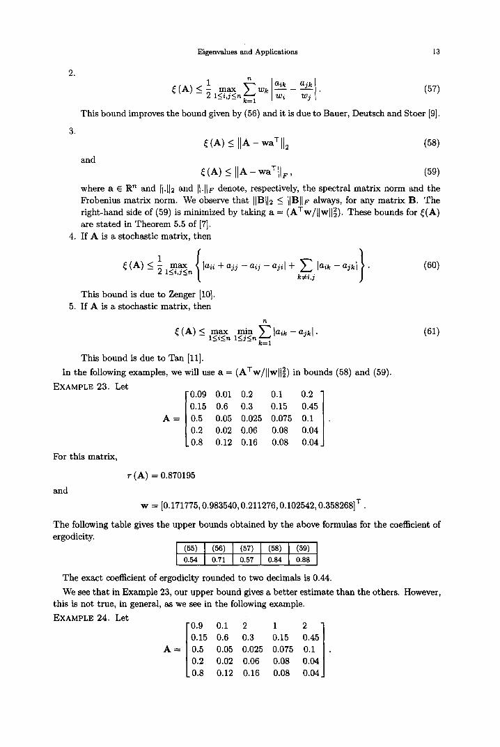
2.

.

1 max 3-" wk ajk (57) (A) _< ~ a<_i , j<_n~ w i w j "

This bound improves the bound given by (56) and it is due to Bauer, Deutsch and Stoer [9].

and

~(A) < IIA- waTl]2 (58)

(A) <_ IIA - wa-vllF, (59)

where a e R '~ and 11.[[2 and II.IIF denote, respectively, the spectral matrix norm and the Frobenius matrix norm. We observe that IIBII2 _< IIBIIF always, for any matrix B. The right-hand side of (59) is minimized by taking a = (ATw/HwlI~). These bounds for ~(A) are stated in Theorem 5.5 of [7].

4. If A is a stochastic matrix, then

~(A) < max lai~. + a j j - aj~l + ~ la~k - a jk l • (60) - l_<id_<n

This bound is due to Zenger [10]. 5. If A is a stochastic matrix, then

n

(A) < max min ~ l a ~ k - - a j k [ . (61) l < i < n . . . . l < j < n ~ = 1=

This bound is due to Tan [11].

In the following examples, we will use a -- ( h r w / l l w l l ~ ) in bounds (58) and (59).

EXAMPLE 23. Let

For this matrix,

A =

and

0.09 0.01 0.2 0.1 0.2 0.15 0.6 0.3 0.15 0.45 0.5 0.05 0.025 0.075 0.1 0.2 0.02 0.06 0.08 0.04 0.8 0.12 0.16 0.08 0.04

r (A) = 0.870195

w = [0.171775, 0.983540, 0.211276, 0.102542, 0.358268] T .

The following table gives the upper bounds obtained by the above formulas for the coefficient of ergodicity.

0.54 0.71 0.57 0.84 0.88

The exact coefficient of ergodicity rounded to two decimals is 0.44.

We see that in Example 23, our upper bound gives a better estimate than the others. However,

this is not true, in general, as we see in the following example.

EXAMPLE 24. Let

A = I 0.9 0.1 2 1 2 1

0.15 0.6 0.3 0.15 0.45 0.5 0.05 0.025 0.075 0.1 [ . 0.2 0.02 0.06 0.08 0.04 0.8 0.12 0.16 0.08 0.04J

14

For this matrix,

and

O. RoJo et al.

r (A) = 2.298704

w ---- [0.920540, 0.224563, 0.226310, 0.097569, 0.357459] x

The upper bounds for ~ (A) given by the above formulas are as follows.

1.26 1.57 1.45 1.20 1.34

The exact coefficient of ergodicity rounded to two decimals is 1.17.

We finish with an example for a stochastic matrix.

E X A M P L E 2 5 . L e t '0.2 0.01 0.46 0.01 0.32 ] 0.01 0 0.3 0.4 0.29 [

/

A = 0.46 0.3 0.2 0.025 0.015[ . /0.01 0.4 0.025 0.37 0.195 / !

L032 029 0.015 0.195 0 1 8 j

Clearly, r (A) -- 1 and w -- [1, 1, 1, 1, 1] T. The upper bounds for ~(A) are as follows.

0.70 0.95 0.75 0.55 0.79 0.75 0.78

We observe that in Example 25, the bound given by (58) coincides with the coefficient of ergodicity. It is true, in general, that if _A. is a symmetric irreducible nonnegative matrix, then

d A ) = A - r (A) wwT Ilwll~ 5" (62)

In fact, Brauer [12] proved that for every vector a E R n, the eigenvalues of A and A - wa T coincide except tha t the eigenvalue r (A) is replaced by r (A) - aXw. Then,

(A) _< p (A - wa T)

= max { [r (A) - aTw [ , [AS[, [z~3],..., [ / ~ n [ } •

For a = (ATw/llwll~), we have

r (A) - a T w ---- r (A)

Hence, by selecting a - ( A T w / l l w l h 2 ) ,

w T A w Ilwll2 2 - r (A) - r (A) = 0.

w T A ~ ~ ( A ) = p A-w-~-~, ,2 . Ilwl12)

Finally, taking into account that A is a symmetric matrix, we have

~(A) = p []w[[2 ]

w w T w w T

However, when evaluating the utility of a bound, it is necessary to take into account the computational effort required to find it. The bound that we have derived in (55) and the other bounds that we have used in the above examples are easier to compute than the upper bound given in (58).

Finally, we emphasize the important fact that the computation of (55) does not require knowing a positive eigenvector corresponding to the Perron root.

Eigenvalues and Applications

R E F E R E N C E S

15

1. T. Ando, Majorization, doubly stochastic matrices and comparison of eigenvalues, Linear Algebra Appl. 118, 163-248 (1989).

2. W.N. Anderson and T.D. Morley, Eigenvalues of the Laplacian of a graph, Linear and Multilinear Algebra 18, 141-145 (1985).

3. J.-S. Li and D. Zhang, A new upper bound for eigenvalues of the Laplacian matr ix of a graph, Linear Algebra Appl. 265, 93-100 (1997).

4. R. Merris, A note on Laplacian graph eigenvalues, Linear Algebra Appl. 285, 33-35 (1998). 5. J.-S. Li and D. Zhang, On Laplacian eigenvalues of a graph, Linear Algebra Appl. 285, 305-307 (1998). 6. R. Merris, Laplacian matrices of graphs: A survey, Linear Algebra Appl. 197 /198 , 143-176 (1994). 7. U.G. Rothblum and C.P. Tan, Upper Bounds on the Maximum Modulus of Subdominant Eigenvalues of

Nonnegative Matrices, Linear Algebra and Applications, Volume 66, pp. 45-86, (1985). 8. A.J. Hoffman, Three observations on nonnegative matrices, J. Res. Nat. Bur. Standards-B. Math. and

Math. Phys. 71B, 39-41 (1967). 9. F.L. Bauer, E. Deutsch and J. Stoer, Absch~itzungen fiir Eigenwerte Positiver Linearer Operatoren, Linear

Algebra and Applications, Volume 2, pp. 275-301, (1969). 10. C. Zenger, A comparison of some bounds for the nontrivial eigenvalues of stochastic matrices, Numer. Math.

19, 209-211 (1972). 11. C.P. Tan, A functional form for a particular coefficient of ergodicity, J. Appl. Probab. 19, 858-863 (1982). 12. A. Brauer, Limits for the characteristic root of a matrix IV: Applications to stochastic matrices, Duke

Math. J. 19, 75-91 (1952).