the theory of singular perturbations
TRANSCRIPT
THE THEORY OF SINGULAR
PERTURBATIONS
E.M. DE JAGER, emeritus Department of Mathematics, Computer Science,
Physics and Astronomy University of Amsterdam
The Netherlands
J I A N G F U R U
Shanghai Institute of Applied Mathematics andMechanics
Shanghai University People's Republic of China
1996
E L S E V I E R
A M S T E R D A M �9 L A U S A N N E �9 N E W Y O R K ~ O X F O R D ~ S H A N N O N ~ T O K Y O

This Page Intentionally Left Blank
ELSEVIER SCIENCE B.V. Sara Burgerhartstraat 25
EO. Box 211, 1000 AE Amsterdam, The Netherlands
ISBN: 0-444-82170-8
�9 1996 ELSEVIER SCIENCE B.V. All rights reserved.
No part of this publication may be reproduced, stored in a retrieval system, or transmitted, in any form or by any means, electronic, mechanical, photocopying, recording or otherwise, without the prior written permission of the publisher, Elsevier Science B. V., Copyright& Permissions Department, P.O. Box 521,
lO00 AM Amsterdam, The Netherlands.
Special regulations for readers in the U.S.A. - This publication has been registered with the Copyright Clearance Center Inc. (CCC), 222 Rosewood Drive Danvers, MA 01923. Information can be obtained from
the CCC about conditions under which photocopies of parts of this publication may be made in the U.S.A. All other copyright questions, including photocopying outside of the U.S.A., should be referred to the publisher.
No responsibility is assumed by the publisher for any injury and~or damage to persons orproperty as a matter of products liability, negligence or otherwise, or from any use or operation of any methods, products,
instructions or ideas contained in the material herein.
This book is printed on acid-free paper.
PRINTED IN THE NETHERLANDS

This Page Intentionally Left Blank

To our wives
Carien and Tai Yongzhen

This Page Intentionally Left Blank
P R E F A C E
Much scientific endeavour is aimed at the relation between causes and their effects. This becomes the more intriguing whenever the cause is small and the effect large. The study of this relation in the field of the theory of perturbations in mathematical or physical systems has already a respectable history, which can be retraced to the time of Lindstedt, Poincar6 and Prandtl about a century ago. Despite this long history the subject is still in state of a vigorous development and it is known as the theory of singular perturbations, where the meaning of a "small" perturbation causing a "large" impact is to be made explicitly clear.
This book is about singular perturbation problems, depending on a small parameter such that the solutions show a nonuniform behaviour as the parameter tends to zero. Because of a very large variety of succesful applications of perturbation methods in the physical and engineering sciences and the recognition of the subject in pure and applied mathematics there exists a vast amount of literature on singular perturbations among which several treatises and textbooks. However, it is not well possible to present in a single volume a comprehensive survey including the latest developments. Instead of this we give here an introductory selfcontained text that acquaints the reader not only with topics well treated in other books but also with topics which to our knowledge have not been recorded up till now in already existing textbooks; the latter subjects have been chosen according to our experience and interest.
We consider in the first half of the book singular perturbation problems of so-called cumulative type, where the influence of the small perturbation is observable only after a long time interval. The methods of averaging and multiple scales are treated in detail together with several applications from the theory of nonlinear oscillations.
The second half is devoted to singular perturbations of boundary layer type, where the nonuniformity is observable only in a small neighbourhood of the boundary or parts of the boundary; as well ordinary as partial differential equations of elliptic and hyper- bolic type, either linear or quasilinear have been considered. For a much more detailed description of the contents of this textbook the reader is referred to the table of contents.
In the treatment of all these subjects the emphasis lies primarily on rigorous math- ematical proofs for the justification of the perturbation methods to obtain valid approx- imations of the solutions of perturbation problems.
The theory of singular perturbations is from the mathematical point of view a very interesting subject because it is possible to apply with success the results of the more abstract theory of differential equations, in particular one needs a priori estimates of solutions which may be obtained by Gronwall's lemma, maximum principles, energy
viii Preface
integrals, fixed point theorems or Gs inequality. We hope that we meet in this way not only students and researchers who are mainly
interested in the mathematical aspects of the theory, but also physicists and engineers who want to understand the mathematical justification of their clever and well devised formal approximations of solutions of practical perturbation problems.
This book is the result of lectures given by both authors at their home universities and by the first author E.M. de Jager at the University of Shanghai, already in 1986. In fact it was in consequence of the latter occasion and with the support of the President of this University, dr Chien Weizang, that a contract has been signed between the University of Amsterdam and the Shanghai University of Technology concerning the cooperation of the authors. We are both indebted to the Royal Netherlands Academy of Arts and Sciences (KNAW) and the National Natural Science Foundation of China (NSFC) for the financial support needed for the expenses of travelling and lodging. Also both universities are acknowledged for providing their hospitality.
Further we are very much indebted to the department of mathematics of the Uni- versity of Amsterdam for putting at our disposal the help of a secretary in the person of mrs Y. Voorn; she prepared the whole typescript with great dedication and without complaints; therefore she deserves here a special word of thanks.
The second author Jiang Furu is very grateful to professor H. van der Tweel and his wife for their very generous hospitality during his two visits to Amsterdam, in particular during his second stay of about half a year in 1989-1990, in which also his wife enjoyed this token of hospitality.
Finally, it is our duty to acknowledge the pleasant cooperation with the publication manager D.J.N. van der Hoop and the technical editor E. Oosterwijk of the North- Holland division of Elsevier Science, which has resulted in the publication of this book in the North-Holland Series in Applied Mathematics and Mechanics. We are aware that this text could not have been written without the use of many sources from the literature and so we are not in the least very much indebted to many colleagues as well in our own countries as abroad.
E.M. de Jager, Amsterdam Jiang Furu, Shanghai
C O N T E N T S
Preface . . . . . . . . . . . . . . . . . . . . . . . . . . . . . . . . . . . . . . . . . . . . . . . . . . . . . . . . . . . . . . . . . . . . . . . . . . . vii
C h a p t e r 1 General I n t roduc t ion . . . . . . . . . . . . . . . . . . . . . . . . . . . . . . . . . . . . . . . . . . . . . . . . . . 1
C h a p t e r 2 A s y m p t o t i c E xpans i ons . . . . . . . . . . . . . . . . . . . . . . . . . . . . . . . . . . . . . . . . . . . . . . . 9
1 Orde r Symbols . . . . . . . . . . . . . . . . . . . . . . . . . . . . . . . . . . . . . . . . . . . . . . . . . . . . . . 9 2 Gauge Func t ions and A s y m p t o t i c Sequences . . . . . . . . . . . . . . . . . . . . . . . . 12
3 A s y m p t o t i c Series . . . . . . . . . . . . . . . . . . . . . . . . . . . . . . . . . . . . . . . . . . . . . . . . . . 13
4 Convergence versus A s y m p t o t i c Convergence . . . . . . . . . . . . . . . . . . . . . . . 16
5 E l e m e n t a r y O p e r a t i o n s on A s y m p t o t i c Expans ions . . . . . . . . . . . . . . . . . 18
6 O t h e r Types of E s t i m a t e s . . . . . . . . . . . . . . . . . . . . . . . . . . . . . . . . . . . . . . . . . . 20
7 Genera l i zed A s y m p t o t i c Expans ions . . . . . . . . . . . . . . . . . . . . . . . . . . . . . . . . 21 Exercises . . . . . . . . . . . . . . . . . . . . . . . . . . . . . . . . . . . . . . . . . . . . . . . . . . . . . . . . . . 22
C h a p t e r 3 Regular Per tu rba t ions . . . . . . . . . . . . . . . . . . . . . . . . . . . . . . . . . . . . . . . . . . . . . . . 27 1 Regu la r P e r t u r b a t i o n s . . . . . . . . . . . . . . . . . . . . . . . . . . . . . . . . . . . . . . . . . . . . . 27 2 A Nonl inea r In i t ia l Value P r o b l e m Con ta in ing a Smal l P a r a m e t e r . . . 28
3 Appl i ca t ions . . . . . . . . . . . . . . . . . . . . . . . . . . . . . . . . . . . . . . . . . . . . . . . . . . . . . . . 37
3.1 Duffing E q u a t i o n . . . . . . . . . . . . . . . . . . . . . . . . . . . . . . . . . . . . . . . . . . . . . . . 37
3.2 The Mot ion of a P l a n e t a r o u n d the Sun . . . . . . . . . . . . . . . . . . . . . . . . 38
Exercises . . . . . . . . . . . . . . . . . . . . . . . . . . . . . . . . . . . . . . . . . . . . . . . . . . . . . . . . . . 41
C h a p t e r 4 The M e t h o d o f the S t ra ined Coord ina te . . . . . . . . . . . . . . . . . . . . . . . . . . . . . 43 1 I n t r o d u c t i o n . . . . . . . . . . . . . . . . . . . . . . . . . . . . . . . . . . . . . . . . . . . . . . . . . . . . . . . 43 2 Appl i ca t ions of the M e t h o d of the S t r a ined C o o r d i n a t e . . . . . . . . . . . . . 44
2.1 The Nonl inea r Spr ing . . . . . . . . . . . . . . . . . . . . . . . . . . . . . . . . . . . . . . . . . . 44
2.2 The Pe r ihe l ium Precess ion . . . . . . . . . . . . . . . . . . . . . . . . . . . . . . . . . . . . . 46
3 The M e t h o d of the S t ra ined P a r a m e t e r . . . . . . . . . . . . . . . . . . . . . . . . . . . . . 47
4 Lighthi l l ' s M e t h o d . . . . . . . . . . . . . . . . . . . . . . . . . . . . . . . . . . . . . . . . . . . . . . . . . 50 5 Temple ' s M e t h o d . . . . . . . . . . . . . . . . . . . . . . . . . . . . . . . . . . . . . . . . . . . . . . . . . . 55
6 L imi t a t i ons of the L inds t ed t -Po inca r~ M e t h o d . . . . . . . . . . . . . . . . . . . . . . 57 Exercises . . . . . . . . . . . . . . . . . . . . . . . . . . . . . . . . . . . . . . . . . . . . . . . . . . . . . . . . . . 58
C h a p t e r 5 The M e t h o d o f Averag ing . . . . . . . . . . . . . . . . . . . . . . . . . . . . . . . . . . . . . . . . . . . 61
1 I n t r o d u c t i o n . . . . . . . . . . . . . . . . . . . . . . . . . . . . . . . . . . . . . . . . . . . . . . . . . . . . . . . 61
2 The Kr i lov -Bogo l iubov-Mi t ropo l sk i T h e o r e m . . . . . . . . . . . . . . . . . . . . . . . 63
2.1 I n t r o d u c t i o n to F i r s t Orde r Averag ing . . . . . . . . . . . . . . . . . . . . . . . . . . 64 2.2 Genera l i za t ion of T h e o r e m 2; K .B .M. T h e o r e m - S e c o n d Var ian t .. 66 2.3 The Kr i lov-Bogol iubov-Mi t ropo l sk i T h e o r e m for Nonper iod ic Fields;
K .B .M. T h e o r e m - T h i r d Var ian t . . . . . . . . . . . . . . . . . . . . . . . . . . . . . . . . 70
3 Weak ly Nonl inea r Free Osci l la t ions . . . . . . . . . . . . . . . . . . . . . . . . . . . . . . . . . 75
3.1 The Genera l Case . . . . . . . . . . . . . . . . . . . . . . . . . . . . . . . . . . . . . . . . . . . . . . 75 3.2 The Duffing E q u a t i o n . . . . . . . . . . . . . . . . . . . . . . . . . . . . . . . . . . . . . . . . . . 77
x Contents
3.3 The Pe r ihe l ium Precess ion . . . . . . . . . . . . . . . . . . . . . . . . . . . . . . . . . . . . . 77
3.4 The Linear Osci l la tor wi th Smal l D a m p i n g . . . . . . . . . . . . . . . . . . . . . 78
3.5 The Free van der Pol E q u a t i o n . . . . . . . . . . . . . . . . . . . . . . . . . . . . . . . . . 79
4 Weak ly Forced Nonl inea r Osci l la t ions . . . . . . . . . . . . . . . . . . . . . . . . . . . . . . 80
4.1 The Case wi thou t D a m p i n g . . . . . . . . . . . . . . . . . . . . . . . . . . . . . . . . . . . . 80
4.2 The Case wi th D a m p i n g . . . . . . . . . . . . . . . . . . . . . . . . . . . . . . . . . . . . . . . . 84
5 A Linear Osci l la tor wi th Increas ing D a m p i n g . . . . . . . . . . . . . . . . . . . . . . . 87 Exercises . . . . . . . . . . . . . . . . . . . . . . . . . . . . . . . . . . . . . . . . . . . . . . . . . . . . . . . . . . 89
C h a p t e r 6 The Me thod of Mult iple Scales . . . . . . . . . . . . . . . . . . . . . . . . . . . . . . . . . . . . . . 91 1 I n t r o d u c t i o n . . . . . . . . . . . . . . . . . . . . . . . . . . . . . . . . . . . . . . . . . . . . . . . . . . . . . . . 91
2 Weak ly Nonl inea r Free Osci l la t ions . . . . . . . . . . . . . . . . . . . . . . . . . . . . . . . . . 93
2.1 The Duffing E q u a t i o n . . . . . . . . . . . . . . . . . . . . . . . . . . . . . . . . . . . . . . . . . . 93
2.2 The Pe r ihe l ium Precess ion . . . . . . . . . . . . . . . . . . . . . . . . . . . . . . . . . . . . . 96 3 The Linear Osci l la tor w i t h D a m p i n g . . . . . . . . . . . . . . . . . . . . . . . . . . . . . . . 98
4 The E q u a t i o n of M a t h i e u . . . . . . . . . . . . . . . . . . . . . . . . . . . . . . . . . . . . . . . . . 101 4.1 I n t r o d u c t i o n . . . . . . . . . . . . . . . . . . . . . . . . . . . . . . . . . . . . . . . . . . . . . . . . . . 101
4.2 F l o q u e t ' s T h e o r y for Linear E q u a t i o n s wi th Per iodic Coefficients 102
4.3 App l i ca t ion to Hil l 's E q u a t i o n . . . . . . . . . . . . . . . . . . . . . . . . . . . . . . . . . 103 4.4 App l i ca t ion to M a t h i e u ' s E q u a t i o n . . . . . . . . . . . . . . . . . . . . . . . . . . . . 105
4.5 The Trans i t ion Curves for the M a t h i e u E q u a t i o n . . . . . . . . . . . . . . 106
4.6 The A p p r o x i m a t i o n of the Solut ion Outs ide the Trans i t ion Curves 110 5 The Genera l Case and the Er ro r E s t i m a t e . . . . . . . . . . . . . . . . . . . . . . . . . 115
5.1 I n t r o d u c t i o n . . . . . . . . . . . . . . . . . . . . . . . . . . . . . . . . . . . . . . . . . . . . . . . . . . 115
5.2 The Fo rma l A p p r o x i m a t i o n . . . . . . . . . . . . . . . . . . . . . . . . . . . . . . . . . . . 116 5.3 E s t i m a t e of the R e m a i n d e r Te rm . . . . . . . . . . . . . . . . . . . . . . . . . . . . . . 117
6 Averag ing and Mul t ip le Scales for P e r t u r b e d Wave E q u a t i o n s . . . . . 123
6.1 The A p p r o x i m a t i o n by Ch ikwendu and Kevork ian . . . . . . . . . . . . . 123 6.2 E x a m p l e s . . . . . . . . . . . . . . . . . . . . . . . . . . . . . . . . . . . . . . . . . . . . . . . . . . . . . 126
6.2.1 Wave E q u a t i o n wi th Linear D a m p i n g . . . . . . . . . . . . . . . . . . . 126 6.2.2 Wave E q u a t i o n wi th Cubic D a m p i n g . . . . . . . . . . . . . . . . . . . . 127
6.3 Jus t i f i ca t ion of the C h i k w e n d u - K e v o r k i a n P r o c e d u r e . . . . . . . . . . . 130 Exercises . . . . . . . . . . . . . . . . . . . . . . . . . . . . . . . . . . . . . . . . . . . . . . . . . . . . . . . . . 135
C h a p t e r 7 Singular Perturbations o f Linear Ordinary Differential Equations . . . . 137
1 The ini t ial Value P r o b l e m . . . . . . . . . . . . . . . . . . . . . . . . . . . . . . . . . . . . . . . . 137 1.1 I n t r o d u c t i o n . . . . . . . . . . . . . . . . . . . . . . . . . . . . . . . . . . . . . . . . . . . . . . . . . . 137
1.2 The Fo rma l A p p r o x i m a t i o n . . . . . . . . . . . . . . . . . . . . . . . . . . . . . . . . . . . 137
1.3 The A Pr ior i E s t i m a t e of the Solut ion of a S ingular ly P e r t u r b e d O r d i n a r y Differential E q u a t i o n wi th Given In i t ia l D a t a . . . . . . . . 140
1.4 The E s t i m a t e of the R e m a i n d e r Te rm and F ina l Resul t s . . . . . . . . . . . 142
2 The B o u n d a r y Value P r o b l e m . . . . . . . . . . . . . . . . . . . . . . . . . . . . . . . . . . . . . 144
2.1 I n t r o d u c t i o n . . . . . . . . . . . . . . . . . . . . . . . . . . . . . . . . . . . . . . . . . . . . . . . . . . 144
2.2 The M a x i m u m Pr inc ip le for O r d i n a r y Differential O p e r a t o r s . . . 145 2.3 An A Pr ior i E s t i m a t e of the Solut ion of the B o u n d a r y Value
P r o b l e m . . . . . . . . . . . . . . . . . . . . . . . . . . . . . . . . . . . . . . . . . . . . . . . . . . . . . . . 146 2.4 The Fo rma l A p p r o x i m a t i o n . . . . . . . . . . . . . . . . . . . . . . . . . . . . . . . . . . . 148 2.5 The A Pr ior i E s t i m a t e of the R e m a i n d e r Te rm and F ina l Resul t s 151
3 B o u n d a r y Value P r o b l e m s wi th Turn ing Points . . . . . . . . . . . . . . . . . . . . 158 3.1 I n t r o d u c t i o n . . . . . . . . . . . . . . . . . . . . . . . . . . . . . . . . . . . . . . . . . . . . . . . . . . 158
Contents xi
3.2 The Turn ing Po in t P r o b l e m wi th f ' ( x ) < 0 . . . . . . . . . . . . . . . . . . . 158 3.3 The A s y m p t o t i c A p p r o x i m a t i o n a r o u n d the Turn ing Poin t and the
Case / 3 r m = 0 , 1 , 2 . . . . . . . . . . . . . . . . . . . . . . . . . . . . . . . . . . . . . 161
3.4 The A s y m p t o t i c A p p r o x i m a t i o n in the Case of Resonance . . . . . 164
3.5 The Turn ing Po in t P r o b l e m wi th .f'(x) > 0 . . . . . . . . . . . . . . . . . . . 168 Exercises . . . . . . . . . . . . . . . . . . . . . . . . . . . . . . . . . . . . . . . . . . . . . . . . . . . . . . . . . 172
C h a p t e r 8 Singular Perturbations of Second Orde r Elliptic Type. Linear Theory 175
1 I n t r o d u c t i o n . . . . . . . . . . . . . . . . . . . . . . . . . . . . . . . . . . . . . . . . . . . . . . . . . . . . . . 175
2 The M a x i m u m Pr inc ip le for El l ipt ic O p e r a t o r s . . . . . . . . . . . . . . . . . . . . . 177
3 The F o r m a l A p p r o x i m a t i o n . . . . . . . . . . . . . . . . . . . . . . . . . . . . . . . . . . . . . . . 179
4 E s t i m a t i o n of the R e m a i n d e r Te rm and F ina l Resul t s . . . . . . . . . . . . . 185
5 D o m a i n s wi th Cha rac t e r i s t i c Bounda r i e s . . . . . . . . . . . . . . . . . . . . . . . . . . 191 5.1 I n t r o d u c t i o n . . . . . . . . . . . . . . . . . . . . . . . . . . . . . . . . . . . . . . . . . . . . . . . . . . 191
5.2 The Singular P e r t u r b a t i o n P r o b l e m in a Rec tang le . . . . . . . . . . . . 194
6 El l ipt ic B o u n d a r y Value P r o b l e m s wi th Turn ing Poin ts . . . . . . . . . . . . 200
6.1 I n t r o d u c t i o n . . . . . . . . . . . . . . . . . . . . . . . . . . . . . . . . . . . . . . . . . . . . . . . . . . . 200
6.2 E x a m p l e s of Turn ing Poin t P r o b l e m s . . . . . . . . . . . . . . . . . . . . . . . . . . 201
6.2.1 Curves of Turn ing Poin ts . . . . . . . . . . . . . . . . . . . . . . . . . . . . . . . 201
6.2.2 I so la ted Turn ing Points; Nodes . . . . . . . . . . . . . . . . . . . . . . . . . . 202
6.2.3 A Saddle Turn ing Poin t . . . . . . . . . . . . . . . . . . . . . . . . . . . . . . . . . 204 Exercises . . . . . . . . . . . . . . . . . . . . . . . . . . . . . . . . . . . . . . . . . . . . . . . . . . . . . . . . . 207
C h a p t e r 9 Singular Perturbations of Second Order Hyperbolic Type. Linear Theory . . . . . . . . . . . . . . . . . . . . . . . . . . . . . . . . . . . . . . . . . . . . . . . . . . . . . . 209
1 I n t r o d u c t i o n . . . . . . . . . . . . . . . . . . . . . . . . . . . . . . . . . . . . . . . . . . . . . . . . . . . . . . 209
2 Charac te r i s t i c s and Subcharac te r i s t i c s . . . . . . . . . . . . . . . . . . . . . . . . . . . . . 210
3 The F o r m a l A p p r o x i m a t i o n . . . . . . . . . . . . . . . . . . . . . . . . . . . . . . . . . . . . . . . 213
4 A Pr ior i E s t i m a t e s of Solut ions of In i t ia l Value P r o b l e m s for P a r t i a l
Different ial E q u a t i o n s wi th a Singular P e r t u r b a t i o n of
Hyperbo l i c T y p e . . . . . . . . . . . . . . . . . . . . . . . . . . . . . . . . . . . . . . . . . . . . . . . . . . 215
5 The E s t i m a t e of the R e m a i n d e r Te rm and F ina l Resul t s . . . . . . . . . . . 223 Exercises . . . . . . . . . . . . . . . . . . . . . . . . . . . . . . . . . . . . . . . . . . . . . . . . . . . . . . . . . 227
C h a p t e r 10 Singular Perturbations in Nonlinear Initial Value Problems of Second Order . . . . . . . . . . . . . . . . . . . . . . . . . . . . . . . . . . . . . . . . . . . . . . . . . . . . 229
1 I n t r o d u c t i o n . . . . . . . . . . . . . . . . . . . . . . . . . . . . . . . . . . . . . . . . . . . . . . . . . . . . . . 229
2 A Fixed Poin t T h e o r e m . . . . . . . . . . . . . . . . . . . . . . . . . . . . . . . . . . . . . . . . . . . 230
3 The Quas i l inear In i t ia l Value P r o b l e m . . . . . . . . . . . . . . . . . . . . . . . . . . . . 232 3.1 I n t r o d u c t i o n . . . . . . . . . . . . . . . . . . . . . . . . . . . . . . . . . . . . . . . . . . . . . . . . . . 232
3.2 The F o r m a l A p p r o x i m a t i o n . . . . . . . . . . . . . . . . . . . . . . . . . . . . . . . . . . . 232 3.3 The E s t i m a t e of the R e m a i n d e r T e r m and F ina l Resul t s . . . . . . . 235
4 A Genera l Non l inea r In i t ia l Value P r o b l e m . . . . . . . . . . . . . . . . . . . . . . . . 239
4.1 I n t r o d u c t i o n . . . . . . . . . . . . . . . . . . . . . . . . . . . . . . . . . . . . . . . . . . . . . . . . . . 239
4.2 The F o r m a l A p p r o x i m a t i o n . . . . . . . . . . . . . . . . . . . . . . . . . . . . . . . . . . . 240
4.3 The E s t i m a t e of the R e m a i n d e r T e r m and F ina l Resul t s . . . . . . . 244
5 Quas i l inear In i t ia l Value P r o b l e m s wi th a S ingular P e r t u r b a t i o n of
Second Orde r Hyperbo l i c T y p e . . . . . . . . . . . . . . . . . . . . . . . . . . . . . . . . . . . 250 5.1 I n t r o d u c t i o n . . . . . . . . . . . . . . . . . . . . . . . . . . . . . . . . . . . . . . . . . . . . . . . . . . 250
5.2 The F o r m a l A p p r o x i m a t i o n . . . . . . . . . . . . . . . . . . . . . . . . . . . . . . . . . . . 250 5.3 The E s t i m a t e of the R e m a i n d e r T e r m and F ina l Resul t s . . . . . . . 253
xii Contents
Exercises . . . . . . . . . . . . . . . . . . . . . . . . . . . . . . . . . . . . . . . . . . . . . . . . . . . . . . . . . 260
C h a p t e r 11 Singular Perturbations in Nonlinear Boundary Value Problems of Second Order . . . . . . . . . . . . . . . . . . . . . . . . . . . . . . . . . . . . . . . . . . . . . . . . . . . . . 261
1 I n t r o d u c t i o n . . . . . . . . . . . . . . . . . . . . . . . . . . . . . . . . . . . . . . . . . . . . . . . . . . . . . . 261
2 B o u n d a r y Value P r o b l e m s for Quas i l inear O r d i n a r y Differential E q u a t i o n s . . . . . . . . . . . . . . . . . . . . . . . . . . . . . . . . . . . . . . . . . . . . . . . . . . . . . . . . 263
2.1 The Fo rma l A p p r o x i m a t i o n . . . . . . . . . . . . . . . . . . . . . . . . . . . . . . . . . . . 263
2.2 The E s t i m a t e of the R e m a i n d e r Te rm and F ina l Resul ts . . . . . . . 267 3 Trans i t ion Layers . . . . . . . . . . . . . . . . . . . . . . . . . . . . . . . . . . . . . . . . . . . . . . . . . 273
4 A u t o n o m o u s Conserva t ive Equa t i ons . . . . . . . . . . . . . . . . . . . . . . . . . . . . . . 283 5 A More Genera l Case . . . . . . . . . . . . . . . . . . . . . . . . . . . . . . . . . . . . . . . . . . . . . 288
6 B o u n d a r y Value P r o b l e m s for Quas i l inear Pa r t i a l Differential E q u a t i o n s of El l ipt ic T y p e . . . . . . . . . . . . . . . . . . . . . . . . . . . . . . . . . . . . . . . . 291 6.1 I n t r o d u c t i o n . . . . . . . . . . . . . . . . . . . . . . . . . . . . . . . . . . . . . . . . . . . . . . . . . . 291
6.2 The Nonl inea r Genera l i za t ion of the M a x i m u m Pr inc ip le . . . . . . . 291
6.3 El l ipt ic E q u a t i o n s w i thou t Fi rs t Der ivat ives . . . . . . . . . . . . . . . . . . 293
6.4 El l ipt ic E q u a t i o n s wi th F i rs t Der ivat ives . . . . . . . . . . . . . . . . . . . . . . 300 Exercises . . . . . . . . . . . . . . . . . . . . . . . . . . . . . . . . . . . . . . . . . . . . . . . . . . . . . . . . . 304
C h a p t e r 12 Perturbations of Higher Orde r . . . . . . . . . . . . . . . . . . . . . . . . . . . . . . . . . . . . . 307 1 I n t r o d u c t i o n . . . . . . . . . . . . . . . . . . . . . . . . . . . . . . . . . . . . . . . . . . . . . . . . . . . . . . 307
2 P e r t u r b a t i o n s of Higher Order in O r d i n a r y Differential E q u a t i o n s .. 308 2.1 I n t r o d u c t i o n . . . . . . . . . . . . . . . . . . . . . . . . . . . . . . . . . . . . . . . . . . . . . . . . . . 308
2.2 The F o r m a l A p p r o x i m t i o n . . . . . . . . . . . . . . . . . . . . . . . . . . . . . . . . . . . . . 309 3 El l ipt ic P e r t u r b a t i o n s of El l ipt ic E q u a t i o n s . . . . . . . . . . . . . . . . . . . . . . . . 315
3.1 I n t r o d u c t i o n . . . . . . . . . . . . . . . . . . . . . . . . . . . . . . . . . . . . . . . . . . . . . . . . . . 315
3.2 El l ipt ic P a r t i a l Differential Equa t i ons . . . . . . . . . . . . . . . . . . . . . . . . . . 315 3.2.1 Sobolev Spaces . . . . . . . . . . . . . . . . . . . . . . . . . . . . . . . . . . . . . . . . . 315 3.2.2 El l ipt ic Ope ra to r s , Bi l inear Forms and Gs Inequa l i t y 317 3.2.3 Genera l ized Dir ichlet P r o b l e m s . . . . . . . . . . . . . . . . . . . . . . . . . . 318
3.2.4 Exis tence and Genera l ized Solut ions . . . . . . . . . . . . . . . . . . . . . 319 4 El l ipt ic Singular P e r t u r b a t i o n s of Higher Order . . . . . . . . . . . . . . . . . . . 323
4.1 The B o u n d a r y Value P r o b l e m . . . . . . . . . . . . . . . . . . . . . . . . . . . . . . . . . 323 4.2 Exis tence and A Pr ior i E s t i m a t e . . . . . . . . . . . . . . . . . . . . . . . . . . . . . . 324
4.3 The a p p r o x i m a t i o n of the Solut ion . . . . . . . . . . . . . . . . . . . . . . . . . . . . 325 4.4 The E s t i m a t e of the R e m a i n d e r and F ina l Resul t s . . . . . . . . . . . . . 328 Exercises . . . . . . . . . . . . . . . . . . . . . . . . . . . . . . . . . . . . . . . . . . . . . . . . . . . . . . . . . 330
References . . . . . . . . . . . . . . . . . . . . . . . . . . . . . . . . . . . . . . . . . . . . . . . . . . . . . . . . . . . . . . . . . . . . . 331 Subjec t Index . . . . . . . . . . . . . . . . . . . . . . . . . . . . . . . . . . . . . . . . . . . . . . . . . . . . . . . . . . . . . . . . . . 339
Chapter 1
G E N E R A L I N T R O D U C T I O N
The theory of perturbations, in particular of singular perturbations, has a mem- orable history. As so many branches of mathemat ics it has its roots in remarkable phenomena in physics. These phenomena are characterized by transitions in the observ- ables which are due to a small parameter in the mathemat ica l model. Let us write this model for the moment symbolically as an equation
Ps[ue] = 0 , (1.1)
where ue is the relevant physical quanti ty and e the small parameter . Physicists developed an approach for calculating ue in the form of an expansion into powers of e and this expansion is continuous for e > O, but it may well be discontinuous for e = 0. This is related to the circumstance tha t the so-called reduced problem
P0[u0] = 0 (1.2)
is in general of another type as the problem (1.1) and so it is not a priori sure whether the solution of (1.2) is a reasonable approximation of ur even for e very small. Problems of this kind are related to the well-known question: "Is the limit of the solution equal to the solution of the limit?' or phrased in the case of differential operators: "Is the limit of the integral equal to the integral of the limit?' The subject of this textbook is the study of per turbat ion problems where the solution is not uniform in e whenever e approaches zero tha t is
lim u~ r u0. (1.3) e--~0
We distinguish two classes of per turbat ion problems, viz. singular perturbations of cumulative type and singular perturbations of boundary layer type.
Singular Perturbat ions of C u m u l a t i v e T y p e
This class concerns oscillating systems where the influence of the small parameter becomes observable only after a long time, for instance after an interval of order O(~).
Chapter 1. General Introduction
Let us take a nonlinear spring as an example; the displacement of its mass is given by the equation
d2ue + u ~ + E u 3 = 0 , 0 < t < o c , 0 < 6 < < 1 (1.4)
dt 2
with the initial conditions u~(0) - 1 and d---~ (0) -- 0. An asymptotic approximation dt
of the solution may be obtained by the method of stretching the coordinate t. This method was already introduced at the end of the nineteenth century by Lindstedt and Poincar~ in connection with their studies of perturbat ion problems in celestial mechanics [98], [99], [116]. Substi tuting
and
t - (1 + CW 1 -1 t- ~2W 2 -~- '" ")T (1.5)
u~(t) = SO(T) + EUl (T) + . . . (1.6)
into (1.4) one obtains after taking together equal powers of ~ a recursive set of linear initial value problems. The constants {wi} are chosen such that the expansion (1.6) does not contain so-called "secular terms", which kill the asymptotic property of the expansion (1.6) for large values of t, e.g. ul (T) should not contain a factor T, otherwise ~(~) # o(~). The result becomes in first approximation
3E)t} 4- 0(~), (1.7) u~(t) = cos{(1 +
uniformly valid in a time interval of length O(1). This expression reveals an important property of the simple system of our nonlinear spring. First of all
ue(t) =/: so(t) for t -- O(1) , (1.3) lim ~-~0
and so there exists a nonuniformity in the behaviour of the solution whenever e -+ 0. Further we remark that there are involved two time scales in the motion of the point mass: a fast one t and a slow one et; the occurrence of several time scales in one phenomenon is often encountered in nature, also in biological systems. This brought already in the early times Lindstedt and Poincar~ [98], [99], [116] to the so-called multiple scale technique which has been elaborated, refined and applied later on by several others, [85], [120]. The multiple scale technique consists in its most simple form in the expansion
~ ( t ) = so(t, ~) + ~u~(t, ~) + . . . , (1.8)
with T = r Substitution into the differential equation that models the system, e.g.
d2ue due, dt--- T + u~ = c f ( t , u~, --~-) (1.9)
yields again after taking together equal powers of r a recursive set of linear equations for ui(t, T). The introduction of the extra "independent" variable ~- makes it possible
Singular Perturbation of Boundary Layer Type
to determine ui(t, T) in such a way that the expansion (1.8) becomes asymptotically meaningful, also for large values of t, i.e. no secular terms appear. Another method closely related to the multiple scale technique is based on the averaging pinciple of Krilov, Bogoliubov and Mitropolski [14]. Suppose the vector valued function u(t) satisfies the initial value problem
due dt = ~f(t, ue), u(0) = u0, t > 0, (1.10)
where f satisfies some regularity conditions and f is periodic in t with period T, independent of e. Then u~(t) is approximated during a time interval of O(~) by the solution of the averaged equation
dv dt = cfo(v), v(0) - u0, t > 0 (1.11)
with T 1/
fo(v) -- ~ f( t , v)dt, (1.12)
o
where the integration is performed as if v were a constant. This principle was already used by Lagrange who averaged certain quantities varying slowly in time. Also Gausz applied the principle in his study of the mutual influence of the planets during their motion; he distributed the mass of each planet over its orbit in proportion to the time and replaced the attracting force of each planet by that of a ring. The principle is also applied in modern developments in statistical physics.
Singular Perturbation of Boundary Layer Type
There are several phenomena in physics which are characterized by a rapid transition of the observable quantity such as for instance occur in shock waves in gas motions, in boundary layer flow along the surface of a body and in edge effects in the deformation of elastic plates. The mathematical models describing these phenomena contain a small parameter e and the influence of this parameter reveals itself in a sudden change of the dependent variable u~, taking place within a small layer. The most famous prototype is from Prandtl 's boundary layer theory [118], [125]. The two-dimensional flow around a finite plate is described by the Navier-Stokes equation. For the streamfunction r it reads
- 6V 2 V2r - 0, (1.13) Oy Ox Ox Oy
where 6 denotes the inverse of the Reynolds number and so it is proportional to the viscosity u. The boundary conditions are
r 0) - 0, - c~ < x < +c~, r y ) - y for x --4 - c ~ (1.14)
Chapter 1. General Introduction
and
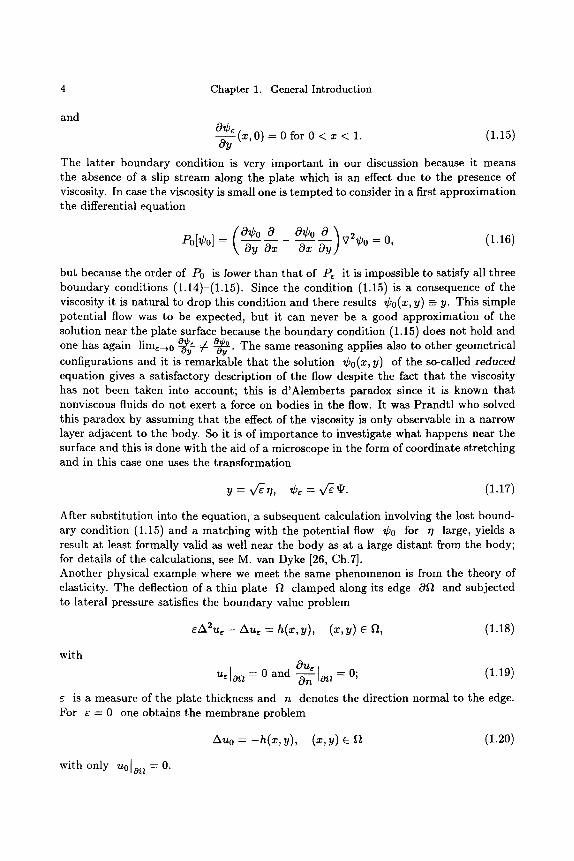
0r (x, 0) - 0 for 0 < x < 1. (1.15) Oy
The latter boundary condition is very important in our discussion because it means the absence of a slip stream along the plate which is an effect due to the presence of viscosity. In case the viscosity is small one is tempted to consider in a first approximation the differential equation
(0r 0 0r 0 ) v~r = 0, (1.16) P0[r = \ Oy Ox Ox Oy
but because the order of P0 is lower than that of Pe it is impossible to satisfy all three boundary conditions (1.14)-(1.15). Since the condition (1.15) is a consequence of the viscosity it is natural to drop this condition and there results r y) -- y. This simple potential flow was to be expected, but it can never be a good approximation of the solution near the plate surface because the boundary condition (1.15) does not hold and one has again lime-+0 ~oy =/: ~ " The same reasoning applies also to other geometrical
configurations and it is remarkable that the solution r y) of the so-called reduced equation gives a satisfactory description of the flow despite the fact that the viscosity has not been taken into account; this is d 'Alemberts paradox since it is known that nonviscous fluids do not exert a force on bodies in the flow. It was Prandt l who solved this paradox by assuming that the effect of the viscosity is only observable in a narrow layer adjacent to the body. So it is of importance to investigate what happens near the surface and this is done with the aid of a microscope in the form of coordinate stretching and in this case one uses the transformation
y = v ~ , r = v q V . (1.17)
After substi tution into the equation, a subsequent calculation involving the lost bound- ary condition (1.15) and a matching with the potential flow r for r/ large, yields a result at least formally valid as well near the body as at a large distant from the body; for details of the calculations, see M. van Dyke [26, Ch.7]. Another physical example where we meet the same phenomenon is from the theory of elasticity. The deflection of a thin plate 12 clamped along its edge 012 and subjected to lateral pressure satisfies the boundary value problem
eA2ue - Au~ = h(x,y) , (x,y) e it, (1.18)
with Oue
ue[o ~ = 0 and -~n--n [o~ - 0; (1.19)
e is a measure of the plate thickness and n denotes the direction normal to the edge. For e = 0 one obtains the membrane problem
AUo = - h ( x , y), (x, y) e fl (1.20)
with only UOlo ~ -- O.
Singular Perturbation of Boundary Layer Type
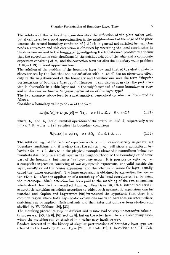
The solution of this reduced problem describes the deflection of the plate rather well, but it can never be a good approximation in the neighbourhood of the edge of the plate because the second boundary condition of (1.19) is in general not satisfiedby u0. One needs a correction and this correction is obtained by stretching the local coordinates in the direction normal to the boundary. Investigating the transformed problem it appears that the correction is only significant in the neighbourhood of the edge and a composite expression consisting of u0 and the correction term satisfies the boundary value problem (1.18)-(1.19) in good approximation. The solution of the problem of the boundary layer flow and that of the elastic plate is characterized by the fact that the perturbation with e small has an observable effect only in the neighbourhood of the boundary and therefore one uses the term "singular perturbations of boundary layer type". However, it can also happen that the perturba- tion is observable in a thin layer not in the neighbourhood of some boundary or edge and in this case we have a "singular perturbation of free layer type" The two examples above lead to a mathematical generalization which is formulated as follows. Consider a boundary value problem of the form
eL2[ue(x)]+Ll[ue(x)]=f(x), x E ~ t C ] R ~ , 0 < e < < l , (1.21)
where L2 and L1 are differential operators of the orders m and k respectively with m > k > 0, while u~(x) satisfies the boundary conditions
B~[ue(x)] = qo~(x), x E af~, g = 0 , 1 , 2 , . . . . (1.22)
The solution u0 of the reduced equation with e - 0 cannot satisfy in general all boundary conditions and it is clear that the solution ue will show a nonuniform be- haviour for E -+ 0. Just as in the phsyical examples above this nonuniform behaviour manifests itself only in a small layer in the neighbourhood of the boundary or of some part of the boundary, but also a free layer may occur. It is possible to write ue as a composite expression consisting of two asymptotic expansions, one valid outside the layer, usually called the "outer expansion" and the other valid inside the layer, usually called the "inner expansion". The inner expansion is obtained by expanding the opera- tor eL2 + L1 after the application of a stretching of the local coordinates, i.e. by using the microscope. Much attention has been paid to the matching of the two expansions which should lead to the overall solution u~. Van Dyke [26, Ch.5] introduced certain asymptotic matching principles according to which both asymptotic expansions can be matched and Kaplun and Lagerstrom [90] introduced the hypothesis that there is a common region where both asymptotic expansions are valid and that an intermediate matching can be applied. Both methods and their interrelation have been studied and clarified by W. Eckhaus [30], [33]. The matching procedure may be difficult and it may lead to very unattractive calcula- tions, see e.g. [53, Ch.6], [62, section 8], but on the other hand there are also many cases where the matching can be attained in a rather easy intuitive way. Readers interested in the history of singular perturbations of boundary layer type are referred to the books by M. van Dyke [26], J.D. Cole [19], J. Kevorkian and J.D. Cole
Chapter 1. General Introduction
[85], P.A. Lagerstrom [90], R.E. O'Malley [112], the paper by K.O. Friedrichs [45] and the SIAM-Review, Vol 36, 1994.
While applied mathematical research was aimed at asymptotic approximations of solutions and procedures were invented to construct these approximations in a more or less formal way there was also the mathematical question regarding the validity of these procedures. Early investigations in this direction were carried out by a . o . W . Wasow [139] in 1944, N. Levinson [95] in 1950, O.A. Oleinik [114] in 1954, I.M. Visik and L.A. Lyusternik [137], [138] in 1957. Meanwhile the subject has received a broad interna- tional interest stimulated from many research activities and there exists nowadays an overwhelming vast quantity of literature. We do not aim at a complete bibliographical survey and therefore we present in the list of references a number of publications com- posed according to the subjective taste and knowledge of the authors, see [100, 70, 29, 30, 111, 112, 55, 64, 9, 41,101]. Readers will certainly miss some names and important papers which should also be mentioned. However many additional references will be found in the publications quoted and in those still to be quoted in the chapters to follow where we explain a large numbers of topics of the theory of singular perturbations.
In this textbook we give our attention primarily to the construction of formal ap- proximations to solutions of initial and boundary value problems and to the validity of these formal approximations. The latter is justified by a careful investigation of re- mainder terms, being the difference between the solution and its formal approximation. This involves quite a number of mathematical techniques, such as the use of Gronwal- l's lemma, the contraction principle in Banach spaces, a priori estimates of solutions of boundary and initial value problems using the maximum principle and energy esti- mates. Although a number of physical applications are included, mostly in the context of oscillation problems, the emphasis is on mathematical analysis. Excellent texts on the applications of singular perturbation theory in many examples from mathematical physics and engineering are the books by J.D. Cole [19], J. Kevorkian and J.D. Cole [85], R.E. O'Malley [112], D.R. Smith [127] and A. Nayfeh [108].
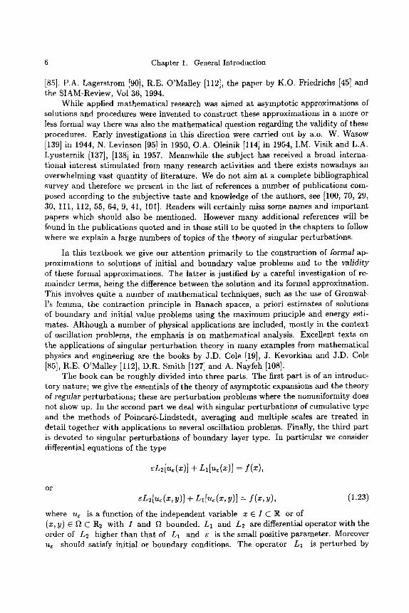
The book can be roughly divided into three parts. The first part is of an introduc- tory nature; we give the essentials of the theory of asymptotic expansions and the theory of regular perturbations; these are perturbation problems where the nonuniformity does not show up. In the second part we deal with singular perturbations of cumulative type and the methods of Poincar6-Lindstedt, averaging and multiple scales are treated in detail together with applications to several oscillation problems. Finally, the third part is devoted to singular perturbations of boundary layer type. In particular we consider differential equations of the type
r + Ll[u~(x)] = f(x),
o r
r y)] + Ll[Ue(X, y)] = f(x, y), (1.23)
where ue is a function of the independent variable x C I C R or of (x,y) E f~ C JR2 with I and 12 bounded. L1 and L2 are differential operator with the order of L2 higher than that of L1 and 6 is the small positive parameter. Moreover ue should satisfy initial or boundary conditions. The operator L1 is perturbed by
Singular Perturbation of Boundary Layer Type
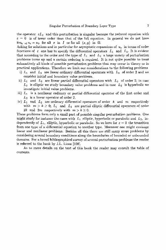
the operator eL2 and this perturbation is singular because the reduced equation with - 0 is of lower order than that of the full equation. In general we do not have
lime_~oue--uo for all x in I or for all (x,y) in ~t. Asking for solutions and in particular for asymptotic expansions of ue in terms of order functions of ~ one has to specify the differential operators L1 and L2. It is evident that according to the order and the type of L1 and L2 a large variety of perturbation problems turns up and a certain ordering is required. It is not quite possible to treat exhaustively all kinds of possible perturbation problems that may occur in theory or in practical applications. Therefore we limit our considerations to the following problems
i) L1 and L2 are linear ordinary differential operators with L2 of order 2 and we consider initial and boundary~value problems.
ii) L1 and L2 are linear partial differential operators with L2 of order 2; in case L2 is elliptic we study boundary value problems and in case L2 is hyperbolic we investigate initial value problems.
iii) L1 is a nonlinear ordinary or partial differential operator of the first order and L2 is a linear operator of order 2.
iv) L1 and L2 are ordinary differential operators of order k and m respectively with m > k :> 0; L1 and L2 are partial elliptic differential operators of order 2k and 2m respectively with m > k > 0.
These problems form only a small part of possible singular perturbation problems. One might study for instance the cases with L1 elliptic, hyperbolic or parabolic and L2, in- dependently of L1, elliptic, hyperbolic or parabolic. So we have for 6 = 0 the transition from one type of a differential equation to another type. Moreover one might envisage linear and nonlinear problems. Besides all this there are still many more problems by considering several boundary conditions along the boundaries of bounded or unbounded domains. For a broad bibliographical survey of several perturbation problems the reader is referred to the book by J.L. Lions [100].
As to more details on the text of this book the reader may consult the table of contents.

This Page Intentionally Left Blank
Chapter 2
A S Y M P T O T I C E X P A N S I O N S
1. O r d e r Symbols
In the preceding introduction we have acquainted the reader with some problems concerning the approximation of solutions of differential equations and therefore we devote our at tention first to approximations of functions in general. In case one has a sequence of numbers, say { f ( n ) } ~ = 1 , the number which may be approached by this sequence for n --4 oo is well known and is denoted by lim f (n) , in case this limit
n - - + cx)
exists. If lim f ( n ) = f , then we have the following situation: given any ~ > 0 there n - - - ~ OO
exists a number N(e), dependent on e, such tha t
If(n) - fl < e, Vn > N(e). (2.1.1)
This definition tells us something about the behaviour of f ( n ) for n --4 c~, namely that f ( n ) approaches the number f as close as we want by increasing the number n, but it does not tell _how f ( n ) approaches the number f , and the definition does not give much information about the difference between f (n) and f when n becomes very large; it follows only that this difference approaches zero. In order to describe the behaviour of sequences of numbers in a more precise way, one compares different sequences of numbers in the following way
DEFINITION 1
i) The order of { f ( n ) } ~ = 1 is for n -+ c~ not higher than tha t of {g(n)}~=l, whenever there exist numbers A and N such tha t
If(n)l < A[g(n)l, Vn > N. (2.1.2)
This is expressed by the Bachmann-Landau notat ion [92]
f ( n ) = O(g(n)) for n sufficiently large (2.1.3)
ii) The order of { f ( n ) } ~ = 1 is for n --4 cx~ lower than tha t of {g(n)}~=l , whenever there exists for any positive number r/, a number N(r/), dependent on r/, such that
If(n)] < ~]g(n)l , kin > g(r / ) . (2.1.4)
10 Chapter 2. Asymptotic Expansions
This is expressed by the Bachmann-Landau nota t ion
f (n) = o(g(n)) for n sufficiently large. (2.1.5)
iii) The order of { f (n )}~= 1 is for n -+ co equal to tha t of {g(n)}~= 1, whenever f (n) : O(g(n)) and f (n) :fi o(g(n)) for n sufficiently large. This is expressed by the nota t ion
f (n) = 08(g(n)) for n sufficiently large. (2.1.6)
R e m a r k s 1. In case g(n) is not zero for n sufficiently large, and in the par t icular circumstance
tha t the limit of I f--(-~ ] exists, the defining relations (2.1.2) and (2.1.6) may be 9(-) replaced by
f (n) (2.1.7) l i r n [ g - ~ I = ~ # 0.
The reader should be warned tha t the relation (2.1.7) is much more restrictive than (2.1.2), and so it cannot be used as a definition of the "0" symbol
2. Similar definitions hold whenever the discrete variable n is replaced by a continuous variable w with w E R and w -+ co. The same applies also when w is replaced by the variable ~ with e E R and E $ 0 (define e = 1/w).
E x a m p l e s 1. s i n ( n ) = 0 ( 1 ) for h E N and n - -+co ,
s i n w : 0 ( 1 ) for w E R and w--+co. 2. s i n ( 1 / n ) = o ( 1 ) for h E N and n - -+co ,
s i n E = o ( 1 ) for ~611( and E--+0. 3. l o g ( l + e ) : 0 8 ( e ) and l o g ( l + e ) = o ( e ~'), # < 1 for e E R and e - -+0 4. e ~ - l = 0 8 ( e ) for e - + 0 and e ~ - l = 0 8 ( e ~) for w - - + + c o 5. e -1/~ : O(e"), Vn, e E R and e $ 0.
e -1/~ is called "asymptot ical ly equal to zero for e $ 0." The definitions are easily extended to sequences of functions f (x , n) depending on a variable x and the discrete pa ramete r n or to sets of functions f (x , w) or f ( x , e) de- pending on x and the continuous paramete r w and ~ respectively.
In the following we restrict our t r ea tmen t only to the case e E R and e --+ 0, and the functions f ( x , e ) and g(x,e) to be compared with each other are defined for x - ( S ) i n a d o m a i n D C R " .
DEFINITION 2 i) The order of f (x , e) is not higher than tha t of g(x, ~) at the point x = x0 E D for
$ 0 whenever there exist positive functions k(x) and e(x) such tha t
If(x0,e)l < k(xo)[g(xo, e)l for 0 < e < e(x0). (2.1.8)
Notation: f(xo, e) = 0(g(x0, e)), ~ $ 0. If (2.1.8) holds at each point x 6 D, we write
f (x ,~) -- O(g(x,~)), x E D, ~ $ 0.
1. Order Symbols 11
ii) The order of f (x ,e) is lower than tha t of g(x,e) at the point x0 6 D for e $ 0 whenever for any positive number 7/ there exists a positive function
6n(x0) , depending on ~ and x0 such tha t
If(xo, e)[ < nlg(xo, e)l for 0 < e < 6n(xo ). (2.1.9)
Notation: f(xo, 6) = o(g(xo, e)), e $ 0, If (2.1.9) holds at each point x0 E D we write
f (x ,e) = o(g(x,e)), x e n , e $ O.
iii) The order of f (x , e) is equal to tha t of g(x, e) at the point x0 6 D whenever
f(xo,6) = O(g(xo,6)) and f(xo,6) # o(g(xo,6)), 6 ,~ O. (2.1.10)
Notation: f (x0 ,6) = Os(g(xo,6)). If (2.1.10) holds at each point x0 6 D we write
f (x ,e) = O,(g(x,e)), x e D, e $0.
In case the function k(x) has a finite upper bound in D with K = sup k(x) and the functions e(x) and en(x ) have a positive lower bound with
xED e - inf e(x) respectively e_ n -- inf 6n(x ) it is possible to make a uniform comparison - x6D x6D '
between the functions f (x , e) and g(x, e) as e $ 0, which is independent of the point x 6 D. So we come finally to the last definition of comparison:
DEFINITION 3 i) The order of f (x ,6) is not higher than tha t of g(x,e) uniformly in a domain
D C R '~ for e $ 0, whenever there exist positive numbers e and K such tha t
If(x,6)l < K ig(x,6), Vx 6 D, and 0 < 6 < e. (2.1.11)
Notation: f (x , e) = O(g(x, e)), uniformly in D, as 6 $ 0. ii) The order of f (x , e) is lower than tha t of g(x, e) uniformly in a domain
D C IR n for e $ 0 whenever there exists for any positive number ~, however
small, a positive number 6 n such tha t
If(x, 6)1 < ~lg(x, 6)1, Vx ~ D and 0 < 6 5 6 n. (2.1.12)
Notation: f (x ,e) = o(g(x,e)), uniformly in D as e $ 0. iii) The order of f (x , 6) is equal to tha t of g(x, e) uniformly in a domain D C ]R ~ for
e -+ 0 whenever
f (x , e) = O(g(x,e)) uniformly in D as e $ O,
but f (x, e) --/: o(g(x, e)) in D.
Notation: f (x ,e) = Os(g(x,e)) uniformly in D as e $ 0.
12 Chapter 2. Asymptotic Expansions
E x a m p l e s 1 1. ~ - ~ - 0 ( 1 ) as e $ 0 for each value of x in (0,1] but 1 is not 0(1) uniformly , ~-~
in (0, 1], because k(x) - 1/x has not a finite upper bound in (0, 1]. 2. log(sin ex) - 0(log 2ex ) uniformly in (0, 1] as ~ $ 0. We have
2~x 0 < - W - < s i n c x for 0 < x < l in 0 < ~ < 1, and therefore [log(sinr < [log (2~---~-~)[, Vx �9 (0,1] and 0 < e < 1. It follows tha t k(x) maybe taken identically equal to 1, K - 1 and e_ - 1 and hence log(sinex) - 0 ( log 2~, ) uniformly in (0, 1] e $ 0. One may also prove
log(sinex) = 08( log 2e__xx) uniformly in (0, 1], e .~ 0. 71"
This is left as an exercise to the reader. 3. e x p ( - x / r = o(r VN" at every point of (0, c~), but this result is not t rue
uniformly, because the condit ion (2.1.12) cannot be fulfilled in all points of the open interval (0, c~). When we take for example x = 61+~', # > 0 we have
e -x/e : e -e" > e -1 for 0 < e < 1.
2. G a u g e F u n c t i o n s and A s y m p t o t i c S e q u e n c e s
The order definitions give us a tool to compare the values of two functions which depend on the variable x and the paramete r e. By taking a special privileged set of functions we get a set of comparison functions with the values of which we may compare the values of a large class of functions f(x,r This special set is chosen as simple as possible (depending on the class of functions f(x,r and with this set we have obtained, so to say, a yard stick or measuring rod to be used to measure the values of our functions f (x, r as ~ $ 0. The elements of the special set are called gauge functions.
DEFINITION 4 A gauge function 5(~) is a function of the paramete r e with the propert ies of being positive, monotoneously decreasing or increasing for ~ $ 0 and continuously differen- tiable in a right neighbourhood (0, 60) of e - 0. Sets of frequently used gauge functions are the positive and the negative powers of ~ : g,`(c) -- c,`, n - 0, + l , . . . . Other useful sets are e.g.: e~'gn(6), ]loge[Ogr,(e) or exp(-1 /e)g ,~(e) with a, /3 �9 R and a > O. After this in t roduct ion of gauge functions we introduce some ordering in sets of gauge functions. So we are led to the following definition of ordering:
D E F I N I T I O N 5
The sequence {5,, (~)}~=0 of gauge functions is called an asymptotic sequence whenever
5,~+1(~) = o(5n(r Vn, as ~ $ 0. (2.2.1)
E x a m p l e s
{e,`}~--0, {r with p > 0, {[loge[~e"}.~176 0 with j3 e R, {8,`e-1/e}n~176 e x p ( - l / r = o(r for all values of n and hence exp ( -X/e ) is smaller than all gauge functions of the set {~n}n~176 0. Therefore we call e x p ( - 1 / r asymptotically zero and this is denoted by e x p ( - 1 / e ) ~ 0.
3. Asymptotic Series 13
3. A s y m p t o t i c Ser ies
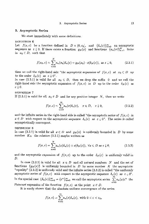
We start immediately with some definitions.
DEFINITION 6 Let f (x ,e ) be a function defined in D • (0, e0], and {6n(e)}n~__0 an asymptotic
},~=1 finite sequence as 6 $ 0. If there exists a function gg(x) and functions {a,~(x) g in x 0 E D , such that
N
f(xo, s) -- Zan(Xo)5~(~) + 9N(xO) " O(hN(~)), as e $ 0, (2.3.1) n - - O
then we call the right-hand side "the asymptotic expansion of f (x , ~) at xo E D up to the order 5N(~ ) aS e .~ 0".
In case (2.3.1) is valid for all x0 E D, then we drop the suffix 0 and we call the right-hand side the asymptotic expansion of f (x ,r in D up to the order 6N(r as e $ 0 .
DEFINITION 7
If (2.3.1) is valid for all x0 E D and for any positive integer N, then we write
o o
f (x ,e ) ,.~ Z a , ( x ) 6 , ( e ) , x E D, e $ O, (2.3.2) n----O
and the infinite series in the right-hand side is called "the asymptotic series of f (x, e) in x E D with respect to the asymptotic sequence 5~(e) as e $ 0". The series is called asymptotically convergent.
DEFINITION 8
In case (2.3.1)ia valid for all x E D and 9N(X) is uniformly bounded in D by some number KN the relation (2.3.1) maybe written as
N
f (x ,e ) = Za,~(x)6 , (r + o((~N(6)) , VX E D as ~ $ 0, (2.3.3) n - - O
and the asymptotic expansion of f (x ,r up to the order 6N(r is uniformly valid in D.
In case (2.3.1) is valid for all x E D and all natural numbers N and the set of functions {gu(x)} is uniformly bounded in D by some number K the asymptotic "equality" (2.3.2) is uniformly valid and the infinite series (2.3.2) is called "the uniformly asymptotic series of f (x, e) with respect to the asymptotic sequence 6, (e) as e $ 0".
oo
In the special case {6n (e)}oon=0 = { en }oon=0 we call the asymptotic series y] an (x)r n the n - - 0
Poincar6 expansion of the function f (x , e) at the point x E D. It is easily shown that the absolute uniform convergence of the series
(x)
f (x ,r = Zan(x )6n(r with 0 < e < Co, n - - O
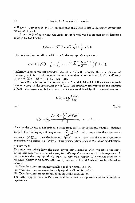
14 Chapter 2. Asymptotic Expansions
uniform with respect to x E D, implies tha t this series is also a uniformly asymptot ic series for f ( z ,e ) .
An example of an asymptot ic series not uniformly valid in its domain of definition is given by the function
f (x,6) = "~/x + 6 = v/'x �9 + - , x > O . X
This function has for all x with x > 0 the asymptot ic expansion
6 6 2 f (x , 6),~ V'~(1 + 2--x - 8x 2
. . . . + ( - 1 ) ' - l ( 2 n - 3)!! 6 n ~-,~ (;) +...),
uniformly valid in any left bounded interval x > ~ > 0; however, the expansion is not uniformly valid in x > 0 because the remainder after n terms is not 0(6~), uniformly in x > 0. ( ( 2 n - 3 ) ! ! - 1 - 3 . 5 . . . ( 2 n - 3)).
From the definition of the o-symbol and from definition 7 it follows tha t the coef- ficients an(x) of the asymptot ic series (2.3.2) are uniquely determined by the function f (x , 6); one proves simply tha t these coefficients are defined by the recurrent relations
ao(x) = l i m f (x, 6) ~,o ~o(~)
and (2.3.4)
n--1 f (x, 6) - ~ ai(x)e~i(c)
an (x) = lim i=0 ~,0 ~n(e) , n = l , 2 , . . . .
However the inverse is not t rue as is clear from the following counterexample. Suppose o o
f (x ,6) has the asymptot ic expansion, ~ an(x)6 n, with respect to the asymptot ic n = 0
sequence {6n},~~176 , then the function f (x , 6) + exp ( - 1 / 6 ) has the same asymptot ic expansion with respect to {6n}n~176 . This consideration leads to the following definition.
DEFINTION 9
Two functions which have the same asymptot ic expansion with respect to the same asymptot ic sequence are called asymptotically equal with respect to this sequence. A function is called asymptot ical ly equal to zero with respect to a certain asymptot ic sequence whenever all coefficients an(x) are zero. This definition may be applied as follows:
i) Two functions are asymptot ica l ly equal in a point x E D. ii) Two functions are asymptot ica l ly equal in all points x E D.
iii) Two functions are uniformly asymptot ical ly equal in D. The la t ter applies only in the case tha t bo th functions possess uniform asymptot ic expansions.
3. Asymptotic Series 15
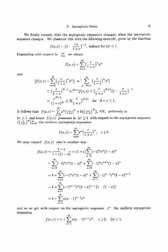
We finally remark, that the asymptotic expansion changes, when the asymptotic sequence changes . We illustrate this with the following example, given by the function
ex ) -1 defined for Ixl < 1. f ( x , r ( 1 - l + e '
r Expanding with respect to 1-~ we obtain
o o
-C ) nxn S(x,e) = E ( 1 + e
r ~ - - O
and N o o
Z ( If(~' ~) - ~ - ~ ( 1 + ~ l + e n=O n = N + l
e )N+I(1 - e )-1 )N+llxIN+lf(x 'c) <-- (1 + e 1 + e < - ( l + e
_ e g+l e ) g + l for O < e _ < l . -- (1 -it- ~) N ~ 2 ( 1 + e
N It follows that f (x, e) - y~. x ~ (y~) '~ + 0{ ( ~ ) N }, VN, uniformly in
r t = 0
Ixl <_ 1 and hence f (x , e) possesses in Ixl < 1 with respect to the asymptotic sequence n O0 { (Y g T) }~=0 the uniform asymptotic expansion
o o
1" so. f ( x , e ) , . . , x" (1 + e , r ~ = 0
We may expand f ( x , e ) also in another way:
l + e oo f ( x , e ) = 1 + e(1 - x) = (1 + r - x) n
n - - 0
o o o o
= E ( - 1 ) n e ' ~ ( 1 - x) '~ + E ( - 1 ) n e ' ~ + l ( 1 - x) '~ n=O n=O
= 1 + E ( - 1 ) ' ~ e " ( 1 - x) n + E ( - 1 ) n - l e ~ ( 1 - x) ~-1 n--'- 1 n = l
o o
= 1 + E ( - 1 ) ' ~ - l e " ( 1 - x )n- l{1 - ( 1 - x)} n - - 1
o o
= 1 + E x ( x - 1)n-ze '~ n - - - 1
and so we get with respect to the asymptotic sequence e n the uniform asymptotic expansion
f ( x , e) ~., 1 + ~ _ x ( x - 1)n--lr n, S .~ O, I~1 _< 1. n = l
16 Chapter 2. Asymptotic Expansions
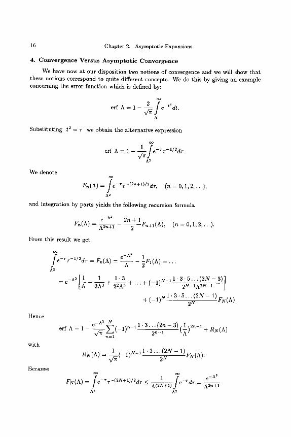
4. Convergence Versus A s y m p t o t i c Convergence
We have now at our disposition two notions of convergence and we will show that these notions correspond to quite different concepts. We do this by giving an example concerning the error function which is defined by:
o o
2 / _t ~ erf A = 1 v/~ e dt.
A
Substi tut ing t 2 - T we obtain the alternative expression
erf A = 1 - -
c ~ 1/ e-rT-1/2dT"" A2
We denote o o
F, (A) = / e - ~ T - ( 2 " + l > / 2 d . r , (n -- 0,1, 2, . . .) ,
A 2
and integration by parts yields the following recursion formula
_ A 2 e 2 n + l F , (A) - h2 ,+ 1 2 F ,+I (A) , (n = 0, 1 ,2 , . . . ) .
From this result we get
o o - A 2
e - rT-1 /2dT = F0(A) - e 1 h 2 FI(A) . . . .
A 2
-A2[ 1 1 1"3 ] ---- e A 2A 3 + 2-5~A 5 -}- -}-(_I)N_ 1 1 . 3 . 5 . . . ( 2 N - 3)
+ (_1) N 1 . 3 . 5 . . . ( 2 N - 1) ' 2N FN(A).
Hence
with
Because
erf A = 1 _ A a N
e ) , - 1 1 " 3.2~(_2 ~ - 3) 1 2,~-1 v ~ ~'-~(-1 (X) + RN(A)
n - - 1
1 1)g+ 11. 3.. . ( 2N- 1) R~(A) = - -~( - 2~ F~(A).
c ~ r - A 2 / 1 / e FN(A) - e -rT-(2N+l)/2dT" < A(2N+I ) e - ' d T = h2 ,+ 1
A 2 A 2
4. Convergence Versus Asymptotic Convergence 17
we have 1 1 . 3 . . . ( 2 N - 1) e - n 2
IRN(A)I < 2 N A2N+I '
and therefore
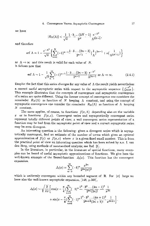
e-A2( N 2~(2_~_in 1 2n-1 1 } erf A -- 1 - ~ ~--~(-1) n-1 1 . 3 . - 3) ( ~ ) + O(A2g_ 1 ) n - - 1
as A -4 co and this result is valid for each value of N. It follows now that
1 ~ .2: (_21n erf A ~ 1 ~ . ~ _ (_1),~_ 1 1 . 3 - - 3) e -As _ A2n_ 1 as A -4 co. (2.4.1)
Despite the fact that this series diverges for any value of A the result yields nevertheless
a correct useful asymptotic series with respect to the asymptotic sequence { A2n+l ~-A2 }. This example illustrates that the concepts of convergence and asymptotic convergence of a series are quite different. Using the former concept of convergence one considers the remainder RN(A) as function of N keeping A constant, and using the concept of asymptotic convergence one consider the remainder RN(A) as function of A keeping N constant.
The same applies, of course, to functions f(x, A) depending also on the variable x or to functions f (x , r Convergent series and asymptotically convergent series represent totally different points of view; a well convergent series representation of a function may be bad from the asymptotic point of view and a correct asymptotic series may be even divergent.
An interesting question is the following: given a divergent series which is asymp- totically convergent, find an estimate of the number of terms which gives an optimal approximation of f(r or f(x, 6) where e is a given fixed small number. This is from the practical point of view an interesting question which has been solved by a .o . I , van den Berg, using methods of nonstandard analysis; see Ref. [5].
In the literature, in particular, in the literature of special functions, many exam- ples can be found of useful asymptotic approximations of functions. We give here the well-known example of the Bessel-function Jo(x). This function has the convergent expansion.
oo
= 22~(n!) 2
n - - 0
which is uniformly convergent within any bounded segment of IR. For Ix[ large we have also the well-known asymptotic expansion, [148, p.368],
2 c o s ( x - lr (_1) n l 2. 3 2 . . . ( 4 n - 1) 2 1 Jo(x) ",-' ~ n=o 26n (2n)! x2~
7r,~v,( ] ~ 1 2 . 3 2 . . . ( 4 n + 1 ) 2 1 ] + sin(x 'A--- ' ' - l ' r~ 26"+3(2n + 1)' x 2"+----~ J
D
~r~,-'- 0
18 Chapter 2. Asymptotic Expansions
While the convergent expansion is rather useless for getting values of Jo(x) for large values of x, the asymptotic series is very useful. In order to obtain an approximate value of J0(3) up to three numerals one needs eight terms of the convergent expansion and only one term of the asymptotic expansion.
5. Elementary Operations on Asymptotic Expansions
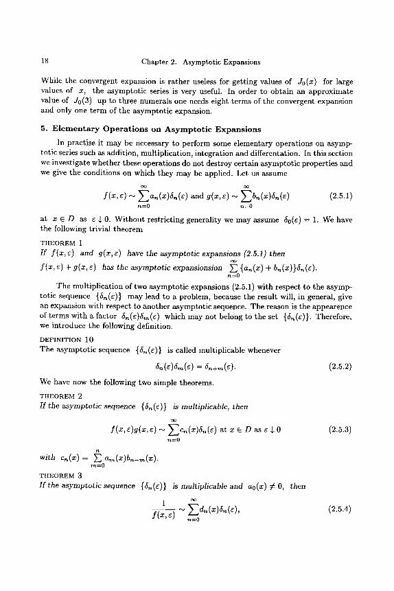
In practise it may be necessary to perform some elementary operations on asymp- totic series such as addition, multiplication, integration and differentation. In this section we investigate whether these operations do not destroy certain asymptotic properties and we give the conditions on which they may be applied. Let us assume
f (x , e ) ,,~ Ea,(X)hn(r and g(x, r ,',., Ebn(x)5 , (6) (2.5.1) n = 0 n = 0
at x C D as c $ 0. Without restricting generality we may assume 60(e) = 1. We have the following trivial theorem
THEOREM 1 If f (x,e) and g(x,e) have the asymptotic expansions (2.5.1) then
oo
f (x ,e) + g(x,e) has the asymptotic expansionsion E {an(x) + bn(x)}5,(e). n - - O
The multiplication of two asymptotic expansions (2.5.1) with respect to the asymp- totic sequence {fin(e)} may lead to a problem, because the result will, in general, give an expansion with respect to another asymptotic sequence. The reason is the appearence of terms with a factor 5n(r which may not belong to the set {6n(r Therefore, we introduce the following definition.
DEFINITION 10 The asymptotic sequence {6,,(~)} is called multiplicable whenever
5. (6)6m (r = 5n+.~ (e). (2.5.2)
We have now the following two simple theorems.
THEOREM 2 If the asymptotic sequence {hn(~)} is multiplicable, then
oo
f(x,e)g(x,r ~ Ecn(x)6~(r at x E D as r $ 0 (2.5.3) n - - 0
n
with Cn (x) = ~ am (x)bn_m(x). m - - O
THEOREM 3 If the asymptotic sequence {6n(r is multiplicable and ao(x) ~ O, then
1 o~ f(x, 6) "" Ed"(x)6"(r (2.5.4)
r~"-O
5. Elementary Operations on Asymptotic Expansions 19
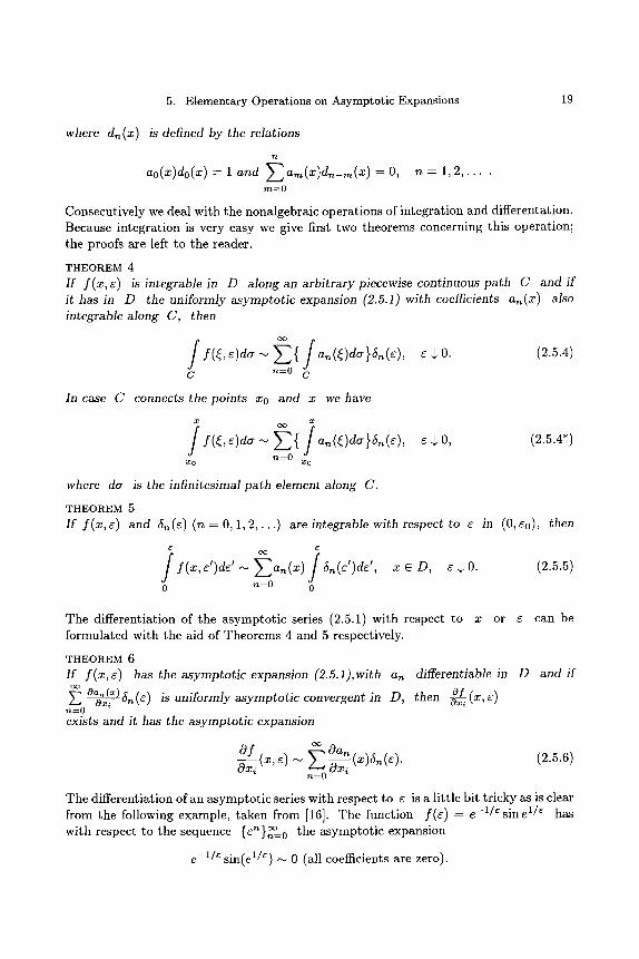
where dn(x) is defined by the relations
n
ao(x)do(x) = 1 and E a m ( x ) d n _ m ( X ) = O, n - 1,2, . . . . m"-O
Consecutively we deal with the nonalgebraic operat ions of integrat ion and differentation. Because integrat ion is very easy we give first two theorems concerning this operation; the proofs are left to the reader.
T H E O R E M 4 If f (x, ~) is integrable in D along an arbitrary piecewise continuous path C and if it has in D the uniformly asymptotic expansion (2.5.1) with coemcients an(x) also integrable along C, then
oo
C n = 0 5
In case C connects the points xo and x we have
/ / f(~,~)d~ ~ ~ { a~(~)d~}~(~), ~ S O, (2.5.4*) n--O
xO Xo
where do" is the infinitesimal path element along C.
T H E O R E M 5
0 n = 0 0
The differentiation of the asymptot ic series (2.5.1) with respect to x or c can be formulated with the aid of Theorems 4 and 5 respectively.
T H E O R E M 6 If f (x ,e) has the asymptotic expansion (2.5.1),with an differentiable in D and if
oo Oa X) O f Y~ ~( an(e) is uniformly asymptotic convergent in D, then -8-~, (x, e)
n--O
exists and it has the asymptotic expansion
Of oo Oan (x)Sn(c ) (2.5.6) ~ �9
n--O
The differentiation of an asymptot ic series with respect to e is a little bit tricky as is clear from the following example, taken from [16]. The function f ( s ) = e -1/~ s ine 1/~ has with respect to the sequence {en}~=0 the asymptot ic expansion
e -1/~ sin(e 1/~) ,,~ 0 (all coefficients are zero).
20 Chapter 2. Asymptotic Expansions
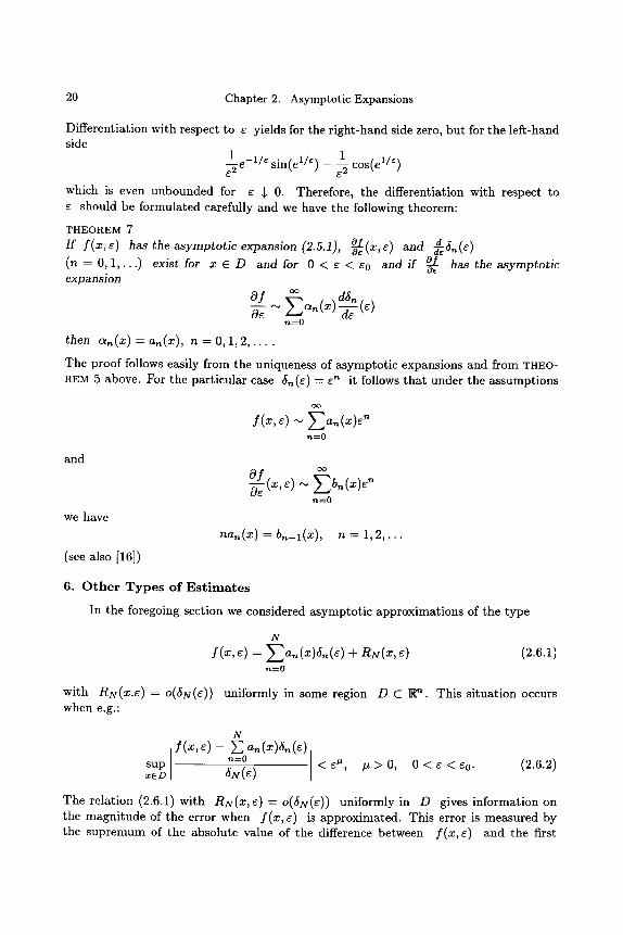
Differentiation with respect to e yields for the right-hand side zero, but for the left-hand side
1 cos(el/~ ) 1 -1/~ sin(el/~) ~-2 e-~e
which is even unbounded for e ~ O. Therefore, the differentiation with respect to e should be formulated carefully and we have the following theorem:
T H E O R E M 7
I f f ( x , e ) has the asymptotic expansion (2.5.1), of( and d6n(e )
(n -- 0,1, .) exist for x E D and for 0 < e < eo and if of has the asymptotic "" Og
expansion Of oo d6,`
n - - 0
then a , ( x ) = an(x), n - O , 1 , 2 , . . . .
The proof follows easily from the uniqueness of asymptotic expansions and from T H E O -
REM 5 above. For the particular case 6,, (s) - ~,` it follows that under the assumptions
and
we have
(see also [16])
(x)
f (x ,e) , ,~ ~-~a,`(x)c n
O f oo
, ` - - 0
na,`(x) = b , - l (X) , n = 1 ,2 , . . .
6. Other T y p e s of E s t i m a t e s
In the foregoing section we considered asymptotic approximations of the type
N
f (x , r = ~-~an(x)6n(r RN(X,r (2.6.1) n - - 0
with RN(X.r = O(6N(r uniformly in some region D C R,`. This situation occurs when e.g.:
sup x E D
N
f (x, ~) -- ~ an (x)6n (~) n - - 0
6N(~) < e u, # > 0 , 0 < e < e 0 . (2.6.2)
The relation (2.6.1) with R g ( x , e ) = o(6g(e)) uniformly in D gives information on the magnitude of the error when f ( x , e) is approximated. This error is measured by the supremum of the absolute value of the difference between f ( x , e ) and the first
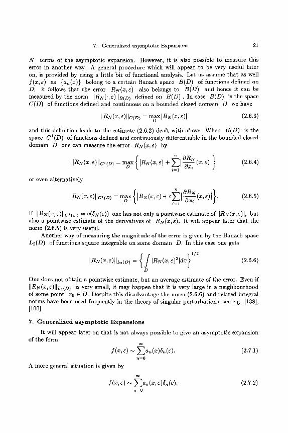
7. Generalized asymptotic Expansions 21
N terms of the asymptot ic expansion. However, it is also possible to measure this error in another way. A general procedure which will appear to be very useful later on, is provided by using a little bit of functional analysis. Let us assume tha t as well f(x,~) as {a,~(x)} belong to a certain Banach space B(D) of functions defined on D; it follows tha t the error RN(X,r also belongs to B(D) and hence it can be measured by the norm [IRN(',e)IIB(D) defined on B(D). In case B(D) is the space C(D) of functions defined and continuous on a bounded closed domain D we have
IIR~(~, ~)llc(m - m~x IR~(~, ~)1 (2.~.3)
and this definition leads to the es t imate (2.6.2) dealt with above. When B(D) is the space CI(D) of functions defined and continuously differentiable in the bounded closed domain D one can measure the error Ry(x, c) by
IIR~(~,~)II~(,) - ~ x IR~(~,~)+ I - b ~ (~,~)1 (2.6.4) i - -1
or even al ternat ively
{ } IIRN(~,~)IIC~(D) = m~x IRN(~,~) + . ( 2 . 6 . 5 )
i = 1
If ]lRg(x, e)llcl(D ) -- o(bg(~)) one has not only a pointwise es t imate of DRy(x, e)l , but also a pointwise es t imate of the derivatives of Ry(x, ~): It will appear later tha t the norm (2.6.5) is very useful.
Another way of measuring the magni tude of the error is given by the Banach space L2(D) of functions square integrable on some domain D. In this case one gets
{/ IIRN(x,e)IIL2(D) = IRg(x,e)2ldx (2.6.6)
D
One does not obtain a pointwise est imate, but an average es t imate of the error. Even if IIRy(x,e)llL2(D) is very small, it may happen tha t it is very large in a ne ighbourhood of some point x0 E D. Despite this disadvantage the norm (2.6.6) and related integral norms have been used frequently in the theory of singular per turbat ions; see e.g. [138], [100].
7. Generalized asymptotic Expansions
It will appear later on tha t is not always possible to give an asymptot ic expansion of the form
S(x,c) ~ Ea,~(x)bn(~). (2.7.1) n = 0
A more general s i tuat ion is given by
oo
f(x,~) ~ Ean(x,~)bn(e). (2.7.2) n = 0
22 Chapter 2. Asymptotic Expansions
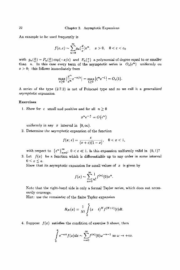
An example to be used frequently is
(x)
n - - - 0
x > 0 , 0 < 6 < 6 0
with gn (-~) = P,-, (~) exp(-x /6) and P . (~) a polynomial of degree equal to or smaller than n. In this case every term of the asymptotic series is 08(6 n) uniformly on x > O; this follows immediately from
x n e_Z/s max [ ~ - I = m~x I , ' " ~ - ~ 1 - - 0 8 ( 1 ) . =>0 ~_>0
A series of the type (2.7.2) is not of Poincar6 type and so we call it a generalized asymptotic expansion.
Exerc i se s
1. Show for 6 small and positive and for all n _ 0
x"e -~- = 0 ( 6 " )
uniformly in any x interval in [0, c~).
2. Determine the asymptotic expansion of the function
G
f(x; 6) = (x + 6)(1-- x) ' 0 < x < 1,
with respect to {6"}n~176 0 < 6 << 1. Is this expansion uniformly valid in (0, 1)?
3. Let f (x) be a function which is differentiable up to any order in some interval O < x < a . Show that its asymptotic expansion for small values of x is given by
o o
f (x) ~ ~-" l f(") (O)xn. z...~n!" n--O
Note that the right-hand side is only a formal Taylor series, which does not neces- sarily converge. Hint: use the remainder of the finite Taylor expansion
x
1 / ( x - t )gf(g+l)(t)dt . n ~ ( ~ ) =
0
4. Suppose f (x) satisfies the condition of exercise 3 above, then
o o
f e -"Xf(x)dx ~ ~-'~f(n)(O)w -~-1 as w -+ +oo. 0 n - - O
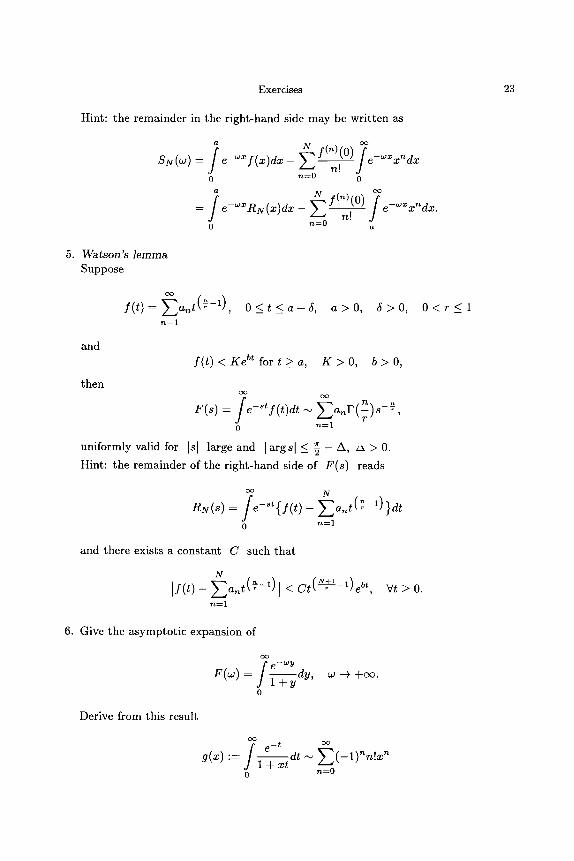
Exercises 23
Hint: the remainder in the right-hand side may be written as
SN(W) - e_.,~ f ( x )d x _ ~ f(")(O)n! e-~*x"dx 0 n = 0 0
N/(-) (0) -- e - ~ R N ( x ) d x - e - ~ x ~ d x .
n! 0 n = O a
5. Watson 's lemma Suppose
o o
f ( t ) - - E a n t ( ~ - l ) n = l
, 0 _ ~ t _ ~ a + 5 , a > 0 , 5 > 0 , 0 < r < l
and
then
f ( t ) < K e bt f o r t _ > a , K > 0 , b > 0 ,
o 0 o o
F(s) - / e - ~ t f ( t ) d t ~ ~-~a"r(n-)s-e'r 0 n = l
uniformly valid for Is[ large and [arg s[ _< 2 - A, ~ > O.
Hint" the remainder of the right-hand side of F(s) reads
cx~ N
RN(S) = / e - ~ t { f ( t ) - E a ~ t ( ~ - l ) } d t 0 n = l
and there exists a constant C such that
N I f ( t ) - E a n t ( ~ - l ) J ~_ Ct (N+~-l)ebt,
n = l
V t > 0 .
6. Give the asymptotic expansion of
o o
/ e-wy dy, F(w) = 1 + y o
w --+ +cr
Derive from this result
o o
g(~) .= f ~-~ l + x t 0
dt ~ E ( - 1 ) ' ~ n ! x n n ~ 0
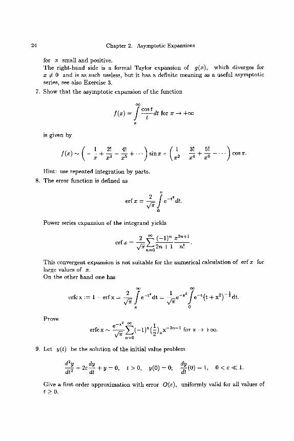
24 Chapter 2. Asymptotic Expansions
for x small and positive. The right-hand side is a formal Taylor expansion of g(x), which diverges for x r 0 and is as such useless, but it has a definite meaning as a useful asymptotic series, see also Exercise 3.
7. Show that the asymptotic expansion of the function
o o
f (x) = f costt
~g
dt for x -4 +cx~
is given by
f (x) ~ ( -~ ~ . . . s i n x + ~ - ~ - x 4 + x 6 cosx. x x 3 x 5
Hint" use repeated integration by parts.
8. The error function is defined as
x 2 / erf x -- - ~ e -t2 dt.
o
Power series expansion of the integrand yields
2 ~ ( - 1 ) " x 2"+1 err X
2n + 1 n! n - - O
This convergent expansion is not suitable for the numerical calculation of erf x for large values of x. On the other hand one has
(x) o o
2 / 1 x2 1 e r f c x : - - l - e r f x = ~ e - t : d t - ~ e - e - t ( t + ) - ~ d t .
x 0
Prove e v - - - , , , - x 2 o~ 1 - - 2 n - - I
erfcx ~ ~ / ~ j ( - - 1 ) n ( ~ ) n x for x --+ +cx). v n - -O
9. Let y(t) be the solution of the initial value problem
~t dy d2---~Y+2e + y = O , t > O , y(O)=O; - ~ - ( 0 ) = 1 , 0 < ~ < < 1 dt 2
Give a first order approximation with error O(E), uniformly valid for all values of t > 0 .
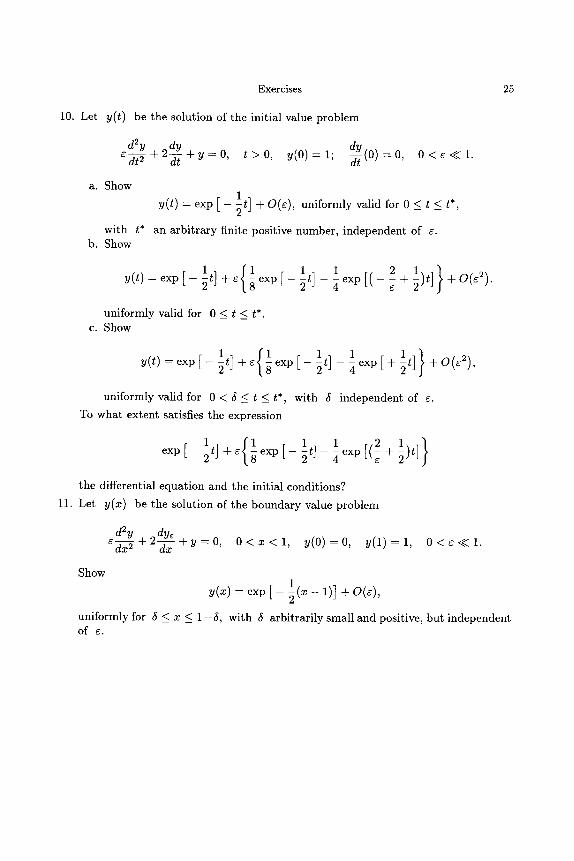
Exercises 25
10. Let y(t) be the solution of the initial value problem
d2y dy dy e-d--t-ff+2-d-~+y=O , t>O, y(O)=l ; -~-(0)=0, O < e < < l .
a. Show
y(t) - e x p [ - 2 t] + O(e), uniformly valid for 0 _< t _< t*,
with t* an arbitrary finite positive number, independent of e. b. Show
{1 1 1 2 1 } I t ] + e e x p [ - t ] - e x p [ ( - - + )t] +O(e2). y(t) = e x p [ - ~ g 2 4 e
uniformly valid for 0 _ t _ t*. c. Show
1 1 1 } y(t) = exp [ - - ~t] + c gexp[- - ~t] -- ~ e x p [ + ~ t ] +0@2),
uniformly valid for 0 < 5 _< t _< t*, with 5 independent of e. To what extent satisfies the expression
1 1 1 2 1 } I t ] + e e x p [ - t ] - e x p [ ( - + )t] e x p [ - ~ g ~ ~ ~
the differential equation and the initial conditions? 11. Let y(x) be the solution of the boundary value problem
d2y e~-x-sx2 + 2 + y = 0 , O < x < l , y(O)=O, y(1)=1, O < e < < l .
Show 1
(x - 1)] + O(e), y(x) = e x p [ -
uniformly for 5 _< x _< 1-5, with 5 arbitrarily small and positive, but independent of e.

This Page Intentionally Left Blank
Chapter 3
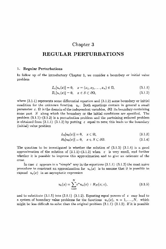
R E G U L A R P E R T U R B A T I O N S
1. Regular Perturbat ions
In follow up of the introductory Chapter 1, we consider a boundary or initial value problem
L~[u~(x)] - O, x = ( X l , X 2 , . . . , x ~ ) e gt, (3.1.1)
Be[u~(x)] = O, x e S C OFt, (3.1.2)
where (3.1.1) represents some differential equation and (3.1.2) some boundary or initial condition for the unknown function ue. Both equations contain in general a small parameter e. Ft is the domain of the independent variables, OFt its boundary containing some part S along which the boundary or the initial conditions are specified. The problem (3.1.1)-(3.1.2) is a perturbation problem and the pertaining reduced problem is obtained from (3.1.1)-(3.1.2) by putting 6 equal to zero; this leads to the boundary (initial) value problem
L o [ u o ( x ) ] = O, x e Ft, (3.1.3) B0[u0(~)] = 0, �9 e S C 03. (3.1.4)
The question to be investigated is whether the solution of (3.1.3)-(3.1.4) is a good approximation of the solution of (3.1.1)-(3.1.2) when 6 is very small, and further whether it is possible to improve this approximation and to give an estimate of the error.
In case 6 appears in a "simple" way in the equations (3.1.1)-(3.1.2) the most naive procedure to construct an approximation for u~(x) is to assume that it is possible to expand u e ( x ) in an asymptotic expression
N
u~(~) - Z ~ " , , ( ~ ) + R~(~; ~), (3.1.5) rt--0
and to substitute (3.1.5) into (3.1.1)-(3.1.2). Equating equal powers of 6 may lead to a system of boundary value problems for the fuuctions u n ( x ) , n - 1 , . . . , N , which might be less difficult to solve than the original problem (3.1.1)-(3.1.2). If it is possible
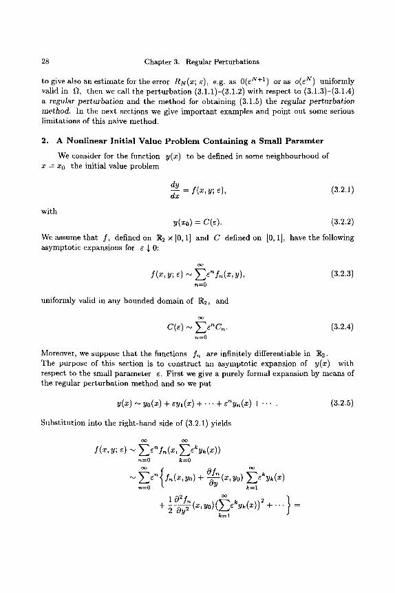
28 Chapter 3. Regular Perturbations
to give also an estimate for the error RN(X; ~), e.g. as 0(~ N+I) or as o(r N) uniformly valid in f~, then we call the per turbat ion (3.1.1)-(3.1.2) with respect to (3.1.3)-(3.1.4) a regular perturbation and the method for obtaining (3.1.5) the regular perturbation method. In the next sections we give important examples and point out some serious limitations of this naive method.
2. A N o n l i n e a r Ini t ia l Va lue P r o b l e m C o n t a i n i n g a Smal l P a r a m t e r
We consider for the function y(x) to be defined in some neighbourhood of x = x0 the initial value problem
dy d---x = f(x, y;---c), (3.2.1)
with v(~0) = c ( ~ ) . (3.2.2)
We assume that f , defined on ]I{2 • [0, 1] and C defined on [0, 1], have the following asymptotic expansions for ~ $ O:
oo
f(x,y; ~) ,,~ ~en f , , ( x , y ) , (3.2.3) t t=O
uniformly valid in any bounded domain of R2, and
oo
C(:) ~ ~-~enC,,. (3.2.4) n--O
Moreover, we suppose that the functions f~ are infinitely differentiable in R2. The purpose of this section is to construct an asymptotic expansion of y(x) with respect to the small parameter ~. First we give a purely formal expansion by means of the regular per turbat ion method and so we put
v(~) ~ v0(~) + ~u, (~) + - . . + ~ " v , ( ~ ) + . . . �9 (3.2.5)
Substitution into the right-hand side of (3.2.1) yields
o c oo
s(~, y; :) ~ ~ " s . ( ~ , Z~y~(~)) n = O k = O
~Z:" :-(~, ~0) + -~v n - - O k - - 1
1 02fn oo + . . . } _~ + ~--~y~ (~, vo) ( ~ ~ w (~)) ~
k - - 1
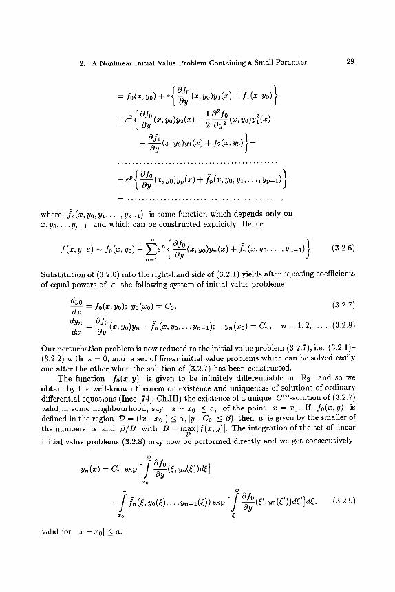
2. A Nonlinear Initial Value Problem Containing a Small Paramter 29
Ofo (~ yO)yl(~) + ]
: :0(~, v0) + ~ ~ , fl (~, y0)
1 02fo + ~ o f 0 (~, y0)y~(~) + (~, y0)y~(~)
Of 1 } -~- -~-y (X, YO)Yl(X) -t- f2(x, YO) -Jr-
} -O~y (~, yo)y,(~) + f~(~, yo, y l , . . . , y~-l)
. . . . . . . . . . . . . . . . . . . . . . . . . . . . . . . . . . . . . . . . .
where fp(x, Yo, Yl, . . . , yp-1) is some function which depends only on x, Yo,... Yp-1 and which can be constructed explicitly. Hence
c~ {OfO(x yo)Yn(X) ..~_]n(X, yO,... Yn_1) } f (~, y; ~) ~ fo(~, yo) + ~ n W ' n = l
(3.2.6)
Substitution of (3.2.6) into the right-hand side of (3.2.1) yields after equating coefficients of equal powers of e the following system of initial value problems
dyo = f0(~, y0); yo(~0) = c0, (3.2.7) dx
dy,~ Ofo = ~ ( X , yo)yn+fn(X, yO,...Yn-1); yn(Xo) =C,~, n - - 1 , 2 , . . . . (3.2.8) dx Oy
Our perturbat ion problem is now reduced to the initial value problem (3.2.7), i.e. (3.2.1)- (3.2.2) with e = 0, and a set of linear initial value problems which can be solved easily one after the other when the solution of (3.2.7) has been constructed.
The function fo(x,y) is given to be infinitely differentiable in R2 and so we obtain by the well-known theorem on existence and uniqueness of solutions of ordinary differential equations (Ince [74], Ch.III) the existence of a unique C~-solut ion of (3.2.7) valid,in some neighbourhood, say I x - x01 _ a, of the point x - xo. If fo(x,y) is defined in the region 7:) - (Ix-xol) <_ o~, ly-Col </5) then a is given by the smaller of the numbers c~ and fl/B with B - m a x l f ( x , y ) l . The integration of the set of linear
initial value problems (3.2.8) may now be performed directly and we get consecutively
x fO o yn(x) -- Cn exp[ -~y (~, yo(~))d~] Xo
~- ~ ( ~ , Y o ( ~ ) , . . . Y n - l ( ~ ) ) e x p [ -0-~y (~',yo(~'))e~']e~, x o (
(3.2.9)
valid for I x - x 0 1 _ a .
30 Chapter 3. Regular Perturbations
In this way we have obtained a formal expansion of the unknown function y(x):
oo
~ ( 3 . 2 . 5 )
n - - 0
however, we have still to prove that this formal expansion is asymptotically correct. Therefore we put
N
y(z) -- Eenyn(x) + RN(X; e), (3.2.10) n--O
and we should show that RN(X; c) = o ( E N + I ) , uniformly in I x - x01 < a. Therefore our next task is to establish the existence of Rg(x; ~) for e sufficiently small in Ix - xol < a, which yields also the existence of y(x) in I x - x0] < a for
sufficiently small, and consecutively we have to estimate the value of RN(X; e) in this interval. This is done with the aid of Liouville's method of successive approximations.
Substitution of (3.2.10)into (3.2.1)-(3.2.2) and using (3.2.7)-(3.2.8) we get for RN(x; e) the differential equation
N N dyn dx n=0 n=0
N N
= f(x, Ecnyn + RN; c ) - f(x, E e n y n ; e ) + ~N(X; e), (3.2.11) n=0 n=0
with
N N dyn
n=0 n=0 N
= f(x, Ecny,~; ~) - fo(x, yo) n----O
- - E ~ n {OfO(x 'yO)yn-t-]n(x'yO' . . . . Y n - i ) } (3 .2 .12)
n = l
The initial condition for RN(X; e) reads
N RN(XO; e) = C(e) - EenCn -- O ( e N + I ) = e N + l / z ( e ) (3 .2 .13)
n - - 0
with u(e) some bounded function of e. First, we estimate qOy(x; e). In the same way as we have obtained the asymptotic
N expansion (3.2.6) for f(x, y; e) we get for f(x, Y~ enY,~; e) an expansion which has
n - - 0
the same first (N + 1) terms and therefore
qON(X; e) = o(eN+l), uniformly in I x - x01 _< a (3.2.14)
2. A Nonlinear Initial Value Problem Containing a Small Paramter 31
The differential equation (3.2.11) with the initial condition (3.2.13) is recast into the equivalent integral equation
RN(X; E) = EN+I /2 (~) Jr- (flN(~; ~) + f(~, E E n y n ( ~ ) + RN(~; C); E)
xo n - 0
N
- s(~, ~~y~(~); ~)}e~, n--O
(3.2.15)
valid for I x - x01 < a. Successive approximation of RN(X; r gives
R ( ~ ) ( x ; c) -- g 'Nl-1/](c)
R(m-t-1)(x; ~) __ ~N-I-1//(g.)
+ ~N(~; ~) + f(~, } ~ " v . ( ~ ) + (~; ~); Xo n=0
N
- f(~,Ee'~y,~(~);--c)}d~, m = 0 , 1 , 2 , . . . (3.2.16) rt--O
Due to the smoothness of the functions { f j (x ,y ) } we have, due to (3.2.3), for each integer M
M
f(~, y:; ~) - f(~, y~; ~)1 _< ~-~'~lI~(~, y:) - f~(~, y,)l + o(~ M+~) n--O
~_ LMlY2 -- Yll + O(g'M-I-1), uniformly in any bounded domain of R2, (3.2.17)
where LM is a suitable Lipschitz-constant independent of c. Hence it follows from (3.2.16) that R(N m) - o (~g + l ) , uniformly in Ix - -xo l <_ a implies R(N m+l) --
o(~N+l) , uniformly in IX--Xol <_ a; induction on m yields that R(N m) - -O(~ g+ l ) uni- formly in I x - x01 _< a for each value of m. Further we have
N IR~>(x; ~) - R(~>(x; 6)l <_ I~ON(~;rl) + f(~, Ec'~y,~(~) + ~N+I~'(C);~)
Xo n--O N
- Ida , n--O
and so by (3.2.17) with M -- N + 1.
32 Chapter 3. Regular Perturbations
In~)(x; e) - R(~)(x; e)l -< BeN+l, uniformly for I x -- x0[ _< a, with B a suitable constant independent of e, which we take larger than 1. Further we obtain for I x - x0[ < a
n = 0 x o
" ] r t - - 0
Using (3.2.17) again we get similarly
IR(~)( ~; ~)- R(~)(~; ~)l-< nN+~ sup IR(~)(~; 6)- R(~)(~; ~)II~- ~ol Ix-xol<a
+ I~- ~01o(~ ~+~) < (L~+,B + O(~))I~- ~01~ ~§ <_ M B I x - x0le g+l , with M - LN+I + 1.
Repeating this progress again we get
1 I~ - ~01 ~ + ~ IR(N3)(x; e ) - R(~)(x; e)l _< M2B -~
and in general
R(m+l)(x; e) R y ) ( x ; e)[ < M m B l [ x xo['r'e g+l m 0,1,2, N - - - - . - - ~ ~ - (3.2.18)
uniformly valid for [x - Xo[ < a, and for e sufficiently small say 0 < e < co, e0 is independent of m. The sequence [R ( r e + l ) - R(Nm)[ is majorized by the uniformly
1 imBeN+1 convergent sequence {Mm~.lx-xo } and so we get the result that the sequence
{m } j = l
converges uniformly in Ix - x0[ < a and we obtain
1Lrno, ' IR(N"')(x; e)l < ceN+le Ma,
where C is a suitable constant, indepedent of c. It follows that the integral equation (3.2.15), and therefore also the initial value problem (3.2.11)-(3.2.13) has a solution, namely
nn(x; e ) - lim n(m)(x; e ) - o ( eg+ l ) , m - - + c x )
(3.2.19)
2. A Nonlinear Initial Value Problem Containing a Small Paramter 33
uniformly in [ x - x0[ < a. Using once again the "Lipschitz-property" (3.2.17), it can be shown that , apar t from an expression that is asymptotical ly zero, RN is the only solution satisfying (3.2.11)- (3.2.13). The final result is tha t the initial value problem (3.2.1)-(3.2.2) has a unique ssolution y(x) for [ x - x0[ < a with the property tha t we have for all values of N
o r
N N
y(~) = ~ ~ y ~ ( ~ ) + R~(~; ~) ~ ~ ~ y ~ ( ~ ) + o(~ ~§ (3.2.20) n = 0 n = 0
oo
y(x) ~ ~-'~r uniformly in I x - xo[ _< a. n - - 0
This result is s tated in the following theorem
THEOREM 1 I f the initial value problem
dyo dx = fo(x, yo), yo(~o) -Co
with fo c C ~ (R2) has its unique solution defined in the bounded segment [x - xo[ ~_ a, then the initial value problem (3.2.1)-(3.2.4)
dy oo d-~ : f ( x , y ; ~ ) ~ ~ f ~ ( x , y ) ~
n - - 0
oo
y(~0) : c (~)~ ~ c ~ ~, n - - 0
with {fn} C C ~ ( R 2 ) has also a unique solution for [ x - x o [ ~_ a. This solution possesses in I x - xo[ ~_ a the uniform asymptotic expansion
N
y(x) ~ ~-~y,~(x)r n + 0(r N = 0, 1, 2 , . . . , (3.2.20) n'- 'O
where the coefficients yn (x) (n = 1, 2 , . . . ) are determined by the recursiye set of linear initial =lue V~oblem~ (3.2. Z) ~,d (3.ZS).
R e m a r k s 1. If we make instead of the assumption (3.2.3)
oo
f(~, y; ~) ~ ~ - f ~ ( ~ , y), n ~ 0
uniformly in any bounded domain of JR2, the hypothesis
oo
cO'f (x, y; e) ,',., y ~ e ~ g,.,(x, y) (3.2.21) Oy
n'--O
34 Chapter 3. Regular Perturbations
uniformly in any bounded domain of R2 with {gn} C C~ then the assump- tion (3.2.3) holds again (see Theorem 4 of Ch.2). However, in this case the estimate (3.2.20) may be differentiated term by term with respect to x. This follows immedi- ately from the differential equation (3.2.11) and the use of the mean value theorem, which yields tha t also ddn-~ (x; ~) = 0(6N+1), uniformly in I x - x0[ < a. Hence we have besides the expansion (3.2.20) also
N ~-~Y _ ~dY"" +-gz~R~ (~; ~)~ ~ d y . . ~ + O ( ~ § n=0 n=0
(3.2.22)
uniformly in Ix - x0[ < a.
2. In case the functions fn(x, y) do not belong to C~176 but are only differ- entiable a finite number of times the asymptotic approximation (3.2.20) should be terminated after a finite number of terms. This leads to the following corollary.
COROLLARY 2 I f the initial value problem
dyo = f0(~, y0), y0(~0) = c0
dx
with fo E C1(R2) has its unique solution defined in the bounded segment I x - xo[ <_ a then the initial value problem
dy = f0(~, y) + ~f~ (~, y), u(~0) - c0 + o(~),
dx
with f l E C1(]~2) has also a unique solution in I x - xo[ (_ a and
[y(x) - yo(x)l = 0(~), un i formly in I x - xol <_ a.
The proof is left as an exercise for the reader.
3. The theorem may be generalized to the case where y(x) and f ( x , y; 6) are vector valued. The formal construction of the asymptotic expansion and the proof of its asymptotic correctness run along the same lines as above.
4. The theorem is not valid for [ x - x0[ unbounded. This follows from the fact that
the iteration procedure is no longer useful. The estimates [R ('~+1) - R(m)[ , see (3.2.18), are in unbounded intervals no longer uniformly o(eg+l) .
The corollary above to be derived from the general Theorem 1 may also be proved directly. We give this proof for the case that y(x) and f ( x , y; ~) are n-vectors. First we derive a well-known lemma, namely Gronwall's/emma.
2. A Nonlinear Initial Value Problem Containing a Small Paramter 35
LEMMA 3 Let ~ and r be nonnegative continuous functions defined for xo <__ x <_ xo + a and satisfy the relation
x
qo(x) _< 51 [ r + 52, (3.2.23)
Xo
with 51 and 52 positive constants. Then the function qo(x) satisfies the estimate
~(x) < 52 exp[51 f r162162 xo _~ x _< xo + a. (3.2.24)
XO
P r o o f It follows from (3.2.23) that
~(~) x
51 f r162 + 52 ~o
and therefore
o r
_ 1, xo < x _ x o + a ,
/ ] 5 1 ~ ) ( ~ ) ( P ( ~ ) d~ < 51 r
~o 51 f r + 52 xo Xo x /
log[51 / r + 52] - log 52 < 51 r
Xo Xo
Exponentiating both sides we get
] ] 51 ~b(~)qo(~)d~ + 52 < 52 exp[51 ~b(~)d~]
x0 x0
and using finally (3.2.23) we obtain the result (3.2.24). V]
We consider now the following perturbation problem
dy = f (~ , y) + ~g(~, y; ~), y(~o) = yo (3.2.25)
dx
with y, f and g vector valued and f continuously differentiable in Ix0, c~) • ][r and g continuous in [x0, (x)) • ]R~ • [0, 60]; further as well f as g are Lipschitz-continuous in y with Lipschitz-constants independent of x and r
THEOREM 4 Let y(x) be the solution of the initial value problem (3.2.25) with f and g satisfying the conditions stated above.
36 Chapter 3. Regular Perturbations
Moreover, let z(x) with xo <_ x <_ xo + a be the solution of the reduced initial value problem
dz -- f ( x , z), z(xo) -- Yo, (3.2.26)
dx then there exists a positive constant xl with xo < xl < xo + a such that
l y ( x ) - z(x)l = O(e), u n i f o r m l y in xo < x < xl (3.2.27)
n
(lyl 2 - ~ y ~ , etc.). i - - 1
P r o o f Let us choose an arbitrary compact and convex set 79 in [x0, cr x ]I~ with (x0, Y0) in its interior. According to the existence theorem for solutions of ordinary differential equations there exists a segment [x0, xl(e)] such that y(x) satisfies (3.2.25) for x0 < x _ xl (e) with y(x) E l) and such that z(x) satisfies (3.2.26) for x0 < x < x0 + a with z(x) E 1). Because of the continuity of g(x, y, e) in 1) x [0, e0] there can be chosen a number Xl independent of e such that y(x) satisfies (3.2.25) for x0 < x < xl , see [74], Chapter III, 3.1 and 3.3. We put y(x) = z ( x ) + w(x), and we take xl such that x0 < x < Xl < x0 + a. The function w satisfies the initial value problem
dw dx = { f (x , z(x) + w(x)) - f (x , z(x))} + ~g(x, z(x) + w(x); ~)
of = Oz (x, z(x) + O(x). w(x ) )w(x ) + eg(x, z(x) + w(x); e), (3.2.28)
where o/ is the n x n-matr ix with entries o_/x 0 < Oj(x) < 1 and the initial condition Oz Ozj '
is W(Xo) = O. Because we have taken 1) as convex, the argument (x, z(x) + O(x). w(x)) also belongs to 1) since y(x) and z(x) belong to 1). Due to f E C1(1)) we have that
Of " ~ Ofi (x, z-+-0.w)[ z + ~ w)ll j l
i----1 "-
is bounded by a positive constant C 1 , and due to g E C(1) x [0, ~0]) we have also
Ig(~, z + ~; ~)1 < c~
with C2 another positive constant, independent of ~. Integrating the differential equation (3.2.28) we get with the aid of Cauchy's inequality
Of (~, z(~) -+- 0(~). w(~))w(~) A- ~g(~, z(~) A- w(~); ~)}d~[
Xo
< c , / I w ( ~ ) l d ~ + ~C2(x~ - xo), xo <_ x <_ x~.
. i l l ? .
XO
3. Applications
Applying finally Gronwall's lemma there results the a priori estimate
]w(~)] ~ EC2(x 1 - - X0)exp[Cl (x - x0)], x0 _< x _< X l ,
which yields ly(x) - z(x)[ = 0(6), uniformly for x0 < x < X 1.
37
3. A p p l i c a t i o n s
3.1 Duf l lng E q u a t i o n
We consider the initial value problem for the nonlinear spring
d 2 x -~- X -Jr- CX 3 = O, 0 < t < CXD, 0 < ~ << 1,
dt 2
d x x ( O ) - 1, -~- (0) = O,
(3.3.1)
(3.3.2)
and we construct an approximation of x ( t ) for small values of ~ by using the regular perturbation method. This initial value problem is easily brought into the form (3.2.1)- (3.2.2) with y ( x ) and f ( x , y; c) two-vectors, so that we may apply Theorem 1, Remark 3 or Theorem 4. We simply put x - zl and dx -~- = z2, and the equations (3.3.1) and (3.3.2) become:
d z l dt = z2
dz2 = _ Z l w gZ31
dt
with Zl(0) = 1, z 2 ( 0 ) - 0 . From the foregoing section it follows that the approximation can only be uniformly valid in bounded t-intervals, say 0 _< t < b, with b independent of ~. So we make the "Ansatz""
�9 (t) ~ ~o(t) + ~ ( t ) + . . . + ~ '~n( t ) + . . . (3.3.3)
Substituting this into (3.3.1)-(3.3.2), and collecting equal powers of ~ we obtain a linear system of recurrent initial value problems for x i ( t ) , i - O, 1, 2, . . . .
d2xo
dt 2 + Xo = 0
xo(O) - 1, }
dt (0) = 0
(3.3.4)
d2xl } dt 2 ~- x l = - x 3
d x l ~(o) =o, --z-(o) =o
(3.3.5)
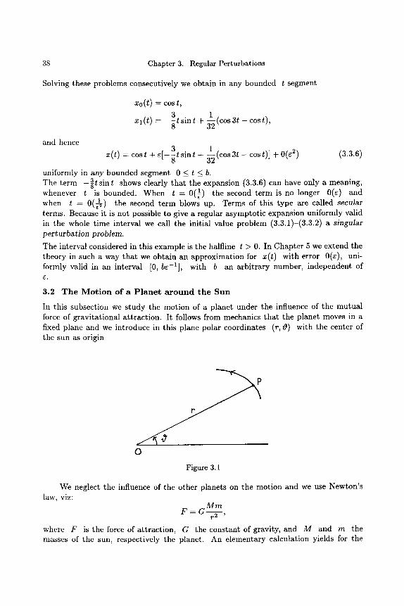
38 Chapter 3. Regular Perturbations
Solving these problems consecutively we obtain in any bounded t-segment
xo(t) = cost,
1 x l (t) = 3_t sin t + (cos 3t - cos t)
- 8 ~ '
and hence 1 x(t) = cost + e [ - 3 t s i n t + (cos 3t - cost)] + 0(e 2) (3.3.6)
8
uniformly in any bounded segment 0 _< t _< b. 3 sin t shows clearly tha t the expansion (3.3.6) can have only a meaning, The te rm - ~ t
whenever t is bounded. When t = 0(1) the second te rm is no longer 0(e) and when t = 0 ( ~ ) the second t e rm blows up. Terms of this type are called secular terms. Because it is not possible to give a regular asymptot ic expansion uniformly valid in the whole t ime interval we call the initial value problem (3.3.1)-(3.3.2) a singular perturbation problem. The interval considered in this example is the hairline t > 0. In Chapter 5 we extend the theory in such a way tha t we obtain an approximat ion for x(t) with error 0(e), uni- formly valid in an interval [0, be-i] , with b an arbi t rary number, independent of e .
3.2 T h e M o t i o n o f a P l a n e t a r o u n d t h e S u n
In this subsection we s tudy the mot ion of a planet under the influence of the mutua l force of gravi tat ional a t t ract ion. It follows from mechanics tha t the planet moves in a fixed plane and we introduce in this plane polar coordinates (r, 0) with the center of the sun as origin
P
J
O
Figure 3.1
We neglect the influence of the other planets on the motion and we use Newton's law, viz:
Mm F = G ~
r 2 '
where F is the force of a t t ract ion, G the constant of gravity, and M and m the masses of the sun, respectively the planet. An elementary calculation yields for the
3.2. The Motion of a Planet around the Sun 39
radial and the transverse components of the acceleration the formulae:
d2r ( d O ) 2 1 d ( d O ) ar dt 2 r --~ a # - - r - ~ r2
and so it follows from Newton's law of motion:
d2r ( d O ) 2 dt 2 r - ~ - - G
r 2 -- O. r dt - ~
M m r 2 ,
Integrat ing the second equation we obtain the second law of Kepler, i.e.
(3.3.7)
(3.3.8)
r 2dO -~- = h = constant , (3.3.9)
which means tha t the angular m o m e n t u m of the planet is constant. We put
1 ~(~) = ~(~),
where r - r(0) denotes the t ra jectory of the planet. We get the following relations
du _ du ~ d O _ 1 dr / h _ 1dr / / - , dO dt dt r 2 dt r 2 h dt
and
or with the aid of (3.3.7)"
o r
d2u d du ~ d O l d 2 r / h ,
dO 2 - dt ( - ~ ) -~ = h-dr ~ -~
d2u M m 1 dO 2 h 2 r
d2u M m + u = G ~
dO 2 h 2 �9
Finally, we introduce a characteristic distance ~ and the dimensionless variable - ~u; ~ satisfies the differential equat ion
d2~t
dO 2 - - - ~ - f i = a (3.3.10)
with a = G Mm~ h 2 �9
The solution is readily obtained and we get the result
= a + ( b - a)cos(O - O0), (3.3.11)
40 Chapter 3. Regular Perturbations
where the constants b and ~0 are determined by the initial conditions, which specify the position and the velocity of the planet when e.g. v9 = 0.
It follows tha t r (0) is given by
r(vq) = a + (b - a )cos(~ - 0o) (3.3.12)
and the t ra jectory of the planet is for b < a a fixed ellips with the centre of the sun at one of its loci. However, observation has revealed tha t the major axis of the ellips rotates slowly around the sun and so the result (3.3.12) is not completely correct. It was a verification of Einstein's theory of gravity tha t this rotat ion could be explained by using the theory of general relativity and the so-called Schwarzschild metric (see e.g. [7], Ch.XIV). In this theory the equation (3.3.10) should be replaced by
d2'5 d,02 t- '5 - a + ~'52 (3.3.13)
with e---- 3 G M m c2e , c the velocity of light, and so 6 is a small positive number.
Therefore we are led again to a per turba t ion problem which can be handled in the same way as the nonlinear spring. The equation (3.3.13) is supplemented with the initial conditions
d'5 '5(0) -- c~, ~-~ (0) -- ,6. (3.3.14)
Applying the theory of this chapter we make the assumption
~(~) = u0(O) + ~ , ( ~ ) + . . . + ~"u.(O) + . . . (3.3.15)
Subst i tut ion into (3.3.13) and collecting the terms with equal powers of e we get a linear system of recurrent initial value problems for the functions ui(tg), i - 0, 1, 2 , . . .
d2uo duo d0--- 5- + u0 = a, u0(0) - c~, - -~ (0 ) --/3 (3.3.16)
d2ul dul dO---- 5- + ul = u20, ul(0) = 0, --d-~(0) = 0 (3.3.17)
Solving these problems consecutively we obtain:
Uo(O) : a + (o~ - a)cos vq + ~ sin z9 d d
ul (~) = sin 0 / [ u o (~o)] 2 cos ~od~o - cos ~ / [ u o ( ~ ) ] 2 sin ~d~o
o o
= a(c~ - a)O sin 0 - afh9 cos 0 + . . . .
(3.3.18)
(3.3.19)
Exercises 41
According to Theorem 3.3.1 we have the result
~(~) = ~0(~) + ~ (~) + 0(~ ~) (3.3.20)
uniformly in any bounded domain, say o < ~ < t~b, with Zgb independent of ~.
We see again the appearance of "secular" terms ~)sin zg, t9 cos~9 in the contribution cul (v~), and thereforethe expansion (3.3.20) is only meaningful in bounded ~9-intervals.
In the next chapter we explain as a consequence of (3.3.20) the perihelium rotation and in Chapter 5 we extend the range of uniform validity.
E x e r c i s e s
1. Let y(x; ~) be the solution of the initial value problem
dy = l + y 2 + r x > 0 , y ( 0 ) = r 0 < ~ < < 1 ,
dx
valid in a right neighbourhood of x = 0. Give an approximation of y(x; ~) within an error O(~ 2) and its interval of uniform validity.
2. Let y+ (t; c) be the solution of the initial value problem
d2y+ + dy+ dy+ dt 2 - - ~ + y + = 0 , t > 0 , y + ( 0 ) = 0 , - - ~ ( 0 ) = 1 ,
with 0 < ~ < < 1 . Give by using the regular expansion method an approximation of y+ (t; c) within an error O(~ 2) and its t-interval of uniform validity. Discuss the reason why the result is not satisfactory.
3. Consider the Duffing initial value problem with a small forcing term
d2u du dr---- ~ + u - - - f u 3 -~- eA cos t, t > O, u(O) -- 1, -d-~-(O) = O, 0 < ~ ~ 1.
For which values of the amplitude A is the resonance only observable in the third term of the asymptotic approximation?

This Page Intentionally Left Blank
Chapter 4
T H E M E T H O D OF T H E S T R A I N E D C O O R D I N A T E
1. I n t r o d u c t i o n
In the preceding chapter we showed that the naive regular perturbation method has the severe restriction that it is only applicable for finite time intervals and so we cannot construct by this method asymptotic approximations uniformly valid in "large" time intervals, that is to say for intervals of e.g. O(~) or even for all values of t > 0. This becomes apparent in the occurrence of secular terms; see the examples of the nonlinear spring and the motion of a planet.
Nevertheless, by using a modification of the regular perturbation method involving a stretching of the time coordinate as
t - ( 1 + ewl + e2w2 + ' ' ' )T (4.1.1)
it is possible to determine the constants {wi} such that the solution of the perturbed differential equation does no longer contain secular terms; in this way one obtains an asymptotic expansion valid for time intervals of O(~). With the aid of this modification it is also possible to obtain information on certain important quantities such as for instance the frequency of the nonlinear spring and the perihelium precession of the planet. The method of straining the coordinate originates from Lindstedt [98, 99] and Poincar~ [116], who introduced it in studies of perturbation problems in celestial mechanics. Therefore it is also called the Lindstedt-Poincard or shortly the L.P.-method. We il- lustrate the method by treating again the nonlinear spring and the motion of a planet around the sun. The question of the asymptotic correctness of the Lindstedt-Poincard procedure will be dealt with in the next chapter. We conclude this chapter with a pro- cedure introduced by Lighthill [96, 97], who generalized the stretching transformation (4.1.1) by setting
t -- T + e f l ( T ) + e2f2(T ) + . . . , (4.1.2)
where the stretching functions {fi} are chosen such that an asymptotic expansion of the solution of the perturbation problem becomes possible. This transformation appears to be useful for a class of perturbation problems for which the reduced differential equation with e - 0 contains a singularity, e.g. (t -1 t- "CU)du + q( t )~ = ~(t) , t > o.
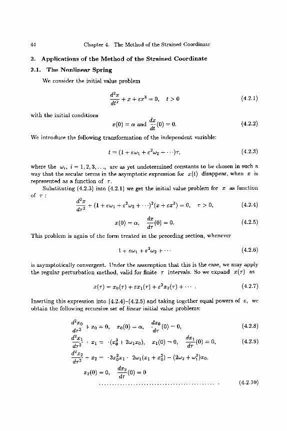
44 Chapter 4. The Method of the Strained Coordinate
2. A p p l i c a t i o n s of t h e M e t h o d of the Strained Coordinate
2.1. The Nonl inear Spring
We consider the initial value problem
d2x dt 2 t - x + ~ x 3 = 0 , t > O (4.2.1)
wi th the initial conditions dx
x(0) = a and -~- (0) = 0.
We introduce the following transformation of the independent variable:
(4.2.2)
t = (1 + ewl + e2w2 + " ' ) % (4.2.3)
where the w~, i - 1, 2, 3 , . . . , are as yet undetermined constants to be chosen in such a way that the secular terms in the asymptotic expression for x( t ) disappear, when x is represented as a function of r.
Substi tuting (4.2.3) into (4.2.1) we get the initial value problem for x as function of T :
d2x dT---- ~ -~- (1 + ewl + g2w2 -~- - - ' )2 (x -[- Ex 3) -- 0, T > 0, (4.2.4)
dx x(0) = c~, ~--~T (0) = 0. (4.2.5)
This problem is again of the form treated in the preceding section, whenever
1 + ewl + e2w2 + " " (4.2.6)
is asymptotically convergent. Under the assumption that this is the case, we may apply the regular per turbat ion method, valid for finite T intervals. So we expand x(~-) as
~(~) = ~0(~) + ~ ( ~ ) + ~ ( ~ ) + - (4.2.7)
Inserting this expression into (4.2.4)-(4.2.5) and taking together equal powers of e, we obtain the following recursive set of linear initial value problems:
d2xo dxo a~---3- + ~o = o, ~o(O) = ~, - ~ j ( o ) = o,
d 2 x 1 dx 1 dT_----- Y -f- xl = -(Xo 3 + 2wlxo), xl(0) = 0, --~-T (0) = 0,
d2x2 dT--- Y + x2 = - -3x2x , -- 2w1(x1 -[- XO 3) -- (2~2 -[-W12)Xo,
dx2 ~ ( o ) = o, -jj~ (o) = o
. . . . . . . . . . . . . . . . . . . . . . . . . . . . . . . . . . . . . . . . . . . . .
(4.2.8)
(4.2.9)
(4.2.10)
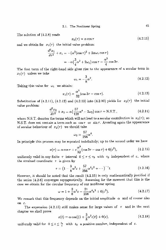
2.1. The Nonlinear Spring 45
The solution of (4.2.8) reads x0(r) = a c o s T (4.2.11)
and we obtain for Xl(T) the initial value problem:
d2xl d ~ + ~1 = - { ~ ( ~ o s ~) ~ + 2 ~ 1 ~os~}
C~ 3
(_3 62 2wl) T -- --4 cos 3T. - - c ~ , , 4 + cos
The first term of the right-hand side gives rise to the appearance of a secular term in x l (T) unless we take
3 2 (4.2.12) CO 1 DE O~ . 8
Taking this value for W 1 we obtain: C~ 3
Xl(T) = ~--~(cos 3T - COST). (4.2.13)
Substi tution of (4.2.11), (4.2.12) and (4.2.13)into (4.2.10) yields for X2(T) the initial value problem:
d2X2dT 2 (~57 ~ 4 _ 2 w 2 ) C O S T + N.S.T., (4.2.14) + x2 = a ~ l ~ g
where N.S.T. denotes the terms which will not lead to a secular contribution in x2(T); so N.S.T. does not contain a term such as cos T or s in T. Avoiding again the appearance of secular behaviour of X2(T) we should take
092 --- 57.64" 256
In principle this process may be repeated indefinitely; up to the second order we have
OL 3 X(T) = a cos T + C~-~ (COS 3T -- COS T) + 0(~2), (4.2.15)
uniformly valid in any finite T interval 0 _< T _< TO with TO independent of ~, where the strained coordinate T is given by
57 o4c 2 -~-'-' ) - i t . (4.2.16) T = (1 - c~2~ + 256
However, it should be noted that the result (4.2.15) is only mathematical ly justified if the series (4.2.6) converges asymptotically. Assuming for the moment that this is the case we obtain for the circular frequency of our nonlinear spring
_3 21 O4e 2 -~-0(e3) . (4.2.17) w = 1 + 8 6 2 ~ - 256
We remark that this frequency depends on the initial amplitude a and of course also on ~ ' .
The expression (4.2.15) still makes sense for large values of T and in the next chapter we shall prove
3626)t} + 0(~), (4.2.18) x( t ) = a cos{(1 + g
uniformly valid for 0 < t < to with to a positive number, independent of ~.
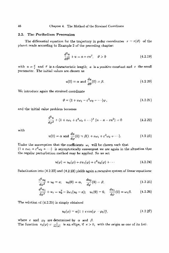
46 Chapter 4. The Method of the Strained Coordinate
2.2. T h e P e r i h e l i u m P r e c e s s i o n
The differential equation for the t ra jectory in polar coordinates r - r (0) of the planet reads according to Example 2 of the preceding chapter:
d2u dO--- ~ + u = a + eu 2, 0 > 0 (4.2.19)
with u = ~ and ~ is a characteristic length; a is a positive constant and e the small parameter . The initial values are chosen as
du u(O) = cr and ~-~(0) = ft. (4.2.20)
We introduce again the strained coordinate
0 = (1 + ewl + e2w2 + ' " ) 9 ~ , (4.2.21)
and the initial value problem becomes
d2u
d~p 2 + (1 + COd I + ~2~d 2 ~ - ' " .)2 (U -- a -- Cu 2) ~- 0 (4.2.22)
with du
u(0) = a and - 7 ( 0 ) = fl(1 + ewl + e2w2 + ' " "). aT
(4.2.23)
Under the assumption tha t the coefficients wi will be chosen such tha t (1 -Jr CO) 1 -~ E2W2 - ~ ' - . ) is asymptot ical ly convergent we are again in the si tuat ion tha t the regular per turba t ion method may be applied. So we set
u(~) = ~0(~) + ~Ul(~) + ~ ( ~ ) + . . . (4.2.24)
Subst i tut ion into (4.2.22) and (4.2.23) yields again a recursive system of l inear equations:
d2u______oo _ duo u0 = a; u0(0) = a, - ~ - (0) = fl, dT 2
d2ul + u~ = u0 ~ - 2 ~ 1 ( u 0 - ~) ; ~ ( 0 ) = 0, d~ 2
(4.2.25)
dltl -d~ (0) =Wlfl . (4.2.26)
The solution of (4.2.25) is simply obtained
UO(T) = a{1 + e cos(qo -- (P0)}, (4.2.27)
where e and ~o0 are determined by a and /3. The function r0(T) = 1 ~o(~) is an ellips, if e > 0, with the origin as one of its loci.
3. The Method of the Strained Parameter 47
Substitution of u0(cp) in the right-hand side of the differential equation (4.2.26) yields
d2Ul d~o------- 5- + u: -- a2(1 + le2) + 2ae(a - w:)cos(~o - ~Oo)
+ l a 2 e 2 cos 2 ( ~ 0 - qo0). 2
This equation gives again rise to a secular term unless we take
wl - a. (4.2.28)
Therefore we get u = a + ae cos(~o - ~o) + 0(:),
uniformly in any bounded ~ interval 0 ~ ~ < 9~0 with
q:, = (1 + a: + w2:2 + . . . ) - 1 0 .
This process may, in principle, be repeated indefinitely and the asymptotic approxima- tion is valid if the series 1 + a : + 022:2 -~- "'" is asymptotically correct. Assuming the lat ter condition we have finally
u(O) -- a + ae cos{(1 - ae)O - 0o} + 0(:), (4.2.29)
uniformly valid for 0 < 0 _ t~ b with 0 b an arbitrary positive number independent of
In the next chapter we shall prove the asymptotic correctness of (4.2.29), which is even uniformly valid for 0 < 0 < o__~b with ~qb again some positive number, independent of :.
The peri- and aphelium of the planet is obtained for the values 0 -- Op with
du
dO
- - 0 (u is maximal, respectively minimal)
i.e. 0p satisfies approximately the relation sin{(1 - a : ) O p - 00} = 0, and it follows that (1 - a:)vqp -- t90 + 7rn, n = 0, 1, 2. Two consecutive values of the perihelium angle differ 2, y : ~ ~ 21r + 21ra:, and so the perihelium precession is approximately given by the formula
G 2 M 2 m 2 2~ra: - 6 1 r ~ . (4.2.30)
c2h 2
3. T h e M e t h o d of t h e S t r a i n e d P a r a m e t e r
It may happen that in a differential equation, apart from the small parameter e, another parameter, say p, appears which depends on :, but this dependence is quanti tat ively unknown. The requirement of a certain behaviour of the solution of the differential equation, e.g. no secular terms should be present, may lead to an asymptotic
48 Chapter 4. The Method of the Strained Coordinate
expansion of the parameter p into powers of e. The method for obtaining an asymptot ic approximat ion for as well the solution as for the unknown parameter is sometimes called the method of the strained parameter . We give as an illustration the following example. Stokes [147, p.486] considered in 1849 weakly nonlinear wave propagat ion on the surface of a liquid. His model is one dimensional and the height u ( x , t) of the fluid measured from equilibrium satisfies an equation of Klein-Gordon type
utt - o~2uxx -~- ,),2~t = /~u 3, (4.3.1)
where a, /~ and 7 are certain constants. We are interested in obtaining the so-called dispers ion re la t ion for p e r i o d i c t rave l l ing waves; the dispersion relation relates the wave number and the frequency.
The linear case with fl = 0 is almost trivial. Pu t t ing
u = u(~) , ~ = x - ct, (4.3.2)
with c > c~ > 0 the wave velocity, we get for u(~) the ordinary differential equation:
(c 2 - a2)u '' + 72u = 0,
and it follows tha t u(~) is a linear combination of sin{ 7 ( x - c t ) } and ~/c 2 --0~ 2 cos{ . . . 7 ( x - ct)}, and so the wave number is given by
~/C 2 -- Ot 2
k= 7 X/C -- C~ 2
and hence w 2 = k2c 2 = a2k 2 + 72, (4.3.3)
which relates the wave number k and the frequency w. It is to be noted tha t this relation is independent of the ampli tude of the wave.
We consider now the full nonlinear equation, which reads
(C 2 -- O~2)U t ' ~- ') '2U = ~ U 3 ( 4 . 3 . 4 )
with u = u(~) = u ( x - ct).
We assume tha t the ampli tude a of the wave is small and so we put
u = aft (4.3.5)
and there results (c 2 - a2)~" % 72fi - ~a2fi 3, (4.3.6)
and this would present again a per turba t ion problem of the kind considered before with a 2 instead of e, whenever the wave velocity were to be independent of the amplitude. But as is well known from nonlinear wave phenomena the speed of the wave depends on the ampli tude. Because a is small we expand c into powers of a
C -- CO + acl A- a2c2 + ' ' ' , (4.3.7)
3. The Method of the Strained Parameter 49
where the coefficients c~ should be chosen properly with co > c~. We bring (4.3.6) into the form
~" -V2~2 + ~a2u3 (4.3.8) U - -
c 2 _ o l 2
and we expand c2_1~2 into powers of a. If the series (4.3.7) converges asymptot ical ly we are again in the si tuat ion of Chapter 3 and we may apply the regular per turba t ion method. We assume now tha t (4.3.7) is indeed asymptot ical ly correct and we put
~(~) = ~1 (~) + a~2(~) + a2~3(~) + " " (4.3.9)
or what amounts to the same
u(~) = aul(~)+ a2u2(~) + a3u3(~) + " " �9 (4.3.10)
Instead of subst i tut ing (4.3.9) and (4.3.7) into (4.3.8) and taking together equal powers of a, we may as well subst i tute (4.3.10) and (4.3.7) directly into equation (4.3.6). Taking together equal powers of a, there results the following recursive set of linear equations for the functions ui(~), i = 1, 2 , . . . .
(~] _ ~2)~, + ~ 2 ~ = 0
(~ - ~ ) ~ + ~ = - 2 ~ o ~
(~0 ~ ~ ) u g + ~ ( -2~o~ ~' " " Z ~ . - - - - - - C l ) U 1 - - 2 C o C l U 2 - 'k
(4.3.11)
(4.3.12)
(4.3.13)
We star t with a par t icular solution of (4.3.11), viz.
~1 = cos(k~) (4.3.14)
with k 2 _ ,)12
- c2 _ a2 or c~ = c~ 2 + ~'2k-2, (4.3.15)
which corresponds with the dispersion relation (4.3.3) for the linear case with fl = 0. We subst i tute Ul(~) into (4.3.12) which gives
, 2c0cl k2 u~. + k2u2 = Co ~ _ ~ . cos(k~).
Searching for waves a2u2 of small ampli tude we should eliminate secular terms and so we must take Cl - 0 and the equation for u2 becomes the same as tha t for ul �9
The equation for u3 becomes now
~ cos(3k~) ,, 1 (2coc2 k2 + p) cos(k~) + 4(c2 c~2) U 3 ~ k 2 u 3 - - c ~ - oz 2 - "
Eliminat ing the secular te rm again we should take
3 2coc2 k2 -~- -:~ = 0, or c2 --
4
3p 8 c o k 2
(4.3.16)
50 Chapter 4. The Method of the Strained Coordinate
and the differential equation for u3 reduces to
" f~ cos(3k~). (4.3.17) u3 + k~u3 = 4 ( ~ - ~)
Under the condition that (4.3.7) is asymptotically correct, i.e.
c - c o -4- a2c2 + 0(a 3) - Jo~ 2 A- ~,2]~2 _ 3~a2 8k 2 J ~ 2 ~_ ~,2k-2 -4- O(a 3)
we have obtained the approximation
u ( x - ct) = a cos k ( x - ct) + O(a2). (4.3.19)
with the dispersion relation
= kc = V/c~2k 2 + 72 - 3f~a2 + O(a3). (4.3.20) 8 j ~ 2 k 2 A- ,72
The dependence of w on the amplitude appears to be only quadratic. It is not difficult to integrate (4.3.6) directly; multiply with fi', integrate and one obtains u as an elliptic function of ~, (cnoYdal wave). Taking the amplitude small one arrives at a result similar as (4.3.20); see also [147], p.486-489.
4. L igh th i l l ' s m e t h o d
An interesting class of perturbation problems concerns the case where the reduced equation with ~ = 0 is singular while the perturbed equation is not singular. A typical perturbation problem of this type is
(x + r du -~x + q ( x ) u = r ( x ) , 0 < x _< 1, (4.4.1)
with u ( 1 ) = b and q and r smooth functions, q(O)# O. Using the Poincar6-Lindstedt method the uniformity of an asymptotic expansion does not hold in a neigbourhood of x - O . Put t ing
x = (1 + eWl + ~20.'2 + ' " ")~
~(~) = ~0(~) + ~u~ (~) + ~ ( ~ ) +. . . leads to the recursive set of singular linear differential equations
~ - - ~ + q ( ~ ) u , = f , ( ~ , uo, u l , . . . , Un--1)~
with solutions not suitable in the expansion of u(~) in the neighbourhood of ~ = 0. To illustrate this situation consider the very simple example
( z + r du - - ~ x + U - - O , O < x < l , u(1)---1, 0 < r (4.4.2)
4. Lighthill's method 51
This equat ion may be wri t ten as a Hamil ton-system
with the solution
o r
dx du .-7 = (x + 6u), ,-7 = - u , u(1) = 1 (4.4.3) qa ga
- x + Vrx 2 + 26 + e 2 u = . (4.4.4)
6
This solution is regular in x for all values of x with x _ 0 and for all positive values of 6, but it has only for x > 5 > O, with 5 independent of 6, the asymptot ic relation u - s + 0(6) . Let us now make the straightforward expansion x
= ~o(~) + ~ ( ~ ) + . . . . (4.4.5)
Subst i tut ion into (4.4.2) yields after equat ing coefficients of equal powers of e o and 61"
and therefore
duo x--~x + u 0 - - - 0 , u 0 ( 1 ) = l ,
dul duo x - ~ - x + Ul = - u o - ~ - x , Ul(1) = O,
1 1 u 0 = - a n d u l = ( 1 - x -2)
The te rm u0 is singular and Ul is even more singular at x -- 0 and so the regular expansion procedure is useless in the neighbourhood of x - 0. The stretching of the coordinate x according to
x = (1 + ~W 1 ~- 82W 2 - ~ ' " ")~ (4.4.5)
is, of course, of no help since x is only multiplied by a factor of O(1). Lighthill [96, 97] devised a generalization of the coordinate stretching (4.4.5) such tha t the singularity no longer occurs in the expansion. Instead of the simple linear coordinate t ransformation, he introduced the t ransformat ion
- ~ + ~f~(~) + e2f2(~) + . . . (4.4.6)
where now the straining functions fi(~) of class C ~ are chosen such tha t as well
~(~) = ~0(r + ~ ( r + ~ 2 ( r + . . - (4.4.7)
as (4.4.6) become both uniform expansions in the domain considered, in our example 0 < x < 1. This is guaranteed by the requirements tha t
um(~c) and fm(~c) (4.4.8) u~_~(~) f~_~(~)
52 Chapter 4. The Method of the Strained Coordinate
are uniformly bounded in the ~-interval corresponding with the x-interval [0, 1]. Despite the fact that the method is cumbersome and involves many tedious cal-
culations, it has been applied in a large variety of perturbation problems concerning wave propagation; we refer the reader to an extensive list in the book by Nayfeh, [108, p.78, 79]. Therefore we illustrate the procedure using the simple example above, which was also given by Tsien [135]. Substitution of (4.4.6) into (4.4.2) gives
du {(: + :::(:) + :s,(:) +.-.) + : u } : +
df l ..c2 df 2 {1 + e-d-~-(~ ) + -d-~-(~) + . . . }u = o, (4.4.9)
and substitution of (4.4.7) into (4.4.9) yields as before a recursive system of / /near differential equations:
d d~ (~u0) = 0
d d duo ~ ( ~ 1 = - ~ ( S ~ o ) - ~0 d~
(4.4.10)
(4.4.11)
To get the boundary conditions it is necessary to invert the expansion (4.4.6); we have to find the expansion of ~ = ~*, the value of which corresponds with the value x - 1. In other words, we should construct a root of the equation
1 = ~* + 6fl (t~*) + e2f2(~ *) + - - " �9 (4.4.12)
Its approximate solution is obtained with the aid of the regular perturbation method, i.e. we assume
~* = 1 + ble + b2e 2 + " " (4.4.13)
and insert this into (4.4.12):
(bl~ + b2~ 2 + - - ' ) q- {~.fl (~*) q- ~2f2(~*) + ' " "} = 0. (4.4.14)
Expanding fi(~*) into a Taylor expansion around ~ = 1 we have
f~(~*) -- fi(1) + f~(1)(bl~ + b2c 2 + . . . ) + 1f~'(1)(b16 + b262 + " ' ) 2 + . . . ,
and (4.4.14) becomes
(bl~ + b2~ 2 + ' " ") + ~{fl(1) + f~(1)(bl~ + b2 ~2 + ' " ") + ' " "}
+ ~{f~(1) + A(1)(b: + b: ~ + ) +.--} + ................................... --0.
4. Lighthill's method
Taking finally equal powers of 6 together we get
bl = - f l ( 1 )
b2 -- -b l f~ (1) - f2(1) - f l (1)f~(1) - f2(1) . . . . . . . . . . . . . . . . . . . . . . . . . . . . . . . . . . . . . .
and so there results formally
~* = 1 - ef l (1) + e2{fl(1)f~(1) - f2(1)} + " " �9
The boundary condition ux=l = u(~*) = 1 becomes
uo(~*) + eUl (~*) + e2u2(~c*) + . . . . 1
o r
53
(4.4.15)
Ul(1) = u~)(1)f(1), . . . . (4.4.16)
1 u0(~) = ~, (4.4.17)
and the boundary value problem for Ul(~) becomes according to (4.4.11) and (4.4.16)
d 1 1 1 dfl d--~(~ux) = ~-5 + ~-~f l (~) - ~ - ~ ( ~ ) (4.4.18)
with u~(1) = - f1 (1 ) . (4.4.19)
From the equations (4.4.10)-(4.4.11) it follows after multiplication of the first with U l and of the second with u0 and subtract ion tha t
d ( u l ) l(dfl fl 1)
pertaining to (4.4.10), (4.4.11 ) ....
u0(1) = 1,
The solution of (4.4.10), (4.4.16) is
uo(1) + u~(1){ - ef l (1) + e2(fl(1)f;(1) - f2(1)) + ' " }
1 e2 + ~u~(1){ - e l l ( l ) + ( f l (1 ) f l (1 ) - f2(1)) + " " }2
. . . . . . . . . . . . . . . . . . . . . . . . . . . . . . . . . . . . . . . . . . . . . . . . . . . . . . . .
+ C[Ul(1) + u~(1)( - e l l ( l ) + c2( f l (1 ) f ; (1 ) - f2(1)) + ' " }
1 "(1)( - ef l (1)+ e2(fl(1)f~(1)- f2(1)) + . . . }2 + ~ul
. . . . . . . . . . . . . . . . . . . . . . . . . . . . . . . . . . . . . . . . ", . . . . . . . . . . . . . . . ]
+ (1) + . . . . . . . . . . . . . . . . . . . . . . . . . . . . . . . . . . . . . . . . . . . . ]
+ . . . . . . . . . . . . . . . . . . . . . . . . . . . . . . . . . . . . . . . . . . . . . . . . . . . . . 1.
Taking again equal powers of c together, we get the recursive set of boundary conditions
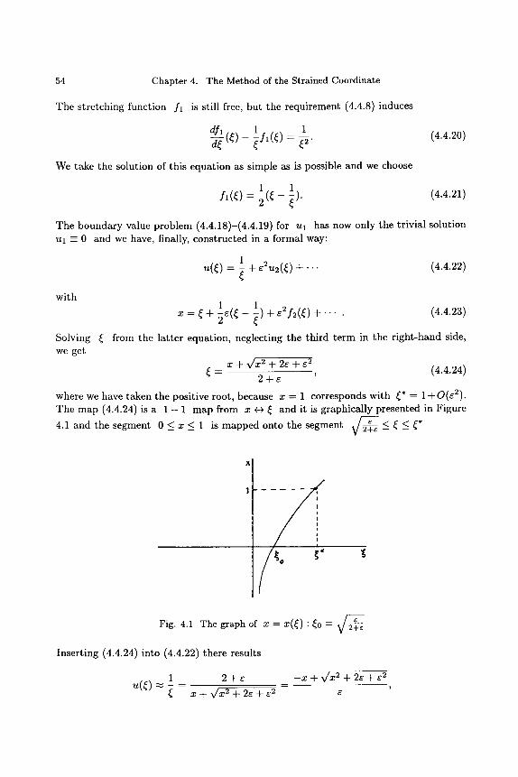
54 Chapter 4. The Method of the Strained Coordinate
The stretching function f l is still free, but the requirement (4.4.8) induces
dfl 1 1 (4.4.20) d~
We take the solution of this equat ion as simple as is possible and we choose
1 1 f l (~) = ~ ( ~ - ~). (4.4.21)
The boundary value problem (4.4.18)-(4.4.19) for Ul has now only the trivial solution u l - 0 and we have, finally, constructed in a formal way:
1 u(~) = ~ -~- e2u2(~) -~- .- . (4.4.22)
with
x : ~ + e ( ~ - ~ ) + e 2 f 2 ( ~ c ) + . . . . (4.4.23)
Solving ~c from the la t ter equation, neglecting the third t e rm in the r ight-hand side, we get
x + ~/x 2 + 2E + ~2 = , (4.4.24)
2 + ~
where we have taken the positive root, because x = 1 corresponds with ~* = 1+O(e2) . The map (4.4.24) is a 1 - 1 map from x +-> ~c and it is graphically presented in Figure
,I ~ <~ <~* 4.1 and the segment O_<x_< 1 is mapped onto the segment ~ _ _ V
/
Fig. 4.1 The graph of x = x(~C) �9 ~C0 -- ~/ e 2u v
Insert ing (4 .4 .24) into (4.4.22) there results
1 2 + ~ - x + ~/x 2 + 2e + ~2
u ( ~ ) ~ ~ = ~ + J ~ + 2~ + ~ =
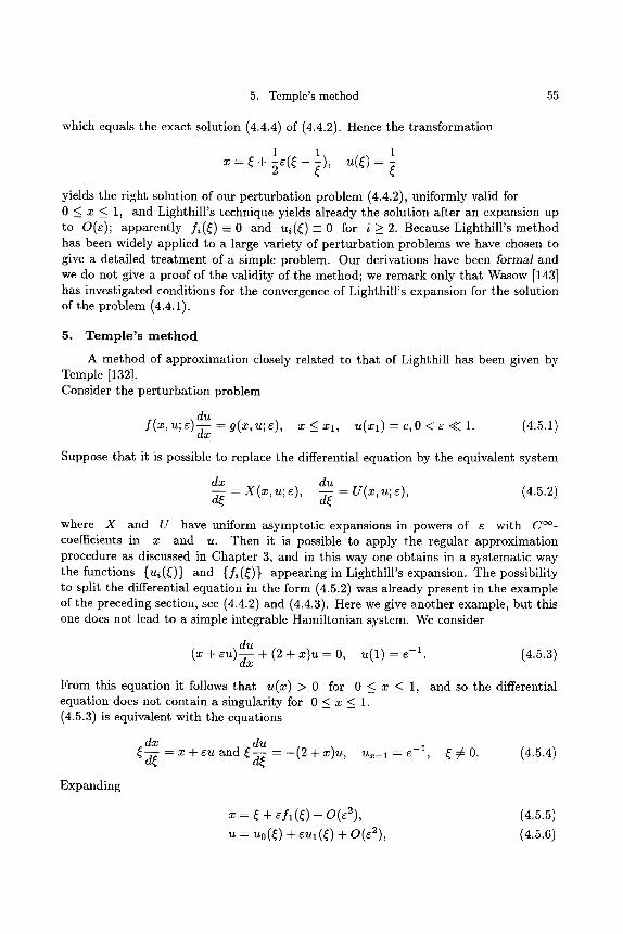
5. Temple's method 55
which equals the exact solution (4.4.4) of (4.4.2). Hence the transformation
1 1 1 - ~ + ~ ( ~ - ~), u(~)=
yields the right solution of our perturbation problem (4.4.2), uniformly valid for 0 __ x _< 1, and Lighthill's technique yields already the solution after an expansion up to O(~); apparently f i ( ~ ) = 0 and u i ( ~ ) - O for i > 2. Because Lighthill's method has been widely applied to a large variety of perturbation problems we have chosen to give a detailed treatment of a simple problem. Our derivations have been formal and we do not give a proof of the validity of the method; we remark only that Wasow [143] has investigated conditions for the convergence of Lighthill's expansion for the solution of the problem (4.4.1).
5. Temple ' s m e t h o d
A method of approximation closely related to that of Lighthill has been given by Temple [132]. Consider the perturbation problem
f (x, u;-c) du - g(x ,u;~) , X < Xl, U(Xl)-C, 0 < c < < l . (4.5.1)
Suppose that it is possible to replace the differential equation by the equivalent system
dx du = X ( x , u; ~), -w~ = U(x, u; c), (4.5.2)
d~ a~
where X and U have uniform asymptotic expansions in powers of e with C ~- coefficients in x and u. Then it is possible to apply the regular approximation procedure as discussed in Chapter 3, and in this way one obtains in a systematic way the functions {ui(~)} and {fi(~)} appearing in Lighthill's expansion. The possibility to split the differential equation in the form (4.5.2) was already present in the example of the preceding section, see (4.4.2) and (4.4.3). Here we give another example, but this one does not lead to a simple integrable Hamiltonian system. We consider
(x + cu) du dxx + ( 2 + x ) u = 0 ' u ( 1 ) - e -1. (4.5.3)
From this equation it follows that u(x) > 0 for 0 _< x _< 1, and so the differential equation does not contain a singularity for 0 _< x _< 1. (4.5.3) is equivalent with the equations
dx du - (2 + x)u, ~ - ~ + ~ n d ~ =
Expanding
Ux-- 1 - - e -1, ~ ~: 0. (4.5.4)
= ~ + ~I~ (r + o ( ~ ) ,
= ~0(~) + ~u, (~) + o ( ~ ) ,
(4.5.5)
(4.5.6)
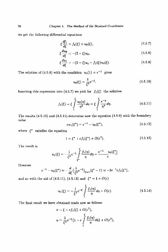
56 Chapter 4. The Method of the Strained Coordinate
we get the following differential equations
dYl ~-d-~- -- f l ( ~ ) + u0(~) , (4 .5 .7)
duo - (2 + ~)u0, (4.5.8) ~-d~- :
dul - (2 -]-~)tt 1 -- f l (~)u0(~). (4.5.9) ~ - ~ =
The solution of (4.5.8) with the condition uo(1) = e -1 gives
1 (4.5.10) ~0(~) : ~2 ~-~"
Inserting this expression into (4.5.7) we pick for f l ( ( ) the solution
f l (~) -- ~ dr/= ~ ~ d r / . (4.5.11)
1 1
The results (4.5.10) and (4.5.11) determine now the equation (4.5.9) with the boundary value
~U 1(~*) : e -1 -- ItO(~*), (4 .5 .12)
where ~* satisfies the equation
1 = (* + el l (~*) + O(e2). (4.5.13)
The result is
1 e- ( f f l (77) u:(:) = - ~ dr/+ e - I __ UO(~* )
However -1 c - - - - e ) ( = 1 ( ~ - - 1) , ~ - 3 e - e / l ( ~ * ) ,
and so with the aid of (4.5.11), (4.5.13) and ~* = 1 + O(e)
1 _~ f fl(r/) dr/+ O(e). Ul(~) = --~-~e r/ 1
The final result we have obtained reads now as follows:
x -- ~ A- ~ f l (~) -f- O(~2) ,
J f l (r/) 1 _~ (1 e dr/) -~- O(g'2), U = ~--~e -- r/ 1
(4.5.14)
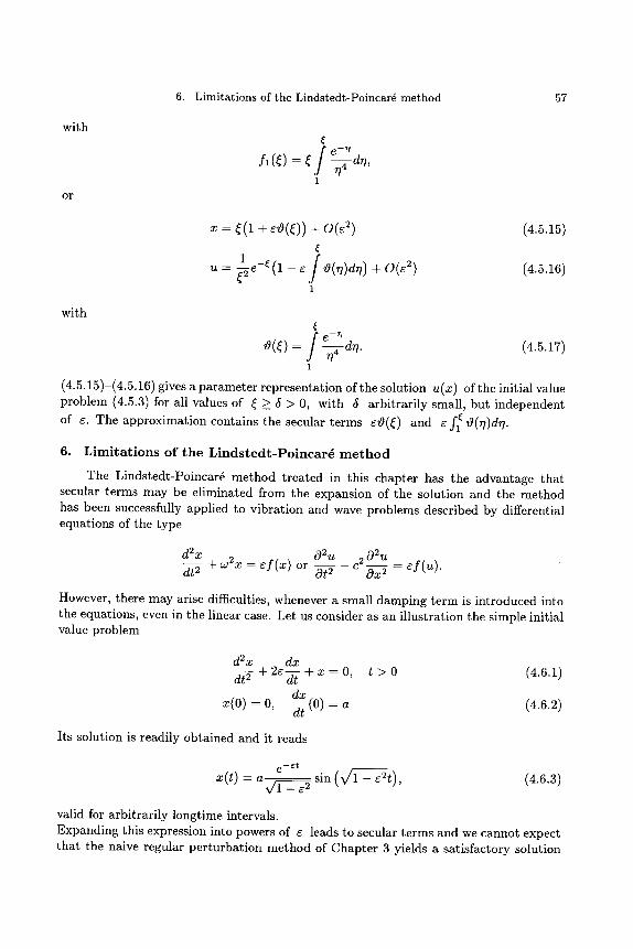
6. Limitations of the Lindstedt-Poincar~ method 57
with
o r
f e-~ .f~ (r = ~ --~-dn, 1
x - ~(1 + e~(~)) + O(e 2) (4.5.15)
1 -~(1 e / u = ~-se - O(~)drl) + O(e 2) (4.5.16)
1
with
f e--rb ~(~) - --~- dr/. (4.5.17)
1
(4.5.15)-(4.5.16) gives a parameter representation of the solution u(x) of the initial value problem (4.5.3) for all values of ~ _> 5 > 0, with 5 arbitrarily small, but independent
of e. The approximation contains the secular terms eO(~) and e f : ~)(r/)dr/.
6. L i m i t a t i o n s of t h e L i n d s t e d t - P o i n c a r 6 m e t h o d
The Lindstedt-Poincar6 method treated in this chapter has the advantage that secular terms may be eliminated from the expansion of the solution and the method has been successfully applied to vibration and wave problems described by differential equations of the type
d2x dt 2
0 2 u _ c 2 0 2 u + w2x -- ~ f ( x ) or - ~ ~ x 2 -- ~f (u ) .
However, there may arise difficulties, whenever a small damping term is introduced into the equations, even in the linear case. Let us consider as an illustration the simple initial value problem
d2x dx + 2e-~. + x = O ,
dt---- ~ dx
x(O) - O, --~(0) = a
Its solution is readily obtained and it reads
t > 0 (4.6.1)
(4.6.2)
- - e t e x( t ) = a-~/1 _ e 2 sin (V/1 - s2t), (4.6.3)
valid for arbitrarily longtime intervals. Expanding this expression into powers of r leads to secular terms and we cannot expect that the naive regular perturbat ion method of Chapter 3 yields a satisfactory solution
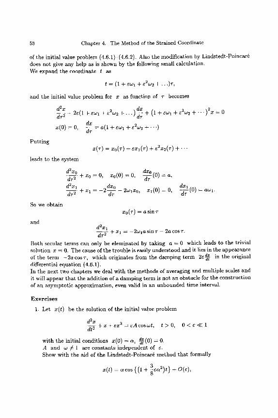
58 Chapter 4. The Method of the Strained Coordinate
of the initial value problem (4.6.1)-(4.6.2). Also the modification by Lindstedt-Poincard does not give any help as is shown by the following small calculation. We expand the coordinate t as
t = (1 + r + e2ca2 + . . . ) T ,
and the initial value problem for x as function of T becomes
d2x dx dT 2 -[- 2e(1 + r + g2ca2 -~-" "")dT ~- (1 + gcal -~- g2ca2 -~-'" ") 2x = 0
dx = a(1 + ewl + r -f-'" ") �9 (o) = o,
Put t ing
leads to the system
~(~) = ~0(~) + ~ 1 ( ~ ) + ~ ( ~ ) + . -
d2xo dxo dT---- ~ + x0 = 0, x0(0) -- 0, -~T (0) -- a,
d2xl ~dxo dxl (0) d~---~ + ~ = - z - j V - 2~1~0, ~ ( 0 ) = 0, ~ = ~ 1 .
So we obtain Xo(T) -- a sin T
and d2xl
+ x 1 -- - 2cala sin r - 2a cos r. dT 2
Both secular terms can only be eleminated by taking a = 0 which leads to the trivial solution x - 0. The cause of the trouble is easily understood and it lies in the appearance
ax in the original of the term - 2 a cos T, which originates from the damping te rm 2e 2? differential equat ion (4.6.1). In the next two chapters we deal with the methods of averaging and multiple scales and it will appear tha t the addit ion of a damping term is not an obstacle for the construction of an asymptot ic approximation, even valid in an unbounded t ime interval.
Exercises
1. Let x(t) be the solution of the initial value problem
d2x
dt 2 + x + e x 3 = e A c o s w t , t > 0 , 0 < e < < l
dx with the initial conditions x ( 0 ) = a, ~ - ( 0 ) = 0. A and ca # 1 are constants independent of v. Show with the aid of the Lindstedt-Poincard method that formally
x(t) = a cos { (1 + 3 e a u ) t } + O(r
Exercises 59
uniformly in bounded t-intervals. Compare this result with that of section 2.1.
2. Consider the same initial value problem as in the preceding exercise, but now w = 1 + O(r Show, again with the L.P. method, that
x(t) = a cos {1 + e ( ~ a 2 A - ~ ) t } + O(~),
uniformly in bounded t-intervals.
3. Let u(t) be the solution of the initial value problem
d2u d ~ 2
+ u = a + cu 2 + r 0 < ~ < < 1 ,
with du
u(O) -- cr # a, -~(0) = O.
Give formal approximations of u(tg) in bounded v~ intervals up to O(e) for the cases w # l and independent of e and w = l + O ( e ) . Compare the results with those of section 2.2. Hint: take u0 = a (1 + a - - a COS ~). a
4. Let u(x) be the solution of the problem
(x + eu) du ~ x x + ( 2 + x ) u = 0 , 0 < x _ 1 , 0 < e _ ~ 1,
with u(1) = A. Use Lighthill 's technique to obtain a formal first order approximation uo(x) of the solution u(x), valid in the segment 0 < x < 1, together with an order est imate of eul u 0
Show that Lighthill 's technique to continue the solution into the right neighbour- hood of x = 0 fails in the case A < 0; see Ref. [108, pp.79-82].

This Page Intentionally Left Blank
Chapter 5
T H E M E T H O D O F A V E R A G I N G
1. I n t r o d u c t i o n
In Chapter 3 we considered initial value problems of the type
dx d---[ = f (t' x; e)' t > O, x(O) = xo,
with x E ] R n and
(5.1.1)
o o
f (t, x; e) ~ E eJ f j( t , x), (5.1.2) j=o
for e small positive. Examples are the equation for the oscillations of a weakly nonlinear spring (3.3.1) and the equation for the motion of a planet moving around the sun (3.3.13). The method of regular perturbations provided an asymptotic expansion of the solution in powers of c, which is, however, due to the appearance of secular terms only valid in a finite time interval, say 0 _< t <_ to, with to independent of E.
In this chapter we deal with a method, which is appropriate for the construction of asymptotic approximations uniformly valid in much larger time intervals [0, t1~-1], with t z again some number independent of r The method is called the method of averaging. In the next section we formulate the principle of averaging and give a proof of its validity, and in consecutive sections we treat a number of examples and applications, among which the nonlinear spring with and without damping and the perihelium precession. Before we enter into the details of the formulation of the principle, the conditions under which it is valid and its proof, we give already here a simple example taken from [3] that clarifies the principle of averaging.
We consider a very simple Hamiltonian system in so-called action-angle variables I C R n, ~El~n"
dI d~ dt = 0 ' ~ = w - 7 ( : 0 , I ( 0 ) = I 0 , ~ ( 0 ) = ~ 0 , (5.1.3)
with w a constant vector. This system is slightly perturbed by adding a perturbation term as follows"
dI d~ d--t- = eg(~)' ~ - = w, (5.1.4)
62 Chapter 5. The Method of Averaging
with g(~o) continuous and periodic 21r and with the same initial conditions as in (5.1.3). The solution of this initial value problem is given by
t
= ~Oo + wt and I(t) - Io + ~ / g(~oo + w'r)dT, (5.1.5) A r m
~o
0
and so I(t) = Io +O(e) , uniformly in any bounded time interval, which is in accordance with the theory of Chapter 3. The function g(~o) can be splitted into two parts, viz
21r 21r 1/ 1/ g(~o) = ~ g(r162 + {g(~o)- ~ g(r162
0 0
:= 0 + 0(qo), (5.1.6)
where ~ is the average value of g(qo) and ~(~o) periodic 2~r with average value equal to zero. The solution of the perturbation problem (5.1.4) may now be written as
and
~ o - qOo + wt
t t
I ( t ) = Io + e / ~dv + e / ~(~O + wr)dT
0 0
cot
= Io + etO + - ~(~oo + r')dr' O.)
0
= Io + etO + ~h(wt) , (5.1.7) OJ
~o
with h(~o) = f ~(~0 + r162 which is periodic 2~r. It follows that h(wt) is bounded 0
in [0, e~), and therefore we obtain
I(t) = Io + etO + O(e), (5.1.8)
uniformly ~ l id in [0, oo). It appears that the time evolution of I(t) consists of two parts: a "systematic" part J(t) with time derivative eO and an "oscillating" part R(t), given by the periodic function ~h(wt). The part J(t) is O(1) uniformly in any bounded time interval, the part R(t) is O(e) uniformly in [0, oo), while the whole I(t) is approximated up to O(e) by Io + etO, uniformly in any time interval [0, ~] with tl any arbitrary number.
Hence we have obtained the result that the solution of the initial value problem (5.1.4) may be approximated up to O(e) uniformly in the time scale ! by the solution E
of the initial value problem
dJ d~o dt = e~' - ~ = w =/= O (5.1.9)
2. The Krilov-Bogoliubov-Mitropolski Theorem 63
with J ( 0 ) = I0 and ~ ( 0 ) = ~ 0 and where ~0 is the average value of g(~). The secular term eta0 has been isolated and has been given a clear physical mean-
ing: it gives the "systematic" motion of the system. This simple, however, important result is generalized in the next section.
This method of averaging was already used by Lagrange [91], who averaged certain quantities varying slowly with time. Also Gausz applied an averaging principle in his study of the mutual influence of the planets during their motion; he distributed the mass of each planet over its orbit proportional to time and replaced the at tracting force of each planet by that of a ring. Also van der Pol [117] applied, as early as in 1920 in his study of triode oscillations, an averaging principle neglecting terms with zero average over the oscillation period. The method of averaging is known as the method of Krilov, Bogoliubov and Mitropolski who proved the averaging principle and used it in many applications; we refer the reader to the book by Bogoliubov and Mitropolski [14], where one can find many references to mathematicians and physicists who developed the asymptotic theory of nonlinear oscillations. More recent contributions to the theory have been given by a.o. Stoker [131], Hale [60], Eckhaus [31], Sanders-Verhulst [123] and Sari [124]. In particular, we mention the work by Eckhaus who introduced the concept of local averaging; he generalized with the aid of this concept the conditions to be satisfied by the differential equations in order that the method is justified.
2. The Kri lov-Bogol iubov-Mitropolski Theorem
The Krilov-Bogoliubov-Mitropolski theorem concerns approximations of solutions of initial value problems of the type
dx dt = f ( t , x ; e ) , x(O) = Xo, t > O, (5.2.1)
where x and f are vector valued and e a small positive parameter. According to the properties of f , for instance, periodicity or nonperiodicity in t, there exist in the literature several variants of this theorem, see e.g. the references [14, 131, 60, 31, 123, 124]. In order to understand the principle of averaging and some variants of the K.B.M. theorem, we discuss first in the next subsection a rather simple case, where we impose some restricting conditions on the function f . In the following subsections we treat some more general cases relaxing the conditions on f.
Before stating and proving various theorems we give first the basic theorem on existence and uniqueness of initial value problems of the type (5.2.1).
THEOREM 1 Suppose f is defined in the domain G - [0, t*] • 19 • [0, e0] with 1 9 - {x e 1~; [ x - x0[ _< d} and continuous in ( t ,x ,e) and Lipschitz continuous with respect to x in G, with Lipschitz constant independent of t and e. Under these conditions the initial value problem (5.2.1) possesses for each value of e E [0, e0] a unique solution for 0 <_ t <_ inf .[t*, d ] with M = suPG [f[.
Since our considerations concern vector valued functions in ]~n, the norm ]x I denotes (Ei=Xn Xi2)1/2 and similarly [f[ = ( ~-~-i=1~ f2)1/2
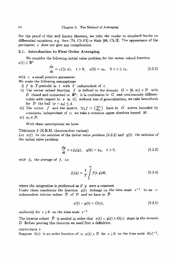
64 Chapter 5. The Method of Averaging
For the proof of this well known theorem, we refer the reader to s tandard books on differential equations, e.g. Ince [74, Ch.III] or Hale [60, Ch.II]. The appearance of the parameter e does not give any complication.
2.1. I n t r o d u c t i o n t o F i r s t O r d e r A v e r a g i n g
We consider the following initial value problem for the vector valued function �9 (t) e R ~
dx dt = e f ( t ' x ) ' t > 0 , x ( 0 ) = x o , 0 < e _ < e o , (5.2.2)
with e a small positive parameter . We make the following assumptions
i) f is T-periodic in t with T independent of e. ii) The vector valued function f is defined in the domain G = [0, c~) • l:) with
D closed and connected in Rn; it is continuous in G and continuously differen- tiable with respect to x in G; without loss of generalization, we take henceforth for l:) the ball I x - x 0 1 _< d.
iii) The vector f and the matr ix v x f = ( ~ . ) have in G norms bounded by
constants, independent of e; we take a common upper absolute bound M. iv) xo E T~.
Wi th these assumptions we have
THEOREM 2 (K.B.M. theorem-first variant) Let x(t) be the solution of the initial value problem (5.2.2) and y(t) the solution of the initial value problem
dy d-t = efo(y), y(0) = x0, t > 0, (5.2.3)
with fo the average of f , i.e.
T 1/ fo(Y) = ~ f ( t , y)dt,
o
(5.2.4)
where the integration is performed as i f y were a constant. Under these conditions the function y(t) belongs on the time scale e -1 to an e- independent interior subset f) of l:) and we have in f)
~ ( t ) - y ( t ) = o ( ~ ) , ( 5 . 2 . 5 )
uniformly for e $ 0 on the time scale e-1.
The interior subset ~ is needed in order tha t x(t) - y(t) + O(e) stays in the domain D. Before proving this theorem we need first a definition.
DEFINITION 1 Suppose 6(e) is an order function of e; ~(t) E 1:) for e $ 0 on the t ime scale 6(e) -1,
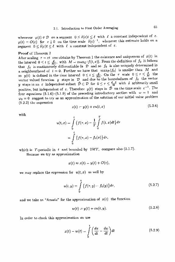
2.1. Introduction to First Order Averaging 65
whenever ~(t) E T) on a segment 0 < 6(e)t < ~ with I a constant independent of e. ~(t) = O(e) for e $ 0 on the time scale 5(e) -1, whenever this estimate holds on a
segment 0 < 5(e)t <_ i with I a constant independent of e.
P r o o f of Theorem 2 After scaling ~- = et one obtains by Theorem 1 the existence and uniqueness of x(t) in the interval 0 < t _~ ~-~, with M = maxG If(t, x)l. From the definition of /0 it follows that I0 is continuously differentiable, ih ~D and so f0 is also uniquely determined in a neighbourhood of t = 0. Further we have that max9 If01 is smaller than M and so y(t) is defined in the time interval 0 _ t < ~--~. On the T scale 0 < T ~ ~ the vector valued function y stays in 2) and due to the boundedness of f0 the vector y stays in an e independent subset 2~ C 2) for 0 _< 7" _< ~ with 6 arbitrarily small
positive, but independent of e. Therefore y(t) stays in ~ on the time scale e -1. The four equations (5.1.6)-(5.1.9) of the preceding introductory section with w - 1 and ~0 -- 0 suggest to try as an approximation of the solution of our initial value problem
(5.2.2) the expression z ( t ) = y( t ) + ~ , ( t , ~) (5.2.6)
with t T / 1/ u(t,x)-- {f(T, X ) - ~ f(t,x)dt}dT
0 0
t
-= / { f (T ,x ) - fo(x)}dT, 0
which is T-periodic in t and bounded by 2MT, compare also (5.1.7). Because we try as approximation
�9 (t) .~ z ( t ) = y( t ) + o (~ ) ,
we may replace the expression for u(t, x) as well by
t
u(t, y) = / {f(z', y) - fo(Y) }dT,
0
(5.2.7)
and we take as "Ansatz" for the approximation of x(t) the function
~(t) = y(t) + ~ ( t , y). (5.2.8)
In order to check this approximation we use
t /(dx x(t) - ~ ( t ) = dt
o
dw ) dt dt
(5.2.9)
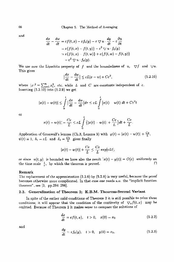
66 Chapter 5. The Method of Averaging
and dx
dt
dy Ou dw = e f ( t x) - e fo (y ) - e V u . -d-[ - e-if[ dt
= e { f ( t , x ) - f ( t , y ) } - e 2 V u . fo(Y)
= e { f ( t , x ) - f ( t , w)} + e { f ( t , w) - f ( t , y ) }
- r V u . f o ( Y ) .
We use now the Lipschitz property of f and the boundedness of u, This gives
dx dw I-d-[ - -~-[ I <- eL[x - w[ + Ce 2,
v f and V u.
(5.2.10)
n 2 etc. while L and C are constants independent of e. where [xl 2 = E i = I x i ,
Inserting (5.2.10)into (5.2.9) we get
t t /dx dw / I x ( t ) - w(t)[ <_ 1-~- - --~-[Idr <_ eL I x ( t ) - w ( t ) l d t + Ce2t
0 0
or t
Ce / Ce Ce Ix(t) - w(t)[ + -~- ___ eL { Ix(t) - w(t)[ + -~-}dt + --ft.
0
Application of Gronwall's lemma (Oh.3, Lemma 3) with qo(t) = Ix(t)- w(t)[ + -~, r - 1 51 -- eL and 52 c~ gives finally
"-- - L - -
I~(t)- ~(t)l + - Cr < Cr exp[eLt] L - L
or since u(t , y) is bounded we have also the result Ix(t)- y(t)]- O(e) uniformly on 1 by which the theorem is proved. [::] the time scale ~,
R e m a r k The replacement of the approximation (5.2.6) by (5.2.8) is very useful, because the proof becomes otherwise more complicated. In that case one needs a.o. the "implicit function theorem", see [3, pp.294-296].
2.2. G e n e r a l i z a t i o n of T h e o r e m 2; K . B . M . T h e o r e m - S e c o n d V a r i a n t
In spite of the rather mild conditions of Theorem 2 it is still possible to relax these conditions; it will appear that the condition of the continuity of v x f ( t , x ) may be omitted. Because of Theorem 2 it makes sense to compare the solutions of
d x d--t = e f (t, x) , t > O, x(O) = xo (5.2.2)
and
dy _ e fo ( y ) , t > O, y(O) xo (5.2.3) dt
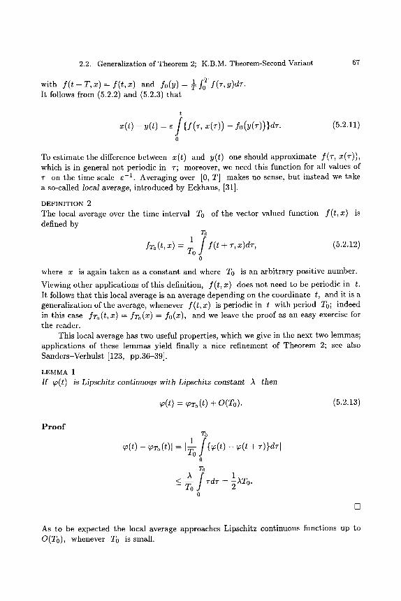
2.2. Generalization of Theorem 2; K.B.M. Theorem-Second Variant
with f (t + T, x) = f (t, x) and fo(Y) = -~ fo T f (~-, y)dT. It follows from (5.2.2) and (5.2.3) that
67
t
~(t) - y(t) = ~ f {f(~, ~(~)) - f0 (y (~ ) )}a~ . 0
(5.2.11)
To estimate the difference between x(t) and y(t) one should approximate f(T, X(T)), which is in general not periodic in T; moreover, we need this function for all values of T on the time scale e-1. Averaging over [0, T] makes no sense, but instead we take a so-called local average, introduced by Eckhaus, [31].
D E F I N I T I O N 2
The local average over the time interval To of the vector valued function f ( t , x) is defined by
To 1 /
fT~ = Too f ( t + T,x)dT, (5.2.12)
0
where x is again taken as a constant and where To is an arbitrary positive number.
Viewing other applications of this definition, f( t , x) does not need to be periodic in t. It follows that this local average is an average depending on the coordinate t, and it is a generalization of the average, whenever f ( t , x ) is periodic in t with period To; indeed in this case fTo (t, x) = fTo (x) = f0(x), and we leave the proof as an easy exercise for the reader.
This local average has two useful properties, which we give in the next two lemmas; applications of these lemmas yield finally a nice refinement of Theorem 2; see also Sanders-Verhulst [123, pp.36-39].
L E M M A 1
I f 99(t) is Lipschitz continuous with Lipschitz constant A then
~(t) = ~ o (t) + O(To). (5.2.13)
P r o o f To 1/
I~(t) - ~To(t) l - - IT0 {~(t) -- 9o(t + T)}dTI 0
To 1
< TdT = ATo - T o -~
o
As to be expected the local average approaches Lipschitz continuous functions up to O(T0), whenever To is small.
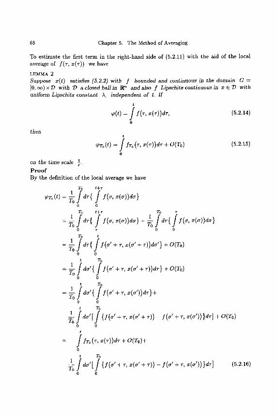
68 Chapter 5. The Method of Averaging
To estimate the first term in the right-hand side of (5.2.11) with the aid of the local average of f(T, X(T)) we have
L E M M A 2 Suppose x(t) satisfies (5.2.2) with f bounded and continuous in the domain G = [0, oo) x/9 with 7) a closed ball in 1R n and also f Lipschitz continuous in x E 1) with uniform Lipschitz constant A, independent of t. I f
t
~(t) = / S(~, ~(~))~, (5.2.14)
0
then t
~,% (t) = i f% (% ~(r))a~- + O(To) 0
the time scale }. o n
P r o o f By the definition of the local average we have
To t + r 1
~%(')- ~o f~': i :(" ~('))~') 0 o
To t+r To ~-
i I ' I i To 0 "r 0 0
To t
: '-~o i ~ i,(~ + ~, ~(~ ~>>~~ + o(~o> 0 0
t To
: '-~o I~~ I , (~ +-, ~(~ +,>>~,} + o(~o> o 0
t To
: '-,o i~:'~ i , ( ~ =(~ 0 0
t To
1 i i Too da'[ { f ( a ' + r, x(a' + T)) -- f ( a ' + T, x(a'))}dT] + O(To) o o
t
= i fTo (% X(v))aT + O(To)+ 0
t To
d~'[ {s(<,' + -, ~(~' + -)) - s(~' + - , ~(~'))}d, ] o o
(5.2.15)
(5.2.16)
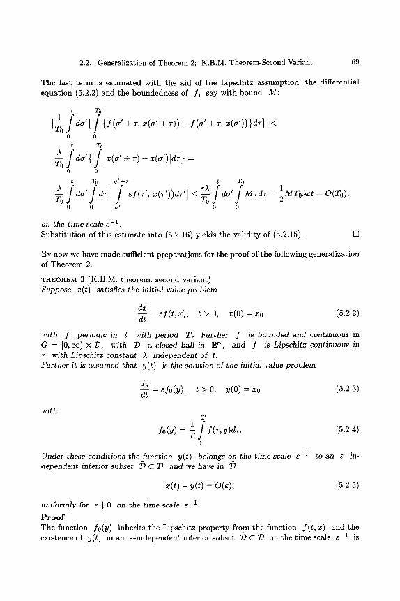
2.2. Generalization of Theorem 2; K.B.M. Theorem-Second Variant 69
The last term is est imated with the aid of the Lipschitz assumption, the differential equation (5.2.2) and the boundedness of f , say with bound M:
t To 1/ / 0 0
t To A .of
0 0
t To a'+~" t To
f f f eAff 1 A da' dT[ e f ( T t ' X ( T t ) ) d T t [ < TOO da' M T d T = ~ M T o A e t = O(To) O " - - '
0 0 a ~ 0 0
on the time scale e -1. Substi tution of this estimate into (5.2.16) yields the validity of (5.2.15).
By now we have made sufficient preparations for the proof of the following generalization of Theorem 2.
T H E O R E M 3 (K.B.M. theorem, second variant) Suppose x(t) satisfies the initial value problem
d x dt = 6 f ( t , x ) , t > O, x(O) = Xo (5.2.2)
with f periodic in t with period T. Further f is bounded and continuous in G = [0, cx~) x 79, with 79 a closed ball in R '~, and f is Lipschitz continuous in x with Lipschitz constant A independent of t. Further it is assumed that y(t) is the solution of the initial value problem
dy = cfo(y), t > O, y(O) = xo (5.2.3)
dt
with T 1/
fo(Y) = ~ f(T, y)dT.
0
(5.2.4)
Under these conditions the function y(t) belongs on the t ime scale e -1 to an e in- dependent interior subset f) C 79 and we have in f)
�9 ( t ) - y ( t ) - o ( ~ ) , ( 5 . 2 . 5 )
uniformly for e $ 0 on the time scale e-1.
P r o o f The function fo(Y) inherits the Lipschitz property from the function f ( t , x ) and the existence of y(t) in an e-independent interior subset ~ C 79 on the time scale e -1 is
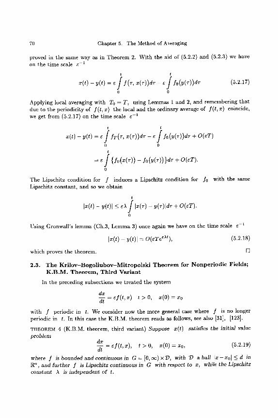
7O Chapter 5. The Method of Averaging
proved in the same way as in Theorem 2. Wi th the aid of (5.2.2) and (5.2.3) we have on the t ime scale e -1
t t
x(t) - y(t) - r / f (T, X(T))dT -- e / fo(y(T))dT (5.2.17)
0 0
Applying local averaging with To - T, using Lemmas 1 and 2, and remember ing tha t due to the periodicity of f ( t , x ) the local and the ordinary average of f ( t , x ) coincide, we get from (5.2.17) on the t ime scale e -1
t t
f - : / f o + 0 0
t
= e / { fo (x(r)) - fo (y(r)) }dr + O(eT).
o
The Lipschitz condition for f induces a Lipschitz condition for f0 with the same Lipschitz constant , and so we obtain
t
Ix(t) - y(t)[ < EA / I x ( T ) - y(T)ldT + O(eT). 0
Using Gronwall 's l emma (Ch.3, L e m m a 3) once again we have on the t ime scale e -1
I x ( t ) - y ( t ) l - O(eTe~t ) , (5.2.18)
which proves the theorem.
2.3. The Kri lov-Bogol iubov-Mitropolski Theorem for Nonperiodic Fields; K.B.M. Theorem, Third Variant
In the preceding subsections we t rea ted the system
dx d---t = e f (t' x) t > 0 , x ( 0 ) = x 0
with f periodic in t. We consider now the more general case where f is no longer periodic in t. In this case the K.B.M. theorem reads as follows, see also [31], [123].
THEOREM 4 (K.B.M. theorem, third variant) Suppose x(t) satisfies the initial value problem
d_ff = e f ( t x) t > 0, x(0) = x0, (5.2.19) dt ' '
where f is bounded and continuous in G = [0, oo) x T), with 1) a ball I x - x 0 l ~_ d in ]R ~, and further f is Lipschitz continuous in G with respect to x, while the Lipschitz constant A is independent of t.
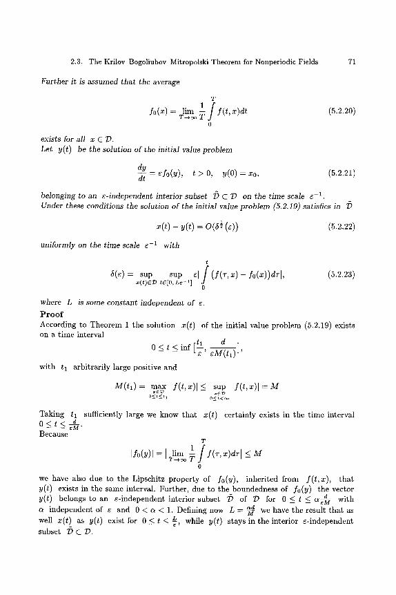
2.3. The Krilov-Bogoliubov-Mitropolski Theorem for Nonperiodic Fields 71
Further it is assumed that the average
T
f o ( x ) = lim 1 f T - ~ T f (t, x)dt 0
(5.2.20)
exists for all x C 79. Let y(t) be the solution of the initial value problem
dy d---[ = efo(y), t > O, y(O) = xo, (5.2.21)
belonging to an e-independent interior subset f) C 79 on the time scale e - 1 .
Under these conditions the solution of the initial value problem (5.2.19) satisfies in f)
- y ( t ) = (5.2.22)
uniformly on the time scale e -1 with
t
5(e) = sup sup ~1 f fo(x))dTI, (5.2.23) x ( t ) E T ) tE[O,Lr -1]
0
where L is some constant independent of e.
P r o o f According to Theorem 1 the solution x(t) of the initial value problem (5.2.19) exists on a time interval
0 _< t _< inf [t2 d
e ' eM(t l ) ]'
with tl arbitrarily large positive and
M( t l ) : max I f ( t ,x) l <_ sup If(t,x)l : M =ET~ =E~D
O < t < t l O_<t<oo
Taking tl sufficiently large we know that x(t) certainly exists in the time interval 0 ( t ( d
w e M "
Because T
I f o ( v ) l - [ lim 1 f T - ~ T f (T' x)dTI <- M 0
we have also due to the Lipschitz property of fo(Y), inherited from f ( t , x ) , that y(t) exists in the same interval. Further, due to the boundedness of fo(Y) the vector y(t) belongs to an e-independent interior subset ~ of 79 for 0 < t < c~?-4MM with a independent of e and 0 < a < 1. Defining now L - -~ we have the result that as
L while (t) stays in the interior e-independent well x(t) as y(t) exist for 0 _ < t < - g , y subset 7} C 79.
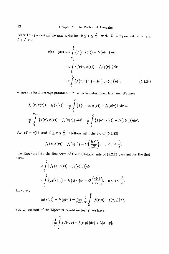
72 Chapter 5. The Method of Averaging
After this precaution we may write for 0 < t _ ~, with L independent of ~ and O < L < L
t
�9 (t) - y(t) = ~ f { s (~ , ~(~)) - fo ( y ( ~ ) ) } ~ 0
t
= ~ f {s~(~, ~(,)1 - So(y(,))}d, 0
t
+ ~ f {s(,, ~(,)) - s~(,, ~(,))}e,, o
where the local average parameter T is to be determined later on. We have
(5,2.24)
T 1/ 0
T + r 1/ 1] {s(~', ~(,)) - s 0 ( ~ ( , ) ) } e ~ , - ~ {s(~' , ~(,)) - s0(~(~))}e~,.
0 0
For ~ T - o(1) and 0 < T < L_-~ it follows with the aid of (5.2.23)
Inserting this into the first term of the right-hand side of (5.2.24), we get for the first term
t
f {s~(. , ~(.)) - s0(y( . ) )}e . = 0
t
~o
c 0
However, T
fo (X(T)) -- fO (y(T)) -- lim 1 / ~-~oo ~ {s(r ,~)- SO-,y)}dT, 0
and on account of the Lipschitz condition for f we have
T
if I~ {s(r,=)- so-,y)}~rl < AIx-y l , o
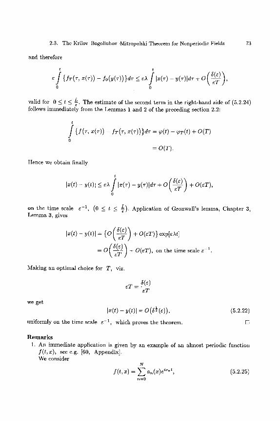
2.3. The Krilov-Bogoliubov-Mitropolski Theorem for Nonperiodic Fields 73
and therefore
t t
0 0
valid for 0 < t _ L__-. The estimate of the second term in the right-hand side of (5.2.24) follows immediately from the Lemmas 1 and 2 of the preceding section 2.2'
t
/ { s (~ , ~(~)) - s~(~, ~(~)) }d~ = ~(t) - ~ ( t ) + O(T) 0
= O(T).
Hence we obtain finally
t
0
, s on the time scale r (0 _ t _~ -j). Application of Gronwall's lemma, Chapter 3, Lemma 3, gives
]x ( t ) - y(t)[ = { 0 ( 5 r 1 6 2
= O(~T) )+O(r on the time scale r
Making an optimal choice for T, viz.
eT = 5(r cT
we get
Ix(t)- y(t)l- 0(5�89 (~)), uniformly on the time scale r which proves the theorem.
(5.2.22)
D
R e m a r k s
1. An immediate application is given by an example of an almost periodic function f(t,x), see e.g. [60, Appendix]~ We consider
N
f(t ,x) = E an(x)eiVnt' (5.2.25) n--O
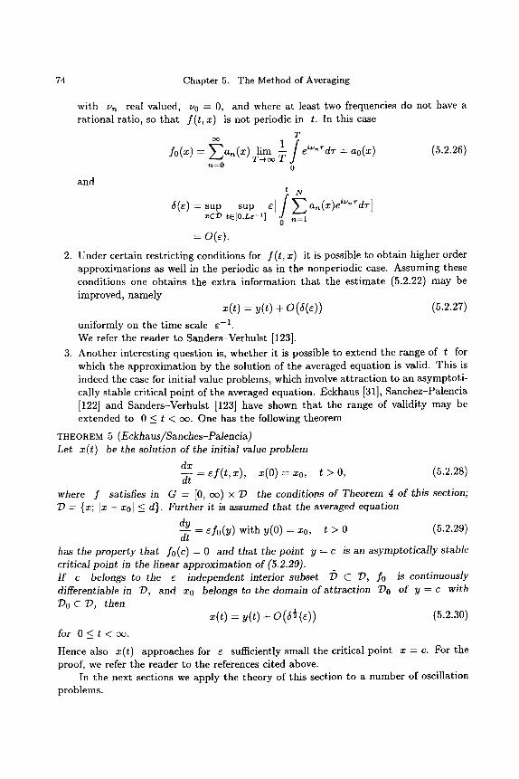
74 Chapter 5. The Method of Averaging
with un real valued, v0 = 0, and where at least two frequencies do not have a rat ional ratio, so tha t f ( t , x) is not periodic in t. In this case
T o o
fo(X) = E an(x) T-.oolim ~1 / ei~n~d T _ ao(x) (5.2.26) n = O 0
and
5(e ) = sup sup e I a.(x)eW"~dT] xED tE[O,Le -1] 0 n=l
= o ( ~ ) .
2. Under certain restricting conditions for f ( t , x ) it is possible to obtain higher order approximations as well in the periodic as in the nonperiodic case. Assuming these conditions one obtains the extra information tha t the est imate (5.2.22) may be improved, namely
x(t) = y(t) + O(5(e)) (5.2.27)
uniformly on the t ime scale e -1. We refer the reader to Sanders-Verhulst [123].
3. Another interesting question is, whether it is possible to extend the range of t for which the approximat ion by the solution of the averaged equation is valid. This is indeed the case for initial value problems, which involve a t t rac t ion to an asymptoti- cally stable critical point of the averaged equation. Eckhaus [31], Sanchez-Palencia [122] and Sanders-Verhulst [123] have shown tha t the range of validity may be extended to 0 _< t < o0. One has the following theorem
THEOREM 5 (Eckhaus//Sanches-PMencia) Let x(t) be the solution of the initial value problem
dx = ~ f ( t , ~), ~ ( 0 ) = ~0, t > 0, ( 5 . 2 . 2 s )
dt where f satisfies in G = [0, oo) x D the conditions of Theorem 4 of this section; /9 = {x; x - Xo[ _< d}. Further it is assumed that the averaged equation
dy dt = efo(y) with y(O) = xo, t > 0 (5.2.29)
has the property that fo(c) = 0 and that the point y = c is an asymptotically stable critical point in the linear approximation of (5.2.29). I f c belongs to the ~ independent interior subset Z) C 7), fo is continuously differentiable in l), and xo belongs to the domain of attraction 7)o of y - c with 7)o C I), then
x(t) = y(t) + 0(5�89 (e)) (5.2.30)
for O < t < c~.
Hence also x(t) approaches for e sufficiently small the critical point x = c. For the proof, we refer the reader to the references cited above.
In the next sections we apply the theory of this section to a number of oscillation problems.
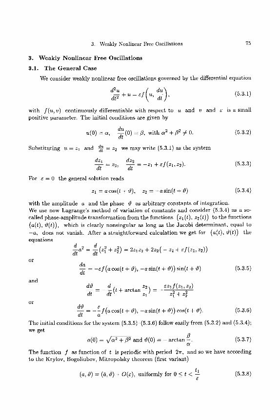
3. Weakly Nonlinear Free Oscillations 75
3. W e a k l y N o n l i n e a r F r ee Osc i l l a t i ons
3.1. T h e G e n e r a l C a s e
We consider weakly nonlinear free oscillations governed by the differential equation
d2u ( d u ) (5.3.1) d t---~ -t- u = ~ f u , - - ~ ,
with f ( u , v ) continuously differentiable with respect to u and v and e is a small positive parameter. The initial conditions are given by
du u(0) = a, -~(0) - / 3 , with C~ 2 -~-/~2 r 0. (5.3.2)
Substi tuting u - zl and du -~ = z2 we may write (5.3.1) as the system
dzl dz2 _ dt = 22, dt - - z l + ~ f ( z l , z2). (5.3.3)
For r = 0 the general solution reads
Zl - - a cos(t + 0), z2 = - a s i n ( t + 0) (5.3.4)
with the amplitude a and the phase 0 as arbitrary constants of integration. We use now Lagrange's method of variation of constants and consider (5.3.4) as a so- called phase-amplitude transformation from the functions (zl (t), z2(t)) to the functions (a(t), O(t)), which is clearly nonsingular as long as the Jacobi determinant, equal to - a , does not vanish. After a straightforward calculation we get for (a(t) , O(t)) the equations
d a 2 d d-t - - d-t (z12 -~- z22) - - 2ZlZ2 "~- 2 z 2 ( - - z l -~- ~/(z~, z2))
or
and
or
da = - r + O ) , - a sin(t + 0) )s in( t + 0) (5.3.5)
dt
~11) ~zlf(zl, z2) dO _ d (t + arctan - - dt - dt z 2 + z 2
dO e = - - f ( a c o s ( t + 0), - a sin(t + O)) cos(t + 0). (5.3.6)
dt a
The initial conditions for the system (5.3.5)-(5.3.6) follow easily from (5.3.2) and (5.3.4); we get
a(0) -- V/a 2 +/32 and 0(0) - - arctan -~. (5.3.7) a
The function f as function of t is periodic with period 2~, and so we have according to the Krylov, Bogoliubov, Mitropolsky theorem (first variant)
tl (a, 0) - (5, ~ ) + O(E), uniformly for 0 _ t < -- (5.3.8)
c
76 Chapter 5. The Method of Averaging
with tl some constant independent of e and with (a, 0) satisfying the averaged equations
21r
da r f d--t- = 27r j f (~cos( t + tg), -~ s in ( t + tg)) sin(t + ~)dt
0
and
dr9 dt
271-
a27r f (a cos(t + tg), - a sin(t + tg)) cos(t + ~)dt 0
o r 271"
da r f d-t - = 21r f (a cos ~0, - a sin ~o) sin ~od~o (5.3.9)
0
and 211"
dr9 e f d-t = a2 r f ( a cos ~o, - a sin ~) cos ~ad~a, (5.3.10)
0
with a(0) = V/a 2 +/32 and zg(0) - - a r c t a n / 3 . (5.3.11)
The solution of this autonomous system gives a first order approximation for (a(t), O(t)) and hence also for u(t) = a(t)cos (t + ~(t)) and the approximation is uniformly valid for 0 _~ t < tl/r with tl some number independent of e.
For practical applications it is useful to have an estimate for the value of tl. Suppose that the greatest of the upper bounds of ]f{acos(t + ~), - a s i n ( t + zg)} I and I ~ f { a c ~ in the domain (D) 0 < t < c ~ , 0_~ l a -v / c~ 2+/32 I _ d , 0_~ I z g + a r c t a n ~ l < c ~ is Md (in case fT(=0 for a = 0 , we
should take d < V/c~ 2 +/32 ), then the solution of the initial value problem (5.3.5), (5.3.6), (5.3.7) exists for any positive value of e and for
d 0 < t <
- - ~ M d "
This follows from a modification of the formulation of the existence Theorem 1 (see e.g. [74], p.71); the value of t* appearing in Theorem 1 does not play any role since t* = cx:). Because the solution (~, zg) of the averaged equation should stay in an interior domain 7) C D the time interval [0, ~Md] should be shortened to [0 d-~ , 7-M--~] with ~ arbitrarily small positive, but independent of e. Hence the value of tl is ( d - ~)/Md. We remark that in general Md increases with d and so the value of tl may decrease, whenever d increases. Further it should be noted that in case Md is uniformly bounded by M for all value of d, then t l - - ~ with d arbitrarily large. This may happen, for instance, in oscillation problems with damping, see subsection 3.4.
3.3. The Perihelium Precession 77
3.2. T h e D u r i n g E q u a t i o n
We consider the initial value problem (4.2.1)-(4.2.2) of Chapter 4:
d2u dt 2 ~ u + e U 3 = 0 (5.3.12)
d~t with the initial conditions u(0) = a =/= 0, -du = 0. Applying the K.B.M. theorem and the results of the last subsection we get
t l u( t ) = a(t)cos (t + tg(t)) + O(e), uniformly for 0 < t < --
with (a, 0) satisfying the initial value problem
27I" da e / ~ 3 d--t- = ~ COS3 (p sin cpd~, a(O) = a
0
2~"
dO _ e J a3 COS4 ~dcp, 0(0) = O. -dt - 2~ra
0
It follows immediately that
a(t) -- a and ~(t) = 3za2t ,
and therefore 3
u( t ) = c~cos{(1 + gec~2)t} + O(e) (5.3.13)
uniformly for 0 < t < t~ with tl some constant. This result is in agreement with the formula (4.2.18) of Chapter 4.
3.3. T h e P e r i h e l i u m P r e c e s s i o n
The trajectory of a planet around the sun is according to section (4.2.1) given by a solution of the differential equation
d2u
d~ 2 + u -- a + eu 2 (4.2.19)
where G M m ~ 3 G M m
u = - a = and e = << 1. , h 2 r c 2 r
(r, 0) are the polar coordinates of the center of the planet with respect to the center of the sun and ~ is a characteristic length. As to the other physical constants one is referred to Chapter 3, section 3.2. As initial conditions, we choose again
du u(o) = ~, -~ = ~.
78 Chapter 5. The Method of Averaging
We put u = a + av and v satisfies the initial value problem
d 2 v
dO 2 ~ - v = c a ( l + v ) 2, v (O)= o[. - a dv
dO (0) = a
The K.B.M. theorem yields again
v(o) = A(o)cos (o + ~(o)) + o(~),
uniformly for 0 < 0 < ~-~ with 01 some positive constant while A and (~ satisfy the differential equations
2~" dA 1 / dO = -ea-~-~ (1 + A c o s ~ ) 2 s i n ~ d ~ - 0
0
and
d ~ ) _
d O -
So it follows from (5.3.11)
291"
eaA= 21rl J ( 1 + Acos ~) 2 cos ~d~ = -~a .
0
and
So we obtain
ft. = constant = _1 V/(C ~ _ a) 2 + ~2 a
~ ) . = - ~ a 0 - arctan (c~ - a
o r
)} + o(~) 1 V/-ic ~ _ a) 2 +/32 cos { (1 - ~a)0 - arctan ( a _ a v ( 0 ) - a
u(O) : a + V / ia - a) 2 + ~2 cos { (1 - ca)O - arctan ( a fl ) } + 0(r - a (5.3.14)
uniformly for 0 < 0 < ~-~ with 01 some positive number, independent of ~. This result is in agreement with formula (4.2.29) of Chapter 4.
3.4. T h e L i n e a r O s c i l l a t o r w i t h S m a l l Damping
We consider a linear oscillator with small damping, represented by the initial value problem
d2u du dt--- ~ + 2~-~- + u = O, t > O, (5.3.15)
with the initial conditions d u
u(O) -- O, -~/-(0) = 1. (5.3.16)
3.5. The Free Van der Pol Equation 79
I l lus t ra t ing the m e t h o d we apply the phase -ampl i tude t r a n s f o r m a t i o n and we get for the ampl i t ude and the phase the init ial value problems
da = r cos 2(t + tO) - 1}, dO dt dt
= - e s i n 2(t + tO), (5.3.17)
wi th
Averaging yields
71" a ( 0 ) = 1 , tO(0)= 2
d~z dtO - ~r dt -e~z, --~ 0; a(0) 1, tO(0)= 2
Hence 71"
a( t ) = e - a + O ( e ) , tO(t) = - - ~ + O ( e ) ,
uni formly valid for 0 < t < ~ wi th t l an a r b i t r a r i l y large posi t ive number , i ndependen t of e. The la t t e r follows from the fact t h a t the r igh t -hand sides of (5.3.17) are uni formly bounded for all values of t, a and tO wi th a > 0 , ( da < 0 and so a( t ) < 1 ) see subsect ion 3.1. Hence
du -~t u ( t ) - e -~ t sin t + O(~) and - ~ = e cos t + O(e) , (5.3.18)
uni formly valid for all values of t, 0 _< t < oo.
3 .5. T h e F r e e V a n d e r P o l E q u a t i o n
This equa t ion reads
d2x d x (5.3.19) + x -- e(1 - x 2 ) - ~ -. dt---g
The general so lut ion may be a p p r o x i m a t e d as
tl x ( t ) -- ~ ( t ) c o s (t + 0( t ) ) + O(e) uni formly for 0 < t <
wi th
dd
dt
27F
2rr (1 - cos 2 qo)sin 2 qodqo = T 1 - -~- ,
0
d~
dt
271"
. / ~2 21r (1 - cos 2 ~o) sin ~o cos ~odqo - O.
0
We leave it to the reader to show t h a t one m a y take t l a rb i t ra r i ly large. After an e l emen ta ry ca lcula t ion we get
~ 2 .__
1 - A e - e t ' = cons tan t = ~(0) "= too,
80 Chapter 5. The Method of Averaging
where A and t~0 are de te rmined by initial conditions. Hence
2 x( t) = cos(t + ~o) + 0 (~ ) , (5.3.20)
V/1 Ae-~t
uniformly for 0 < t < t_x with t l an a rb i t r a ry positive number , independent of ~. E
In case x ( 0 ) = c ~ > 0 and dx -aT(0) = 0 we have according to (5.3.7) and (5.3.11)
V/1 - A = c~ and Oo = 0
o r
4 A = 1 c~ ~ and ~ 0 - 0. (5.3.21)
In contras t to the foregoing examples , it is not the phase tha t changes slowly wi th t ime, but it is now the ampl i tude; this is, of course, due to the damping t e rm e(1 - x 2) dx ~-.
The ampl i tude increases for c~ < 2, and decreases for c~ > 2; for c ~ - 2 the mot ion differs from a periodic mot ion only in a t e rm O(e) as long as 0 < t <
4. W e a k l y F o r c e d Nonl inear Osci l lat ions
4.1. T h e Case w i t h o u t D a m p i n g
We consider the nonhomogeneous Duffing equat ion
d2u
dt 2 4- u 4- ~u 3 - eA coswt, 0 < ~ < < 1 , A > 0 , (5.4.1)
wi th the initial condit ions du
u(O) = ~, ~ ( o ) = o.
The frequency w of the driving force is nearly equal to the frequency of the oscillation in case ~ = 0; w is defined by w2 = 1 4- ~# wi th # some posit ive or negative number independent of ~. We want to invest igate the influence of the forcing t e r m on the mot ion as described in section 3.2 of this chapter . P u t t i n g again Zl = u and z2 = -~ the equat ion (5.4.1) is equivalent wi th the sys tem
dzl dz2 - z2, - - Z l - cz 3 4- EA cos wt. (5.4.2) _
dt dt
Ins tead of the nonsingular t r ans fo rmat ion (zl , z2) -4 (a, v~) given by
Zl ---- a cos(t 4- tg), z2 -- - a sin(t 4 i 0), (5.3.4)
we use now the nonsingular t r ans fo rmat ion
zl -- a cos(wt + v~), z2 = - a w sin(wt + ~), (5.4.3)
4.1. The Case without Damping 81
with a = a(t) , to=to( t ) a n d a ( 0 ) = c ~ a n d t o ( 0 ) = 0 .
We insert this transformation into (5.4.2), and we get for a2(t) the equation
(5.4.4)
d a 2 _ d z ~ : 2 z l z 2 ( 1 - 1 2~z2 d-~ ~ (212 + ~ . , ~ ) - ~ (z~ - A cos ~t)
_ _ _ a 4
= e [ #a2 sin 2(cot + to) + - - s i n 2(cot + to)cos 2 (cot + to) co co
_ 2a____AA sin(cot + to)cos cot]. co
After an elementary calculation we get finally for the amplitude a(t) the equation
da a a 2 a 3 dt =e[~co (-~- - #)sin2(cot + to)+ ~--co sinn(cot + to)
A - -- sin(cot + to)cos cot] =
co a a 2 a 3
e [~co (-~- - #) sin2(cot + to)+ ~--co sin 4(cot + to)
A A sin(2cot + to) - 2---w sin to].
2co (5.4.5)
Since wt + to = - arctan ~ we get for to(t) the differential equation wz1
dto d z 2 w z 2 f z l ' d Z - ~ - - z 2 d z l ~ d---t- = - w ~ a r c t a n - = - w - _ ~ dt
~z~ ~ 1 + z i zf CO
: - --CO - - CO2Z 2 -+- Z2 { Z l ( - - Z x - - ~ Z 3 -~- cA cos cot) - z 2 }
- ~ ( - ~ z ~ + z ~ - A z ~ c o s ~ t } - ~2z~ + z]
= ~ { - , z ~ + z 4 - Az~ cos~t}. a 2 co
We have a 2 z 2 = a 2 cos2(wt + to) = --~-{1 + cos 2(wt + to)}
and a 4
z 4 = -~- { 3 + 4 cos 2 (wt + to) + cos 4 (wt + to) }
and substitution gives for to(t) the differential equation
dto dt a2w
a2w
a 4
~a~ 2(~t + ~)} + -g ~ [ - --f- {1 + c o s { 3 + 4 cos 2(wt + to) + cos 4(wt + to)}
- Aa cos(wt + to)cos wt] - - # a 2 a 4
~ [ 2 {1 + c o s 2 ( w t + t o ) } + - ~ { 3 + 4 c o s 2 ( w t + ~ ) + c o s 4 ( w t + t o ) }
Aa Aa 2 cos(2wt + to) 2 cos tO]. (5.4.6)
82 Chapter 5. The Method of Averaging
The right-hand sides of (5.4.5) and (5.4.6) are periodic in t with period 2~ -~-, and so by using Theorem 3 of section 2.2 of this chapter the functions a( t ) and 0(t) may be approximated uniformly in 0 < t < k by the solutions of the equations
d~ w f d~ = ~ (
0
_ __A s in0)d t = e A sin0, (5.4.7) 2w 2w
and
dt~ _ r w f a 2 3a4 _ ~Aa ~ ) d t d t - a 2 w 2 r ( - t t - ~ - + ~ 2 cos
0
--r 3 r 2 c A -
= - t cos O, 2w 8 w 2gw
(5.4.s)
with the initial conditions a(0) - a, t~(0) = 0. (5.4.9)
The constant tl is again some positive number, independent of ~. The critical point of the system (5.4.7)-(5.4.8) is given by (ac, 0) with
3 _ 3 ~a~ - a ~ # - A - 0.
Therefore, in case u(0) = a satisfies the condition
3a3 a # A 0, 4
or with w 2 - 1 + r
3 A (5.4.10) w 2 = 1 + -~ea 2 - e--,a
the solution of the nonhomogeneous Duffing equation (5.4.1) with u(0) - a and du d-y(0) = 0 may be approximated as
u ( t ) = a cos wt + O(e), (5.4.11)
uniformly for 0 < t < ~ . We encounter here a remarkable phenomenon: for r = 0 the solution of the initial value problem (5.4.1) reads
u ( t ) = a cos t,
while a small perturbation, resulting into (5.4.1), gives an approximate solution
t l u( t ) = a c o s w t , 0 ~ t < L - - ,
E
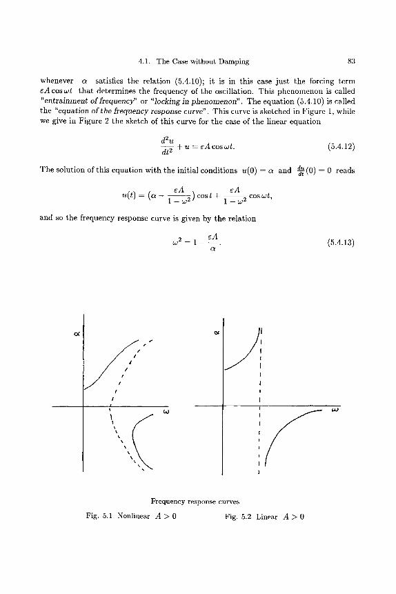
4.1. The Case without Damping 83
whenever a satisfies the relation (5.4.10); it is in this case just the forcing te rm r cos wt tha t determines the frequency of the oscillation. This phenomenon is called "entrainment of frequency" or "locking in phenomenon". The equat ion (5.4.10) is called the "equation of the frequency response curve". This curve is sketched in Figure 1, while we give in Figure 2 the sketch of this curve for the case of the linear equat ion
d2u + u = r cos wt. (5.4.12)
dt 2
The solution of this equat ion with the initial conditions u(0) - a and du -3)- (0) -- 0 reads
CA CA u( t )= (a 1 - w 2 ) c ~ 1 w2COSWt,
and so the frequency response curve is given by the relation
w 2 _ l ~A
(5.4.13)
s s
s'
t
t
| I
!
I I I
I ! f I
I
I t i
I
I !
Frequency response curves
Fig. 5.1 Nonlinear A > 0 Fig. 5.2 Linear A > 0
84 Chapter 5. The Method of Averaging
4 . 2 . T h e C a s e w i t h D a m p i n g
The results of the last subsection are so intriguing, that it is worthwhile to consider also the case with a little bit of damping. So we study the differential equation
d2u du + eS-=. + u + eu 3 = eA coswt,
dt--- V dt t > 0, (5.4.14)
with 5 positive and independent of e, 0 < e << 1, w 2 = l + e # and A > 0. We introduce again the transformations (u, -+ (Zl, Z2) ~ (a, @)"
u = Zl -- a cos(wt + O)
du = z2 = - a w sin(wt + @),
dt (5.4.3)
and we repeat the procedure of Section 4.1. The results are:
da [ a a 2 5a {cos 2(wt + ~) _ l } d--t- = e ~ww (-2- - ~u) sin 2(wt + t~) + -~-
a 3 A sin(2wt + @) A sin v~] + ~ww sin 4(wt + tg) - ~ - 2---w (5.4.15)
and
dO e dt a2w
- - # a a 4
- - 2 { 1 + cos 2(wt + 0) } + -~- { 3 + 4 cos 2(wt + O) + cos 4(wt + O) }
a2~w sin 2(wt + tg) Aa cos(2wt + @) Aa ] . . . . . . cos@ (5.4.16)
2 2 2 J
The solution of this set of equations with certain initial conditions is approximated up to order O(e), uniformly in [0, ~ ) with tl arbitrary and positive by the solution of the set
= - e z w s i n t ~ +
dr9 [ # 3 a 2 A
dt - e 2w 8 w 2~tw
(5.4.17)
- - cos tg) (5.4.18)
where ~ and t~ satisfy the same initial conditions as the functions a and 0. The critical point of the system (5.4.17)-(5.4.18) is given by
A 5a~ + - - s in ~ = 0
w
and 3_2 A
- - - cos ~ = #, ac ac
(5.4.19)
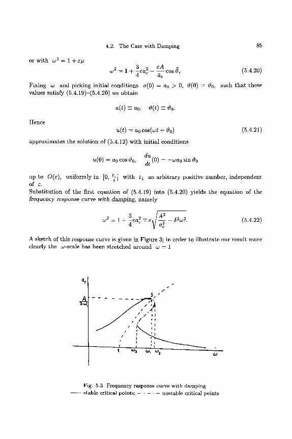
4.2. The Case with Damping 85
or with w 2 = 1 + 6 # 36~ ~ 6A
-- - J cos0c (5.4.20) w 2 1 + ~ a,,:
Fixing w and picking initial conditions a(0) = ao > 0, 0(0) = 00, such tha t these values satisfy (5 .4 .19)-(5.4.20)we obta in
a(t) -= a0, tg(t) = ~o.
Hence
u(t) = ao cos(wt + ~)0)
approximates the solution of (5.4.12) with initial conditions
(5.4.21)
d u
u(0) -- ao cos ~o, -~- (0) -- - w a o sin ~o
up to O(6), uniformly in [0, ~] with t l an arb i t ra ry positive number , independent of 6. Subs t i tu t ion of the first equat ion of (5.4.19) into (5.4.20) yields the equat ion of the frequency response curve with damping, namely
3ca2 T 6 - 52w 2. w 2 = 1 + ~ (5.4.22)
A sketch of this response curve is given in Figure 3; in order to i l lustrate our result more clearly the w-scale has been stretched around w - 1
f
. ~ t t . , . . . . , . . . . . . . . . . �9
/ . ' I " , , / o i J , ' , ( :,
~ I r ~ ', ! . r ~ ' I t a
! I ! I
t O
Fig. 5.3 Frequency response curve with damping stable critical points; . . . . . unstable critical points
86 Chapter 5. The Method of Averaging
3 2 The part of the curve left to the hyperbola ~O 2 : 1 § ~r corresponds with the - sign and the part to the right with the + sign in (5.4.22). For a value of w with w2 < w < w3 there exist three values of a~, and so we have in principle three solutions (5.4.21) with entrainment of frequency and the question arises, which branch might represent a stable solution. To answer this question we return to the averaged equations (5.4.17)-(5.4.18) and make a stability analysis.
at = - r ~ww sin ~ + . - F ( a , ~, w)
d~ ( # 3a2 A ) d--t = - r t cos z~ = 2w 8 w 2~w
w 2 - 1 - 3ea2 + ~--cos t~ := G(a, t~,w) 2w 4 a
(5.4.23)
(5.4.24)
For the investigation of the stability of the equilibrium points lying on the frequency response curve, it is sufficient to study the linear approximation of (5.4.23)-(5.4.24) in the neighbourhood of these equilibrium points. According to the Poincar~-Lyapunov theorem (see e.g. [123], or [60, p.190]) an equi- librium point is asymptotically stable, whenever the eigenvalues of the matrix
M
OF O_..~F ) oa o~ OG OG -0--d ~ a=ac, ~=~
have negative real part and the equilibrium point is unstable, whenever at least one eigenvalue has positive real part; ( f i ( t ) - ac and ~ ( t ) - tgc decay exponentially to zero, whenever the real parts of the eigenvalues are negative). It is now easily derived that a sufficient and necessary condition for the stability is given by
OF OG) < 0 (5.4.25)
and
We have
and
det M OF OG OF - = > 0 (5.4.26) 0a 0~ 0~ ~a a . . . . ~=~c
OF 5 OF A 0a (a~, ~ ) = - ~ , b-~ (a~' ~ ) = - ~ 2 ~ c o s ~
OG 3 A cos0~
OG A sin 0~
o~ (a~, ~ ) = ~-2~ a~ -- - ~ '
5. A Linear Oscillator with Increasing Damping 87
see (5.4.19). The first condition (5.4.25) is trivially satisfied, because we assumed ~ and 5 positive and there remains only to establish the sign of the determinant of M along the response curve given by F(a~, ~ , 02) - O, G(ac, 0~, 02) = 0. Differentiating with respect to 02 we get along this curve
OF OF da~ OF d~)~ 002 = Oa------~ d----w + i ) ~ d w ' OG OG da~ OG d~c 002 cOa~ dw 00~ dw '
elimination of ~ yields and dw
_ _ ( o a o F da~ . det M - d02 \ 002 0 ~ 002 00~ "
Hence the sign of det M is determined by the sign of
d02 002 00~ 002 ~
dac [e A A d02 ~ 2 0 2 c o s ~ - ( e sinO~)(e
A sin ~)~ ) }
202 ac '
which by (5.4.19) and (5.4.20)equals
1 dac 3 2 202 d02 {ac(1 + 4 e a c - 022)_ le252ac } (5.4.27)
Neglecting the term of O(e 2) we get for positive values of ac and 02 a positive determinant M and hence stability, whenever
3 2 022 dac( l + 4 ) > 0 . (5.4.28)
The stable and unstable equilibrium points are indicated in Figure 3. We do not inves- tigate the stability in a neighbourhood of the point S of intersection of the hyperbola
1 2 c 2 _ w 2 = l+~3ea 2 and the response curve; the term ~e 0 ~c may not be neglected in this neighbourhood.
5. A L i n e a r Osc i l l a to r w i t h Increasing Damping
To illustrate the K.B.M. Theorem 4, concerning a nonperiodic field, we take an interesting example from Ref. [123]. Consider a linear oscillator with damping increasing in time:
d2u du + ~{2 - y ( t ) ~ = + ~ = 0 , dt 2 t > 0 (5.5.1)
88 Chapter 5. The Method of Averaging
d ~ with the initial conditions u(0) = c~ > 0, -du = 0. We take for F(t) the function e - t and so the damping factor increases from e to 2e. Pu t t ing again
d u u(t) = a cos(t + O), dt - a sin(t + 0),
and variation of constants yields according to (5.3.5) the equations
da (2 F( t ) ) s in2 ( t+~) - ~ 2 { 2 F( t )}{1 c o s 2 ( t + 0 ) }
dt - - - ea . . . .
e{2 F(t)} sin2(t + 0) dO _ (2 F(t)) sin(t + 0)cos( t + 0) dt - -~ . . . .
(5.5.2)
(5.5.3)
with the initial conditions a(0) = a, 0(0) = 0. After averaging, we obtain due to F(t) = e - t the result
da dr9 dt - e a ; -~- = O, a(O) = c~, 0(0) O, (5.5.4)
and it follows from Theorem 4 that
a(t) = ~e -Et + 0(5�89 (e)), O(t) = 0(5�89 (~))
o r
u ( t ) - c~e -~` cost + 0(5�89 (e))
and du
(t) = -c~e -et sint + 0(5} (e)), (5.5.5) dt
uniformly for 0 < t < ~ with t some positive number independent of e. The error - - - - r 1
0(5�89 (e)) is est imated with the aid of (5.2.23). Because the damping is positive, we know 0 < a(t) < c~, and so we have only to est imate the following two expressions
sup 0 < t < L r - 1
t
f a { 2 _ F ( r ) } { l _ c o s 2 ( r + O ) } + a ] d r l ~1 [-~ 0
(5.5.6)
and
sup O < t < L e -1
t
f 1 { 2 - F(T)}s in2(T + O)]dT I ~1 [-~ 0
(5.5.7)
The second integral is bounded for all values of t, and so the expression (5.5.7) gives a contribution of O(e) to 5(e). The first integral may be writ ten as
t t
/ l a / F ( T ) { 1 - - C O S 2 ( T + O ) } ST" a cos 2(T + O)dT + 2 0 0
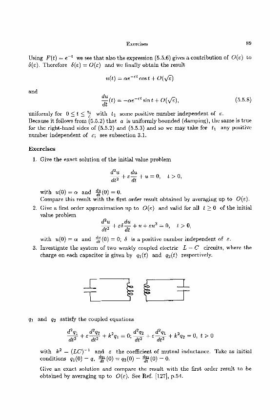
Exercises 89
Using F( t ) = e-' we see tha t also the expression (5.5.6) gives a contr ibut ion of 0(6) to 5(6). Therefore 5(6) = O(6) and we finally obtain the result
~(t) = ~-~' ~ost + O(v~)
and du dt (t) = - a e -Et sin t + O(v/~), (5.5.8)
uniformly for 0 _ < t < _ t_x with t l some positive number independent of 6. Because it follows from i5.5.2) tha t a is uniformly bounded (damping), the same is true for the r ight-hand sides of (5.5.2) and (5.5.3) and so we may take for t l any positive number independent of 6; see subsection 3.1.
Exerc i s e s
1. Give the exact solution of the initial value problem
d2u du dt 2 + 6 - d T + U = O , t > o ,
with u ( 0 ) = a and d~ ~(0)-0. Compare this result with the first order result obtained by averaging up to 0(6) .
2. Give a first order approximat ion up to O(6) and valid for all t >_ 0 of the initial value problem
d2u du dt-- T + 65-d- [ + u + eu 3 = 0 , t > O ,
with u ( 0 ) = c~ and d= -~-(0) -- 0; 5 is a positive number independent of 6.
3. Investigate the system of two weakly coupled electric L - C circuits, where the charge on each capacitor is given by ql(t) and q2(t) respectively.
ql and q2 satisfy the coupled equations
d2ql d2 q2 k2 d2 q2 d2 ql dt--- 5- + 6 ~ + q~ = O; - ~ + 6--d-- ~ + k2q2 = O, t > 0
with k 2 - (LC) -1 and 6 the coefficient of mutua l inductance. Take as initial d-~-(O) = q2(O) -- d-~(O) = O. conditions ql (0) = q, dt dt
Give an exact solution and compare the result with the first order result to be obtained by averaging up to 0(6) . See Ref. [127], p.54.
90 Chapter 5. The Method of Averaging
4. Investigate as in section 4.1 the weakly forced nonlinear oscillations of a "soft" spring, represented by the equat ion
d2u
dt 2 -Jr U - - ~ U 3 = r cos wt, A > 0
with CO 2 = 1 + ~#.
5. Investigate as in section 4.2 the weakly forced nonlinear oscillations of a "soft" spring with damping, represented by the equation
d2u
dt 2 du
+ r + u - r 3 = r cos~t , d t
A > 0
with w 2 = 1 + ~ # and ~ > 0 , independent of ~.
6. Investigate with the aid of averaging the forced nonlinear oscillations of a "hard" spring with damping, represented by the equation
d2u du + r + u + cu 3 - A cos wt,
dr---- ~ dt
with all three parameters ~ > 0, A > 0 and w independent of c. 1 i Take w ~ 0 A w ~ • 1 7 7
ii W h a t happens whenever w - 0 V w = + 3 V w - + ! ? 3 "
iii Consider also the case w = ~#.
Warning: this exercise takes much time.
C h a p t e r 6
T H E M E T H O D O F M U L T I P L E S C A L E S
1. I n t r o d u c t i o n
In the previous chapter we have investigated the approximation up to the first order of the Duffing equation
d2u -~- U -~- E U 3 - - 0 , (6.1.1)
dt 2
with the initial conditions u(0) = a and d~ - ~ ( 0 ) - 0. The result is given by (5.3.13)"
3a2et) + O(r (6.1.2) ~(t) = ~ cos(t +
t l uniformly valid for 0 <__ t < 7-, with tl some positive number independent of r
This result exhibits two so-called time scales: a "fast" time t and a "slow" time 7- - ct. The same phenomenon appears in the study of the perihelium precession determined by the equation
d2u dye--- 5 + u = a + cu 2, (6.1.3)
with the "initial" conditions u ( 0 ) = a and d~ ~(0) = ~. Formula (5.3.14) yields
u(O) -- a + V i a - a) 2 + 2~2 COS {0 - - acO - arctan ( a - - ~ ) } + O(~),
uniformly valid for 0 _< ~ < t~l, c
where 01 is some positive number independent of r Again we have two scales: a "fast" scale 0 and a "slow" one ~ = ~0. It is already a century ago that Lindstedt [98, 99] in his studies of celestial mechanics introduced explicitly different time scales in order to eliminate secular terms such as we have met in Chapter 3 in the construction of expansions of the solutions of (6.1.1) and (6.1.3). Another interesting equation with solutions exhibiting two time scales is given by the linear oscilator with weak damping.
d2u d u dt 2 + 2~-~- + u - 0, 0 < e << 1, (6.1.5)
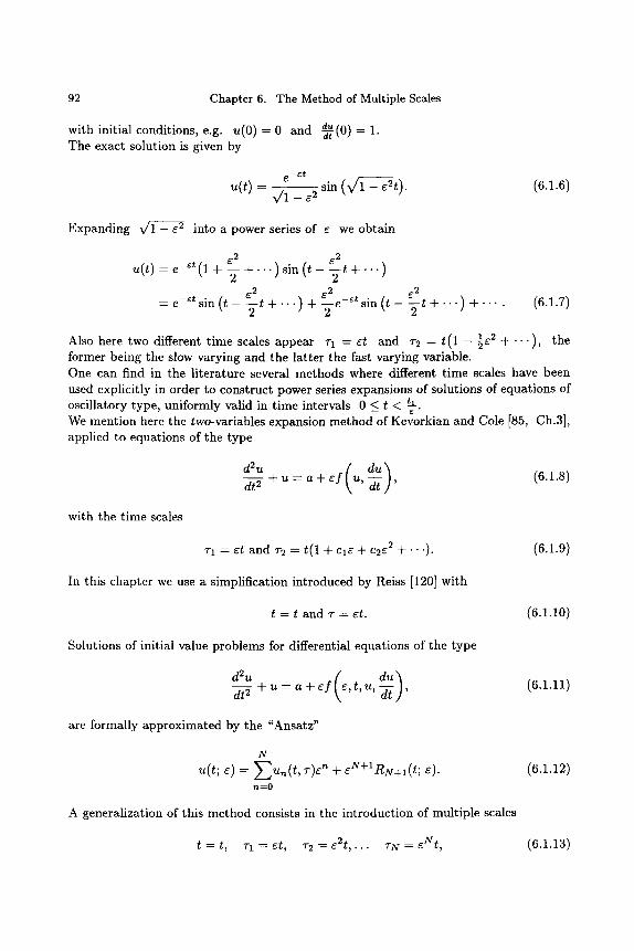
92 Chapter 6. The Method of Multiple Scales
with initial conditions, e.g. u(0) = 0 and d~ ~-(0) = 1. The exact solution is given by
--~t e sin (V/1 - e2t) (6.1.6)
u(t) = v/1 _ ~
Expanding v/1 - e 2 into a power series of e we obtain
6 2 6 2 u(t) = e -6t(1 + -~- + . - . ) s i n ( t - --fit + - . . )
= e -et sin (t - ~2 g.2 g.2 -2 t + " " " ) + - e - s t sin (t ~ t + . . . ) + " " . (6.1.7)
Also here two different time scales appear T 1 - - et and T2 = t ( 1 - 1 2 5e + . . . ) , the former being the slow varying and the latter the fast varying variable. One can find in the literature several methods where different time scales have been used explicitly in order to construct power series expansions of solutions of equations of oscillatory type, uniformly valid in time intervals 0 < t < ~ . We mention here the two-variables expansion method of Kevorkian and Cole [85, Ch.3], applied to equations of the type
d t - - - ~ + u = a + e f u , - ~ ,
with the time scales
T 1 - - et and T2 = t(1 + ClC -[- C2 g'2 - [ - ' " "). (6.1.9)
In this chapter we use a simplification introduced by Reiss [120] with
t = t and T = et. (6.1.10)
Solutions of initial value problems for differential equations of the type
d2u ( d u ) (6.1.11) dt--- ~ + u = a + e f e , t , u , - ~ ,
are formally approximated by the "Ansatz"
N u(t; C) = E u n ( t , T)C n + cN+IRN+I( t ; C).
n-~O
(6.1.12)
A generalization of this method consists in the introduction of multiple scales
t = t, T1 -- ~t, T2 = c2t,... TN -- ~Nt, (6.1.13)
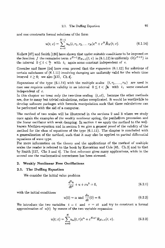
2.1. The Duffing Equation 93
and one constructs formal solutions of the form
N - 1
u(t; ~) = E u~(t, T1, T2,... TN)E ~ + eNRN(t; ~). (6.1.14) n--O
Kollett [87] and Smith [130] have shown that under suitable conditions to be imposed on the function f the remainder term sN+IRN+I(t; C) in (6.1.12)is uniformly O(c N+l) in the interval 0 < t < k with t l again some constant independent of ~.
Greenlee and Snow [54] have even proved that the expansion (6.1.12) for solutions of certain subclasses of (6.1.11) involving damping are uniformly valid for the whole time interval t _ 0; see also [127, Ch.4].
Expansions of the type (6.1.14) with the multiple scales (t, T1,..., TN) are used in case one requires uniform validity in an interval 0 ~ t < ~ with t l some constant independent of ~. In this chapter we treat only the two-time scaling (t,~t), because the other methods are, due to many but trivial calculations, rather complicated. It would be worthwhile to develop software packages with formula manipulation such tha t these calculations can be performed with the aid of a computer.
The method of two scales will be illustrated in the sections 2 and 3 where we study once again the examples of the weakly nonlinear spring, the perihelium precession and the linear oscillator with weak damping. In section 4 we apply the method to the well- known Mathieu-equation and in section 5 we give a general proof of the validity of the method for the class of equations of the type (6.1.11). The chapter is concluded with a generalization of the method, such tha t it may also be applied to partial differential equations of wave type. For more information on the theory and the applications of the method of multiple scales the reader is referred to the book by Kevorkian and Cole [85, Ch.3] and to that by Smith [127, Chs 3 and 4]. The first reference gives many applications, while in the second one the mathematical correctness has been stressed.
2. W e a k l y N o n l i n e a r F ree Oscillations
2.1. T h e Duff ing Equation
We consider the initial value problem
d2u + u + cu 3 = 0,
dt 2
with the initial conditions
(6.2.1)
N
u(t; ~) = ~-~un(t, r)e" + eN+~RN+~(t; ~). (6.2.3) r~--O
d u u(0) = a and -d-/(0) = 0. (6.2.2)
We introduce the two variables t = t and w = st and try to construct a formal approximation of u(t) by means of the two variable expansion
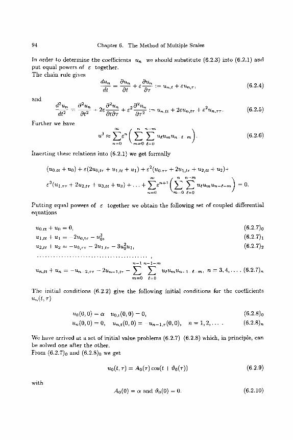
94 Chapter 6. The Method of Multiple Scales
In order to determine the coefficients u~ we should substitute (6.2.3) into (6.2.1) and put equal powers of e together. The chain rule gives
d u n O u r Oun d t = Ot + e--~T "= un , t + eu,~,r, (6.2.4)
d2 un C~2 ?~n
d t 2 Ot 2
and
Further we have
02Un "C 2 0272n + 2eO--~T + 0~_2 := Un,tt n u 2eUn, tr + e2Un,rr .
~
n = 0 m = 0 t = 0
Inserting these relations into (6.2.1) we get formally
(6.2.5)
(6.2.6)
(~o,. + ~o) + ~(2~o,~. + ~ , . + u~) + ~(uo, . . + 2~,~. + ~ , . + ~ ) +
) e3(Ul,~-~ - Jr- 2Zt2,t~- -Jr- U3,tt Jr- Zt3) -~ - . . . -~ - ~ g . n + l Ug't tmltn_g_ m -- O.
n=O -- t=O
Put t ing equal powers of e together we obtain the following set of coupled differential equations
UO,tt n c Uo = O,
Ul, t t -~- Ztl ~ --2Uo,tr -- U 3,
U2,tt n c U 2 = --UO,rr -- 2Ul , t r -- 3U2Ul~
(6.2.7)o
(6.2.7)1
(6.2.7)2
n--1 n - - l - -m
Un,tt n t - t tn = --Un-2,r~- -- 2 l t n - l , t r -- ~ ~ U l U m U n - l - f . - m , n = 3 , 4 , . . . . ( 6 . 2 . 7 ) n
m = 0 l=0
The initial conditions (6.2.2) give the following initial conditions for the coefficients ~. ( t , ~)
~o(0, 0) = ~ ~o,~(0, 0) = 0, ~ ( 0 , 0) = 0, u.,~(0, 0) = - ~ . _ ~ , . ( 0 , 0),
(6.2.8)0 n = 1 , 2 , . . . . (6.2.8)n
We have arrived at a set of initial value problems (6.2.7)-(6.2.8) which, in principle, can be solved one after the other. From (6.2.7)0 and (6.2.8)0 we get
uo( t , T) = AO(T) cos ( t + v~0(~')) (6.2.9)
with Ao(0) = a and ~o(0) = 0. (6.2.10)
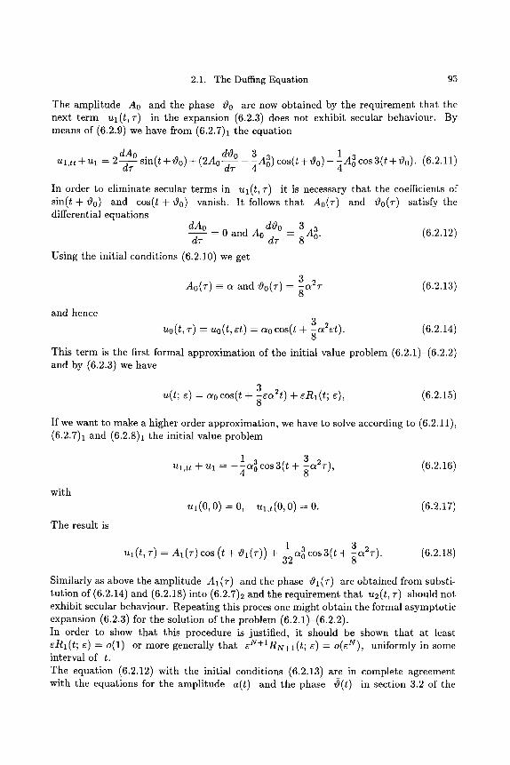
2.1. The Duffing Equation 95
The amplitude A0 and the phase zg0 are now obtained by the requirement that the next term ul(t, T) in the expansion (6.2.3) does not exhibit secular behaviour. By means of (6.2.9) we have from (6.2.7)1 the equation
2 dA~ dig~ - A 3) cos(t + tgo)- ~A ] cos3(t + t9o) (6.2.11) Ul,tt + ?.t 1 - - ~ sin(t + ~0) + ( 2 A 0 ~ -
In order to eliminate secular terms in ul(t,v) it is necessary that the coefficients of sin(t + tg0) and cos(t +~ It follows that Ao(T) and ~0 (T) satisfy the differential equations
dAo = 0 and Ao d~~ - -8 A]. (6.2.12)
d~
Using the initial conditions (6.2.10) we get
3 Ao(T)--~ and ~)0(T)= ~a2T (6.2.13)
and hence 3a2et) (6.2.14) ~0(t, ~) - ~0(t, ~t) = ~0 cos(t + ~
This term is the first formal approximation of the initial value problem (6.2.1)-(6.2.2) and by (6.2.3) we have
.2 u(t; ~) - a0 cos(t + 8sa2t) + ~Ri(t; ~), (6.2.15)
If we want to make a higher order approximation, we have to solve according to (6.2.11), (6.2.7)1 and (6.2.8)1 the initial value problem
with
The result is
?-tl,tt Jr- Ul = ---~Ol 0 cos3(t + a2T), (6.2.16)
U 1 (0, 0) - - 0, U l , t ( 0 , 0) = 0. (6 .2 .17 )
Ul(t,T)=AI(T)COS(t+~)I(T))+-~aoCOS3(t+ a2T). (6.2.18)
Similarly as above the amplitude A1 (T) and the phase ~91 (T) are obtained from substi- tution of (6.2.14) and (6.2.18) into (6.2.7)2 and the requirement that u2(t, T) should not exhibit secular behaviour. Repeating this proces one might obtain the formal asymptotic expansion (6.2.3) for the solution of the problem (6.2.1)-(6.2.2). In order to show that this procedure is justified, it should be shown that at least CRl(t; r = o(1) or more generally t h a t ~ N + I R N + I ( t ; ~) = o ( r uniformly in some interval of t. The equation (6.2.12) with the initial conditions (6.2.13) are in complete agreement with the equations for the amplitude ~(t) and the phase ~(t) in section 3.2 of the
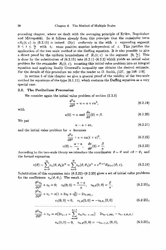
96 Chapter 6. The Method of Multiple Scales
preceding chapter, where we dealt with the averaging principle of Krilov, Bogoliubov and Mitropolski. So it follows already from this principle that the remainder term eRl(t; e) in (6.2.15) is indeed O(e) uniformly in the with e expanding segment 0 < t < ~ with t l some positive number independent of e. This justifies the application of the two scale method in the Duffing equation. It is also possible to give a direct proof for the uniform boundedness of R l ( t ; e) in the segment [0, ~]. This is done by the substitution of (6.2.15) into (6.2.1)-(6.2.2) which yields an initial value problem for the remainder R1 (t; e); recasting this initial value problem into an integral equation and applying finally Gronwall's inequality one obtains the desired estimate. For the details of this procedure we refer the reader to D. Smith, [127, pp.106-116].
In section 5 of this chapter we give a general proof of the validity of the two-scale method for equations of the type (6.1.11), which contains the Duffing equation as a very special case.
2.2. The Per ihe l ium Precess ion
with
We put
We consider again the initialvalue problem of section (5.3.3) d2u
-4- u = a + CU 2, dO 2
du u(O) = cr and ~-~(0) = ~.
(6.2.19)
(6.2.20)
(6.2.21) ~z = a ff-all ,
and the initial value problem for v becomes d2v dO--- ~ -4- v = ea(1 + v) 2, (6.2.22)
v ( O ) = ~ -a a __d ~gd v (0) = -'/~a (6.2.23)
According to the two-scale theory we introduce the coordinates t9 = t9 and et9 = tgl and the formal expansion
e~ N
v(tg) ~ ~- '~v,~(~,tgl)e" = Z v , . , ( O , ~ l ) e " + e N + I R N + I ( ~ ; e). (6.2.24) n=O n=O
Substitution of this expansion into (6.2.22)-(6.2.23) gives a set of initial value problems for the coefficients vn (vg, 01). The result is
02vo ~ - a ~ , 0t92 + vo = O; vo(O, O) = ~ ' a Vo,~(O, O) = -a (6.2.25)0
02v l 0~9---- ~ -4- Vl = a(1 + 2v0 + v 2) - 2v0,~1,
vx(O, O) = O, Vl,o(O, 0) = -v0,~l (0, 0) (6.2.25)1
r t --1 02Vn + Vn --a(2Vn--1 -4- y ~ VmVn-- l - -m)- 2Vn--l,tg#,- Vn--2,tg,tg,;
tn--O
vn(O, O) = O, vn,9(O, O) = -v,~-l,9~ (0, 0), (6.2.25)2
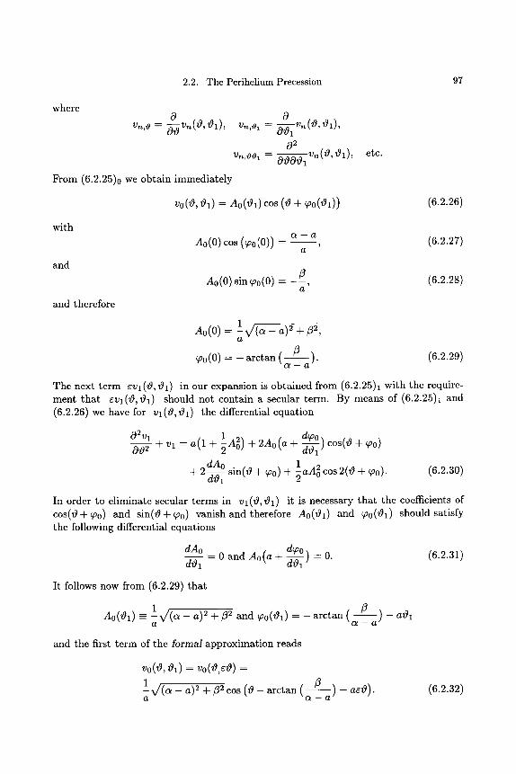
2.2. The Perihelium Precession 97
where 0
Vn,z9 : - ~ Vn ( t~ , t91), 0 ~,,~ = b-~l v,(O, ~1),
0 ~ ~ v ~ ( ~ , ~ l ) ,
From (6.2.25)0 we obtain immediately
etc.
vo(~, ~1) = Ao(~l)cos (~ + qOo(t91)) (6.2.26)
with
and
and therefore
Ao(0) cos (r = a - a (6.2.27) a
Ao(0) sin ~o(0) = -fl-- (6.2.28) a
A o ( 0 ) = 1V/(a a)2+f12 a
). ~o(0) = - arctan ( a a (6.2.29)
The next term GV 1 (V q, ~ql) in our expansion is obtained from (6.2.25)1 with the require- ment that r ~1) should not contain a secular term. By means of (6.2.25)1 and (6.2.26) we have for vl (zg, ~1) the differential equation
02vl 0v~----- 5- + Vl = a(1 4- ~Ao 2) + 2Ao(a 4- ~10 ) cos(v q + r
1 2 dAo s in(O+ ~o) + -~aAo cos 2(t~ + ~oo). + 2-j5~- ~ (6.2.30)
In order to eliminate secular terms in Vl (v~, ~1) it is necessary that the coefficients of cos(~+qo0) and s i n ( t g + ~ o ) v a n i s h and therefore Ao(~l) and qoO(~l)shouldsat isfy the following differential equations
dAo dr91
d~o) = 0 a n d A o ( a + ~ = 0 . (6.2.31)
It follows now from (6.2.29) that
) - a ~ l 1 t32 (vQ1) = arctan ( a a do(z91) = - V/(a - a) 2 n t- and ~oo - a
and the first term of the formal approximation reads
,o(~, ~1) = , o ( ~ , ~ ) =
fl ) - e e l ) . 1 V/(a _ a) 2 + Z2 cos (t9 - arctan ( a a a
(6.2.32)
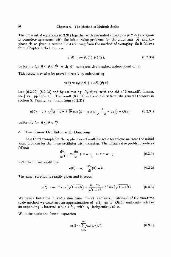
98 Chapter 6. The Method of Multiple Scales
The differential equations (6.2.31) together with the initial conditions (6.2.29) are again in complete agreement with the initial value problems for the ampl i tude A and the phase ~ as given in section 5.3.3 result ing from the method of averaging. So it follows from Chapte r 5 tha t we have
, (o ) - ~o(O, o, ) + o(~), (6.2.33)
uniformly for 0 < 0 < ~ with 01 some positive number, independent of e.
This result may also be proved directly by subs t i tu t ing
v(0) = v0(0, 01) + 8Rx (0; E)
into (6.2.22)-(6.2.23) and by es t imat ing R1(0; e) with the aid of Gronwall 's lemma, see [127, pp.106-116]. The result (6.2.33) will also follow from the general theorem in section 5. Finally, we obta in from (6.2.21)
u(0) = a + V/(a - a) 2 +/32 cos (0 - arc tan ~ - C l ~ - - a
aeO) + O(e), (6.2.34)
uniformly for 0 < 0 < ol
3. T h e L i n e a r Oscillator with Damping
As a third example for the application of mult iple scale technique we t reat the initial value problem for the linear oscillator with damping. The initial value problem reads as follows
d2u du dt---- ~ + 26-~- + u = O, 0 < ~ << 1, (6.3.1)
with the initial conditions d u
~(0) = ~, ~ ( 0 ) = b. (6.3.2)
The exact solution is readily given and it reads
u(t) -= ae -~t cos (V/1 -- r + b + ea -~t ~,/y_z~_~ ~ si~ ( v q - ~ t ) (6.3.3)
We have a fast t ime t and a slow t ime T = r and as a i l lustrat ion of the two-time scale me thod we construct an approximat ion of u(t) up to O(~), uniformly valid in an expanding t-interval 0 < t < t~ with t l independent of r
We make again the formal expansion
oo
u(t) ~ y~u, , ( t , T)e n, (6.3.4) n--O
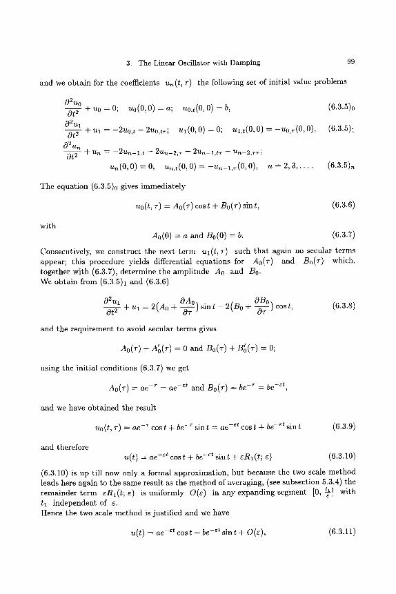
3. The Linear Oscillator with Damping 99
and we obtain for the coefficients u,~ (t, T) the following set of initial value problems
02Uo
Ot 2
0 2 u l
Ot 2
02 ?Jtn
+ u0 = 0; uo(0,0) = a; u0,t(0,0) = b, (6.3.5)0
-~- ~tl = --2U0,t -- 2U0,tr ; Ul (0, 0) "-- 0; Ul , t (0 , 0) = - -U0 , r (0 , 0) ,
Ot---- 5- + u,~ = - 2 u n - l , t - 2Un-2 ,r - 2 U n - l , t r - Un--2,TT;
u~(0, 0) = 0, ~ ,~ (0 , 0) = - ~ _ ~ , ~ ( 0 , 0),
(6.3.5)1
n -"- 2, 3 , . . . . (6.3.5)n
The equation (6.3.5)o gives immediately
uo(t , T) = AO(T) cos t + Bo(~') sin t, (6.3.6)
with A0(0) = a and Bo(0) = b. (6.3.7)
Consecutively, we construct the next term u l ( t , T) such that again no secular terms appear; this procedure yields differential equations for Ao(~-) and B0(~-) which, together with (6.3.7), determine the amplitude A0 and B0. We obtain from (6.3.5)1 and (6.3.6)
0 2 u l O A o ) OBo Ot---- 5- + U l ---- 2 (Ao + ~ sin t - 2 (Bo + ~ ) c o s t, (6.3.8)
and the requirement to avoid secular terms gives
AO(T) + A~o(T) -- 0 and B o ( r ) + B~o(T) -- 0;
using the initial conditions (6.3.7) we get
Ao(T) = a e - " = ae - s t and B0(~') = be - r = be - s t ,
and we have obtained the result
uo(t, r) = ae - ~ cost + be - ~ sint = ae - s t cost + be - s t sint (6.3.9)
and therefore u( t ) = ae - s t cos t + be - s t sin t + oR1 (t; ~) (6.3.10)
(6.3.10) is up till now only a formal approximation, but because the two scale method leads here again to the same result as the method of averaging, (see subsection 5.3.4) the remainder term ~R1 (t; e) is uniformly O(e) in any expanding segment [0, t~] with tl independent of e. Hence the two scale method is justified and we have
u( t ) = ae -Et cos t + be - s t sin t + O(e), (6.3.11)
100 Chapter 6. The Method of Multiple Scales
uniformly for 0 < t < Lt with t l an arbitrary number independent of 6. It is also possible to prove directly that R1 (t; 6) is uniformly bounded for all t _ 0; since this direct proof is relatively simple for our linear initial value problem, we give it right here. Inserting (6.3.10)into (6.3.1)-(6.3.2)we get for Rl(t; 6) the initial value problem
d2R1 dR1 dr---- if- + 2 6 ~ + R1 = 6(ae -~t cos t + be -~t sin t), (6.3.12)
with dR1 (0; 6) = a. (6.3.13) RI(0; 6) = 0 and
Since u(t) exists for all values of t the same is also true for Rl(t ; 6). To simplify the calculations we put
R1 (t; e) = e-erR1 (t; 6), (6.3.14)
and /~1 satsfies the initial value problem
d 2 / ~ 1
dt 2 + R1 = 6(acost + bsint) + 62kl, (6.3.15)
with
d/~l (0; 6) = a. Rl(O; 6) = 0 and - ~ -
Variation of constants gives for 1)1 the integral equation
(6.3.16)
t
/~1 (t; e) = a sin t + e / ( a cos r + b sin T) sin(t -- ~')dT
0
t
+ 62 / 1)l(r; 6)sin(t -- r)dr.
0
From this equation it follows that
t
Ik~(t; ~)1 < I~1 + ~(1~1 + Ibl)t + ~ f Ih~(~; ~)ld~ 0
o r
I/)l (t; 6)1 + (lal + Ibl) _< lal + (lal + Ibl)+ t
+ e / { I/~I(T, 6)1 + (lal + Ibl)}dT.
0
Applying Gronwall's lemma (Lemma 3, Chapter 3) we get
I/~l(t; e)J + (]aJ + ]bl) < { la] + (la] + ]bl) } exp[6t],
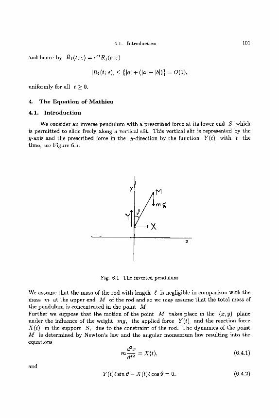
4.1. Introduction 101
and hence by n i ( t ; e) = er ~)
IRl(t; c)l < {lal + (lal + Ibl)} = O(1),
uniformly for all t _> 0.
4. The Equation of Math ieu
4.1. Introduct ion
We consider an inverse pendulum with a prescribed force at its lower end S which is permitted to slide freely along a vertical slit. This vertical slit is represented by the y-axis and the prescribed force in the y-direction by the function Y(t) with t the time, see Figure 6.1.
Y M
Fig. 6.1 The inverted pendulum
We assume that the mass of the rod with length I is negligible in comparison with the mass m at the upper end M of the rod and so we may assume that the total mass of the pendulum is concentrated in the point M. Further we suppose that the motion of the point M takes place in the (x, y) plane under the influence of the weight mg, the applied force Y(t) and the reaction force X(t) in the support S, due to the constraint of the rod. The dynamics of the point M is determined by Newton's law and the angular momentum law resulting into the equations
d2x r n ~ = X(t), (6.4.1)
and
Y(t ) t~s in~- X(t)~ cos z9 = 0. (6.4.2)
102 Chapter 6. The Method of Multiple Scales
The latter equation results from the fact that the moment of inertia about the centre of gravity M is zero. Assuming that the deviation ~ from equilibrium is small, we get after linearization
m i ~ - Y(t)t9 = O.
Putt ing the applied force Y( t ) equal to
Y( t ) = m g - rap(t)
we get finally the equation
g ~ (6.4.3)
In case p(t) is periodic the linear equation (6.4.3) is known as Hill's equation, usually written in the form
d2w + q(t)w = 0 (6.4.4)
dt 2
with q(t) periodic. If p(t) =_ 0 the solution of (6.4.3) is unbounded and the equilibrium solution 0 = 0 is unstable. Nevertheless, it is possible to choose the periodic function p(t), such that a bounded stable solution exists. Considering a normal pendulum, not upside down, the term -}v~ in equation (6.4.3) changes its sign and the equilibrium solution 0 = 0 is stable. Mutatis mutandis it is again possible to choose a periodic p(t), such that an unbounded unstable solution exists.
In this section we consider in particular the equation
d2u dt--- $ + (5 + e cos t)u = O, (6.4.5)
where 5 and e are parameters with 0 < e << 1. The equation is Mathieu's equation and it has, as we will see, very interesting properties. As to the periodicity and the stability of its solutions, we have at our disposal the theory of Floquet, concerning linear ordinary differential equations with periodic coefficients. Since this section is only meant to illustrate the method of two time scales, it is outside the scope of this chapter to give a detailed t reatment of Floquet 's theory. Instead we give in the sections 4.2 and 4.3 the results and we refer the reader to lit.J131], where Floquet 's theory for second order equations is t reated in detail and where the stability of solutions of Hill's equation is discussed.
4.2. Floquet's Theory for Linear Equations with P e r i o d i c Coef f ic ien t s
We consider the equation
d2w dw dz--- ~ + p(z)-~z + q(z)w = 0 (6.4.6)
with p and q periodic with real period w and analytic in a strip containing the real axis, (z - x + iy). Although the equation (6.4.6) is periodic, a solution does not need to
4.3. Application to Hill's Equation 103
be periodic. Suppose the functions wl(z), w2(z) form a fundamental set of solutions of (6.4.6); because wl (z + w) and w2(z + w) are also solutions, we have the relations
Wl(Z -~- w) z allWl(Z) -~- a12w2(z),
w2(z + w) = a21wl (z) + a22w2(z),
with aij constant. The problem to determine a set such tha t
wi(z + w) = orwi(z), i = 1 , 2
leads to the necessary condition
a l l - - or a 1 2 z 0 ,
a 2 1 a 2 2 - - or (6.4.7)
which is called the characteristic equation. There are now two possibilities
i) The equation (6.4.7) has two different roots
a i = e ~ , i = 1 , 2 .
There exist two independent so-called normal solutions, which have the form
~ , (z ) = ~ , ~ , ( z ) (6.4.s)
with ~, (z + w) = ~,(z) and c~1 ~ c~2. ii) The equation (6.4.7) has a double root. There exists only one normal solution
wl = e ~ lz~l (z ) and the other solution independent of wl has the form
a z w2(z) = e ~lz { ~ w ~ l (z) + r (z) } (6.4.9)
with r (z + w) = r
The solutions of (6.4.6) are called stab/e, if all solutions remain bounded for all real positive values of z, and unstable otherwise, i.e. if there exists a solution which is not bounded for x --+ +oo. In case i) we have stabil i ty for Re c~i < 0, i - 1, 2 and instabili ty otherwise; in case ii) we have stabil i ty for Re c~1 < 0, a ~ 0 or Re c~1 < 0, a - 0 and instabil i ty otherwise.
4.3. Appl icat ion to Hill's Equation
The equation (6.4.6) takes the part icular form
d2w dz---- ~ + q(z)w - 0 (6.4.10)
with q(z -F w) -- q(z).
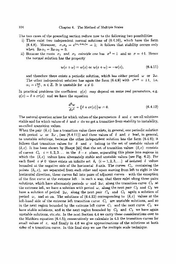
104 Chapter 6. The Method of Multiple Scales
The two cases of the preceding section reduce now to the following two possibilities i) There exist two independent normal solutions of (6.4.10), which have the form
(6.4.8). Moreover, ala2 - e (~1+~2)~ = 1; it follows tha t stabili ty occurs only when Re O~ 1 = Re a2 = 0.
ii) Because the roots a l and a2 coincide one has a 2 = 1 and so a = :kl. Hence the normal solution has the proper ty
w(z + w) = w(z) or w(z + w) = - w ( z ) , (6.4.11)
and therefore there exists a periodic solution, which has either period w or 2w. The other independent solution has again the form (6.4.9) with e al~ - =kl, i.e.
i mr a l = ~ , n C Z . It is unstable for a ~ 0 .
In practical problems the coefficient q(z) may depend on some real parameters , e.g. q(z) = 5 + cr(~z) and we have the equat ion
d 2 w + {5 + cr(z)}w = O. (6.4.12)
dz 2
The na tura l question arises for which values of the parameters 5 and r are all solutions stable and for which values of 5 and r do we get a transition from stabili ty to instability, so-called transition values. When the pair (5, r has a t ransi t ion value there exists, in general, one periodic solution with period w or 2w , (see (6.4.11)) and these values of 5 and r lead, in general, to unstable solutions, because the other independent solution has the form (6.4.9); it follows tha t t ransi t ion values for 5 and r belong to the set of unstable values of (5, r It has been shown by Haupt [65] tha t the set of t ransi t ion values (5, r consists of curves Ci i - 1, 2, 3 . . . in the 5 - r plane, separat ing this plane into regions in which the (5, r values have a l ternate ly stable and unstable values (see Fig. 6.2). For each fixed r =p- 0 there exists an infinite set 5i (i - 1, 2, 3 , . . . ) of isolated 5 values bounded at the negative side of the horizontal 5-axis. The curves Ci, containing the points (5i, r are separated from each other and upon moving from left to right in the horizontal direction, these curves fall into pairs of adjacent curves - with the exception of the first curve at the extreme left - in such a way, tha t there exist along these pairs solutions, which have a l ternate ly periods w and 2w; along the t ransi t ion curve C1 at the extreme left, we have a solution with period w, along the next pair C2 and C3 we have a solution of period 2w, along the next pair C4 and C5 again a solution of period w, and so on. The solutions of (6.4.12) corresponding to (5,r values at the left-hand side of the ext reme left t ransi t ion curve C1 are unstable solutions, and so in the next region bounded by the ext reme left curve C1 and the next curve C2 we have stable solutions, and in the next region bounded by C2 and C3 we have again unstable solutions, etc.etc. In the next Section 4.4 we carry these considerations over to the Mathieu equat ion (6.4.5); consecutively we calculate in 4.5 the t ransi t ion curves for small values of r and finally in 4.6 we give approximations of the solutions at both sides of a t ransi t ion curve. In this final step we use the multiple scale technique.
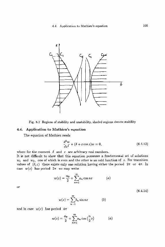
4.4. Application to Mathieu's equation 105
C, C~
Fig. 6.2 Regions of stability and unstability, shaded regions denote stability
4.4. A p p l i c a t i o n to Mathieu's equation
The equation of Mathieu reads
d2w + (5 + e cos z)w = 0, (6.4.13) dz 2
where for the moment 5 and e are arbi t rary real numbers. It is not difficult to show tha t this equat ion possesses a fundamental set of solutions Wl and w2, one of which is even and the other is an odd function of z. For t ransi t ion values of (5, e) there exists only one solution having either the period 2 r or 4r . In case w(z) has period 2~ we may write
o o
a0 ~(z) = ~ + a~ r (a) n - - 1
o r
o o
w(z) = E b n s innz n--'l
and in case w(z) has period 4Ir
(b)
(6.4.14)
o o a 0 n +
n - - 1
(a)
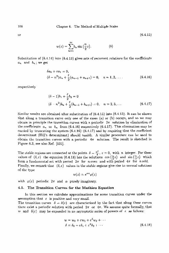
106 Chapter 6. The Method of Multiple Scales
or (6.4.15)
w(z) = E b n sin ( 2 z ) . (b) n - - 1
Subst i tut ion of (6.4.14) into (6.4.13) gives sets of recurrent relatiops for the coefficients an and bn ;we get
5no + gal = O,
(~ - ~ ) a . + ~(a._~ + a .+ l ) - O, n = 1 , 2 , . . . . (6.4.16)
respectively
( 6 - 1)bl + ~b2 = 0
(b._ + b . + 1 - 0 ( 5 - n2)b,~ + ~ 1 1 , n = 2, 3 , . . . (6.4.17)
Similar results are obtained after subst i tut ion of (6.4.15) into (6.4.13). It can be shown tha t along a t ransi t ion curve only one of the cases (a) or (b) occurs, and so we may obtain in principle the t ransi t ion curves with a periodic 2 r solution by elimination of the coefficients an or bn from (6.4.16) respectively (6.4.17). This elimination may be carried by t runcat ing the system (6.4.16)-(6.4.17) and by requiring tha t the coefficient de terminant (Hill's determinant) should vanish. A similar procedure can be used to obtain the t ransi t ion curves with a periodic 47r solution. The result is sketched in Figure 6.3, see also Ref. [131].
n 2 The stable regions are connected at the points 5 - -~-, ~ = 0, with n integer. For these values of (6, e) the equation (6.4.13) has the solutions cos (2 z) and sin (~z) which form a fundamental set with period 21r for n even and with period 47r for n odd. Finally, we remark tha t (5, ~) values in the stable regions give rise to normal solutions of the type
w(z) = e ~ ( z )
with ~(z) periodic 27r and a purely imaginary.
4.5. T h e T r a n s i t i o n C u r v e s for t h e M a t h i e u E q u a t i o n
In this section we calculate approximations for some transi t ion curves under the assumption tha t ~ is positive and very small. The transi t ion curves 6 = 5(~) are characterized by the fact tha t along these curves there exist a periodic solution with period 21r or 4~r. We assume quite formally, tha t w and 5(~) may be expanded in an asymptot ic series of powers of ~ as follows:
w = w 0 -~ ~Wl -~- c 2w2 -~-'-"
5 "-- 5 0 + C 5 1 -~- C 2 5 2 -~-- " " " (6.4.18)
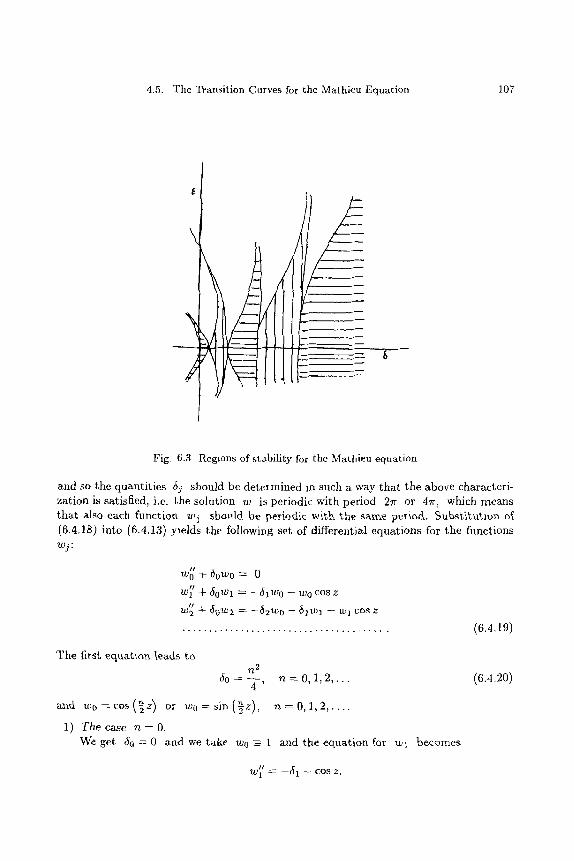
4.5. The Transition Curves for the Mathieu Equation 107
\
Fig. 6.3 Regions of stability for the Mathieu equation
and so the quantities by should be determined in such a way that the above characteri- zation is satisfied, i.e. the solution w is periodic with period 21r or 47r, which means that also each function w~ ~hauld be periodic w~tk the sam~ period. Substitution o~ (6.4~18) into (6.4.13) yields the fbllowiug set of differential equations for the functions wj:
/ /
Wo +50w0 = 0 l /
w l + 6oWl -- - 6 1 w o - wo cos z l /
(6.4.19)
The first eclu~t~ou [~ads to n 2
J0=--~-, n = 0 , 1 , 2 , . . .
~ ~ o = ~o~ ( ~ z ) o~ ~ 0 = ~ ( ~ z ) , ~ = 0, ~, ~ , . . . .
1) T h e case n = 0 . We get 6 0 = 0 and we take w 0 ~ 1 and the equ~t~o~ for wl becomes
(6.4.20)
// ~ --(~I -- COS Z. W I
108 Chapter 6. The Method of Multiple Scales
Because wl should be periodic, we have to e l iminate the secular t e r m and so we
are b rought to the requ i rement t ha t 51 = 0 and we get
~ 1 ( z ) = c o s z + ~,
where c is the cons tan t of integrat ion. The equat ion for w2 becomes now
" - ~ 2 - c o o s z - ( r z) 2 W 2 ----
(1 1 2z), = - 6 2 - c c o s z - + ~ c o s
f rom which we ob ta in due to the required per iodici ty of w2 t h a t 62 = - � 8 9 So we have got up to t e rms of the second order in c.
l e2 (6.4.21) 5 = - ~ + . . .
and along the t rans i t ion curve corresponding wi th this a p p r o x i m a t i o n we have as a p p r o x i m a t i o n of a periodic solut ion
w = 1 + e cos z, (6.4.22)
where we have taken c = 0.
The 1. z ) c a s e n =
1 Z 2; We have 50 - - 4 and w 0 - c o s ~ or w 0 - s i n
If we take Z
W 0 = COS 2 '
we ob ta in for wl the equa t ion
,, 1 z z W 1 q- ~ W 1 ---- - -61 COS ~ -- (COS ~ ) ( C O S Z )
z _ l z ----- ( -- 61 -- 1 ) COS ~ ~ COS 3 2 .
1 and we Avoiding the occurrence of a nonper iodic t e rm we should require 51 - - ~ get as a p p r o x i m a t i o n for the t rans i t ion curve
1 1 5 = ~ - ~e + . . . (6.4.23)
along which we have a 4 r periodic solut ion
W : C O S - - z (1 z) 2 t-e cos 2 4 - - - - . ( 6 . 4 . 2 4 )
4.5. The Transition Curves for the Mathieu Equation 109
z If we take w0 - sin ~ we obtain similarly
1 1 ~= ~ + ~ + . . . (6.4.25)
and z z) w - - s i n ~ + ~ s in3~ + . . . . (6.4.26)
3) The case n = 2.
We now have 5 0 - 1 and again the two cases w0 - c o s z and w 0 - sin z. Taking w0 = cos z we obtain for Wl the equat ion
,, _ (cos z) 2 W l ~t_ W l - - ( ~ 1 C O S Z - - = 1 1
- - - - - (~1 C O S Z 2 2
- - cos 2z.
El iminat ion of the secular t e rm gives 51 - 0 and
1 1 w l = - ~ -~ 6 cos2z.
Inserting these results into the equation for w2 we get
1 1 ! ! w~ + ~ = - ~ cos z - ( ~ + g cos 2z) cos z
1 = ( - 5 2 ) cos z - 1--2 cos 3z.
It follows tha t the formal approximat ion for the t ransi t ion curve is given by
5 = 1 + 5 e 2 + . . . (6.4.27)
with the 21r periodic solution
1 1 2z) + ~ ( z ) = ~os z + ~ ( - ~ + ~ cos . . . . (6.4.28)
Similarly, we obtain for w0 = sin z the approximations
5 = 1 - 1 E 2 + . - . (6.4.29) 12
with 1
w(z ) -- s inz + e (~ sin2z) + . - . . (6.4.30)
All these results are in agreement with the results of Haupt as s ta ted in the preceding section and a sketch of the approximate t ransi t ion curves is given in Figure 6.4.
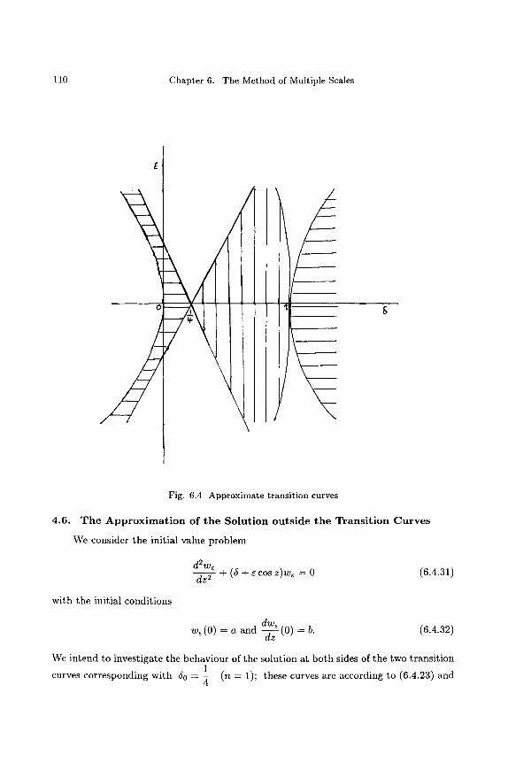
110 Chapter 6. The Method of Multiple Scales
/
\
Fig. 6.4 Approximate transition curves
4 .6 . T h e A p p r o x i m a t i o n o f t h e S o l u t i o n o u t s i d e t h e T r a n s i t i o n C u r v e s
We consider the initial value problem
d2we dz 2
+ (5 + E cos z)w~ = 0 (6.4.31)
wi th the initial condit ions
dw~ we(0) = a and --~z (0) = b. (6.4.32)
We intend to invest igate the behaviour of the solution at bo th sides of the two t rans i t ion
1 (n 1) these curves are according to (6.4.23) and curves corresponding wi th 50 = ~ = ;
4.6. The Approximation of the Solution outside the Transition Curves 111
1 1 (6.4.25) approximated by 5 - ~ T ~e. The calculations for other transition curves are
omitted, because these run along similar lines. Introduction of the two scales
= ez and 7/= z
transforms the initial value problem into the following initial value problem for the function w(~, 7/) = w(ez, z) := we(z)
e2 0 2w 02w 02w + 2e OfOrj + ~ + (5 + e cos ~)w - 0 (6.4.33)
with the initial conditions
and
Taking
and assuming
w(O, O ) = a
Ow OW)(o,o) -- b.
5 = 1 - q- 851 q- e252 q - . . . , 4
W(~, 7/) : WO(~, 7/) -~" ~W 1 (~, 7/) -~- �9 " " ,
we get the following recursive set of initial value problems for w0, Wl , . . .
(6.4.34)
02 wo 1 ~_~ 0712 + -~wo = O, wo(O, O) -- a, (O, O) - b, (6.4.35)
with
02Wl 1 02w~ - (51 + cos r/)wo, Oo?,]-------- ~ + ~w I -- -20~Or/
o ~ (0, 0) = o~0 (0, 0) W l ( 0 , 0 ) ---- 0 and ~ - - - ~ ,
etc. Solving (6.4.35) we obtain
(6.4.36)
wo(~, 7/)= A0(~)cos (~rl) + B0(~)sin ( ~ ) (6.4.37)
with A0(0) = a and B 0 ( 0 ) = 2b. (6.4.38)
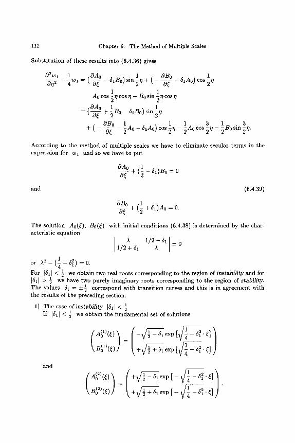
112 Chapter 6. The Method of Multiple Scales
Substitution of these results into (6.4.36) gives
1 iOAo 1 OBo 02Wl + Wl --" t -- (~IBo) sin ~'7 + (
1 1 - A0 cos ~ 77 cos 77 - B0 sin ~ 77 cos 77
00_~~0 21 21 - ( - - + Bo - ( ~ l B o ) sin 7/
, OBo 1 +
1 6z Ao) cos ~ 7/
0~ 2
1 1 3 1 3 Ao - 61Ao) cos ~ r / - ~ Ao cos ~ r / - ~ Bo sin ~ 77.
According to the method of multiple scales we have to eliminate secular terms in the expression for wz and so we have to put
OAo 1 O---~ + ( 2 -- ~ I )Bo = 0
and (6.4.39)
OBo 1 O~ -[- (2 -[- ~I)A~ -- 0.
The solution A0(~), B0(~) with initial conditions (6.4.38) is determined by the char- acteristic equation
A 1 / 2 - ~ 1 _ 0 1/2 +6z A
1 or A 2 - (~-612 ) = 0 .
1 For [61[ < ~ we obtain two real roots corresponding to the region of instability and for z [6t[ > ~ we have two purely imaginary roots corresponding to the region of stability.
1 correspond with transition curves and this is in agreement with The values 6z - =k the results of the preceding section.
1 1) The case of instability [61[ < 5 1 If [~1[ < ~ we obtain the fundamental set of solutions
(A(1)(~)/ = /-r / Bo(1) (~) + g / 1 + ~1 exp [ V / ~ - ~12 ~]
and +lexpE +1/ - - - o
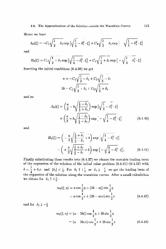
4.6. The Approximation of the Solution outside the Transition Curves 113
Hence we have
and
~0/~/= ~111 ~1 explll ~ ~1 +~11-~
~0~) ~il+~ex~ El I ~ ~l+~i~+~lexp E 1 4 ~1~ ~1 Inserting the initial conditions (6.4.38) we get
a - - C l l l - 51 -Jr- C 2 1 ~ - 51
2b= C l l l - + - 5 1 - t - C 2 ~ / 1 +51
and so
( a ~ exp [ - 512. ~] A 0 ( ~ ) - ~ - b 1 5 + 5 i
( ~ 1 51) i l + ~+ba 2z- e x p [ - - 5 2 . ~ ]
5 + 5 1
and
(6.4.40)
1 1 w0(~, ,/) = (a - 2b~) cos ~rl + 2bsin ~,/
1 1 = (a - 2b~z) cos ~ z + 2b sin ~ z (6.4.43)
1 and for 515 2
( j1 b>exp a ~ + 5 1 B0(~)= -~ ~ - ~ + [ -~.~]
( i 1 ) a g + 5 1 1 51 + b exp [ - _ 512 . ~c], (6.4.41) + +~ ~_
Finally substituting these results into (6.4.37) we obtain the unstable leading term of the expansion of the solution of the initial value problem (6.4.31)-(6.4.32) with
1 1 For 51 1"+1 1 5 = ~ -Jr- 51g and 151t < 2" ~ or 51 $ --5 we get the leading term of
the expansion of the solution along the transition curves. After a small calculation 1. we obtain for 51 1" +5
1 1 w0(~, rl) = a cos ~ r /+ (2b - a~) sin ~rl
1 1 = a c o s - z + ( 2 b - acz)sin-z (6.4.42)
2 2
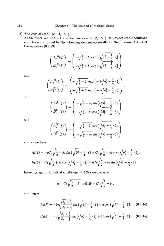
o o
..~
~176 I
Ii
"~
"~
~ ~
' "~
I I
~ ~
~ ~
'~
�9 ~ 0
0 .,~
o
~ I
+ l
I ""~
o o
.,-, ~
~~
,_,~.~
~ II
II II
~.~
~
~'0 ~
~ .~
,,,,~
~ ~
0
o c.,)
: r.
C C
+ ...,
~ II
�9 ~
r "I=I
~ ,
'-' 8
u
C
o o,i,
0 C9
0
'-0
.,d ,,d
.,,. ~
o o
o o
-l- 4-
.-.....:>
~I~ ,,~ ir162
q
I I
II II
o.../, .o,i,
o o
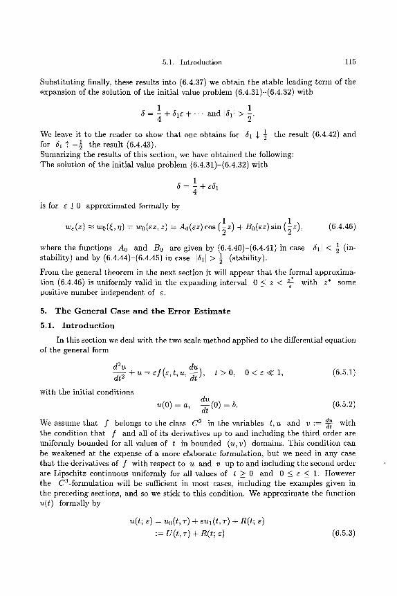
5.1. Introduction 115
Substituting finally, these results into (6.4.37) we obtain the stable leading term of the expansion of the solution of the initial value problem (6.4.31)-(6.4.32) with
1 1 5 - ~ + 51e + . . . and I~1 > ~.
1 the result (6.4.42) and We leave it to the reader to show that one obtains for 51 $ 1 the result (6.4.43). for 51 ~ ' - -~
Sumarizing the results of this section, we have obtained the following: The solution of the initial value problem (6.4.31)-(6.4.32) with
1 5 - ~ + e51
is for e $ 0 approximated formally by
1 l z ) , (6.4.46) w~(z) ,~ wo(~, 77) - Wo(eZ, z) = Ao(eZ) cos (~z) + Bo(ez) sin (~
1 (in- where the functions Ao and Bo are given by (6.4.40)-(6.4.41)in case ~11 < 1 (stability). stability) and by (6.4.44)-(6.4.45)in case 1511 >
From the general theorem in the next section it will appear that the formal approxima- z* Z* tion (6.4.46) is uniformly valid in the expanding interval 0 < z < -7- with some
positive number independent of e.
5. T h e G e n e r a l C a s e and t h e Error E s t i m a t e
5.1. I n t r o d u c t i o n
In this section we deal with the two scale method applied to the differential equation of the general form
d2u dt--- ~ + u = e f ( e , t , u , - ~ ) , t > 0 , 0 < e < < l , (6.5.1)
with the initial conditions du
u(O) -- a, -~-(0) -- b. (6.5.2)
d~ with We assume that f belongs to the class C 3 in the variables t, u and v "- -~- the condition that f and all of its derivatives up to and including the third order are uniformly bounded for all values of t in bounded (u, v) domains. This condition can be weakened at the expense of a more elaborate formulation, but we need in any case that the derivatives of f with respect to u and v up to and including the second order are Lipschitz continuous uniformly for all values of t _~ 0 and 0 _~ E _~ 1. However the 3 C -formulation will be sufficient in most cases, including the examples given in the preceding sections, and so we stick to this condition. We approximate the function u(t) formally by
u(t; e) = to( t , T) + Cit I (t, 7") d- R(t; e) := U(t, r)+ R(t; e) (6.5.3)
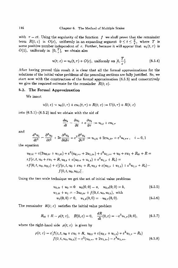
116 Chapter 6. The Method of Multiple Scales
with T -- et. Using the regularity of the function f we shall prove that the remainder T where T is term R(t; e) is O(e), uniformly in an expanding segment 0 < t < -/,
some positive number independent of e. Further, because it will appear that ut (t, ~-) is O(1) uniformly in [0, T , -/], we obtain also
u(t; e) = uo(t, ~') + O(e), uniformly on [0,--T]. (6.5.4)
After having proved this result it is clear that all the formal approximations for the solutions of the initial value problems of the preceding sections are fully justified. So, we start now with the construction of the formal approximation (6.5.3) and consecutively we give the required estimate for the remainder R(t; e).
5.2. T h e F o r m a l A p p r o x i m a t i o n
We insert
u(t; e) - uo(t, T) + eul (t, T) + R(t; e) := U(t, T) + n(t; e)
into (6.5.1)-(6.5.2) and we obtain with the aid of
and d2ui 02ui
dt 2 Ot 2 the equation
dui Oui igui dt Ot + e-O-TT := ui,t + eui
02Ui e2 02Ui + 2eo-~T + OT 2 "= Ui,tt "~- 2eui,t~ + e 2ui,Tr, i = 0 , 1
Uo,tt -~- ~(2UO,tT ~- Ul,tt) -~- E2(tt0,rT "~- 2Ul , t r ) "{- e3Ul,~-T -[- U0 -~- ~ttl -~- Rtt ~- R =
ef(e, t, Uo -+- eul + R, uo,t + e(uo,~ + ~tl,t) -{- ~2~tl,v -{- Rt) :
ef(0, t, Uo, Uo,t) + e[f (e, t, uo + eUl + R, uo,t + e(uo,r + Ul,t) + e2Ul,T ~- R t ) -
f (0 , t, ~0, ~0,,)].
Using the two scale technique we get the set of initial value problems
~o,,, + uo = o uo(O, o) = ~, ~o,,(o, o) = b,
Ul,tt + Ul = -2uo, t , + f(0, t, uo, uo,t), with
Ul(O, o) = o, Ul,,(o, o) = -~o,~(o, o).
(6.5.5)
(6.5.6)
The remainder R(t; e) satisfies the initial value problem
dR (0, e) = - e 2ul (0, 0), n . + R = p(t; ~), R(0, ~) = 0, ~ ,~
where the right-hand side p(t; e) is given by
p(t; e) = elf(e, t, uo + eUl + R, uo,t + e(uo,, + Ul,t) + e2Ul,r + nt)
- f ( 0 , t, ~0, ~o,,)] - ~ ( ~ 0 , ~ + 2~1,,~) - ~ , ~ .
(6.5.7)
(6.5.s)
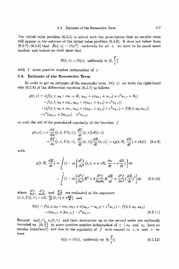
5.3. Estimate of the Remainder Term 117
The initial value problem (6.5.5) is solved with the prescription that no secular term will appear in the solution of the initial value problem (6.5.6). It does not follow from (6.5.7)-(6.5.8) that R(t; e) = O(e 2) uniformly for all t; we have to be much more modest, and indeed we shall show that
T R(t; e) = O(e), uniformly in [0, ~-]
with T some positive number independent of e.
5.3. E s t i m a t e of t h e R e m a i n d e r T e r m
In order to get an estimate of the remainder term R(t; e) we write the right-hand side (6.5.8) of the differential equation (6.5.7) as follows
p(t; -C) : c [ f ( c , t, U 0 -~- CUl -~- R , Uo, t n L ~(~t0, r n t- ~tl,t) -~- C2Ul,r -~ R t )
- f ( r t, Uo + CUl, ~to,t -~- C(Uo,r -1- Ul, t ) -1- g'2Ul,r)]
-~-~[f(~, t, It 0 -~- g'Ul, Zto, ̀ -~- c(Zto, r -~- Ul,t) -Jr g'2Ul,r) - f (O, t, Zto, Uo,t) ]
--C2(U0,1-T ~- 2Ul,t~-) -- e3Ul,r~-
or with the aid of the postulated regularity of the function f
Of dU (e, t, U(t, 7"), ~ (t, T))R(t; e) =
+-~vOf (e, t, U(t, T), dU_~ (t, T)) -d~dR (t; e)] + eg(t, R, --~dR) + eh(t)
with
(6.5.9)
1
g (t, R, --~) = (1 - s) -~fis2 (e, t, u + sR, -d-[ + s ---d~ ) ds 0
1
+ 2 + ( ds o
(6.5.10)
where o_~ ~ and ~ f Ou2, ouo, ~ are evaluated at the argument (e, t, U(t, T) + sR, ~dU (t, T) + S-x~)dR and
h(t) - f(e, t, uo + eUl, uo,t + e(uo,~ + Ul,t) + e2Ul,~) - f(O, t, uo, uo,t) -e (u0 , r r + 2Ul,tr) - e2Ul,~. (6.5.11)
Because u0(t, T), ul( t , T) and their derivatives up to the second order are uniformly bounded on [0, T] by some positive number independent of e (u0 and Ul have no secular behaviour!) and due to the regularity of f with respect to e, u and v we have
h(t) = O(e), uniformly on [0,--T]. (6.5.12)
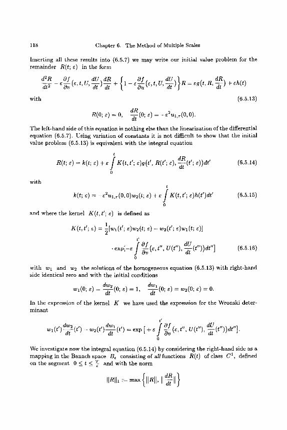
118 Chapter 6. The Method of Multiple Scales
Inserting all these results into (6.5.7) we may write our initial value problem for the remainder R(t; E) in the form
d2R Of dU dR { Of (~,t,u, dU } dR dt 2 e-~v(e,t,U,--~)-~+ 1-e-~u --~) R=eg(t ,R,--~)+eh(t)
with (6.5.13)
dR (0; e) = -e2ul,~(0, 0) n(0; ~) = o, ~
The left-hand side of this equation is nothing else than the linearization of the differential equation (6.5.7). Using variation of constants it is not difficult to show that the initial value problem (6.5.13) is equivalent with the integral equation
t
R(t; e) = k(t; e)+ e K(t,t'; e)g(t', R(t'; e),--~-(t'; e))dt' (6.5.14)
0
with t
k(t; ~) = -c2u1,~(0, 0)w2(t; ~) + e / K(t,t'; 6)h(t')dt' (6.5.15) a t 4
0
and where the kernel K(t,t'; e) is defined as
K(t, t'; e) = 1 ~[~(t'; ~)~(t; ~ ) - ~2(t'; ~)~(t; ~)]
�9 exp[-e f Ov0f (~, t" , V(t"), -~dU (t"))dt"] (6.5.16)
0
with wl and w2 the solutions of the homogeneous equation (6.5.13) with right-hand side identical zero and with the initial conditions
Wl(0; e) = dw2 (0; ~) = 1, dwl (0; e) = w2(0; E) : 0.
In the expression of the kernel K we have used the expression for the Wronski deter- minant
t ~
dw2 dwl f cg f (~, t", dU wl ( t ' )~ ( t ' ) - w2(t')--~-(t') = exp [ + e Ov U(t"), --~(t"))dt"]. 0
We investigate now the integral equation (6.5.14) by considering the right-hand side as a mapping in the Banach space B~ consisting of all functions R(t) of class C 1, defined on the segment 0 < t < T and with the norm
IIRIII :--max IIRII, II--~-II
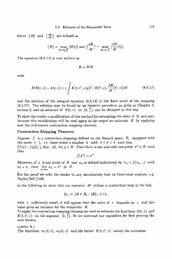
5.3. Estimate of the Remainder Term 119
where ][R][ and ]]dR [[ are defined as
dR IIR[I = max IR(t) l and [ l ~ l l
0 < t < T
dR -- max [--d-~-(t)[.
o<t<~
The equation (6.5.14) is now writ ten as
R = M R
with
t
f MR( t ; c) = k(t; ~) + c K( t , t'; e)g(t' , n(t ' ; ~),--~-(t';
0
(6.5.17)
and the solution of the integral equation (6.5.14) is the fixed point of the mapping (6.5.17). The solution may be found by an iterative procedure as given in Chapter 3, section 2, and an estimate of R(t; r on [0, T] can be obtained in this way.
To show the reader a modification of this method for est imating the order of R and also, because this modification will be used again in the sequel we estimate R by applying now the well-known contraction mapping theorem.
C o n t r a c t i o n M a p p i n g T h e o r e m
Suppose f is a contraction mapping defined on the Banach space B, equipped with the norm [[. [[, i.e. there exists a number k with 0 <_ k < 1 such that [ [ f ( x ) - f(y)[[ <_ k[[x-y[I , Vx, y E B. Then there is one and only one point x* C B such that
f (x*) = x*.
Moreover, i f x is any point of B and x , is defined inductively by x , = f ( x , - l ) with xo = x, then lim x,~ = x* in 17.
For the proof we refer the reader to any introductory text on functional analysis, e.g. Naylor/Sell [109].
In the following we show that our operator M defines a contraction map in the ball
Kr : : {R e B~ ; IIRII~ ~ r},
with r sufficiently small; it will appear that the value of r depends on r and this value gives an estimate for the remainder R. To apply the contraction mapping theorem we need to estimate the functions k(t; ~) and g ( t , t'; r on the segment [0, T]. So we interrupt our exposition for first proving the next lemma.
LEMMA 6.1 The functions Wl (t; ~), w2(t; 8) and the kernel g ( t , t'; ~) satisfy the estimates
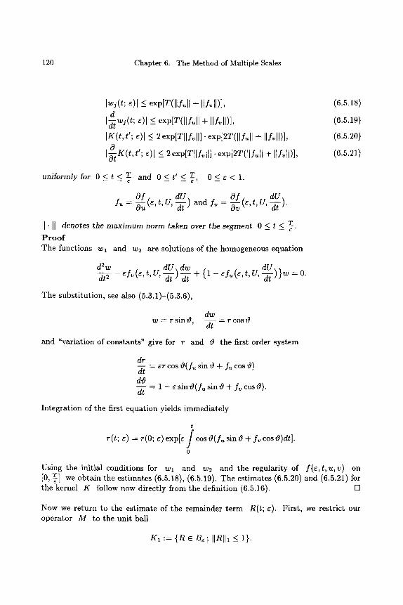
120 Chapter 6. The Method of Multiple Scales
Iwj(t; ~)1 <- exp[T(llf~,ll + IIL, II)],
[~wjd (t; e)l - < exp[T(llf~,ll + Ilfvll)],
[K(t,t'; E)[ < 2exp[TIIf~ll]" exp[2T(llf,,ll + IIL, II)],
1-~0 K(t,t'; e)[ <_ 2 exp[TIIf,,ll]" exp[2T(llf~,ll + IIf,,ll)],
(6.5.18)
(6.5.19) (6.5.20)
(6.5.21)
T 0 < ~ < 1 uniformly for O <_ t _< T~ and O _< t' _< -[, _ .
Of (e, t, U, dU Of (e, t, U, dU I~ = ~ 7?) ~ d I . - ~ ~).
[1-[1 denotes the m a x i m u m norm taken over the segment 0 < t < T_.
P r o o f The functions wl and w2 are solutions of the homogeneous equation
d2w dU dw dU dt--- 5- - e f , (e, t, U,--d-~)--d- ~ + {1 - e fu (e, t, u, --~ ) }w = o.
The substi tut ion, see also (5.3.1)-(5.3.6),
dw w = r sin 0, = r cos 0
dt
and "variation of constants" give for r and 0 the first order system
dr d--t = ~r cos tg(f,~ sin t9 + f~ cos O)
dO d---t- - - 1 - e s i n 0 ( f ~ , s i n z9 + fv cos 0).
Integrat ion of the first equation yields immediately
t
r(t; r = r(O; e) exp[r J cos tg(f~, sin 0 + f,, cos O)dt].
0
Using the initial conditions for Wl and w2 and the regulari ty of f(~, t, u, v) on T [0, ~-] we obtain the est imates (6.5.18), (6.5.19). The estimates (6.5.20) and (6.5.21) for
the kernel K follow now directly from the definition (6.5.16). []
Now we return to the est imate of the remainder te rm R(t; ~). First, we restrict our operator M to the unit ball
K1 "---- {R e B~ ;IIRII1 _ 1}.
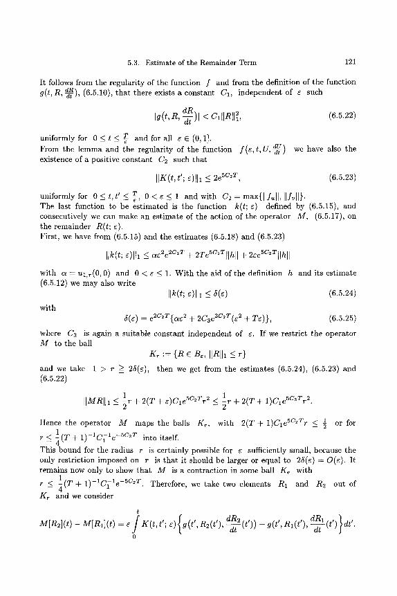
5.3. Estimate of the Remainder Term 121
It follows from the regulari ty of the function f and from the definition of the function g(t, R, ~tt), (6.5.10), tha t there exists a constant C1, independent of e such
dR [g (t, R, -~-)[ < C111RII~, (6.5.22)
T and for all e C (0, 1]. uniformly for 0 < t < -}-
From the l emma and the regulari ty of the function f (e , t , U, ~t) existence of a positive constant C2 such tha t
we have also the
IIK(t,t'; e)lll _< 2e 5c~T, (6.5.23)
T -- m~x{ l l f~ l l IIf~ll}" uniformly for 0 _ t , t ~_< ~-, 0 < e _ < 1 and with C2 The last function to be es t imated is the function k(t; e) defined by (6.5.15), and consecutively we can make an es t imate of the action of the opera tor M, (6.5.17), on the remainder R(t; e). First, we have from (6.5.15) and the est imates (6.5.18) and (6.5.23)
Ilk(t; ~)11~ <_ ~ 2 j c ~ , § 2T~SC.TIIhl I § 2e~SC.Tiihl I with a = ul,~(0, 0) and 0 < e _< 1. Wi th the aid of the definition h and its es t imate (6.5.12) we may also write
Ilk(t; e)ll~ _< 5(e) (6.5.24) with
5(e) = e 2c~T{~e 2 + 2C3e 3C"T (e 2 + Te)}, (6.5.25)
where C3 is again a suitable constant independent of c. If we restrict the opera tor M to the ball
K~ := {R e Be, IIRII1 < r}
and we take 1 > r => 26(e), then we get from the est imates (6.5.24), (6.5.23) and (6.5.22)
[[MR[]I < ~r + 2(T + r 2 < l r _ _ ~ + 2(T + 1)Cle5C~Tr 2
1 Hence the operator M maps the balls Kr , with 2(T + 1)ClehC~Tr <_ -~ or for 1 r < - (T + 1) - lC l le -5C2T into itself.
- 4 This bound for the radius r is certainly possible for e sufficiently small, because the only restr ict ion imposed on r is tha t it should be larger or equal to 25(e) = O(e). It remains now only to show tha t M is a contract ion in some ball K~ with
1 r _ < - ( T + 1) -1 -5C2T C~le . Therefore, we take two elements R1 and R2 out of 4
Kr and we consider
t
M[n2]( t ) - M[n~]( t ) - e K(t,t '; e) g(t',R2(t'), ~ ( t ' ) ) - g(t' ,Rl(t'), ~ ( t ' ) dr'. 0
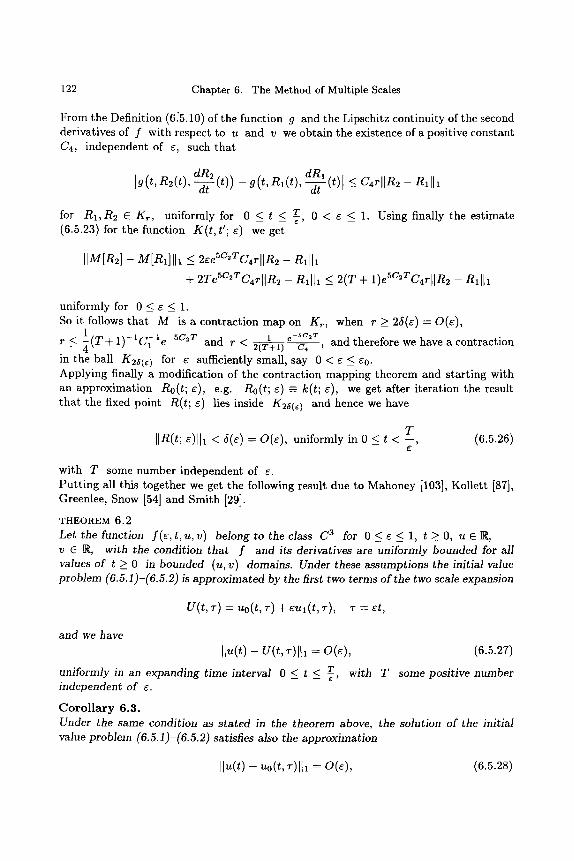
122 Chapter 6. The Method of Multiple Scales
From the Definition (6:5.10) of the function g and the Lipschitz continuity of the second derivatives of f with respect to u and v we obtain the existence of a positive constant C4, independent of e, such tha t
dR1 dR2 (t, n l (t) ~ _ Ig(t, R2(t), ~ ( t ) ) - g , (t) I < C4rllR2 - R~II~
T for R1,R2 C Kr, uniformly for 0 < t _ -/, 0 < e < 1. Using finally the est imate (6.5.23) for the function g ( t , t ' ; e) we get
IIM[R2]- M[R~]II~ <_ 2eeSC'TC4r l lR2 - n~ll l
+ 2TeSC~TC4rl lR2 - R~II~ _< 2(T + 1)ehC'TC4r l ln2 - R~II~
uniformly for 0 _ e _< 1. So it follows tha t M is a contraction map on g r , when r > 25(e) - O(e),
1 e--hC2T r < - (T + 1)- 1C~ 1 e-hC2T and r < 2(~+1) c4 and therefore we have a contraction
- - 4
in the ball K25(e ) for e sufficiently small, say 0 < e _< eo. Applying finally a modification of the contraction mapping theorem and s tar t ing with an approximat ion Ro(t; e), e.g. Ro(t; e) - k(t; e), we get after i terat ion the result tha t the fixed point R(t; e) lies inside K25(e) and hence we have
T IlR(t; ~)11~ < ~(~) = 0(~), uniformly in 0 _< t < --, (6.5.26)
with T some number independent of e. Pu t t ing all this together we get the following result due to Mahoney [103], Kollet t [87], Greenlee, Snow [54] and Smith [29].
THEOREM 6 . 2
Let the function f (e, t, u, v) belong to the class C 3 for O <_ e <_ 1, t >_ O, u E R, v E R, with the condition that f and its derivatives are uniformly bounded for all values of t >_ 0 in bounded (u, v) domains. Under these assumptions the initial value problem (6.5.1)-(6.5.2) is approximated by the first two terms of the two scale expansion
u ( t , ~) = uo( t , ~) + ~u~ (t, ~-), ~ = ~t,
and we have
II~(t) - u ( t , ~)11~ = o ( e ) , (6.5.27)
T with T some positive number uniformly in an expanding time interval 0 ~_ t ~_ -~, independent of e.
C o r o l l a r y 6.3. Under the same condition as stated in the theorem above, the solution of the initial value problem (6.5.1)-(6.5.2) satisfies also the approximation
Ilk(t) - u0(t, ~)11~ - 0 (~ ) , (6.5.28)
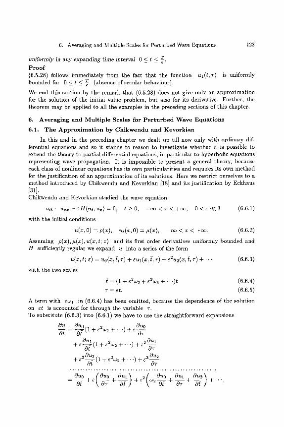
6. Averaging and Multiple Scales for Perturbed Wave Equations 123
uniformly in any expanding time interval 0 ~ t ~ T_.
P r o o f (6.5.28) follows immediately from the fact that the function ul(t , T) is uniformly
T (absence of secular behaviour). bounded for 0 _ t _< -/
We end this section by the remark that (6.5.28) does not give only an approximation for the solution of the initial value problem, but also for its derivative. Further, the theorem may be applied to all the examples in the preceding sections of this chapter.
6. A v e r a g i n g a n d M u l t i p l e Scales for P e r t u r b e d W a v e E q u a t i o n s
6.1. T h e A p p r o x i m a t i o n by C h i k w e n d u a n d K e v o r k i a n
In this and in the preceding chapter we dealt up till now only with ordinary dif- ferential equations and so it stands to reason to investigate whether it is possible to extend the theory to partial differential equations, in particular to hyperbolic equations representing wave propagation. It is impossible to present a general theory, because each class of nonlinear equations has its own particularities and requires its own method for the justification of an approximation of its solutions. Here we restrict ourselves to a method introduced by Chikwendu and Kevorkian [18] and its justification by Bckhaus [31]. Chikwendu and Kevorkian studied the wave equation
u t t - u x x + e H ( u t , u x ) = O , t_>0, - c x ~ < x < + c x ~ , 0 < ~ < < 1 (6.6.1)
with the initial conditions
u ( x , O ) - p(x), u t ( x ,O)= #(x), -cxD < x < +exp. (6.6.2)
Assuming p(x), It(x), u(x, t; ~) and its first order derivatives uniformly bounded ~nd H sufficiently regular we expand u into a series of the form
u(x, t; e) = uo(x, t, T) + ~U 1 (X, t, T)-~- e2U2(X, t', T) -[- �9 �9 �9 (6.6.3)
with the two scales
t '-- (1 + e2w2 + e3w3 + . . . ) t (6.6.4)
7 = et. (6.6.5)
A term with. r in (6.6.4) has been omitted, because the dependence of the solution on et is accounted for through the variable ~-. To substitute (6.6.3) into (6.6.1) we have to use the straightforward expansions
Duo O__U_U _ Ouo (1 + e2w2 + . . - ) + e 0T o t - o~
OU 1 (1 + e2 W~ + ' ' ' ) + e~ OU 1 + ~ - j Or
+ E20u2 (1 + e2w2 + . . . ) + e30u2 - - j o7-
. . . . . . . . . . . . . . . . . . . . . . . . . . . . . . . . . . . . . . . . . . . . . . . . . . . . . . . . .
__ OUo . / OUo OQUl ~ 2 / OUo (~Ul OU2 -~ e + + e w2 + + + ."
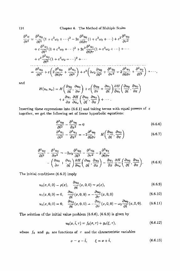
124 Chapter 6. The Method of Multiple Scales
02u Ot 2
_ 02 02U~ (l + e2w2 + .)~ 02U~ (l + e2w2 + . ..) + e2 u0 - 0{ 2 .. + 2 e ~ 0T 2
02Ul (1 + e2w2 + )2 02Ul + e - - - ~ . . . + 2 e 2 0 - - - ~ T ( l + e 2 w 2 + . . - ) + ' "
202u2(1 +e2w2 + .)2 + e - ~ .- + . . .
02uo . {- 02uo O~ul'~ 2 {- Ouo O~uo O~ul 02u2 : ~ *~[~o3~ + - ~ ) + ~ [ 2 ~ ~ + - ~ +2o-~ + o~ ] + '
and (o.oouo) iouoo..)o.(o oouo) H(ut, u x ) = H Or' Ox + e \ OT +---~ ~ Or' Ox
Oul OH ( Ouo Ouo ) + ~ o---~ ou----: \ o~ ' o~ + "
Inserting these expressions into (6.6.1) and taking terms with equal powers of e together, we get the following set of linear hyperbolic equations:
02uo 02uo 0{2 Ox2
02ul 02ul 0{2 Ox 2
- -0
= _ 2 0 2 u 0 - H(OUo Ouo) ot~r o~' o~
(6.6.6)
(6.6.7)
02u2 o ~
02u2 02uo 02uo 02ul -- - - 2 w 2 - - 2 _ Ox 2 O~ 2 Ov 2 OtOv (ouo ouo) o.(o.o o.o)
- ~ + o ~ l ~ o ~ ' o ~ o~ o~,~ o ~ ' o ~ "
The initial conditions (6.6.2) imply
Ouo (~, o, o) = #(~), uo(~, o, o) = p(~), - - ~
Ou 1 Ouo ( x, 0, 0) u~ (~, o, o) = o, -g~-(~, o, o) = - - g ; (
Ou2 Oul Ouo (x, O, O) ~,~(~,o,o) = o, - -~ (~ , o, o) = - - g ; ( ( ~ , o, o) - ~ - ~
The solution of the initial value problem (6.6.6), (6.6.9) is given by
uo(~, ~, ~) = f0(o, ~) + go(~, ~),
where f0 and g0 are functions of ~- and the characteristic variables
(6.6.8)
(6.6.0)
(6.6.10)
(6.6.11)
(6.6.12)
a - - x - - t , ~ -- x-k- t, (6.6.13)
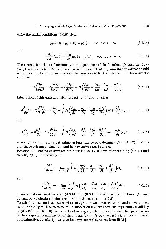
6. Averaging and Multiple Scales for Perturbed Wave Equations 125
while the initial conditions (6.6.9) yield
f0(~, 0)+ 90(~, 0)= o(~), - ~ < �9 < + ~ (6.6.14)
and Ogo -Ofo (x 0) + (x, 0) #(x) - o c < x < +cx). (6.6.15)
0~ ' - - ~
These conditions do not determine the T dependence of the functions" fo and go; how- ever, these are to be obtained from the requirement that Ul and its derivatives should be bounded. Therefore, we consider the equation (6.6.7) which reads in characteristic variables
02u: 02fo 029o (09o Ofo 09o Ofo'~ (6.6.16) --4 00.O~ -- 2 00.OT -- 20~oT -- H --~ Oa ' O~ + M ]"
Integration of this equation with respect to ~ and a gives
OUl 02 fO 209of ( Ogo O fo Ogo O fo ~. O f l -4- -0~ a = 2~ - - H ~ + d~ + (a, T) (6.6.17)
and
o" .u: 0..o / (0.o -4-0-~ - 2 - 2Oo~oT - H 0,~
O fo Ogo O fo ) Ogl Oa ' 0---( + -~a da + - -~(~ , T) (6.6.18)
where f : and g: are as yet unknown functions to be determined from (6.6.7), (6.6.10) and the requirement that u2 and its derivatives are bounded. Because u: and its derivatives are bounded we must have after dividing (6.6.17) and (6.6.18) by ~ respectively a
02fO if (Ogo Ofo Ogo Ofo'~ 2 ~ = lim H ~ + d~, (6.6.19) o~o~ ~ - ~ o~ o~ ' o~ ~ )
and o"
,.,0 , / ( , , 0 ,,0 ,,0 20~0----- ~ = - l i m - H o ~ a O~ Oa O~ + ~ ] da. (6.6.20)
These equations together with (6.6.14) and (6.6.15) determine the functions f0 and go and so we obtain the first term u0 of the expansion (6.6.3). To calculate f0 and go we need an integration with respect to T and so we are led to an averaging with respect to T. In subsection 6.3. we show the approximate validity of (6.6.19) and (6.6.20) by using local averaging. Before dealing with the justification of these equations and the proof that uo(x, t, T) = fO(a, 7") + go(~, T), is indeed a good approximation of u(x, t), we give first two examples, taken from lit[18].
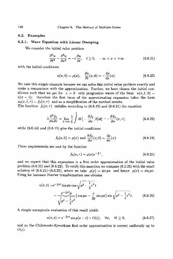
126 Chapter 6. The Method of Multiple Scales
6.2. E x a m p l e s
6.2.1. W a v e E q u a t i o n w i t h L inea r D a m p i n g
We consider the initial value problem
02u 02u Ou O t 2 O x 2 = - e - i f i , t >>_ O,
with the initial conditions
-o0 < x < +c~ (6.6.21)
Ou dp u(x,O) = p(x), -~-(x, 0) = -~xx(X). (6.6.22)
We take this simple example because we can solve this initial value problem exactly and make a comparison with the approximation. Further, we have chosen the initial con- ditions such that we get for e = 0 only progressive waves of the form u(x, t; O) = f i ( x - t); therefore the first term of the approximating expansion takes the form uo(x, t, T) = fo(a, T) and so a simplification of the method results. The function fo(a, T) satisfies according to (6.6.19) and (6.6.21) the equation
02f0 = lim 1 - - J H ( _ O f o O)d~= Ofo
~ ~ ~o ~ - f f j ' - - f f - j ( ~ ' ~ ) '
while (6.6.14) and (6.6.15) give the initial conditions
Ofo (a, O) = dp fo(a, O)= p(a) and ~ ~--~a (a).
These requirements are met by the function
f0(~, ~) = p(o)~-�89
(6.6.23)
(6.6.24)
(6.6.25)
and we expect that this expression is a first order approximation of the initial value problem (6.6.21) and (6.6.22). To verify this assertion we compare (6.2.25) with the exact solution of (6.6.21)-(6.6.22), where we take p(x) = sinpx and hence p(a) = sinpa. Using for instance Fourier transformation one obtains
u(x, t) =e-�89 sinpx cos ~p2 - ~e2 t
e- �89 et p e ~/p - ( cospx - k sinpx) sin 2 _ 162 t.
Ip 2 _ 162 2io 4 4
A simple asymptotic evaluation of this result yields
u(x,t) = e-�89 ~t sinp(x - t) + 0(6), Vx, Vt >_ O,
(6.6.26)
(6.6.27)
and so the Chikwendu-Kevorkian first order approximation is correct uniformly up to o(~).
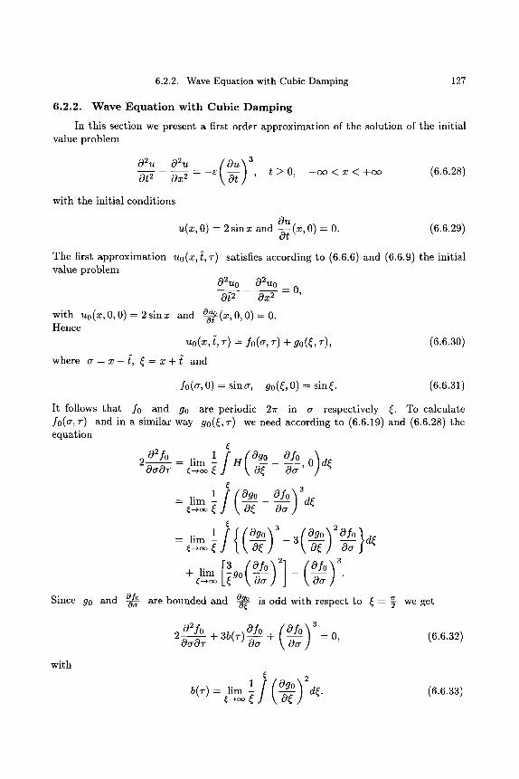
6.2.2. Wave Equation with Cubic Damping 127
6.2.2. Wave Equation with Cubic Damping
In this section we present a first order approximation of the solution of the initial value problem
G~2U 02~t / 0 U ) 3 Ot 2 Ox 2 = --e -~ , t > 0, --cr < x < +cr (6.6.28)
with the initial conditions
C~U u(x, 0) = 2s inx and - ~ ( x , 0) = 0. (6.6.29)
The first approximation uo(x, t, T) satisfies according to (6.6.6) and (6.6.9) the initial value problem
02uo 02uo O~ 2 Ox 2 = O,
with uo(x, 0, 0) = 2 sin x and - ~ (x, 0, 0) = 0. Hence
~o(~, ~, ~) = fo(~, ~) + go(~, ~), (~.6.3o) where a = x - t , ~ = x + t and
fo(a, O) = sin a, go(~, O) = sin~. (6.6.31)
It follows that f0 and go are periodic 21r in a respectively ~c. To calculate fo(a, T) and in a similar way g0(~ c, T) we need according to (6.6.19) and (6.6.28) the equation
202f~ = lim 1 / ( Ogo Ofo ) OaOT ~o~ ~ H O~ On' 0 d~
:,im 1/(o o o,o)
= lim l f { ( 0 g ~ 3 (Og~176 ~-+~ -0~-] - 3 \ 0~ ] ~-~
+ l i m ~ g o ( O f ~ 1 7 6 3 ~-+~ \ o~ \~-J
Since go and Ofo are bounded and o90 W( is odd with respect to ~ = y we get
with
O~fo Ofo (Ofo) ~ 2 o - j ~ ~ + 3b(~) + = o, (6.6.32)
'~ 2 (6.6.33)
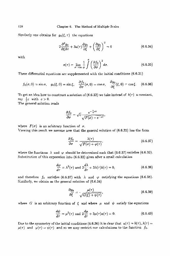
128 Chapter 6. The Method of Multiple Scales
Similarly one obtains for g0(~, r) the equations
02go Ogo logo ~ ~ 20~OT + 3a ( r ) + ] = 0 (6.6.34)
with
aim o - ~ ~ ~ do. (6.6.35)
These differential equations are supplemented with the initial conditions (6.6.31)
Ogo Ofo (a, 0) = cos a, (~c, 0) = cos ~. (6.6.36) fo(a, O) = sin a, g 0 ( ~ , 0 ) = s i n ~ , ~ - - ~
To get an idea how to construct a solution of (6.6.32) we take instead of b(r) a constant, 1 say 5c with c > 0 .
The general solution reads
0o v/F(o) - ~-~;'
where F(a) is an arbitrary function of a. Viewing this result we assume now that the general solution of (6.6.32) has the form
0fo = )~(r) (6.6.37) 0o v~F(~) + r162
where the functions A and qa should be determined such that (6.6.37) satisfies (6.6.32). Substi tution of this expression into (6.6.32) gives after a small calculation
dqo = A2 (r) and 2 d)~ dr -~r + 3A(r)b(r) = 0, (6.6.38)
and therefore f0 satisfies (6.6.37) with A and qo satisfying the equations (6.6.38). Similarly, we obtain as the general solution of (6.6.34)
Ogo = #(r) (6.6.39) 0r ~/a(r + r162
where G is an arbitrary function of ~ and where # and r satisfy the equations
de = #2(r ) and 2 du dT d r + 3#(T)a(T) = O. (6.6.40)
Due to the symmetry of the initial conditions (6.6.36) it is clear that a( r ) -- b(r), A(T) = #(T) and ~a(r) = r and so we may restrict our calculations to the function f0.
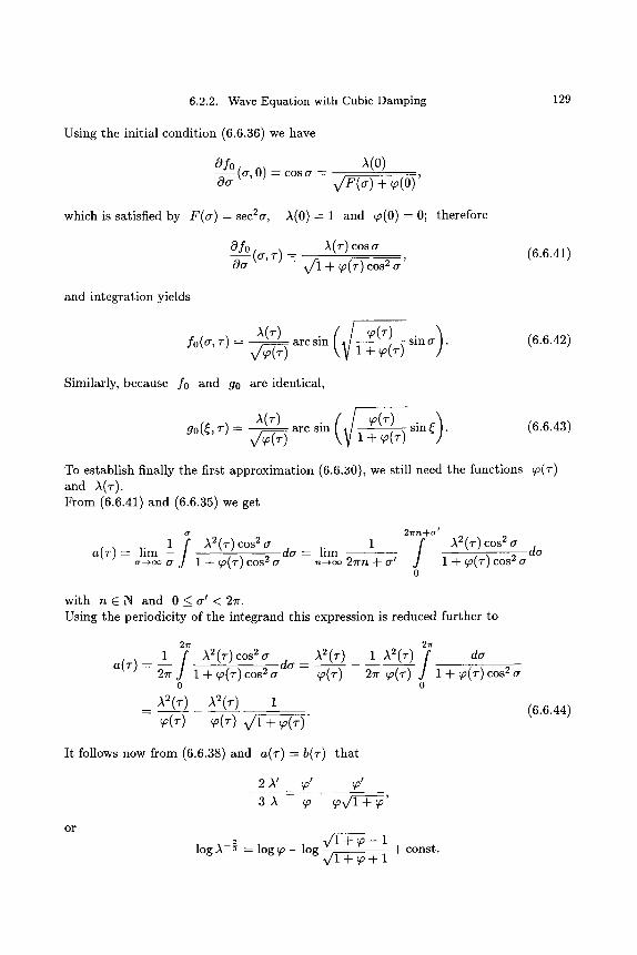
6.2.2. Wave Equation with Cubic Damping 129
Using the initial condition (6.6.36) we have
~(0) Ofo (a, 0) = cos a = 0~ v/F(~) + ~(0)
which is satisfied by F(a) - sec2a, A(0) = 1 and ~(0) - 0; therefore
o f 0 (~,.) = ~ ( . ) cos
0a V/1 + ~(T)cos 2 a (6.6.41)
and integration yields
fo(a ,T)= A(T) ( i ~ ( T ) / (6.6.42) arc sin ~ sin a . (T) 1 + ~(T)
Similarly, because f0 and go are identical,
s i n ~ / �9 gO(~, T) -- arc sin \ Y l + ~(T--------)
To establish finally the first approximation (6.6.50), we still need the functions ~(T) and A(T). From (6.6.41) and (6.6.35)we get
a
a(T) = lim -if o ~ a 1 + ~(T) cos 2 a
2 7r I i ~I- o - I
do" = lim 1 f A2(T) cos 2 a do , ~ 2rn + a' 1 + ~(T) cos 2 a
0
with n C N and O < a ~<2Ir. Using the periodicity of the integrand this expression is reduced further to
271- 1 / A2(T) cos 2a
a(T) -- ~ 1 + ~(T)COS 2 a 0
A2(~ -) A2(T) 1
d o =
~(r) ~(r) V/1 + ~(r)"
271" A2(T) 1 A2(T) / da ~p(T) 2~- ~(7-) 1 + ~(T)COS 2 a
0
(6.6.44)
It follows now from (6.6.38) and a(T) -- b(T) that
3 ~ ~ ~ l V T ~ '
or X / I + w - - 1
log A-} = log ~ -- log V~ ~ ~ + 1 + const.
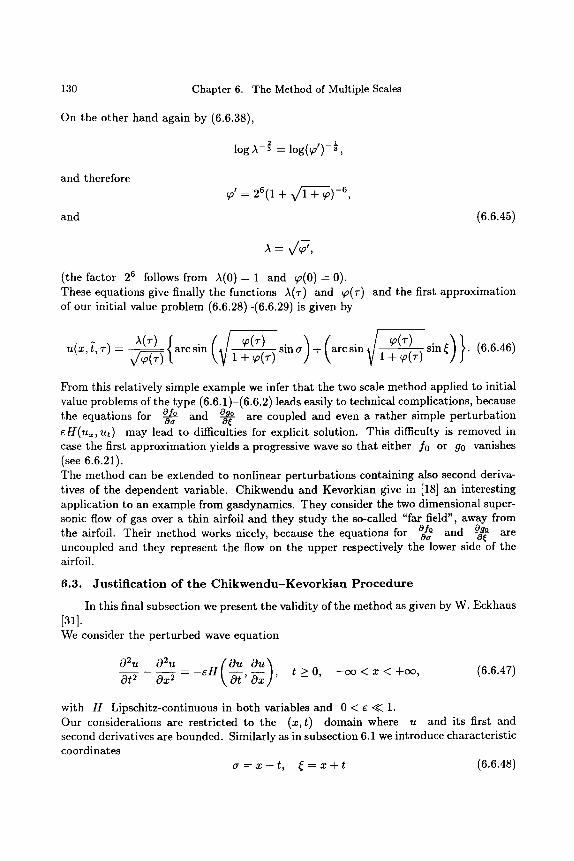
130 Chapter 6. The Method of Multiple Scales
On the other hand again by (6.6.38),
1
log A-] = log(~o')-g,
and therefore ~o'= 26(1 + V/1 + ~ ) - 6
and (6.6.45)
A= V/~,
(the factor 26 follows from A(0 ) - 1 and ~0(0)-0). These equations give finally the functions A(T) and ~o(~-) and the first approximation of our initial value problem (6.6.28)-(6.6.29)is given by
{ ( i ) ( i ~~ s in~)}" (6"6"46) u(x, t, T) -- X/~A(T) arc sin 1 +~0(T------~)~0(r) sin a + arcsin ~ 1 + ~O(T)
From this relatively simple example we infer that the two scale method applied to initial value problems of the type (6.6.1)-(6.6.2) leads easily to technical complications, because the equations for ~ and ~ are coupled and even a rather simple perturbation EH(ux, ut) may lead to difficulties for explicit solution. This difficulty is removed in case the first approximation yields a progressive wave so that either f0 or go vanishes (see 6.6.21). The method can be extended to nonlinear perturbations containing also second deriva- tives of the dependent variable. Chikwendu and Kevorkian give in [18] an interesting application to an example from gasdynamics. They consider the two dimensional super- sonic flow of gas over a thin airfoil and they study the so-called "far field", away from the airfoil. Their method works nicely, because the equations for ~ and ~ are uncoupled and they represent the flow on the upper respectively the lower side of the airfoil.
6.3. Jus t i f ica t ion of the C h i k w e n d u - K e v o r k i a n P r o c e d u r e
In this final subsection we present the validity of the method as given by W. Eckhaus [31]. We consider the perturbed wave equation
02u 02u (Ou Ou) Ot 2 Ox 2 = - e l l -~'-~x ' t >_ 0, -c~ < x < +c~, (6.6.47)
with H Lipschitz-continuous in both variables and 0 < e << 1. Our considerations are restricted to the (x,t) domain where u and its first and second derivatives are bounded. Similarly as in subsection 6.1 we introduce characteristic coordinates
a = x - t , ~ = x + t (6.6.48)
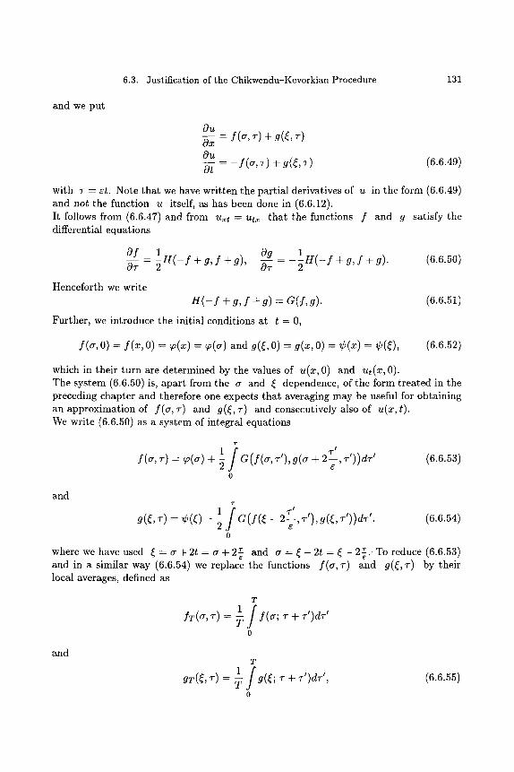
6.3. Justification of the Chikwendu-Kevorkian Procedure 131
and we put
~ u
0--x -- f(cr, T) + g(~, T)
OU cot = --f(0~, 7) + g(~C, 7-) (6.6.49)
with T -- et. Note that we have wri t ten the partial derivatives of u in the form (6.6.49) and not the function u itself, as has been done in (6.6.12). It follows from (6.6.47) and from u~t = ut~ tha t the functions f and g satisfy the differential equations
Of ] 0_~g = - H ( - f + g , f + g ) 0~" 2 ' OT
1 2 H ( - f + g, f + g). (6.6.50)
Henceforth we write
H ( - f + g, f + g) = G(f , g).
Further, we introduce the initial conditions at t = O,
(6.6.51)
f (a , O) = f (x , 0) = ~(x) = ~(a) and g(~, 0) - g(x, 0) = r -- r (6.6.52)
which in their turn are determined by the values of u(x, 0) and ut(x, 0). The system (6.6.50) is, apar t from the a and ~c dependence, of the form t reated in the preceding chapter and therefore one expects tha t averaging may be useful for obtaining an approximation of f (a , T) and g(~, 7-) and consecutively also of u(x, t). We write (6.6.50) as a system of integral equations
1 ] ~' f (a , 7") = qo(o) + -~ G( f (a , T'),g(a + 2--,e r'))dT'
0
(6.6.53)
and T
1 f T' g(~, ~) = r - ~ G(f(~ - 2-- , ~'), g(~, ~'))d~'. 0
(6.6.54)
To reduce (6.6.53) and a = ~ - 2 t = ~ - 2 7 where we have used ~ = a + 2 t = a + 2 7 and in a similar way (6.6.54) we replace the functions f (a , T) and g(~, T) by their local averages, defined as
and
T
if f~(,~, ~-) = ~ f(,~; ~- + ~-')d~-' 0
T 1/ ar(~, ~) = y a(~; ~ + ~')d~',
o
(6.6.55)
132 Chapter 6. The Method of Multiple Scales
see (5.2.11). Taking this average of f(a, T) we get from (6.6.53)
T r+~-'
1: {i .,, ) :T(a, T) = :(a) + ~ dT' a ( f (a , T'), g(a + 2--,e T"))dT" o 0
T T W r ' 1/ {/ T" } = ~,(.)+ ~ e~-' a(.:(., ~-"), g(. + 2--,~ ~-"))e~-"
0 I" ~
T "I" ~
1: {i ) -4- -~ dT' G(f(a, T"), g(a + 2--Z, )dT" 0 0
T r + v '
1i (i .,, } = r + ~ dT' a ( f (a , T"), g(a + 2--,e T"))dT" 0 1" ~
+ {O(T)}I.
The estimate {O(T)}t follows from the assumption that f and g are bounded and TIe
so also G(f(a, T"), g(a A- -7-, T")) Reducing :T(a, T) further we have
1 i { 2(T" T ' T " T'))dT" I t (o , ~-) = ~o(o) + ~ a~-' a(f(~, , ~-" + T'), g(~ + -~ + ), + 0 0
+ {O(T)}I
]{] ) 1 dr" r" 2 (r" r" = ~(a) + ~ G(f(a, + T'), g(a + -e + ~'')' + T'))dT' 0 0
+{O(T)) I "i" T
1 d r" -4- T') gT e = ~o(o1 + -~ a(Ir(o,~-" , (~, + - + 1, + o 0
+ {O(T)}I + {O(T)}2,
uniformly for finite values of T -- et, where we have used the Lipschitz-condition of G and Lemma 1 from Chapter 5, stating that for a uniformly Lipschitz continuous function f (t)
f(t) = fT(t) + O(T).
Inspecting the T-dependence of both order terms we may safely differentiate with respect to T and we get the initial value problem
T
CgfT(a,r ) = 1 i T' 2 0---7 ~ C(fT(a, T + ),gT(a + -('re + T'), T + T'))dT' + O(T) o
6.3. Justification of the Chikwendu4Kevorkian Procedure 133
with fT(o, O) ~ f (a, O) § O(T) ---- ~(a) + O(T). (6.6.56)
Because T ~ runs from 0 to T and because T is small we may write this equation a l s o as
T
OfT 1 i 2 -~f (a, T) ~. -j--~ G(fT(a, 7"), gT(o" + -('re + "P), T))dT' + O(T) 0
T
0
~+ aT
~4T i G(ST(a,'r), gT(~', T))d~' + O(T).
We suppose now that the initial values u(x, O) and ut(x, O) are periodic, with period independent of e, then also f(cr, T) and g(~, T) are periodic in a and ~ respectively, say with period w. Taking e - o(T), putt ing ~ = nw+5 with 0 ~ 5 < w, n E N, and using the periodicity of 9T(~ ~, z) we get
~w 1 { / 0~ (~' ~) = 2 ( ~ + ~) G(fr(~, ~), gr(~', ~))d~'
0
~+nw+5
+ f noJ
0
o r
OfT (cr, ~-) -- 1 lim 1 i e OT -~ ~ ~ G(fT(a, T), gT(~', T))d~' + 0(-~) + O(T). o
In quite a similar way one obtains also
o"
i OgTOT ((' T) = -- 2 ~--~o~1 lim la G(fT(a', T), gT(~, T))da' + 0 (~ ) + O(T). 0
An optimal choice for T is now given by T - O(v/~) and we have finally obtained the result
O f T ( a , T) --- 1 lim 1 f OT 5 ~---,~ ~ G(ST(U, "r), gT(~', r))d~' + R1 (6.6.57)
o
134 Chapter 6. The Method of Multiple Scales
and O
OgTOT (~C, T) = _12 a-~o~lim la J G(fT(a', T), gT(~, T))da' + R2 (6.6.58)
o
with R1 = O(x/~) and R2 = O(v~) and the initial conditions
fT(a, O) = r + O(T) : ~o(a) + O(yr-c)
and (6.6.59)
gT(,~, 0) = r + O(T) = r + O(v~).
In case the solution of these initial value problems depends continuously on the order terms O(x/~ ) in the vicinity of zero, one obtains a good approximation of the functions fT(a, "r) and gT(~, T) and thus also of f(a, "r) and g(~, r) by solving the initial value problems
Of (o, T) = 1 1 /
o
1 1/ = -~ ~fim ~ H( - ](a, "r) + [7(~', T), ](a, T) + 0('~', "r))d~', (6.6.60)
o
with f(a, 0) = ~(a), and
lim 1 ] G(](a', T), ~(~, T))da' O~ 1 o~- (~' ~) = --~ ~ -j
o
_- 1 lim _1 ~f H( - ](a', T) + ~(~, r), ](a', T) + ~(~, T))da', (6.6.61) 2 a--,~ a o . i
o
with .~((, 0) = r The continuous dependence of the solution of the initial value problems (6.6.57), (6.6.58) and (6.6.59) depends on the function H and this continuity should be checked for every given problem. When we replace in the initial value problems (6.6.60) and (6.6.61) the functions f and ~ by ~ respectively ~ we get the same equations as given by Chikwendu and Kevorkian and presented in the formulae (6.6.19) and (6.6.20). Therefore,
0/0 (~, ~) = ](~, ~) ~/(~, ~) Oa
and Ogo o~ (~' ") = ~(~' '9 ~ g(~, ~).
It follows that the solutions ~ - o90 and o~ of the equations (6.6.19) and (6.6.20) yield the functions f and g within the required accuracy and this justifies the Chikwendu and Kevorkian approach in the case that f(a, "r) and g(~, ~-) are periodic in a respectively
Exercises 135
The success of the multiple scale method has promoted the use of first order models for the description of several physical phenomena. Apart from the examples given before we mention here also the Korteweg-de Vries equation for long waves in a channel [94], [58] and the nonlinear SchrSdinger equation for the amplitude of modulated waves, [25], [58]. These examples have been a topic during the last twenty years in pure and applied research concerning the theory of solitons.
Exerc i se s
1. Give by using two time scales a first order approximation of the solution of the free van der Pol equation
du d2u (1 u2)-d- ~- d t--- ~ + u = r -
t > 0
with du
u(0) = cr > 0 and - ~ - ( 0 ) - 0.
2. Give by using two time scales a first order approximation of the solution of the initial value problem
d2u dt 2
du + u = 0 , t > 0
with du
u(0) = a and -~(0) = 0.
3. Give by using two time scales a first order approximation of the forced van der Pol equation
d2u du dt-- $ + w21u = r - u 2) --~ + 3" cos w2t
with du
u ( O ) = a , - ~ - ( O ) = O a n d w 2 - w l = O ( 1 ) ,
no resonance). Consider the following two cases: 3' is a constant with 3" = eft and 3" = O(1). See also [108, 6.2.3].

This Page Intentionally Left Blank
Chapter 7
S I N G U L A R P E R T U R B A T I O N S O F L I N E A R O R D I N A R Y D I F F E R E N T I A L E Q U A T I O N S
1. T h e Ini t ia l Va lue P r o b l e m
1.1. I n t r o d u c t i o n
In this section we construct an asymptot ic approximatio~ of the solution of the initial value problem
d2ue due Le[ue] = ~ ~ + a(x) ~ + b(x)ue - f(x), x > 0, (7.1.1)
with 0 < r ~ 1 and the initial conditions
due ue(0) - a, --~-x (0) - p, (7.1.2)
where c~ and ~ are a rb i t ra ry constants independent of ~. The coefficients a and b and the r ight-hand side f are submi t ted to the condition tha t they should belong to the space C~[0, c~) (continuously differentiable for 0 _< x < c~) and moreover tha t
a(x)_>ao>O, x > 0 , (7.1.3)
with a0 a constant independent of c. The la t ter condition is very essential because o t h e r w i s e - as will appear l a t e r - the construct ion breaks down. First we construct in subsection 1.2 a formal approximation of ue, i.e. an approximat ion tha t satisfies the differential equat ion and the initial conditions up to some order of ~. Consecutively we show in the next subsection 1.3 the validity of this formal approximation; the proof consists in an a priori es t imate of the error.
1.2. T h e Formal A p p r o x i m a t i o n
We expect tha t the solution ue will be approximated to some extent by the solution w of the reduced problem with ~ = 0. So we consider the initial value problem
a(x) dw + b(~)~ = f(~), (7.1.4)
138 Chapter 7. Singular Perturbations of Linear Ordinary Differential Equations
with w(0) = a. The solution reads
where
f ( ~ ) d , W(X)-- eq(X){o~2r- e-q(')~(~) ~} 0
(7.1.5)
y b(~) d~ q(x) = - ~ ~.
0
However this function does not satisfy in general the second initial condition (7.1.2) and so we need a correction term tha t accounts for this lost second boundary condition. Therefore we investigate the differential operator L~ in the neighbourhood of the point x = 0 more closely by using a "microscope" defined with the aid of the t ransformation
x = r v > 0. (7.1.6)
The operator L~ expressed in the new coordinate ~ is
d 2 d L~ = ~ 1 - 2 ~ , . +~-~a(~V~) . +b(~,~).
1 and to get a proper balance The most dominant terms are the first two whenever v > between these terms we put v = 1. Using now the supposed regularity of the coefficients a and b we have
L~ = E - I ~ _ 1 + ~0, (7.1.7)
with
and
d 2 d s = -7~,- +a(0)-7; ",
d f~o = ~--dx (zgE~)-~-~ . +b(e~) ., 0 < ~ < 1.
To satisfy both initial conditions at x -- 0 and the differential equation up to some positive order of e we make the following a t t empt for the formal approximat ion of uE:
u,(~) = ~(~) + ~(~-) + R,(~) = ~ ( ~ ) + , ( ~ ) + R,(~), (7.1.s)
where the correction term v(() satisfies the boundary walue problem
~_1 IV]----0, (7.1.9)
with the boundary conditions
dv 1 dv dw dx (O) = -~-~(0) - ~ - -~-~x (O),
1.2. The Formal Approximation 139
and (7.1.10)
lim v(~) = O. ~-+oo
The latter condition stems from the consideration that we want to represent the correc- tion term v(~) as a boundary layer term, that has for r $ 0 only significant values in a right small neighbourhood of x - 0. It follows immediately from (7.1.9) and (7.1.10) that v(~) is given by
dlu ~ ( o ) - Z v(~) = r a(O) exp [ - a(O)~-]. (7.1.11)
Putt ing w and v together we get
x d2w Le[w(x) + v ( ~ ) ] - f ( x ) + r + C0[v( )]
d2w da dv = f(x) + ~-j-fi~2 + r162162 + b(~r (7.1.12)
with
and
~'(o) - w(o) + v(o) - ~ + ~ ~ a ( 0 )
dw dv dx (0)+ -~x (O) = ~.
Because the data of our initial value problem (7.1.1)-(7.1.2) are C1[0, cr it follows from (7.1.5) and (7.1.11) that the right-hand side of (7.1.12) is f ( x ) + O ( ~ ) , uniformly in any bounded segment [0,~] with I positive and independent of ~, (n.b. ~exp[-a(0)~] is uniformly bounded in [0, co) ). So w ( x ) + v(~) is a formal approximation of ue in [0, ~]. We call this composite expression a formal approximation, because it satisfies the differential equation and the initial conditions up to O(~), uniformly in [0, ~]. Finally to show that w ( x ) + v(-~) is indeed a good approximation we consider the remainder term Re(x) defined in (7.1.8). It satisfies the initial value problem
d2w da dv Le[Re] = Le[ue - w - v] = -6-~fix2 - ~-~x (O~)--~ - b(r
= O(~), uniformly in [0, ~], (7.1.13)
with the initial conditions
dRe Re(O) = -v(O) = 0(r and -~-x (0) - 0. (7.1.14)
Given this initial value problem it is possible to derive an a priori estimate of Re(x) with- out solving explicitly the initial value problem (7.1.13)-(7.1.14). This a priori estimate is constructed in the next subsection and it will appear that Re(x) = 0(r uniformly in any bounded segment [0, g].
140 Chapter 7. Singular Perturbations of Linear Ordinary Differential Equations
1.3. T h e A P r i o r i E s t i m a t e o f t h e S o l u t i o n of a S i n g u l a r l y P e r t u r b e d O r d i n a r y D i f f e r e n t i a l E q u a t i o n w i t h G i v e n In i t i a l D a t a
We consider the initial value problem
d2u du ~ x 2 + a(x; ~)-~x + b(x; ~ ) u - f (x ; e) 0 < x < oo, (7.1.15)
with the initial conditionS
du u(O) = a(6), ~x(O) = 13(6). (7.1.16)
The coefficients a, b and the right-hand side f depend as well on x as on 6 and we assume that for .E sufficiently small a(x; E) is continuously differentiable with respect to x and that b(x; e) and f ( x , e ) are continuous in x for x _> 0. Moreover, there exist positive constants A , B and i, independent of E, such that
[a(x; 6)[ + [dxxda(x; 6)[ < A, ]b(x; E)[ < B, for 0 _< x _< l, (7.1.17)
uniformly for 6 sufficiently small, say 0 <. 6 < 60, where e0 will be used henceforth as a generic constant; this means that the value of e0 may be lowered in the sequel without violating earlier results. Further we assume that also the initial values a(6) and fl(r are bounded in [0, e0]. Finally, we make the crucial assumption
a(x; r _ ao > O, f o r 0 < x < g a n d 0 _ 6 < 6 0 , (7.1.18)
where a0 is some constant depending on ~ and e0, but independent of e. The estimate of the solution u(x) of (7.1.15)-(7.1.16) in the segment [0, i] is obtained by the method of energy integrals. Instead of estimating u we may as well estimate the function fi defined as
~t(x) = u(x) - 13x- oL. (7.1.19)
It follows that fi(x) is a solution of the initial value problem
d2u dfi -C~x 2 + a(x; e ) ~ x + b(x; e)~t = g(x; 6), O < x < ~ (7.1.20)
with the homogeneous initial conditions
f i (0 ) = dfi ~(0) =0. (7.1.21)
The right-hand side is given by
g(x; e) --- f (x; e) -- fl(e)a(x; c) - (c~(e) +/3(e)x)b(x; e). (7.1.22)
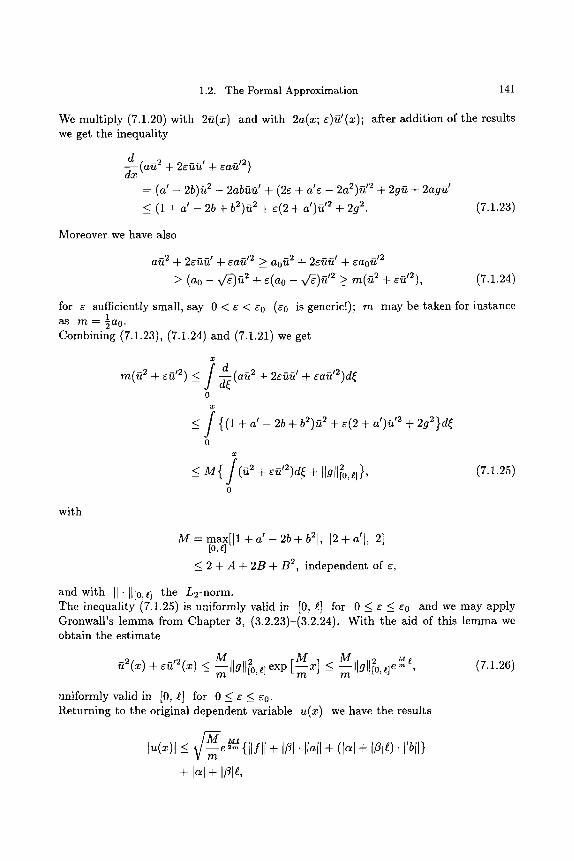
1.2. The Formal Approximation 141
We multiply (7.1.20) with 2fi(x) and with 2a(x; e)fi' (x); after addition of the results we get the inequality
d ( a ~ 2 + 2e~, ' + ea~ '2) d x
= (a I - 2b)~ 2 - 2 a b ~ t ' + (2s + a 's - 2a2)u '2 + 2gfi + 2agf t '
< (1 + a' - 25 + b2)fi 2 + e(2 + a')fi '2 + 2g 2. (7.1.23)
Moreover we have also
a~ 2 + 2e~fi' + ~a~ '2 >_ ao ~2 -+- 2efifi' + ~ao ~'2
>_ (ao - V/e)~ 2 + e(ao - v/e)fi '2 > m(fi 2 + eft'2), (7.1.24)
for e sufficiently small, say 0 < e < eo (so is generic!); m may be taken for instance 1 as m - - ~ao.
Combining (7.1.23), (7.1.24) and (7.1.21) we get
x
m ( ~ 2 + e~ '2) _< f ~ ( a f i 2 + 2 ~ ' + ea f t ' 2 )d~
0
< ] { (1 + a' - 2b + b2)~ 2 + e(2 + a')fi '2 + 2g2}d~
0
x
_< M { / ( f i 2 + efi,2)d~ + {Igtt~o,l]}, (7.1.25)
0
with
M = max[]l + a ' - 2b + b2l, 12 + a'l, 2] [0,~]
< 2 + A + 2B + B 2 independent of v,
and with I]" [1[o,~] the L2-norm. The inequality (7.1.25) is uniformly valid in [0, g] for 0 __< E _< eo and we may apply Gronwall's lemma from Chapter 3, (3.2.23)-(3.2.24). With the aid of this lemma we obtain the estimate
~2(x ) + efi,2(x ) < M ilgll 2 M M M e m [o,l] exp [~-x] < --]]g]l~o, (7.1.26) _ - - _ t]e m , ? n
uniformly valid in [0, t] for 0 _< c < so. Returning to the original dependent variable u ( x ) we have the results
v / M ~____~t f u ( x ) l <_ - ~ e {{[fl[ + If~l �9 [lall + (ial + I~lg). llbll}
+ I~] + ]Zle,
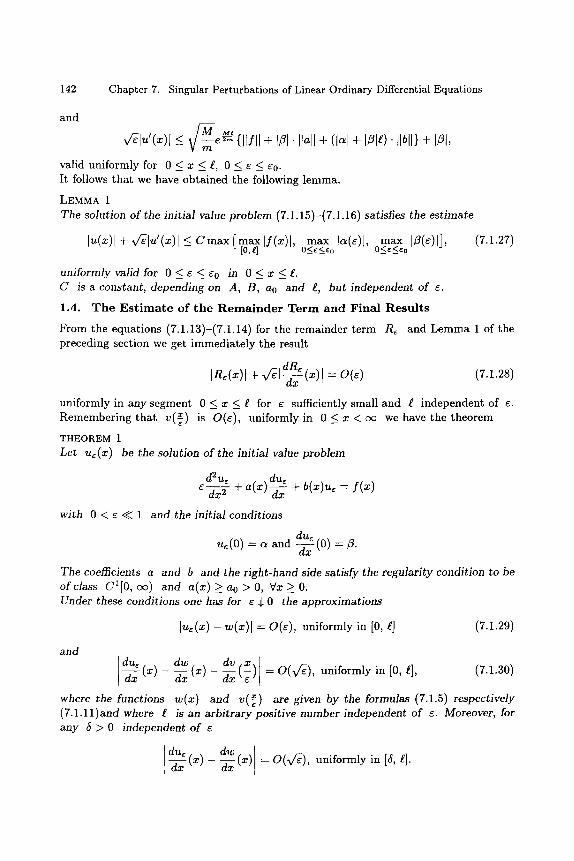
142 Chapter 7. Singular Perturbations of Linear Ordinary Differential Equations
and / - M M,
x/elu'(x)l ~- V -~e2. . {llfll -F Ifl[ " Ilall -b (Ic~l q-I/3[g). [Ibl]} + 1/31,
valid uniformly for 0 _ x _ s 0 < e < e0. It follows that we have obtained the following lemma.
LEMMA 1 The solution of the initial value problem (7.1.15)-(7.1.16) satisfies the estimate
lu(~)l + v~l,~'(~)l < C m a x [maxlf(x)[ max In(e)[ max [/3(e)[] (7.1.27) - - [ O , e ] ' O < e < e o ' O < e < e o '
uniformly valid for 0 <_ e <_ eo in 0 <_ x <_ s C is a constant, depending on A, B, ao and s but independent of e.
1.4. T h e E s t i m a t e of t h e R e m a i n d e r T e r m a n d F ina l R e s u l t s
From the equations (7.1.13)-(7.1.14) for the remainder term Rc and Lemma 1 of the preceding section we get immediately the result
dRe ]R~(x)l + v ~ l - ~ x (x)[ : O(e) (7.1.28)
uniformly in any segment 0 < x < t~ for e sufficiently small and ~ independent of e. Remembering that v(~) is O(e), uniformly in 0 <_ x < oc we have the theorem
THEOREM 1 Let u~(x) be the solution of the initial value problem
d2ue du~ e ~ + a(x)--~x + b(x)u, - f ( x )
with 0 < e << 1 and the initial conditions
due ue(0) = a and --~--x (0) : / 3 .
The coefficients a and b and the right-hand side satisfy the regularity condition to be of class Cl[0, oc) and a(x) >_ ao > O, Vx >_ O. Under these conditions one has for e $ 0 the approximations
[u~(x)- w ( x ) [ - O(e), uniformly in [0, ~] (7.1.29)
and due dw dv x --~-x ( x ) - -d--~x ( x ) - ~xx(~) - O(vfe), uniformly in [0, s (7.1.30)
where the functions w(x) and v(~) are given by the formulas (7.1.5) respectively (7.1.11)and where ~ is an arbitrary positive number independent of e. Moreover, for any 6 > 0 independent of e
due dw --~-x (x) - -d-~x (x) - o(x/~), uniformly in [6, s
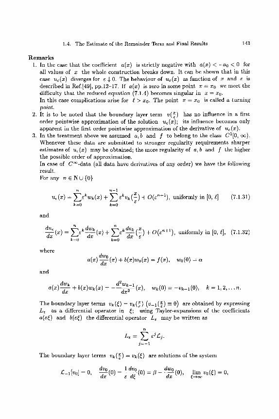
1.4. The Estimate of the Remainder Term and Final Results 143
R e m a r k s 1. In the case tha t the coefficient a(x) is strictly negative with a(x) < - a 0 < 0 for
all values of x the whole construction breaks down. It can be shown tha t in this case ue(x) diverges for ~ $ 0. The behaviour of ue(x) as function of x and c is described in Ref.[49], pp.12-17. If a(x) is zero in some point x - x0 we meet the difficulty tha t the reduced equation (7.1.4) becomes singular in x - x0. In this case complications arise for i > x0. The point x = x0 is called a turning point.
2. It is to be noted tha t the boundary layer te rm v(~) has no influence in a first order pointwise approximat ion of the solution ue(x); its influence becomes only apparent in the first order pointwise approximat ion of the derivative of ue(x).
3. In the t rea tment above we assumed a, b and f to belong to the class C1[0, cx~). Whenever these da ta are submit ted to stronger regulari ty requirements sharper est imates of ue(x) may be obtained; the more regulari ty of a, b and f the higher the possible order of approximation. In case of C~ (all da ta have derivatives of any order) we have the following result. For any n C N U { O }
and
n n--i X
k=O k=O
(7.1.31)
due n dwk n dvk x dx (x) - E e k ~ ( x ) + Eek--d-X-X (--~) + O(e'~+l), uniformly in [0, ~], (7.1.32)
k=0 k=0
where
and
dwo a(x)--d-~x (X ) + b(x)wo(x) = f (x), 0(0) =
a(x) dwk + - d2Wk_l dx 2 (x), wk(O) -- --Vk-l (O), k -- 1, 2 , . . . n .
The boundary layer terms vk(~) = vk(~) ( V - I ( ~ ) ~ O) are obtained by expressing Le as a differential operator in ~; using Taylor-expansions of the coefficients a(r c) and b(r the differential opera tor Le may be wri t ten as
n
j = - - i
The boundary layer terms vk(~) = vk(~) are solutions of the system
dvo I dvo dwo /~_I[VO] = O, --d-~x (0) = ~---~-(0) = f l - ---dT(O), r vo(~) = O,
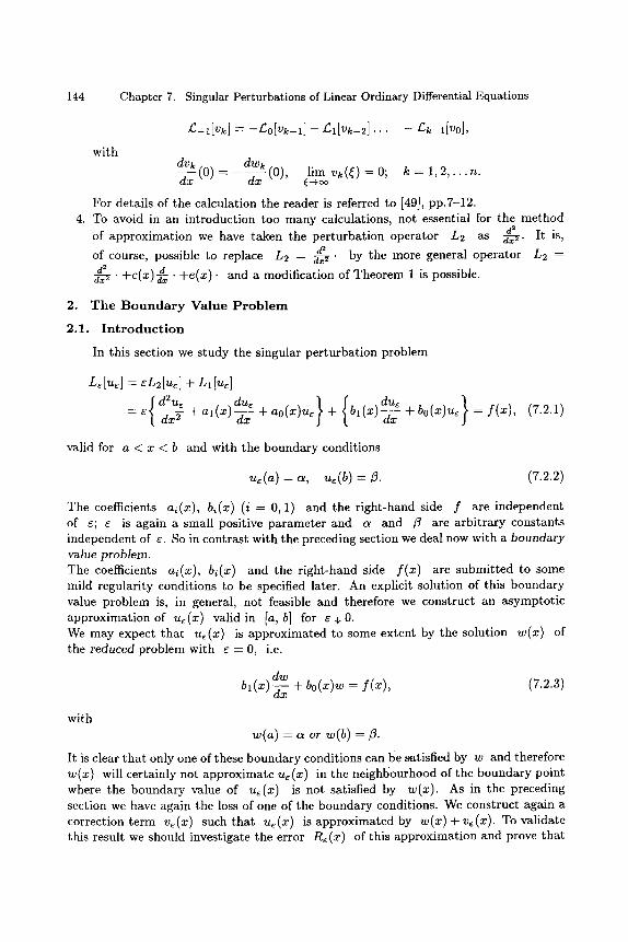
144 Chapter 7. Singular Perturbations of Linear Ordinary Differential Equations
g-~[,~] = -g0[ ,~-~]- L ~ [ ~ _ : ] . . . - ~ - ~ [ ~ 0 ] ,
with dv~ dwk dx ( 0 ) - - - - - ~ - x (0) lim vk(~)= 0; k = 1 2 , . . . n .
' ~---~ OO
For details of the calculation the reader is referred to [49], pp.7-12. 4. To avoid in an introduct ion too many calculations, not essential for the method
d 2 of approximat ion we have taken the per turba t ion operator L2 as d--~" It is,
d 2 of course, possible to replace L2 - dx2" by the more general operator L2 -
42 �9 +c(x) d . +e(x)" and a modification of Theorem 1 is possible. dx 2 -~x
2. T h e B o u n d a r y Value P r o b l e m
2.1. I n t r o d u c t i o n
In this section we s tudy the singular per turba t ion problem
L~[u~] = eL2[u~] + Ll[u~]
= e ~ + al(X)-d-x- x + ao(x)ue + bl(X)--~x + bo(x)ue = f(x), (7.2.1)
valid for a < x < b and with the boundary conditions
u~(a) = ~, ~ ( b ) = ~. (7.2.2)
The coefficients ai(x), bi(x) (i - 0, 1) and the r ight-hand side f are independent of ~; ~ is again a small positive paramete r and c~ and ~ are arb i t rary constants independent of ~. So in contrast with the preceding section we deal now with a boundary va]ue prob]em. The coefficients ai(x), bi(x) and the r ight-hand side f(x) are submi t ted to some mild regulari ty conditions to be specified later. An explicit solution of this boundary value problem is, in general, not feasible and therefore we construct an asymptot ic approximat ion of u~(x) valid in [a, b] for c $ 0. We may expect tha t u~(x) is approximated to some extent by the solution w(x) of the reduced problem with c - 0, i.e.
d w bl (x)--~x + bo(x)w = f (x), (7.2.3)
with ~(~) = ~ o~ ~ ( b ) = ~.
It is clear tha t only one of these boundary conditions can Be satisfied by w and therefore w(x) will certainly not approximate ue(x) in the neighb~ourhood of the boundary point where the boundary value of us(x) is not satisfied by w(x). As in the preceding section we have again the loss of one of the boundary conditions. We construct again a correction te rm v~(x)such tha t u~(x)is approximated by w(x)+ v~(x). To validate this result we should investigate the error R~(x) of this approximat ion and prove tha t
2.2. The Maximum Principle for Ordinary Differential Operators 145
Re(x) approaches zero for e $ 0. This will be performed by formulat ing a boundary value problem for Re(x) and by giving consecutively an a priori es t imate for R~(x). This es t imate is obtained with the aid of the maximum principle for ordinary differential equations of the second order, see l i t . I l l9] , Ch.1. Because this principle can also be used for the right choice of the boundary value of w(x) we t reat first this m a x i m u m principle and its consequences.
2.2. The Maximum Principle for O r d i n a r y D i f f e r e n t i a l Operators
The Max imum Principle may be formulated as follows: Let L be the differential operator
d 2 d . +c(x) �9 "= M + c(x) (7.2.4) L = a(x)-~x2.+b(x)-~x
with a(x) > 0 and a,b and c continuous in a bounded segment [71, 72] C JR. If a twice differentiable function O(x) a t ta ins a local m a x i m u m in an interior point P of (71,72) then M[(I,] < 0 in P. If on the contrary ~ satisfies in (71,72) the differential inequali ty M[O] > 0 then it is clear tha t �9 cannot a t ta in a local m a x i m u m in (71,72); if moreover ~ is also continuous in [71, 72] then the m a x i m u m of ~ can only be a t ta ined in one or in bo th endpoints x = 71, x - 72. This is the m a x i m u m principle in its most simple form. If the m a x i m u m of ~ in an interior point P is positive and if c(P) < 0 then also L [ O ] < 0 in P. As a corollary of this principle we have the following useful lemma.
LEMMA 2
If the twice continuously differentiable functions r and gJ(x) satisfy in the bounded interval (Tt, 72) C IR the relation
IL[~][ < L [ - r Vx e (71,72), (7.2.5)
where L is the differential operator given by (7.2.4) with c(x) ~_ 0 in (71,72) and if
I~(~y~)l ~ ~(~,), i - 1,2 (7.2.6)
then also Ir _< r w: �9 [71, 72]. (7.2.7)
P r o o f
Suppose ~ - ~ possesses a positive m a x i m u m in an interior point P of (3'1,3'2) then we have according to the m a x i m u m principle
L [ r ~ ] f . < o,
which contradicts the relat ion (7.2.5) and so ~ - ~ does not have a positive m a x i m u m in (71,3'2)- Since we have also ~ - ~ < 0 in x = 71 and x = 72 we must have r �9 _< 0 in [3'1, 72]. Similarly one proves - 4 - �9 _< 0 in [71, 72] and hence the relat ion (7.2.7) holds. K]
146 Chapter 7. Singular Perturbations of Linear Ordinary Differential Equations
The function ~(x) yields an upper bound for the absolute value of r in [')'1, ")'2], rea- son why ~(x) is called a barrier function for the function r A priori est imates of solutions of boundary value problems for second order ordinary differential equa- tions may be obtained by the construction of suitable barrier functions tha t satisfy the conditions of Lemma 2.
R e m a r k The lemma can be generalized by replacing the strict inequality (7.2.5) by
[L[+][ < L [ - ~ ] , Vx �9 (71,')'2).
By this small generalization one obtains immediately as an interesting corollary the uniqueness of solutions of boundary value problems. The proof is simple: suppose Ul(X) and u2(x) are two solutions of the boundary value problem with L[u] : f ( x ) , then the function ~(x) - 0 is a barrier function for the difference u 2 ( x ) - Ul(X). For a proof of this generalization of Lemma 2 we refer the reader to l i t .I l l9], Ch.1.
2.3. A n A Priori E s t i m a t e of the So lu t ion of the B o u n d a r y Value P r o b l e m
We return now to our boundary value problem (7.2.1)-(7.2.2). We assume for the moment tha t the coefficients ai(x), bi(x) (i - 0, 1) and the r ight-hand side / ( x ) are continuous in [a, b]. Moreover, we suppose b l ( X ) r 0 in [a, b] and b o ( x ) < 0 in [a, b]. The first assumption bl (x) r 0 is in so far essential tha t the reduced equation (7.2.3) does not become singular. In case bl(x0) - 0 for some point x0 E [a, b] the solution w(x) of (7.2.3) has a singularity in x = x0 and the theory becomes much more complicated. The point x = x0 is called a turning point; see section 3 of this chapter. The condition bo(x) < 0 is necessary in order to guarantee the uniqueness of the solution of our boundary value problem (7.2.1)-(7.2.2). Wi th bo(x) < 0 we have also bo(x) + eao(x) < 0 for e sufficiently small, uniformly for all x E [a, b] and this guarantees according to Lemma 2 the uniqueness of the solution of the boundary value problem; (see also Remark 3 at the end of this chapter). We take bl(X) > 0; this is not a restriction because the other case bl(X) < 0 can be t reated in a similar way. The maximum principle provides a simple and useful a priori es t imate for the solution u~(x) of (7.2.1)-(7.2.2). For this purpose we consider the function u*(x) : ue(x) - fl, tha t satisfies the boundary value problem
L~[u:] : f ( x ) - t3bo(x)- et3ao(x)= f*(x; e), a < x ( b,
with the boundary conditions
ue (a) = c~ - fl, u e (b) = 0.
The linear function (I)(x) = M ( b - x) with M some positive constant satisfies the inequality
L~[M(x - b)] = E { a l ( x ) M -4- ao (x )M(x - b) } -f- b l ( x ) M -4- bo(x)M(x - b)
> M { b l ( x ) A- ~al(x) -+- eao(x)(x - b)}, a < x < b.
2.2. The Maximum Principle for Ordinary Differential Operators 147
Hence with 7 - min bl (x) we have the inequality [a,b]
1 M L ~ [ M ( x - b)] > ~ ~,,
valid for a < x < b and for c sufficiently small, say 0 < c < e0. Choosing
M = max [~, b],o_<~_<~o ' b - a
we get
(7.2.8)
IL~[u*~]l < L ~ [ - M ( b - x)],
M ( b - a) > I ~ - al = lu~(a)l,
M(b - b) = 0 - ]u~ (b) l.
a < x < b ,
It follows tha t the function w(x) = M ( b - x) is a barrier function for the function u;(x) and so we get for the solution u~ of the boundary value problem (7.2.1)-(7.2.2) the a priori es t imate
lu~(x) - j3 I < M ( b - x), V x E [ a , b ] a n d 0 < e _ < r (7.2.9)
with M given by (7.2.8) and M is independent of e. A similar a priori es t imate gt(x) = M ( x - a ) for the function u e ( x ) - ~ is not possible, because
L s [ - M ( x - a)] - e ( - M a l ( x ) - Mao(x ) (x - a)} - Mbl(x ) - Mbo(x) (x - a)
and the e-independent par t of the r ight-hand side becomes negative in a right neigh- bourhood of x = a and so M ( x - a) is not a candidate for a barrier function of u ~ ( x ) - ~. The graph of the unknown function u~(x) lies in the region
t3 + M ( x - b) < u~(x) < j3 + M ( b - x). (7.2.10)
It follows tha t lim d_~ is bounded for all values of r with 0 < c < e0. As long as y---+O dx
and d 2 ue dx ~ are uniformly bounded in some par t of (a, b) the differential equat ion
(7.2.1) is well approximated by its reduced part bl dw -g~ + bow = f (x ) , but this needs not
to be true whenever ~ and ~ are not bounded for e sufficiently small. If for dx dx 2
due 1 d2 u~ - d2 u~ in the instance ~ - O(~) and d--~ -- O ( ~ ) it is possible tha t the te rm ~d--~
per turbing par t and the te rm bl d_~ in the reduced par t of of the equat ion may balance dx
each other. Due to the result (7.2.10) this cannot happen in the left neighbourhood of the point x = b and therefore we guess tha t the solution u~ of the boundary value problem (7.2.1)-(7.2.2) is approximated in this neighbourhood by the solution of the boundary value problem
d w bl(x)-~x + bo(x)w - f ( x ) with w(b) - / 3 .
148 Chapter 7. Singular Perturbations of Linear Ordinary Differential Equations
In case bl (x) were negative in [a, b] we would make the guess tha t the solution ue is approximated in a right neighbourhood of the point x = a by the solution of the boundary value problem
dw b 1 (x)-~x + bo(x)w = f ( x ) w i t h w ( a ) - - o~.
It will appear in the next section tha t this heuristic reasoning leads indeed to the con- s t ruct ion of a formal approximat ion of u~, tha t is to a function which satisfies the differential equat ion and the boundary conditions up to some positive order of ~.
2.4. T h e F o r m a l A p p r o x i m a t i o n
For the construct ion of the formal approximat ion we need some mild regulari ty conditions for the coefficients and the r ight-hand side of the differential equation. These conditions are:
bo(x) �9 Cl[a, b], bl(x) �9 C2[a, b], ao(x) �9 C[a, b], al(x) �9 Cl[a, b] and
f ( x ) �9 e l [ a , b]. (7.2.11)
Cm[a, b] is the class of all functions m times continuously differentiable in [a, b]; C[a, b] is the class of all functions continuous in [a, b]. Moreover, we suppose
bl(x) > O, bo(x) < 0, Vx �9 [a, b]. (7.2.12)
Using the heuristic reasoning of the last subsection we consider first the reduced problem
dw bl (x)--~x + bo(x)w - f (x ) ,
with the boundary condit ion
The solution reads
where
a < x < b, (7.2.13)
w(b) - ft. (7.2.14)
b
w(x)--eq('){'- f e-q(~) bl(~)f(~)d~) , (7.2.15)
x
b
f bo(,~) d,~ q(x) = ~ . x
This function is, in general, not a good approximat ion of u~ in the neighbourhood of the point x = a because w(a) =/= a. So we need a correcction te rm tha t accounts for the boundary condit ion ue(a) - a . To investigate what happens in the neighbourhood of x - a we use a "microscope" defined by the t ransformat ion
x = a 9- ~ , (7.2.16)
2.4. The Formal Approximation 149
where u is a positive number that will be used for the "focussing" of the "microscope". The differential operator Le expressed in the new coordinate ~ reads
1--2u d2 L e = ~ d~ 2
d _ _ . + 61-Val(a + ~v~)__~ . +eao(a + ev~) .
d + e-Vbl(a + ~'~)-7;," +bo(a + c~'~) �9 �9
a~
If v is larger than 1 ~, the most dominant terms are e 1-2v d2 d~2" and e-Vbl(a+e~@)~ .. To get a balance in the differential equation between the perturbing part and the reduced part we put u = 1. Because of the supposed regularity (7.2.11) of the coefficients we have in [a, b] the expansions
a l ( a + ~ ) - - a j ( a ) + e ~ a ~ ( a + ~ l ( x - a ) ) , 0<z91 < 1,
bl(a + ~ ) = bl(a) + efb~(a)+ 1~2~22 ~ bl''(a + ~ 2 ( X - a))
b o ( a + c f ) = b o ( a ) + e @ b ' o ( a + z 9 3 ( x - a ) ) , 0 < ~ 3 < 1,
0 < ~ 2 < 1 ,
where primes denote differentiations with respect to x. Inserting these expansions into the differential operator LE we get
Le = e - ' I s n t- s -{- es (7.2.17)
where d 2 d
s = ~-~5" +bl (a)d~ c .,
/:o = {al(a) + @b~(a)}~. +bo(a) e ,
s -- {~a~(a -+- ~01~ ) -~- ~2b~/(a + e02~)} d--~"
+ ao(a + e~). +C~b'o(a + 6~3~) �9
To satisfy the differential equation up to O(e) and to fulfil the boundary condition at x -- a we make the following a t tempt for the formal approximation of ue
ue(x) = w(x) + vo( x - a) + evl ( x - a ) + RE(x)
= ~(=) + v0(~) + ~(~) + R~(~), (7.2.18)
with
s and s = -s
and the boundary conditions
0 < ~ < co, (7.2.19)
v0(O) = a- w(a), v0(oo) = 0 and Vl(O) = vl (oo) = O. (7.2.20)
150 Chapter 7. Singular Perturbations of Linear Ordinary Differential Equations
The conditions at ~ = c~ provide the desired result that the correction terms v0 and Vl have only a significant value in an e-neighbourhood of the point x = a. From (7.2.19) and (7.2.20) we get
d2vo dvo + bl(a)--7;- ~ -- 0, vo(a) -- c~ - w(a), v0(cx)) = 0,
d~--- ~ a ~
and hence
v o ( X - a ) __ v0(~) ---- { a - w ( a ) } e x p [ - b l ( a ) ~ ] E
= {a - w (a ) } exp [ - bl (a) x - a]. (7.2.21)
The function vl (~) satisfies the differential equation
d2vl
d~ 2 dvl = (A + B,~) exp[-bl (a)~] + bl(a)-~-
where A and B are some constants. With the aid of Vl(0) = vl (oc) = 0 we obtain
v l ( X - - a) = = Vl (~) (Cl~ q- 62~ 2) exp [ bl(a)~]
x - a x - a 2 x - a ] = { C 1 ~ + C 2 ( ) } e x p [ - b l ( a ) e ' J
c (7.2.22)
where C1 and 02 are again some constants. Substi tution of (7.2.18) into the differential equation (7.2.1) yields for the term Re the differential equation
Le[Re] = Le[ue] - L~[w] - { e - I L _ I + s + es + evl]
= f ( x ) - { f ( x ) --k eL2[w]} - e/:0[vx] - eZ:l[v0 + evl]
{ } d2w dw e'{al(a) + ~bi (a)} d~ = - ~ ~ + al(x)--d--~x + ao (x )w -
-- r - r + CVl].
Due to the regularity of w (w e C2[a, b]), the exponential character of v0(() and Vl(() with bl(a) > 0, the behaviour of the coefficients in the operator s and the regularity of the coefficients ai and bi as stated in (7.2.11), we obtain
L e [ R ~ ] - O(6), uniformly in [a, b], (7.2.23)
for e sufficiently small, say 0 < e < co. As to the boundary conditions we have
Re(a) - 0 and Re(b) -- ue(b) - w(b) - vo( b -_.____aa) _ CVl (b - a ) ~ O. (7.2.24)
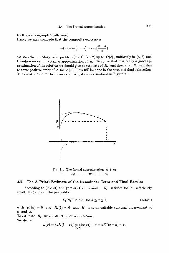
2.4. The Formal Approximation 151
(~ 0 means asymptot ica l ly zero). Hence we may conclude tha t the composite expression
w(x ) + vo (x - a) + evl ( x - a) C
satisfies the boundary value problem (7.2.1)-(7.2.2) up to O ( e ) , uniformly in [a, b] and therefore we call it a formal approximat ion of ue. To prove tha t it is really a good ap- proximat ion of the solution we should give an es t imate of Re and show tha t Re vanishes as some positive order of e for e $ 0. This will be done in the next and final subsection. The construct ion of the formal approximat ion is visualized in Figure 7.1.
~
~
!
!
!
!
!
-~ X
Fig. 7.1 The formal approximation w + v0 ue; w; . . . . . . vo
2.5. T h e A P r i o r i E s t i m a t e o f t h e R e m a i n d e r T e r m a n d F i n a l R e s u l t s
According to (7.2.23) and (7.2.24) the remainder Re satisfies for e sufficiently small, 0 < e < e0, the inequali ty
ILe[Re]I < g e , for a < x _~ b, (7.2.25)
with Re(a) = 0 and Re(b) ~ 0 and K is some suitable cons tant independent of x and e. To es t imate Re we construct a barrier function. We define
w(x) - { ~ g ( b - x ) / m i n b l ( x ) } + e - e g * ( b - x) + e, [a,b]
152 Chapter 7. Singular Perturbations of Linear Ordinary Differential Equations
and we get due to bo(x) < 0 and bl(x) > 0
d2w dw } do; Le[-w] = - ~ ~ + a l ( x ) ~ x + ao(x)w - bl(x)-~x - bo(x)w
= ~2g*a l ( x ) - ~ 2 K * ( b - x)ao(x) - 62a0(x)
+ { r - e b o ( x ) { g * ( b - x) + 1} :> g o , [~,b]
for e sufficiently small, say 0 < e < e0, where ~0 is again a generic constant , tha t is to say a value such tha t earlier s ta tements involving ~0 remain valid. Therefore
[ L e [ R e ] l < L e [ - w ] , f o r a _ x _ b , 0 < e < E 0 ,
and at the boundaries we have
w(a) > 0 ~ R E ( a ) - - 0 , and w(b) - e > R E ( b ) ~ O.
It follows tha t w(x) is a barrier function for Re and with the aid of L e m m a 2 we obtain
[Re(x)[ ~ w ( x ) < eK*(b - a) q- e : - eM, a ~ x ~ b, O < e < eo, (7.2.26)
where M is a number independent of r As an immedia te result we now get
Ue(X ) : W(X) + VO( ~- -- a) -[- ~1)1 ( x -- a) -[- O(E), uniformly in a _< x _< b.
However, because the function vl (~--~) = Vl (~) is bounded for 0 < ( < c~ we may simplify this result to
ue(x) -- w(x) + Vo( x - a ) + o(E), uniformly in a < x < b. G
(7.2.27)
Summariz ing we have the following theorem
THEOREM 2 Let ue(x) be the solution of the boundary value problem
{ d2ue due } due a < x < b
with 0 < ~ << 1 and uE(a) -- a and ue(b) - ~. The coet~cients and the right-hand side satisfy the regularity conditions (7.2.11) with bl(x) > 0 and bo(x) < 0 on [a, b]. Under these conditions the following approximations are uniform!y valid for e suffi- ciently sma]l
ue(x) = w(x) + vo( x -- a) + 0(~) , a ~_ x ~_ b G
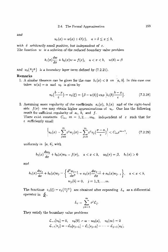
2.4. The Formal Approximation 153
and u~(x) = w(x) + O(e), a + 5 <_ x < b,
with 5 arbitrarily small positive, but independent of r The function w is a solution of the reduced boundary value problem
dw bi(x)-d-~- x + b 0 ( x ) w = f ( x ) , a < x < b , w(b)=
and vo(X= ---~) is a boundary layer term defined by (7.2.21).
R e m a r k s 1. A similar theorem can be given for the case bl (x) < 0 on [a, b]. In this case one
takes w(a)= a and v0 is given by
b ~ X v0 ( - - - ~ ) = v0(~) = { /3- w(b)} exp [b t (b )b - x]. (7.2.28)
2. Assuming more regularity of the coefficients ai(x), bi(x) and of the right-hand side f (x) one may obtain higher approximations of u~. One has the following result for sufficient regularity of ai, bi and f . There exist constants Cm, m = 1 ,2 , . . .m0 , independent of e such that for
sufficiently small
m m
ue(x) - E eJwj(x) - E eJvJ( x-- a) j =0 j =0
< Cmcm+ 1, (7.2.29)
uniformly in [a, b], with
dwo b l ( x ) - ~ z + bo(x)wo = f (x), a < x < b, wo(x) = 13, bi(x) > 0
and
dwj { d2wj-1 dWj_ l ! bl(x)---~x + bo(x)wj = dx 2 + al(x) dx + ao(x)wj_l ,
wj(b) = 0 , j = l , 2 , . . . m .
a < x < b ,
The functions vj(~)= v j ( ~ ) are obtained after expanding L~ as a differential operator in ~ ,
m
L~ = E ejLj" j - - - 1
They satisfy the boundary value problems
L- i [v0 ] = 0, v0(0) -- a - - wo(a), Vo(OO) = 0
~ _ l [ V j ] - - - - ~ 0 [ V j _ l ] - ~l[Vj_2] . . . . . ~j_l [V0] ,
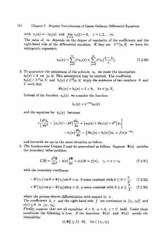
154 Chapter 7. Singular Perturbations of Linear Ordinary Differential Equations
with v j ( a ) = - w j ( a ) and lim v j ( ~ ) = 0 , j = l , 2 , . . . m .
The value of m depends on the degree of regularity of the coefficients and the right-hand side of the differential equation. If they are C~176 b] we have the asymptotic expansion
oo oo ~ (~) ~ ~ ~J~j (~) + ~ ~J,j ).
C j =0 j =0 (7.2.30)
3. To guarantee the uniqueness of the solution u~ we made the assumption bo(x) < 0 on [a, b]. This assumption may be omitted. The conditions bo(x) E Cl[a, b] and bl (x) E C2[a, b] imply the existence of two numbers t0 and 5 such that
tobl(x) + bo(x) < 5 < O, VxE[a ,b] .
Instead of the function we(x) we consider the function
~(~) = ~ - ~ ( ~ )
and the equation for fie(x) becomes
d2 ztr d fie + { a l ( x ) + 20}-d-~x + {a0(x)+ toal(x)+ to2}fi~
dfi~ -[- b l ( x ) - - - ~ x --[-- { t o b l ( X ) -[- b o ( x ) } u e - - f(x)e -tgx,
and herewith we are in the same situation as before. 4. The fundamental Lemma 2 may be generalized as follows. Suppose r satisfies
the boundary value problem
L [ r = d 2 r d R + b ( ~ ) ~ + ~(~)~ = f(~), 3'1 < x < "Y2 (7.2.31)
with the boundary conditions
7r - r 0 + 4(71)sin 0 = a, 0 some constant with 0 < 0 < ~,
+ r cosy + r sin~o = fl, ~0 some constant with 0 _< ~o _< 2 '
(7.2.32)
(7.2.33)
where the primes denote differentiation with respect to x . The coetlicients b, c and the right-hand side f are continuous in ['YI, 72)] and c(~) <_ o i . [~, ~2]. Finally, suppose that not all equalities 0 = O, ~ = O, c - 0 hold. Under these conditions the following is true. I f the functions r and ql(x) satisfy the inequalities
IL[r < L[ -~] , Vx E (~1, ~2)
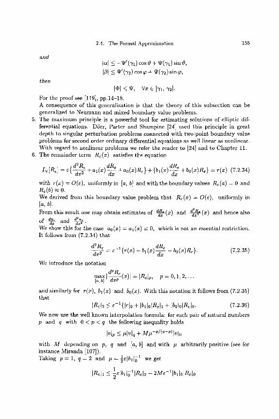
2.4. The Formal Approximation 155
and [~[ <_ - ~ ' ( ~ ) ~ose + ~(v~) sinO,
I/31 < 9 ' (')2) cos ~o + ~ (~/2) sin ~o,
then
For the proof see [119], pp.14-18. A consequence of this generalization is that the theory of this subsection can be generalized to Neumann and mixed boundary value problems.
5. The maximum principle is a powerful tool for estimating solutions of elliptic dif- ferential equations. Dhrr, Parter and Shampine [24] used this principle in great depth to singular perturbat ion problems connected with two-point boundary value problems for second order ordinary differential equations as well linear as nonlinear. With regard to nonlinear problems we refer the reader to [24] and to Chapter 11.
6. The remainder term Re(x) satisfies the equation
d2Re dRe dRe Le[Rs] = e{ dx 2 +al(x)-~x +aO(x)Re}+{bl(x)-~x +bo(x)Re} = r(x) (7.2.34)
with r (x )= O(e), uniformly in [a, b] and with the boundary values Re(a)= 0 and Re(b) ..~ O. We derived from this boundary value problem that Re(x) = O(e), uniformly in In, hi. From this result one may obtain estimates of d-~R (x) and ~ (x) and hence also dx dx 2
due d2 u~ of ~ and dx2" We show this for the case no(x) = el (x) - O, which is not an essential restriction. It follows from (7.2.34) that
d2Rs dR~ dx 2 = e - l { r ( x ) - bl(x)--~x - bo(x)Re}. (7.2.35)
We introduce the notation
max I dpRe Io, bl ~ ( ~ ) l = IR~lp, p = 0, 1, 2 , . . .
and similarly for r(x), bl (x) and bo(x). With this notation it follows from (7.2.35) that
IR~I2 < c-1{I,'1o + IbllolR~ll + IbololR~lo. (7.2.36) We now use the well known interpolation formula: for each pair of natural numbers p and q with 0 < p < q the following inequality holds
Ivlp < ~1",-,I,~ + M~-~/cq-~)l~lo with M depending on p, q and [a, b] and with # arbitrarily positive (see for instance Miranda [107]). Taking p = l , q = 2 and # = ~eIbl[o 1 we get
1 IR~]I _< -~eIbllolIRel2 + 2Me-llbllolRslo
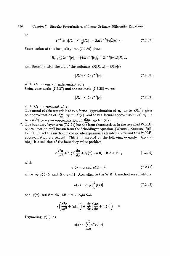
156 Chapter 7. Singular Perturbations of Linear Ordinary Differential Equations
or
1 IR~I2 § 2ME-2[b~I~[R~Io.
Substitution of this inequality into (7.2.36) gives
IR~I2 ~ 26-11~1o + (4ME-21bll 2 + 2~-~lbolo)lR~lo,
(7.2.37)
and therefore with the aid of the estimate O(IR~10)- O(Irl0)
IR~12 _~ C2~-2lr[0 (7.2.38)
with C2 a constant independent of e. Using once again (7.2.37) and the estimate (7.2.38) we get
IRell _~ C16-11rlo (7.2.39)
with C1 independent of e. The moral of this remark is that a formal approximation of u~ up to 0(62) gives an approximation of ~ up to O(e) and that a formal approxmation of ue up
to 0(63) gives an approximation of ~ up to 0(6) dx2 7. The boundary layer term (7.2.21) has the form characteristic in the so-called W.K.B.
approximation, well known from the SchrSdinger equation, (Wentzel, Kramers, Bril- louin). In fact the method of composite expansion as treated above and this W.K.B. approximation are related. This is illustrated by the following example. Suppose u(x) is a solution of the boundary value problem
d2u du ~ + b ~ ( ~ ) ~ + bo(~)u = o, 0 < x < 1, (7.2.40)
with u(0) = a and u(1) = fl (7.2.41)
while bl (x) > 0 and 0 < 6 << 1. According to the W.K.B. method we substitute
~(~) = ~xp [lq(~)] (7.2.42)
and q(x) satisfies the differential equation
Expanding q(x) as
) dq(dq ) ~ + b o ( ~ ) + ~ ~+b~(~) =o.
oo q(~) ~ ~ ~"q~(~)
n--0
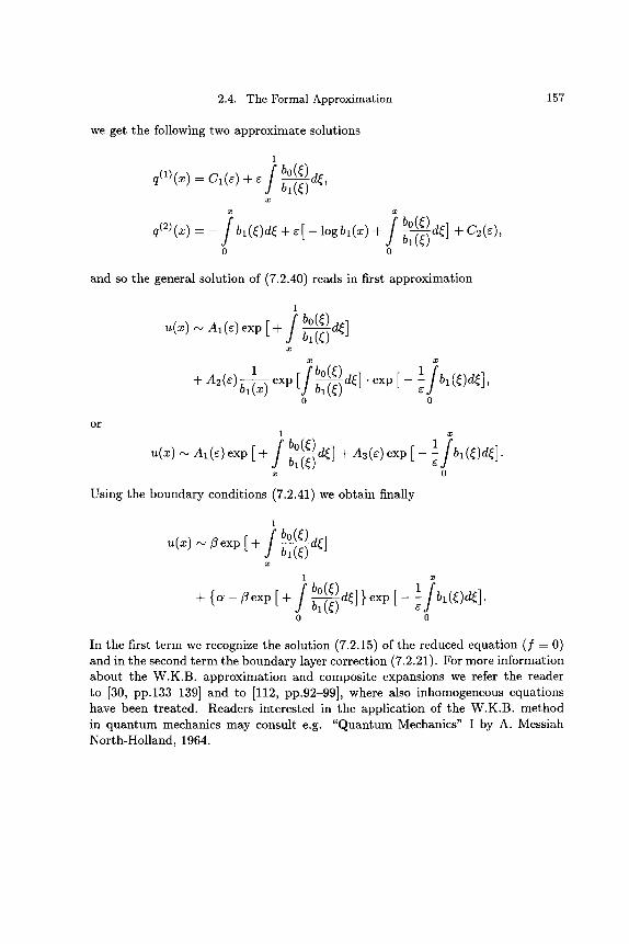
2.4. The Formal Approximation 157
we get the following two approximate solutions
1
/ b0(() d(, q(1) (~) = c~ (~) + ~ bl(~)
x
bo(() q(~)(~) - - bl(r162 + ~ [ - logbl(~) + b - ~ a r + C~(~),
o o
and so the general solution of (7.2.40) reads in first approximation
1
I ~,q) x
x x 1 [ / ~ 1/ + A2(e) bl(x) exp d(] .exp [ - - bl(()d(],
1 ~,q) E 0 0
or 1 x
f b0(() d(] + A3(r [ - e u(x) ~ A1 (e) exp [ + bl (~) x 0
Using the boundary conditions (7.2.41) we obtain finally
1
f b0(~) ~(~) ~ ~exp[+ b-~~] x
1 x
+ {a - - ~exp [-b b - ~ d ~ ] } exp [ - c j 0 0
In the first term we recognize the solution (7.2.15) of the reduced equation (f - 0) and in the second term the boundary layer correction (7.2.21). For more information about the W.K.B. approximation and composite expansions we refer the reader to [30, pp.133-139] and to [112, pp.92-99], where also inhomogeneous equations have been treated. Readers interested in the application of the W.K.B. method in quantum mechanics may consult e.g. "Quantum Mechanics" I by A. Messiah North-Holland, 1964.

158 Chapter 7. Singular Perturbations of Linear Ordinary Differential Equations
3. B o u n d a r y V a l u e P r o b l e m s with Turning Points
3.1. Introduct ion
In the preceding section we made the essential assumption tha t the coefficient bl (x) of dw in the reduced equation (7.2.13) has a fixed sign in the segment [a, b]. In case bl (x) > 0 we have a boundary layer at the left-hand side x : a and in case bl (x) < 0 there is a boundary layer at the r ight-hand side x : b. In this section we drop the assumption bl(x) =/: 0 in [a, b] and we discuss again the asymptot ic approximat ion of the boundary value problem and the appearance of boundary layers and eventually also an interior layer in the neighbourhood of a point where bt (x) changes its sign. In order not to complicate our t r ea tment we consider the following simplification of the boundary value problem (7.2.1)-(7.2.2)
d2ye dye e - ~ x 2 -t- f(x)-ff-ffx -I- g(x)ye -- O, - 1 < x < 1, (7.3.1)
with the boundary conditions
y~(-1) = a, y e ( + l ) = b. (7.3.2)
Further we assume tha t f (x) has only one zero at x = 0 and tha t dr(x) is either dx smaller or larger than zero in [ -1 , +1]. Moreover it will appear useful to assume also tha t f and g, considered as functions of a complex variable, are analytic for a _ x _ b. In the next subsection we address the most interesting case ddl(x) < 0 and in the
following one the other case ~ ( x ) > 0. The case ~ ( x ) < 0 is therefore of part icular interest because the value of the parameter
_~_=_ g(O) (7.3.3) 2
is decisive for the approximat ion of ye(x) in [-1, +1]; in case /3 :/: 2m, m = 0, 1, 2 , . . . the so-called outer approximation in ( - 1 , +1) is identically zero while this approximation is not zero for /9 - 2m. This interesting phenomenon has received the name of "resonance". We finish with some references for further s tudy of differential equations with turning points.
3.2. The Turning Point Prob lem with .f'(x) < 0
To analyze the behaviour of the solution ye(x) of our boundary value problem (7.3.1)-(7.3.2) we use a variation of the multiple scale technique as t rea ted in Chapter 6. We consider Ye as a function of the two independent variables
~r -lv(x), 7/-=-- x, (7.3.4) C
where v(x) will be chosen later in an appropriate way. With the aid of
dye 10ye dv OyE dx e O~ dx Or;
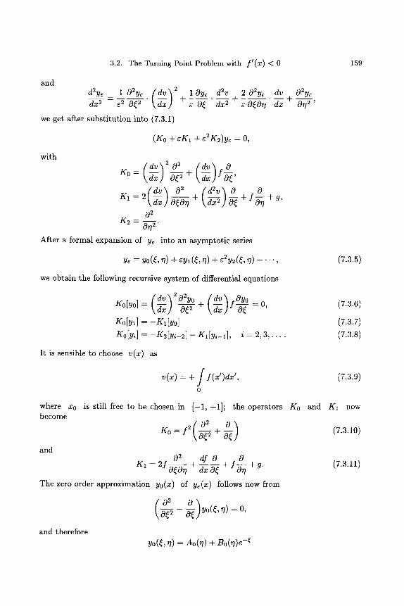
3.2. The Turning Point Problem with I t (x) < 0 159
and d2ye
dx 2 _ 102ye ( d v ~ 2 l O y e d 2 v 202y~ dv
- - ~ 0 ~ 2 " [ , + . . . . . ~ - ~ . e O~ dx 2 eO~Or/ dx
we get after substi tution into (7.3.1)
02ye Or~ 2 '
(Ko + eK1 + e2K2)ye = 0,
with
g o - ~ - ~ + ~ f o--~'
K 1 - 2 -~x O~Or/ + \ dx 2]--~ + Or/+ g'
02 K2 = 0772.
After a formal expansion of ye into an asymptotic series
Yr : Y0(~, 7]) -3 t- Cyl (~, 7]) -Jr E2y2(~, 7]) -~- �9 " " , (7.3.5)
we obtain the following recursive system of differential equations
K0[Y0]= ~ - - ~ + ~xx f - - ~ - = O ,
KO[Yl] ---- -KI[Yo]
Ko[yi] = -K2[yi-2] - Kl[yi-1], i = 2, 3, . . . .
(7.3.6)
(7.3.7) (7.3.8)
It is sensible to choose v(x) as
v(x) - + / f (x')dx', (7.3.9)
~t
where x0 is still free to be chosen in [-1, +1]; the operators Ko and K1 now become
and 0 2 df 0 0
K 1 - 2f + + f -x- + g. (7.3.11) 0~0r/ or/
The zero order approximation yo(x) of ye(x) follows now from
02 0) b7 ~ + b~ yo(~, ~1 - o,
and therefore
yo(C~, r/) = Ao(r/) + Bo(r/)e -~
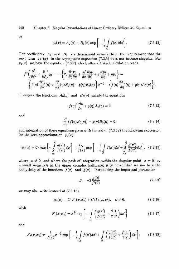
160 Chapter 7. Singular Perturbations of Linear Ordinary Differential Equations
o r yo(x)=Ao(x)+Bo(x)exp[ If Y(~')d~'] ~2
(7.3.12)
The coefficients A0 and B0 are determined as usual from the requirement that the next term eyl (x) in the asymptotic expansion (7.3.5) does not become singular. For Yl (x) we have the equation (7.3.7) which after a trivial calculation reads
f~(~ ~ { ~176 #~176 ~176 } - - ~ "-[- - ~ Y l "-- -- 2 f O ~ O r I + -d--xx ---~-( + f ~ + g Y o =
{ d B o df } { dA0 } f ( r t ) - ~ (r/) + ~xx(r/)B0(r/) - g(rl)Bo(rl) e -~ - f ( r / ) - ~ (r/) + g(rl)Ao(rl) �9
Therefore the functions A0(r/) and B0 (r/) satisfy the equations
dAo f (r/) ---;-- + g(r/)A0(r/) = 0
a t / (7.3.13)
and d
d-~(f(n)Bo(n)) - g(n)Bo(n) = O, (7.3.14) and integration of these equations gives with the aid of (7.3.12) the following expression for the zero approximation yo(x)
x
y0 x/= Clexp [ / g x',dx I C2 f(x') + ~ exp
XO
x
i fi x,) x,+f g/x,/dx, - ; f(~') ~2 Xo
, (7.3.15)
where x # 0 and where the path of integration avoids the singular point x - 0 by a small semicircle in the upper complex halfplane; it is noted that we use here the analyticity of the functions f (x) and g(x). Introducing the important parameter
we may also write instead of (7.3.15)
vo(~) = C~F~(~.xo) + C~F~(~..o). �9 # o, (7.3.16)
with
and
f~ FI(X, xo) = x~" exp
/ (g(x') / 3 1 ) - \ f ( x ' ) + 2-~ dx'
f~
(7.3.17)
1 ~exp[ if ill) ] F2(x, xo) = - ~ x - - ~ f(x')dx' + f(x') + ' 2~ dx' ; (7.3.18)
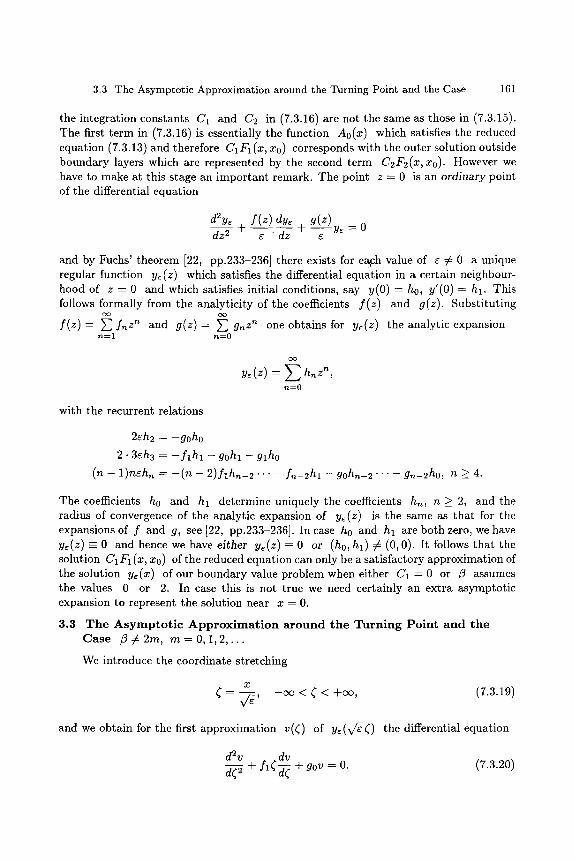
3.3 The Asymptotic Approximation around the Turning Point and the Case 161
the integration constants C1 and C2 in (7.3.16) are not the same as those in (7.3.15). The first term in (7.3.16) is essentially the function Ao(x) which satisfies the reduced equation (7.3.13) and therefore C1Fl(x , xo) corresponds with the outer solution outside boundary layers which are represented by the second term C2F2(x, xo). However we have to make at this stage an impor tant remark. The point z = 0 is an ordinary point of the differential equation
d2y~ f ( z ) dy~ §
dz 2 e dz + g(Z) yE = 0
and by Fuchs' theorem [22, pp.233-236] there exists for e ~ h value of ~ # 0 a unique regular function y~(z) which satisfies the differential equation in a certain neighbour- hood of z - 0 and which satisfies initial conditions, say y(0) = h0, y'(0) = hi. This follows formally from the analyticity of the coefficients f ( z ) and g(z). Substi tut ing
o o
f (z) = ~ f n z n and g(z) = ~ gnz ~ one obtains for ye(z) the analytic expansion n----1 n - - O
o o
n--O
with the recurrent relations
2r = -goho
2.3eh3 = - f l h l - gohl - glho
(n - 1)nehn = - ( n - 2) f lhn -2 . . . . f ,~-2hl - gohn-2 . . . . gn-2ho, n > 4.
The coefficients h0 and hi determine uniquely the coefficients hn, n >_ 2, and the radius of convergence of the analytic expansion of y~(z) is the same as tha t for the expansions of f and g, see [22, pp.233-236]. In case h0 and hi are both zero, we have y~(z) - 0 and hence we have either y~(z) - 0 or (h0, hi) # (0, 0). It follows tha t the solution C1F1 (x, xo) of the reduced equation can only be a satisfactory approximation of the solution y~(x) of our boundary value problem when either C 1 - 0 or fl assumes the values 0 or 2. In case this is not true we need certainly an extra asymptotic expansion to represent the solution near x - 0.
3.3 The Asymptot ic Approximation around the Turning Point and the C a s e ~=/=2m, m = 0 , 1 , 2 , . . .
We introduce the coordinate stretching
X -- - c r < ( < +cr (7.3.19)
and we obtain for the first approximation v(~) of y~(x/~ ~) the differential equation
d2v dv + f l(-;-; + gov = O. (7.3.20) d~ 2 at,
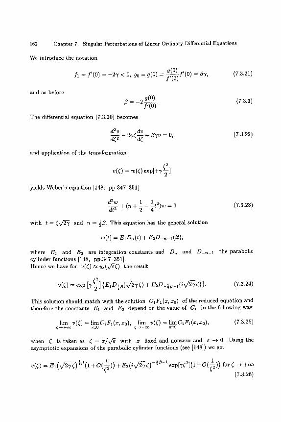
162 Chapter 7. Singular Perturbations of Linear Ordinary Differential Equations
We introduce the notation
g(o) f l = f ' (O) = -27) ' < O, go = g(O) = f ,(O i y ' (o) = / 3 7 , (7.3.21)
and as before
/3= - 2 ~
The differential equation (7.3.20) becomes
g(o) f'(O)"
(7.3.3)
d2~)
d~ 2 dv
- 2 . ~ = + Z.yv = o, a(,
(7.3.22)
and application of the transformation
~2 v(C) = w(~) exp[+7-~-]
yields Weber's equation [148, pp.347-351]
d2w 1 lt2)w = 0 (7.3.23) dt 2 + (n + -~ - -~
with t = ( v / ~ and n = �89 This equation has the general solution
w(t) = E:Dn(t) + E2D_n_:(it),
where E: and E2 are integration constants and D,~ and D-n-1 the parabolic cylinder functions [148, pp.347-351]. Hence we have for v(() ~ y~(v/e() the result
(j-2 v(r = exp [7-~-] { E : D � 8 9 ) + E 2 D _ � 8 9 }. (7.3.24)
This solution should match with the solution C:F1 (x, x0) of the reduced equation and therefore the constants E1 and E2 depend on the value of C1 in the following way
lim v ( ( ) = l imC:Fl(x, xo), lim v(~) = limCiFl(X, Xo), (7.3.25)
when ~ is taken as ~ = x/x/~ with x fixed and nonzero and r -+ 0. Using the asymptotic expansions of the parabolic cylinder functions (see [148]) we get
' I ) -�89 v(:) : E: (X /~ : ) : t 3 (1 + O(~-ff ) + E2 ( i x / ~ : ) exp[7C2] (1 + O ( , _ )) for : -+ +cr
(7.3.26)
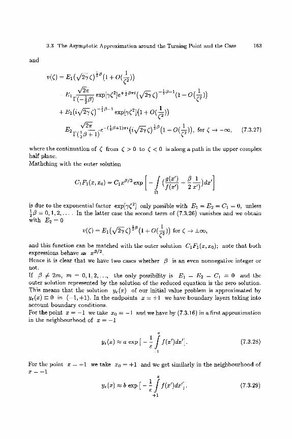
3.3 The Asymptotic Approximation around the Turning Point and the Case 163
and
1 1 v(~) = E I ( ~ - ~ ) 5/3(1 + O(~-~))
- E1F(-I~/3) exp [7~2]e+ �89189 + O ( ) )
1 1 + E2 ( i x / ~ ) - 5 / 3 - 1 exp[~2] (1 + O(~-~))
- E2 P(~/3"x/c~+ 1) e-(�89 ( i V a n ) �89 (1 + O(~-~ff)) , for ~ - -+-00, (7.3.27)
where the continuation of 4 from 4 > 0 to 4 < 0 is along a pa th in the upper complex half plane. Mathching with the outer solution
/ g(x') /3 1 C1F l(x, xo) - C1 x~/2 exp - ( I ( x ' ) + 2 x'---) )dx'
f~
is due to the exponential factor exp[-y~ 2] only possible with E1 -- E2 = 61 = 0, unless �89 = 0, 1, 2, . . . . In the lat ter case the second term of (7.3.26) vanishes and we obtain with E2 = 0
v(~) = E I ( X / ~ ) �89 + O(~-~)) for ~ ~ • , 4
and this function can be matched with the outer solution C1Fl(X, Xo); note tha t both expressions behave as x ~12. Hence it is clear tha t we have two cases whether /3 is an even nonnegative integer or not. If /3 ~- 2m, m = 0, 1 ,2 , . . . , the only possibility is E1 = E2 = C1 -- 0 and the outer solution represented by the solution of the reduced equation is the zero solution. This means that the solution y~(x) of our initial value problem is approximated by ye(x) = 0 in ( -1 , +1). In the endpoints x = +1 we have boundary layers taking into account boundary conditions. For the point x = - 1 we take x0 = - 1 and we have by (7.3.16) in a first approximation in the neighbourhood of x = - 1
X
1 / f(x')dx']. M ys(x) ~ a e x p [ - - e -1
(7.3.28)
For the point x - +1 we take x0 - +1 and we get similarly in the neighbourhood of x = + l
X
1 / f(x')dx'] (7.3.29) b exp[- 7 +1
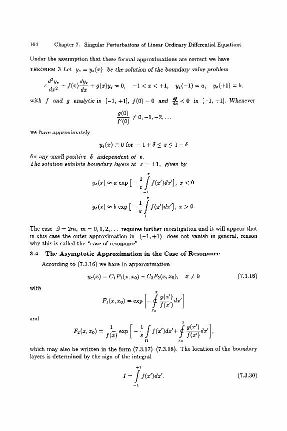
164 Chapter 7. Singular Perturbations of Linear Ordinary Differential Equations
Under the assumption that these formal approximations are correct we have
THEOREM 3 Let y~ = ye(x) be the solution of the boundary value problem
d2ys dye e-~x 2 + f(x)-d-~x + g(x)y~ = O, - l < x < + l , y ~ ( - 1 ) = a , y e ( + l ) = b ,
with f and g analytic in [-1, +1], f ( 0 ) = 0 and ~ < 0 in [-1, +1]. Whenever
g(0) r 0 , - 1 , - 2 , . . . y,(0)
we have approximately
y~(x) =_0 for - 1 + 5 <__ x < 1 - 5
for any small positive 5 independent of e. The solution exhibits boundary layers at x = 4-1, given by
f(x')dx'], x < 0 1
t a r
- - 1
x
1 f y(~' )d~' ] , �9 > o.
1
The case 13 - 2m, m = 0, 1, 2 , . . . requires further investigation and it will appear that in this case the outer approximation in ( -1 , +1) does not vanish in general, reason why this is called the "case of resonance".
3.4 The A s y m p t o t i c Approx imat ion in the Case of Resonance
According to (7.3.16) we have in apparoximation
ye(x) -- CiFl(X, Xo) --b C2F2(x, xo),
with
and
x ~= 0 (7.3.16)
] g(x')dx, F1 (x, xo) = exp - )'(x')
ago
F2(x, xo) = ~ - ~ exp - -e f (xt)dxt + f (x') dxt ,
x o
which may also be written in the form (7.3.17)-(7.3.18). The location of the boundary layers is determined by the sign of the integral
+1
I = f f(x ')dx' . (7.3.30)
- -1
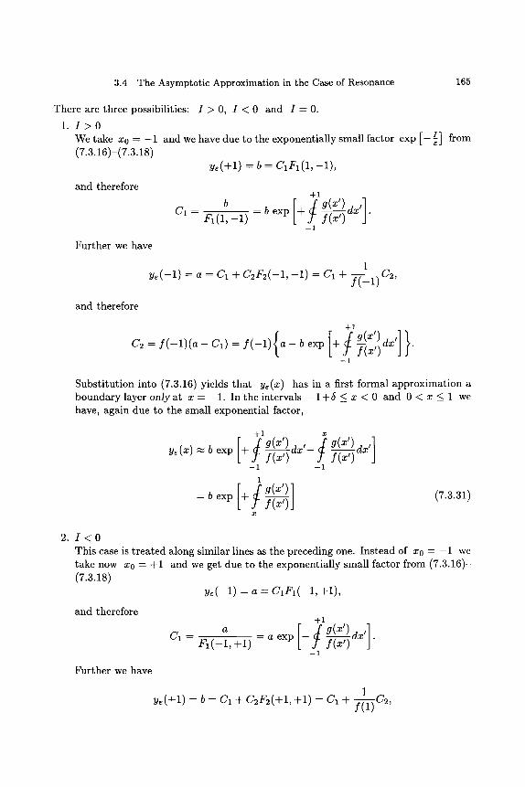
3.4 The Asymptotic Approximation in the Case of Resonance 165
There are three possibilities: I > 0, I < 0 and I - 0.
1. I > 0 I We take x0 = - 1 and we have due to the exponent ia l ly small factor exp [ - ~ ] f rom
(7.3.16)-(7.3.18) y s ( + l ) = b= C1FI(1,-1),
and therefore
Fur the r we have
b C1 = F 1 ( 1 , - 1 )
-I-1
=b dx,] exp f(x') "
- 1
1 y ~ ( - 1 ) = a - - C 1 + C 2 F 2 ( - 1 , - 1 ) = C 1 nt- j~, )~':--1' C2~
and therefore
C 2 - : ( - 1 ) ( a - C l ) - f ( - 1 ) { a - b e x p [ - t - +~Jg(xt)dx'l} f(x')
--I
Subs t i tu t ion into (7.3.16) yields t h a t y~(x) has in a first formal app rox ima t ion a b o u n d a r y layer only at x = - 1 . In the intervals - 1 + 5 < x < 0 and 0 < x _ 1 we have, again due to the small exponent ia l factor,
,i ] [ ,Ix,ldx, ye(x) ,~ b exp + f(z ') f(X')
--1 --1
1
= b exp f(x') ] x
(7.3.31)
2. I < 0 This case is t r ea t ed along similar lines as the preceding one. Ins tead of x0 - - 1 we take now x0 - +1 and we get due to the exponent ia l ly small factor f rom (7.3.16)- (7.3.18)
ye(--1) = a = C1FI(-1, +I),
and therefore
Fur the r we have
-t-1
a [ / ' l x l d x , C 1 = F 1 ( - 1 , +1) = a exp - f(x')
- 1
1 y ~ ( + l ) - b - C 1 --t- C2F2(+1 , +1) - C 1 -t- ~77-:i-~ ~ C2, l~l)
166 Chapter 7. Singular Perturbations of Linear Ordinary Differential Equations
which gives +1
C2= f ( 1 ) { b - a e x p [ - / f ( x , ) �9 --1
The result is a boundary layer term at x = 4-1 and in the intervals - 1 < x < 0 and 0 < x < 1 - 5 we obtain
=aexp I ye(x) = C1 exp -- f(x') ~ J" +1 -1
(7.3.32)
3. I = 0 Inspection of the second te rm in (7.3.16) gives the possibility of two boundary layers, as well in the neighbourhood of x - - 1 as in the neighbourhood of x - +1. We take x0 = - 1 and we subst i tu te the boundary values into (7.3.16) to get a simple system for the integration constants C1 and (5'2. (The choice x0 : +1 leads to the same result for y~(x) ). We obtain
a = C I F I ( - 1 , - 1 ) + C 2 F 2 ( - 1 , - 1 ) = C1 +
b = C 1 F 1 ( + 1 , - 1 ) + C 2 F 2 ( + 1 , - 1 )
1 C2
f ( - 1 )
and therefore
and
af(-1)F2(+l , -1) - b C1 = f ( - 1 ) F 2 ( + 1 , - 1 ) - F 1 ( + 1 , - 1 )
(7.3.33)
b-aFl(+l,-1) (7.3.34) (72 = f ( - 1 ) f ( - 1 ) F 2 ( + l , - 1 ) - F I ( + I , - 1 ) "
Inserting these results into (7.3.16) gives the approximation of ye(x) in the intervals - 1 < x < 0 and 0 < x _ < + l .
After this formal construct ion for the cases I > 0, I < 0 and I = 0, which are formally valid outside the interior layer around x - 0, we have still to investigate the possibility of the matching between the outer solution and this interior layer. Therefore we return to the condition (7.3.25) with v(~) given by (7.3.24) with r 2m, m - 0, 1, 2 , . . . . Just as in the case of nonresonance we have to put E2 = 0 and therefore
~2 v(r = E1 exp ( ' r - x - ) D m ( x ~ ~ ) .
However the parabolic cylinder function Dm (z) with m a nonnegative integer reduces to
Din(z) = ( - 1 ) m e [ z2 dm ( ~ ) ~z e_�89 1 e_�88 z (7.3.35) (v~)~
3.4 The Asymptotic Approximation in the Case of Resonance 167
where Hm denotes the Hermite polynomial of degree rn - ~, see [148] and [22]. Hence
1 v( ~) - E1 ( V/-~)m Hm ( v/~ ~) (7.3.36)
and we have for ~ -+ q-c~
ye(v/e~) ~ v(r ~ E I ( V ~ ) m -- E1 x . (7.3.37)
It follows from the outer solution
[ i(g(x' ) ill) ye(x) - C1Fl(x, xo) - C lx ~/2 exp - f (x ' ) + -2--~ dx'
ft tha t the matching between this solution and the interior layer (7.3.36) is indeed possible with
E 1 - - C I ( ~ ) ~/2 ] ( ) exp - g(x') ~ 1 f (x') + -2-~ dx' . (7.3.38)
xo Moreover the behaviour of ye(x), in the neighbourhood of x = 0, is tha t of a Hermite polynomial which satisfies Fuchs' theorem: in case ye(x) is not identical zero it is of the form
ye(x) -- ho + hlx + h2x 2 + ' " ,
with (ho, hi) ~ (0, 0). Under the assumption tha t our formal constructions are justified we have the following theorem
T H E O R E M 4 Let y~ = ye(x) be the solution of the boundary value problem
d2ye dye ~-d-~ ~ + f (x)-j-~ + g(x)y~ = O, - l < x < + l , y e ( - 1 ) = a , y e ( + l ) - b ,
with f and g analytic in [ -1 , +1], f ( 0 ) = 0 and T~(x)dY < 0 in [--1, +1]. Whenever
g(o) /'(o) = 0 , - 1 , - 2 , . . .
q-1 we have with 1 = f f ( z ' ) d z ' the following approximations of ys(z)" --1
1. I > O" Be(Z) exhibits a boundary layer in the neighbourhood of x - -1 .
1 [ y~(x) ~ b exp + y(z') dx'
x
-1+51_<x_<-52 , +52_<x_<1,
168 Chapter 7. Singular Perturbations of Linear Ordinary Differential Equations
where 51 and 62 are arbitrarily small positive numbers independent o f e.
2. I < O" y~(x) exhibits a boundary layer in the neighbourhood of x - +1
f (~ , ) , -1
- 1 _ x _ - 6 2 , + 6 2 _ x _ < 1 - 6 1 .
3. I = 0 : ye(x) exhibits boundary layers in the neighbourhood of as well x = - 1 as x = + l . The approximation outside -62 < x < +62 is given by (7.3.16) and (7.3.33)- (7.3.34). In all three cases there exists a matching interior layer around x = 0 and it is given by
v(() = E l ( x / 2 ) - m H m ( x / ~ ( ) ,
x 1 , ~ -- 7, (0) and H,~ the Hermite polynomial with ( = ~ , 7 = - ~ f ( O ) , m = 2 - - - (o) of degree m.
3.5 T h e T u r n i n g P o i n t P r o b l e m w i t h i f ( x ) > 0
Because this case is not so interesting as the one with i f ( x ) < 0 we restrict our discussion to the most simple case
d2ye dye e ~ + 2 a x ~ - a f l y e = O , - 1 < x < + l , a > O (7.3.39)
with the boundary conditions
y~( -1) = a, y e ( + l ) = b. (7.3.40)
As in subsection 3.3 we use the subst i tu t ion
[ OtX2 ] u = y~(x)exp ~ ~ , (7.3.41)
which leads again to Weber 's equat ion
d2u
dt 2
1 t 2 + (~ + ~ - ~ ) ~ = 0, (7.3.42)
where t = ~ / - ~ x and n - - l - 2" Similarly as in (7.3.24) we obtain
(~x 2 (7.3.43)
3.5 The Turning Point Problem with f'(x) > 0 169
where D~/2 and D-1-~/2 denote the parabolic cylinder functions and where the integration constants C1 and C2 are to be determined by the boundary conditions (7.3.40). There results
C1 - exp [~-~c ]Ol { a D ~ / 2 ( i ~ ) - A b D f l / 2 ( - i ~ ) } ,
and
with
[26 ] aD_l_,/2( 2o~ ) _ bD_l_, /2(- ) C2 - - e x p
A
: /X D_I_~/2( ~ ~ ) D ~ / 2 ( i ~ ~ ) D_I_~/2(+ ) D ~ / 2 ( i ~ ~ ) (7.3.44)
To calculate the approximation of ys(x) for e $ 0 we need again the asymptotic expansions of the parabolic cylinder functions, [148, pp.347-348]
~z 2 1 )) l argz] < 3/47r D,~(z) - e-Z zn(1 +O(z-- 5 ,
and
1 Dn(z) - e-�88 z'~(1 + 0(---~)) v~ e+'~'rie�88 + 0(~2) ) (7.3.45)
r(-~)
1 and + 5 for argz between 4-~7r ~Tr. Inserting these asymptotic expressions into (7.3.43) we should distinguish between the cases ~ r and ~ = - 2 m , m = 1 , 2 , . . . .
i) The case ~ r m = l , 2 , . . . From (7.3.44) and (7.3.45)we get
{ - ' ~--~--] D- l -~ /2 ( - ) (a - (-1)~/2b)(1 + 0(6)) C1 (6) -- exp [26.1
and
C2(6) = exp [~6] V~/2(i ) b(1 + 0(6)). (7.3.46)
Putting this result into (7.3.43) and using again (7.3.45) we obtain after a tedious calculation:
ye(x) = a(-x) ~/2(1 + O(e)), -1 _< x <_ -5 (7.3.47)
and y~(x) = bx~/2(1 + 0(6)), +5 _< x _< +1, (7.3.48)
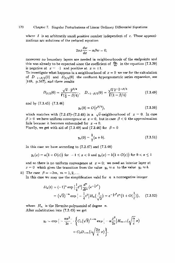
170 Chapter 7. Singular Perturbations of Linear Ordinary Differential Equations
where 5 is an arb i t ra r i ly small posit ive number independent of e. These approxi- mat ions are solutions of the reduced equat ion
dw 2~X-~x a ~ w = 0;
moreover no bounda ry layers are needed in ne ighbourhoods of the endpoints and this was a l ready to be expected since the coefficient of d_~ in the equa t ion (7.3.39) dx is negat ive at x -- --1 and posit ive at x = +1. To invest igate what happens in a ne ighbourhood of x = 0 we use for the calculat ion of D- l - t~ /2 (0 ) and D~/2(0) the confluent hypergeometr ic series expansion, see [148, p.347], and there results
v~" 2 ~/4 (7.3.49) D~/2(0) = 1~{~ -:_ ~-]-~), D_,_~/2(0) : v/~r(12-�89 f~/4)
and by (7.3.45)-(7.3.46) y~(0) = o ( ~ / 4 ) , (7.3.50)
which matches with (7 .3 .47) - (7 .3 .48) in a v~ -ne ighbourhood of x = 0. In case /~ > 0 we have uniform convergence at x : 0, but in case fl < 0 the approx imat ion fails because it becomes unbounded for x -+ 0. Finally, we get with aid of (7.3.49) and (7.3.46) for f~ = 0
1 (a + b) (7.3.51) y~(0) = ~
In this case we have according to (7.3.47) and (7.3.48)
y~(x) = a(1 + O(~)) for - 1 _< x < 0 and y~(x) - b(1 + 0 ( 6 ) ) for 0 < x _< 1
and so there is no uniform convergence at x = 0; we need an interior layer at x = 0 which gives the t rans i t ion from the value ye ~ a to the value ye ~ b.
ii) The case /3 = - 2 m , m = 1 , 2 , . . . In this case we may use the simplif ication valid for n a nonnegat ive integer
1 d" ~ t2 D~(t) = ( - 1 ) '~ exp [~t 2] d -~ (e -~ )
-~ 1 (_~ _lt2t~ O(1 = ( v ~ ) e x p [ - t2]H, t ) = e (1 + ~) ) , (7.3.52)
where H , is the Hermi te -po lynomia l of degree n. After subs t i tu t ion into (7.3.43) we get
c~x21 . { x 2 Ye : exp [ - - - ~ j CI(V/2) I-m exp [-- o~-~E]Hm_I( x)
+ C 2 D - m ( i v ~ x) }"
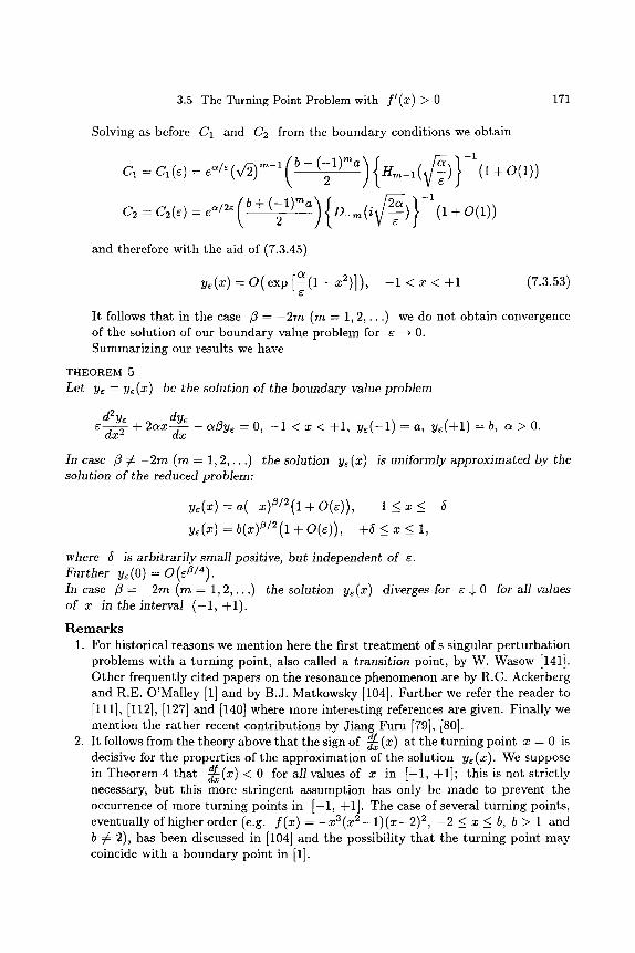
3.5 The Turning Point Problem with f ' (x) > 0 171
Solving as before C1 and C2 from the boundary conditions we obtain
C l = C l ( r 1 7 6 Hm-1( )
C 2 = C 2 ( r { f ~ ) } -1 2 D_m(i ( 1 + O ( 1 ) )
and therefore with the aid of (7.3.45)
y~(x) = O(exp [a(1 - x2)]), - 1 < x < +1 (7.3.53)
It follows that in the case f l - - 2 m (m = 1, 2 , . . . ) we do not obtain convergence of the solution of our boundary value problem for ~ --+ 0. Summarizing our results we have
THEOREM 5
Let y~ - y~(x) be the solution of the boundary value problem
d2y~ dye c ~ + 2aX-d~ x - a~ye = 0, --1 < x < +1, y~(--1) = a, y~(+l) = b, a > 0.
In case 13 ~ - 2 m (rn -- 1, 2, . . . ) the solution ye(x) is uniformly approximated by the solution of the reduced problem:
y~(x) = a(-x)~/2(1 + O(e)), -1 <_ x <_ -5
y~(x) = b(x)~/2(1 + 0(~)), +5 < x < 1,
where 5 is arbitrarily small positive, but independent of e. Further yr = O(~fl/4). In case ~ = - 2 m ( m - 1, 2,. . .) the solution ye(x) diverges for e $ 0 for all values of x in the interval (-1, +1).
R e m a r k s 1. For historical reasons we mention here the first t reatment of s singular perturbation
problems with a turning point, also called a transition point, by W. Wasow [141]. Other frequently cited papers on the resonance phenomenon are by R.C. Ackerberg and R.E. O'Malley [1] and by B.J. Matkowsky [104]. Further we refer the reader to [111], [112], [127] and [140] where more interesting references are given. Finally we mention the rather recent contributions by Jiang Furu [79], [80].
2. It follows from the theory above that the sign of ~ (x) at the turning point x - 0 is decisive for the properties of the approximation of the solution ye(x). We suppose in Theorem 4 that ~-, (x) < 0 for all values of x in [-1, +1]; this is not strictly necessary, but this more stringent assumption has only be made to prevent the occurrence of more turning points in [-1, +1]. The case of several turning points, eventually ofhigher order (e.g. f (x) = - x 3 ( x 2 - 1 ) ( x - 2 ) 2, - 2 < x < b, b > 1 and b ~: 2), has been discussed in [104] and the possibility that the turning point may coincide with a boundary point in [1].
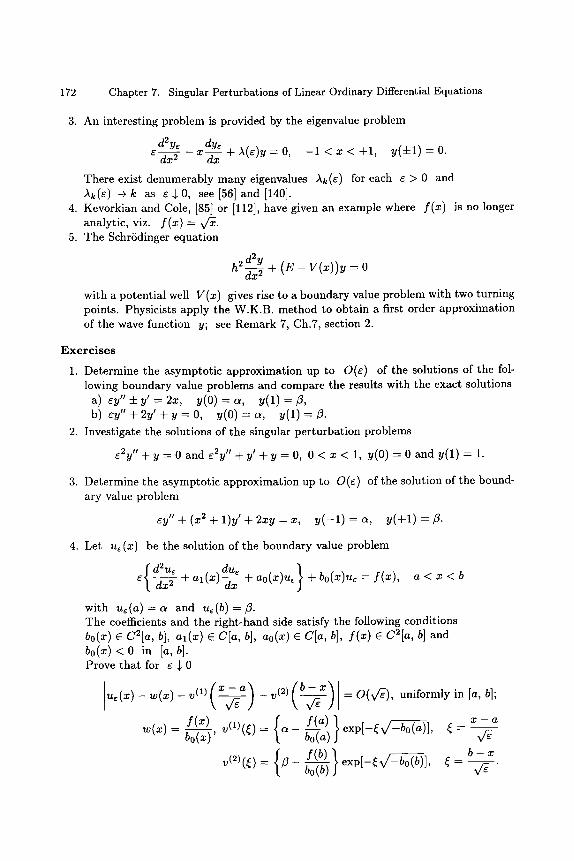
172 Chapter 7. Singular Perturbations of Linear Ordinary Differential Equations
3. An interesting problem is provided by the eigenvalue problem
d2y~ dy~ ~-j~-~ - ~ - ~ - + ~(~)y = 0, - 1 < �9 < +1 , y ( + l ) = 0,
There exist denumerably many eigenvalues )~k(6) for each 6 > 0 and Ak(6) ~ k as 6 ~$ 0, see [56] and [140].
4. Kevorkian and Cole, [85] or [112], have given an example where f(x) is no longer analytic, viz. f ( x ) = vf-x.
5. The Schrhdinger equation
h ~e~yd-~+ (E - r ( x l )y = 0
with a potential well V(x) gives rise to a boundary value problem with two turning points. Physicists apply the W.K.B. method to obtain a first order approximation of the wave function y; see Remark 7, Ch.7, section 2.
Exerc i se s
1. Determine the asymptotic approximation up to 0(r of the solutions of the fol- lowing boundary value problems and compare the results with the exact solutions
a) 6 y " + y ' - 2 x , y ( 0 ) - a , y(1)=/3, b) e y " + 2 y ' + y = O , y ( 0 ) = a , y(1)=fl .
2. Investigate the solutions of the singular perturbation problems
E2y ' ' + y = 0 a n d 6 2 y ' ' + y ' + y = 0 , 0 < x < 1, y ( 0 ) = 0 a n d y ( 1 ) = l .
3. Determine the asymptotic approximation up to 0(6) of the solution of the bound- ary value problem
~y" + ( 2 + 1)y' + 2~y = ~, y ( - 1 ) = ~, y ( + l ) = ~.
4. Let ue(x) be the solution of the boundary value problem
{ d2u~ du~ } 6 ~ + a l ( x ) - ~ x +ao(x)ue +bo(x )ue - f ( x ) , a < x < b
with u~(a)=a and u~(b)= ,6. The coefficients and the right-hand side satisfy the following conditions bo(x) e C2[a, b], el(x) e C[a, b], ao(x) e C[a, b], f(x) e C2[a, b] and bo(x) < 0 in [a,b]. Prove that for r $ 0
l u ~ ( x ) - w ( x ) - v ( 1 ) ( x - a ) - v(2) ( b - x ) vf ~ vf ~ = O(v~), uniformly in [a, b];
s(~) ~(1)(~)= {~_ ~s(~)} w(x) -- bo(x)' exp[_~v/_b0(a) ], ~ = x - a
v(2)(()= 13- b - ~ exp[-(~-bo(b)], ~= b - y e "
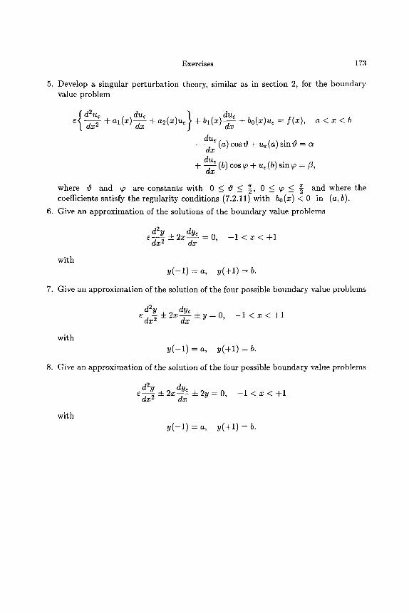
Exercises 173
5. Develop a singular per turba t ion theory, similar as in section 2, for the boundary value problem
{ d2u~ du~ } due ~ + al(x)-d-~x + a2(x)u~ + bl(x)--~x + bo(x)u~ = f(x), a < x < b
due dx (a) cos~9 + ue(a)sin v9 = c~
due + --~-x (b) cos~ + ue(b) sin ~ = fl,
~ and where the where ~) and ~ are constants with 0 G z9 < 5, 0 G ~ G coefficients satisfy the regularity conditions (7.2.11) with bo(x) < 0 in (a, b).
6. Give an approximat ion of the solutions of the boundary value problems
~-~-5x2 + 2x = 0 , - 1 < x < +1
with y ( - 1 ) - a, y ( + l ) -- b.
7. Give an approximat ion of the solution of the four possible boundary value problems
c~-~x 2 • • - 1 < x < +1
with y ( - 1 ) = a, y ( + l ) = b.
8. Give an approximat ion of the solution of the four possible boundary value problems
d2y 6~x2 • 2x 4- 2y = 0, - 1 < x < +1
with y(--1) -- a, y ( + l ) -- b.

This Page Intentionally Left Blank
Chapter 8
S I N G U L A R P E R T U R B A T I O N S O F S E C O N D O R D E R E L L I P T I C T Y P E .
L I N E A R T H E O R Y
1. Introduction
In this chapter we extend the results of the preceding chapter, section 2, to boundary value problems for linear second order partial differential equations of elliptic type. The theory runs largely along the same lines as that for ordinary differential equations. First one constructs a formal approximation satisfying the differential equation and the boundary values up to some positive order of e and consecutively one gives an a priori estimate of the error with the aid of the maximum principle that is also available for partial differential equations of elliptic type. However there are still some complications which arise from the shape of the boundary of the domain of definition. We study the following boundary value problem for the function u~(x, y) defined on a bounded domain ~ C R2:
L~[u~] = eL2[u~] + Ll[u~] = h(x, y), (x, y) �9 ~, (8.1.1)
with
0 2 0 2 0 2 0 L2 = a(x, y)--~x2. + 2b(x, y)OxOy" +c(x, Y )~2 " +d(x, y) Ox
o .+f(~,v) +~(~ ,y )~ .,
and
(8.1.2)
0 L1 . . . . g(x, y), (8.1.3)
Oy
while we have along the boundary 0~t of f~ the first boundary condition
~(~, y)Io~ = ~(~, y)Io~- (8.1.4)
is again a small positive parameter 0 < ~ << 1. To avoid tedious and noninteresting bookkeeping we assume that the coefficients and the right-hand side of the differential
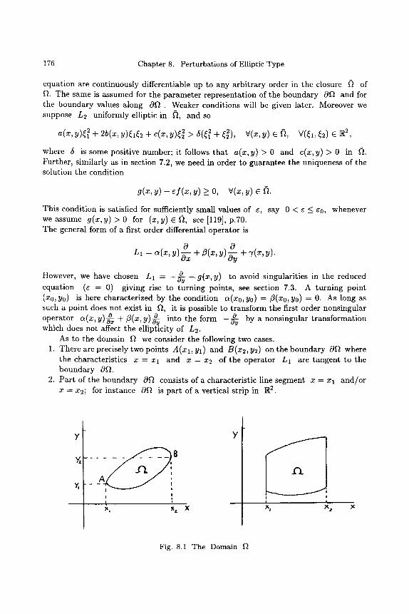
176 Chapter 8. Perturbations of Elliptic Type
equation are continuously differentiable up to any arbitrary order in the closure ~ of f~. The same is assumed for the parameter representation of the boundary 0f~ and for the boundary values along 012 . Weaker conditions will be given later. Moreover we suppose L2 uniformly elliptic in ~, and so
a(x, y)~2 q_ 2b(x, Y)~1~2 + c(x, y)~22 > 5(~ 2 + ~22), V(x, y) �9 ~, V(~I, ~2) �9 R2,
where 5 is some positive number; it follows that a(x, y) > 0 and c(x, y) > 0 in ~. Further, similarly as in section 7.2, we need in order to guarantee the uniqueness of the solution the condition
g(x, y) - ~ f (x, y) ~ 0, V(x,y) � 9
This condition is satisfied for sufficiently small values of e, say 0 < e < e0, whenever we ~ssume g(~ ,y ) > 0 for (~, y) e ~ , see [119], p.70. The general form of a first order differential operator is
0 0 L1 - c~(x, Y)-a-- + ~(x, Y)-_a- + ")'(x, y).
O X ay
o �9 g(x, y) to avoid singularities in the reduced However, we have chosen L1 = 0y
equation (e = 0) giving rise to turning points, see section 7.3. A turning point (x0, Y0) is here characterized by the condition a(xo, Yo) = ,6(xo, Yo) = O. As long as such a point does not exist in ~, it is possible to transform the first order nonsingular operator c~(x, y ) O + fl(x, Y)~u into the form - ~ y by a nonsingular transformation which does not affect the ellipticity of L2.
As to the domain l) we consider the following two cases. 1. There are precisely two points A(x l , Yl) and B(x2, y2) on the boundary 0f~ where
the characteristics x -- X l and x = x2 of the operator L1 are tangent to the boundary 0f~.
2. Part of the boundary 0f~ consists of a characteristic line segment x = Xl and/or x = x2; for instance 012 is part of a vertical strip in R 2.
a !
I I
L X, Xz X
| I
Fig. 8.1 The Domain f~
2. The Maximum Principle for Elliptic Operators 177
These two cases will be treated in this chapter; we make only some remarks for the case that the domain f~ does not satisfy the conditions 1 and 2. In this chapter we present the theory as developed in Ref. [29]. To justify a formal approximation we have to make an estimate of the remainder term; for this we use the maximum principle for elliptic partial differential operators which is t reated in the next section 2. In section 3 we give the formal approximation and in section 4 the a priori estimate of the remainder term and the final results for the case that no part of the boundary 0~t is characteristic. The next section 8.5 is devoted to the second case, where parts of the boundary 0~t may be characteristic. Finally we conclude this chapter with some examples of singularly perturbed elliptic equations with turning points.
2. T h e M a x i m u m P r i n c i p l e for E l l i p t i c O p e r a t o r s
The maximum principle for elliptic operators in two variables may be formulated as follows. Let L be the differential operator
02 02 02 0 0 L = a(x, y)-~x2 + 2b(x, y) OxOy + c(x, y)-ff~u2 + d(x, Y)Ox + e(x, y) Oy
+ f(x, y). := M + f(x , y)., (8.2.1)
elliptic in a bounded domain 7) C R 2 while the coefficients a, b etc. are continuous within 7) with a(x, y) > 0. If a twice continuously differentiable function (I)(x, y) at- tains a local maximum in an interior point P of D then M[(I)] ~ 0 in P. If on the contrary (I) satisfies in 7) the differential inequality M[(I)] > 0 then it follows that
_
(I) cannot at tain a local maximum in 7); if'moreover (I) is also continuous in 7) then the maximum of (I) can only be at tained in some point of the boundary 07) of 7). This is the maximum principle in its most simple form. If the interior local maximum is nonnegative and if f (P) <_ 0 then also L[(I)] _< 0 in P.
P r o o f The proof is very simple since we may always apply an orthogonal transformation in
7) such tha t the value of the coefficient of ~ in P becomes zero. Because we have in
the transformed variables a(&, ~) > 0, c(&, ~) > 0 and ~ < 0, ~ < 0 it is evident b - V - b - ~ - - that the above statement of the maximum principle holds, see also [119], pp.61-68, [23], p.321. [:3
As a corollary of this principle we have again the following useful lemma
LEMMA 1 If the twice continuously differential functions (I)(x, y) and r y) satisfy within a bounded domain 7) the relation
IL[~]I < L [ - ~ ] , V(x,y) e 7), (8.2.2)
where L is the differential operator (8.2.1) with f (x, y) < 0 in 7) and if along the boundary 07) of 7)
I~l __ ~, (8.2.3)
178 Chapter 8. Perturbations of Elliptic Type
then we have also the relation
7"
lr < �9 for all (x, y) e / 7 ) .
0
(8.2.4)
P r o o f : see the proof of Lemma 2 in section 2.2 of Chapter 7.
The function ~ ( x , y ) yields an upper bound for the absolute value of the function
(I)(x, y) in f 7) and so it is called again a barrier function for the function (I)(x, y). 0
A priori est imates of solutions of elliptic boundary value problems may be obtained by constructing suitable barrier functions satisfying the conditions of the lemma. This will be applied later on when we have to give an a priori est imate of the error of the approx- imate formal solution. As in the case of ordinary differential equations the condition (8.2.2) may be replaced by the sharper condition, see [119, Ch.2],
IL[r < L [ - r V(x,y) e D. (8.2.2)*
For a useful application of Lemma 1 we re turn to our boundary value problem (8.1.1)- (8.1.4) with g(x, y) > 0. As to the domain f~ we require in this subsection tha t it is bounded. The regulari ty conditions are more than sufficient to guarantee the existence and uniqueness of the solution, see for instance [23], p.336. A very simple a priori es t imate of ue is given as follows. Since the coefficient e(x, y) is bounded in ~ there exist numbers e0 and a 2 < 1, independent of E such tha t
- 1 + ee(x, y) < - a 2 in fl,
valid for all values of e with 0 < r < e0. Fur ther due to the boundedness of the r ight-hand side h(x, y) and the boundary values ~(x, Y)loa there exists also a number m with the proper ty
Ih( x, Y)I < m in f~
Iq~ x, Y)I < m along 0~.
It is now easily checked tha t the function
m �9 (~, y) = ~ ( y - y0)+ m,
with min y - Y0 is a barrier function for all solutions u~ with 0 < e < r Hence Of~
there exists a number K depending on a and Y0 such tha t
lug( x, Y)I < g m for 0 < e < e0 and (x, y) e ~. (8.2.5)
A much bet ter a priori es t imate is given in the case tha t the shape of the domain is restricted to the cases 1 and 2 mentioned in the preceding section. It can then be shown
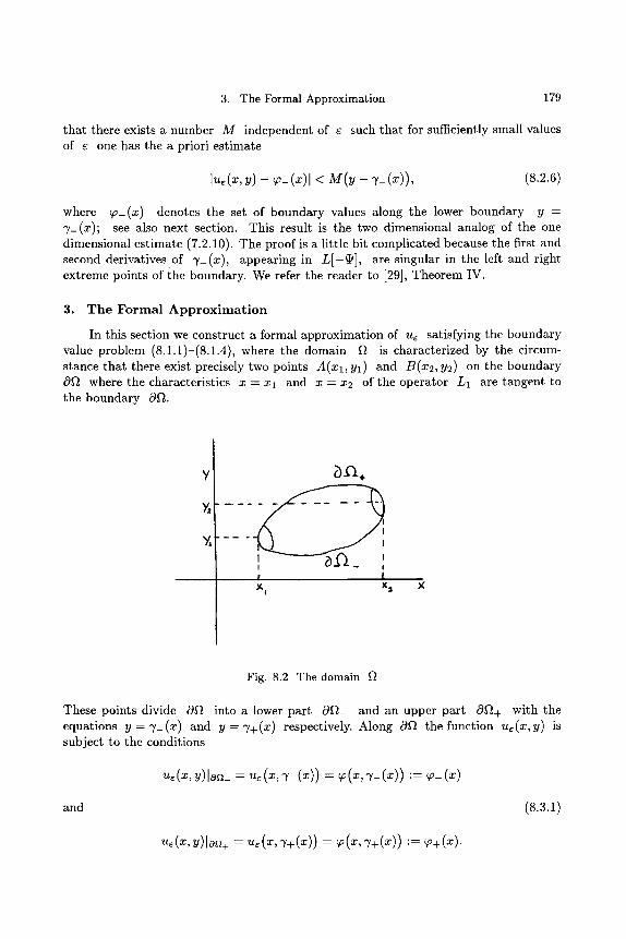
3. The Formal Approximation 179
that there exists a number M independent of ~ such that for sufficiently small values of e one has the a priori estimate
Ju~(x,y) - ~_(x)l < M(y -~/_(x)), (8.2.6)
where V-(x) denotes the set of boundary values along the lower boundary y = ~_(x); see also next section. This result is the two dimensional analog of the one dimensional estimate (7.2.10). The proof is a little bit complicated because the first and second derivatives of ~'_(x), appearing in L [ - ~ ] , are singular in the left and right extreme points of the boundary. We refer the reader to [29], Theorem IV.
3. T h e F o r m a l A p p r o x i m a t i o n
In this section we construct a formal approximation of u~ satisfying the boundary value problem (8.1.1)-(8.1.4), where the domain ~t is characterized by the circum- stance that there exist precisely two points A(Xl, yl) and B(x2, Y2) on the boundary 0~t where the characteristics x - X l and x - x2 of the operator L1 are tangent to the boundary 0~t.
~_O,+
!
. . . . I
r L �9 %~ X2
Fig. 8.2 The domain
These points divide 0~t into a lower part 0gt_ and an upper part 0~t+ with the equations y = ~'_(x) and y = ~,+(x) respectively. Along 0~t the function u~(x,y) is subject to the conditions
u~(~, y).o~_ = u~(~, ~_(~)) = ~(~, ~_(~)) := v_(~)
and (8.3.1)
~ ( ~ , y)to~+ = ~ (~ ,~+(x ) ) = v(~, ~+(~) ) .= v+(~).
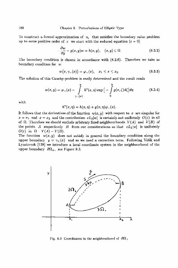
180 Chapter 8. Perturbations of Elliptic Type
To construct a formal approximat ion of ue tha t satisfies the boundary value problem up to some positive order of e we s tar t with the reduced equat ion (6 - 0)
Ow Oy
- ~ - g(x, y)w - h(x, y), (x, y) �9 ft. (8.3.2)
The boundary condit ion is chosen in accordance with (8.2.6). Therefore we take as boundary condit ion for w
~(~ , ~ - ( . ) ) = ~_(~) , ~ < ~ < ~ . (8.3.3)
The solution of this Cauchy-problem is easily determined and the result reads
y Y
,y_ (~1 ,7
(8.3.4)
with h*(~, ~) = h(~, ~) + g(~, ~)~_(~).
It follows tha t the derivatives of the function w(x, y) with respect to x are singular for x = Xl and x = x2 and the contr ibut ion eL2[w] is certainly not uniformly O(e) in all of Ft. Therefore we should exclude arbi t rary fixed neighbourhoods V(A) and V(B) of the points A respectively B from our considerations so tha t eL2[w] is uniformly O(e) in f ~ - V ( A ) - V(B). The function w(x, y) does not satisfy in general the boundary condit ion along the upper boundary y = "7+(x) and so we need a correction term. Following Vi~ik and Lyusternik [138] we introduce a local coordinate sys tem in the neighbourhood of the upper boundary Off+, see Figure 8.3.
~ B
I
A
j ! | i
XI X3,
Fig. 8.3 Coordinates in the neighbourhood of O f +
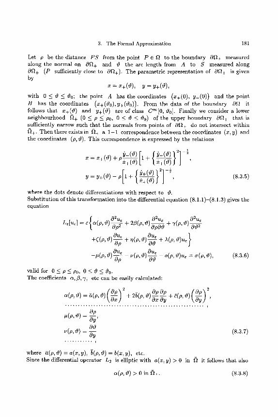
3. The Formal Approximation 181
Let p be the distance PS from the point P C 9t to the boundary 0~t+ measured along the normal on 0~t+ and O the arc length from A to S measured along 0f~+ (P sufficiently close to 0f~+). The parametric representation of 0~t+ is given by
- ~+0), v = v + O ) ,
with 0 _< 0 _< 00; the point A has the coordinates (x+(0), y+(0)) and the point B has the coordinates (x+(tg0),y+(tg0)). From the data of the boundary 0~t it follows that x+(O) and y+(O) are of class C~176 00]. Finally we consider a lower neighbourhood ~+ (0 < p < P0, 0 < 0 < 00) of the upper boundary 0~t+ that is sufficiently narrow such that the normals from points of O~t+ do not intersect within ~+. Then there exists in (~+ a 1-1 correspondence between the coordinates (x, y) and the coordinates (p, 0). This correspondence is expressed by the relations
- ~ + ( o ) + p~+(,9) ~+(,~) '
y= y+(O) - p[l + { il+(o) }z] -�89 &+(0) ' (8.3.5)
where the dots denote differentiations with respect to 0. Substitution of this transformation into the differential equation (8.1.1)-(8.1.3) gives the equation
~ 02u~ O~u~ 02u~ L~[ur - e a(p, O)-~p 2 + 2/3(p, O) + ~,(p, O) OpO0 002
+r 0) Ou~ ou~ } + ~(P' ~)-bY + A(p, ~)u~
_~(p,o)Ou~ Ou~ ~,(p, o) - o(p, O)u~ = ~(p, o) - - - ~ (8.3.6)
valid for 0 < p _ < p 0 , 0 < 0 < 0 0 . The coefficients c~,/3, ~/, etc can be easily calculated"
Oxx + 2b(p, 0) Op Op Op 2 ~ ~ +~(p,~) ~ '
, ( p , o ) = o~' . . . . . . . . . . . . . . . . . . . . . . . . . . . . . . . . . O0
~'(P' e ) = o v (8.3.7)
where ~t(p, O) - a(x, y), b(p, O) = b(x, y), etc. Since the differential operator L2 is elliptic with a(x, y) > 0 in ~t it follows that also
a(p, 0) > 0 in (~+. (8.3.8)
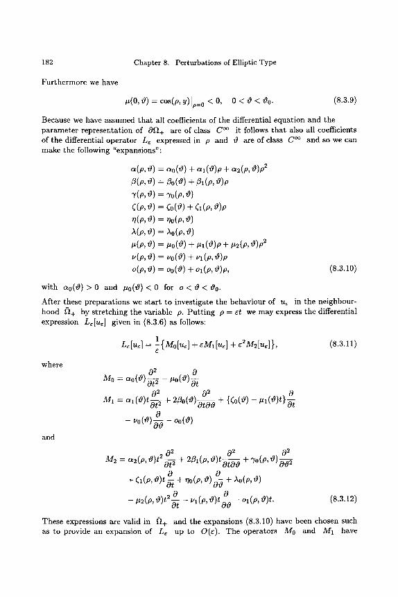
182 Chapter 8. Perturbations of Elliptic Type
Furthermore we have
it(0, 0 ) = cos(p, Y)lp=0 < 0, 0 < 0 < 00. (8.3.9)
Because we have assumed that all coefficients of the differential equation and the parameter representation of 0ft+ are of class C ~ it follows that also all coefficients of the differential operator L~ expressed in p and 0 are of class Coo and so we can make the following "expansions":
a(p, O) = ~o(0) + a l (O)p + a2(p, O)p ~
~(p, O) = ~o(0) + ~ ( p , O)p
"r(;, o) = ~o(;, o)
((p, o) = (o(O) + 6 (p, o)p
n(p, o) = no(p, o) x(p, o) = Xo(p, o)
/.t(p, O) = /.tO(O ) + ~l('bq)P + #2(P, ~9)P 2 .(p. o) = ~,o(.~) + -~(p. ~9)p O(p, O) = O0(t9 ) "[- 01 (p, O)p, (8.3.10)
with ao(O)>O and # 0 ( 0 ) < 0 for o < 0 < 0 0 .
After these preparations we start to investigate the behaviour of u, in the neighbour- hood ft+ by stretching the variable p. Putt ing p = et we may express the differential expression L~[u~] given in (8.3.6) as follows:
where
and
1 {Mo[u~] + eMl[U~] + e2M2[u~]}, Le[u~] -- -~
0 2 0 Mo = ao(O)~-~ - #o(0)~--~
0 2 0 2 0 M1 -- Otl(O)t-~ + 2flo (tg) ~0--~ + {(o(O) -/-/'l(tg)t}~-~
- -o(O) ~ - oo(O)
02 02 0 2 /142 = a2(p, ~)t2~-~2 + 2fit (p, #)t~-D-- ~ + 70(P, ~) O0 2
+ + .o(p, + o(p,
- tt2(p, o ) t 2 0 - ~ l (p , o ) t o , , - o1(p, ~ ) t .
(8.3.11)
These expressions are valid in ~+ and the expansions (8.3.10) have been chosen such as to provide an expansion of L~ up to O(e). The operators M0 and Mi have
(8.3.12)
3. The Formal Approximation 183
coefficients which are linear in t and bounded as functions of 0. The operator M2 has coefficients of the form Xi(p, 0)t ~, i = 0, 1, 2, with X~(P, O) bounded in ~+. The boundary layer term vo(x, y; 6) which should correct the function w(x, y), that satisfies in g t - V ( A ) - V(B) the differential equation up to 0(6) and along the lower boundary 0~t_ the boundary condition us (x, 7 - (x ) ) = ~_ (x), must have the following properties
i) v0(x, y; e) is only defined in the neighbourhood ~t+ of 0~+ and it satisfies the homogeneous equation
02vo Ovo M0[v0] = c~o(0 ) -~ #0(0) - ~ = 0 (8.3.13)
ii) it corrects the boundary condition along 0~t+; hence
{~(~. y)+ ~0(~. y; ~)}[o~+ - {~(p. 9 )+ ~0(p. 9; ~)}1.=0 = ~+ (~+(o))
o r
v0[t=0 = ~+ (x+(0)) - ~(o, O) (8.3.14)
iii) w(x, y)+ vo(x, y; 6) approaches the function w(x, y) as 6 $ 0 for p - 5 ~: 0 with 5 independent of 6; this means
lim vo(t, 0 ) = 0 for 0 < 0 < to0. (8.3.15) t ---~oo
The solution of this boundery value problem is given by
with
P] vo(x,y; 6) = v0(p, 0; 6) = {~+ (x+(0)) - ~(o, 0)} exp [tr
~(o) ,0(~) = < 0 for 0 < 0 < 0o. ~0(o)
(8.3.16)
This function has clearly the character of a boundary layer term; it is asymptotically zero for p ~= 0 with p independent of 6. The two-term w(x, y)+vo(x, y; 6) satisfies in ~t+ the differential equation
Ls[w + v0] - 6L2[w] + h(x, y) + Ml[v0] + 6M2[v0] (8.3.17)
with the boundary condition
(~ + vo)lo~§ - ~§ (8.3.18)
Due to the presence of the term Ml[V0] it follows that Ls[w + vo] - (9(1) uni- formly in ~t+ - V(A) - V(B). To obtain a formal approximation satisfying our boundary value problem up to 0(6) uniformly in ~t+ - V ( A ) - V(B) we still need another term. This is easily done by the addition of an extra boundary layer term 6Vl (x, y; 6) = 6Vl (p, O) = 6Vl (6t, 0), that satisfies in ~+ - V(A) - V(B) the differential equation
Mo[Vl] + Ml[v0] = 0 (8.3.19)
184 Chapter 8. Perturbations of Elliptic Type
with the conditions V 1 (0, b q) - - 0 and lim Vl (t, O) = O.
t - + o o
Due to the exponential behaviour of v0 and the properties of the coefficients of the operators M0 and M1 it is clear that v~ (t, 0) is uniformly bounded in f~+ - V(A) - V(B); v l - - P l ( O , t ) e ~(o)t with P1 a polynomial of degree two in t. Further vl(t,O) is asymptotically zero for p = et =/= 0, because n(0) < 0. Adding the extra boundary layer term eVl we get
with
L~[w + v0 + evl] = eL2[w] + h(x, y) + r + eMl[vl] + e2M2[vl]
= h(x, y ) + O(e), uniformly in ft+ - V(A) - V(B) (8.3.20)
(~ + vo + ~,1)1o,+ = ~'+ (~)"
To obtain a formal approximation of ue in all of f~ - V ( A ) - V(B) we have to extend the relation (8.3.20) outside ~+ - V(A) - V(B) . This is accomplished by introducing the infinitely differentiable cutoff factor r with the properties
1 1 for 0 < p < 5Po
~ p 0 / 0 for 2 5Po ~- P ~- Po,
and by the definition
v i ( ~ , y ; e ) = , ; e ' ' i = 0 , 1 .
Now we consider the expression
u; (~, y) = ~ (~ , y) + .~ (~, y; ~) + ~ (~, y; ~). (8.3.21)
Applying L~ we get in f l - V ( A ) - V(B)
L~[u*~(x,y)] = h(x,y) + eL2[w] + L~[v~ + ev~]
= h(x, y) + eL2[w] + Le[r + eCVl]
= h(x,y) + eL2[w] + e- lMo[r + eCvl]
+ Ml[r + eCvl] + ~M2[r + ecru]
= h(x, y )+ eL2[w] + r + eVl] + Ml[VO + eVl]
+ eM2[vo + r + O(e N)
= h(x, y) + r + O(e) + O(eN), (8.3.22)
uniformly in fl - V (A) - V(B). The symbol O(e N) denotes asymptotically zero. This result follows from the fact that the derivatives of the e independent function r are only nonzero for
4. Estimation of the Remainder Term and Final Results 185
2 l po < P < 5Po, but because v0 and vl are both asymptotically zero for p ~= 0 (p independent of c) we may collect all terms which contain a derivative of r under the symbol o(cg). Summarizing we have
L~[u*~] = h(x, y) + O(e), uniformly in gt - V(A) - V(B), (8.3.23)
with the conditions
u~ It+ : ~o+ (x), (8.3.24)
where F+ are the parts of 09t+ that bounds the region 9 t - V(A) - V(B), while V(A) and V(B) are arbitrarily small, but e independent neighbourhood of the points A and B. The function u~ is a formal approximation of the solution ue of our boundary value problem (8.1.1)-(8.1.4). To show that u* is really a good approximation we consider the remainder Re(x, y) defined as
R~(~, y) = ~ ( ~ , y) - ~; (~, y)
= u~(~, y) - ~ ( ~ , y) - ~ (~, y; ~) - ~ (~, y; ~). (8.3.25)
This remainder term satisfies the conditions
Le[Re(x, y)] = O(e), uniformly in ~ t - V ( A ) - V(B) (8.3.26)
with the boundary conditions Re[r + = 0. (8.3.27)
Moreover Re is uniformly bounded along the right and the left boundaries of V(A) re- spectively V(B) lying in ~t. This latter s tatement follows from the uniform bounded- ness of ue (see (8.2.5))and of u;. These conditions are sufficient for the proof that R~ is indeed O(e) uniformly in
- V ( A ) - V(B). This will be shown in the next section.
4. E s t i m a t i o n of t h e R e m a i n d e r T e r m and F ina l R e s u l t s
First we specify the neighbourhoods V(A) and V(B) of the extremal points A(xl,yl) and B(x2, Y2), see Figure 8.2. V(A) is chosen as the set {(x,y); (xl < x < x l + 5 ) Ngt} and V(B) as the set {(x, y); ( x 2 - 5 < x < x2)A Ft}, with 5 arbitrarily small positive, but independent of e. The remainder Re (8.3.25) is defined in the domain ~ t - V ( A ) - V(B) and it satisfies the boundary value problem:
Le[Re] = O(e), uniformly in ~ t - V ( A ) - V(B),
R ~ ( ~ , ~ _ ( ~ ) ) - o, ~ + ~ < �9 < ~ - ~, R~(~, ~ + ( ~ ) ) = 0, ~ + ~ < ~ _< ~2 - ~,
(8.4.1)
(8.4.2)
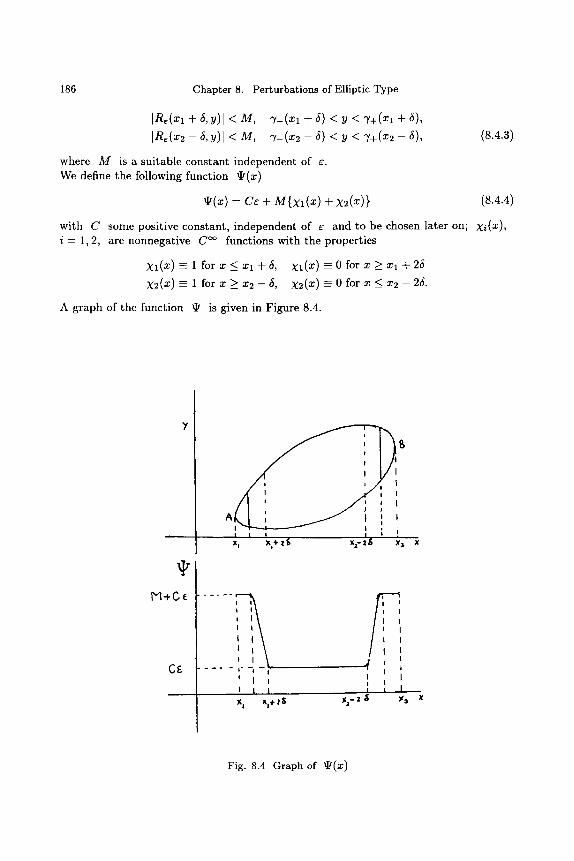
186 Chapter 8. Perturbations of Elliptic Type
In~(x~ + ~,y)l < M, ~-(Xl + 5) < y < ~+(xl + 5),
IR~(x2- ~,y)l < M, "y_(x2- 5) < y < ~ + ( x 2 - 5), (8.4.3)
where M is a suitable constant independent of ~. We define the following function ~(x)
~(x) = C-c --F- M{XI(X)-t- X2(X)} (8.4.4)
with C some positive constant, independent of e and to be chosen later on; Xi(x), i - 1, 2, are nonnegative C ~ functions with the properties
X l ( x ) = l f o r x _ < x l + 5 , X l ( X ) - = 0 f o r x > - x l + 2 5
X2(x) - 1 for x _ x2 - 5, X2(x) -= 0 for x < x2 - 25.
A graph of the function ~ is given in Figure 8.4.
D'I,C ~
C~
i I i I
x , X , § I S X ~ - - I S X ; x
i I I i i I I I I I i i
! i t X i x~+ ~ 8
I I i I I I i I i I
i i j i
, i I J I
i I j l j - 2 $ ~'~ X
Fig. 8.4 Graph of ~(x)
4. Estimation of the Remainder Term and Final Results 187
It follows tha t
Le[-~] = -eM{a(x,y)(x~ t + X~) + d(x,y)(xi + X~2) + f (x ,y) (xz + X2)}
+ Mg(x, Y)(Xl § X2) § cC(-c f (x , y) § g(x, y)).
The order relation (8.4.1) implies the existence of a constant K independent of c such tha t for c sufficiently small, say 0 < e < e0
[L~[R~]I < Ke, V(x, y) E F t - V ( A ) - V(B) .
Because all coefficients of L~ and the functions Xi together with their derivatives are uniformly bounded in ft and further g(x, y) > 0 in ft, it is possible to choose C independent of e and sufficiently large such tha t we get for 0 < e < e0 the inequality
L ~ [ - ~ ] > Kc > [L~[R~][. (8.4.5)
Moreover ~ (x ) is positive along OFt+ and OFt_ and
�9 (x) > M for x = x 1 § 5 and x -- x2 - 6. (8.4.6)
Now it follows from (8.4.1)-(8.4.3) and (8.4.5)-(8.4.6) tha t ~ is a barrier function for Re and so we obtain from lemma 1
IR~(x, Y)I _< ~(x) for Xl + 6 ~_ x ~ x2 - 6
and hence
[R~(x, Y)I-< ~(x) for X 1 § 26 _< X _< X2 -- 26
o r
IR~(x, y)[ _< Ce for X 1 § 26 _~ X < X2 - 26. (8.4.7)
Therefore R~(x,y) is O(e) uniformly in the par t ~* of ~ which is bounded by the verticals x - Xl + 26 abd x - x2 - 26, where 6 is an arbitrarily small positive number independent of e; the same applies to the expression u~(x, y) - w(x, y) - v~ (x, y; e) - ev~ (x, y; e). Finally, because v~ is uniformly bounded in ~* we have also
u~(x, y) = w(x, y) + v 0* (x, y; e) + O(e), uniformly in Ft-*, (8.4.8)
Hence the solution u~(x, y) of the boundary value problem (8.1.1)-(8.1.4) is pointwise approximated uniformly up to O(r in ~t* by the two te rm w(x, y ) § v~ (x, y; e). So we have obtained the following theorem.
T H E O R E M 1
Let u~ be a solution of the boundary value problem (8.1.1)-(8.1.4) with L2 uniformly elliptic in the domain of definition ft, a(x, y) > 0 in ~ and g(x, y) > 0 in ft. The boundary Oft has only two extreme points A and B where the tangent is vertical.
188 Chapter 8. Perturbations of Elliptic Type
Moreover the coefficients and all other data are of class C ~ Under these conditions the solution u~ is uniformly approximated as
u~(~, y) = ~(~, y )+ ~; (~, y; ~) + o(~). (8.4.8)
uniformly valid in a - V(A) - V(B) , where V(A) and V(B) are arbitrarily small e independent neighbourhoods of the points A and B. w(x, y) is a solution of the reduced equation (e = O) and is given by (8.3.4), whereas v~(x, y; e) is a boundary layer term given by (8.3.16) and (8.3.21):
R e m a r k s 1. In case the da ta of the boundary value problem (8.1.1)-(8.1.4) are of class C ~ the
approximat ion (8.4.8) uniformly valid in f ~ - V ( A ) - V (B) may be improved by constructing formal approximations of the form
where
rn r n + l
~; (~, y ) = ~'~,(~, y )+ ~ ~ ,,,.(~, y; ~), i = 0 i=0
m = 1 , 2 , 3 , . . .
Ll[w0] = h(x,y) , wo(x ,v_(x) ) = ~o_(x)
L l [ w i l - - L 2 [ w i _ l ] , wi (x , '~_(x) )=O, i = l , 2 , . . . m .
The boundary layer terms v*(x,y; e) = r e) follow from the expansion of L~ in the boundary layer with coordinates p = et and 0. The expansion is of the form
L~ = e - l { M o -t- e M 1 q- e 2 M 2 -I-" �9 �9 -t- em+lMrn+l} and vi(x, y; e), i - O, 1 , . . . m + 1, are determined by the boundary value problems
M0[v0] = 0, V0loa+ = Volt=o=o = ~o+(x+(v~)) - ~0(0, 0),
lim v0 -- 0, t - -~ o o
i
M0[.,] = - ~ M j [ , , _ j ] , ~ = 1, 2 , . . . ~ , j = l
Viloa+ = vilt=o=o = - ~ i ( 0 , 0), lim vi - 0 t - - ~ o o
and
The final result is
m + l
M0[vm+l] = - E Mj[vm+l- j ] , j = l
Vm+llon+ = Vrn+llt=p=O = 0, lim vm+l = 0. t - - ~ o o
m yr~
e v~ e) + O(e m+l i--0 i = 0
(8.4.9)
4. Estimation of the Remainder Term and Final Results 189
uniformly in F t - V ( A ) - V(B) and valid for all m e {0} U N. For details the reader is referred to [29].
2. It was for reasons of avoiding tedious bookkeeping that we assumed C ~ smoothness of all data of our boundary value problem. However for the validity (8.4.9) it is enough to assume that the coefficients and right-hand side of the differential equation and the boundary values ~+(x) are continuously differentiable up to and including the order (2m + 3) in ~ respectively along OFt. Moreover the parametric representation of OFt. should be continuously differentiable up to and including the order (2m + 6), see [29].
3. The asymptotic expansion constructed above fails in the neighbourhoods V(A) and V(B) of the extremal points. Several authors [138], [53] studied the behaviour of the solution ue(x, y) in these neighbourhoods. To obtain an approximation uniformly valid in the whole domain ~ is rather complicated and involves matching of the approximation in Ft - V(A) - V(B) with that in V(A) or V(B). A result rather easily to formulate has been given by J. Frankena in [42]. In case the boundary OFt in the neighbourhood of A is represented by lY - Yll = 611 x - xll ~/p and in the neighbourhood of B by lY-Y21 = C21x-x21 ~/q with p and q integers not less than 2, the remainder term
R~(~, y) = u~(~, y) - ~ ( ~ , y) - ~ (~, y),
with w and v~ given by (8.3.4), (8.3.16), (8.3.21), may be estimated uniformly _
in all of Ft. The result reads
IRel _< C m i n { ( x - xl)l/p(x2 - x) 1/q, e(x - xl)(1/P)-2(x2 - x)(1/q)-2}, (8.4.10) _
uniformly in Ft; C is a suitable constant independent of ~. Moreover if s = max(p, q) we have the estimate
Re(x, y) = O(el/28), uniformly in ~. (8.4.11)
An improvement of the estimate (8.4.10) has been given by J. Grasman in [53]. Jiang Furu has constructed in [81] a formal approximation of the solution ue(x, y) in the neighbourhoods V ( A ) a n d V(B), using multiple scales (p,~,l_ig(p,~))), where g is a function of p and ~ to be determined by some boundary value problem.
4. A generalization in the direction of more general domains Ft is possible. The requirement of only two extremal points of OFt may be relaxed. To fix the idea consider for example a region Ft as sketched in Figure 8.5. Applying the same construction as explained in this section one obtains
i) boundary layers along A F and D B which correct the function .w(~)(x,y) de- termined from the reduced equation and the boundary values along AB.
ii) a boundary layer along FC that corrects the function w (2) (x, y) determined from the reduced equation and the boundary values along DC.
iii) a "free" boundary layer along D F which smoothes the discontinuity across D F between the functions w (1) and w (2). One might also study for example the interaction of the three boundary layers in the neighbourhood of the point F. For results see lit.[105], [106].
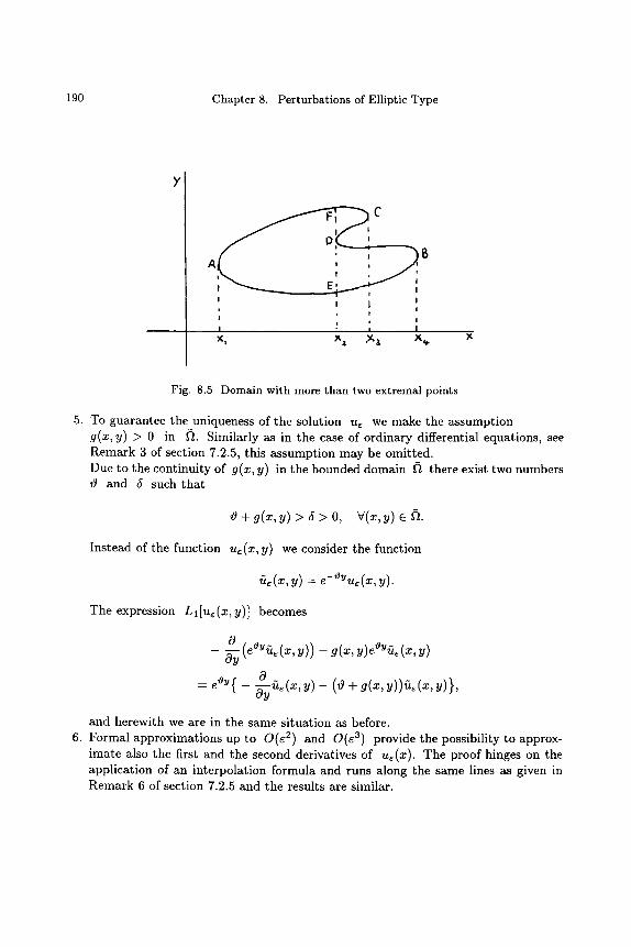
190 Chapter 8. Perturbations of Elliptic Type
B A
I i I
i I
l i I
I " 1 I
Fig. 8.5 Domain with more than two extremal points
5. To guarantee the uniqueness of the solution u~ we make the assumption g(x, y) > 0 in ~. Similarly as in the case of ordinary differential equations, see Remark 3 of section 7.2.5, this assumption may be omitted. Due to the continuity of g(x, y) in the bounded domain ~ there exist two numbers 0 and 5 such tha t
0 + g(~, y) > ~ > 0, v(~, y) e ft.
Instead of the function u~(x, y) we consider the function
~ ( ~ , y) = ~-O~u~(~, y).
The expression Ll[ue(x,y)] becomes
0 Oy (e'~Uue(x' y)) - g(x, y)eaY~e(x, y)
= e ay { - ~ y ~ ( x , y) - (0 + g(x, y))~e(x, y)},
and herewith we are in the same situation as before. 6. Formal approximations up to O(r 2) and O(e 3) provide the possibility to approx-
imate also the first and the second derivatives of u~(x). The proof hinges on the application of an interpolation formula and runs along the same lines as given in Remark 6 of section 7.2.5 and the results are similar.
5.1. Introduction 191
5. D o m a i n s wi th Character i s t ic Boundar ie s
5.1. In troduc t ion
It is of interest to study singular perturbation problems associated with the partial differential equation
Ls[us] = eL2[us] + Ll[us] = h(x, y), (x, y) e a (8.5.1)
with L2 of order 2 and uniformly elliptic in ft and with L1 of order 1, while the boundary 0f~ of the domain ft contains parts which are characteristics of the operator L1. In this section we treat an example to illustrate the procedure for handling problems of this kind; a more general case has been treated by Eckhaus and de Jager in [29]. Before setting up a scheme for the construction of a formal approximation of u~ we study first a simplified problem in order to get some insight into the behaviour of us in the neighbourhood of a characteristic boundary. Therefore we consider the following boundary value problem
{ C')2Ue O2Ue } -'~'- -'~y2 Ls[u~] - e Oy =0, x > 0 , y > 0 (8.5.2)
with
us(x,O)=O, x>_O, us(O,y)=qo(y), y_>O, qo(O)=O, (8.5.3) d 2 where d . . . . . 99, ~yy, and ~ are uniformly bounded; the need of this regularity condition for
qo will become clear later on. The solution w of the reduced equation that satisfies w(x, 0) - 0 is simply w -- 0. This solution does not fulfil the boundary condition us(0, y) = qo(y) and so we need again a correction term. We introduce the local coor- dinate
X
= v~ (8.5.4)
and the equation (8.5.2) is transformed into
02us Ous O~ 2 Oy
0 2 u s = ~ ( 8 . 5 . 5 ) Oy2 "
In this preliminary situation we might expect that a first formal approximation of us is given by the solution of the boundary value problem
02v Ov O~ 2 Oy -- 0 (8.5.6)
with the conditions
v ( ~ , 0 ) = 0 , ~ > 0 a n d v ( 0 , y ) - q o ( y ) , y > 0 .
The solution is easily obtained and it reads
( x )
~ / v ~
(8.5.7)
(8.5.s)
192 Chapter 8. Perturbations of Elliptic Type
Hence 2
tvl < M ~ erf c[ ],
where M is the upper bound of the function I~(Y)]" So v is uniformly bounded and analyzing the expression (8.5.8) for large values of f and finite values of y one gets
X , (~, yo) = o ( ~ ) , (8.5.9)
uniformly for x > 5 > 0 and any fixed value y0 >_ 0. 5 may be any positive number, indpendent of e and the symbol O(e N) denotes again asymptotically zero (see also Exercise 8 of Chapter 2). Therefore the function v ( ~ , y) is a boundary layer function and we call it a parabolic boundary layer function since it is a solution of a parabolic differential equation. We put now
X ~(~, y)= .(~, ~) + R~(~, y),
where Re satisfies the boundary value problem
02 Re 02 R~ ~ ORe 02 v e OX 2 + ) = - ~ y Oy 2 Oy -~y2, x > O, >0
with R~(~, 0 ) = R~(0, y ) = 0, ~ > 0, y >__ 0. (8.5.10)
x O2v To show that v ( ~ , y) is at least a formal approximation of ue(x, y) we need sb--~y2 = o(c), uniformly in x > 0, y >_ 0, or eventually in a bounded part of this region, say x 2 + y2 < r 2. However we have from (8.5.8)
o o
02v V ~ { ~ exp[ 1~2 / �89 2 ~2 } Oy 2 -- (2y)3/2 ~yy]~'(O) + e- ~o"(y- ~-~)at (8.5.11)
~/,/'N
and it follows that ~ ~ has a corner sigularity at the origin x = 0, y = 0 whenever ~'(0) ~= 0. The nature of this singularity is clearly revealed if in equation (8.5.11) the origin is approached along any curve ~ = my ~ with m and c~ arbitrary positive constants. The presence of this corner singularity indicates that in at tempting a proof for an appropriate estimate of the remainder Re we may expect a difficulty. This difficulty disappears whenever dd-~y (0) = 0 and therefore we change the boundary. condition ue(0, y) = ~(y) a little bit such that the new boundary value ~5(y) has the properties ~(0) = 0 and -~y(0) = 0. Therefore we define
~(y) -- ~ ( y ) - y~o'(O)exp[-- Y l, (8.5.12)
5.1. Introduction 193
where a is a positive constant to be determined later on. We have indeed ~(0) = 0 and ~'(0) = 0; moreover the change in the boundary condition is small because
~(y) ~(y) = ~' (0) ~ = - --exp [ - ~ ] O(~),
uniformly for 0 _< y < oo. Instead of the approximation v that satisfies (8.5.6)-(8.5.7) we use now the function
that fulfils (8.5.6) and the boundary conditions
~ ( ( , 0 ) = 0 , ~ > _ O a n d ~ ( O , y ) = ~ ( y ) , y > O .
Similarly as in (8.5.8) we get
oo
~((, y) = e-~ ~(y - - ~ ) d t . (8.5.13)
Assuming ~o"(y) continuous we obtain from substitution of (8.5.12) into (8.15.11)
o~ ~ ~2 2 ,(o)___~. oy~ = ~- r ~ ) + {~-~
dt
~/ v ~ = 0(1) 4- 0 (~-~) , uniformly in any quarter disk x 2 4- y2 < r 2. (8.5.14)
Putt ing now X
ue(x, y) = ~ ( ~ , y) +/~e(x, y), (8.5.15)
we have instead of (8.5.10) for the remainder term /re the boundary value problem
r Ox 2 4. = = . (~y2 (~y --g '~y2 O(~) + o ( ~ l - - a ) , (8 5.16)
uniformly in x 2 + y 2 _ < r 2, with /~e(x, 0 ) - 0 , x_>0 and /~(0, y ) = p ( y ) - ~ ( y ) - 1 and it follows O ( ~ ) , uniformly in y _> 0. The exponent a is still free; we take a =
that ~ ( ~ ) is a formal approximation of ue(x, y).
To prove that ~ ( ~ , y ) is indeed a good approximation of ue (x , y ) we make an estimate _
of / ~ invoking again the maximum principle. A simple barrier function for Re is given by
-= v/~C(1 4- y),
with C sufficientily large and we get
/~ (x , y) - O(x/~), (8.5.17)
uniformly in any bounded domain x 2 + y 2 _ _ r 2, x_>0, y_>0. Hence
X u ~ ( x , y ) = ~ ( ~ , y ) + O ( x / ~ ) , uniformly i n x 2 + y 2 _ _ r 2, x_>0, y_>0.
194 Chapter 8. Perturbations of Elliptic Type
However
(x)
v(~, y) -- ~(~, y) -- 99 (0) e-�89 t2 (y -- ~-~) exp
~/v'~-~
= O(v/e), uniformly in x >_ O, y _> O,
Y - 2t2 dt v~
and so we may finally conclude
X u,(~, y) = v ( -~ , y) + o(v~), (8.5.18)
uniformly in x 2 + y2 <_ r 2, x > O, y >_ O, where v ( ~ , y) is given by (8.5.8).
The boundary layer term 0(~,y) is called a regularized boundary layer term. In a first approximation of ue the nonregularized boundary layer term is sufficient; the regularization is only needed to prove that the error is O(V/r uniformly in any bounded region of the domain x _> 0, y _> 0. Summarizing we have the following theorem
THEOREM 2 ~ continuous Let uE satisfy the boundary value paroblem (8.5.2)-(8.5.3) with qo, du ' dy2 ,
for y > O. Then the solution ue(x, y) is approximated by
oo X V~~ / 1 t 2 x 2
u~(~, y) = v ( ~ , y) - ~-~ ~(y - 2 - ~ ) e t + o ( v~ ) z
uniformly in any bounded region in the domain x > 0, y > 0.
5.2. T h e S i n g u l a r P e r t u r b a t i o n P r o b l e m in a R e c t a n g l e
By now we have carried out sufficient preparations for the t reatment of a singular perturbation problem associated with the differential operator e A - ~ and defined in a rectangle. To be specific we investigate the following boundary value problem
(0 9u~ 02u~ ~ Ou,
r ~ + Oy 2 ] Oy = O, 0 < X < el, 0 < y < s (8.5.19)
with the boundary conditions
Ue(X, 0) : f l (X), 0 < X < el, Ue(X, e 2 ) : f2(x), 0 < X < el,
U,(0, y) -- gl(Y), 0 < V < 12, U,(l l , y) = g2(v), 0 < y < e2, (8.5.20)
where
f l (o ) -- g~(O), f~(e~) - g2(0), f2(0) = g~(e2), f2(e~) - g2(e2).
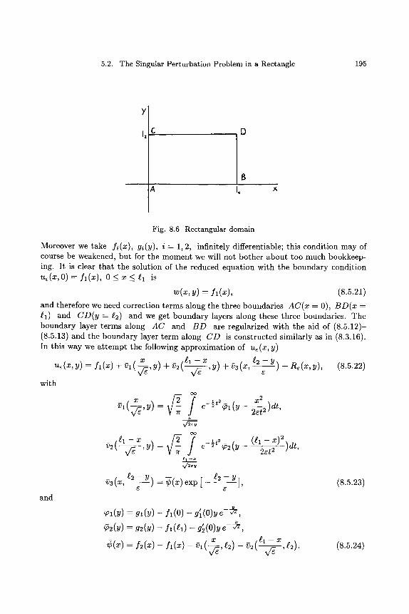
5.2. The Singular Perturbation Problem in a Rectangle 195
Y
. , , .
D
$
Ii
Fig. 8.6 Rectangular domain
Moreover we take f~(x), g~(y), i = 1, 2, infinitely differentiable; this condition may of course be weakened, but for the moment we will not bother about too much bookkeep- ing. It is clear tha t the solution of the reduced equation with the boundary condition ue(x,O) = f1(x), 0 _< x < s is
W(X, y) = fl(X), (8.5.21)
and therefore we need correction terms along the three boundaries AC(x = 0), BD(x = ~1) and CD(y = ~2) and we get boundary layers along these three boundaries. The boundary layer terms along AC and BD are regularized with the aid of (8.5.12)- (8.5.13) and the boundary layer te rm along CD is constructed similarly as in (8.3.16). In this way we a t t empt the following approximat ion of u~(x, y)
( ~ e l ~ - x, y) -~- v3 (x, ~2 c-- y) Jr_ Re(x, y) ue(x, y) = f l (x ) Jr- Vl , y) + 32( ..
with
x x2 Vl(-~,y) -- e-~t ~I(Y-- ~t2) dr,
oo / .1_.2 ~ I - - X y) = e - (~2(Y-- )dt
and ! -- --Y--
(~1 (Y) - - gl (Y) -- f l (0) - gl (O)y e ,/;, _ ,
~2(Y) - g2(Y) - f1(~1) g2(0)Y e ,
- x ~ 1 - x ~ 2 ) .
r - s ~ ( ~ ) - / ~ ( ~ ) - ~1 ( ~ , e ~ ) - ~ ( v~ '
(8.5.22)
(8.5.23)
(8.5.24)
196 Chapter 8. Perturbations of Elliptic Type
From the estimate (8.2.5) or (8.2.6) it is celar that ue(x, y) is uniformly bounded in the rectangle A B e D and so Re(x, y) is also uniformly bounded in this rectangle. Moreover Re(x, y) satisfies the boundary value problem
(0 2Re 02Re ) ORe O X 2 -t- = Se(X, y), 0 < X < el, 0 < y < g2, (8.5.25) Oy 2 Oy
with
and
02el X 02V2 gl --X d2 f l ( x ) ~- ( y) -~- ( , y)
d2r ~2 -- Y] } + ~x2 (x)exp [ -
R~(~, 0) = - ~ ( ~ ) ~ - ~ , R~(~,e2) = 0
gl g2 , _._It_ Re(O,y) = - - v 2 ( ~ , Y ) - - v3(0, e - y) + gl(O)ye ~
gl g2 , -- __.E_
(8.5.26)
(8.5.27)
After careful inspection of the boundary data along the boundary of ABCD, using a.o. (8.5.20), it appears that we have the uniform estimate
R~(~, y) = O(v~). O ( A B C D )
(8.5.28)
To estimate Re(x, y) in the interior of ABCD we have to investigate the right-hand side 1 Se(x, y) of (8.5.25). We have ef~'(x) = O(e) and by means of (8.5.14) with a = ~ we
have also the estimates ~ ~ x ou 2 ( ~ , y ) = O ( v ~ ) and e ~ 2 ~ v~ ' Y ) = O(v~) , uniformly
in ABED, and so it remains to inspect d--~(x)exp[-- ~2-u] in A B e D d x 2 e J "
d2(p _ f ~ , ( x ) _ y I , ( x ) - 1{ 0 2 0 2 } ax 2 - ~ ~12'01(~1, e2) + ~--~'02(~2, e2) , (8.5.29)
where X ~1 -- X
~1= ~ a n d S 2 = V/~ �9
It follows tha t d2 ~ ~ ] = 1 exp [ - e J O(~) and Se(x,y) = O(1) in smallneighbourhoods of the cornerpoints C and D. An estimate of Re(x, y), uniformly small in the whole rectangle ABCD is not yet possible and therefore we improve the boundary correction along the upper side CD. We remark that it is not surprising that we are at this stage not yet ready to give a uniformly small estimate for the remainder term; the
5.2. The Singular Perturbation Problem in a Rectangle 197
reason is the overlap of two boundary layers in the cornerpoints C and D. Using the local coordinate 7/ - e2-v the boundary layer term V3 has been obtained as a first approximation of the boundary value problem
02v * ~2 02v * Ov* _~2 , (8.5.30) - - + = O < x < ~ , O < rl < - - C~?~ 2 OT] OX 2 '
with the boundary conditions
x i l - x v*(x ,O) = (p(x) - f : ( x ) - f~ (x ) - ~ , l ( - - ~ , t 2 ) - ~,~.( V'Z , t~ ) ,
v*(~, ~)- = o .
(8.5.31)
(8.~.32)
- l~ -y The approximation ~3(x, , ) - r = ( p ( x ) e - ~ satisfies (8.5.30) with e = 0 and the first boundary condition (8.5.31), while the second boundary condition is replaced by lira v*(x, 77) - 0. Instead of ~3(x, r/) we take now as an approximation of v*(x , rl) ~-~c~
~(~, ,) + C~(~, , ) ,
where V4(X, 77) is a solution of
~2 02V4 OqV4 -- 02~3 d2r (x)e -~/ 0 < x < ~1, 0 < 71 < - - cOrl 2 ~ (Or I - cox 2 - d x 2 ' ----c '
with the conditions V4(X, O) -- 0 and limn__~ V4(X,?7) -- O, 0 _~ X ~ ~1. It follows immediately that
d25 Vn(X, ?7) "-- ~X277 e-~" (8.5.33)
Finally we decompose the function u~(x , y) as
( ~ ~1 -- X y) - [ -~3(X ' u~(~, y) = f l(~) + ~ ' Y) + ~ ( v~ '
+ k~(~, y).
Now we have obtained for /~e(x, y) the following boudary value problem
02 02 ) 0/~e = 5 ( x , y), (8.5.34)
with
{ '/ 02Vl X 02V2 ~ , l - -X ,y )_ .~_E2d4~) } = ~ f~ (~1 + -~y~(-~' Y) + -~y~( v~ -~,Te-" (8.5.35/
198 Chapter 8. Perturbations of Elliptic Type
and boundary conditions similar to (8.5.27). With the aid of (8.5.24) and the definitions (8.5.23) we have
~4~ = O(e-~) and ~x 4 - O(e-2),
uniformly in A B e D and by means of (8.5.14) with a - 1 we get
Se(x, y) = O(v~), uniformly in A B E D . (8.5.36)
The addition of the boundary values of e2~4(x, y) have changed the boundary values of Re(x, y) only up to O(r 2) and so we have accordingly to (8.5.28)
/~e(x, y ) = O(v~), uniformly along O(ABCD). (8.5.37)
Introducing once again the barrier function
@(x) = Cv/e(y + 1),
with C sufficiently large, but independent of e, we obtain by (8.5.34), (8.5.36), (8.5.37) and Lemma 1 the result /~(x, y ) - O(V~), uniformly in A B E D . Hence
.~_ e2~4(X, g2 - Y) + O(v~), uniformly in A B E D . C
Finally, because V4(X,7/) = d-~-e-ndx, 'i = 0(}) and v,- ~, = O(v~), i= 1,2, see
(8.5.18), uniformly in A B E D , we have also
( ~ ~' - ~ y) + ,~(~, ~ - Y) + O ( v ~ ) ue(x,y) : f l ( x ) - q - ~1 ' Y ) -]- v2( ~ ' c '
uniformly in the closed rectangle A B E D , (8.5.38)
with
oo �9 "{ ' ) VI (--~, Y) - - - e-2 gl (Y -- ~et2 ) -- fl(O) dt,
z
"' ,Y)= "- g . ( Y - 2.t-------~-
(8.5.39)
(8.5.40)
and
~3( x, g2 -- Y) _-- r exp_ [s -- Y], C
(8.5.41)
5.2. The Singular Perturbation Problem in a Rectangle 199
where
x 12) - v2( 12). (8.5.42) - '
Summarizing our results and keeping track of the required differentiability of the data we have established the following result
THEOREM 3 Let the function u~(x, y) be the solution of the boundary value problem
{02u~ 02u~} Ou~
+ -O-yy o y = 0
in the domain 0 < x < s 0 < y < ~2, with 0 < e << 1 and with the boundary conditions
ue (x , O ) - f l ( X ) , Ue(X,~2) -- f2(x) , 0 _~ X _~ ~1,
us(O, y) -- gl (Y), ue(~l, Y) -- g2(Y), 0 _~ y _~ ~2.
Under the assumption that the boundary values are continuous in the cornerpoints (f l (0) = g(O), etc.) and that fi and gi (i = 1, 2) have continuous derivatives up to and including the order four, one has for ue the uniform estimate (8.5.38) given above.
R e m a r k s 1. The boundary value problem treated in this section has been studied also by
L.P. Cook and G.S.S. Ludford [21]. They investigated a semi-infinite strip problem with the aid of Fourier transformation and the results for the rectangle were obtained from the superposition of two infinite strip problems. Further we mention the work by V.A. Nye [110] who studied the boundary value problem with boundary values also dependent on e.
2. The theory of this chapter is useful for the study of the magnetohydrodynamic flow in ducts with a circular or rectangular cross section, see refs [110], [121], [126] and [81] .
3. Another interesting approach to linear singular perturbat ion problems, applicable to as well ordinary as partial differential equations in several variables is due to Y. gana i [83], [84]. The singular perturbation problem for u(x) - u(x: , x 2 , . . . , x,~) is written in the form
L2[u] + AL:[u] = 0, A > 1, x �9 f~, u(x) = 9~(x), x �9 0~2, (8.5.43)
where L2 is an elliptic differential operator of the second order, L: a differential operator of the first order and ft a bounded domain. Applying the Lapace transformation
y
u~ (x) -- / exp[--Ay]v(x, y)dy
0
(8.5.44)
200 Chapter 8. Perturbations of Elliptic Type
one obtains a hyperbolic differential equation
0 L2[v] + -~--Ll[v] = 0, (8.5.45)
ay
valid in the cylinder f l x ]R 1 and with the boundary conditions
v(x, y) = 0, y < 0 and v(x, y) = ~(x)~(y) for y > 0.
Investigating v(x, y), in particular its support, and approaching u~ (x) for -4 c~ with the aid of (8.5.44) one obtains an approximation of the solution of
the singular per turbat ion problem. Y. Kanai treats a.o. the elliptic problem
" 0 �9 +c(~). L2 = Ax and L1 = ~-~bj(x)-~-~. j = l
and the parabolic problem
L2 = / k x and L1 = bj ~x- Ot ' L] 3
j = l
(Ax is the Laplace operator). Further he presents an outline for a simple turning point problem in one dimension. For related work we refer the reader also to L. Frank, Singular Perturbat ions I, North-Holland Publ.Cy, Amsterdam, 1990.
6. Elliptic Boundary Value Problems with Turning Points
6.1. I n t r o d u c t i o n
In the preceding chapter we have studied per turbed boundary value problems for ordinary differential equations of the form
d2ye dye c ~ + f (x)--~x + g(x)y6 = O, - 1 < x < +1, (7.3.1)
where the reduced equation (~ = 0) may become singular due to a turning point, say at x = 0, with f(0) = 0. It appears tha t the approximation of the solution is highly sensitive for the sign of the derivative f~(x) at x = 0 and for the value of the parameter
~ = g(O) (7.3.3) 2 f'(O)"
Phenomena similar as those demonstrated in section 7.3 may of course also occur in the case of partial differential equations of elliptic type. In the next subsection we give some examples, however without entering into the details of rather complicated calculations.
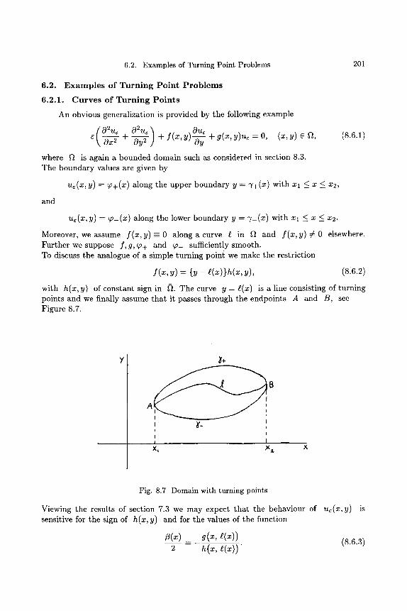
6.2. Examples of Turning Point Problems 201
6.2. E x a m p l e s of T u r n i n g P o i n t P r o b l e m s
6.2.1. C u r v e s of T u r n i n g P o i n t s
An obvious generalization is provided by the following example
0 2u~ 0 2u~ ~ Ou~ ~ + 0y~ / + :(~' Y)-0~-y + 9(~, y ) ~ = 0, (~, y) �9 ~, (8.6.1)
where ~t is again a bounded domain such as considered in section 8.3. The boundary values are given by
ue(x, y) = ~+(x) along the upper boundary y = ~/+(x) with xl _< x < x2,
and
ue(x, y) = T_(x) along the lower boundary y = V_(x) with xl <_ x < x2.
Moreover, we assume f (x , y) - 0 along a curve i in fl and f (x , y) =/= 0 elsewhere. Further we suppose f , g ,~+ and ~_ sufficiently smooth. To discuss the analogue of a simple turning point we make the restriction
f (x , y) = {y - t.(x)}h(x, y), (8:6.2)
with h(z, y) of constant sign in ~t. The curve y - l(x) is a line consisting of turning points and we finally assume that it passes through the endpoints A and B, see Figure 8.7.
8
A t
I !
! _, .,.
X, '~z
Fig. 8.7 Domain with turning points
Viewing the results of section 7.3 we may expect that the behaviour of u~(x, y) is sensitive for the sign of h(x, y) and for the values of the function
~(x---J). = - g ( x ' l(x)) (8.6.3) 2 ~(~, t ( ~ ) )
202 Chapter 8. Perturbations of Elliptic Type
We expect the following i) Similarly as in Theorem 3 of Chapter 7 we have in the case
~ ( '~ h(x, y) < 0 in fi and ~.~x, :/= O, 1, 2 , . . . (8.6.4)
2
the result that ue(x, y) is approximately zero in any e-independent closed interior of f~ and that ur y) is approximated by boundary layer functions along the upper and lower boundary of 12.
ii) Similarly as in Theorem 5 of Chapter 7 we have in the case
h(x, y) > 0 in l~ and fl(x) ~= - 1 , - 2 , . . . (8.6.5) 2
the results
y
~-(~)
"y_(x) <_ y <_ g(x) - 5 (8.6.6)
and
y
"y+(~)
g(x) + 5 <_ y <_ ~+(x), (8.6.7)
where 5 is an arbitrarily small positive number independent of s. In the neighbourhood of the curve y = ~(x) there is a free boundary layer con- necting the approximations (8.6.6)-(8.6.7). This case with g(x, y) - 0 has been worked out in Ref. [76].
6.2.2. Isolated Turning Points; Nodes
We take as our boundary value problem
( 02u~ 02u~] ( Ou~ Ou~ L~ [ u~ ] = e ~ + O Y 2 ] + x -~-~x + y -~y ) = 0 , 0 ~ X 2 -~- y2 < 1
with ue(x, y) - f(cp) for x 2 + y2 _ 1, (8.6.8)
where ~o denotes the polar angle with 0 _< ~o < 21r. Transforming to polar coordinates we get
02ue 10ue L ~ [ u e ] - e ~ + - + - - - - ~--~r
Oue 1 02ue :l=r =0 , r 2 0~0 2
0 _ r < l , 0 < ~ < 2 ~ r
with u~(1, ~) = y(~) (8.~.9)
6.2. Examples of Turning Point Problems 203
and we assume f(99) e C2[0, 27r]. It is clear that the origin is an isolated turning point and we have to distinguish between the + and - sign.
i) The attracting node (+sign) Stretching the coordinate r by
1 - r p = (8.6.10)
c
we get in first approximation
op~ op =o, ~(o ,~)=/ (~) . (8.6.11)
It follows from the maximum principle that us(r, 99) is uniformly bounded for all e > 0 and so we have formally in first approximation
u~(r, 99)..~ f(99), for 0 < r <_ 1. (8.6.12)
P.P.N. de Groen [57] showed that one has indeed
ue(r, 99) = f(99) q- O(cr-2) . (8.6.13)
This result has been obtained rather simply by using again the maximum principle and an appropriate barrier function. We have
L~[r -2] = - 2 r - 2 ( 1 - 2er -2) < - r -2 for r > 2v/e. (8.6.14)
We choose now the function �9 (r) =s /k r -2 (8.6.15)
as a barrier function for the error us(r, 99)- f(99) in the annulus 2v/~ < r _< 1.
Taking
max ]f"(99) 1} ,k > max {4 max lue(r, 99) - f(99)[, - - O < r < l 0 < ~ o < 2 1 r _ _
o___~,<2~
we get indeed by (8.6.14)
IL~[us(r,99) - f(99)] I = [ r~f"(99)l < "ker-2 <- L s [ - ~ ] for 2v/e < r < 1
and lue( r, 99) - f(99)1 < Acr-2 for r = 1 and r = 2x/~.
Hence it follows that (8.6.15) is a barrier function for u6(r, 99)- f(99) and so (8.6.13) follows.
204 Chapter 8. Perturbations of Elliptic Type
ii) The repelling node (-sign). The solution u~(r,~) is in the disk r < 1 - 5 , with 5 independent of e, ap- proximated by the solution of the reduced equation
21r
if w = u~(O, O) = ~ f(cp)d~ = f .
0 The boundary layer correction is in first approximation given by the solution of the boundry value problem
02v Ov cop2 ~- -~p O,
with v(0, ~) - f (~) - f and limp_~o~ v(p, ~o) = O. This yields for u~(r, ~p) the result
u~(r, ~p) ~ f + (f(~p) - f-)exp [- l - r ] . (8.6.16)
6.2.3. A Saddle Turning Point
As a final example of an isolated turning point we treat the following boundary value problem
( 02Ue C~2Ue ) C~Ue O'ae n ~ [ u ~ ] - e ~ + ~ + x - - ~ x -y -~ -y = 0 , - l < x < + l , - l < y < + l (8.6.17)
with the boundary conditions
u~(x, +l ) = f+(x) , -1 < x _< 1, ue(+l , y) = g• - 1 <_ y <_ +1 (8.6.18)
where f + ( i l ) = g+(+l ) and f _ ( + l ) = g+(-1) .
We assume f+(x) and g• at least twice continuously differentiable. For a first approximation we consider the reduced equation
Ow Ow x-0-~x - y - ~ y =0 . (8.6.19)
The characteristics are hyperbolas xy - constant along which the solution w(x, y) is constant. To decide which part of the boundary conditions should be satisfied by w(x , y ) we stretch the x- and the y-coordinate. Stretching the x coordinate by
gives in first approximation
~+- 1 T x
oe~: 0~+ = 0
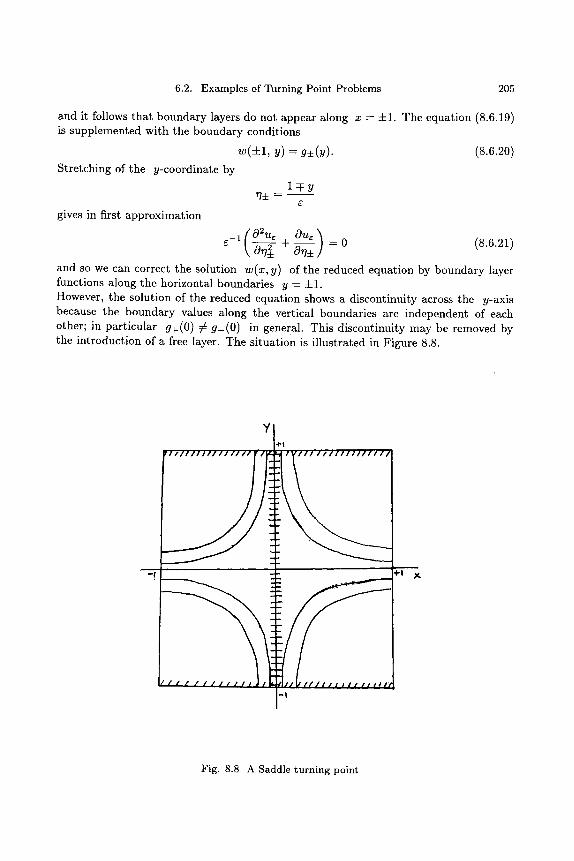
205
- t
and it follows that boundary layers do not appear along x = +1. The equation (8.6.19) is supplemented with the boundary conditions
Stretching of the y-coordinate by
gives in first approximation
w(J:l, y ) = g+(y). (8.6.20)
1 m y r/+ =
1 0r/---~--~ + ~ = 0 (8.6.21)
and so we can correct the solution w(x, y) of the reduced equation by boundary layer functions along the horizontal boundaries y = +1. However, the solution of the reduced equation shows a discontinuity across the y-axis because the boundary values along the vertical boundaries are independent of each other; in particular g+(0) # g_(0) in general. This discontinuity may be removed by the introduction of a free layer. The situation is illustrated in Figure 8.8.
u
•
6.2. Examples of Turning Point Problems
4-6 y,
Fig. 8.8 A Saddle turning point
206 Chapter 8. Perturbations of Elliptic Type
Starting with the solution w(x, y) of the reduced equation (8.6.19) with the boundary conditions (8.6.20) we obtain
w(x, y) = g+(xy), x > 0 and w(x, y) - g_(xy), x < 0 (8.6.22)
The discontinuity across the vertical axis x - 0 is removed by stretching the x coor- dinate by
x ~= v~
and by taking as a first approximation of u~(x, y)
ffJ(x, y) : g+(xy) +2 g-(xy) + 9+(xY) -2 g-(xY) erf ( ~ ) (8.6.23)
where t 2/
~rf (t) - ~ ~-~~-,-. 0
We have outside the free layer ~(x, y) ~ w(x, y) and ~ is together with its derivatives continuous across the y-axis. Further we remark that erf ( ~ ) satisfies the differential
equation (8.6.17) and a simple calculation yields
L~[~] = O(v/e) (8.6.24)
Hence zb(x, y) satisfies the differential equation (8.6.17) up to O(vf~) and the boundary conditions along the vertical boundaries up to O(e N) (N arbitrarily large). To obtain a formal approximation of u~ we have still to make a correction by bound- ary layers along the horizontal boundaries in order to satisfy also there the boundary conditions. These are constructed by solving
0~,~ 0~0~ 0,--~-~ + ~ = o, 0 < , < ~ (s.6.25)
with the boundary conditions
v~ O) = f + ( x ) - ~ ( x , • lim v~ 77) = O. ~7 ::t: - + c ~
The result reads
v~ r]+) -- v~ 1 :t:: Y) = {.f• o(x, • exp [ - 1 T Y] (8.6.26)
In order to obtain a formal approximation satisfying the differential equation and the boundary conditions up to some positive order of e we have just as in section 8.3 to add extra boundary layers ev~_ (x, L ~ ) and ev~ (x, 1+_~). These terms are only needed for
Exercises 207
the proof of the validity of the formal approximation and they may be discarded again later on. As to this proof we refer the reader to [57]. Summarizing the construction one has the result
us(x,y)=~(x,y)+v~(x, 1-Y)+v~ I + Y ) +O(x/~) (8.6.27)
where ~ is given by (8.6.23) and v~ by (8.6.26). This approximation is valid outside neighbourhoods of the points (0, +1) where the free layer and the boundary layers intersect.
Exerc i s e s
1. Determine a uniform approximation up to O(e 1/4) of the function us(x, y) that satisfies the boundary value problem
with
( 02 us 09. us ) Ous =o, x 2 + y2 = r 2 < 1,
u s = ~ ( ~ ) f o r r = l , 0<_vg_<2r, ~ ( 0 ) = ~ ( 2 r ) , ~ = a r c t a n Y . x
Ue(X , 0) -- f l ( X ) , t ts(X , ~2) -- f2 (X) , u s ( 0 , Y) = g l ( Y ) , u s ( e l , Y) --- g2(Y)
are infinitely often differentiable and continuous in the corner points.
5. Show that (8.6.16) is an approximation for the repelling node problem.
g,h�9 2<1], ~ o � 9 2 < 1.
Give first a formal approximation and consecutively its justification. See exercise 4 of Chapter 7.
4. Develop an approximation method as in Exercise 3, but now for a rectangle ; the boundary values
with
(Use the Remark 3 after section 4). 2. Consider the boundary value problem
( 02Ue O~2Ur ) -Jc -~y 2 y2 r2 - < 1
with - e c [0,
Give an approximation of ue up to O(e), uniformly valid for - 1 + 6 < x < +1 - 6 with 6 arbitrarily small positive, but independent of e.
3. Develop an approximation method for the boundary value problem
( 02u~ O2us ) e ~ + ~ +g(x,y)ue=h(x,y) forx 2 + y 2 = r 2 < 1
us=~o(vg) f o r r = l , 0 < ~ < 2 7 r , qo(0)=~0(27r), t g - a r c t a n y x

This Page Intentionally Left Blank
Chapter 9
S I N G U L A R P E R T U R B A T I O N S O F S E C O N D O R D E R H Y P E R B O L I C T Y P E .
L I N E A R T H E O R Y
1. I n t r o d u c t i o n
In this chapter we s tudy the following singular per turba t ion problem
L~[ue(x,t)] = ~L2[ue(x, t)] + Lz[ue(x, t)] = f ( x , t), t > O, -cx~ < x < +cx~, (9.1.1)
with initial values
(~U c ue(x, O) = g(x), - ~ - ( x , O) = h(x), - c ~ < x < +c~.
The differential operators L1 and L2 are given by the expressions
and
0 0 L1 = a(x, t)-O-xx" +b(x, t ) - ~ . +d(x, t).
(9.1.2)
(9.1.3)
0 2 0 2 - � 9 �9 (9.1.4) L 2 - Ot 2 OX 2
The coefficients a, b, c, the r ight-hand side f and the initial da ta g and h are for the moment arbi t rary sufficiently smooth real valued functions of x and t, respectively x. Fur thermore ~ is again a small positive parameter . This initial value problem may be considered as a per turba t ion of the initial value problem
Lz[w(x,t)] = f ( x , t ) , - c ~ < x < +c~, t > 0 (9.1.5)
with the initial condition
~(~, 0)= g(~), - ~ < �9 < + ~ . (9.1.6)
As in the preceding chapters we investigate again whether the solution of (9:1.5)-(9.1.6) is a good approximat ion of (9.1.1)-(9.1.2), and if so we investigate also the order of the approximat ion w(x, t) in terms of c.
210 Chapter 9. Perturbations of Hyperbolic Type
Problems of this kind have been studied by J.M. Blondel [12], [13], M.G. Dzavadov [28], J. Genet and G. Pupion [52], J.D. Cole [19], D.R. Smith and J.T. Palmer [128], D.R. Smith [129], M.B. Weinstein and D.R. Smith [145], [146], E.M. de Jager [77] and R. Geel [49], [47]. As physical applications we mention so-called overdamped vibration problems as occur in the propagation of electrical signals in a conducting wire of large resistance; in this case the mathematical description leads to the well- known telegraphist's equation, see [128]. Other overdamped vibration problems are for instance the motion of a vibrating string imbedded in a highly viscous medium and the propagation of radiation through a highly absorbing medium. Singular perturbation problems of hyperbolic type as treated in this and the next chapter are in a certain sense the counterparts of the perturbation problems in Chapter 6, section 6, where we discussed the averaging and the multiple scale technique for perturbed wave equations which are of the type (9.1.1)-(9.1.2) but now with E large. These singular perturbations have only after a long time a cumulative effect on the solution while the singular perturbations of this chapter have as we shall see an immediate influence on the solution.
Before we can answer the question whether the solution w(x, t) of the reduced problem (9.1.5)-(9.1.6) may be an approximation of the solution ue(x, t) of the full problem (9.1.1)-(9.1.2) we have to study first the interplay between the characteristics associated with the operator L1 and those associated with the operator L2. This will be done in the next section. In section 3 we give the formal approximation of the solution u~(x,t) and in sections 4 and 5 we show that this formal approximation is indeed a good approximation. To estimate the error term we use the energy integral method that has already been used in Chapter 7, section 1, where we discussed initial value problems for linear ordinary differential equations with a singular perturbation. We follow the theory as has been given in the references [77, 49, 47].
2. C h a r a c t e r i s t i c and S u b c h a r a c t e r i s t i c s
To get some understanding of the interplay of the characteristics of L1 and those of L2 we give in this section the discussion as presented by J.D. Cole [19]. We consider the simple perturbation problem
(0 2u~ 02u~ ) Oue b Ou~ n~[u~] = e Ot 2 Ox 2 + a--o~x + Ot = 0 ' t > 0 - c x ~ < x < + c ~ , (9.2.1)
with the initial conditions
u~(x, O) = g(x), --~-(x, O) = h(x), - c~ < x < +c~. (9.2.2)
The coefficients a and b are constants with b ~= 0 and g and h are arbitrary functions of the class 61 (-oo, +oo) and C(-cx~, +c~) respectively. The solution of the reduced initial value problem
o~ bow ~ - ~ + Ot = o, w(~, o) = g(~), (9.2.3)
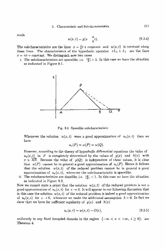
2. Characteristic and Subcharacteristics 211
reads a (9.2.4) ~ ( ~ , t) = 9(~ - gt) .
The subcharacterist ics are the lines x = ~t + constant and w(x, t) is constant along these lines. The characteristics of the hyperbolic operator eL2 + L1 are the lines x = i t + constant. We distinguish now two cases
i. The subcharacterist ics are spacelike, i.e. I~l > 1. In this case we have the si tuat ion as indicated in Figure 9.1.
P L'%
\
A B C~
Fig. 9.1 Spacelike subcharacteristic
Whenever the solution w(x, t) were a good approximat ion of ue(x, t) then we have
u~(P) ~ w(P) = w(Q).
However, according to the theory of hyperbolic differential equations the value of u~(x,t) in P is completely determined by the values of g(x) and h(x) with x E AB. Because the value of g(Q) is independent of these values, it is clear tha t w(P) cannot be in general a good approximat ion of u~(P). Hence it follows tha t the solution w(x,t) of the reduced problem cannot be in general a good approximat ion of ue(x, t), whenever the subcharacterist ic is spacelike.
a ii. The subcharacterist ics are timelike, i.e. I~l < 1. In this case we have the si tuat ion as indicated in Figure 9.2.
Now we cannot s tate a priori tha t the solution w(x, t) of the reduced problem is not a good approximat ion of uc(x, t) for e --+ 0. It will appear in our following discussion tha t in this case the solution w(x, t) of the reduced problem is indeed a good approximat ion of ue(x, t) for r --4 0, whenever we make the addit ional assumption b > 0. In fact we show tha t we have for sufficient regularity of g(x) and h(x)
u~(x , t )=w(x, t )+O(e) , (9.2.5)
uniformly in any fixed bounded domain in the region { - c ~ < x < +c~, t :> 0}; see Theorem 4.
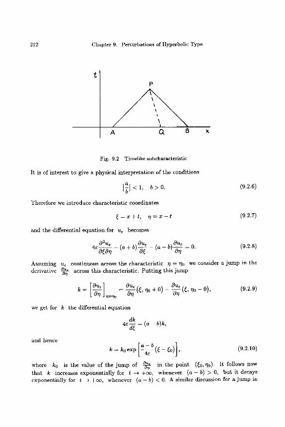
212 Chapter 9. Perturbations of Hyperbolic Type
P
A O, B
Fig. 9.2 Timelike subcharacteristic
It is of interest to give a physical interpretat ion of the conditions
a I~l < 1, b > O. (9.2.6)
Therefore we introduce characteristic coordinates
= x + t , r i = x - t (9.2.7)
and the differential equation for ue becomes
02ue Oue Oue 4r 0~0~7 - (a + b) - - ~ - (a - b) ~ = 0. (9.2.8)
Assuming u~ continuous across the characteristic 7? = rl0 we consider a jump in the derivative ~ across this characteristic. Pu t t ing this jump
on
FO_~_~ k= LOw
n=no
0. . (~. ~0 + 0) - o . . 0) o~ ~ (~' ~0- . (9.2.9)
we get for k the differential equation
dk 4 ~ : (a - b)k . a~
and hence a - b )]
k = k o e x p ~ ( , ~ - ~ o , (9.2.10)
where k0 is the value of the jump of ~ in the point (~0, rlo). It follows now on tha t k increases exponential ly for t - + +cx>, whenever (a -b ) > 0, but it decays exponential ly for t --+ +cx~, whenever (a - b) < 0. A similar discussion for a jump in
3. The Formal Approximation 213
o~ across the characterist ic ~ = ~0 gives the result t ha t the value of the j ump increases
exponential ly for t -+ +c~, whenever (a + b) < 0, but tha t it decays exponent ial ly for t -+ +c~, whenever (a + b) > 0. Therefore in the case of exponent ia l decay of jumps across characteristics we have the conditions: ( a - b ) < 0 and ( a + b ) > 0, i.e. b > lal. So we have the result tha t jumps in the derivatives across characteristics decay exponent ial ly for t --~ +cx~, whenever the subcharacterist ics are timelike with the addit ional condit ion b > 0. In the case of exponential growth of jumps across characteristics we have the conditions (a - b) > 0 and (a + b) < 0, i.e. the subcharacterist ics are spacelike.
3. The Formal Approximat ion
We consider the initial value problem (9.1.1)-(9.1.4)
Le[ue(x, t)] = cL2[ue(x, t)] + Ll[ue(x, t)] =
6 ~ -O~x2 + a(x, t) + b(x t) + d(x t)u~ - f ( x t) , ~ , ~ , , , (9.3.1)
valid for - o o < x < +c~, t > 0, while the initial conditions are given by
C~U~ ~ ( ~ , 0) = g(~), - ~ ( ~ , 0) = h(~), - ~ < ~ < + ~ . (9.3.2)
We make the following assumptions 1. All da ta are real valued with c(x, t) > O, b(x, t) > O, Vx and Vt > 0. 2. a, b, c, d and f are C~ - c ~ < x < + c ~ and t > 0 . 3. g and h are C~ for - c ~ < x < +c~. 4. There exits a number P0 # 0 such tha t
a 2 _ m . - - p2 1 b2c2 > p2, Vx and Vt > 0 (9.3.3)
5. ~ is a small positive parameter , 0 < r << 1. The assumptions 2 and 3 have been made to avoid some tedius bookkeeping; however, for less smooth functions the analysis can be carried out to a certain extent. As we have shown in the preceding section the assumpt ion 4 is necessary to obta in an approximat ion of u~ in terms of a solution of the reduced problem (~ = 0):
a(x t) Ow Ow ' -~x + b ( x ' t ) ~ + d ( x ' t ) w - f ( x ' t ) ' - c ~ < x < + c ~ , t > O (9.3.4)
with the initial condit ion
~(~ , 0 ) = g(~), - ~ < �9 < + ~ . (9.3.5)
This initial value problem is a simple linear first order problem and because of b(x, t) ~ 0 it can always be solved uniquely by the methods of characteristics; so we may assume tha t the solution w(x, t) of the reduced problem is known. This function is
214 Chapter 9. Perturbations of Hyperbolic Type
of class C ~ and it satisfies the full differential equation (9.3.1) up to O(e), uniformly in any bounded domain, and it satisfies also the first initial condition of (9.3.2), but in general not the second initial condition. Therefore we introduce a correction term v such tha t this second condition is satisfied by w + v without disturbing the first condition too much; moreover w + v should also satisfy approximately the diffferential equation at least in bounded domains in t > 0. To this end we stretch the t-coordinate by the t ransformat ion
t =er . (9.3.6)
Subst i tut ing this new variable T into L~ and retaining the main contr ibution of v(x, t) to the differential expression Le[w + v] we must require
02v Ov Ov 2 + b ( x , O ) ~ = O , 0 < r < c x ~ (9.3.7)
with the initial condition
o ~ o , (~, o ) = h(~), s t (~' o) + - ~ --cx~ < x < q-oo,
o r
Ov Ow 0 - ; (~ ,0 ) = ~ { h ( ~ ) - ( ~ , 0 ) } -07 - c ~ < x < +c~. (9.3.8)
Because (9.3.7) is of second order we need a second boundary condition for v and we take
v(x, c~) = lim v(x, ~') = 0. (9.3.9) T--~OO
This condition guarantees tha t the correction term v(x, t) has only a significant value in a small e neighbourhood of the initial line t = 0. The solution of (9.3.7)-(9.3.9) yields indeed a boundary layer function, namely
01tl) t -By(x, O) - h(x) t v(x, 7) = v(x, -~) - c. b(x, 0) exp [ - b(x, 0)~]. (9.3.10)
Pu t t ing finally
t ) + n~(x, t), u~(x, t) = w(x, t) + v(x, -~
we obtain for the remainder te rm Re the following differential equation
(9.3.11)
( 02w - c 2 ( x , t ) L~ [Re(x, t)] = - e ~ Ox 2]
+ ec2(x t) 02v Ov Ov _ d(x, t)v - a(~, t) - {b(~, t) - b(~, O) } '
0 ~ - c~(~ t) + ~c~(~, t) - ~(~, t ) - -
b(x, t) - b(x, O) Ov _ d(x t)v (9.3.12) -- t T-~T ' "
4. A Priori Estimates of Solutions of Initial Value Problems 215
From (9.3.10), the regularity of the data and from the fact that b(x,t)-b(x,O) is uniformly t bounded in any bounded domain with t > 0, we may conclude tha t
LoIRe]- O(e), (9.3.13)
uniformly in any fixed bounded domain G in the region t > 0. Moreover R~(x, t) sat- isfies the initial conditions
R~(x, O) = -v (x , O) = O(c) (9.3.14)
uniformly in any bounded interval of the x-axis, and
OR~ Ot (x, 0 ) = 0 , - c r 1 6 2 (9.3.15)
It follows that the expression w ( x , t ) + v(x, t) satisfies the initial value problem for u~(x, t) up to O(c), uniformly in any bounded domain with t > 0, and so it is a
t formal approximation of u~(x, t). To prove that w(x, t ) + v(x, -i) is indeed a good approximation of u~(x, t) we need an estimate of R~(x, t) and this est imate should be small for small values of r This estimate is obtained in the next sections with the aid of the method of energy integrals introduced by K.O. Friedrichs and H. Lewy, [44], [8].
4. A P r i o r i E s t i m a t e s of S o l u t i o n s of I n i t i a l Va lue P r o b l e m s for P a r t i a l D i f f e r e n t i a l E q u a t i o n s w i t h a S i n g u l a r P e r t u r b a t i o n of H y p e r b o l i c T y p e
We consider again our initial value problem (9.1.1)-(9..1.4)
e ~ - (z,t) 02u Ou Ou + a(x, t) Ox + b(x, t ) - ~ + d(x, t)u - f (x , t) (9.4.1)
valid for - c r < x < +cr t > O, and with the initial conditions
Ou (x, O) = h(x), - c r < x < +cr (9.4.2) u(x, O) = g(x) and -~-
As to the coefficients, the right-hand side and the initial values, we make the same regularity assumption 1-5 as in the preceeding section. The method to obtain a priori estimates of the solution u(x, t) is due to Friedrichs and Lewy [44], [8], but because of the occurrence of the small parameter c we need here a modification of this method as given in [77, 49, 47]. Multiplication of (9.4.1) with 2u gives
O (bu2 -4- 2r -4- -~-~x (au2 - 2ec2uux) = Ot
( - 2 d + bt + ax)u 2 + 2ca 2 - 2ec2u 2 - 2e(c2)~uu~ + 2fu,
where we have omitted the arguments of the functions involved. Multiplication of (9.4.1) with 2but and 2au~ gives respectively
0 0 (~b~ + ~ b c ~ ) + ( -2~bc~u~) = 0-~
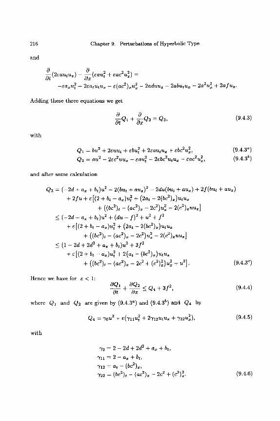
216 Chapter 9. Perturbations of Hyperbolic Type
and
0 0 (~au 2 -4- ~ac2u 2) - Ot (2eau t u~ ) - -~x
2 _ 2aduu~ - 2 a b u t u z 2a2u 2 + 2 a l u m . - e a ~ u 2 + 2 e a t u t u x - e ( a c 2 ) ~ u ~
Adding these three equations we get
o o oq-~Q1 + ~xQ2 = Q3, (9.4.3)
with
Q1 - bu 2 + 2 e u u t + ebu2t + 2 e a u t u z + ebc2u2z, 2 Q2 = au2 - 2ec2uux - e a u 2 - 2ebc2u tuz - eac2ux ,
(9.4.3 a)
(9.4.3 b)
and after some calculation
Q3 = ( - 2 d + a~ + b t )u 2 - 2(but + aux ) 2 - 2du(bu t + au~) + 2 f ( b u t + a u z )
+ 2 f u + E[(2 + bt - a ~ ) u 2 + (2at - 2 (bc2)~)u tu~
~ 2 ( c ~ ) ~ ] + ( ( b c 2 ) t - (ac2)x - 2c2)u~ -
< ( - 2 d + a ~ + b t ) u 2 + ( d u - f ) 2 + u 2 + f 2
+ c[(2 + bt - a~ )u 2 + (2at - 2 ( b c 2 ) ~ ) u t u x
+ ( (bc~)~- ( a ~ ) ~ - 2 ~ ) = ~ - 2 ( ~ ) ~ = u ~ ]
< (1 - 2d + 2d 2 + a~ + bt)u 2 + 3f 2
+ c[(2 + bt - a~ )u 2 + 2 (a t - (bc2)~)u tu~
2 + ( ( b c 2 ) t - (ac2)x - 2c 2 + (c2)2)ux + u2]. (9.4.3 ~)
Hence we have for E < 1" OQ1 OQ2 0--~ + - ~ x < Q4 + 3f 2
where Q1 and Q2 are given by (9.4.3 a) and (9.4.3 b) and Q4 by
(9.4.4)
Q4 -- ~0 ~2 -~- E(")'ll u2 -~- 2~[12~tUx -Jr-~22'tt2), (9.4.5)
with
3'0 = 2 - 2d + 2d 2 A- ax + bt,
711 = 2 - az + bt ,
") '12 = at -- (bc2)z,
7 ~ = (b~ ~)~ - ( a ~ ) ~ - 2 ~ + (c ~) x " (9.4.6)
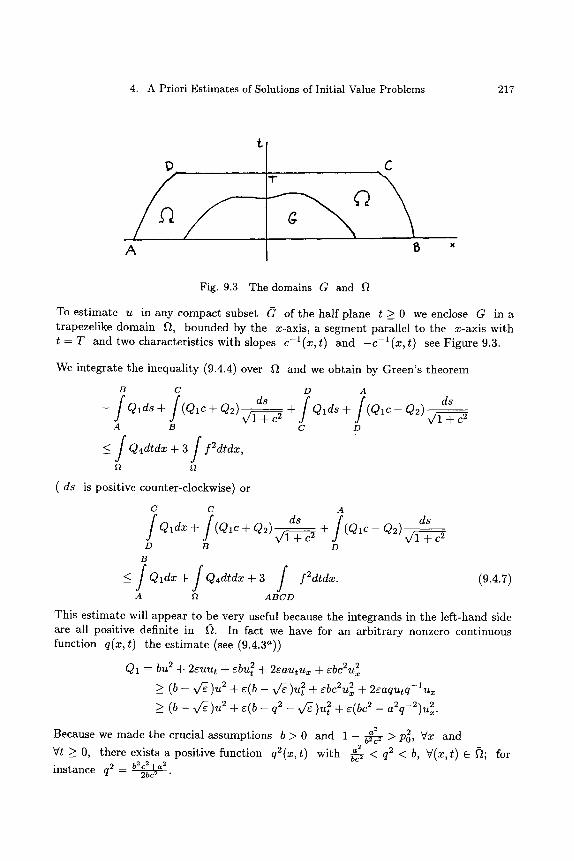
4. A Priori Estimates of Solutions of Initial Value Problems 217
C
A B X
Fig. 9.3 The domains G and
To es t imate u in any compact subset (~ of the half plane t > 0 we enclose G in a trapezelike domain Ft, bounded by the x-axis, a segment parallel to the x-axis with t = T and two characteristics with slopes c-l(x,t) and -c- l (x , t ) see Figure 9.3.
We integrate the inequali ty (9.4.4) over ~t and we obta in by Green 's theorem
B C
- Qlds+ (Qlc+Q2) x / l+c 2 A B
<_ / Q4dtdx + 3 / f2dtdx,
( ds is positive counter-clockwise) or
D A
C D
C C A
ds VII ~-c 2
/ / ds / Q~dx + (Q~c + Q2) x/l + c 2 + (Q~c- Q2) v/1§ c2
D B D
B
<_ / Qldx + / Q4dtdx + 3 / f2dtdx. (9.4.7)
A ~ A B C D
This es t imate will appear to be very useful because the integrands in the left-hand side are all positive definite in ~t. In fact we have for an arb i t rary nonzero continuous function q(x, t) the es t imate (see (9.4.3a))
Q1 = bu 2 + 2guut ~- sbu2t + 2--cautux -[- -cbc2u 2 _> ( b - x/~)u 2 + ~(b- V~)u2t + cbc2u 2 + 2~aqutq-Xux _ 2 > ( b - v~ )~ : + ~ ( b - q~ - v ~ ) ~ + ~(b~ ~ - a~q-~)~.
a 2
Because we made the crucial assumptions b > 0 and 1 - ~ > p0 2, Vx and _ , a ~ q 2 Vt > 0 there exists a positive function q2(x, t) with b-fi < < b, V(x, t) C ~; for
i n s t a n c e q2 _ b 2c 2 + a 2 - - 2bc 2 �9
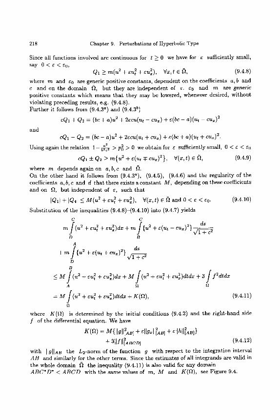
218 Chapter 9. Perturbations of Hyperbolic Type
Since all functions involved are continuous for t > 0 we have for 6 sufficiently small, say 0 < 6 < 6 0 ,
Q1 >_ m(u 2 + 6u 2 + 6u2), Vx, t �9 ~t, (9.4.8)
where m and 60 are generic positive constants, dependent on the coefficients a,b and c and on the domain l~, but they are independent of 6. 60 and m are generic positive constants which means tha t they may be lowered, whenever desired, without violating preceding results, e.g. (9.4.8). Further it follows from (9.4.3 a) and (9.4.35)
cQ1 + Q2 = (bc + a)u 2 + 26cu(ut - cux) + 6 (bc - a)(ut - cux) 2
and cQ1 - Q2 = ( b c - a)u 2 + 26cu(ut + cu,) + 6(bc + a)(ut + cu,) 2.
Using again the relation 1 - g~-/-~2 > p2 > 0 we obtain for 6 sufficiently small, 0 < 6 < 60
cQ1 + Q2 >_ m { u 2 + 6(ut T cu,)2}, V(x, t) �9 ~t, (9.4.9)
where m depends again on a,b,c and Ft. On the other hand it follows from (9.4.3~), (9.4.5), (9.4.6) and the regularity of the coefficients a, b, c and d that there exists a constant M, depending on these coefficients and on ~t, but independent of 6, such that
IQ~I + IQ41 5 M ( u 2 + 6u 2 + 6u2), V(x, t) �9 l~ and 0 < 6 < 60. (9.4.10)
Substi tution of the inequalities (9.4.8)-(9.4.10)into (9.4.7)yields
C C / / ds m (u 2 + eu2t + eu~)dx + m {u 2 + e(ut - cux) 2} x/1 + c - - - - - ~
D B A
+ m / { u 2 + e(ut + cux) 2} d s ~/1 + c 2
D B
A ~2
- M / ( U 2 + eU 2 + r + K(ft) ,
12
(9.4.11)
where K(ft) is determined by the initial conditions (9.4.2) and the right-hand side S of the differential equation. We have
K(Q) = M{[lg[I~AB] + r + ellhll~AB]}
+ 3I[fll~ABCD ] (9.4.12)
with Jig]lAB the L2-norm of the function g with respect to the integration interval A B and similarly for the other terms. Since the estimates of all integrands are valid in the whole domain ~ the inequality (9.4.11) is also valid for any domain ABC*D* < A B C D with the same values of m, M and K(ft) , see Figure 9.4.
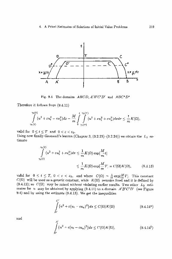
4. A Priori Estimates of Solutions of Initial Value Problems 219
/ ,, A A'
•
T .. C
B" B ~'
Fig. 9.4 The domains ABCD, AIBICID! and ABC*D*
Therefore it follows from (9.4.11)
-~ (t) t "y~ (,-)
f (u2 +eu2t +eu2)dx-M-M-m f f (u2 +eu2t nt-eu2x)dxdT<-1K(ft)'m "n (t) o "n (~)
valid for 0 _ < t _ < T and 0 < e < e 0 . Using now finally Gronwall's lemma (Chapter 3, (3.2.23)-(3.2.24)) we obtain the L2 es- t imate
-r~ (t)
/ (u2+eu2+eu2)dx<-1K(ft) e x p [ M t ] m
,~(t)
< 1K(ft)m exp[MT] = C(ft)K(ft), (9.4.13)
1 exp[MT]. This constant valid for 0 < t _< T, 0 < e < e0, and where C(ft) = C(ft) will be used as a generic constant, while K(ft) remains fixed and it is defined by (9.4.12); so C(ft) may be raised without violating earlier results. Two other L2 esti- mates for u may be obtained by applying (9.4.11) to a domain A'B'C'D' (see Figure 9.4) and by using the estimate (9.4.13). We get the inequalities
C !
{u + e(ut - cux)2}ds <__ C(ft)K(gt) B '
(9.4.14 a)
and A !
{u + e(ut + cu~)2}ds < C(fI)K(~), D '
(9.4.14 b)
220 Chapter 9. Perturbations of Hyperbolic Type
valid for all characteristic segments B'C' and D'A' inside ~ and for all c sufficiently small, 0 < e < ~0. Now that we have derived three estimates in L2 norm for a combination of u and its first derivatives it is not difficult to get a pointwise estimate for the function u(x, t) , uniformly valid for ~ sufficiently small in ft. Wi th the aid of the Schwarz inequality we have the following estimates in fl, (see Figure 9.4),
lu2(x,t) - u2(~(t), t ) l - - 2 ] u(~,t)u~(~,t)d~ < 2 ] lu(~,t)i" iu~(~,t)id~ ~l(t) ~(t)
} < 2 u2(~, t)d~ u,(~, t)d~ . ~(t) ~1(t)
Using once again (9.4.13) we get
lu2(x, t ) - u2(Ti(t), t I __ e-�89
o r
u2(71 (t), t) < u2(x, t) + C(fl)K(~2)e-�89
After integrating this result with respect to x between the limits 71(t) and 72(t) we have
~2(t)
01u2(')'l(t), t) <__ f uZ(x,t)dx + 02C(f~)K(f~)e-�89 71(0
with
= max / ' ' ' ' x " r ' / 2 t t j - 7 1 t t j j = n B . 0 1 - - min ( 7 2 ( t ) - 71(t)) = C D and 82 0<t<T 0 < t < T
Once again with (9.4.13) we obtain
01u2(71(t), t) < C(f~)g(f~)(1 + 02e-�89
because also u2(x,t) <_ u2(71(t), t) + C(a)g(~)c-�89
we get finally u2(x,t) < C ( a ) g ( ~ ) { 0 1 1 + (02011+ 1)E-�89 },
or after absorption of (020~ -1 + 1) in C(D)
u(x, t) <_ v/C(f~)g(f~) e-�88 (9.4.15)
uniformly in ABCD for ~ sufficiently small, say 0 < e < e0. We can derive also pointwise estimates for the derivatives ux(x, t) and ut(x, t); we proceed as follows, see Figure 9.5.
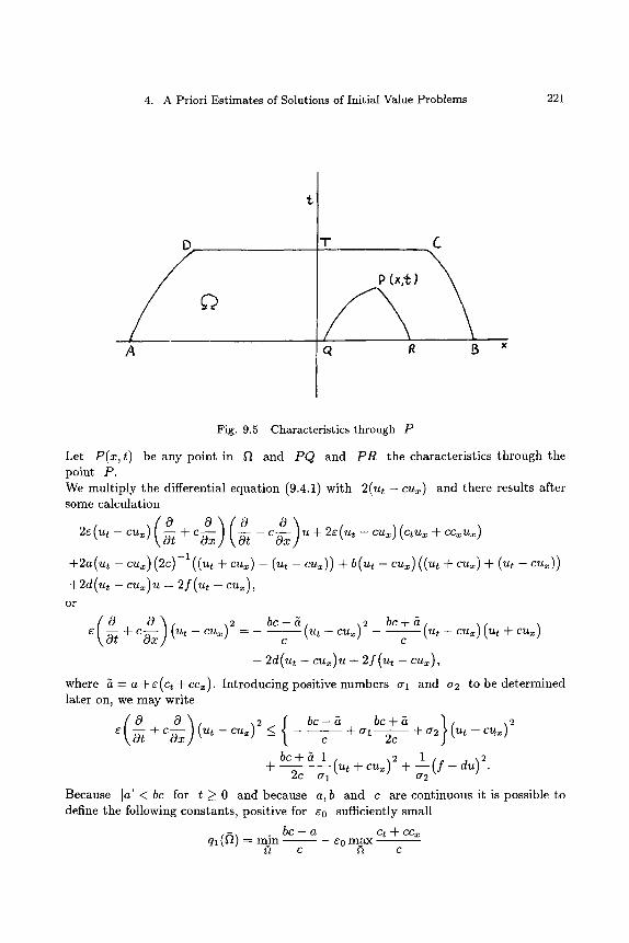
4. A Priori Estimates of Solutions of Initial Value Problems 221
�9
A
T d
P (x,'~)
~ R 5
Fig. 9.5 Characteristics through P
Let P ( x , t ) be any point in ~ and P Q and P R the characteristics through the point P. We multiply the differential equation (9.4.1) with 2(ut - c u ~ ) and there results after some calculation
2e ( ut - cu~ ) --~ + c-~-~x --~ - c-~-~x u + 2r ( ut - cu~ ) ( ct u~ + cc~ ux )
+ 2 a ( u t - cu~) (2c) -1 ((ut + cu~) - (ut - cu~)) + b(ut - cu~) ((ut + cu~) + (ut - cu~))
+ 2 d ( u t - c u x ) u = 2 f (ut - cu~), o r
0 c o ) 2 -~+ ~ (u~-~u~) = b ~ - a (~ ,_ ~ ) ~ . b~+ a ( ~ , _ c ~ ) ( ~ + ~ ) C C
where 5 = a + e ( c t + cox). Introducing positive numbers 0"1 and 0"2 to be determined later on, we may write
~ + ~ (u, - cu~) < ~ ~ + ~ (~, - c ~ ) ~ - c 2 c '
1 b c + 5 1 (ut +cux)2 + - - ( f - d u ) 2 -4 2C 0.1 0"2 "
Because la[ < bc for t > 0 and because a,b and c are continuous it is possible to define the following constants, positive for e0 sufficiently small
(~) min bc - a ct + cc~ ql ~ -- eo m a x
c ~2 c
222 Chapter 9. Perturbations of Hyperbolic Type
and bc + a ct + ccx
q2(~) = max ~ + s0 max 12 c ~ c
These constants depend only on a ,b ,c and ~, but they are independent of s. Substituting these constants in the last inequality there results
s -~ + C-~x (ut - cu~) 2 _ { - ql (~) + alq2(~) + a2 }(ut - cu~) 2
1 d_ q2(~) a 11 (ut d- CUx) 2 -4- --a2 ( f -- du)2' uniformly in ~ for 0 < s < So.
1 Choosing a l q 2 ( ~ ) = [ q l ( ~ ) and a2 = l q l ( ~ ) we obtain the estimate
0 O) 2 1 1 ~ + c ~ (=, - c=~) < q , . ( ~ ) - ( = , + c ~ ) ~ + - ( f - ~=)~
6r 1 (7 2
_ 2q~ (~t) 4 - q~(5) (=, + c=~): + (I - d=) ~
ql(~)
uniformly in ~ for 0 < s < s 0 . Consecutively we integrate this inequality along the characteristic P Q and we get with the aid of (9.4.145 )
2q2(~) 1 s(ut - cu~)2(P) < s(ut - cu~)2(Q) + - C(f~)K(f~)
ql (12) s Q
+ (f2 + d2u2)ds. ql(~)
P
Using again the regularity of the data of the initial value problem and the estimate (9.4.15) we obtain finally in Ft the uniform estimate
lu,- c~) < v /C(~ t )K( f~ ) s -1, V(x, t) e ~, 0 < s < s0,
where the constants ql(~) and q2(~) have been absorbed in the generic constant c(a). Quite similarly we have also
lu~ + c~=l < v/C(12)K(12)e -1, V(x,t) e ~, 0 < e < e0.
Hence we have finally obtained besides the pointwise estimate (9.4.15) for the solution u(x, t) of the initial value problem (9.4.1)-(9.4.2) also the pointwise estimates for the derivatives ux(x , t) and at(x, t):
ux(x , t) < v /C(f~)K(f~) S -1 Ut(X , t) < v/C(f~)K(f~) s -1, (9.4.16)
5. The Estimate of the Remainder Term and Final Results 223
uniformly valid in ~ for r sufficiently small; C(~t) depends on the coefficients a, b, c, d and the domain ~t, while g(~t) is defined by (9,4,12).
Summarizing we have proved the next theorem
THEOREM 1 The solution of the initial value problem
02u _ c 2 } b-~ (x, t) 02u Ou Ou + a(x, t) -~x + b(x, t) -ff[ + d(x, t)u - f (x, t)
- c x ~ < x < + o o , t > O , O < e ~ l ,
o~ (~, 0 ) = h(~), - o ~ < �9 < +o0 with u(x, O) = g(x),
has under the regularity assumptions 1-5 of section 3 for e sufficiently small the following pointwise estimates, uniformly valid in any compact domain G with t >_ O,
u(x,t) < e-�88 v/C(f~)K(f~)
ux(x, t) < ~-1 v/C(~)K(f~)
ut(x,t) < e-1 v/C(~)K(~t).
(9.4.17)
(9.4.18)
(9.4.19)
The constants C(f~).and K(~) depend on the coefficients a,b,c,d and the domain f~, while K(~2) depends also on the right-hand side f and on the initial data g and h; the latter is given by the relation (9.4.12).
5. T h e E s t i m a t e of t h e R e m a i n d e r T e r m a n d F ina l R e s u l t s
We return to our formal approximation of the initial value problem (9.1.1)-(9.1.4). The result reads
ue(x,t) = w(x,t) + v(x, t ) + Re(x,t) , (9.5.1) c
where w(x, t) is the solution of the reduced problem
a(~, t) O~ Ow -~x + b(x, t) - ~ + d(x, t)w = f (x, t)
~(~ , o ) = g(~),
--cx3 < x < cx3, t > 0,
t and v(x, -i) is the boundary layer correction given by (9.3.10). The remainder term Re(x, t) satisfies according to the equations (9.3.12)-(9.3.15) the initial value problem
( 0 2 R e _ c2(x, t) O2Re ) ORe Ot 2 Ox 2 + a(x, t) -~x + b(x, t) + d(x, t)R~ = O(e), (9.5.2)
uniformly in any compact domain in t > 0, with the initial conditions
R~(~, 0) = - ~ ( ~ , 0) = - ~ Ot
b(~,o) = o(~)
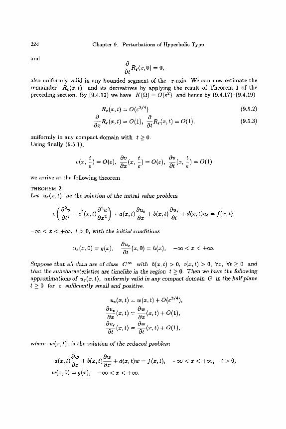
224 Chapter 9. Perturbations of Hyperbolic Type
and
0--R~(~, 0)=0, Ot
also uniformly valid in any bounded segment of the x-axis. We can now est imate the remainder Re(x , t ) and its derivatives by applying the result of Theorem 1 of the preceding section. By (9.4.12) we have g (g t ) = O(c 2) and hence by (9.4.17)-(9.4.19)
Re(x, t) = O(e 3/4) (9.5.2)
0 0 -~xxRe(x,t) = O(1), -~Re(x , t ) = O(1), (9.5.3)
uniformly in any compact domain with t > 0. Using finally (9.5.1),
Ov t =0(1) ,(x, ;t) = 0(~), ~(~,;a, t) = 0(~), -b-;(~, ;)
we arrive at the following theorem
THEOREM 2 Let ue(x, t) be the solution of the initial value problem
\ c9t2 -- c9x2 ] + a(x, t) + b(x, t) + d(x, t)ue - f ( x , t) -g7
- c o < x < +oc, t > O, with the initial conditions
OUe (x,O) = h(x), - c r 1 6 2 ~ ( ~ , O) = g(~), -g-f
Suppose that all data are of class C ~ with b(x, t) > O, c(x, t) > O, Vx, Vt > 0 and that the subcharacteristics are timelike in the region t > O. Then we have the following approximations of ue(x, t), uniformly valid in any compact domain G in the half plane t > 0 for r sufficiently small and positive.
u~(x, t) = w(x, t) + 0(~3/4), Ou~ (x, t) = Ow cox -~x (x' t) + O(1)'
OUe (x t) = cgw Ot ' --~-~(x,t) + 0(1) ,
where w(x, t) is the solution of the reduced problem
a(x, t) Ow O~ -~x + b(x, t) ~ + d(x, t)w = f ( x , t),
w ( x , O ) = g ( x ) , --cx3 < x < +cx3.
- o o < x < A-co, t > O ,
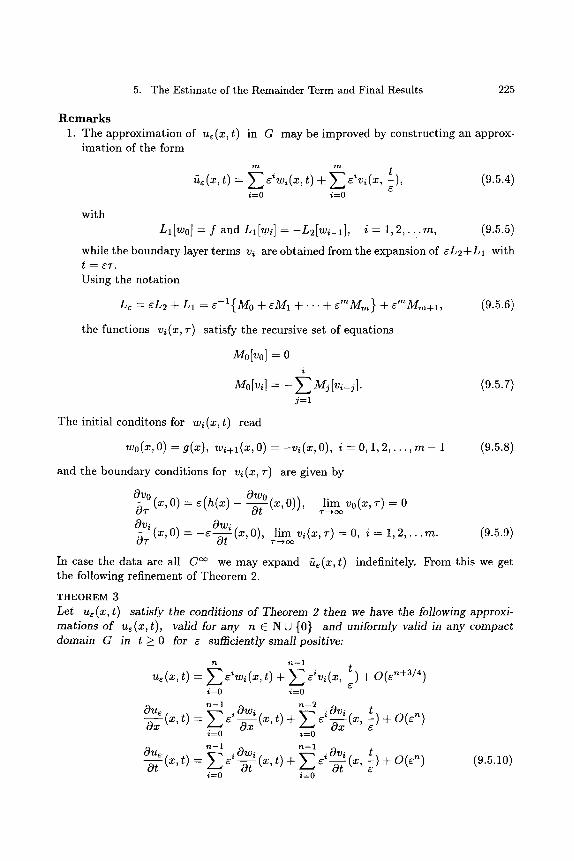
5. The Estimate of the Remainder Term and Final Results 225
Remarks 1. The approximation of ue(x, t) in G may be improved by constructing an approx-
imation of the form
m m 4 -
(,~(x, t) - E eiw'(x' t) + E eiv,(x, ~), (9.5.4) i--0 i--0
with Ll[w0] = f and Ll[W.i] = -L2[wi-1], i = 1, 2 , . . . m , (9.5.5)
while the boundary layer terms vi are obtained from the expansion of r with t - - ~ T . Using the notation
Le - gL2 + L1 - e-1 {M0 + gM1 + . . . + gmMm} + gmMm+l, (9.5.6)
the functions vi(x, T) satisfy the recursive set of equations
M0[v0] = 0 i
Mo[vi] - - E Mj[vi_j]. (9.5.7) j--1
The initial conditons for wi(x, t) read
Wo(X , O) -- g (x ) , Wi+ 1 (X, O) -- --Vi(X, 0) , i --- O, 1, 2 , . . . , m - 1 (9.5.8)
and the boundary conditions for vi(x, T) are given by
Ovo Owo OT (x, O) -- e(h(x) - ~ ( x , 0)), l i ra Vo(X, T) = 0
OVioT (X, O) = --C--~OWi (X, 0), ~-~lim vi(x, T) = 0, i = 1, 2 , . . . m . (9.5.9)
In case the data are all C ~ we may expand Cte(x,t) indefinitely. From this we get the following refinement of Theorem 2.
T H E O R E M 3
Let u~(x, t) satisfy the conditions of Theorem 2 then we have the following approxi- mations of u~(x, t), valid for any n C N t3 {0} and uniformly valid in any compact domain G in t >_ 0 for e sufficiently small positive:
n--1 Ue(X , t) : c iw i (x , t) + E ~iv i (x ' t ) + 0 ( ~ n + 3 / 4 )
E i=0 i--0
0 U e n - 1 n--2 t) + - ) +
i=0 i=0
Ou,ot (x, t) = E r - ~ ( x , + r -~Ovi (x, ~t) + 0 (~,~) (9.5.10) i=0 i=0
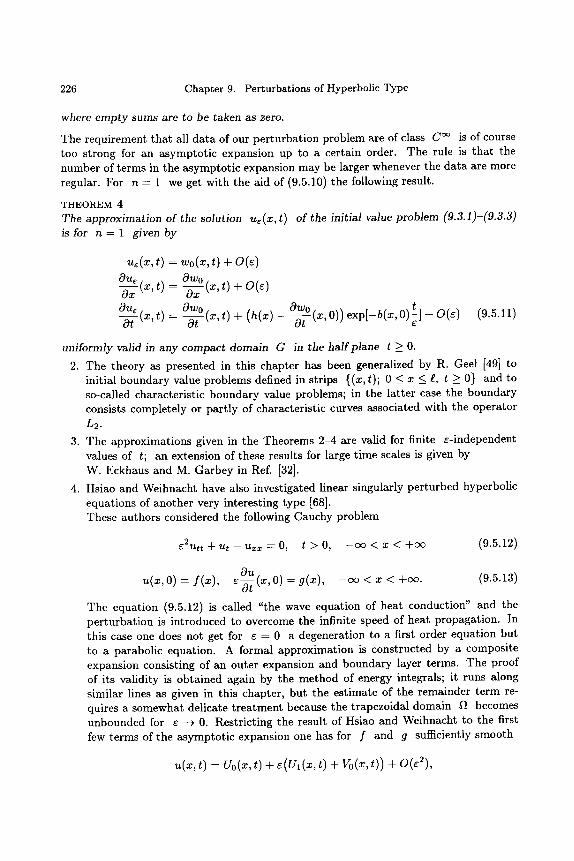
226 Chapter 9. Perturbations of Hyperbolic Type
where empty sums are to be taken as zero.
The requirement that all data of our per turbat ion problem are of class C ~ is of course too strong for an asymptotic expansion up to a certain order. The rule is that the number of terms in the asymptotic expansion may be larger whenever the data are more regular. For n = 1 we get with the aid of (9.5.10) the following result.
THEOREM 4 The approximation of the solution u~(x, t) of the initial value problem (9.3.1)-(9.3.3) is for n = 1 given by
~,(~, t) = ~0(~, t) + o(~)
Ou~ (~, t) = O~o (~ t) + o(~) oz ~ ' Ou~ Owo Owo t ot (~' t) = - -~ (~, t) + (h(~) - --07- (~, o)) ~xp[-b(~, o) ~] + o(~) (9.5.11)
uniformly valid in any compact domain G in the half plane t >_ O.
2. The theory as presented in this chapter has been generalized by R. Geel [49] to initial boundary value problems defined in strips {(x, t); 0 < x _< s t >__ 0} and to so-called characteristic boundary value problems; in the latter case the boundary consists completely or part ly of characteristic curves associated with the operator
L2.
3. The approximations given in the Theorems 2-4 are valid for finite e-independent values of t; an extension of these results for large time scales is given b y W. Eckhaus and M. Garbey in Ref. [32].
4. Hsiao and Weihnacht have also investigated linear singularly perturbed hyperbolic equations of another very interesting type [68]. These authors considered the following Cauchy problem
e 2 u t t + u t - u * * : O , t > O , - c ~ < x < + c ~ (9.5.12)
OU(x, O) = g(x), - c ~ < x < +oo. (9.5.13) u(~, o) = y(~), ~
The equation (9.5.12) is called "the wave equation of heat conduction" and the perturbat ion is introduced to overcome the infinite speed of heat propagation. In this case one does not get for r = 0 a degeneration to a first order equation but to a parabolic equation. A formal approximation is constructed by a composite expansion consisting of an outer expansion and boundary layer terms. The proof of its validity is obtained again by the method of energy integrals; it runs along similar lines as given in this chapter, but the estimate of the remainder term re- quires a somewhat delicate t reatment because the trapezoidal domain 12 becomes unbounded for 6 --4 0. Restricting the result of Hsiao and Weihnacht to the first few terms of the asymptotic expansion one has for f and g sufficiently smooth
u(~, t) = Uo(~, t) + ~(u, (~, t) + Vo(., t)) + o ( ~ ) ,
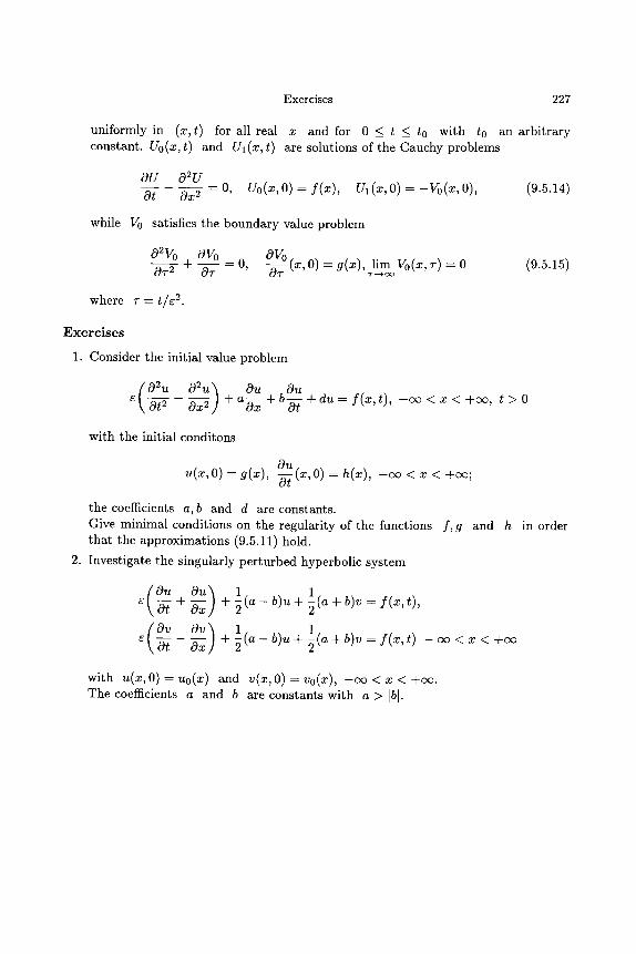
Exercises 227
uniformly in (x,t) for all real x and for 0 _< t _< to with to an arbitrary constant. Uo(x, t) and [/1 (x, t) are solutions of the Cauchy problems
OU 02U 0t 0X 2
= O, Uo(x, O) = f ( x ) , U1 (x, O) = - V o ( x , 0), (9.5.14)
while V0 satisfies the boundary value problem
O2Vo Oyo Oyo OT---- W + ~ = O, --ff~T (X, O) = g(x) , l i r n V0(x, T) = 0 (9.5.15)
where T - t / r 2.
Exercises
1. Consider the initial value problem
02u
Ot 2 02u ) Ou Ou O x 2 + a ~x q- b --~ + d u - f ( x , t ) , - cx) < x < q- cx~ , t > 0
with the initial conditons
()U ~(~, 0) = g (~ ) , ~ (~, 0) = h(~) , - ~ < ~ < +oo;
the coefficients a,b and d are constants. Give minimal conditions on the regularity of the functions f, g and h in order that the approximations (9.5.11) hold.
2. Investigate the singularly perturbed hyperbolic system
( ) 1 - ~ q- Ou q- -21 (a - b)u q- -~ (a q- b)v -- f (x, t),
( ) 1 e Ovot oxOV + 2 1 ( a - b ) u + - ~ ( a + b ) v = f ( x ' t ) - c x D < x < + o o
with u ( x , O ) = uo(x) and v ( x , O ) = v o ( x ) , - c o < x < +c~. The coefficients a and b are constants with a > [b[.

This Page Intentionally Left Blank
Chapter 10
S I N G U L A R P E R T U R B A T I O N S IN N O N L I N E A R I N I T I A L V A L U E P R O B L E M S
OF S E C O N D O R D E R
1. I n t r o d u c t i o n
In this chapter and the next one we will discuss singular perturbations in nonlinear problems. Due to the large variety of possible nonlinear differential equations and the analytical difficulties concerning the integrability and the uniqueness of solutions we are forced to restrict our exposition to some relatively simple types for which we investigate whether the linear theory as treated in the preceding chapters may be generalized. This means that we discuss in this and the next chapter only second order scalar problems; we start with initial value problems since these are more easily to handle than boundary value problems.
In the same way as in the preceding Chapters 7 and 9 we construct a formal approx- imation of the solution and in order to show that this approximation is indeed a good one we should give an a priori estimate of the remainder term that satisfies a singularly perturbed nonlinear initial value problem with the right-hand side of the differential equation and the initial values being small in some order of ~.
Functional analysis provides very useful means for getting a priori estimates of solutions of nonlinear differential equations; so several authors, e.g. Hoppenstead [66], [67], Krein [88], van Harten [64], [62], Besjes [9], Geel [49], [48], Geel and de Jager [46, 75], Genet and Madaune [51]-[102], Hsiao, Weihnacht and Esham [69, 34, 36, 39, 40, 35, 38] applied principles from functional analysis to the study of singular perturbation problems. In section 2 we derive a contraction theorem in a Banach space, due to a.o. van Harten [64], [62], which is very useful to obtain the required estimate of the remainder term. This theorem will also be used in the next chapter where we discuss boundary value problems. Section 10.3 is devoted to initial value problems of the type
d2u du du r 2 + a(X, u) ~ + b(x, u) = O, u(O) -- a, ~x (O) = fl, (10.1.1)
and section 10.4 to the more general nonlinear initial value problem
d2u du du e-~x2 = f ( u , ~xx) , u(O) = a, ~x(O) = j3 (10.1.2)
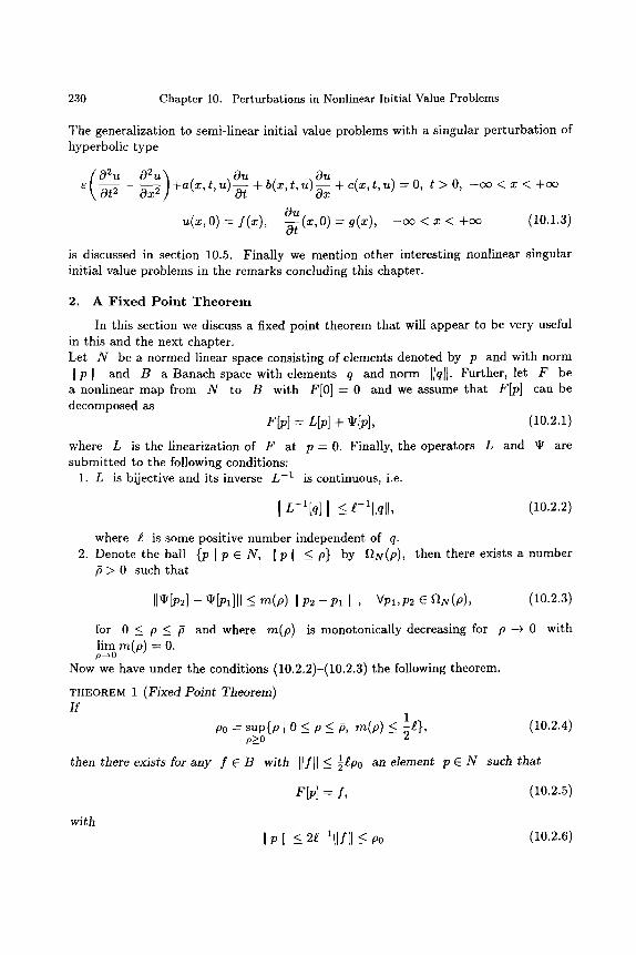
230 Chapter 10. Perturbations in Nonlinear Initial Value Problems
The generalization to semi-linear initial value problems with a singular perturbat ion of hyperbolic type
( 02u 02U ) +a(x, t, u) OU Ou ot~ o ~ Y i + b(~, t, u ) ~ + c(~, t, ~,) : o, t > o, - ~ < ~ < +o0
OU(x, O) = g(x), - c o < x < +co (10.1.3) u(x, O) -= f(x), -~
is discussed in section 10.5. Finally we mention other interesting nonlinear singular initial value problems in the remarks concluding this chapter.
2. A F i x e d P o i n t T h e o r e m
In this section we discuss a fixed point theorem that will appear to be very useful in this and the next chapter. Let N be a normed linear space consisting of elements denoted by p and with norm I p l and B a Banach space with elements q and norm [[q[[. Further, let F be
a nonlinear map from N to B with F[0] = 0 and we assume that F[p] can be decomposed as
F[p] = Lip] + ~[p], (10.2.1)
where L is the linearization of F at p - 0. Finally, the operators L and �9 are submitted to the following conditions:
1. L is bijective and its inverse L -1 is continuous, i.e.
[ L-l[q] [ <-- ~-~llqll, (10.2.2)
where ~ is some positive number independent of q. 2. Denote the ball {p I P E N, [ p [ <_ p} by ftN(p), then there exists a number
fi > 0 such that
II~[p2]- ~[p~]ll _< re(p) I p~ - p l I , vpl,p2 e aN(p), (10.2.3)
for 0 _~ p _< p and where re(p) is monotonically decreasing for p -+ 0 with lim re(p) = O. p--~0
Now we have under the conditions (10.2.2)-(10.2.3) the following theorem.
THEOREM 1 (Fixed Point Theorem) If
1
p o = s u p { p [ O ~ P ~ f i , rn(p) ~ ~s (10.2.4) p_>o
then there exists for any f E B with [[fl]-< �89 an element p E N such that
F[p] = f, (10.2.5)
with [P [ <- 2e-l[[f[[ ~ P0 (10.2.6)
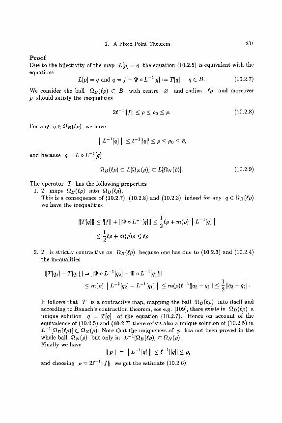
2. A Fixed Point Theorem 231
P r o o f Due to the bijectivity of the map Lip] = q the equation (10.2.5) is equivalent with the equations
L [ p ] = q a n d q = f - q 2 o L - l [ q ] : = T [ q ] , q e B . (10.2.7)
We consider the ball ~B(~.p) C B with centre ~ and radius ip and moreover p should satisfy the inequalities
2g-lllfll < p ~ po < ~. (10.2.8)
For any q G ~B(~.p) we have
I L-l[q] ] -< ~-~llqll-< p -< p0 _< Z,
and because q = L o L-I[q]
~2S(ip) C L[~2N(p)] C L[~2N(~)]. (10.2.9)
The operator T has the following properties 1. T maps F~s(ip) into ~B(t.p).
This is a consequence of (10.2.7), (10.2.8) and (10.2.3); indeed for any q e F~B(~.p) we have the inequalities
1 [[T[q][[ ~< [Ifll + I1~ o L-l[q][[ <~ -~M-4- re(p) I L-X[q] [
1 < -~.p + m(p)p < ~p
2
2. T is strictly contractive on F~B(ip) because one has due to (10.2.3) and (10.2.4) the inequalities
lIT[q2] - T[ql]I] = II~ o L - I [ q 2 ] - ~ o L-I[ql]II 1
< re(p) I n -~ [q2] - n-~[q~] I < m(p)e-~l lq2- qlll < ~ l lq2- q~[I.
It follows that T is a contractive map, mapping the ball ~B(~p) into itself and according to Banach's contraction theorem, see e.g. [109], there exists in ~B(iP) a unique solution q = T[q] of the equation (10.2.7). Hence on account of the equivalence of (10.2.5) and (10.2.7) there exists also a unique solution of (10.2.5) in L-I[~B(~.p)] C ~N(P). Note that the uniqueness of p has not been proved in the whole ball fiN(P) but only in L-l[g~B(t.p)] C F~N(p). Finally we have
I p l = [ L-~[q] [ < t-lllqll < P,
and choosing p = 2g-xllfll we get the estimate (10.2.6).
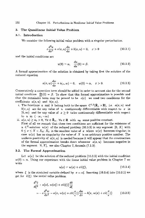
232 Chapter 10. Perturbations in Nonlinear Initial Value Problems
3. T h e Quasi l inear Initial Value P r o b l e m
3.1. I n t r o d u c t i o n
We consider the following initial value problem with a singular perturbation.
d2u du r + o(x u) + b(x u) = 0, x > 0 (10.3.1)
' -~x '
and the initial conditions are
du u(0) = c~, ~xx(0) = ~. (10.3.2)
A formal approximation of the solution is obtained by taking first the solution of the reduced equation
a(x, w) dw -~x + b(x, w) = 0, w(0) = (~, x > 0. (10.3.3)
Consecutively a correction term should be added in order to account also for the second initial condition d= ~ ( 0 ) = ~. To show that this formal approximation is possible and that the remainder term may be proved to be o(e) we need two conditions for the coefficients a(x, u) and b(x, u).
i. The functions a and b belong both to the space C1'2(1~,+ x R), i.e. a(x,u) and b(x, u) are for any value of u continuously differentiable with respect to x in [0, cx3) and for any value of x > 0 twice continuously differentiable with respect to u in (-cr
ii. a(x, u) > a0 > 0, Vx E I~,+, Vu E R with a0 some positive constant. First of all we remark that these two conditions are sufficient for the existence of a C2-solution w(x) of the reduced problem (10.3.3) in any segment [0, X] with 0 < x < X < X0; X0 is the smallest value of x where w(x) becomes singular; in case w(x) has no singularity the value of X is an arbitrary positive number. The uniform positivity of a(x, u) is needed because it will appear that the construction of the formal approximation breaks down whenever a(x, u) becomes negative in the segment [0, X], see also Chapter 7, formula (7.1.3).
3.2. T h e Formal A p p r o x i m a t i o n
Let w(x) be the solution of the reduced problem (10.3.3) with the initial condition w(0) = c~. Using our experience with the linear initial value problem in Chapter 7 we write
u(x) = w(x) + ~9(~), (10.3.4)
where ~ is the stretched variable defined by x = e~. Inserting (10.3.4) into (10.3.1) we get for ~(~) the initial value problem
d2v d~ d~ 2 + a ( ~ , w(6~) + 69(~)) d~
d2w dw = -- e~x 2 - a(x, w(x) + eg(x))-~x -- b(x, w(x) + 69(x)) (10.3.5)
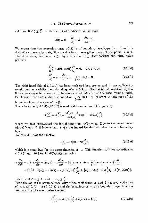
3.2. The Formal Approximation 233
valid for 0 < ~ < x while the initial conditions for 9 read _ - ~ - ~
d9 dw ~(0) = O, _-7-; = ~ - -;:(0). aq ~Yb"
We expect that the correction term 69(~) is of boundary layer type, i.e. 9 and its derivatives have only a significant value in an ~-neighbourhood of the point x - 0. Therefore we approximate 9(~) by a function v(~) that satisfies the initial value problem
dv (10.3.6) d ~ (0, ~ ( o ) ) d~ 2 + a = 0 , 0 < ~ < o o
dv dw d ---7 = ~ - ax----7-(O) lim v(~) = 0. (10.3.7)
~--~oo
The right-hand side of (10.3.5) has been neglected because a and b are sufficiently regular and w satisfies the reduced equation (10.3.3). The first initial condition 9(0) = 0 has been neglected since 69(0) has only a small influence on the initial value of u(x). Furthermore we have added the condition lim v ( ~ ) = 0 in order to take care of the
~--~oo boundary layer character of v(~). The solution of (10.3.6)-(10.3.7) is readily determined and it is given by
~'(o)- v(r = v(~)~ = a(o,,~) - - exp [-- a(O, oOX], (10.3.8)
C
where we have substi tuted the initial condition w(0) - a. Due to the requirement a(x, u) >_ a0 > 0 it follows that v(X) has indeed the desired behaviour of a boundary layer. We consider now the function
~(x) -- w(x) + ev(X), (10.3.9) e
which is a candidate for the approximation of u. This function satisfies according to (10.3.3) and (10.3.6) the differential equation
d2 ~ d~t d2 w ~ x 2 + a(x, ~t) -~x + b(x, ~) - ~-~x 2 + {a(x, w(x) + cv(X))~ - a(x, w(x)) } dWdx
dv q- {a(r w ( ~ ) + cv(~)) - a(0, w(0))}~-~ + {b(x, w(x) q-- cv(~)) - b(x, w(x)) },
X valid for 0 < x _ < X and 0 < ~ < - / . With the aid of the assumed regularity of the coefficients a and b (consequently also of w �9 C2[0, X] -see (10.3.3)-) and the behaviour of v as a boundary layer function we obtain by the mean value theorem
d2fi dfi ~ + a(x, ~) ~ + b(x, ~) = O(~) (10.3.10)
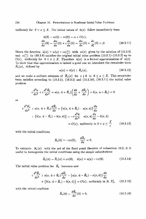
234 Chapter 10. Perturbations in Nonlinear Initial Value Problems
uniformly for 0 < x < X. The initial values of fi(x) follow immediately from
~(o) = ~(o) + ~ ( o ) = ~ + o(~), dft dw dv dw dv d---~(O) = ~x (O) + S-~x(O ) = ~x (O) + -~(0) = t3. (10.3.11)
Hence the function fi(x) = w(x) + r with w(x) given by the solution of (10.3.3) and v(~) by (10.3.8) satisfies the original initial value problem (10.3.1)-(10.3.2) up to O(e), uniformly for 0 < x < X. Therefore ~(x) is a formal approximation of u(x). To show that this approximation is indeed a good one we introduce the remainder term Re(x), defined by
u(x) = f i (x)+/~e(x) , (10.3.12)
and we make a uniform estimate of /~e(x) for e $ 0 in 0 < x < X. This remainder term satisfies according to (10.3.1), (10.3.2) and (10.3.10), (10.3.11) the initial value problem
~-g-~ + ~ ~ + a ( ~ , a+&) ~ + a~ ] +b(~, a + & ) = o
o r
d2 Re dx 2
+ a(x, ~t + Re) dRe d~ + {a(x, fi + Re) - a(x, fi)} dx
d2~t -- a(x, ft) d~t + {b(~, ~ + & ) - b(~, ~1 } = - ~ d - ~ ~ - b(~, ~1
X = O(e), uniformly in 0 < x _ - -
6 (10.3.13)
with the initial conditions
d / ~ Re(O) = -ev(O), dx = O.
To estimate /~e(x) with the aid of the fixed point theorem of subsection 10.2, it is useful to homogenize the initial conditions using the simple substitutions
h~(~) = R~(~) + ~,(o), ~(~) = ~(~) - ~,(o). (10.3.14)
The initial value problem for /~e becomes now
d2/~E d/~e d~ c ~ + a ( x , fi + / ~ e ) ~ + {a(x, ~ + he) - a(x,~)}~--xx
+ {b(x, ~t + R e ) - b(x, fi)} = O(e), uniformly in [0, X], (10.3.15)
with the initial condition dh~
h~(o) = - - ~ (o) = 0; (10.3.16)
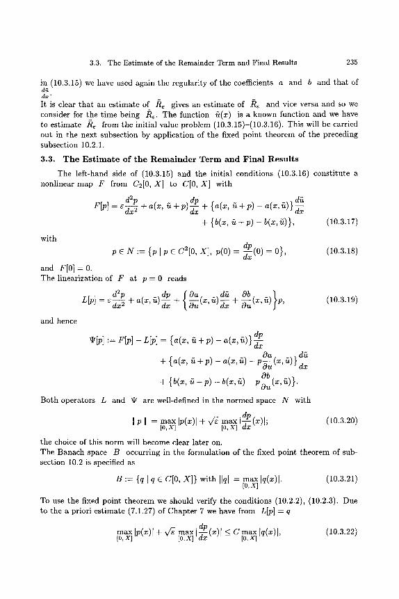
3.3. The Estimate of the Remainder Term and Final Results 2 3 5
in (10.3.15) we have used again the regularity of the coefficients a and b and that of d ~ dx"
It is clear that an estimate of / ~ gives an estimate of / ~ and vice versa and so we consider for the time being /~ . The function ~(x) is a known function and we have to estimate / ~ from the initial value problem (10.3.15)-(10.3.16). This will be carried out in the next subsection by application of the fixed point theorem of the preceding subsection 10.2.1.
3.3. T h e E s t i m a t e of t h e R e m a i n d e r T e r m a n d F ina l R e s u l t s
The left-hand side of (10.3.15) and the initial conditions (10.3.16) constitute a nonlinear map F from C2[0, X] to C[0, X] with
d2p dp d~z F [ p ] - e ~ x 2 4- a(x, u 4-P)dxx 4- {a(x, ~ 4 - p ) - a ( x , ~ ) } ~ x
4- {b(x, ~ 4- p) - b(x, ~)}, (10.3.17)
with @
p E N := {PIP E C2[0, X], p(0) = ~x(0) = 0},
and F[0] = 0. The linearization of F at p - - 0 reads
d2p dp { Oa dCt Ob } LiP] = c--~x 2 + a(x, ~t) ~ + ~ (x, ~) dxx 4- ~u(X, u) p,
and hence
(10.3.18)
(10.3.19)
ap �9 ~] "- F[p] - Lip] - { a(x, ~z + p) - a(x, ~t) }
Oa d5 + {a(x, Ct + p) - a(x, ~) - p-~u(x, ~z)} dx
Ob + {b(x, ~z + p) - b(x, ~) - p-~u(X, ~z)}.
Both operators L and ~I' are well-defined in the normed space N with
I P I - max Ip(x)l + v ~ max I dp (10.3.20) t0,xl t0,xl ~(~)1;
the choice of this norm will become clear later on. The Banach space B occurring in the formulation of the fixed point theorem of sub- section 10.2 is specified as
B := { q l q E C[0, X]} with Ilqll- max Iq(x)l. (10.3.21) [0,x]
To use the fixed point theorem we should verify the conditions (10.2.2), (10.2.3). Due to the a priori estimate (7.1.27) of Chapter 7 we have from Lip] = q
max Ip(x)l + v/~ max I dp -7-(x)l < C max Iq(x)l, (10.3.22) [o,z] [o,x] r - - [ o , x ]
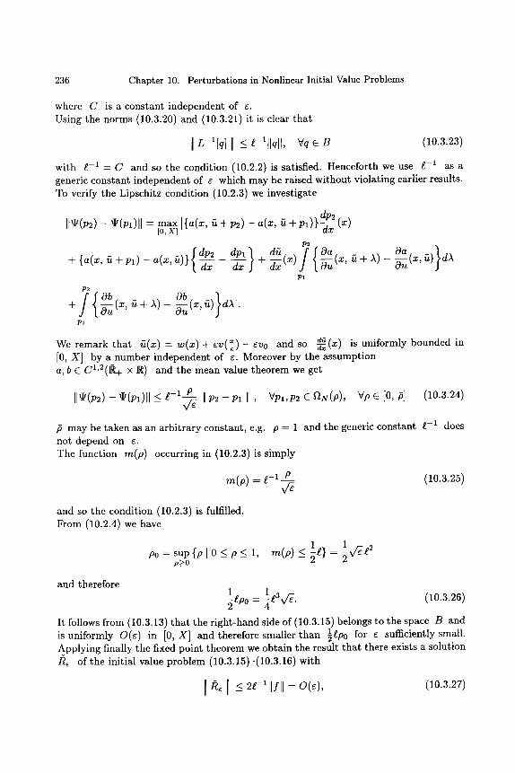
236 Chapter 10. Perturbations in Nonlinear Initial Value Problems
where C is a constant independent of e. Using the norms (10.3.20) and (10.3.21) it is clear tha t
I L-l[q] [ _< e-lllqll, Vq ~ B (10.3.23)
with ~-1 = C and so the condition (10.2.2) is satisfied. Henceforth we use s as a generic constant independent of e which may be raised without violating earlier results. To verify the Lipschitz condition (10.2.3) we investigate
@2 II~(p2) - ~(px)ll - max I{a(x, ~z + p2) - a(x, (z + pl)}-d-x-x (x)
[0,x] P2 {dp2 dpl} du :{Oa(x,~4-~)Oa(x,~)}d~
4- {a(x, ~ 4- PI) - a(x, fi)} dx dx 4- '~x (x) ~ Pi
P2
+ ~ ( x , ~ + a) - (x, r~) a~ I Pi
x d4 We remark tha t fi(x) = w(x) + ev(7 ) - evo and so ~-d(x) is uniformly bounded in [0, X] by a number independent of e. Moreover by the assumption a, b E C1 '2( ]~ x R) and the mean value theorem we get
II~(p2)- ~(px)ll < ~-1 p _ -~ Ip2 - p l I, ~ p l , p 2 e ~"~N(P), Vp E [0, p] ( 1 0 . 3 . 2 4 )
,5 may be taken as an arbi t rary constant, e.g. /5 = 1 and the generic constant s does not depend on e. The function m(p) occurring in (10.2.3)is simply
r e ( p ) = I. - i - p (10.3.25) v~
and so the condition (10.2.3) is fulfilled. From (10.2.4) we have
p 0 = s u p { p I 0 _ < P _ < I, p_>o
1 ~2 re(p) ___ ~} = ~v~
and therefore l ~ p 0 = l~3%/fE. (10.3.26)
It follows from (10.3.13) tha t the r ight-hand side of (10.3.15) belongs to the space B and is uniformly O(e) in [0, X] and therefore smaller than �89 for e sufficiently small. Applying finally the fixed point theorem we obtain the result tha t there exists a solution ~ R~ of the initial value problem (10.3.15)-(10.3.16) with
I k. I -< 2 - llfll = o ( , ) , (10.3.27)
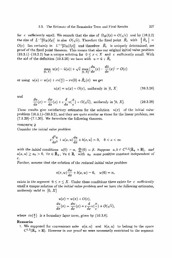
3.3. The Estimate of the Remainder Term and Final Results 237
for ~ sufficiently small. We remark that the size of ftB(t.p) = O(X/~) and by (10.2.2)
the size of L-l[FtB(lp)] is also O(v~) . Therefore the fixed point / ~ with I / ~ [ -
O(~) lies certainly in L-I[~B(ip)] and therefore k~ is uniquely determined; see proof of the fixed point theorem. This means that also our original initial value problem (10.3.1)-(10.3.2) has a unique solution for 0 < x < X and ~ sufficiently small. With the aid of the definition (10.3.20) we have with u = ~ + / ~
max I du d~ max lu(x) - ~(x)l + V~ -:-(x) - - :-(x)l = O(~) [0,z] [0,x] g x - -
or using u(x) -- w(x) + ev(-~) - ev(O) + ke(x) we get
u(x) = w ( x ) + O(e), uniformly in [0, X] (10.3.28)
and du dw d x dx(X) - -~X-X (x) + r + O(~/~), uniformly in [0, X]. (10.3.29)
These results give satisfactory estimates for the solution u(x) of the initial value problem (10.3.1)-(10.3.2), and they are quite similar as those for the linear problem, see (7.1.29)-(7.1.30). We formulate the following theorem.
THEOREM 2
Consider the initial value problem
d2u du r 2 + a(x, u) + b(x, u) - 0, 0 < x < o o
du with the initial conditions u(O) = a, -g~(O) = 3. Suppose a, b C C1'2(1~ • R), and a(x, u) >_ ao > O, Vx E IR+, Vu C N, with ao some positive constant independent of
Further, assume that the solution of the reduced initial value problem
a(x, w) dw + b(~, w) = o, ~ ( o ) - ~,
exists in the segment 0 <_ x <_ X . Under these conditions there exists for e sufficiently small a unique solution of the initial value problem and we have the following estimates, uniformly valid in [0, X]
~(~) = ~ ( ~ ) + o(~), du dw -c d v(X d---~(x) = ~ ( x ) + ~ ~) + O(v/~),
where ev(~) is a boundary layer term, given by (10.3.8).
R e m a r k s
1. We supposed for convenience sake a(x, u) and b(x, u) to belong to the space C1'2(1~ • 1~). However in our proof we were necessarily restricted to the segment
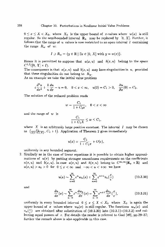
238 Chapter 10. Perturbations in Nonlinear Initial Value Problems
0 < x _ X < X0, where X0 is the upper bound of x-values where w(x) is still regular. So the semibounded interval ~ may be replaced by [0, X]. Further, it follows that the range of u values is now restricted to an open interval I containing the range Rw of w:
I ~ n ~ - {y c R I3= e [0, x ] with y = w(x)}.
Hence it is permit ted to suppose that a(x,u) and b(x,u) belong to the space C1'2([0, X] X I).
The consequence is that a(x, u) and b(x, u) may have singularities in u, provided that these singularities do not belong to Rw. As an example we take the initial value problem
d2u 1 du Ou Ed~x 2 -~--udxx -~-zt=0, 0 < x < (:x:), u(0) = C 1 > 0, ~x(0) = C 2 .
The solution of the reduced problem reads
C1 w - - 0 < x < c x )
1 + Clx'
and the range of w is C1 <w~_C1,
1 + C 1 X -
where X is an arbitrarily large positive constant. The interval I may be chosen as (2(l+C1x),Cx C1 + 1). Application of Theorem 2 gives immediately
C1 u ( ~ ) = ~ + o ( ~ ) ,
1 +Clx
uniformly in any bounded segment. 2. Similarly as in the case of linear equations it is possible to obtain higher approxi-
mations of u(x) by putt ing stronger smoothness requirements on the coefficients a(x, u) and b(x, u). In case a(x, u) and b(x, u) belong to C ~,~176 (]~+ x R) and a(x,u) > a 0 > 0 for 0 < x < o o and - c ~ < u < + o o we have
dO dO U(X) ~ ~ 6nwn(X ) + ~ 6nTlvn(X-- ) (10.3.30)
n=O n=O
and du dO dwn do dvn x
--~X (X) -~- ~ 6n+1 "-~X ( C , n=0 n=0
(10.3.31)
uniformly in every bounded interval 0 < x < X < X0 where X0 is again the upper bound of x values where wo(x) is still regular. The functions w,.,(x) and v,,(~) are obtained after substi tution of (10.3.30) into (10.3.1)-(10.3.2) and col- lecting equal powers of e. For details the reader is referred to Geel [49], pp.29-37; further the remark above is also applicable in this case.
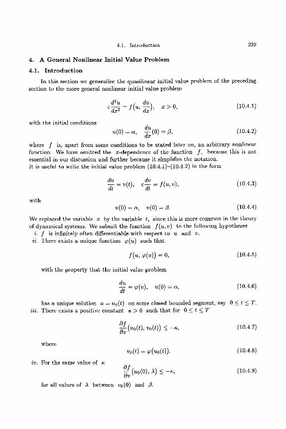
4.1. Introduction 239
4. A G e n e r a l N o n l i n e a r Ini t ia l Va lue P r o b l e m
4.1. I n t r o d u c t i o n
In this section we generalize the quasilinear initial value problem of the preceding section to the more general nonlinear initial value problem
d2u du r = f (u , ~xx), x > 0, (10.4.1)
with the initial conditions du
u(0) = a, ~xx(0) =/3, (10.4.2)
where f is, apart from some conditions to be stated later on, an arbitrary nonlinear function. We have omit ted the x-dependence of the function f , because this is not essential in our discussion and further because it simplifies the notation. It is useful to write the initial value problem (10.4.1)-(10.4.2) in the form
du dv dt = v(t), E-~ = f (u , v), (10.4.3)
with u(0) = a, v(0) =/3. (10.4.4)
We replaced the variable x by the variable t, since this is more common in the theory of dynamical systems. We submit the function f (u , v) to the following hypotheses
i. f is infinitely often differentiable with respect to u and v. ii. There exists a unique function ~(u) such that
f ( u , ~o(u)) = 0, (10.4.5)
with the property that the initial value problem
du d---t- = ~(u), u(0) - a, (10.4.6)
has a unique solution u = uo(t) on some closed bounded segment, say 0 _< t _< T. iii. There exists a positive constant ~ > 0 such that for 0 _< t _< T
of av( O(t), < (10.4.7)
where
iv. For the same value of
vo(t) = ~(uo(t)) . (10.4.8)
of Ov (u0 (0), < (10.4.9)
for all values of )~ between v0(O) and ft.
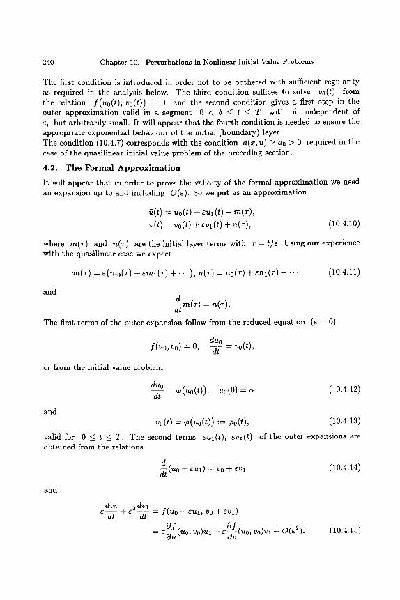
240 Chapter 10. Perturbations in Nonlinear Initial Value Problems
The first condition is introduced in order not to be bothered with sufficient regularity as required in the analysis below. The third condition suffices to solve vo(t) from the relation f (uo( t ) , vo(t)) = 0 and the second condition gives a first step in the outer approximation valid in a segment 0 < 5 <_ t <_ T with 5 independent of e, but arbitrarily small. It will appear that the fourth condition is needed to ensure the appropriate exponential behaviour of the initial (boundary) layer. The condition (10.4.7) corresponds with the condition a(x, u) > a0 > 0 required in the case of the quasilinear initial value problem of the preceding section.
4.2. T h e F o r m a l Approximation
It will appear that in order to prove the validity of the formal approximation we need an expansion up to and including O(e). So we put as an approximation
ft(t) = uo(t) + eul (t) + re(T), ~(t) = vo(t) + ~vl(t) + n(~), (10.4.10)
where m(T) and n(~-) are the initial layer terms with T = t /e. Using our experience with the quasilinear case we expect
m(,) = ~(~o(-) + ~ml(~) + . . . ) , ~(~) = ~o(:) + ~ ( - ) + . . (10.4.11)
and
m(r ) = n(r) .
The first terms of the outer expansion follow from the reduced equation (e - O)
duo f (uo, Vo) -- O, dt = vo(t),
or from the initial value problem
duo dt
= qO(uo(t)), u o ( 0 ) - a (10.4.12)
and vo(t) = ~o(uo(t)) "= ~oo(t), (10.4.13)
valid for 0 _< t _< T. The second terms eUl (t), evi (t) of the outer expansions are obtained from the relations
d d-~(uo + e U l ) = v0 n t- e V l (10.4.14)
and
dvo ~2 dvl ~ - ~ + - ~ = f (uo + ~=1, .0 + ~Vl)
Of Of = ~ ( ~ o , ~o)u~ + ~ ( u o , ~o)~ + o ( ~ ) . (10.4.15)
4.2. The Formal Approximation 241
We do not calculate ul(t) , vl(t) from (10.4.14) and (10.4.15), but from the approxi- mation
dvo Of Of ] g--~ -- ~ ~U (U0, V0)U 1 -~- ~V (U0, V0)V 1j , (10.4.16)
making an error of only O(e2). Hence we get
dvo e2 dvl - C - ~ -Jr- W -- f (uO nt- CUl, VO n t- ~Vl) n t- O(C2), (10.4.17)
uniformly in [0, T]. Therefore Ul, Vl satisfy the equations
d u l = ~ l ( t )
dt
and Of - l dvo Of Of
V 1 (t) -- (~V (U0, V0) ) --~-- (t) -- (~--~ (U0, V0) ) (~V (U0, V0))--lul(t).
With the aid of the relation
Of Of d~ (~o, vo) + -a-(~o, ~o) , . - (~o) = o, Ou u v auo
we obtain for U 1 (t) the differential equation
dul dt
d~ Of -1 dvo du0(~0)~l + (~(~0,v0)) dt (10.4.18)
with the still unknown initial condition
ul(0) = - too(0). (10.4.19)
The initial condition is to be determined from the initial layer analysis below. The solution of this initial value problem gives Ul (t) and consecutively the function vl(t) follows from (10.4.18)
du l d~ Of - 1 dvo v~(t) = -~ - ( t )= ~o(~O)~( t )+ (~(~0,~o)) -~/-(t). (10.4.20)
The pair (uo+eul, vo+evl) satisfies the differential equations (10.4.3) up to O(e 2) uni- formly in [0, T], but the initial conditions (10.4.4) are not fulfilled. In particular we have
d d uo(O) + eUl (0) = a + eUl (0) and vo(O) + eVl (0) = uo(O) + e ~ u l (0).
242 Chapter 10. Perturbations in Nonlinear Initial Value Problems
This error is corrected by the introduction of the initial layer t e r m s ~mO(T) and nO(T) + enl (T) satisfying in their turn the initial conditions
d d mo(0) - -eUl (0), no(0) -- ~ - ~-~uo(0) --/~ - vo(0), nl (0) -- -~-~Ul (0) -- -Vl (0).
(10.4.21) Further we have
~ e m o ( ) = -d--~rmO(T) -- no(T). (10.4.22)
Let no(T) + ~n 1 (T) satisfy the equation
dno dnl dT + e--~-T = f(Uo + ~Ul + emo, Vo + eVl + no + enl) -- f (uo + eUl, Vo + eVl)
dvo e2 dvl : f ( t t 0 n t. CUl n t. ~ m 0 , v 0 + Ev 1 + n o -~- C n l ) -- E - - ~ - -- - - ~ -~- O ( ~ 2 ) , (10.4.23)
or with the aid of the mean value theorem
dno dnl dT dT
f (Uo + eUl + emo, Vo + -CVl + no + -ca1) -- f (Uo + eUl + ~mo, Vo + eVl + no)
+ : ( u o + ~u: + ~..o. ~o + ~v~ + no) - f ( u o + ~ : . ~o + ~ : ) =
o f e O--vv (uo + eUl + emo, vo + g'Vl + 'r/,O -t- g '~91'nl) ' r t l
o ] +e~-~u (uo + eUl + e~92mo, vo + eVl + ~92no)mo
o.f + O r (u0 + ~Ul + gz92mo, Vo ~- ~Vl + ~2no)no,
where Zgl and ~2 are functions of T with 0 < Z91(T), Z92(T) < 1. Expanding the right-hand side with respect to e we get
dno dT
_ _ o f (uo(O), vo(O)+ ,h(~-)no(~-)) �9 no(~-), - T > o Ov
(10.4.24)
and dnl dr
= N(T), T > 0 (10.4.25)
with N(T) the complicated expression
N(T) Of Of = ~ (~o(O), ~o(O)+ ~o(~))~1(~)+ ~ (uo(O), vo(O)+ 0~(~)~o(~))mo(~)
1 { O f + - (uo(~) + ~Ul(~) + ~o~(~)mo(~), ~o(~) + ~v~(~) + o~(~)~o(~))
} Ov (uo(O), vo(O)+ 0,2(r)no(r)) no(-) . (10.4.26)
4.2. The Formal Approximation 243
The initial values for no(T) and nl(T) are given by (10.4.21). Solving the initial value problem for no we use now the hypothesis (10.4.9), which gives that the factor of no(T) in the right-hand side of (10.4.24) is negative whenever the value of v0(0) § 02 (~')n0 (T) is between v0(0) and /3. This is certainly the case for ~- = 0 and so nO(T) is monotone till nO(T) vanishes; nO(T) decreases to zero whenever /3 > v0(0) and it increases to zero whenever ~ < v0(0). Hence we have
Ino(~)l =_< I~- ~o(0)1 exp[--~T], 0 _< T < (x~, (10.4.27)
and so nO(T) has the right assymptotic behaviour as required in an initial boundary layer. The other initial layer function mO(T) follows from (10.4.22) and we have
o o
mO(T) -- -- / no('r')dT'. (10.4.28)
T
Also too(T) has the right asymptotic behaviour for ~- --+ r and moreover
OO
m0(0) = - / ~0(~')~' , (10.4.29)
0
and the still missing initial condition for ul(t), see (10.4.19), is now known. It is in general difficult to get an explicit expression for toO(T) and nO(T) and therefore we have to be content with their qualitative behaviour as represented by (10.4.27) and (10.4.28). Finally we have to investigate the function nl (T) and in particular its asymptotic be- haviour. Using again the condition (10.4.9), the boundary layer behaviour of too(T) and no(T) and the regularity of the function f we obtain from (10.4.25)-(10.4.26) that also nl(T) has the right boundary layer character with
nl (T) = O(exp[--~(1 -- 5)T]), (10.4.30)
where 5 is an arbitrarily small positive number independent of r this number is to be introduced because there appears in N(T) after a further expansion with respect to r terms like "rno(T). We consider now the expressions
~(t) -~ r ) § ~Ul(t) § ~mO(T)
and (10.4.31)
~(t) = ~0(t) + ~v~(t)+ ~0(~) + ~n~(~).
On account of their construction, see (10.4.15) and (10.4.23), they satisfy the initial value problem
d~ d---t = ~(t) - ~ n l (T)
d~ e~-~ = f(~, ~ ) + O(e2), uniformly in [0, T],
244 Chapter 10. Perturbations in Nonlinear Initial Value Problems
with the initial conditions fi(0) = (~, ~(0) = f~. (10.4.32)
Hence (10.4.31) constitutes a [ormal approximation of the solution (u, v) of our initial value problem (10.4.3)-(10.4.4). To prove that (fi, ~) is indeed a good approximation we put
u(t) = fi(t) + R(t), v(t) = ~(t) + S(t), (10.4.33)
where (R, S) is a solution of the initial value problem
dR du dfi ~t = d t d t = ~( t ) - (~( t ) - ~,,~(~)) = s ( t ) + ~(~)
and dS ( d v d ~ )
e - ~ -- e dt dt - f (fi-l- R' ~ + S) - f (~t' ~) -4- O ( e 2)
with R(0) - S(0) = 0. We now make the irrelevant change
R(t) = R(t) + E nl (--~)dt' = R(t) + E 2 nl (T)dT
0 0
= k ( t ) + o ( ~ ) ,
and this gives for the remainders /~(t) and S(t) the initial value problem
(10.4.34)
dk "- S~
dt dS
uniformly for 0 < t < T while the initial conditions are
(10.4.35)
/~(0) ---- S(0) - 0. (10.4.36)
In the next subsection we derive from this initial value problem an a priori estimate for /~(t) and S(t), which validates the formal approximation (10.4.31).
4.3. T h e E s t i m a t e of t h e R e m a i n d e r T e r m s a n d t h e F i n a l R e s u l t
We use again the fixed point theorem of section 2. Inserting the first equation of (10.4.35) into the second we get
d2/~ d/~ ~ - ~ - f (~ + R, ~ + - ~ ) + f(~t, ~) = O(~2), (10.4.37)
uniformly in 0 _< t _< T, with the initial conditions
k(0) = dk -~ - (0) -- 0. (10.4.38)
4.3. The Estimate of the Remainder Terms and the Final Result
The nonlinear operator F is defined by
d2p dp F[p] = r - f(~2 + p, ~ + -~) + f(~2, fi),
with F(0) - 0. As p- and q-spaces we take again
dp N "= {p E C2[0, T], p(0) - ~-~(0) = 0},
with norm
and
I p l - m a x Ip(t)l + v ~ m a x I dp tO, T] [0, T] ~(t)l,
245
(10.3.20)
and
d2p Of Of dp L[p] = e dt 2 O~z (~z, 9)p - ~ v (~Z, ~) -d-[ (10.4.39)
dp Of Of dp (10.4.40) ~ [ P ] - - f ( ~ + P ' ~ + ~- ) + f (~ ' ~) + 0--~(~' ~)P + ~ - ( ~ ' ~) d--t-"
To apply the fixed point theorem of section 2 we have to check the conditions (10.2.2) and (10.2.3). Due to the a priori est imate (7.1.27) of Chapter 7 we have from L~)] = q
I p(t) I _< Cllqll where C is a generic constant independent of e. Therefore
I L-~[q]l < e-lllqll, Vq e B,
with ~ = C -1 and condition (10.2.2) is fulfilled. To verify the Lipschitz-condition (10.2.3) we investigate
I]~[P2]- ~[pl]ll =
dp2 dpl ~ _ Of max f(~z+p2 v+ ) - f ( f t + p l v+ dt / -~u(~z,v)(p2-pl) E0, T] ' ~ '
Of ( dp2 dpl ) dp2 ] _ dpl = m a x f (zt + p2, v -4- f (zt + pl v-f- ) Ov (ft, ~) - dt [0, T] dt " '
dpl ~ _ Of dpl ~ ( dp2 dpl ) Of .u+pl( v+ (P2 P l ) - (~2+pl, v + O u ' --~ " -~v - ~ " d t d t
dpl Of Of dpl Of +{Ouu0f (g + Pl, v + - -~ ) - Ouu (u' ~) } (P2 - Pl) + { ~vv (72 + Pl ' v + ~ ) - Ovv (~2, ~) }
(dp2 dpl) dt dt "
where
B " - {q e C[0, T]}, with norm I lq l= max Iq(t)l. (10.3.21) [0,T]
The operator F is splitted as before in its linear part L and the remainder 9 . Hence
F~] = L~] + ~ ] ,
246 Chapter 10. Perturbations in Nonlinear Initial Value Problems
Using Lagrange's remainder term it follows with the aid of (10.3.20) that
II~#[p2] - ~[p~]l l _%< e-1/9 [P2 - Pl I , (10.4.41)
valid for all P2 and pl in any ball ~N(P) with p E [0, is]; e -1 is a generic constant and t5 may be any positive constant, e.g. /5 = 1. The function re(p) occurring in (10.2.3) is now
re(p) - e -~ ~, E
and condition (10.2.3) is fulfilled. From (10.2.4) we have
PO = sup{p 10 < p < 1, m(p) < ~l.} = 2~. 2 p___o
and therefore l~po = ~e~3.
Since the right-hand side of (10.4.37) is 0(~ 2) we may apply the fixed point theorem and we get finally the result
I k l = (10.4.42)
It is clear that we needed a formal approximation up to O(~2), otherwise the right-hand side of (10.4.37) would have been O(e) and we could not apply the fixed point theorem. The result is that /~(t) exists uniquely and we have the estimate
max IR(t)l + v/~max I d h [0,r] [0,r] -~-I = o ( e 2 ) ,
and this gives u ( t ) : Uo(t ) -4- ~U 1 (t) -~- ~mO(T ) -Jr- O(E2), (10.4.43)
uniformly in [0, T]. dk dn 0 (6 )= Moreover we have also dh = O(~3/2) uniformly in [0, T]. However -~- - -~-+
du dfi dt dt+ O(r and therefore
du d t = vo(t) + no(T) + O(~), uniformly in [0, T]. (10.4.44)
Collecting our results we have the following theorem
THEOREM 3 The initial value problem
d2u du r - f (u, -~-) , O < t < o o
4.3. The Estimate of the Remainder Terms and the Final Result 247
with the initial conditions u(O) = a and du -~(0) -- ~ has under the hypotheses i-iv, stated in subsection 10.4.1, a unique solution in the segment 0 <_ t <_ T. Moreover the following approximations are uniformly valid in [0, T]
t u(t) -- uo(t) + Cul(t) ~- r (~) -~- O(~2),
du duo t ) + O(e), d--~(t) = --d-~(t) + no(~
where the outer expansion terms uo(t), ul( t ) and vo(t) are determined by (10.4.12), (10.4.13), (10.4.18) and the initial layer terms e m o ( t ) and n o ( t ) by (10.4.21), (10.4.24) and (10.4.28).
E x a m p l e We illustrate the theory with the famous example of the van der Pol equation ,
which reads d2u du
r + (u 2 - 1) + u = 0. (10.4.45)
This equation gives so-called relaxation oscillations which are periodic solutions charac- terized by a change in t ime al ternately slow and fast. We write (10.4.45) in the equivalent form of a system, viz.
d u ~ v
dt dv
e-dt = ( 1 - u2)v - u = ( 1 - u 2 ) ( v - U
1 - u 2 )" (10.4.46)
Taking initial conditions u(0) - a, v(0) = p we get as a first approximat ion valid outside the initial layer
U0 v0 = 1 - u~'5 u0 ~: +1, (10.4.47)
with
and integration yields
We put
duo uo dt - 1 - u 2' u 0 ( 0 ) = a ,
t
1 3 f 1 3 uo(t) - g(u0( t ) ) = J uo(t')dt' + a - g a . 0
t
- + f u(,')d,' : 0
and we get as another equivalent system
dw dt - u ,
du !u3 -~- W e~-~ = u - 3
(10.4.48)
(10.4.49)
(10.4.50)
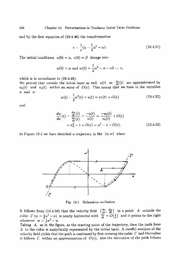
248 Chapter 10. Perturbations in Nonlinear Initial Value Problems
and by the first equation of (10.4.46) the transformation
v -- - ( u - u 3 + w). (10.4.51)
The initial conditions u(0) = a, v(0) - ~ change into
u ( 0 ) = a a n d w ( 0 ) - ~ a 3 - a + r
which is in accordance to (10.4.49). du We proved that outside the initial layer as well u(t) as ~-(t) are approximated by
uo(t) and vo(t) within an error of O(r This means that we have in the variables u and w
~ ( t ) - ~ - u ~ ( t ) + ~ ( t ) - ~ v ( t ) = . 1
0(~) (10.4.52)
and
dw -~t (t) - u ( t ) - u o ( t ) ~- 0(~) du (t) = ~ . . . . . - ~ ( t ) ~(t) ~o(t)
= u 2 - 1 + 0 ( ~ ) = u 2 - 1 + 0 ( ~ ) . (10.4.53)
In Figure 10.1 we have sketched a trajectory in the (u, w) plane
/ : 7
fY
D ( /
/ , g
%
%
%
,'e J
J A /
i / ~
Fig. 10.1 Relaxation oscillation
It follows from (10.4.50) that the velocity field (du dw ~-, -~-) in a point A outside the
cubic C (w - �89 3 - u) is nearly horizontal with -~-d~ _ O(~) and it points to the right 1 3 whenever w > 5u - u .
Taking A, as in the figure, as the starting point of the trajectory, then the path from A to the cubic is analytically represented by the initial layer. A careful analysis of the velocity field yields that the path is continued by first crossing the cubic C and thereafter it follows C within an approximation of O(c); also the derivative of the path follows
4.3. The Estimate of the Remainder Terms and the Final Result 249
the derivative of C within the approximation of O(r see (10.4.52) and (10.4.53). 1 3 Whenever w < 5u - u and A lies at the other side of the cubic there is no crossing and
the path follows again the cubic. This is all in accordance with the theory of this and the preceding section, as long as o ( ( 1 - u 2 ) v - U) "-- 1 - u 2 < -n . So the theory holds as long as the path has not reached the "critical" value u = 1, and the problem arises how to pass the neighbourhood of the "critical" point C (1, - 2). Analyzing the location of the trajectory in this neighbourhood it can be shown that the trajectory contains a
2 W* -2 /3 . point (u*,w*) at a d i s t anceofa t least 0(r 1/3) from ( 1 , - 5 ) and with <
d~ becomes O (r ~) and so Inserting these coordinates into (10.4.50) one obtains that -~- 2 (u(t), w(t)) gets enough impetus to leave the neighbourhood of (1, - 5 ) and the path
is continued nearly horizontally in the direction of D and the story can be repeated again. The velocity field allows to apply the Poincar~-Bendixson theorem, see e.g. [60, Ch.II] and so there exists a periodic solution. The trajectory of this periodic solution lies in a
1 3 2 for neighbourhood of a closed curve defined by w = 5u - u for 1_<u_<2, w = - 5 l U3 2 for - 1 < u < 2. The - 2 < u < 1, w : 5 - u for - 2 < u < - 1 and w = +5 - -
distance of the periodic trajectory to this curve approaches zero for r $ 0 and it is of lU3 order O(r along the branches of the cubic w = 5 - u. There exists much literature
on the van der Pol equation and we refer the reader to Wasow [139, p.301] and O'Malley [112, p.62]. Also should be mentioned the work by Troesch and Urlacher [133], who gave a fine analysis of the behaviour of the trajectories in the neighbourhood of the critical
2 points (+1, TS). This paper is one of the first of many interesting publications, where nonstandard analysis is used in singular perturbation theory [101,133, 134, 17, 4, 136]; see also M. Canalis-Durand, Solution formelle Gevrey d'une ~quation singuli~rement perturb~e; Asymptotic Analysis, 8, (1994). Finally we remark that we discussed in section 3.5 of Chapter 5 the equation
d2u d u + r 2 - 1 ) - - . + u - 0 , t > 0 , 0 < r
dt---- ~ (10.4.54)
This equation becomes with t = r the counterpart of equation (10.4.45), namely
1 d2u du r dT----- ~ -~- (U 2 -- 1)~TT + U = 0, T > 0, 0 < r << 1. (10.4.55)
We have shown in section 3.5 of Chapter 5 that the solution of (10.4.54) is of the form
u(t) = 2(1 - A e - a ) -�89 cos(t + ~0) + O(r
and the influence of the perturbation r 2 1) du is only observable after a long time. - -~ _ d 2 u is This is in contrast with the solution of (10.4.45), where the perturbation ed--~
immediately observable in the large horizontal velocity field.
250 Chapter 10. Perturbations in Nonlinear Initial Value Problems
5. Q u a s i l i n e a r Init ia l Value P r o b l e m s w i t h a S i n g u l a r P e r t u r b a t i o n of S e c o n d O r d e r H y p e r b o l i c T y p e
5.1. I n t r o d u c t i o n
We discuss the singular initial value problem
EL2[u]+Lliu]=O, (x,t) e D - { - ~ < x < + c r t > 0 } ,
with
and
02u c2(x, t) 02u L2[u] = Or---- ~ - Ox 2
(10.5.1)
Ll[u] = a(x, t, u) Ou Ou Ox + b(x, t, u ) -~ + d(x, t, u). (10.5.2)
The initial conditions are given by
Ou u ( x , O ) - f(x) , -~(x) = g(x), - c r < x < +cr (10.5.3)
To avoid tedious book-keeping we assume for convenience a(x, t, u), b(x, t, u), d(x,t ,u) C C ~ ( D x R), c(x,t) c C~176 f(x) , g(x) E C ~ ( R ) and in addition we require similarly as in Chapter 9, section 3
i. c(x, t) > 0 in D, c(x, t) uniformly bounded in any strip {(x, t)} with - cr < x < +cx), 0 < t < T *
ii. b(x,t,u) > O in D x R , iii. la(x, t, u)l < b(x, t, u)c(x, t) in D x R. The last condition ensures the timelike character of the subcharacteristics, see Ch.9, section 2. As in all preceding sections we start with the construction of a formal approx- imation consisting of the sum of the solution of the reduced problem with 6 - 0 and a correction accounting for the second initial condition. Consecutively we formulate the initial value problem for the error R~ and we give an a priori estimate using again the fixed point theorem which yields also the unique existence of R~ and by this the unique existence of the solution u of the initial value problem (10.5.1)-(10.5.3). Related initial value problems with more space dimensions have been studied by Genet and Madaune [51], [102]. They discussed a nonlinear differential equation of the type
02u -- As) + a(x, t)Ou n Ou e(-O--~ -~ + E bk(x,t) ~ + c(x, t)u + F(u) = f (x , t ) k- -1
with (x, t) E ~ • ~ C R '~. The a priori estimates and approximations of u obtained by these authors are estimates and approximations in the L v norm.
5.2. T h e F o r m a l A p p r o x i m a t i o n
A formal approximation of our initial value problem (10.5.1)-(10.5.3) is given by
t (10.5.4) ~o(~, t) = ~o(~, t) + ~ o ( ~ , ~),
5.2. The Formal Approximation 251
where w0(x,t) satisfies the reduced problem
Owo Owo a(x,t, wo)-~x + b(x,t, w o ) - ~ + d(x,t, wo) - O, - o c < x < + o c , t ; > 0
To(x, O) - f(x), - c ~ < x < +c~, (10.5.5)
t while evo(x, -i) = evo(x, T) is the boundary layer correction. This term is a solution of the boundary value problem
02vo Ovo a~---~ + b(~, o, wo(~, o ) ) - ~ - o, ~- > o
Ovo Owo OT (x, 0) = g(x) -- ~ ( x , 0), l im Vo(X, T) -- O. (10.5.6)
Despite the regularity of the coefficients a(x,t, To), b(x,t, To) and d(x,t, To) and of the function f(x) the solution of the reduced problem may tend to infinity in finite time or may become multivalued after some time T. Therefore we make the crucial assumption that To(x, t) belongs to C ~ in some region ~0 = {(x,t) , - o e < x < +c~, 0 _< t _< T} . The boundary layer correction evo(x, t) follows easily from (10.5.6) and it reads
g(x ) - O~oo~ ~(x,~Jm t), = - e tj, (10.5.7) evo(x,-~ b(x, 0, W--o0(-x:{)~ exp [ - b ( x , 0 , wo(x,O))-~ .
Substitution of ~0(x,t) - Wo(x,t)+ evo(x, t) into eL2[u] + Ll[u] = 0 gives
eL2[r0] + Ll[r0] = O(e), (10.5.8)
uniformly in any bounded domain in ft0 , with
rio(X, O)- f ( x ) + evo(x, 0), - o c < x < +ec
O~Zo ot (~' o) = g(~) , - ~ < ~ < + ~ .
Therefore ro(x,t) satisfies the initial value problem (10.4.1)-(10.4.3) up to O(e) and so it is a formal approximation of u(x, t). However it will appear in the next subsection that this formal approximation is not sharp enough to prove that the error Ro(x, t) is O(e), uniformly in any bounded domain in ~0. We need a higher order approximation, viz.
t) + e2vl (x, t ) (10.5.9) ft l (x , t) -- Wo(X , t) ~- CWl (X, t) -~- ~Vo(X, -~ -~ .
Substitution into (10.5.1)-(10.5.3) and expansion into powers of e gives after a tedious calculation complicated but harmless initial value problems for Wl and Vl. Fortunately, it is not necessary to calculate them explicitly; we need only to verify their existence and regular behaviour. The second term eWl(X, t) of the outer expansion satisfies the initial value problem
OWl OWl ( 02w0 02W0) (10.5.10) a(x, t, Wo)-~x + b(x, t, Wo)--~ + dl (x, t, To)W1 = - Ot 2 Ox 2 ,
252 Chapter 10. Perturbations in Nonlinear Initial Value Problems
with - c r < x < +cr 0 < t < T, and the initial condition
Wl(X, O) = -vo(x , 0).
The function di (x, t w0) is obtained with the aid of the mean value theorem and it reads
Oa Owo Ob Owo Od ( x, t, wo ) . d i ( x, t, wo ) = -~u ( X, t, wo ) ---~x + -~u ( X, t, wo ) - - ~ + -~u
t The second initial layer correction e2v.i(x, 7) satisfies the boundary value problem
02711 OqVl OT----- ~ + b(x, O, Wo(X, 0))-~T = r T), T > 0, (10.5.11)
with the initial conditions
Ovi OWl OT (x, 0) = -- (x, 0) and lim vi(T) = 0. - - ~ 7----+oo
r T) is an expression regular in x and T and it has the form
Ovo r = p0(~, ~0(~, 0))~0(~, ~)+ p~(~, ~0(~, 0))-g2~ (~,,) Ovo 0~o (z, ~)
-4- p2(X, lV0(X, 0))Wl (X, 0) ~ (X, T) -+- p3(X, W0(X , 0)) T-~T
+ p~(~, ~o(~, 0))~0(~, ~) O~o (~, ~);
for details see[48],[49]. It follows that Wl is C ~ in - c r 1 6 2 0 < t < T and that also vi has essentially the same boundary layer character as v0 and it is uniformly bounded in - c r < x < +cr 0 < T < cx3. Further we know now from the construction that g i ( x , t ) satisfies the initial value problem (10.5.1)-(10.5.3) up to O(e 2) and so fii (x, t) is a formal approximation of u(x, t). Defining the remainder term R(x , t) by
u(x , t ) -- ill(X, t) -- ~2Vl(X, 0 ) -~- R ( x , t ) " = fii(x, t) + R ( x , t ) , (10.5.12)
we get for R(x , t) the initial value problem
( 02R - c 2 ) (x t, fii + R ) F[R] =e \ ~ (x, t) 02R OR OR
+ a , -~x + b(x, t, ttl -4- R). Ot
0~1 + {a (x , t , ~1 n t- R) - a (x , t , ~ l ) } - ~ x -t- {b(x , t , ~tl -t- R) - b(x , t , fii)} 0~0t
+ {d(x , t , ~ + R) - d (x , t , ~ ) } = O(e2), (10.5.13)
uniformly in any compact domain f~ C / ) = { (x, t), - c r < x < +cr 0 _ t _< T}, while the initial condition is
R(x , O) = OR -ff~ (z, o) = o, - 0 0 < x < +00.
We show in the next subsection with the aid of the fixed point theorem tha t R = O(e 7/4) and hence u(x, t) = fil (x, t) + O(e 7/4) and therefore also u(x, t) = ~0(~, t) + o(~)
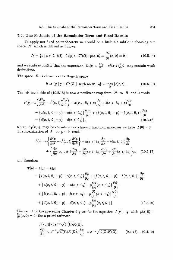
5.3. The Estimate of the Remainder Term and Final Results 253
5.3. T h e E s t i m a t e of t h e R e m a i n d e r T e r m and F ina l R e s u l t s
To apply our fixed point theorem we should be a little bit subtle in choosing our space N which is defined as follows
N - {PIP e C1(~), L2~)] e C~ p(x, O) = Op (x, 0) = 0} (10.5.14)
and we state explicitly tha t the expression L2~] = o_~ _ c 2 . o2p or2 (x, t)-5-~2 may contain weak derivatives.
The space B is chosen as the Banach space
B - {q l q C C~ with norm Ilqll - n~x]q(x,t)l. (10.5.15)
The left-hand side of (10.5.13) is now a nonlinear map from N to B and it reads
02P c 2 F~] =~ -0~ (x, t) O~p ~ 019 OPot - ~x2] + a(x,t, ~tl + P)-~x + b(x,t, ~tl + p)
f
0~1 + {a(x,t, ~tl + p ) - a ( x , t , gl)}-~x + { b ( x , t , ~ t l + p ) - b ( x , t , ul)}0ul0t
+ {d(x,t, ~tl + p ) - d(x,t, ux)}, (10.5.16)
where gl(X, t) may be considered as a known function; moreover we have F[0] = 0. The linearization of F at p = 0 reads
{ 02p _ c2 (x,t) O2p } Op Op Lip] =c ~ ~ + a(x, t, ~q ) -O-xx + b(x, t, ~tl ) Ot
{Oa Ottl Ob(x,t,~tl)O~tl Od } + -~-uu(X,t, f i l ) ~ + ~ -0-/- + -ffuu (x't' Ul) P, (10.5.17)
and therefore
�9 ~] = F ~ ] - Lip]
= {a(x, t, ~1 -Jr p ) -- a(x, t, ~1)} "~X { b ( x , t , ~t I 7 t- p ) - b ( x , t, ?~1)} 0p0t Oa Off1
+ {a(x,t, ~tl + p ) - a ( x , t , U l ) - p - ~ u ( X , t , u l )} Ox
Ob O~q + {b(x,t, tt 1 + p ) - b ( x , t , ?~1)-P-~u(X,t , ?~1)} 0t
Od + {d(x,t, ~t I -~p) -d(x , t , ?~1)-P-ff~u(x,t, ?~1)}. (10.5.18)
Theorem 1 of the preceding Chapter 9 gives for the equation Lip] = q with p(x, O) - ~ 0) = 0 the a priori est imate Ot
Ip(x, t)l < e-�88 v/C(a)K(a),
Op 1 Op c -1 v/C(~)g(gt), (9.4.17) (9.4.19) ]-~x ] < ~- v/C(a)K(gt) , ]-~1 <
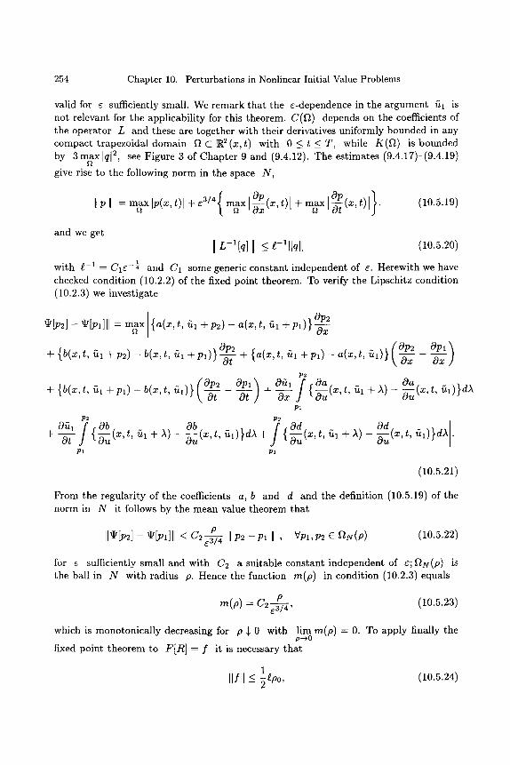
254 Chapter 10. Perturbations in Nonlinear Initial Value Problems
valid for e sufficiently small. We remark that the e-dependence in the argument ?~1 is not relevant for the applicability for this theorem. C(~t) depends on the coefficients of the operator L and these are together with their derivatives uniformly bounded in any compact trapezoidal domain Ft C R 2 (x, t) with 0 <_ t _ T, while K(12) is bounded by 3 m~xlql 2, see Figure 3 of Chapter 9 and (9.4.12). The estimates (9.4.17)-(9.4.19)
give rise to the following norm in the space N,
{ OP(x, t )[+n~x[cOP(x, t ) l} (10.5.19) I P I = II~X [p(x, t) l -4- e 3/4 II~X [-~X -'~ "
and we get [ L-~[q] [ < s I (10.5.20)
1 with l-1 = C le -z and C1 some generic constant independent of e. Herewith we have checked condition (10.2.2) of the fixed point theorem. To verify the Lipschitz condition (10.2.3) we investigate
0p2 ~[p2]- ~[pl][I- m~x {a(x,t , fil + P 2 ) - a ( x , t , fil +Pl )} Ox
+ {b(x, t , 'Ul -'t-/)2) - b(x,t, fil + P l ) } - - ~ + {a(x,t , fil n t- P l ) -- a(x , t , ~ 1 ) } Op2COx Oplox
p2
+ {b(x,t, ~l + p l ) - b ( x , t , gl)} \ --~ Ot +--~x {-~u ' -~u (x' t ' ~l)}dA Pl
P2 P2 -4- ~O U I I { -~ucO b ( x , t , ~t 1 --~- A ) _ cO bou ( x , t , ill)}dA +/{cOd(x,t,-~u ~t l ~t- A ) _ cO d_~u ( X , t, ill) }dA.
Pl Px
(10.5.21)
From the regularity of the coefficients a, b and d and the definition (10.5.19) of the norm in N it follows by the mean value theorem that
P II~[p2]- ~[px]ll < c 2 - ~ I p 2 - pl I , ~pl,p2 e ['~N(P) (10.5.22)
for e sufficiently small and with C2 a suitable constant independent of e; f~N(P) is the ball in N with radius p. Hence the function m(p) in condition (10.2.3) equals
P (10.5.23) re(p) = C2 e3/4~
which is monotonically decreasing for p $ 0 with lim re(p) = O. To apply finally the p-~0
fixed point theorem to FIR] = f it is necessary that
1 Ilfll--_ -~epo, (10.5.24)
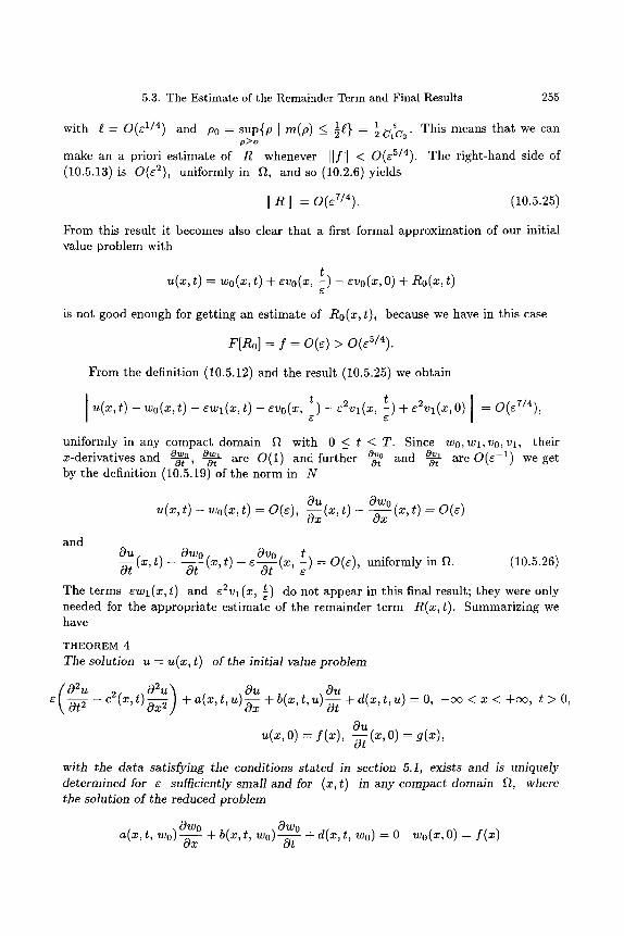
5.3. The Estimate of the Remainder Term and Final Results 255
with g O(E 1/4) and Po sup{p l rn(p) <- ~c;~2" = = l g } = 1 ~ This means that we c a n p>_o
make an a priori estimate of R whenever [[f[[ < O(~5/4). The right-hand side of (10.5.13) is O(~2), uniformly in f~, and so (10.2.6)yields
] R ] = O ( C 7 / 4 ) . ( 1 0 . 5 . 2 5 )
From this result it becomes also clear that a first formal approximation of our initial value problem with
t ~(~, t) = ~o(~, t) + ~o (~ , ; ) - ~o (~ , o) + Ro(~, t)
is not good enough for getting an estimate of R0(x, t), because we have in this case
F [ R o ] = f = O(c) > O(E5/4).
From the definition (10.5.12) and the result (10.5.25) we obtain
t) _~2Vl(X t) 4-~2Vl(X, 0) ] = O(~7/4), U(~, t) -- ~0(X, t) -- ~ (~, t) -- ~0 (~ , ; ,
uniformly in any compact domain ~2 with 0 _ t < T. Since w0, Wl, v0, Vl, their x-derivatives and o~0 o~1 O(1) and further ~ ot o t , ot are Ovo and o.~ a r e O ( e - 1 ) w e g e t by the definition (10.5.19) of the norm in N
and
Ou Owo u(x, t) - Wo(X, t) = 0(~), -~x (X, t) - ~ (x, t) -- 0(~)
Ou Owo Ovo t Ot (x, t) - - - ~ (x, t) - e ~ (x, -)~ - O(c), uniformly in ~. (10.5.26)
t The terms ~Wl (x, t) and E2Vl (x, ~) do not appear in this final result; they were only needed for the appropriate estimate of the remainder term R(x, t). Summarizing we have
T H E O R E M 4 The solution u = u(x, t) of the initial value problem
( 0 2 U _ c 2 ( x t) O2u) Ou Ou c ~ , ~x 2 4 - a ( x , t , U ) O x 4 - b ( x , t , u ) - ~ 4 - d ( x , t , u ) - - O , - c~<x<4-c<~ , t>O,
o~ (~, o) - g(~), ~(~,0)- f(~), ~7
with the data satisfying the conditions stated in section 5.1, exists and is uniquely determined for e sutticiently small and for (x, t) in any compact domain ~, where the solution of the reduced problem
Owo Owo a(x, t, Wo)-~x 4- b(x, t, Wo)--~- 4- d(x, t, wo) = 0 wo(x, O) = f (x)
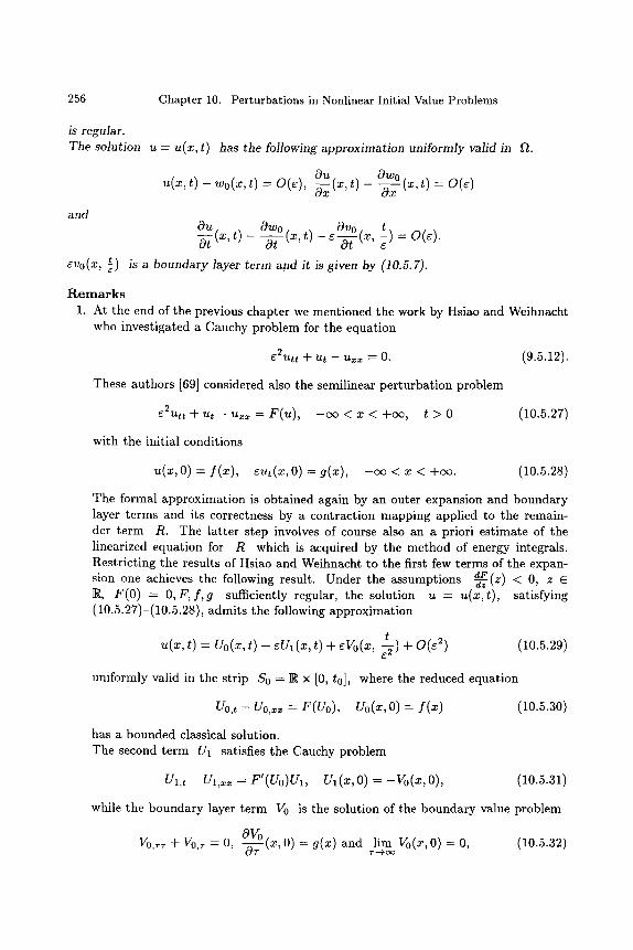
256 Chapter 10. Perturbations in Nonlinear Initial Value Problems
is regular. The solution u = u(x, t) has the following approximation uniformly valid in ft.
and
O~ (~, t) - Owo u(~, t) - ~o (~ , t) = 0 ( ~ ) , ~ --OT (~, t) = 0(~)
Ou OWo Ovo t --or (~' t ) - - -~ (~, t ) - ~ --St- (~' -)~ = o ( ~ ) .
evo(x, t) is a boundary layer term and it is given by (10.5.7).
R e m a r k s 1. At the end of the previous chapter we mentioned the work by Hsiao and Weihnacht
who investigated a Cauchy problem for the equation
"C2Utt -t- Ut -- Uxx = 0. (9.5.12).
These authors [69] considered also the semilinear perturbation problem
e 2 u t t + u t - u ~ = F ( u ) , - o o < x < + o o , t > 0 (10.5.27)
with the initial conditions
u(x, O) = f (x ) , eut(x, O) = g(x), -cx~ < x < +co. (10.5.28)
The formal approximation is obtained again by an outer expansion and boundary layer terms and its correctness by a contraction mapping applied to the remain- der term R. The latter step involves of course also an a priori estimate of the linearized equation for R which is acquired by the method of energy integrals. Restricting the results of Hsiao and Weihnacht to the first few terms of the expan-
dF sion one achieves the following result. Under the assumptions ~-~ (z) < 0, z E R, F(0) = 0, F, f, g sufficiently regular, the solution u = u(x, t), satisfying (10.5.27)-(10.5.28), admits the following approximation
t U(X, t) = Uo(X, t) -Jr ~Vl (x, t) -Jr ~Vo(x, -~ ) Jr- O(~ 2) (10.5.29)
uniformly valid in the strip So = R x [0, to], where the reduced equation
Uo,t - Uo,~ = F(Uo), Uo(x, O ) - f ( x ) (10.5.30)
has a bounded classical solution. The second term U1 satisfies the Cauchy problem
Ul,t - Ul,xx = F'(Uo)U1, UI(X, O) -- - V o ( x , O ) , (10.5.31)
while the boundary layer term Vo is the solution of the boundary value problem
OVo (x, O) = g(x) and lim Vo(x, O) = O, (10.5.32) v0,~- + Vo,- = ~ - ~ r ~
5.3. The Estimate of the Remainder Term and Final Results 257
with T = t / c 2. For details the reader is referred to [69]. A generalization of this result was given by Esham in a Hilbert space setting, [34], [36]. He studied evolution equations of the form
c2utt + ut - A[u] - F(u), (10.5.33)
where A is a positive definite self-adjoint operator.
2. Other nonlinear hyperbolic-parabolic singular perturbat ion problems are reported in [39, 40]. Esham and Weihnacht consider in [39] perturbat ion problems of the form
e 2 u t t + u t - g [ u ] u ~ = f ( x , t ) , t > O , O < x < l . (10.5.34)
where g[u] is the functional
1
0
The initial conditions are
u(x,O) = f (x ) , r = g(x), O < x < 1
and the boundary conditions
u(O, t) = u(1, t) = O, t > O.
An application concerns the oscillations of an extensible elastic string. The same authors consider in [40] the case where g[u] is replaced by some function h(u~). The results are similar as those obtained above in (10.5.29). Other variations on this theme are presented in [35, 38].
3. The modelling of nonlinear waves leads to interesting singular perturbat ion prob- lems. Consider the following initial value problem for a solution of the well-known trans- port equation
o(1 0--t + ~ u 2) = 0 , - c ~ < x < + c ~ , t > 0 (10.5.35)
u(x, O) = Uo(X) (10.5.36)
with -~-oo
f uo(x)dx < oo.
To fix ideas suppose uo(x) > 0 with only one maximum. Because the wave velocity equals u(x, t) the top of the wave will travel faster than the bot tom and so the
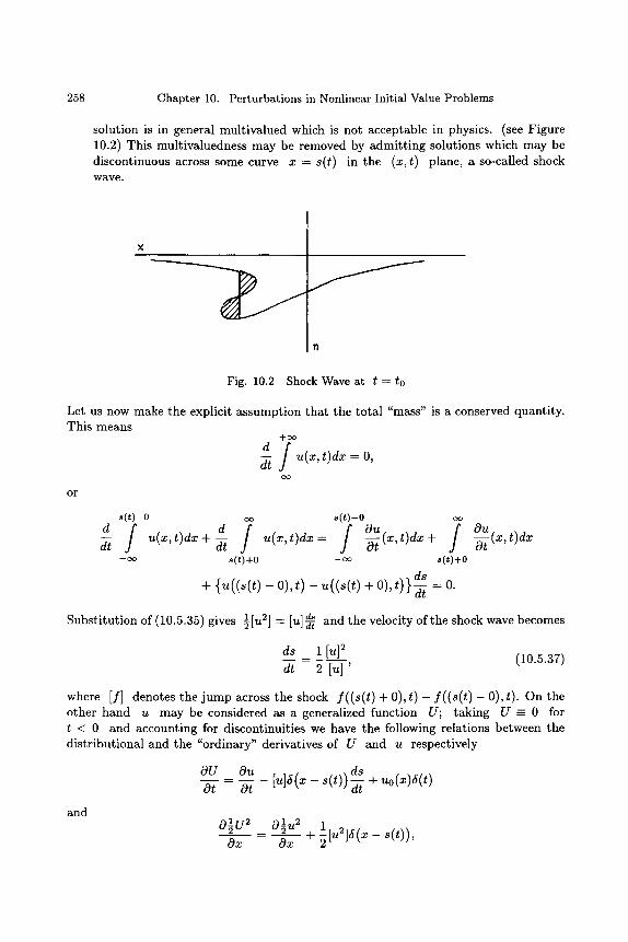
258 Chapter 10. Perturbations in Nonlinear Initial Value Problems
solution is in general mul t ivalued which is not acceptable in physics. (see Figure 10.2) This mult ivaluedness may be removed by admi t t ing solutions which may be discontinuous across some curve x = s(t) in the (x, t) plane, a so-called shock wave.
!
Fig. 10.2 Shock Wave at t = to
Let us now make the explicit a ssumpt ion tha t the to ta l "mass" is a conserved quantity. This means
+ ~
d f u(x,t)dx O, dt
or
s(t)-0 oo ~(t)-0 oo
- f I I I ~ d u(x t)dx + -~d u(x, t)dx - -~Ou (x, t)dx + -~ (x, t)dx dt
-oo ~(t)+0 -oo 8(0+0
ds + { u ( ( s ( t ) - o) , t ) - u ( ( ~ ( t ) + o ) , t ) } ~ = o.
1[u2] --[u] d8 and the velocity of the shock wave becomes Subs t i tu t ion of (10.5.35) gives ~
ds l [u] 2 d-t- = 2 [u] ' (10.5.37)
where [f] denotes the j u m p across the shock f((s(t) + 0), t) - f((s(t) - 0), t). On the other hand u may be considered as a generalized function U; taking U _= 0 for t < 0 and account ing for discontinuit ies we have the following relat ions between the d is t r ibut ional and the "ordinary" derivatives of U and u respectively
OU Ou B
Ot Ot d s
[u]~(~ - ~(t)) ~ + uo(~)~( t )
and 1 2 OsU Ox
lU2 1 _ 0~ + [ u ~ ] ~ ( ~ - ~(t)) - O x -2
5.3. The Estimate of the Remainder Term and Final Results 259
and by (10.5.37) we get for the t ransport equation (10.5.35) together with the initial condition (10.5.36) the equation
Ot + - ~ x U 2) =u0 (x )5 ( t ) , U = O f o r t < O
or because U _-- u except for a set of measure zero
7t-oo
~(x, t) (~, t) + ~ (~, t) 0~ ~ , t > O - - o o
(10.5.38)
valid for any smooth test fucntion ~ with compact support in the region t >_ 0. u = u(x , t) is the discontinuous solution of (10.5.35)-(10.5.36) where the shock cuts off equal areas from the area below and above the curve u = u(x , t), see Figure 10.2. Also this discontinuous solution is not quite satisfactory and therefore one introduces a small dissipation such that u becomes continuous, however, with a steep gradient across the curve x = s(t) . Oleinik [115] considered the singular per turbat ion problem
0u. o--t- + -~x u~ = e Ox 2 , - c o < x < +co, t > O, e > O,
with the initial condition
u~(~, 0) = ~0(~). (10.5.39)
First we remark that this initial value problems is uniquely solvable for all E > 0 and its solution is single valued for e sufficiently small. Therefore the introduction of a gener- alized solution is not necessary; see [147], pp.96-97, where the Cole-Hopf transformation is treated. Oleinik showed tha t u~(x, t) converges for c -+ 0 in distributional sense to a certain function u(x , t) in any interval [a, b] of any straightline t - to > 0 and moreover tha t this function satisfies the relation (10.5.38). Esham [37] took instead of the t ransport equation the Burgers equation
Ou Ou o-~ + u ~ = Z ~ , Z > 0 ,
and he studied the effect of a per turbat ion with a small term ~utt. In particular he investigated the initial boundary value problem
e2 02u Ou 02u Ou - ~ + - - ~ - f l - ~ x 2 + U - ~ - ~ x = f ( x , t ) , - 1 < x < l , 0 < t < T
u(0, t ) = u ( 1 , t ) = 0 , 0 < t < T
Ou u(x,O) = g(x) , ~ - h(x) , O < x < l.
The limit with ~ --+ 0 gives a transit ion from a hyperbolic to a parabolic differential equation. Finally we mention the work by Lax and Levermore [93]; they added to the
260 Chapter 10. Perturbations in Nonlinear Initial Value Problems
equat ion (10.5.35) a small d i spers ion t e rm and they considered the singular per tu rba t ion problem
072 072 0372 0--~ + u -~x - e O x 3 ' - co < x < + co , t > O ,
with the initial condit ion
~(~ , 0 ) = ~0 (~ ) , - ~ < �9 < + ~ .
This differential equat ion is the well-known Korteweg-de Vries equation; it describes long-waves in relatively shallow canals.
Exercises
1. Give a first order approximat ion of the solution of the system
du dv = v, e--rr = -t-u n - v , n = 2 , 3 , . . . , t > O,
dt
with ~(0) = ~ > 0, ~(0) = ~.
Specify the t-interval where the approximat ion is valid.
2. Investigate the initial value problem
d2u (du) 2n+1 ~-gi ~ + -gi
- e ~ = 0 , n = 0 , 1 , 2 , . . . , t > 0 ,
with du
~(o) = ~, 7 i ( o ) = ~.
3. Determine a first order approximat ion of the solutions, including their first order derivatives, satisfying the initial value problems
i. e { 02~ - c2(x t) 02~ o~ , ~ } + - ~ + s i n u - - O , - c o < x < + o o , t > O o~ (~, 0 ) = g (~ ) - ~ < �9 < + ~ . u ( x , 0) -- lr sin x, ~
ii. e{ -O-iV o2'` - c2 ( x , t ) ~ } + -o-~~ - sin u = O, - o o < x < +co, t > O, Ou u ( x , O ) = s inx, -bT(X, 0) = g ( x ) , -cx~ < x < +co. where g ( x ) is an
arbi t rary C~176 Sketch the solution w ( x , t) of the reduced initial value problem for the values t = 0 , t = t l > 0 and t = t 2 > > t l (seeRef. [83]).
Chapter 11
S I N G U L A R P E R T U R B A T I O N S IN N O N L I N E A R B O U N D A R Y V A L U E P R O B L E M S
OF S E C O N D O R D E R
1. I n t r o d u c t i o n
In this chapter we turn our attention to singular perturbations in nonlinear bound- ary value problems of second order. As in the preceding chapters 7 and 8 we first construct a formal solution consisting of a combination of an approximation of the so- lution of the unperturbed problem with ~ = 0 and a correction due to the loss of a boundary condition. As to the proof of the justification of this procedure we investigate again the error in the formal approximation and show that this error becomes small when the perturbation parameter goes to zero. We treat nonlinear ordinary differential equations and also partial differential equations of elliptic type, the latter less extensive than the former because of complex and tedious calculations. In section 2 we discuss the boundary value problem
d2u du ~-d--~ + a(~ ~) + b(~ u) - o, ' ~ ' o < x < l , u (O)- -a , u(1)--/3, (11.1.1)
with a(x,w)=fiO for 0<_x_<l and all values of wEIR. We get a boundary layer at x = 0 whenever a ( x , w ) > a o > O and one a t x - 1 whenever a(x, w) < a0 < 0. The justification of the construction is established by using again the fixed point theorem of section 10.2; it will appear that the verification of the condition 10.2.2 requires some extra effort. In the next section 3 we drop the condition a(x, w) -71= 0 and this may give rise to the occurrence of interior layers (shocks). The theory is illustrated with the well-known Lagerstrom-Cole example
d2u du ~-ff-~x2 + U--~x u = O, u ( 0 ) = a < 0 , u ( 1 ) = 1 3 > 0
for the cases / 3 > a § and f l < a + l . Another interesting example is the boundary value problem
d2u du e~x2 +U~x x = 0 , u ( - 1 ) = a , u(+l ) - / 3
262 Chapter 11. Perturbations in Nonlinear Boundary Value Problems
for several values of a and ft. This example shows the "capriciousness" of singular perturbations, a phrase from W. Wasow [144]. Section 4 is devoted to autonomous conservative equations of the type
~2 d2 u + f (u) = O, u(O) - a, u(1) = ~,
and we use phase-plane representation and some geometric intuition. In section 5 we present the theory of Haber and Levinson [59] concerning the more general boundary value problem
d~ ( d ~ ) ~-~2 = / u , ~ , u(0) = a and u(1) = ~,
where .f(u, v) is submitted to the condition
0/( dg ) Ov g ( ~ ) ' ~ ( ~ ) >0, 0 _ _ _ x < ~ a n d ~ h(x),-~x(X) < 0 , 5 :<x_~ 1,
where g and h are solutions of the reduced equation ( r with g ( 0 ) = a , h ( 1 ) - and g(&) = h(&). The theory is rather technical and therefore we do not give the
proof of the asymptotic approximation of the solution, but the result will appear to be very plausible by the experience already obtained in the preceding sections. Finally, we treat in the last two sections the elliptic boundary value problem
02u 02u ~ Ou -c ~ + -~y2 ] + a(x, y)-~y + b(x, y; u) -- 0, (11.1.2)
where (x,y) belongs to a bounded domain ff and u(x,y) satisfies a boundary condition along the boundary Off.
Ob(x, u) < 0 for all (x,y) e f and The analysis is facilitated by the assumption ~ y, all u E ]~; the reason is that this requirement is sufficient for the application of a generalization of the maximum principle or the fixed point theorem necessary for the approximation of the remainder term.
The general problem with the equation
( 02u 02u ) Ou Ou c \ cOx2 + ~ + a(x, y, u ) ~ W b(x, y, u)-~y + c(x, y, u) -- O, (~, y) e ~ (11.1.3)
involves many complications as may be inferred already from the theory of section 2 where the boundary value problem (11.1.1) has been discussed. Moreover the behaviour of the solution in the neighbourhood of the extremal points of Off where the subcharacteristics are tangent to 0fl is another source of very unattractive calculations, see Chapter 8, section 3; the interested reader is referred to [53, 62, 63, 78].
2.1. The Formal Approximation 263
2. B o u n d a r y Value P r o b l e m s for Q u a s i l i n e a r O r d i n a r y Di f fe ren t i a l E q u a - t ions
2.1. T h e F o r m a l A p p r o x i m a t i o n
As mentioned in the introduction we start with singularly perturbed boundary value problems for ordinary quasilinear differential equations. So we discuss the following boundary value problem
d2u du 6-~x 2 Jr- a(x, u) ~x -q- b(x, u) = O, 0 < x < 1, (11.2.1)
with the boundary conditions
u(O) = c~, u(1) =/3. (11.2.2)
The parameter e is small positive and further we make the following assumptions i. a ( x , u ) _ a0 > 0 for all values of x E [0, 1] and for all values of u E IR. This
condition may be replaced by a(x, u) < a0 < 0 and the following development may be carried out in a similar way. This requirement is introduced to prevent a singularity in the reduced equation and the occurrence of interior layers (see section 7.9,.6)
ii. the solution of the reduced boundary value problem
a(x, w) dw -~x + b(x' w) = O' O < x < l, w(1) -- ~, (11.2.3)
is uniquely determined and differentiable in the segment [0, 1]. iii. To avoid tedious bookkeeping we assume for convenience that the coefficients a(x, u)
and b(x, u) are infinitely often differentiable with respect to x and u. It follows from the assumption above that the solution w(x) of (11.2.3) is also a C ~- function in [0, 1]. The choice of the boundary value w(1) - /3 is in accordance with the condition a(x, u) > a0 > 0, see (7.2.12)-(7.2.14).
The formal approximation is constructed again with the aid of a composite expan- sion
N N + I
Z Z + (11.2.4) c
k = 0 k = 0
To obtain an estimate of RN(X;---c) which is uniformly small in [0, 1] it will appear that it is sufficient to take N = 1. The function To(X) is defined by the unique solution of the reduced problem (11.2.3) and the function Wl(X) satisfies the equation
( dwo ) e --d-~x 2 + d x 2 + . . . + a ( x , w o + e W l + . . . ) -~x + e --d--xx + " "
+ b(z, w0 + 6Wl + ' " ) = 0,
264 Chapter 11. Perturbations in Nonlinear Boundary Value Problems
or in a first approximation
dwo dwl {a(x, Wo + ewl) - a(x, w0)}--~- x + ea(x, wo) dx
d2wo . -~{b(x, w 0 --~ ~ W l ) - b(x , Wo) } - - c d x 2
or with the aid of the mean value theorem
d w l { O a d w o O b } d2wo (11.2.5) a(x, wo)--~ x + ~u(X, w o ) ~ + ~u(X, wo) wl = dx 2 ,
valid for 0 < x < 1, while the boundary condition is
w1(1) = 0 .
We remark that" this boundary value problem for Wl and generally all the boundary value problems for the terms wk of the so-called outer expansion are linear, so that no complications in the construction of the outer expansion arise. To meet the boundary condition w(O) - a we should introduce the boundary layer terms ~kvk(~c ) with ~ - - ~ . Putt ing
u(~) ~ ~ k ~ k ( ~ ) + ~k~k(~)"= W + Y
and assuming that the outer expansion W is known we get for the boundary layer part V the differential equation
d2W l d2V ( dW l dV ) ~--s + - - ~ + a(x, W + Y) ~ + -~ 7 ( + b(x, W + Y) = O,
o r
1 2V1 { } d~ 2 ~- a(x, W + v) dV dW - ~ - + a(x, W + V)-~x + b(x, W + V) = -~ ,
o r
dzV dV dW -+- a(x, W + V) ~ + 6{a(x, W + V) - a(x, W)}-~x + r W + V) - b(x, W)} d~ 2
( d2W dW "1 = - r + a(x, W) ~ + b(x, W) ~ := d(x,r (11.2.6)
In case we take N = 1 we have d(x, r - O(r uniformly in [0, 1]. We write this equation as follows
d2vk ~r _~_ + a{e~, ~r (wk(r vk(~)}~r kdvk d~
dwk + ~[a{~, r ~ ( ~ (~) + ,~(~))} - a{~, r ~ ~ ( ~ ) } ] r ~ - ~ (~r
+ ~[b{~, ~ ( ~ ( ~ ) + ~(~))} - b{~r ~ ~ ( ~ ) } ] = d(~, ~).
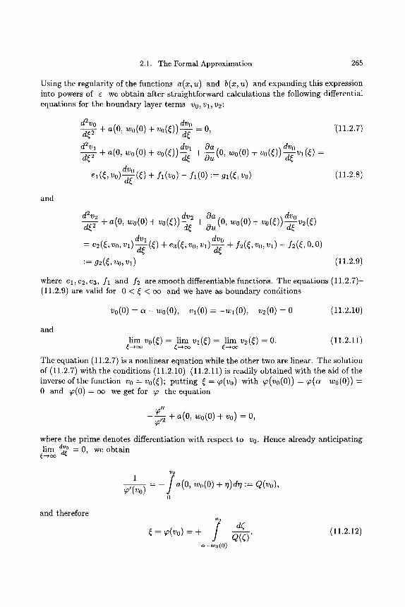
2.1. The Formal Approximation 265
Using the regularity of the functions a(z, u) and b(x, u) and expanding this expression into powers of e we obtain after straightforward calculations the following differential equations for the boundary layer terms v0, vl, v2"
d2vo dvo d~C------- Z 4. a (0, wo(O)+ vo(~))-~__ = O, "(11.2.7)
d2Vld~ ----~ dVl -~uOa (0, w0(0) + v0(~)) dvo + a(O, wo(O) + vo(~r - -~ 4- -d-~Vl (~r =
dvo el(~, V o ) T ( ~ ) 4. fl(vo) -- fl(O)"-- gl(~, Vo) (11.2.8) a ;
and
d2v2 Oa (0, wo(O) + vo(~C)) dvo
d~--- 7 4. a(0, w0(0) + v0(~)) ~ + Ouu -d-~ v2(~)
dvl dvo ~- e2(~, VO, V l ) - ~ ( ~ ) + e3(~, VO, V l ) ' - ~ 4. f2(~ , VO, Vl) -- f2(~ , O, O)
, J
:= g2(~, vo, ~l) (11.2.9)
where el, e2, e3, fl and f2 are smooth differentiable functions. The equations (11.2.7)- (11.2.9) are valid for 0 < ~ < c~ and we have as boundary conditions
Vo(O ) -- OL -- Wo(O), Vl(O) -- - -Wl(O) , v2(O ) -- 0 (11.2.10)
and lim Vo(~)- lim v~(~)- lim v2(~)= O. (11.2.11)
The equation (11.2.7) is a nonlinear equation while the other two are linear. The solution of (11.2.7) with the conditions (11.2.10)-(11.2.11) is readily obtained with the aid of the inverse of the function v 0 - v0(~); putting ~ = ~ (v0 )wi th ~ ( v 0 ( 0 ) ) - ~ ( a - w 0 ( 0 ) ) - 0 and ~(0) - c~ we get for ~ the equation
- - - + a(O, ~ o ( 0 ) + ~o) = O,
where the prime denotes differentiation with respect to v0. Hence already anticipating lim ~ = 0, we obtain ~--+ cx~ d~
vo
1 _ - - / a(O, wo(O) + r/)dr/:= Q(vo), ~'(~o)
0
and therefore Vo
~ - v(~o) - + / a-wo(O)
de Q(~)" (11.2.12)
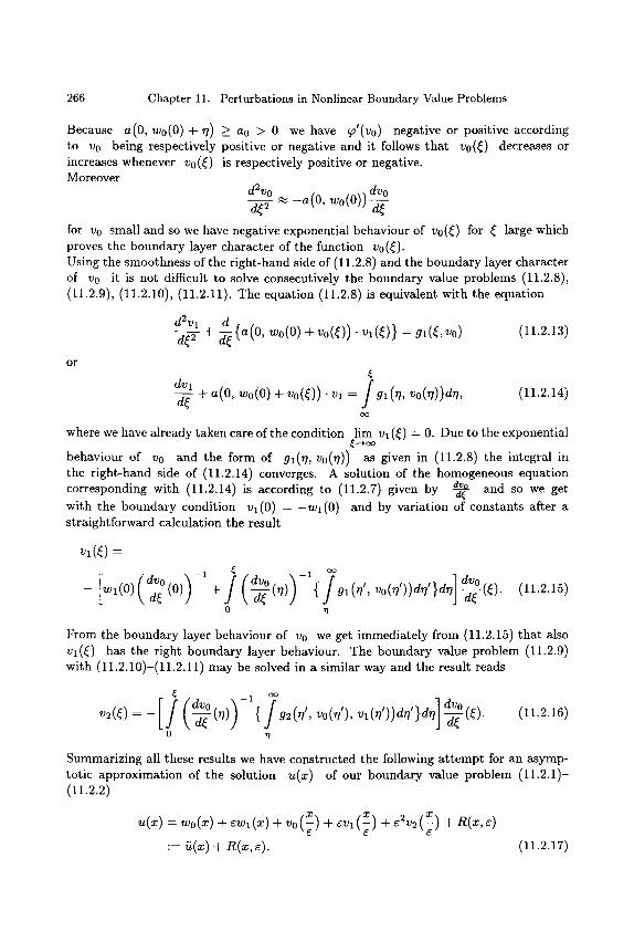
266 Chapter 11. Perturbations in Nonlinear Boundary Value Problems
Because a(0, w0(0)+ y) > a0 > 0 we have ~'(v0) negative or positive according to v0 being respectively positive or negative and it follows that v0(~) decreases or increases whenever v0(~ c) is respectively positive or negative. Moreover
dvo ~ 0 (0, w0(0)) d~ 2 ~ - a
for v0 small and so we have negative exponential behaviour of v0(~) for ~r large which proves the boundary layer character of the function v0(~r Using the smoothness of the right-hand side of (11.2.8) and the boundary layer character of vo it is not difficult to solve consecutively the boundary value problems (11.2.8), (11.2.9), (11.2.10), (11.2.11). The equation (11.2.8) is equivalent with the equation
d2Vld~--- ~- -I- ~d { a (0, wo(O) + vo(~)) �9 Vl (~) } = gl(~, Vo) (11.2.13)
o r
dvl / d----( + a(0, w0(0) + v 0 ( ~ ) ) �9 V l - - gl (r/, v0(r/))dr/, (11.2.14)
oo
where we have already taken care of the condition lim Vl (~) = 0. Due to the exponential
behaviour of v0 and the form of gl(r/, v0(r/)) as given in (11.2.8) the integral in the right-hand side of (11.2.14) converges. A solution of the homogeneous equation corresponding with (11.2.14) is according to (11.2.7) given by d,o and so we get d~ with the boundary condition Vl(0) = -Wl (0) and by variation of constants after a straightforward calculation the result
v~(() -
[ - - W 1 (0) ~, d~ (0) + \ d~ (7"1) { f gl 07', vo(rl/))drl/}drl o
dvo --~-(~r (11.2.15)
From the boundary layer behaviour of v0 we get immediately from (11.2.15) that also vl(~) has the right boundary layer behaviour. The boundary value problem (11.2.9) with (11.2.10)-(11.2.11) may be solved in a similar way and the result reads
) / v~(~) = - - ~ ( ~ ) { g~(~', v0(~'), v~(~'))a~'}e~ -~-(~1. o ~?
(11.2.16)
Summarizing all these results we have constructed the following at tempt for an asymp- totic approximation of the solution u(x) of our boundary value problem (11.2.1)- (11.2.2)
G
:= ~(~1 + R(~, ~1. (11.2.17)
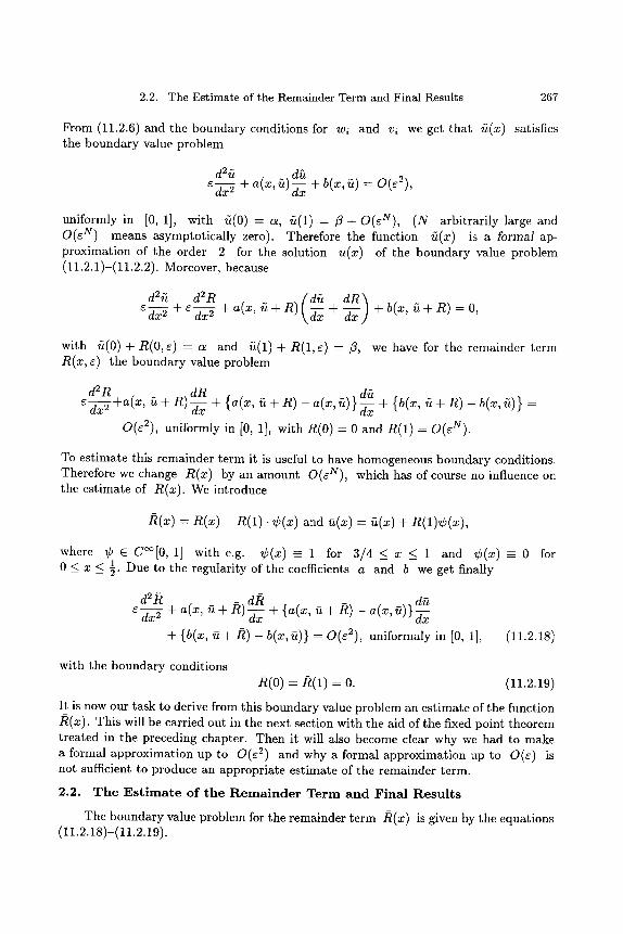
2.2. The Estimate of the Remainder Term and Final Results 267
From (11.2.6) and the boundary conditions for w~ and v~ we get that ~(x) satisfies the boundary value problem
d2u dfi e--~x 2 + a(x, ft) + b(x ~) = O(e 2)
uniformly in [0, 1], with ~(0) = c~, ~(1) = ~ + o(eN) , (N arbitrarily large and O(e N) means asymptotically zero). Therefore the function g(x) is a formal ap- proximation of the order 2 for the solution u(x) of the boundary value problem (11.2.1)-(11.2.2). Moreover, because
d 2 t t d 2 R ( d f t d R ) r 2 + r 2 + a(x, fi + R ) ~x + ~ + b (x, g + R ) - O,
with g ( 0 ) + R(0, e) - c~ and f i (1)+ R(1, e) = ~, we have for the remainder term R(x, e) the boundary value problem
d2R . dR d~ e ~ + a ( x , ft + R ) ~ + {a(x, ft + R) - a(x, ft) }--~x + {b(x, ft + R) - b(x, ~) } -
O(e2), uniformly in [0, 1], with R(0) - 0 and R(1) - o(eN).
To estimate this remainder term it is useful to have homogeneous boundary conditions. Therefore we change R(x) by an amount o(eN), which has of course no influence on the estimate of R(x). We introduce
R(x) - R ( x ) - R(1) . r and ~(x) = g ( x ) + R(1)r
where r C C~[0, 1] with e.g. r - 1 for 3/4 _< x _< 1 and r - 0 for 1 0 _< x _< 5" Due to the regularity of the coefficients a and b we get finally
d2R d/~ d~ c--~x 2 + a(x, ~t + R) -~x + {a(x, ~ + [~) - a(x, u)} d---x
+ {b(x, ~ + it) - b(x, ~)} = O(e2), uniformaly in [0, 1], (11.2.18)
with the boundary conditions R(0) = R(1) = 0. (11.2.19)
It is now our task to derive from this boundary value problem an estimate of the function /~(x). This will be carried out in the next section with the aid of the fixed point theorem treated in the preceding chapter. Then it will also become clear why we had to make a formal approximation up to O(~ 2) and why a formal approximation up to O(e) is not sufficient to produce an appropriate estimate of the remainder term.
2.2. T h e E s t i m a t e of t h e R e m a i n d e r T e r m a n d F ina l R e s u l t s
The boundary value problem for the remainder term /~(x) is given by the equations (11.2.18)-(11.2.19).
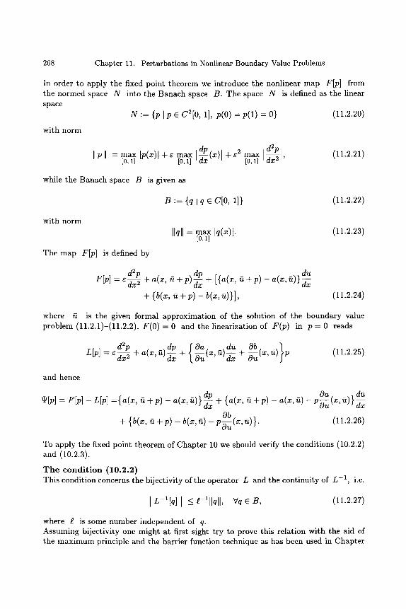
268 Chapter 11. Perturbations in Nonlinear Boundary Value Problems
In order to apply the fixed point theorem we introduce the nonlinear map F~] from the normed space N into the Banach space B. The space N is defined as the linear space
N := { P I P e C2[0, 1], p(O) = p(1) = O} (11.2.20)
with norm
I pl - max Ip(x)l + ~ max I dp e 2 d2p to,~ tO, l~ ~(~)1 + ~O,al:~ I~1, (11.2.21)
while the Banach space B is given as
B := { q l q e C[0, 1]} (11.2.22)
with norm
The map F[p] is defined by
Ilqll = max Iq(x)l. (11.2.23) [0,1]
d2p dp d~ F[p] - e--~x 2 + a(x, fL + P)-~x + [{a(x, fL + p) -- a(x, u)}~xx
+ {b(~, ~ + p) - b(~, ~)}], (11.2.24)
where fi is the given formal approximation of the solution of the boundary value problem (11.2.1)-(11.2.2). F ( 0 ) = 0 and the linearization of F(p) in p = 0 reads
d2p dp { Oa dfz Ob } Lip] - e --~-~x 2 + a ( x , u) -~x + ~ ( x , ~ ) -~x + ~ ( x , ~ ) p (11.2.25)
and hence
dp {a(x ~ p) a(x, ~) Oa (x, fL) } d~ q2[p] = F[p] - LiP] - { a(x, fi + p) - a(x, fi) } ~x + ' + - - P--~u dx
Ob (x, fi)} (11.2.26) + {b(~, ~ + p) - b(~, ~1 - p ~
To apply the fixed point theorem of Chapter 10 we should verify the conditions (10.2.2) and (10.2.3).
The condit ion (10.2.2) This condition concerns the bijectivity of the operator L and the continuity of L - I , i.e.
] L-l[q] ] < l-lllqll, Vq E B, (11.2.27)
where I is some number independent of q. Assuming bijectivity one might at first sight try to prove this relation with the aid of the maximum principle and the barrier function technique as has been used in Chapter
2.2. The Estimate of the Remainder Term and Final Results 269
7, subsections 7.2.3 and 7.2.5. However we meet here a rather unpleasant situation since for the application of the maximum principle we should require
Oa dfi Ob --a~ (~' ~) " ~ + ~u (~' ~) < ~ < o (11.2.28)
Because ~da = O(1) in the neighbourhood of x = 0 and because we did not fix the sign of oa (x, ~) in this neighbourhood we are not sure that we can fulfil this condition. The trick to introduce i5 = pe -~ does not help either since in that case t5 satisfies the equation
d2i~ 2sO} di6 L[~] =e-~x2 + {a(x, ~t) + --~x +
[ Oa d~t Ob ] ~02 + ~a(x, ~t) + { -~u (X, {t) -~x + Ou (x, Ct) } ~ = e -ox �9 q(x).
Due to the regularity of a(x,~), b(x,~), a(x, fi) > a0 > 0 and the boundary layer behaviour of ~ there exist positive constants A,B, C and K, independent of e, such that
Oa Ob d~t K 0 < a(x,~z) <_ A, uu'[--ff-(x'u)l < B, 'au-[-z-(x'~)[ < C and [~x[ < - - .
Therefore z9 must satisfy
( evq2q-vqA+ A - C = V~0q-~- -~ ---~-c A - - - - 4 - C < 6 < 0 C E '
but this is not possible without restrictions on A, B and K. The remedy to overcome the difficulty in (11.2.28) has been given by A. van Harten [62]. He proved the following lemmas.
LEMMA 1 Let M be the differential operator
d 2 d M := c~(x) d---~x2 + ~(X)~xx + 7(x),
with ~, # ~ d ~ ~o~ti~uou~ ~nd ~(~) > ~0 > 0, W e [0, 1]. If t h ~ ~i~t~ ~ f ,~ctio~ X E C2[0, 1] and positive constants io, 51, 52 such that
O < 51< X(x) < 52, M[X] < - io < O, V x E [ 0 , 1 ] (11.2.29)
then the solution of the boundary value problem
M [ p ] - q , p ( O ) - p ( 1 ) = O ,
where q E C[0, 1] satisfies the estimate
m a x Ip(x)l < 52eO 1 max Iq(x)l. [ 0 , 1 ] - - [ 0 , 1 ]
(11.2.30)
270 Chapter 11. Perturbations in Nonlinear Boundary Value Problems
P r o o f The function r = x- lp satisfies the equation M[rx] = q or
d2r { dx }dr /l:/[r] := a ( x ) x ( x ) ~ + 2a(x) (x) + ~(x)x(x) + M[x]r(x) = q(x).
Since M(X) is negative we may apply the barrier function technique for es t imat ing r. We take as barrier functions the constant ~o 1 max Iq(x)l and we get immediately
[0,1]
J~r [~01 m a x Iql] < - m a x Iql < I/1~/[r(x)] I < + m a x Iq[ < -~7 / [ - l o 1 max [q[]" [0,1] . . . .
Hence we obtain by the fundamental lemma of subsection 7.2.2
[r(x)l < lo 1 max [q(x)[, Vx e [0, 1], - [o, ll
or
]p(x)l < ~olX(x) max [q(x)l < ~o~52 max Iq(x)l, [0,1] - [0,11
Vx E [0, 1].
We remark tha t this es t imate guarantees the uniqueness of the solution of M[p] - q; (see also e.g. [89]).
LEMMA 2
Let L be the differential operator as given in (11.2.25) then there exists a function X(X) satisfying the conditions of LEMMA 1, i.e. )(.(X) E C2[0, 1] and there exist positive constants 51 and 52 independent of r such that
L[X]=-I+O(r O < x < 1 (11.2.31)
with 0 < 51 < X < 52- (11.2.32)
P r o o f The function X is constructed as the first order approximation of the solution of the boundary value problem
L[X] = - 1 with x(O) = ko and X(1) = k l ,
where the constants k0 and kl are chosen such tha t (11.2.32) holds. The function X has the familiar form
with (I)0 the outer solution and ~0, ~1 the boundary layer terms. For details of the proof the reader is referred to [62].
2.2. The Estimate of the Remainder Term and Final Results 271
COROLLARY Combining both lemmas we obtain from Lip] = q, p(O) = p(1) = 0 the a priori estimate
max Ip(x)l < go~52 max Iq(x)l, (11.2.33) [o, 1] - [0,1]
1 with 62 and go independent of c; take for instance go = ~-
To proof finally (11.2.27) we need also a priori est imates of dd~(x) and d-~(X);dx2 these estimates can easily be made by using the differential equation L~v] = q and the interpolation theorem tha t has been used in section 7.2.5, Remark 6. We write L ~ v ] = q as
d2p dp L[p] = e~-~x 2 + A(X)~xx + #(x)p = q,
with Oa d~z Ob
A(x) = a(x, ~) and #(x) = ~u(X, u) dxx + Ou (x, ~).
From Lip] = q we have
max I d2P[0,1] ~-1{ /~071~ ~071~ dp I~o,31~ I~o,31~ } ~x21-< Iq' + [AI" ~0,al~ I~xl + '#] IP] �9 (11.2.34)
From the interpolation theorem follows the existence of positive constants c and d such that
m~x I dp ~ P (~) [0,1] -d--xx ( x ) l < c r~o ?~ ] I --~x 2 I+ d c - l r~o ?l ~ Ip(x)l, (11.2.35)
where c may be any positive number and d depends on]y on the interval of x-values, see section 7.2.5, Remark 6.
1 we get with d independent of e. Taking c - ~r max IA(x)l} -1 [0,1]
e-1 max I,~(~)1 max I dp 1 d2p ~o,31~ Ip(~)l [0,1] [0,1] ~(~)l < ~ ~07~ I~(~)1 + 2d~-~{ ~07~ 1~(~)1}2
and subst i tut ion into (11.2.34) gives
[0,1] ~X 21 -~ 2e- ~O,alfflq(x)[ + 2e 2de { ~O,al~[A(x)l + ~O,al~:[#(x)[ ~o,al~[p(x)[.
Using now (11.2.33), max I~(~)1 - o(1) , max I,~(~)1 - o(1) we obtain finally the [0,1] [0,1] results
max I d2p [0,1] ~X 2(x) I ~ C2c-2~o?1~ Iq(x)l, (11.2.36)
and with the aid of (11.2.35)
m~x I dp ~-1 ~x(X) I _~ C1 ~o71~ Iq(x)l, (11.2.37) [o, 1]
272 Chapter 11. Perturbations in Nonlinear Boundary Value Problems
where C1 and C2 are constants independent of e. Hence (11.2.33), (11.2.36) and (11.2.37) yields the required estimate
[L-l[q] [ = ] p [ = m a x [ p ( x ) l + e m a x I dp r d2p
Eo, j Eo, j §
< e-lllqll, Vq e B (11.2.27)
with 1-1 independent of e. We proceed now to the second condition (10.2.3) of the fixed point theorem.
T h e c o n d i t i o n (10.2.3) To check this condition we investigate
I]~(P2)- ~(pl)[[ ~ max [0,1]
-[- max [0,1]
-~- max [0,1]
-~- max [0,1]
max [o, 1]
-t- max [o,~]
dp2 { a ( x , ~t + p2) -- a ( x , ~t + pl)}--~x [
{a(x, fi + P l ) - a ( x , fi)} dx dx [
Oa d~t {a(x, ~t + P 2 ) - a ( x , ~t + P l ) - ( P 2 - Pl)~u(X, U-~- Pl)}~XX I
Oa Oa d~t (P2 - -P l ){ ~UU (X, '~) -- ~U (X, U "[" Pl) } dxx [
Ob {b(x, ft - I - p2 ) -b (x , ft - [ - P l ) - (P2-PI)}o--~( x, 'u +P l ) [
Ob (x, ~) - Ob
We consider two elements pl and p2 in the ball ~N(P) with radius p _ 1 and we get on account of the regularity of the coefficients a(x, u) and b(x, u), the formal approximation fi (11.2.17) and the definition of the norm (11.2.21) the result
IIIII(p2)- ~I/(pl)II--~ c c - l P I P 2 - Pl I , 'v'p e aN(p) , p ~ 1, (11.2.38)
where C is a constant independent of e, and it follows that condition (10.2.3) holds.
Now we are finally in the position to apply the fixed point theorem to the boundary value problem (11.2.18)-(11.2.19) for the remainder R. The function re(p), see (10.2.3), is the monotonic function C e - l p and the number P0 (10.2.4) becomes
p 0 = s u p { p [ 0 _ P _ < 1, c e - l p < ~.} = 2C"
Because the right-hand side of (11.2.18) is O(e2), uniformly in [0, 1] we can satisfy the condition
I l f l - - O(~2) < ~ p o -- 4C '
3. Transition Layers 273
for e sufficiently small; so we get by (10.2.6) the result that /~ exists with
I R I ~ 2g-~ Ifll = o(~2) �9 (11.2.39)
Moreover the solution /~ is also unique since /~ lies clearly in the domain L- l [ f tB (gPo) ] - L-1 [gts( st2~] (see proof of fixed point theorem) ge]J From this we obtain also the result that the original boundary value problem (11.2.1)- (11.2.2) has a unique solution for e sufficiently small. Summarizing we have the following theorem.
THEOREM 1 Be given the boundary value problem
d2u du ~a-fi~ + ~(~' u) ~ + b(~, ~) = o, 0 < x < 1 (11.2.40)
with the boundary conditions
u(O) -- a, u(1) -- ft. (11.2.41)
The coefficients a and b are of class C~([0, 1], ]R) with a(x, u) >__ ao > O, Vx E [0, 1], Vu C 1R and with ao some positive constant. Under the assumption that the solution of the reduced boundary value problem
a(x, w) dw --dTx + b(x, w) - O, - 0 < x < l, w ( 1 ) = / ~
exists uniquely in [0, 1] we have the result that also the solution of (11.2.40)-(11.2.41) exists uniquely for e sutticiently small. Moreover the following approximations hold, uniformly in [0, 1],
Ue(X) -- WO(X)+ CWl(X)-~- VO(x) + gVl (X) "~- 0(C2 ) (11.2.42)
and du~ d~o ~ ~ ) + 0 ( ~ ) d~ (~) = ~ + ~~ "
(11.2.43)
The outer solution terms Wo and 6W 1 a r e given by (11.2.3) and (11.2.5) and the boundary layer terms vo and CV 1 by (11.2.12) and (11.2.15).
3. Transit ion Layers
We consider again the boundary value problem
d2u du r 2 + a(x, u) -~x + b(x, u) = 0, 0 < x < 1, (11.3.1)
with the boundary conditions
274 Chapter 11. Perturbations in Nonlinear Boundary Value Problems
u(0) - a, u(1) =/3 . (11.3.2)
In contrast with the preceding section we drop the conditions (i) and (ii) of subsection 11.2.1. This means tha t a(x, u) may become zero for some value of u and x with 0 < x < 1 and there is the risk tha t the reduced equation
a(x, w) dw + b(x, w) = O, (11.3.3)
becomes singular; take e.g. a(x, u) = u and aft < O. In this case we are in a si tuation similar as tha t of a turning point, discussed in section 7.3, with the difference tha t this point is not a priori given by some value of x, but its location depends in general on the differential equation and the boundary values. Instead of the conditions i) and ii) we suppose now tha t there exist functions UL (x) and uR(x) which satisfy the requirements
duL a (x , UL ) ~ n t- b(x, UL ) = O,
duR a(x, u R ) - ~ + b(x, uR) = O,
O < x < &, uL(O) =c~ and (11.3.4)
_< x < 1, uR(1) -- fl, (11.3.5)
while a(x , UL) < O, 0 < X < ~ and a(x, uR) > 0, ~ < x < 1. (11.3.6)
Assuming tha t our boundary value problem has a solution we may infer from Theorem 2 of section 10.3 tha t UL(X) and uR(x) are good approximations of u(x) up to O(e) in the intervals 0 < x < ~ and ~ < x < _ 1 respectively.
du We remark tha t according to this theorem the values of ~-~x (x) in x - 0 and x - 1 are of no relevance in an O(E)-approximation of u(x). In the supposit ion tha t UL(X) and uR(x) are known we have now to construct an interior layer connecting u ,.~ UL(X) and u ~ uR(x); it will appear tha t this layer has the appearance of a shock wave whenever UL(5:) =/= uR(~). This transi t ion is analyzed by stretching the x-variable around the still unknown value of ~ by
x - ~ -- ~ , (11.3.7)
and we represent the transition layer by a function v(~) that should satisfy in approx- imation the relation
U(X) ,~ UL(X ) n t- V(~) -- UL(X) + V E
with lim v(~) = 0 and lim v(~) = uR(~ + 0) - UL(X, -~- 0). (11.3.9)
~-~-~ ~ + o o
The la t ter limits implies tha t the solution UL(X) of (11.3.3) can be continued into an interval 0 < x < ~ + (f, where 6 is arbitrari ly small positive but independent of e.
3. Transition Layers 275
Substi tut ion of (11.3.8)into (11.3.1) gives
r d2v ) + - ~ + ca(g: + ~-~, U L "+" V)~ dui 1 dv \ dx +-e-~ +r
dv - d=~ ~ a (~ + ~ , ~ ( ~ + ~ ) + ~ ( ~ ) ) - ~
duL (~c + e{) + 6{a(& + r UL(X + c~) + v({)) -- a(5; + r UL(X + r
+ ~{b(~ + ~, u~(~ + ~) + ~(~)) - ~(~ + ~, u~(~ + ~)} = 0.
Assuming sufficient regularity of the functions a and b we get in first approximation the following boundary value problem for v(~)"
d2v dv d{------ 5 + a(~, UL(5:) + v)--~ = O, (11.3.10)
with
lim v({) = 0 and lim v({) = UR(~C) -- UL(g:). ~-+-c~ ~ + m
Integrat ion of (11.3.10) with lim dv 7~(~) = 0 yields {-+-m
(11.3.11)
dv f dv d~ c + a(~, UL('X) + v(~')) ~-~(~')d~' = O, - - ( 2 0
o r
uL(~)+v
d---~ + a(~:, rl)drl = O, with lim v(() - UR(~:) -- UL(~:). (11.3.12) ( ~ + ~ ,,L (i:)
In case uR(~:) > UL(~:) the function v(() is monotonically increasing from zero to uR(~) - UL(~) when
w
f a(~, ~)d~ < O,
for all values of w between UL('Yc) and uR(&); quite similarly in case uR(~c) < ui(~,) the function v(~ c) is monotonically decreasing from zero to uR(x) - UL(~C) when
a(bc, rl)dr] > O, ,,L(~)
for all values of w between un(~c) and UR(~C).
276 Chapter 11. Perturbations in Nonlinear Boundary Value Problems
So it follows that we obtain a monotone transition whenever
w
- f < 0, UL(~,)
(11.3.13)
for all values of w between UL(YS) and uR(&). Finally, because ~d" approaches zero for ~ -+ +c~ we obtain from (11.3.12) the following equation for the location of the transition layer
/ a(&, rl)drl = 0. (11.3.14)
We illustrate this discussion with a few simple but interesting examples.
E x a m p l e s 1. A well-known example has been provided by Lagerstrom and Cole; it is given by
the boundary value problem
d2u du e-d~x2 + U-~x u = O, O < x < 1,
The reduced initial value problems are
duL UL--dx
duR un---dx
from which it follows
u(O) = c~, u(1) =/3. (11.3.15)
UL -- O, UL(O ) = 5, O < X < ~ and
- - - u R = 0 , UR(1)--~, & < x < l ,
u i ( x ) = x + 5, O _ x < 2 , a n d u R ( x ) = x + ~ - - l , & < x <_ 1. (11.3.16)
The condition (11.3.6) puts a restriction to the choice of the values of a and fl; it is necessary to take
a < 0 and ~ > 0. (11.3.17)
There is no problem to continue U L ( x ) in the interval 0 < x < & + 6, 6 > 0 and 6 independent of E; therefore the equation for the transition layer is determined by (11.3.12), which becomes in our example
~ + a d - v
d---~ + ~drl = 0,
o r
dv d~
1 2 { (~ + ~ + ~)~ - (~ + ~) ~}'
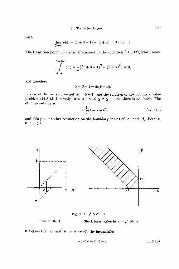
3. Transition Layers 277
with
lim v ( ~ ) = ( ~ + / 3 - 1 ) - ( ~ : + a ) = / 3 - a - 1 .
The transition point x = :~ is determined by the condition (11.3.14), which reads
&+fl-1 / 1
r/dr/= ~{ (2 4- fl - 1) 2 - (2 + a) 2 } = O,
and therefore
~ + ~ - 1 - + ( & + a ) .
In case of the + sign we get a = f l - 1 and the solution of the boundary value problem (11.3.15) is simply u = x 4 - a , 0 < x < 1 and there is no shock. The other possibility is
1 ~ - ~ ( 1 - a - ~ ) , (11.3.18)
and this puts another restriction on the boundary values of a and /3, because 0 < ~ < 1 .
tt
-!
~ ," t X --'t
Interior Shock
Fig. 11.1 fl > ce 4- 1
Shock layer region in a - fl plane
It follows that a and fl must satisfy the inequalities
4,'1
- 1 < a + fl < +1. (11.3.19)
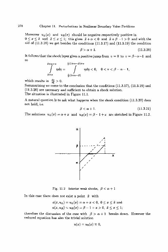
278 Chapter 11. Perturbations in Nonlinear Boundary Value Problems
Moreover UL(Z) and uR(z ) should be negative respectively positive in 0 < x < & and & < x < 1; this gives ~ + c ~ < 0 and & + 1 3 - 1 > 0 and with the aid of (11.3.18) we get besides the conditions (11.3.17) and (11.3.19) the condition
/3 > a + 1. (11.3.20)
It follows tha t the shock layer gives a positive j ump from v = 0 to v = r and S O
~+(~-t-v �89 (l+ot--,6)-I-v
I rldrl= f rldrl<O, i, +o, �89 (1+o,-~ )
which results in dv 7 > 0 .
O < v < f l - c ~ - l ,
Summariz ing we come to the conclusion tha t the conditions (11.3.17), (11.3.19) and (11.3.20) are necessary and sufficient to obtain a shock solution. The s i tuat ion is i l lustrated in Figure 11.1.
A na tura l question is to ask what happens when the shock condition (11.3.20) does not hold, i.e.
< c~ + 1. (11.3.21)
The solutions UL(X) = ~ + x and ult(:r) = 3 - 1 + x are sketched in Figure 11.2.
/
/ a
/ I
. . . . . -> ~--71 l I
/
4
Fig. 11.2 Interior weak shocks, fl < a + 1
In this case there does not exist a point $ with
a(x, uL) = UL(X) = a + x < O, O < x < ~c and
~(~, ~R) = uR(~ ) = ~ - 1 + �9 > 0, ~ < �9 < 1;
therefore the discussion of the case with ~ > c~ + 1 breaks down. However the reduced equat ion has also the trivial solution
u(~ ) = ~0 (~ ) -= 0,
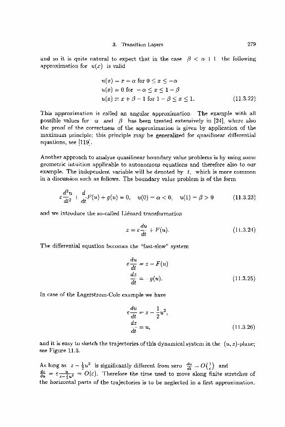
3. Transition Layers 279
and so it is quite natural to expect that in the case /3 < c~ + 1 the following approximation for u ( x ) is valid
u ( x ) = x + ol for 0 < x _< - a
u ( x ) -- O f o r - c ~ _ < x _ < 1 - / 3
u ( x ) -- x + ~ - l for l - /3 _< x _< l . (11.3.22)
This approximation is called an angular approximation. The example with all possible values for c~ and /3 has been treated extensively in [24], where also the proof of the correctness of the approximation is given by application of the maximum principle; this principle may be generalized for quasilinear differential equations, see [119].
Another approach to analyze quasilinear boundary value problems is by using some geometric intuition applicable to autonomous equations and therefore also to our example. The independent variable will be denoted by t, which is more common in a discussion such as follows. The boundary value problem is of the form
e-d-~ + d F ( u ) + g ( u ) = 0 u ( O ) = c ~ < O , u ( 1 ) = / 3 > O (11.3.23)
and we introduce the so-called Lidnard transformation
d u z = e- -~ + F ( u ) . (11.3.24)
The differential equation becomes the "fast-slow" system
d u e-d- [ = z - F ( u )
d z
d--[ = - g ( u ) . (11.3.25)
In case of the Lagerstrom-Cole example we have
du 1 ~--J-i = z - -~u 2,
d z
d-t - u, (11.3.26)
and it is easy to sketch the trajectories of this dynamical system in the (u, z)-plane; see Figure 11.3.
d~t 1 2 is significantly different from zero -&- As long as z - S u = O ( ~ ) and dz u = e z _ ~ 2 -- O(e). Therefore the time used to move along finite stretches of d-~
the horizontal parts of the trajectories is to be neglected in a first approximation.
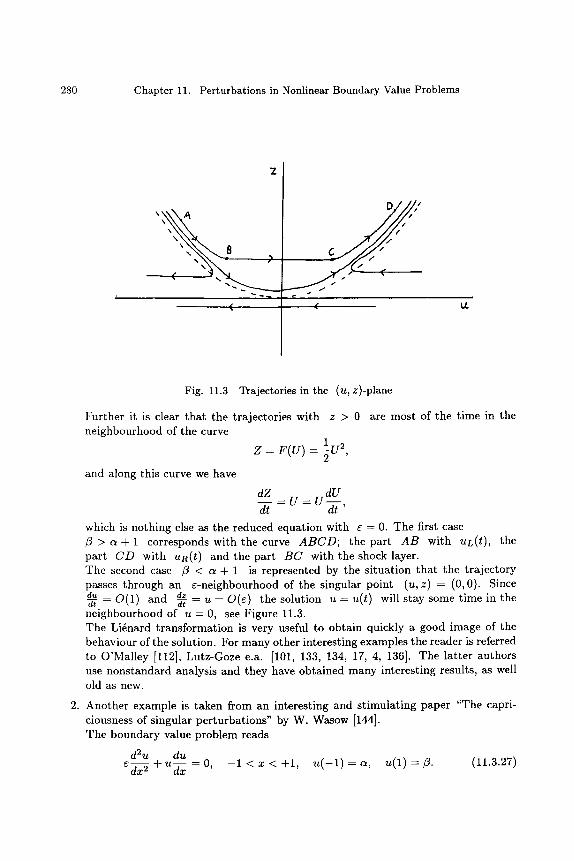
280 Chapter 11. Perturbations in Nonlinear Boundary Value Problems
D t
\ A~8 ""
\ \ \ �9 t /
>
ts
Fig. 11.3 Trajectories in the (u, z)-plane
Fur ther it is clear tha t the trajectories with z > 0 neighbourhood of the curve
and along this curve we have
1U2 Z = F(U) = -~ ,
are most of the t ime in the
dZ u d U ~ - V - -
dt d r '
which is nothing else as the reduced equat ion with ~ - 0. The first case /~ > c~ 4- 1 corresponds with the curve A B C D ; the par t A B with UL(t), the par t CD with uR(t) and the part B C with the shock layer. The second case ~ < c~ 4- 1 is represented by the s i tuat ion tha t the t ra jectory passes through an e-neighbourhood of the singular point (u, z) - (0, 0). Since
dz d~dt ---- O(1) and ~- -- u -- O(~) the solution u - u(t) will stay some t ime in the neighbourhood of u - - 0 , see Figure 11.3. The Li~nard t ransformat ion is very useful to obtain quickly a good image of the behaviour of the solution. For many other interesting examples the reader is referred to O'Malley [112], Lutz-Goze e.a. [101, 133, 134, 17, 4, 136]. The la t ter authors use nons tandard analysis and they have obtained many interesting results, as well old as new.
Another example is taken from an interesting and s t imulat ing paper "The capri- ciousness of singular per turbat ions" by W. Wasow [144]. The boundary value problem reads
d2u du ~-~ + u ~ = 0, - 1 < ~ < + 1 , u ( - 1 ) = ~ , ~ (1) = ~. (11 .3 .27)
3. Transition Layers 281
In case a < 0 and ~ > 0 the reduced equation has solutions
UL(X) = O~, --l <_ x < l, UR(X) ---- fl, --l < x <_ +l
and all point of the interval ( - 1 , + 1 ) have the property UL(X) < 0 and UR(X) > 0 and therefore we cannot apply the theory of this subsection. However, by Theorem 2 of section 10.3 both solutions might be considered as an approxima- tion of u(x). To decide which of the solutions UL(X) or UR(X) approximates u(x) depends on the possibility to construct an appropriate boundary layer in the neighbourhood of x = +1 in case we take u(x) ~ c~ < 0 or in the neighbourhood of x = - I in case we take u ( x ) . ~ > O . So let us assume that U L ( X ) - - a < O approximates u(x) for - - l _ < x < 1 and further that the boundary value u(1) = ~ is, for the time being, arbitrary; it may be positive, zero or negative. Stretching the x-coordinate in the neighbourhood of x = 1 by
l m x
C
gives for the boundary layer term v(~ c) the boundary value problem
d 2 (c~ + v) d(c~ + v) - ( c ~ + v ) ~ = 0 , 0 < ~ < c ~ ,
d~ 2 d~
with v ( 0 ) = ~ - c ~ a n d lim v(~ c ) = 0 .
Integration from ~ = +oo with -~(c~) -- 0 to some value of ~c gives
__dv _- _lv2(~ ) + av(~) d~ 2
(11.3.28)
and integrating once again with v(0) = / 3 - a yields the result
( 1 - x ) ~+,~2ae '~ 2aexp [ a L ~ ] v ( ~ ) = v = = . e e~e ~+~ - e x p [c~/-~] 1 1 . 3 . 2 9
( )
~-~ ~-~
To obtain in the case ~ > a a monotonically increasing boundary layer function v(~ c) and in the case ~ < a a monotonically decreasing one, it follows from the right-hand side of (11.3.28) that one should require ~ - a < - 2 a . Hence we get for
a + / 3 < 0 , a < 0 (11.3.30)
the approximation
u(x) ~ c~ + 2c~ ~+~ exp [c~L~] " (11.3.31) ~--c~
282 Chapter 11. Perturbations in Nonlinear Boundary Value Problems
In the same way it can be shown tha t for
a + / 3 > O , f l > O (11.3.32)
the solution of the boundary value problem (11.3.27) is approximated by
e x p [ - f l l ~ ] u(x) ,~/3 + 213 (~-~a+Z _ exp [ -/3---F]l+x "
The case a + fl = 0, a < 0 gives the approximat ion
(11.3.33)
u(x) ,~ a, - l _ < x < O a n d u ( x ) , ~ - a , O < x <_ 1,
and there is a t ransi t ion layer around x - 0. An easy calculation gives
2c~
u ( x ) ~ a - t , ' l + e x p [ ~j)ra~" - 1 < x < + 1 . (11.3.34)
As to the choice of the boundary values a and /3 the only case left is the case a > 0 and ~ < 0. By Theorem 2 of section 10.3 we cannot use the reduced equat ion with u ( - 1) = a or u ( + l ) = fl as s tar t ing point for the approximat ion of u(x) . The only escape is to use the trivial solution u ~- 0 of the reduced equat ion and we have
u(x) ~ O for - l < x < + l ,
and in general two boundary layers in the neighbourhoods of x = - 1 and x = 1.
We leave it to the reader to show tha t the approximat ion is given by
a u (~ ) ~ + (11.3.35)
~_ i+ . + 1 1 - - p l - - x " 2 ~ 2
It is interesting to note tha t one meets here an example with boundary layers which are not of exponential type. The dependence of the solution of our boundary value problem on the values of a and
is indicated in Figure 11.4. It is of interest to investigate also the t ransi t ion from one region to a neighbouring region in the a, /3 plane. Therefore one should make a and /3 dependent on ~, e.g. u ( - 1 ) = a - ~ and u ( + l ) = -c~ + r a < 0. For this the reader is informed in a paper by A. Boh6, using nons tandard analysis [15]; the boundary layer shifts as an initial layer from the right to the left.
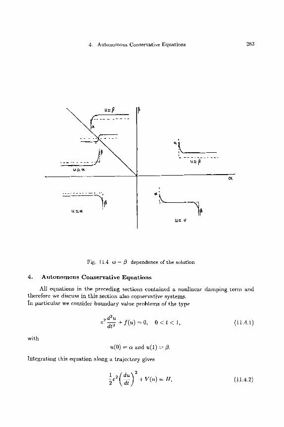
4. Autonomous Conservative Equations 283
. . . . . . . . . . . . . . . t
~ o t
!
l
!
Fig. 11.4 cz- f~ dependence of the solution
4. Autonomous Conservat ive Equations
All equations in the preceding sections contained a nonlinear damping term and therefore we discuss in this section also conservative systems. In particular we consider boundary value problems of the type
~2 d2u +f(u)=O, O < t < l , (11.4.1)
with
u(O) = c~ and u(1) = j3.
Integrating this equation along a trajectory gives
~2(du) 2 + v(~) = H, (11.4.2)
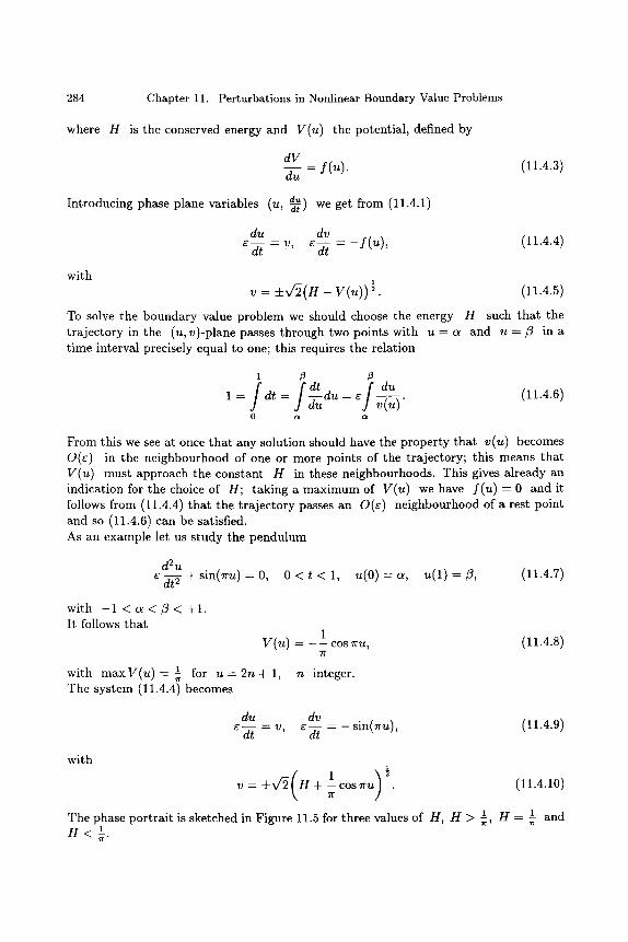
284 Chapter 11. Perturbations in Nonlinear Boundary Value Problems
where H is the conserved energy and V(u) the potential , defined by
dV du = f(u). (11.4.3)
Introducing phase plane variables (u d~ , -~-) we get from (11.4.1)
du dv ~-dt -- v, s--~ -- - f (u ) , (11.4.4)
with v : +v f2 (H- V(u))�89 (11.4.5)
To solve the boundary value problem we should choose the energy H such tha t the t ra jectory in the (u, v)-plane passes through two points with u = a and u = ~ in a t ime interval precisely equal to one; this requires the relation
i ,6 ,8
/ / d t d u / d u 1 = d t = - - d u = e . ~(u)
0 ~ ~
(11.4.6)
From this we see at once tha t any solution should have the property tha t v(u) becomes O(~) in the neighbourhood of one or more points of the trajectory; this means tha t V(u) must approach the constant H in these neighbourhoods. This gives already an indication for the choice of H; taking a max imum of Y(u) we have .f(u) = 0 and it follows from (11.4.4) tha t the t ra jec tory passes an O(~) neighbourhood of a rest point and so (11.4.6) can be satisfied. As an example let us s tudy the pendulum
d 2 u e-d-~- + s i n ( r u ) = O ' O < t < 1, u ( O ) = a , u ( 1 ) = ~ , (11.4.7)
with - 1 < a < ~ < + 1 . It follows tha t
1 V(u) = - - c o s r u , (11.4.8) 71"
1 for u = 2 n + l , with max V(u) = 7 The system (11.4.4) becomes
n integer.
du dv e-~- = v, e - ~ = - s in(ru) , (11.4.9)
with 1 ( 1 )2
v = +V/2 H + - cos r u . (11.4.10) 71"
1 H = 1 and The phase por t ra i t is sketched in Figure 11.5 for three values of H, H > 3, H < 1.
71"
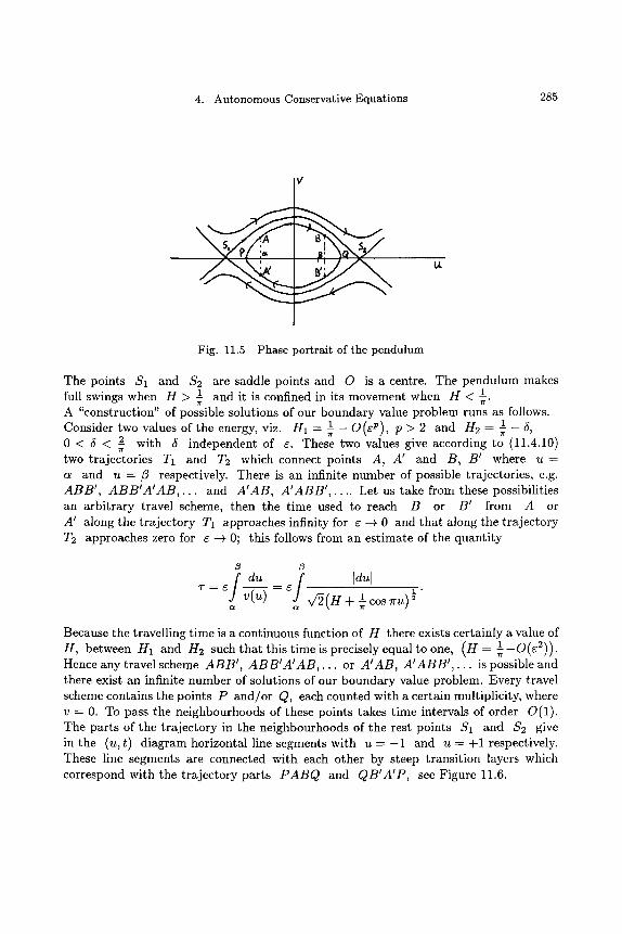
285
I V
\
4. Autonomous Conservative Equations
Fig. 11.5 Phase portrait of the pendulum
The points S1 and $2 are saddle points and O is a centre. The pendulum makes _ 1 full swings when H > 1 and it is confined in its movement when H < 3" 7r
A "construction" of possible solutions of our boundary value problem runs as follows. Consider two values of the energy, viz. HI = ~1 _ O(r p > 2 and H2 = 0 < 6 < _2 with 6 independent of ~. These two values give according to (11.4.10)
71"
two trajectories T1 and T2 which connect points A, A' and B, B' where u = a and u - fl respectively. There is an infinite number of possible trajectories, e.g. ABB', ABB'A'AB,... and A'AB, A'ABB',.... Let us take from these possibilities an arbi trary travel scheme, then the t ime used to reach B or B' from A or A' along the t rajectory Ti approaches infinity for c --+ 0 and tha t along the t rajectory T2 approaches zero for c -+ 0; this follows from an est imate of the quanti ty
j du f 1 u)�89 T = r V - - ~ = r v ~ ( H + ~ c o s o~ o~
Because the travelling time is a continuous function of H there exists certainly a value of 1 0 ( 8 2 ) ) . H, between HI and /-/2 such tha t this t ime is precisely equal to one, (H = ~ -
Hence any travel scheme ABB', ABB'A'AB,... or A'AB, A'ABB',... is possible and there exist an infinite number of solutions of our boundary value problem. Every travel scheme contains the points P and /or Q, each counted with a certain multiplicity, where v = 0. To pass the neighbourhoods of these points takes time intervals of order O(1). The parts of the t rajectory in the neighbourhoods of the rest points S1 and $2 give in the (u, t) diagram horizontal line segments with u = - 1 and u = +1 respectively. These line segments are connected with each other by steep transit ion layers which correspond with the t rajectory parts PABQ and QB'A'P, see Figure 11.6.
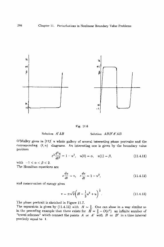
286 Chapter 11. Perturbations in Nonlinear Boundary Value Problems
"tt
§
= l
Fig. 11.6
Solution A ~ A B Solution A B B I A ~ A B
O'Malley gives in [112] a whole gallery of several interesting phase por t ra i ts and the corresponding (t, u) diagrams. An interesting one is given by the boundary value problem
~2 d2u -d-~ = 1 - u 2 ,
with - l < c ~ < f l < 2 . The Hamil ton equations are
du ~--~ -~ V~
and conservation of energy gives
u(O) = c~, u(1) =/3 , (11.4.11)
d ~ ) ~-~- = 1 - u 2, (11.4.12)
1 ( 1 U3 v = =t=x/2 H - ~ + u . (11.4.13)
The phase por t ra i t is sketched in Figure 11.7.
2 One can show in a way similar as The separatr ix is given by (11.4.13) with H - 5" 2 _ O(e2) an infinite number of in the preceding example tha t there exists for H = 5
"travel schemes" which connect the points A or A ~ with B or B ' in a t ime interval precisely equal to 1.
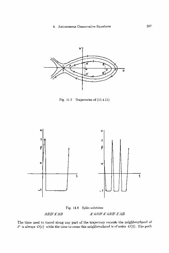
287
v I
4. Autonomous Conservative Equations
Fig. 11.7 Trajectories of (11.4.11)
tt
2. 2
--1
ABBtAIAB
Fig. 11.8 Spike solutions
A'ABBIA'ABBtAIAB
The time used to travel along any part of the trajectory outside the neighbourhood of P is always O(~) while the time to cross this neighbourhood is of order O(1). The path
288 Chapter 11. Perturbations in Nonlinear Boundary Value Problems
A B B I A p corresponds with a sharp spike in the (u, t) diagram, where u jumps during an ~-time interval from a to +2 and from +2 to c~; this is also in accordance with
1 (11.4.11) and (11.4.12) which gives a curvature of O(~) for u > - 1 +5, 5 independent of ~. A sketch of two possible solutions is given in Figure 11.8. For more l i terature on the interesting subject of this section we refer the reader to R.E. O'Malley [112, 113], and to R. Lutz and M. Goze [101], where is also t reated the nonautonomous case
._C2 d2u - ~ + f (t, u) = O, u(O)=c~, u ( 1 ) - - f l .
The lat ter authors use nonstandard analysis and they show in their book the s t rength of this method for many problems where a small or large parameter is involved. It is however outside the scope of this text to give an introduction to nonstandard analysis. Lutz and Goze present in [101] a ra ther general t rea tment of the boundary value problem (11.4.1) where V(u) may have any number of local minima and maxima, and they give also a formula for the location of the jumps.
5. A M o r e G e n e r a l C a s e
In this section we discuss a generalization of the boundary value problem (11.3.1)- (11.3.2). Instead of the semilinear equation (11.3.1) we consider now the equation
C~x2- - f u, dxx ' O < x < l , (11.5.1)
with u(0) = c~ and u(1) = ~.
We assume again tha t the reduced equation
(11.5.2)
f w, ~ = O, (11.5.3)
has a left solution WL(X) = g(x) for 0 < x _ ~ with g(0) = c~ and a right solution WR(X) = h(x) for ~ < x < 1 with h(1) = fl; moreover g(~) = h(2) = ~ and
r = ~-~(x) = #2. This means tha t the reduced equation has a so-called angular solution. We assume #1 < ~2 which is of course no restriction for what follows. The most fundamental paper on this boundary value problem is by Haber and Levinson, who discussed a generalization of the boundary value problem (11.5.1)-(11.5.2), [59]. They proved the following theorems for the boundary value problem
e-~x2 = f x , u , - ~ x , e , 0 < x < l , 0 < e < < l ,
with (11.5.4)
u(0) = a and u(1) = ft.
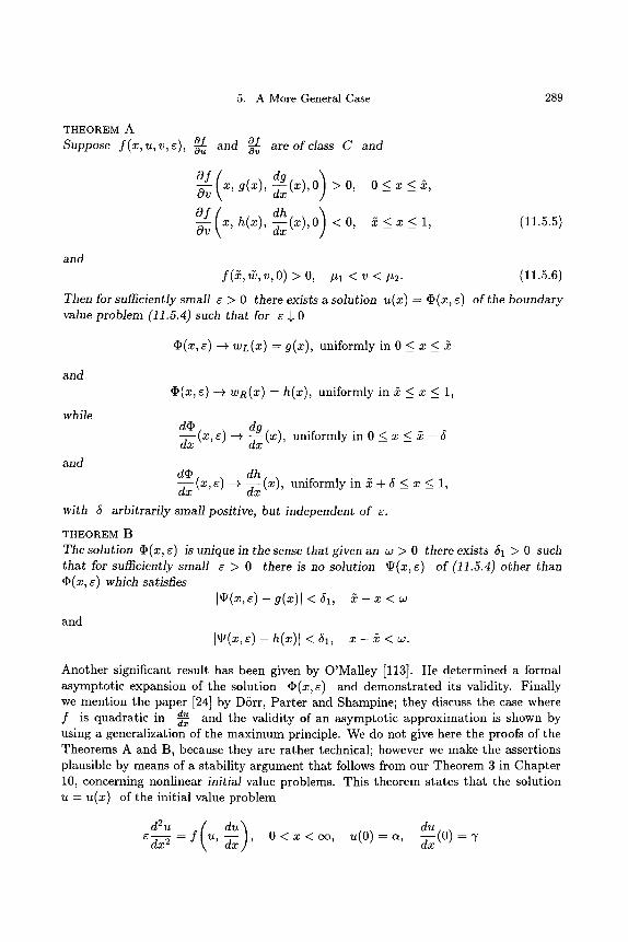
5. A More General Case 289
THEOREM A Suppose f (x ,u ,v ,e ) , ~ and ~ are of class C and
and
O f ( dg ) a~ ~ ' g ( ~ ) ' ~ ( ~ ) ' ~ > 0 , 0 < ~ < ~ ,
O f ( dh ) Ov x,h(x) , ~ ( x ) , 0 < 0 , ~_<x_< l, (11.5.5)
f (2 , ~, v, o) > o, ~ < v < ~2. (11.5.6)
Then for sumciently small e > 0 there exists a solution u(x) = O(x, e) of the boundary value problem (11.5.4) such that for ~ $ 0
O(x, e) -+ wi(x) = g(x), uniformly in 0 _< x _< ~:
and O(x,e) -+ wR(x) = h(x), uniformly in 2 < x < 1,
while dg
dO (x, e) --4 (x), uniformly in 0 < x < 2 - 5 dx dxx - -
and dO dh dx (x,r ~ --d-~x(x), uniformly in ~ + 5 < x < 1,
with 5 arbitrarily small positive, but independent of e.
THEOREM B The solution O(x, e) is unique in the sense that given an ca > 0 there exists 51 > 0 such that for sumciently small e > 0 there is no solution fig(x, r of (11.5.4) other than O(x, e) which satisfies
I~ , (~ ,~ ) - g(~)l < ,~, ~ - ~ <
and Ifig(X, E) --h(x)[ < ~1, x - ~ < w .
Another significant result has been given by O'Malley [113]. He determined a formal asymptotic expansion of the solution O(x, e) and demonstrated its validity. Finally we mention the paper [24] by D5rr, Parter and Shampine; they discuss the case where
du f is quadratic in ~ and the validity of an asymptotic approximation is shown by using a generalization of the maximum principle. We do not give here the proofs of the Theorems A and B, because they are rather technical; however we make the assertions plausible by means of a stability argument that follows from our Theorem 3 in Chapter 10, concerning nonlinear initial value problems. This theorem states that the solution u = u(x) of the initial value problem
d2u (du) e ~ x 2 = f u, ~ , O < x < c o , u ( O ) = a , ~xx(O)=9'
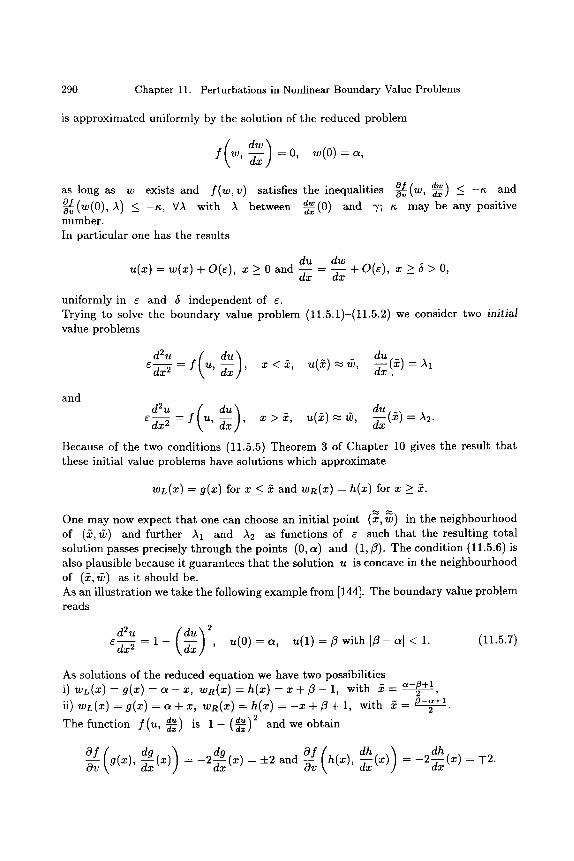
290 Chapter 11. Perturbations in Nonlinear Boundary Value Problems
is approximated uniformly by the solution of the reduced problem
( dw) f w, -~x --0' w(O)--o~,
as long as w exists and f(w, v) satisfies the inequalities -~(w, -~-~) < - ~ and d w ~ 0 ) 0 v , A) <_ - ~ , ~/A with A between -~-(0) and 7; ~ may be any positive
number. In particular one has the results
u(x) - w(x) 4- 0(~), x > 0 and du dw
= - - + O ( E ) , z >_ ~ > o, dx dx
uniformly in ~ and (f independent of ~. Trying to solve the boundary value problem (11.5.1)-(11.5.2) we consider two initial value problems
d2u ( d u ) du ~ x 2 -- f U,~xx , x < ~ , u ( ~ ) ~ , ~XX(;~)----)~I
i
and
~ x 2 - - f u, ~xx ' x > ~ , u(~) ~ , ~xx(X)--)~2.
Because of the two conditions (11.5.5) Theorem 3 of Chapter 10 gives the result that these initial value problems have solutions which approximate
wi(x) = g(x) for x <__ & and wR(x) = h(x) for x >_ ~.
One may now expect that one can choose an initial point (x, w) in the neighbourhood of (~, ~) and further )~i and ~2 as functions of ~ such that the resulting total solution passes precisely through the points (0, c~) and (1, ~). The condition (11.5.6) is also plausible because it guarantees that the solution u is concave in the neighbourhood of (~, ~) as it should be. As an illustration we take the following example from [144]. The boundary value problem reads
d2u (du) 2 e~-~x 2 - 1 - dxx , u(0)=c~, u ( 1 ) = ~ w i t h l f ~ - c ~ I < 1. (11.5.7)
As solutions of the reduced equation we have two possibilities i) WL(X)=g(x)=a--x, wR(x )=h(x )=x+~- l , with 2 = ~-#+i
2
ii) w L ( x ) - - g ( x ) = c ~ + x wR(x)=h(x )=-x+~+l , with ~ = ~-~+i , 2 "
The function f (u d~ d~ 2 ~--~) is 1 - - ( ) and we obtain ,
Of( d g ) ~ x x Of( d h ) dh Ov g(x), ~x(X) = - 2 (x) = 4-2 and ~v h(x), ~xx(X) = -2~xx(X) = ~=2.
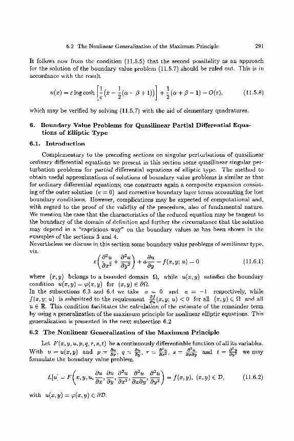
6.2 The Nonlinear Generalization of the Maximum Principle 291
It follows now from the condition (11.5.5) that the second possibility as an approach for the solution of the boundary value problem (11.5.7) should be ruled out. This is in accordance with the result
1 1 1 u ( x ) - c l o g c o s h ( x - ( c ~ - f l + l ) ) + ( c ~ + f l - 1 ) + O ( s ) , (11.5.8)
which may be verified by solving (11.5.7) with the aid of elementary quadratures.
6. B o u n d a r y Value P r o b l e m s for Quasil inear Partial Dif fe ren t i a l E q u a - t ions of El l ip t ic T y p e
6.1. Introduct ion
Complementary to the preceding sections on singular perturbations of quasilinear ordinary differential equations we present in this section some quasilinear singular per- turbation problems for partial differential equations of elliptic type. The method to obtain useful approximations of solutions of boundary value problems is similar as that for ordinary differential equations; one constructs again a composite expansion consist- ing of the outer solution (c = 0) and corrective boundary layer terms accounting for lost boundary conditions. However, complications may be expected of computational and, with regard to the proof of the validity of t h e procedure, also of fundamental nature. We mention the case that the characteristics of the reduced equation may be tangent to the boundary of the domain of definition and further the circumstance that the solution may depend in a "capricious way" on the boundary values as has been shown in the examples of the sections 3 and 4. Nevertheless we discuss in this section some boundary value problems of semilinear type, viz.
( 02u 02u ) Ou ~ OX 2 + ~ -~- a-~y + f ( x , y; u) -- 0 (11.6.1)
where (x, y) belongs to a bounded domain ft, while u(x, y) satisfies the boundary condition u(x, y) = ~(x, y) for (x, y) �9 0ft. In the subsections 6.3 and 6.4 we take a -- 0 and a - - 1 respectively, while
0I u) < 0 for all (x,y) �9 ft and all f ( z , y; u) is submitted to the requirement b-~ (x, y; u �9 ]R. This condition facilitates the calculation of the estimate of the remainder term by using a generalization of the maximum principle for nonlinear elliptic equations. This generalization is presented in the next subsection 6.2
6.2 T h e N o n l i n e a r G e n e r a l i z a t i o n of the M a x i m u m Principle
Let F(x, y, u, p, q, r, s, t) be a continuously differentiable function of all its variables. Ou Ou O2 u ~ u and t - 02 u With u - u ( x , y ) and p = b-~, q - ~yy, r - ~ , s = ~ ~ we may
formulate the boundary value problem.
( OU OU O2U O2U O2U) n[u] = F x, y, u, Ox' Oy' Ox 2' OxOy' Oy 2 = f ( x , y), (x,y) �9 7 : ) , (11.6.2)
with u(x, y) = ~(x, y) e 07).
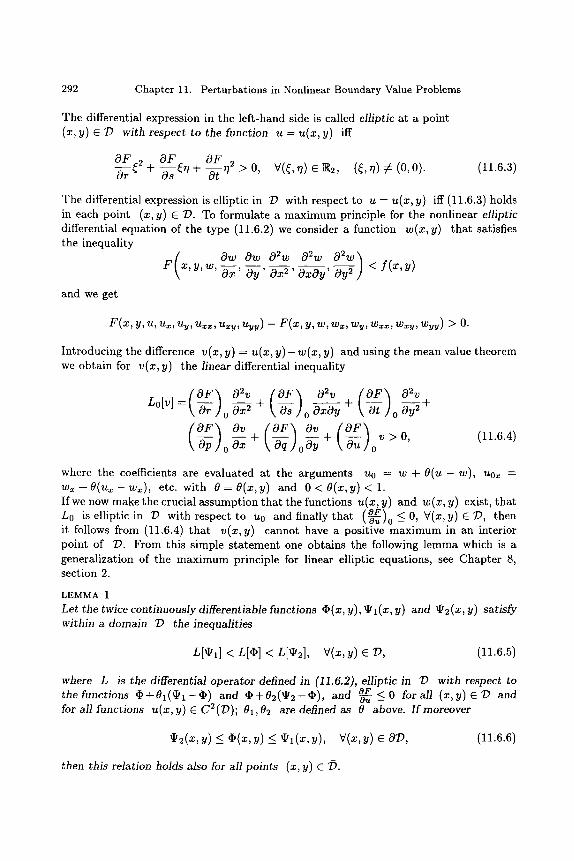
292 Chapter 11. Perturbations in Nonlinear Boundary Value Problems
The differential expression in the left-hand side is called elliptic at a point (x, y) e 1) with respect to the function u = u(x, y) iff
OF ~2 OF ~ OF z +~-;~ +-bY >0, V((, r/) �9 ]R2, (~, 77) # (0, 0). (11.6.3)
The differential expression is elliptic in 1) with respect to u = u(x, y) iff (11.6.3) holds in each point (x, y) C l). To formulate a maximum principle for the nonlinear elliptic differential equation of the type (11.6.2) we consider a function w(x, y) that satisfies the inequality
( OW OW 02W 02W 02W) F x , y ,w , Ox' Oy' Ox 2' OzOy' Oy 2 < f ( x , y )
and we get
F(x, y, u, u~, uy, u ~ , uxy, uyy) - F(x, y, w, wx, wy, wx~, w~v, wyy) > O.
Introducing the difference v(x, y) = u(x, y ) - w(x, y) and using the mean value theorem we obtain for v(x, y) the linear differential inequality
no[v] - ~ o-~-~-~x2+ ~ o o x o y + ~ o-~y2 +
N 0 ~ + oN + ~u oV>~ (11.6.4)
where the coefficients are evaluated at the arguments uo -- w + O ( u - w), uox - wx + O ( u x - wx), etc. with O= O(x,y) and 0 < O(x,y)< 1. If we now make the crucial assumption that the functions u(x, y) and w(x, y) exist, that L0 is elliptic in l) with respect to u0 and finally that (-b-4~)0~ _< 0, V(x, y) C ~9, then it follows from (11.6.4) that v(x ,y) cannot have a positive maximum in an interior point of :D. From this simple statement one obtains the following lemma which is a generalization of the maximum principle for linear elliptic equations, see Chapter 8, section 2.
LEMMA 1
Let the twice continuously differentiable functions ~(x, y), ~ l (x , y) and ~2(x, y) satisfy within a domain ~) the inequalities
L[~I] < L [ r < L[@2], V(x,y) E :D, (11.6.5)
where L is the differential operator defined in (11.6.2), elliptic in l) with respect to the functions ~ + 0 1 ( g 2 1 - ~ ) and ~ + 0 2 ( ~ 2 - ~ ) and OF < 0 for all (x ,y)ET~ and for all functions u(x, y) C C2(:D); 01,02 are defined as 0 above. I f moreover
�9 ~(~, y) < ~(~, y) < ~,(~, y), v(~, y) e or , (11.6.6)
then this relation holds also for all points (x, fl) C f).
6.3 Elliptic Equations without First Derivatives 293
The proof is simple; it is similar as the proof of the maximum principle for ordinary differential equations, as given in Lemma 2 of Chapter 7, section 2.2. Finally, we remark that the inequality (11.6.5) may be replaced by the sharper condition
L[~I] _< L[O] < L[ql2],V(x,y) e 7), (11.6.5")
see [119], Chapter 2, section 16 and Chapter 1, section 1.
If we want to apply this lemma to estimate the error in an asymptotic approximation of the solution of a singularly perturbed nonlinear boundary value problem we are ham- pered by the condition
OF _< 0, V(x,y) e T~, Vu e C2(D). (11.6.6)
Ou
This is rather serious as may already become clear from the following semilinear example
02u ~ Ou u) = O. aij(xl,x2, u, u~,, u~.2) OxiOxj + bi(Xl,X2, U)~xi + d(xl,x2,
i , j = l i= l
To be sure that OF < 0 one needs the restrictions that aij and bi do not depend on u and that Od <_ 0. The latter condition may be relieved a little bit; in case the coefficients {bi} do not depend on u one can use the trick of Remark 5 in Chapter 8, section 4 and the requirement Od < 0 may be replaced by the condition ~-~_
Od 3~1, ~)2, 5 E IR such that b i l l -F b2~2 + Ouu <- - 5 < 0, (11.6.7)
with t91,~2 and 5 independent of ~. The lemma holds of course also for ordinary differential equations; despite its limita- tions DSrr, Parter and Shampine showed its practical utility in their study of singular perturbations in nonlinear ordinary differential equations [24].
6.3 Elliptic Equations without First Derivatives
We study the boundary value problem
-5-~ ~+ oy~} + f ( ~ , y , ~ ) = 0, (x,y) Cgt, 0 < e < < l (11.6.8)
with the boundary condition
u(x, y) = ~o(x, y), (x, y) e O~t. (11.6.9)
We take Ft bounded and the data infinitely often differentiable with respect to their arguments. In particular, the parameter representation (x(a), y(a)) of OFt is smooth in a. In view of the application of the maximum principle we suppose
Of(x , y ,u )< 5 < 0 , V(x y) e ~ VuE]R. (11.6.10) Ou
294 Chapter 11. Perturbations in Nonlinear Boundary Value Problems
Finally, we assume tha t (11.6.8)-(11.6.9) has a solution and the same for the reduced equation
f(x,y,w) = 0 . (11.6.11)
It follows from (1.6.10) and the mean value theorem tha t this solution w is unique and the implicit function theorem gives w - w(x, y) with w E C ~ ( f t ) . In order to construct with the aid of w = w(x, y) an approximat ion ~ = fi(x, y) of the solution of (11.6.8)-(11.6.9) we have to introduce a boundary layer all along Oft, which takes care of the boundary condit ion (11.6.9). As in Chapter 8, formula (8.3.5) we introduce local coordinates (p, a) in an interior neighbourhood V of Oft; p denotes the distance PS from a point P E V to the boundary Oft and a the arc length from a given point So E Oft to the point S E Oft. Since Oft is smooth, the neighbourhood V can be defined as
0 _ p _ < p 0 , 0 _ < a _ a 0 , (11.6.12)
and there is in V a 1 - 1 correspondence between the coordinates (x, y) and (p, a). Let the pa ramete r representat ion of Oft be given by
then we have in V
x = x(a) + p - ~ 1+ ~(a) '
y = y ( a ) - p 1 + ~ - ~ , (11.6.13)
where the dots denote differentiation with respect to a and where one should pay a t tent ion to the right sign of the square root. Expressing our dependent variables in (p, a) we retain the nota t ion of our function symbols, e.g. f(x, y, u) with (x, y) e V is wri t ten as f(p, a, u). The differential equat ion (11.6.8) becomes in (p, a) coordinates
{ 02u 1 02u (02P 02p) Ou ( 020 -$Bp ~ + -~ ~ + -5~ ~ + -$~y ~ N + + oy~]~ +y(p,~,,u)-O,
(11.6.14) where J is the Jacobian
Ox
Stretching the coordinate p by p = V ~ T we obtain for the boundary layer function v(% a) in first approximat ion the boundary value problem
with
02v OT ~ - - + f (0, ~, ~ ( ~ ) + . ) = 0
v(O, a) = @(a) - t~(a) and lim V(T, a) = O, 7"--+OO
(11.6.15)
(11.6.16)
6.3 Elliptic Equations without First Derivatives 295
where ~(a ) = w(x(a), y(a)) and q3(a)= p(x(a), y(a)). With the aid of f(O,a, Cv(a)) = 0 and the mean value theorem it follows from (11.6.15)that
o~~ = O f (o, ~, ~(~) + O~)v Or 2 Ou
with 0 < 0 < 1 . It is in general not well possible to give an explicit formula for the boundary layer function v, but it is possible to establish its proper boundary layer behaviour. Because ~ < - 6 < 0 it follows that V(T, a) as function of T is concave for v > 0 and convex Ou for v < 0. As long as v(0, a) = ~ ( a ) - ~ ( a ) is not zero, it is impossible that the function v(~-, a) can change its sign for T > 0, because we have lim V(T, a) = 0. It follows
T---+ o O
that V(T, a) decreases monotonously for V(T, a) > 0, and increases monotonously for v(T,a)<O. Moreover for v(0, a ) > 0 we have due to v ( % a ) > 0 and ov ~(~, ~) < o
02v Ov Ov < 6 v ~
O~ "2 Or Or
It follows that
from which we obtain
< 5v 2 T
Integrating once again we get
OV OT
o~ or (0~T)2 T
> Sv 2 for T > O.
- - 0 - , ~) > a ~(~, ~).
~(~,~) = o(~ -~ ) = o ( ~ - ~ ) , (11.6.17)
which yields the exponential behaviour of the boundary layer term. Of course, the same reason holds for the case v(0, a) < 0. We consider now the function
P ~(~, y) - ~(~, y) + r ~), (11.6.18)
where r is a suitable C~176 off function, e.g.
1 3 r 0 ~ p < ~P0, and r _= 0, ~p0_~P_~P0,
with p0 as defined by (11.6.12). The function ~(x, y) is a formal approximation of the solution of the boundary value problem (11.6.8)-(11.6.9) and it satisfies by construction the boundary value problem
e ~ + ~ + f ( x , y , ~ ) - - O ( v ~ ) , uniformly in f , , (11.6.19)
296 Chapter 11. Perturbations in Nonlinear Boundary Value Problems
with
~(~, y ) [ o ~ = 0.
Put t ing
u(x, Y) -- u(~, Y) + R(x, Y)
we get for the remainder term R(x, y) the boundary value problem
~ \ o ~ + -g-~y~ + ~ -g-fi~ + -g-fiy~ + I (~,v, ~ + R ) - O, (~,v ) e a
with
Using (11.6.19) we obtain
R(~, V) l o~ = o.
02R 02R) r ~ + ~ + f ( x , y , ~ + R ) - f ( x , y , g ) = O ( v / e ) u n i f o r m l y i n a , (11.6.20)
R(~, V)[o~ = 0.
It is now not difficult to give by means of Lemma 1 an a priori estimate for the error R(x, y). Barrier functions are provided by taking ~1,2 = + K v / ~ with K sufficiently large. For ~1 - + K x / ~ we have
r + f (x ,y , fz + g~l) - f ( x y,~) : Of (x ~ +O1Kx/~)Kv~ < -e~Kx/~, ' -~u 'Y'
and similarly for ~2 = - K x / ~
eASe + f(x , y, fi + #2) - f (x , y, ~) > +5 KV~.
Hence R - - O ( v / ~ ) uniformly in ~ and we have the following theorem.
THEOREM 2 Let u(x, y) be the solution of the boundary value problem
h
with u(x, y) - ~o(x, y) along Of~ and suppose that the reduced equation
f(~, v, ~ ) = 0
has a solution in f~. Under the assumptions that all data are infinitely often differentiable and that
o~(~ , o f v,~) < -~ < o, v(~,v) e~, W E R
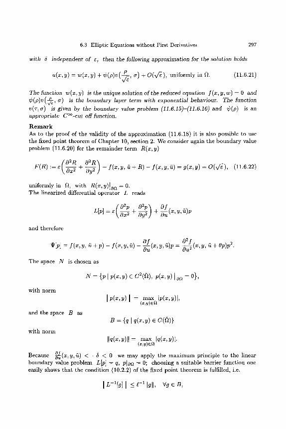
6.3 Elliptic Equations without First Derivatives 297
with 5 independent of e, then the following approximation for the solution holds
u(x,y) - w(x,y) + r a) + O(x/~), uniformly in ~. (11.6.21)
The function w(x, y) is the unique solution of the reduced equation f (x, y, w) = 0 and r -e- a) is the boundary layer term with exponential behaviour. The function v/~ v(T,a) is given by the boundary value problem (11.6.15)-(11.6.16) and r is an appropriate C~ off function.
R e m a r k As to the proof of the validity of the approximation (11.6.18) it is also possible to use the fixed point theorem of Chapter 10, section 2. We consider again the boundary value problem (11.6.20) for the remainder term R(x, y)
02R 02R) F(R) "= ~ ~ + ~ + f ( x , y , ~ + R) - f ( x , y ,~ ) - g(x,y) = O(v/~), (11.6.22)
uniformly in Ft, with R(x,y)log t = O. The linearized differential operator L reads
02p 02p~ Of L i p ] - r ~ + ~ ] + ~-~u (x, y, ~)p
and therefore
~o] = f(x, y, gz + p ) - f(x, y ~z) - Of 02f , ~u (x, Y, u)P : ~-U-gU2 (x, Y, u + Op)p 2.
The space N is chosen as
N = {p ip (x , y) C C2(Ft), p(x, Y) logt = 0},
with norm
and the space B as
with norm
I P(x,Y) [ = m a x Ip(x,y)l,
B - {qlq(x,y) e C(h)}
[[q(x, y)[[ = max_ [q(x, Y)I.
of 5) < - 5 < 0 we may apply the maximum principle to the linear Because O--4(x, y, boundary value problem Lip] -- q, Ploa - 0; choosing a suitable barrier function one easily shows that the condition (10.2.2) of the fixed point theorem is fulfilled, i.e.
]L-~[g]l ~ ~-lllgll, Vg ~ B,
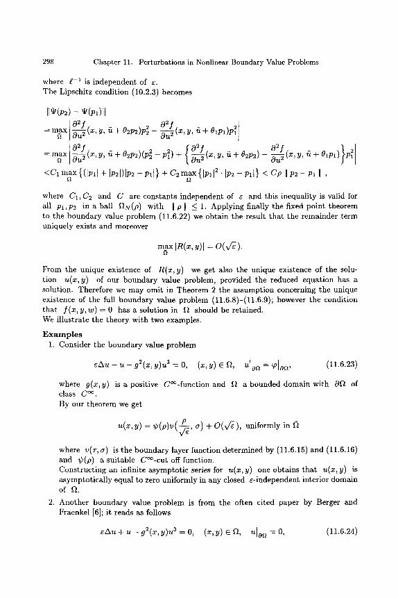
298 Chapter 11. Perturbations in Nonlinear Boundary Value Problems
where g-1 is independent of r The Lipschitz condition (10.2.3) becomes
I I r r 02 f 02.1 '
= m~x~ ~ (~, y, ~ + e~V~)V~ - ~ (~, y, ~ + 0~p~)Vl ~
02 f { 0 2 f , 02 f (x ft + Olpi) }p 2 = max~t ~ (x, y, ~t + 02P2)(P22 _ p2) + ~u2t.x ' y, (t + 02P2) - ~u 2 , Y,
< C 1 m a x {([Pl[ + [P2[)IP2 - Pll} + C2max {]pl[ 2- IP2 - Pll} < Cp IP2 - il91 I , f~ F~
where C1, C2 and C are constants independent of e and this inequality is valid for all pl, p2 in a ball ~N(P) with [ p] < 1. Applying finally the fixed point theorem to the boundary value problem (11.6.22) we obtain the result that the remainder term uniquely exists and moreover
max IR(x, Y)I = O(v/~ ).
From the unique existence of R(x, y) we get also the unique existence of the solu- tion u(x, y) of our boundary value problem, provided the reduced equation has a solution. Therefore we may omit in Theorem 2 the assumption concerning the unique existence of the full boundary value problem (11.6.8)-(11.6.9); however the condition that f (x , y, w) = 0 has a solution in ~ should be retained. We illustrate the theory with two examples.
E x a m p l e s 1. Consider the boundary value problem
~Au - u - g2(x ,y)u 3 = O, (x,y) e ~, u]og t = ~0]o~, (11.6.23)
where g(x, y) is a positive Coo-function and ~t a bounded domain with 0~t of class Coo. By our theorem we get
u(x ,y ) = r a) + O(v/~), uniformly in
where v(7,a) is the boundary layer function determined by (11.6.15)and (11.6.16) and r a suitable C~176 off function. Constructing an infinite asymptotic series for u(x, y) one obtains that u(x, y) is asymptotically equal to zero uniformly in any closed e-independent interior domain of ~.
2. Another boundary value problem is from the often cited paper by Berger and Fraenkel [6]; it reads as follows
~ + ~ - g~(~, y ) ~ = 0, (~, y) e ~, ~]o~ = 0, (11.6.24)
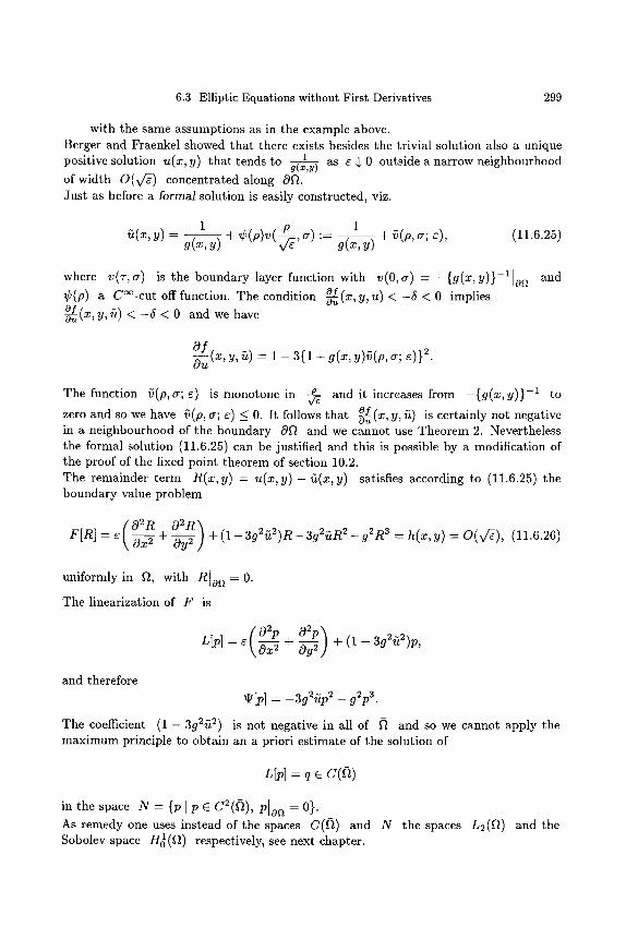
6.3 Elliptic Equations without First Derivatives 299
with the same assumptions as in the example above. Berger and Fraenkel showed that there exists besides the trivial solution also a unique
1 positive solution u(x, y) that tends to g-(E~,y) as e $ 0 outside a narrow neighbourhood
of width O(x/~) concentrated along 0Ft. Just as before a formal solution is easily constructed, viz.
s y) = g(x, y-------~ + r , a) "= ~ + ~(p, a; c), (11.6.25) g(~,y)
where v(T,a) is the boundary layer function with v ( O , a ) - - {g (x , y ) } - l ]o ~ and
r a C~ off function. The condition o~ y, u) < - 6 < 0 implies
~ y, ~) < - 6 < 0 and we have Ou
ol Ou (x,y,~) - 1 - 3{1 + g(x,y)~(p,a; ~)}2.
The function ~(p,a; ~) is monotone in ~ and it increases from - {g (x , y ) } -1 to
zero and so we have ~(p, a; ~) _< 0. It follows that ~ (x, y, ~) is certainly not negative in a neighbourhood of the boundary 0Ft and we cannot use Theorem 2. Nevertheless the formal solution (11.6.25) can be justified and this is possible by a modification of the proof of the fixed point theorem of section 10.2. The remainder term R(x,y) = u ( x , y ) - ~t(x,y) satisfies according to (11.6.25) the boundary value problem
02R ~)2R ~ FIR] = e -~x2 + -~y2 ] + ( 1 - 3g2~t2)R- 3g2(tR2 - g 2 R 3 = h(x, y) = O(x/~), (11.6.26)
uniformly in Ft, with RIo a = O.
The linearization of F is
02p 02p ) n [ p ] = e ~ + ~ + ( 1 - 3 g 2 ~ 2 ) p ,
and therefore V~[p] = _3g2~tp 2 _ g2p3.
The coefficient (1 - 3g2g 2) is not negative in all of ~t and so we cannot apply the maximum principle to obtain an a priori estimate of the solution of
L[p] - q E C(~t)
in the space N = {PIP E C2(~t), Ploct - 0}.
As remedy one uses instead of the spaces C(~) and N the spaces L2(Ft) and the Sobolev space H~(Ft) respectively, see next chapter.
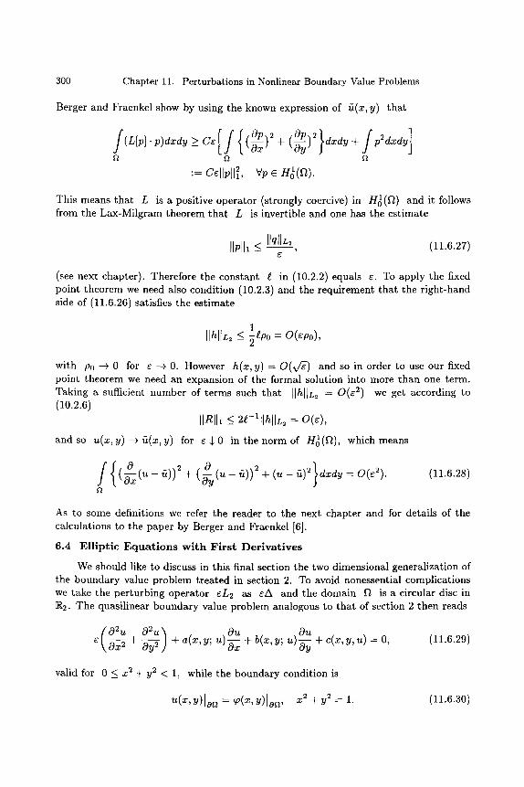
300 Chapter 11. Perturbations in Nonlinear Boundary Value Problems
Berger and Fraenkel show by using the known expression of fi(x, y) that
cOp ) 2 cOp 2 p2 dxdy]
s ~2 s
:= C~llpll~, vp e H,~(r~).
This means that L is a positive operator (strongly coercive) in H0~(f~) and it follows from the Lax-Milgram theorem that L is invertible and one has the estimate
Ilpll~ -~ IlqllL_____~, (11.6.27)
(see next chapter). Therefore the constant ~ in (10.2.2) equals e. To apply the fixed point theorem we need also condition (10.2.3) and the requirement that the right-hand side of (11.6.26) satisfies the estimate
1 IlhllL2 _~ ~ p o - O(~p0),
with p0 -+ 0 for e --~ 0. However h(x,y) -- O(vf~) and so in order to use our fixed point theorem we need an expansion of the formal solution into more than one term. Taking a sufficient number of terms such that Ilhlli2 = O(~ 2) we get according to (10.2.6)
IIRII~ _< 2~-~llhllL~ = O(~), and so u(x, y) -+ ~(x, y) for e $ 0 in the norm of H~(n) , which means
f { a (,., _ ,~))= a ( ._ ~))~ } ( ~ + ( ~ + (~- ~1~ e~dy = o(~1. ~2
(11.6.28)
As to some definitions we refer the reader to the next chapter and for details of the calculations to the paper by Berger and Fraenkel [6].
6.4 Elliptic Equations with First Derivatives
We should like to discuss in this final section the two dimensional generalization of the boundary value problem treated in section 2. To avoid nonessential complications we take the perturbing operator EL2 as eA and the domain f~ is a circular disc in R2. The quasilinear boundary value problem analogous to that of section 2 then reads
( 02~ 02~'~ O~ Ou \ o ~ + ~ ] + a(~, V; ~) ~ + b(~, V; u) ~ + c(~, y, ~) = O, (11.6.29)
valid for 0 < x 2 + y2 < 1, while the boundary condition is
x 2 y2 u(x, Y)lan = (p(x, Y)lon, + -- 1. (11.6.30)
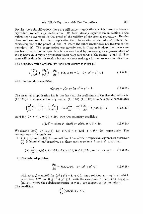
6.4 Elliptic Equations with First Derivatives 301
Despite these simplifications there are still many complications which make this bound- ary value problem very unattractive. We have already experienced in section 2 the difficulties to overcome in the proof of the validity of the formal procedure. Besides these we have now the extra complication that the solution of the reduced problem be- comes singular in the points A and B where the subcharacteristics are tangent to the boundary 0ft. This complication was already met in Chapter 8 where the linear case has been treated; an acceptable solution was found by presenting an approximation of the solution valid outside arbitrarily small neighbourhoods of the points A and B. The same will be done in this section but not without making a further serious simplification.
The boundary value problem we shall now discuss is given by
~ + 0y ~ ] - N + f (~ ' y; ~1 = 0, 0 < x 2 + y2 < 1 (11.6.31)
with the boundary condition
u(x, y) = ~(x, y) for x 2 + y2 = 1. (11.6.32)
The essential simplification lies in the fact that the coefficients of the first derivatives in (11.6.29) are independent of x, y and u. (11.6.31)-(11.6.32) become in polar coordinates
~02u l Ou 1 02u~ OOu e \ ~ + r N + ~ - ~ 0 0 2 ] - s i n Or
cos 0 0 u
r 00 ~- f(r, O, u) = O (11.6.33)
valid for 0 _< r < 1, 0 < 0 < 27r, with the boundary condition
u(1, 0) = ~o(cos 0, sin 0 ) : = ~o(0), 0 _< 0 < 2~r. (11.6.34)
We denote ~(0) by ~+(0) for 0 < 0 <_ 7r and 7r < 0 _< 27r respectively. The assumptions to be made are
1. f (x , y, u) and ~0(0) are smooth functions of their respective arguments; moreover -~ is bounded and negative, i.e. there exist constants 5 and ~ such that
Of < ~uu(r, 0, u) < 5 < 0 for 0 < r _ 1, 0 < 0 < 2r, - c ~ < u < +c~. (11.6.35)
2. The reduced problem
0~t) = f ( x , y, w), 0 < x 2 + y2 < 1 (11.6.36)
0y
with w(x,y)= ~_(0) for (x2+y 2) = 1, y < 0, has a solution w = wo(x,y) which is of class C ~ in 0 _ x 2 + y2 _~ 1 with the exception of the points (x, y) = (• 0), where the subcharacteristics x - +1 are tangent to the boundary.
The condition 0 / u - - 0 - ( ' ' ~ ' ~ < ~ < 0
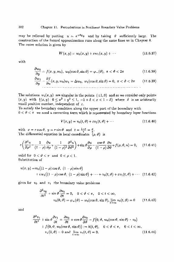
302 Chapter 11. Perturbations in Nonlinear Boundary Value Problems
may be relieved by putting u - e+~ and by taking 0 sufficiently large. The construction of the formal approximation runs along the same lines as in Chapter 8. The outer solution is given by
w(~ , v) = ~0(~, v) + ~ , ( ~ , v) + - (11.6.37)
with
OWo Oy
OWl Oy
= f ( x , y , wo), Wo(COSO, sinO) = ~o_(0), ~r < 0 < 2zr
Of (x, y, w0)w 1 ~-- AW0, W 1 (COS 0, sin 0) = 0, r < 0 < 2~ Ou
(11.6.38)
(11.6.39)
The solutions wi(x, y) are singular in the points (:t=1, 0) and so we consider only points (x,y) with {(x,y) 1 0 < x 2 + y 2 < 1, - l + 5 < x < 1 - 5 } where 5 is an arbitrarily small positive number, independent of e. To satisfy the boundary condition along the upper part of the boundary with 0 < 0 < ~ we need a correction term which is represented by boundary layer functions
v(~, v) = ~o(t, o) + ~v~(t, o) + . . . (11.6.40)
with x - r c o s 0 , y - r s i n 0 and t = 1-,- = e The differential equation in local coordinates (p, 0) is
02u 1 Ou 1 02u ) Ou cosO Ou+f (p ,O ,u ) 0 (11.6.41) Op 2 ( 1 - p ) Op t ( l - p ) 2 002 +s inOoo ( 1 - p ) Oz9
valid for 0 < 0 < 7 r and 0 < p < 1. Substitution of
u(x,y) =Wo((1 - p) cos0, (1 - p) sin0)
+ eWl((1 - p) cos0, (1 - p) sin0) + - . . + vo(t, zg) + evl(t, 0 ) + . . . (11.6.42)
gives for Vo and Vl the boundary value problems
02vo 073 0 +sinO~=O, 0<0<7r, O<t<oo, Ot---- ff-
vo(O, O) = ~o+(0) - wo(cos 0, sin 0) lim vo(t, 0) = 0 (11.6.43)
and
02Vl Ot 2
Ova Ovo ~ Ovo + sin 0 0--~ -- Ot + cos o - ~ - f (0, 0, wo(cos 0, sin 0) + vo)
+ f(O,O, wo(cosO, sinO)) :=h( t ,O) , 0 < 0 < Ir, O < t < cx~,
Vl(O,O)=Oand lim vl(t,O) = 0 . t--~ oo
(11.6.44)
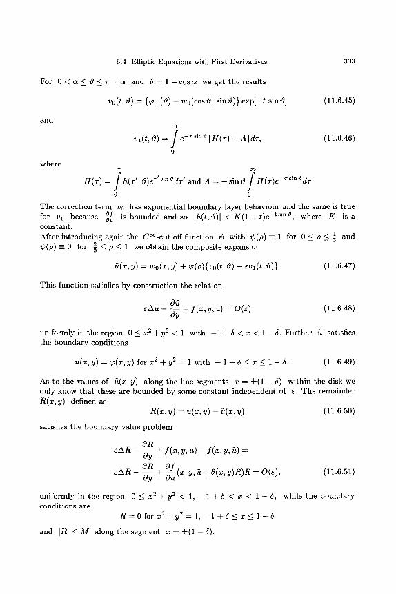
6.4 Elliptic Equations with First Derivatives 303
For 0 < c ~ < ~ ) < l r - c ~ and 6 = l - c o s c ~ we get the results
vo(t,~9) = {qa+(0)- w0(cos~9, sin0)} exp[- t sin~9] (11.6.45)
and
where
t
vl(t, 8) = J e-rsin~{H(T) + A}dT,
0
(11.6.46)
] J H(T) - h(T',~)eT'sin~dT ' and A = - s i n ~ H(T)e-rsin~dT
o o
The correction term v0 has exponential boundary layer behaviour and the same is true for Vl because ~ is bounded and so Ih(t, zg)l < g ( 1 + t ) e -tsin~, where g is a constant.
1 and After introducing again the C~-cu t off function r with r - 1 for 0 < p < 5 2 < < 1 we obtain the composite expansion r for ~ _ p _
~(~, y) = ~0(~, y) + r a) + ~v~ (t, a)}. (11.6.47)
This function satisfies by construction the relation
0~ ~ ' ~ - -z- + f ( x , Y, ~) - 0 ( ~ ) oy
(11.6.48)
uniformly in the region 0 < X 2 @ y2 < 1 with - 1 + 5 < x < 1 - 6. Further 5 satisfies the boundary conditions
~2(x ,y )=qo(x ,y ) fo rx 2 + y 2 - 1 w i t h - 1 + 5 _ < x _ < 1 - 6 . (11.6.49)
As to the values of ~(x, y) along the line segments x -- • - 6) within the disk we only know that these are bounded by some constant independent of e. The remainder R(x, y) defined as
R(x, y) - u(x, y) - ~z(x, y) (11.6.50)
satisfies the boundary value problem
OR eAR -~y + f (x , y, u ) - f (x , y, ~t) --
OR of eAR -~yy + -~u (X, y, ~z + O(x, y)R)R = O(e), (11.6.51)
uniformly in the region 0 < x 2 + y 2 < 1, - 1 + 6 < x < 1 - 6 , while the boundary conditions are
R - 0 f o r x 2 + y 2 - 1 , - 1 + 6 < x < 1 - 5
and IRI_<M along the segment x = + ( 1 - 6 ) .
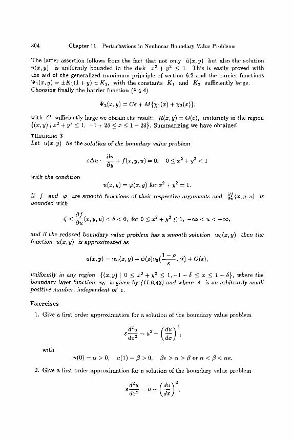
304 Chapter 11. Perturbations in Nonlinear Boundary Value Problems
The latter assertion follows from the fact that not only ~(x, y) but also the solution u(x, y) is uniformly bounded in the disk x 2 § y2 < 1. This is easily proved with the aid of the generalized maximum principle of section 6.2 and the barrier functions ~ l ( x , y ) - =kKl(1 + y) =t= K2, with the constants K1 and K2 sufficiently large. Choosing finally the barrier function (8.4.4)
~2(x,y) - Ce + M{Xl(X) + X2(x)},
with C sufficiently large we obtain the result: R(x, y) - O(e), uniformly in the region {(x, y ) [ x 2 + y~ _< 1, - 1 + 26 < x <_ 1 - 25}. Summarizing we have obtained
T H E O R E M 3
Let u(x, y) be the solution of the boundary value problem
~U r O<_x 2 + y 2 < 1
oy
with the condition u(x, y) = 9~(x, y) for x 2 + y2 = 1.
If f and ~ are smooth functions of their respective arguments and -~(x, y, u) is bounded with
of <: o u ( X ' y ' u ) < 6 < ~ fo r0<x 2+y2< 1, - e e < u < + c ~ ,
and if the reduced boundary value problem has a smooth solution wo(x, y) then the function u(x, y) is approximated as
~(~, y) = ~0(~ , y) + r - p 0) + o ( ~ ) s
uniformly in any region {(x,y) [ 0 _< x 2 + y 2 < 1 , - 1 + 6 < x _< 1 - 6 } , where the boundary layer function vo is given by (11.6.43) and where 6 is an arbitrarily small positive number, independent of e.
Exercises
1. Give a first order approximation for a solution of the boundary value problem
with ~(0) = ~ > 0,
d2U=u2 ( d u ) 2 ~-~ - ~ ,
u(1) = fl > 0, t 3 e > a > f l o r a < f l < a e .
2. Give a first order approximation for a solution of the boundary value problem
d2u (du) 2

Exercises 305
with 1 1
u ( 0 ) - a > 0 , u ( 1 ) = / 3 > 0 a n d 0 < x / ~ < ~, 0 < ~ <
Check the restrictions on the boundary values.
3. Give a generalization of Theorem 1 of this chapter by considering the following boundary value problem in an annular domain ft:
02U 10u 1 02u \ Ou + - + ) - a(~, ~, ~) + b(~, ~, ~) - 0 ," ~ -~-d-~ ~
0 < rl < r < r2, 0 ~ ~) < 2~r, with the boundary conditions
~(~ , o) - ~ ( ~ ) , ~(~ , ~) = ~ ( ~ ) .
The assumptions regarding the coefficients a, b and the boundary values T1 (0) and ~2 (~) are similar as stated in Theorem 1.

This Page Intentionally Left Blank
Chapter 12
P E R T U R B A T I O N S OF H I G H E R O R D E R
1. I n t r o d u c t i o n
In this final chapter we direct our attention to more general scalar perturbation problems. Up till now our perturbations were all of second order. A much more general situation is presented by the operator
r + L1, (12.1.1)
where L2 is a differential operator of arbitrary order m and L1 a differential operator of order k with 0 <_ k < m. To treat this kind of perturbation problems a more detailed specification is required. Whenever L2 may be of any order the same applies also to L1. As long as we deal with linear ordinary differential equations, boundary value problems are in general still tractable, but whenever we have to do with partial differential equations there is a plethora of problems. For instance L2 and L1 may be independently of each other elliptic, hyperbolic or parabolic and so there are already nine different cases of degeneration for r -=- 0 and in six cases we get a change of type of the operator. Apart from linearity or nonlinearity each problem requires its own theory, in particular if one wants to investigate the justification of a formal approximation of the solution. It is obvious that a general theory is not well possible and existing theories are far from complete. It seems sensible that the direction of research in the multitude of perturbation problems is to be determined by significant problems from mathematical physics, e.g. the equation of Navier-Stokes for the stream function, (in two dimensions). One of the most advanced texts presenting many boundary value problems with different degenerations is by J.L. Lions [100]; this author applies variational methods which are often used in modern textbooks on partial differential equations. Another important contribution is by M.I. Vi~ik and L.A. Lyusternik [138] treating boundary value problems for ordinary and partial differential equations, in particular the degeneration of an elliptic operator of higher order to one of lower order and the degeneration of an elliptic operator to one of first order. In connection with this paper we mention also the work by Besjes [9, 10, 11], who among other things improved the results by Vi~ik and Lyusternik by providing estimates in the maximum norm instead of the L2-norm. Further we refer the reader to the papers by D. Huet with L2 elliptic and L1 of order zero, [70, 71, 72] and by D. Huet [73] and W.M. Greenlee [55] with L2 and L1 both elliptic; these papers
308 Chapter 12. Perturbations of Higher Order
have been written in more or less the same spirit as in the book by Lions. Finally it is proper to mention also the well-known book by W. Wasow [139], where boundary value problems for ordinary differential equations have been treated.
A striking difference with perturbations of the second order lies in the circumstance that with second order problems a simple inspection of the differential equation gives a decisive answer to the question where to locate the boundary layer. This is no longer true for perturbations of higher order and it may even happen that a boundary layer construction induces severe complications, see [142].
It is outside the scope of this textbook to give an extensive t reatment of perturba- tions of higher order and therefore we restrict our considerations to the case of ordinary differential equations and to the case where both L1 and L2 are elliptic. In section 2 we deal extensively with boundary value problems for singularly perturbed ordinary differential equations. We investigate the location of the boundary layers and we give only a formal approximation. In section 3 we treat partial differential equations of elliptic type with an elliptic degen- eration and we use the variational method to obtain an approximation of the solution of boundary value problems in arbitrary bounded domains in ]~ . Using some theory of elliptic partial differential equations, it will appear that the construction of an approx- imation of the solution of the boundary value problem and the proof of its validity is very simple if we assume that the operators L1 and L2 are uniformly strongly elliptic and besides this that L1 is positive. Therefore we give first a short survey of the theory of elliptic equations stating the most important definitions and theorems; for proofs the reader is referred to well-known textbooks, e .g .A. Friedman [43] or S. Agmon [2]. One of the reasons to discuss the elliptic-elliptic degeneration is that it has a direct inter- esting application in the theory of thin shells. The boundary value for the displacement of a plate Ft, under lateral pressure and clamped along its edge OFt, reads
(~u r - Au = p(x, y), (x, y) C Ft with u[o a = -ff~n [Oa = O. (12.1.2)
This boundary value problem degenerates for 6 = 0 to the membrame problem with
- - A w -= p(x, y), (x, y) e Ft and W[o ~ - O. (12.1.3)
2. P e r t u r b a t i o n s of H i g h e r O r d e r in Ordinary Differential Equations
2.1 I n t r o d u c t i o n
We consider the following scalar boundary value problem with a perturbat ion of higher orer
Em-kLm[y] + L k [ y ] - f ( x ) , 0 < x < 1, (12.2.1)
where
dm "~ d m - i (12.2.2) Lm - dx---- ~ + E a i ( x ) dxm_---- ~
j--1
2.1 Introduction 309
and
dk k dk_ j (12.2.3) Lk = bo(x)~xk + E b j ( x ) dxk_ j ,
j = l
with bo(x) :/: 0 in [0, 1] and with the coefficients aj, bj and the right-hand side f infinitely often differentiable and finally 0 _< k < m; as boundary conditions we take
Bi[y](0) = ai , i - 1 , 2 , . . . r < m (12.2.4)
and
where
with
Bi[y](1)=j3i , i = r + l , r + 2 , . . . , r + s = m , (12.2.5)
d~,~ .x, - - 1 dj B~ = dx~------- 7 + E 7~J d-xxJ' (12.2.6)
j=o
0_<A1 < A 2 < ' . . < A r _ _ m - l a n d 0 _ < A r + l < A r + 2 < ' " < A m _ < m - 1
Our main task is to investigate the influence of the per turbat ion r on the solution of the reduced problem with ~ -- 0. But here we meet immediately the question how to define the reduced problem. In case k -- 1 and m - 2 one has the choice out of only two boundary conditons and a simple inspection of the unper turbed operator LI tells you which boundary conditon should be taken; in case bo(x) > 0 one fulfils the boundary condition at x - 1 and in case bo(x) < 0 the condition at x - 0. The choice of the proper boundary condition in the reduced problem is determined by the first term in the expansion of the operator r + L1 after the coordinate x has been stretched as x - r or x = 1 - r and it is the stability of the resulting boundary layer solution that fixes the proper choice of the boundary condition in the reduced problem. The same considerations apply also in the case m > 2, but it will appear tha t we get boundary layer equations at both end points of the interval [0, 1]. They read in first approximation
d m V d k V d m U d k U d~ m -[- b0(0) d--- ~ - = 0 and ( - 1 ) m~dr/m + (--1)kb0(1) ~ -- 0. (12.2.7)
The number of stable solutions determine the number of boundary layer corrections at each end point and hence also the number of boundary conditions left over for the reduced boundary value problem which, however, may not always be solvable.
2.2 The Formal Approximat ion
We return to our boundary value problem (12.2.1)-(12.2.6) and we shall give besides the construction of a formal approximation of the solution also the conditions under which this approximation is possible. The outer expansion
W(x; r E r (12.2.8) r t : O
310 Chapter 12. Perturbations of Higher Order
satisfies the recursive system
Lk[wo](X) = f (x),
Lk[w,] (x ) = O, n - l, 2, . . . (m - k - 1 ) ,
Lk[w,~](x) = -L ,~[wn-m+k] (x ) , n > m - k, (12.2.9)
valid for 0 < x < 1. Because we cannot state a priori the boundary conditions for W ( x ; e) we leave these open for the moment and remark only that each wn is determined by (12.2.9) up to any linear combination of k independent solutions of the homogeneous equation Lk[w] = O. Since W ( x ; e) cannot satisfy all m boundary conditions (10.2.4)-(10.2.5)we need boundary layer corrections at x = 0 or /and at x = 1. Stretching the x coordinate as x = e~ we get for the boundary layer function V(~; e) the equation
dm V d k V ,,~ d in_ iV k d k _ J v d~----- ~ + b o ( e ~ ) - ~ + E e J a j ( e ~ ) d~m_ j + E e J b j ( e ~ ) d~k_ j
j=l j=l
valid for ~ > 0. Expanding V(~; e) as
= 0 ,
oo
n = O
we get the recursive system
(12.2.10)
dmvo dkvo d~ m + b 0 ( 0 ) ~ = 0,
d~vn dkvn + b0(0) d--- ~ - - r=((), n > 1, (12.2.11) d( m
where r , ( ( ) is a linear combination of preceding terms ve and their derivatives (l < n) with coefficients being polynomials in (. The characteristic equation of the hemogeneous equation reads
A k (A m-k + b0(O)) = O, (12.2.12)
and we denote its roots with negative real part by /zj, j = 1, 2 , . . . q. It follows that the functions v~(~) with the right decaying boundary layer character are given by
and
q
vo(~) = ECjoe t 'J~ , (12.2.13) j = l
q
v , (~) = E ( c j , . , + ~p~)(~))e t'j~, (12.2.14) j = l
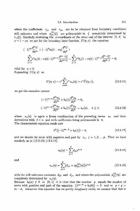
2.1 Introduction 311
where the coefficients Cjo and cjn are to be obtained from boundary conditions
still unknown and where _(1) Fin (~) are polynomials in ~ completely determined by rn(~). Similarly stretching the x-coordinate at the other end of the interval [0, 1] by x = 1 - er/ we get for the boundary layer function U(r/; e) the equation
(_ l )m dmU dkU d----- ~ + (-1)kb0(1 - er/)-~@ +
m k dm-Ju Ee jb j (1 1)k-J dk-jU E ~jaj(1 - er/)(-1)m-/&Tin--------7 + - er/) ( - d@-J
j = l j - - 1
= 0 ,
valid for r /> 0. Expanding U(~}; e) as
oo
u ( , ; ~ =
n = 0
(12.2.15)
we get the recursive system
(--1)m-k dmu0 d ku0 d~Tm -~- b0(1) d - ~ - -0 ,
(__l)m_kdmun dkun dr/---- ~ + b0(1) = s~(r/) d@
n _> 1, (12.2.16)
where sn(r/) is again a linear combination of the preceding terms ul and their derivatives with l < n and with coefficients being polynomials in 7}. The characteristic equation reads now
+ b0(1) ) = 0, (12.2.17)
and we denote its roots with negative real part by uj, j = 1, 2 , . . . p . Then we have similarly as in (12.2.13)-(12.2.14)
p
Uo(rl) = Edjoe~'Jn (12.2.18) j - - 1
and p
un(rl) - E (djn + rlp~.2) (rl))e ~'~'1 (12.2.19) j - - 1
_(2) with the still unknown constants dj0 and din and where the polynomials pin (~I) are completely determined by s,~O? ). Because bo(x) ~ 0 in [0, 1] it is clear that the number p equals the number of roots with positive real part of the equation (A m-k + b0(0)) = 0 and so p + q = m - k, whenever this equation has no purely imaginary roots; we assume that this is
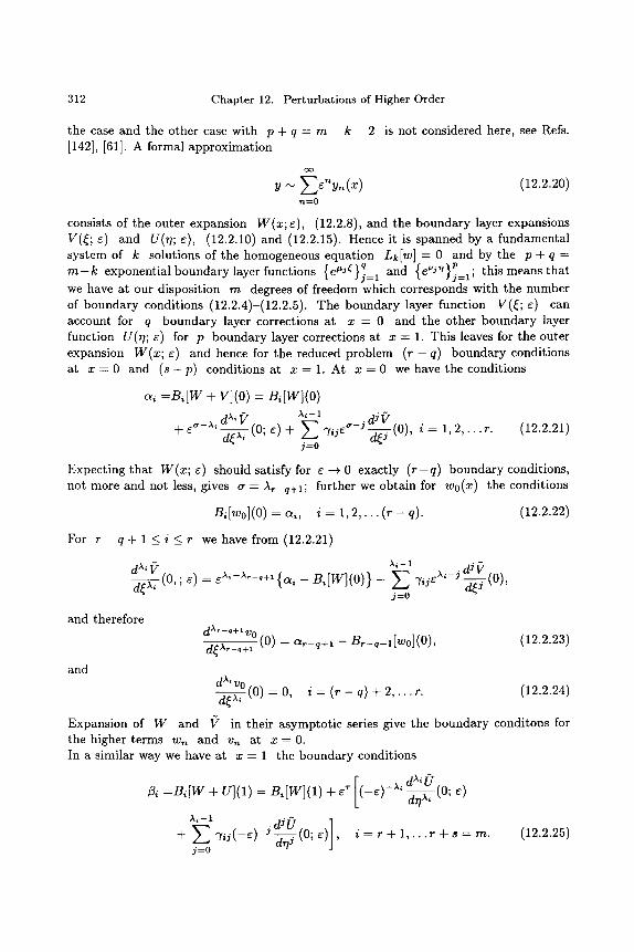
312 Chapter 12. Perturbations of Higher Order
the case and the other case with p + q -- m - k - 2 is not considered here, see Refs. [142], [61]. A formal approximation
oo
y ~ E e n y n ( x ) (12.2.20) n--0
consists of the outer expansion W ( x ; e), (12.2.8), and the boundary layer expansions V(~; e) and U(rl; e), (12.2.10) and (12.2.15). Hence it is spanned by a fundamental system of k solutions of the homogeneous equation Lk[w] = 0 and by the p + q = m - k exponential boundary layer functions {e t '~ } q and {e~ '}P=l �9 this means tha t
j = l we have at our disposition m degrees of freedom which corresponds with the number of boundary conditions (12.2.4)-(12.2.5). The boundary layer function V(~; e) can account for q boundary layer corrections at x = 0 and the other boundary layer function U(r/; e) for p boundary layer corrections at x = 1. This leaves for the outer expansion W(x; e) and hence for the reduced problem ( r - q) boundary conditions at x = 0 and ( s - p ) conditions at x = l . At x = 0 we have the conditions
~, : B i [ W + V](0) : Bi[W](0)
dX , Q ,~,- 1 dj i7 + e ~-~' (0; e ) + E 7 i J e ~ - J - ~ (0)' i = 1 2 , . . . r . (12.2.21) d~Xi
j=O
Expecting that W ( x ; E) should satisfy for e -+ 0 exactly ( r - q ) boundary conditions, not more and not less, gives a - At_q+1; further we obtain for wo(x) the conditions
Bi[wo](O) - c~i, i = 1, 2 , . . . (r - q). (12.2.22)
For r - q + l _ < i _ _ r we have from (12.2.21)
)~i--1 dj f / a~,d~, (" (o,, ~) = ~ ' -~-~+' { ~, - B,[W](O) } - ~ ~,j~'-J - ~ ( 0 ) ,
j = 0
and therefore
and
dXr-q+lvo d~Xr_q+l (0) - - O l r _ q + 1 - - Br-q+l[Wo](O), (12.2.23)
~ = B i [ W + U](1) = Bi[W](1) + ~ [(-r -x ' dX'[Td@' (0; e)
A,-1 dJU(0 ;e ) ] , i = r + l, . . r + s = m. + ~,j(-~l-J ~ j = 0
(12.2.25)
d X i VO ~ (o ) - o , i - (~ - q) + 2 , . . . ~ . ( 1 2 . 2 . 2 4 )
Expansion of W and V in their asymptotic series give the boundary conditons for the higher terms w,, and vn at x - 0 . In a similar way we have at x - 1 the boundary conditions
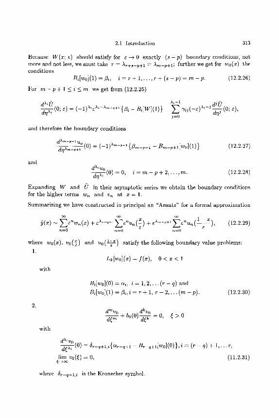
2.1 Introduction 313
Because W ( x ; e) should satisfy for e --+ 0 exactly ( s - p) boundary conditions, not more and rtot less, we must take ~- = At+s-p+1 - Am-p+1; further we get for w o ( x ) the conditions
B i [ w o ] ( 1 ) = /3i, i - r + l , . . . , r + (s - p) - - m - p. (12.2.26)
For m - p + l < i < m we get from (12.2.25)
,x,-1 dJ U (0; e) dAi~f ( 0 ; ~ ) = ( - - 1 ) A I ~ ) ' i - ) ' m - p + l { / 3 i - - Bi[W](1)} - E ~iJ(--~))ki--J drlAi
j=O
and therefore the boundary conditions
d),m-p+ l Uo d77Am_p+ 1 (0) = ( -1 ) Am-v+1 { f l m - p + l - B m - p + l [ W o ] ( 1 ) } (12.2.27)
and d Ai u 0 dr/A ' ( 0 ) = 0 , i = m - p + 2 , . . . , m . (12.2.28)
Expanding W and U in their asymptot ic series we obtain the boundary conditions for the higher terms w,~ and v~ at x - 1 .
Summarizing we have constructed in principal an "Ansatz" for a formal approximation
(x) oo oo
E n = 0 n = O n = 0
1 - x ) , (12.2.29) E
x ].--x where w0(x), v0(~) and u0(---/-) satisfy the following boundary value problems:
1. L k [ W o ] ( x ) = f ( x ) , 0 < x < 1
with
Bi[w0](0) - ai , i - 1, 2 , . . . (r - q) and
B i [ w o ] ( 1 ) - ~ i , i = r + 1, r + 2 , . . . ( m - p ) . (12.2.30)
with
d m v o dkvo + b0(0) -=- .~ - 0, ~ > 0
d~---- ~
d Aiv 0 d~Ai (0) -- ~r_q+l,i{o~r_q+l- Br_q+l[Wo](O)}, i - - ( r - q )+ 1 , . . . r,
lim v0(~) = 0, (11.2.31)
where (~r--q+l,i is the Kronecker symbol.
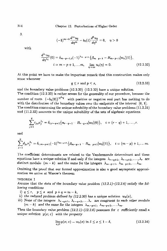
314 Chapter 12. Perturbations of Higher Order
with
(_l)m--k dmuo dkuo dr/---- ~ + b0(1)-~@ = O, r /> 0
d A' uo d@' (0) - 5m_p+l,i ( -1 ) am-p+' {Zm-p+l - Bm_p+l[wo](1)},
i = m - p + 1 , . . . m , lim u0(r/) = 0. ~/--4 oo
(12.2.32)
At this point we have to make the important remark that this construction makes only sense whenever
q < r and p < s, (12.2.33)
and the boundary value problems (12.2.30)-(12.2.32) have a unique solution. The condition (12.2.33) is rather severe for the generality of our procedure, because the
1 number of roots (-b0(0)) k with positive or negative real part has nothing to do with the distribution of the boundary values over the endpoints of the interval [0, 1]. The condition concerning the unique solvability of the boundary value problems (11.2.31) and (11.2.32) amounts to the unique solvability of the sets of algebraic equations
q
Ai = 6i,r_q+l{~r_q+l - - B r - q + l [ W o ] ( O ) } ECjo#j j = l
i = ( r - q ) + 1 , . . . , r .
and
P Edjo@' = 5i,m-p+l ( -1 ) x=-p+I { ] ~ r n - p + l - - Bm-v+l[w0](1)}, j = l
i = ( m - p ) + l , . . . m .
The coefficient determinants are related to the Vandermonde determinant and these equations have a unique solution if and only if the integers Ar-q+l, Ar_q+2,. . . , A~ are distinct modulo ( m - k) and the same for the integers A,~_p+l, Am-p+2,...A,~.
Omitting the proof that our formal approximation is also a good asymptotic approxi- mation we arrive at Wasow's theorem
T H E O R E M I
Assume that the data of the boundary value problem (12.2.1)-(12.2.6) satisfy the fol- lowing conditions
i) q<_r, p<_s and p + q = r a - k , ii) the reduced problem defined by (12.2.30) has a unique solution wo(x),
iii) None of the integers A~-q+l, A~_q+2,... A~ are congruent to each other modulo ( m - k) and the same for the integers A,,~-p+l, Am-p+2,. . . Am.
Th~n th~ boundary ~lue p~oblem (~2.2.~)-(~2.2.~) po~e~e~ ~o~ ~ ~umci,nt~y ~m~ll unique solution y(x; e) with the property
l i m y ( x ; e ) = w o ( x ) i n S < x < 1 - 5 , ~ $ 0 - - - -
(12.2.34)
3.2 Elliptic Partial Differential Equations 315
with 5 arbitrarily small positive, but independent of e. See also Wasow, Ref. [142, 139] or Vi~ik-Lyusternik [138]. The relevance of the conditions in this theorem is illustrated by the following examples, which we have taken from [139]
d4y dy ~ x 4 + dx = O, with y(O) = y'(O) = y" (0) - 0 and y(1) = 1,
d2y dy e dx----- 5 dx = O, with y' (0) = 1 and y.(1) - O,
d4y dy dx -----~ dx = O, with y(O) = y'"(O) = 0 and y(1) = O, y'(1) - 1.
It is not difficult to show that the solution of each of these boundary value problems has the property that y(x) diverges when e --+ +0. The reader can easily check that in each example one of the conditions of Wasow's theorem is violated.
An interesting and relatively simple example is given by the bending of a loaded elastic beam clamped at both ends.
3. Elliptic Perturbations of Elliptic Equations
3.1 Introduction
In this section we study singular per turbat ion problems involving equations of the type
eL2m[u] + L2k[u] = f(x). (12.3.1)
These problems are in a certain sense a generalization of the theory of the preceding section in so far as we consider now partial differential equations for functions depending on an arbitrary number of independent variables; however on the other hand the orders of L2k and L2m are restricted because we assume that both operators are uniformly strongly elliptic in their domain of definition. We include this type of problems in our discussion of higher order perturbat ions because it provides a simple and elegant application of the theory of elliptic partial differential equations. Because we need some functional analysis and some concepts which may not be familiar to the general reader, we give first a concise introduction to the theory of elliptic par- tial differential equations however without proofs; for these we refer the reader to the excellent treatise by Friedman [43] and also to the book by S. Agmon [2].
3.2 Elliptic Partial Differential Equations
3.2.1 Sobolev Spaces Let gt be an open set in ][~ and 0~t its boundary; cm(Ft) is the set of all
functions m times continuously differentiable in ~t and we denote by (~m(~t) the subset of cm(f't) consisting of all functions ~o E Cm(gt) with the finite norm:
1 { f~
1
�9 = I ~ l j (12.3.2)
316 Chapter 12. Perturbations of Higher Order
where a is a multi- index a = ( a l , a 2 , . . . , an); we denote
0 Dj = Oxj ~ , D s - D ~ ' D ~ 2 . . . D ~ " , lal = ~ a j and
j = l
s2 s , and a! a l ! a2 ! . . a , , w The completion of the Fur ther we write x s = x~ ix 2 . . . x n . . . . space (?m(~2) with respect to the norm (12.3.2) is called the Sobolev space Hm(f l ) . A
oo Cauchy sequence {~/}1 in (~m(fl) satisfies for 0 _ 1hi <_ m the relation
/ IDS~j - DS~kl2dx ~ 0 for j, k --+ co,
~2
and so, because L2(~) is a complete space, there exists a function u s �9 L2(~) such tha t
lim f lVS~oj - uSl2dx = O, (12.3.3) j -+oo
and this is valid for all a with 0 _< lal _< m. The function u s is called the s t rong derivative of order a of the function u �9 Hm(f l ) and we write u s = (DSu)8. Also the concept of weak derivative is useful. Whenever u and v are bo th locally integrable in
then v is called the weak derivative of u iff
/ uDS dx - (-1)J Jfv d , e (12.3.4) ~2 ~2
where C ~ is the subset of C~176 consisting of functions with compact suppor t in Q. We write v = (DSu)~. It can be shown tha t if u E L2(~) with a s trong derivative (DSu)8 then also (DSu)~ exists and they are equal. Also the converse is true: If u �9 L2(Q) has a weak derivative (DSu)~o then also (DSu)8 exists and again they are equal. According to the par t icular s i tuat ion both concepts may be used and we omit henceforth the suffix w or s. The space Hm(Q) is a Hilbert space with scalar product
(u,v)m= ~ (DSu, DSv)i2= ~ (12.3.5) Isl<_m Isl_<ma
where the bar denotes complex conjugation. Similarly the space H ~ ( f l ) is defined as the completion of the space C ~ ( f l ) with respect to the norm (12.3.2) and also H ~ ( f l ) is a Hilbert space with scalar product as defined by (12.3.5). Final ly we remark tha t we have the obvious inclusions Hm(~) C H k ( ~ ) and H~(~2) C H0k(~), k _< m.
3.2 Elliptic Partial Differential Equations 317
3.2.2 Ell ipt ic O p e r a t o r s , Bi l inear Forms and Ghrd ing ' s Inequa l i ty It will appear very useful to write our differential operators in the so-called diver-
gence form
L[u] = E (-1)IplDP(aP~ ' (12.3.6) 0<lPl,l~l<m
where we assume a pa to belong to C Ipl (gt) N cl~l(Ft). L is called strongly elliptic in ~t if there exists a positive function co(x) such that
Re{ E ~PaP~ >- c~ := c~ ~2 + ' " + ~ ) m , (12.3.7)
Ipl=l~l=m
for all ~C]R~ and all x C ~ . In case co(x) can be chosen independent of x then L is uniformly strongly elliptic and co is called the molulus of ellipticity. The formal adjoint L* of L is defined by
L*[v] = E (-1) I~ID~ (aP~(x)DPv) 0<lPl,l~l_<m
E (-1)IplDP(a~P(x) D~v)" O<[p[,[a[<m
(12.3.8)
For u, v C C ~ (gt) we have
with B[v, u] = E (DPv, aP~D~u) (12.3.9)
O<_lpl,l~l<~
Henceforth we write (v, u)0 - (v, u), the usual L2 scalar product. The expres- sion B[v, u] is called the bilinear form associated with L; this form is defined for ap~ bounded in ~ and for v and u belonging to Hm(Ft). This form satisfies the following theorem, important in the theory of elliptic partial differential equations, particularly for the proof of the existence of solutions of boundary value problems.
THEOREM A
Suppose that 1. L is strongly elliptic in a bounded domain f~ with modulus of ellipticity co, in-
dependent of x. 2. The coefficients a p~ are bounded in f~ for 0 <_ [p[, [a[ <_ m with upper bound
r
3. laP~(x)-ap~(y) l <_ c2( l~ -y l ) for I P l - Io l - m, for all x and y in f~, and c ~ ( l ~ - y l ) ~ 0 for I~ - yl ~ 0.
318 Chapter 12. Perturbations of Higher Order
Then there exist constants c and ko dependent on co, cl, c2 and ft such that
ReB[u, u] > c]lul] 2 - ko]lu]] 2 Vu �9 H g ( a ) m ~ "
(12.3.10)
This inequality is known as Gg~rdings inequali ty and a bilinear form satisfying (12.3.10) is called coercive. In the following we will suppose that the elliptic operators to be considered satisfy the three conditions stated above.
3 . 2 . 3 G e n e r a l i z e d D i r i c h l e t P r o l e m s We are interested in Dirichlet problems
L[u] = f in 12 C IR '~ (12.3.11)
with OJu 0uJ = gj in 09t, j = 0, 1 , . . . , m - 1, (12.3.12)
where L is an elliptic operator of order 2m and 12 is a bounded domain with boundary 012 of class C m-1. f and 9 are functions continuous in ~ and Oft respectively and o denotes differentiation in the direction of the outward normal of 012. If u E C2m(12)N Cm- l ( f i ) and if u satisfies (12.3.11)-(12.3.12) then u is a classical solution of the Dirichlet problem. In case 012 E C 2m+1 and 9j E C2m(012) the classical solution u is also determined by the classical solution of the homogeneous Dirichlet problem
L[v] = f* E 12, (12.3.13)
OJv = O i n O f t , j = O , 1 , . . . , m - 1 , (12.3.14)
OuJ
with v = u - �9 and f* = f - L[~], while ~ is an appropriate function belonging to O J ~ C2m((~) with the property ~ - 9j, J = 0, 1 , . . . , m - 1. It follows that it is not a too
strong restriction to discuss only homogeneous Dirichlet problems. We shall now generalize these problems in such a way that under certain conditions the solution of the generalized problem is also a classical solution; the advantage is that the proofs for existence and regularity of the solution become more transparant and elegant. The generalization of the differential equation L[u] = f is obtained by the associated bilinear form
B[~o, u] = (~o, f) , V~o G C ~ ( a ) ,
where the left-hand side is defined for u E H'~(ft) and derivatives up to only order OJu m are required. The generalization of the homogeneous boundary conditions ~ Ion =
0, j = 0, 1 , . . . , m - 1, is given by the assumption u E H~(gt) . This is justified by the following lemma.
L E M M A
0~ ~ = 0 for Suppose Oft is o f class C m. I f u E g ~ ' ( f t ) N cm-l(~'~), then -5-~[o~
oJ~ = 0 for O < j < m - 1 then 0 <_ j <_ r n - 1 ; also conversely, i f u E c m ( f i ) and -5-~]o~ - - '
3.2 Elliptic Partial Differential Equations 319
u C H~(gt) . These results lead to the following definition of a generalized solution of a homogeneous Dirichlet problem.
DEFINITION u is a generalized solution of the Dirichlet problem L[u] = f with homogeneous boundary conditions i f u C H ~ (f~) and
B[~, ~] = (V,/) , V~ e C3~ (12.3.15)
where B is the bifinear form associated with the differential operator L.
The problem to find a function u E H~(f~) that satisfies (12.3.15) is called the gener- alized Dirichlet problem The relation between a classical and a generalized solution is given by the following theorem
THEOREM B Let Oft be of c/ass C m and ap~ E clpl(~t). I f u is a classical solution of a homogeneous Dirichlet problem of order 2m with the property u E cm(~t) then u is also a generalized solution. Also conversely, i f u is a generalized solution belonging to Hg'(a) . nd with th~ p ~ o p ~ t y ~ c C 2 ~ ( ~ ) n C~- ' ( (~ ) the . ~ i~ ~1~o ~ c l ~ i c ~ l solution of the Dirichlet problem with homogeneous boundary conditions.
The consequence of this theorem is that the generalized solution yields also the classical solution whenever the data of the boundary value problem are sufficiently smooth.
3.2 .4 E x i s t e n c e of G e n e r a l i z e d S o l u t i o n s The existence of generalized solutions of Dirichlet problems with homogeneous
boundary conditions may be proved with the aid of the Lax-Milgram theorem, a gener- alization of the well-known representation theorem of Riesz. The lat ter reads as follows
THEOREM OF RIESZ Let H be a Hilbert space and let F[v] be a linear bounded functional on H, then there exists a unique element u C H such that
F[v] = (v, u).
The Lax-Milgram theorem is a generalization in so far as the scalar product (v, u) is replaced by the bilinear form B[v, u].
LAX-MILGRAM THEOREM Let there be defined on a Hilbert space H with norm [1" [[ a bilinear form B[v, u] with the properties.
i ) There exists a constant cl independent of v and u such that
IB(v, u)l < clllvll. Ilull, v,,,,., e H.
ii) There exists a constant c2 independent of v such that
[B(v,v)[ ~ c~ll~ll ~-, Vv e H.
320 Chapter 12. Perturbations of Higher Order
Then every bounded functional F[v] on H may be represented as
F[v] = B[v, ~},
with u uniquely determined by F.
An immediate consequence is the following existence theorem
THEOREM C If the bilinear form B[v, u] is bounded on H~(~t) and if there exists a positive constant c such that
ReB[v, v] > r w e Hg(f~) (12.3.16)
then the generalized Dirichlet problem
B[~a, u] = (~, f ) , V~ E C~(~t) , u e H~(f~) (12.3.17)
has for any f E L2(f~) a unique solution u with
I1~11,-,, < 1-11filL=. (12.3.18) C
The existence of the generalized solution follows from the Lax-Milgram theorem by taking F[v] = (v, f ) . The estimate (12.3.18) is obtained from (12.3.16) and the existence of a sequence { ~ } C C~( f t ) with lim ~ = u in H~(f t ) ; we have the inequalities
n - ~ o o
cllull~ ___ Re B[u, u] < IB[u, ~]1 = lim IB[~o., ~]1 n- - -# or
= lim [(So,-,, f ) [ - - (u, f ) < [[UiiL=- II/IIL= _< Ilu~ll. II/IIL= n - ' - + O0
and so the estimate (12.3.18) is obvious. A bilinear form that satisfies the inequality (12.3.16) is called strongly coercive in con- stant with coercive as defined by the Gs inequality (12.3.10). Regarding applications to elliptic boundary value problems it is important to give some examples of strongly coercive bilinear forms.
1. Let 12 be a bounded domain and L = - A + k with A the Laplace operator and k some positive constant. We have
B[v, u] = E (DPv' DPu) + k(v, u) Ipl=l
_ _ , _ _ . S - ~-5-&~_.dz + k vudx, [1
and therefore B[u, u] ~ rnin(1, k)llul[ 2.
3.2 Elliptic Partial Differential Equations 321
It follows tha t the boundary value problem
- ~ ( ~ ) + k~(~) - f (~ ) , ~ e a , ~1o~ - 0
has a unique generalized solution in H 1 for all f C L2(fl). This solution is also a classical solution if 0~t is of class C 1, u C C2(~) N C ( ~ ) and f C C(Ft) A L2(~t).
2. Let ~t be bounded and L = - A . To show tha t we have also in this case a s trongly coercive bilinear form we need the Poinca% inequali ty which may be applied to domains only bounded in one direction. This inequali ty reads
n
i1~11 ~ < d 2 2 ; d 2 ~ - ~ ' [ l O ~ - I 11 V~ C C~(Ft) (12.3.19)
i--1
where d is the maximal d iameter of ft. Suppose ft C {x C 1[~ []x~I < c}, then we have for ~ C C ~ ( f t )
X n
f O~ (x , x2 , x,~ ()d(. ~ ( ~ ) = ~-:~ 1 , . . . . ~, ~ C
Using Cauchy-Schwarz we get
+c +c
I~(x)l~ _< 2, Ib--~-~-(xl,x~.,...,-,~_l,e)l'd~=d Ib--~ 1 , . . . , x , _ l , - - C - - C
therefore +c +c
_< - - C ~ C
integrat ing once again with respect to XliX2,...,xn_ 1 we obtain (12.3.19). The bilinear form B[u, u] associated with L - - A satisfies according to (12.3.19)
n / Ou]2 1 2 1 Re B[u, u] = E ~ d~ = I-I~ > ~1-1~ + 7~ I "~
E L 2
i=0
1 1 _> min (~, ~-d--ff)ilull 2, Vu e H~(f~),
and so - A is s trongly coercive. We remark tha t + A does not yield a s trongly coercive bilinear form.
3. Let f~ be bounded and L = A 2. For any qo E C~(f~) we have the relat ion
i ~ ~ a "= J = l a
n n [ 02 ~ 2 2
i=1 j= l f~
322 Chapter 12. Perturbations of Higher Order
Applying the Poincar~ inequality to ~ we have cOx l
2
_< d 2 L2
and hence
n
i = 1
0~O ] 2 n < d2 ~"~
--ixi L2 -- i=1
2 n n
=d2EE 1 i = l j = l
02~
OxiOxj L2
Therefore we get for any q0 �9 C ~ (f~)
I1 11 = + + -< ( d~+ x)l~~ ~1 + I1,~,~. 2
_< {(d 2 + l )d 2 + l}l~, l~ = {(d ~- + 1)d 2 + 1}B[~o, ~o]
and we obtain by u = lim ~0,~ in Ho2(f~) the inequality n--~ r
Re B[u, u] = (Au, Au) > cllul[ 2, Vu �9 Ho2(f~),
from which the strong coercivity follows.
To give an example of a coercive but not a strongly coercive bilinear form we consider for U(Xl,X2) the boundary value problem
A u + # u - - 0 , 0 _ r = v / x 2 + x ~ < r o , # > 0 , w i t h u ( r o ) = 0 .
This problem has a nontrivial solution
= g 0 ( v ~ ) ,
if V/-fi r0 is a zero of the Bessel function J0. It follows that the boundary value problem
- - A u - - #u = f (xl ,X2), 0 ~ r < to, u(ro) = 0, # > 0
does not have a unique solution if v/-fir0 is a zero of J0 and therefore the strongly elliptic operator - A - # with J0 (v/-fi r0) - 0 cannot have a strongly coercive bilinear form. On the other hand it has a coercive bilinear form; this follows from Theorem A or by direct computation. As to existence of generalized solutions of coercive elliptic operators we have the following Fredholm alternative
T H E O R E M D
I f the differential operator L satisfies the conditions 1, 2, 3 of Theorem A and f E L2(~) then we have the next two possibilities
1. B[~o, u] - - (~o, f ) with ~o e C~(f~) has a unique solution u �9 H~(12), or
4.1 The Boundary Value Problem 323
2. there exists a finite number of linear independent solutions vj, j - 1, 2 , . . . g of the homogeneous equation
U[v, ~] = o, v~ e c g (a).
In this case B[qo, u] - (qo, f) has a solution i f and only i f ( f , vj) = O, j - 1, 2 , . . . ,g. This solution is not unique.
4 Elliptic Singular P e r t u r b a t i o n s of Higher Order
4.1 The Boundary Value Problem We study the following Dirichlet Problem for a real valued function u that satisfies
the partial differential equation
L~[u(x)] = ~L2m[u(x)] + L2k[U(X)] = h(x) , x e Ft C (12.4.1)
with the boundary conditions
~gu On t (x) = O, g = O, l, . . . m - 1 , x e OFt, (12.4.2)
where Ft is a bounded domain with boundary of class C ~176 The differential operators are given by
L2k - - E ( -1)IplDP(aP~(x)D~) ' (12.4.3)
o<lpl,l~l_<k
and L2m : E ( -1)IplDP(bP"(x)D~) ' (12.4.4)
O<_lPl,l~l<m
with 1 < k < m and where the coefficients a p'~, b p" are assumed real valued and of class C~ Moreover, L2k and L2m are uniformly strongly elliptic in ~ while L2k has a strong coercive bilinear form on the Sobolev space H0k(f~). Finally h(x) is also real valued, h E C ~ ( ~ ) and o denotes differentiation in the direction of the outward normal on 0Ft. Since all functions involved are real valued we consider in H0k(Ft) and H~(Ft) only real valued functions. The strong regularity conditions with respect to the data of the problem may be weak- ened; they have only been introduced to keep the exposition simple and a generalization is of course possible. Instead of the boundary value problem (12.4.1)-(12.4.2) we consider the generalized Dirichlet problem
eBm[~, u] + Bk[~, u] = e E (DP~~ bP~D~u) o<lpl,l~l<m
+ E (DPcp, aP"D"u) = (~, h), gqo �9 C~(f~), 0<lpl,l~l<k
(12.4.5)
324 Chapter 12. Perturbations of Higher Order
and it is our task to approximate the solution u C H~(f~) for e -+ O. This approxi- mation involves the solution w E H0k(f~) of the reduced problem
Blc[cp, w] = Z (D~ a~ - (~a, h), V~a e C ~ ( a ) . (12.4.6)
0<lol,lol<k
With the aid of a result concerning the regularity of solutions of generalized Dirichlet problems, see e.g. [43], Theorem 17.3, it follows from the regularity of our data that in case solutions u e H~(gt) and w e Hok(gt) exist, then these solutions belong also to C ~ ( ~ ) . Using consequently Theorem B of the preceding subsection we then get the result that u and w are also classical solutions of respectively the boundary value problem (12.4.1)-(12.4.2) and the reduced boundary value problem with e = 0 and the
boundary conditions ~ ~ ( x ) = 0, g = 0 , 1 , . . . k - I , x C 0s It follows that we may restrict our discussion to the study of the generalized Dirichlet problem.
4.2 Exi s t ence and A Priori E s t i m a t e We start with the following lemma.
LEMMA Whenever L2k has a strong coercive bilinear form on H~ then cL2m + L2k has also a strong coercive bilinear form on H ~ for e sufficiently small.
PROOF Gs inequality (12.3.10) gives for any v E Hy(f~)
Bm[v, v] = E (DPv' bP" (x)D" v) 0<lpl,l~l<m
>_ c~llvll~ - k~llvllo =,
where cm and km are constants with c,,, > O; [[vl[0 = [[Vl[L,(a). From the strong coercivity of Bk follows
Bk[v, v] = ( Dpv, aP"(x)D"v) > ckllvll~, O_<lpl,lal<k
valid for all v E H0k(Ft). Therefore we obtain for v e H ~ ( ~ ) C H~(fl) the inequality
sB,~[v, v] + Bk[v, v] >_ ~ l l v l l = ~ - ~k~ll~llo = + ~kll~ll~ >- ~11"11~ + ( ~ - ~k~)li~llg
1 _> ~ l l v l l ~ + ~ckllvll~ (12.4.7)
for e sufficiently small. Hence
~B.,[v, v] + Bk[v, v] > ~ l l v l l ~ ,
_ 1 c~ which proves the lemma. for O < e < e o - ~km,
4.3 The Approximation of the Solution 325
From the inequality (12.4.7) it follows tha t there exists a constant C = { min(cm, 1 -1 ~ck) } , which is independent of e, such tha t
Ivll~m + Ilvll~ ~ C{eBm[v, v] + Bk[v, v]}, (12.4.8)
valid for all v E H~(f~) and for 0 < e < e0. Henceforth we use the symbol C as a generic constant, independent of e, which may change its value without violating earlier results, where C has appeared.
The lemma has the following consequences 1. According to Theorem C the generalized Dirichlet problems (12.4.5) and (12.4.6)
have unique solution in H~(f~) and H0k(f~) respectively and due to the regulari ty of the da ta we have
u e H ~ (a) N C a (~) and w e H0 k (f~) M C a (~).
2. Wi th u = lim ~ in H~(f~) and ~,~ e C~(f~) we have from (12.4.8) n - - 4 ~
~ll~ll~ + II~ll~ _< C{~Bm[~, ~] + B~[~, ~]} = Cl i2~ {~B~[~ , u] + B~[~, ~]}
1 C 2 2 = C lira ( ~ , h) = C(u, h) < wllull 2 + IihiI L2 L2 n---+cx)
and therefore
ellull ~m + lull~ _ < Cl lh l l~ , (12.4.9)
where C is the generic constant independent of e. This relation yields an a priori es t imate for u and it appears tha t u and its strong derivatives up to and including order k are bounded in L2(f~) uniformly with respect to e. This is not necessarily true for the higher derivatives.
4.3 The Approx imat ion of the Solut ion It is na tura l to put
u(x) = w(x) + z(x) (12.4.10)
where w(x) is the solution of the reduced problem (12.4.6) corresponding with e - 0. Hence z C H0k(~t)N C~(Ft ) and z satisfies the equation
or in bilinear form
L~[z] = -~n~[~] ,
eBm[~V, z] + Bk[~, z] = - e ( ~ , L2m[w]), V~ e C ~ ( a ) (12.4.11)
It is impossible to es t imate z(x) with the aid of (12.4.9) because z does not belong to H ~ (f~). This follows from the loss of boundary conditions in w; therefore we introduce a correction te rm v with the proper ty tha t w + v belongs to H~(Ft) . In case we succeed we put
u(x) = w(x) + v(x) + 2(x), (12.4.12)
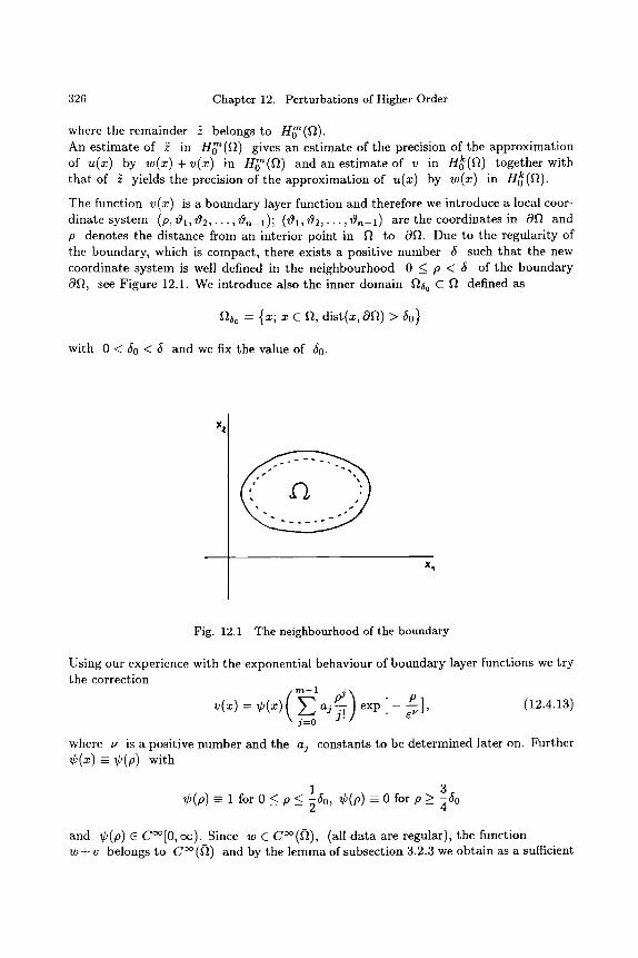
326 Chapter 12. Perturbations of Higher Order
where the remainder 5 belongs to H~(f~). An estimate of 5 in H~(f~) gives an estimate of the precision of the approximation of u(x) by w(x)+v(x) in H~(Yt) and an estimate of v in H0k(f~) together with that of ~ yields the precision of the approximation of u(x) by w(x) in H0k(f~).
The function v(x) is a boundary layer function and therefore we introduce a local coor- dinate system (p, 01, t92,.. . , 0n- l ) ; (v~l, 02 , . . . , 0,,-1) are the coordinates in 0f~ and p denotes the distance from an interior point in f~ to 0ft. Due to the regularity of the boundary, which is compact, there exists a positive number 5 such that the new coordinate system is well defined in the neighbourhood 0 < p < 5 of the boundary 0f~, see Figure 12.1. We introduce also the inner domain fl~o C fl defined as
f~o = {x; x c f~, dist(x, 0f~) > 50 }
with 0 < 5 0 < 5 and we fix the value of 50.
X~
X~
Fig. 12.1 The neighbourhood of the boundary
Using our experience with the exponential behaviour of boundary layer functions we try the correction
v(x) = r aj-fi, exp[ - - ~--~], (12.4.13) j=0
where u is a positive number and the aj constants to be determined later on. Further r - r with
1 3 r - 1 for 0 < p < ~ 0 , r - 0 for p > ~ 0
and r e C~ c~). Since w e C~ (all data are regular), the function w + v belongs to C ~ (~) and by the lemma of subsection 3.2.3 we obtain as a sufficient
4.3 The Approximation of the Solution 327
condition for w + v c H~(g t ) the following set of equations
Oe(w +v)[o=o = 0 for 0 < i < m - 1. Ope - _
(12.4.14)
The function w belongs to H0 k N C ~ (l)) and by the same lemma we get
O~w ,Io= o = 0 for 0 _< s _< k - 1. (12.4.15) Op e
Subst i tut ion of (12.4.13) into this equation gives immediately a0 = al = a2 . . . . . ak-1 - 0 and therefore
v ( x ) = r ( ~ l aj pj ) P j:k 7.1 exp [ -- ~--~]. (12.4.16)
Inserting this result into (12.4.14) yields a simple recursive set of ( r n - k) algebraic equations for the remaining coefficients ak, ak+l '"am-1. These equations read
l
j~ka j (~) (-1)e-J Oew ~. = k~ k + l m - 1 . (12.4.17) ev(e-j) = Ope Io=o' " ' "
- _ .
After solving we get the following est imates for aj
Okw ak = Opk [p=o = O(1)
Ok+lw ak ak+l = 0---~i Ip=o + (k + 1)~- V -- O(e -v )
Ok+2w a~+~ = 0p~+~ I,=0 + (k + 2)a~+~ (k + 1)(k + 2) a~ ~ 2 ~ = O ( ~ - ~ )
. . . . . . . . . . . . . . . . . . . . . . , etc.
Wi th the choice (12.4.17) we have (w + v) e H~(f~) and
aj - O(e-(J-k)v), j - k, k + 1 , . . . , m - 1. (12.4.18)
It will appear useful to have an est imate of the norm ]]vl] p in HP(f~). Because derivatives of r are only different from zero for 1/250 < p < 3//450, with 50 > 0 and independent of e, we have for e sufficiently small
Ilvjl 2 <_ c E ~ dl2
where C is independent of e.
328 Chapter 12. Perturbations of Higher Order
Put t ing p : e~T we get
Og " rn-- 1 T j OP eOev = r ~ [~(x) Z eJVaJ -j-(e-r] = O(e(k-e)u) ;
j = k
since the volume element df~ has a factor d p - r we obtain
(12.4.19)
Because w + v E H ~ (ft) and w e H0 k (it) the boundary layer term v belongs also to H0 k and it follows that
lim v = 0 in H0k; (12.4.20) e--~0
therefore this term is not "observable" for e small in the H0 k norm, but it becomes infinitely large in the H v norm for p > k.
4.4 T h e E s t i m a t e of t h e R e m a i n d e r a n d F i n a l R e s u l t s We have defined two remainder terms z(x) and 5(x) by
u(x) = w(x) + z(x) and u(x) = w(x) + v(x) + 5(x),
where w(x) is the solution of the reduced equation and v(x) the boundary layer term given by (12.4.16)-(12.4.17). In the following we give an a priori estimate of both remainders. From Le[z] = -eL2m[w] it follows that
eBm[~, z] + Bk[~o, z] = -e(~a, L2m[w]), V~ E C~(12).
Because C ~ ( a ) is dense in H~ ' ( a ) and 5 e H~'(fl) we get
eBm[5, z] + Bk[5, z] = - e ( 5 , Lzm[w])
o r
eBm[5, 5] + Bk[5, 5] = - e(5, L2m[w]) - eBm[5, z - 5 ] - Bk[5, z -- 5]
= - e(5, n2m[w]) - eBm[5, v ] - Bk[5, v]
< ~11~110 IIn~[~]ll0 + ~Cl]~ll~ I].11~ + CIl~llk I1,1]~-
With the aid of the estimate (12.4.19) there results the inequality
where C1 is again a generic constant independent of e. Because 5 e H g ( a ) we may apply the inequality (12.4.8)
zll~_<c~ [s, + [ s , s ] ,
Remarks 329
and therefore
~11~11~ + I1~11~ < c3{~11~110 + ~(k-m+�89 + ~�89
1 2el+(k_m+~)2vC 2 111~ 2 4e~,C2 1 -< { 4e2C2 + ~11~11~ + ~ + lira + + ~11~11~},
or after some reshuffling
ell~ll~ + II~ll~ < c 4 { F + el+2r,(k-m+�89 -4- er'}. (12.4.21)
The exponent u > 0 is still free and we make now an optimal choice such that the left-hand side becomes as small as possible; this is the case when
u = 1 + 2/2(k - m + 1), L
or (12.4.22)
1 / ] - - -
2 ( m - k)"
So we have finally obtained the a priori est imate
eli5]] 2 + 1]2,]]~ -- O(e2(:-k) ). (12.4.23)
The est imate for z follows from
~llzll~m + Ilzll~ __< ~11~11~ + I1~112 + ~llvll 2 + I1~112
and with the aid of (12.4.19) we get again
e]]z[] 2 + [[z[] 2 = O(e=(~- ' ) ). (12.4.24)
Summarizing our results we have proved
T H E O R E M 2
The boundary value problem (12.4.1)-(12.4.2) has for e sumciently small a unique solution u(x) and this solution is approximated by the solution w(x) of the reduced equation with e = 0. This approximation satisfies the relations
I lu- wllk - o (~<&~>) , l u - wllm -- o(~<d-~> ~). R e m a r k s
1. This result is ra ther weak, because the discrepancies between u and w are only in the L2 norm; sharper results are given in [73]. Pointwise approximations may be obtained by applying Sobolev's inequalities, see [43], [2]; further we refer the reader to [10].
2. Applications to thin plate bending problems are presented by Jiang Furu in [86]. 3. A generalization to certain quasilinear elliptic equations with elliptic-elliptic degen-
eration is possible, see [82].
330 Chapter 12. Perturbations of Higher Order
Exe rc i s e s
1. Give a formal approximation of the solution of the following boundary value prob- lems
d3u d2u du e~Sx3§ 0 , 0 < x < l ,
with the boundary conditions d~(1) = 1 a. u ( 0 ) = l , u ( 1 ) = 0 , ~ ,
du b. u ( 0 ) = 0 , a -~ (0 )= l , u ( 1 ) = l .
2. Give a formal approximation of the solution of the boundary value problem
dau du e dx 3 dx + u = O, 0 < x < 1,
du u(O) = 1, u ( 1 ) = O, ~xx(1)= 1.
3. Give an approximation of the solution of the following boundary value problem, regarding the deflection of an elastic beam
e 2 d a u d2u d x 4 d x 2 = f (x) , O < x < 1.
with the boundary conditions
u(O) = du du ~x(0) = u(1) = ~x(1) = 0.
Use as well the method of section 2 as that of section 4.
4. Consider the boundary value problem
eL2,T,[u(x)] + u ( x ) = h ( x ) , x e ~ C R,~
with ~gu On e (x) - O, g = O, 1, . . . , m - 1 , x E 0 ~ .
The operator L2m, the function h ( x ) and the domain fl are as defined in section 3.4.1.
R E F E R E N C E S
1 Ackerberg, R.C. and O'Malley, R.E., Boundary layer problems exhibiting resonance, Studies in Appl. Math., XLIX, No.3, 1970.
2 Agmon, S., Lectures in Elliptic Boundary Value Problems, Van Nostrand, Math. Studies, Vol.2, 1965.
3 Arnold, V.I., Mathematical Methods of Classical Mechanics, Springer, Berlin, 1978.
4 Benoit, E., Equation de Van der Pol avec 2e terme forr Publ. IRMA, D6p. de Math6m., Univ. Louis Pasteur, Strasbourg, 1979.
5 Berg van den I., Nonstandard Asymptotic Analysis, Springer Lecture Notes in Math., 1249, Berlin, 1987.
6 Berger, M.S. and Fraenkel, L.E., On the asymptotic solution of a nonlinear Dirichlet problem, J. of Math. and Mech., 19, no.7, pp. 553-585, 1970.
7 Bergmann, P.G., Introduction to the Theory of Relativity, 10th printing, Prentice Hall, Englewood Cliffs, 1960.
8 Bers, L., John, F. and Schechter, M., Partial Differentia/Equations, Lectures in Applied Mathematics, III, Intersc. Publ., New York, 1964.
9 Besjes, J.G., Singular Perturbation Problems /'or Partial Differential Equations, Thesis, Technical University of Delft, 1973; see also J. Math. Anal. Appl. 48, pp. 594-609, 1974 and 49, pp. 24-46, pp. 324-346, 1975
10 Besjes, J.G., Singular perturbation problems for linear elliptic operators of arbitrary order, I, degeneration to elliptic operators, J.Math. An. and Appl. 49, pp. 24-46, 1975.
11 Besjes, J.G., Singular perturbation problems for linear elliptic operators of arbitrary order II, degeneration to first order operators, J. Math. An. and Appl., 49, pp. 324-346, 1975.
12 Blondel, J.M. t~tude de deux probl6mes singuliers relatifs aux 6quations aux d6rivfes partielles, lin6aires et hyperboliques du second ordre, J. Math. Pures Appl (9), 40, pp. 247-299, 1961.
13 Blondel, J.M., Peturbation singuli6re pour une 6quation aux d6riv6es partielles du second ordre, lineaire, du type hyperbolique normal, C.R. Acad. Sc. Paris, 257, pp. 353-355, 1963.
14 Bogoliubov, N. et Mitropolski, I., Les Methodes Asymptotiques en Thdorie des Oscillations Non Lineaires, Gauthier-Villars, Paris, 1962.
332 References
15 Boh4, A., Free layers in a singularly perturbed boundary value problem, SIAM J. Math. Anal, 21, no.5, 1990.
16 Bruijn de, N.G., Asymptotic Methods in Analysis, 2nd ed., North- Holland Publ. Cy, Amsterdam, P. Noordhoff, Groningen, 1961.
17 Callot, J.L., Diener, F., Diener, M., Chasse au Canard, Publ. IRMA, D4p. de Math4m., Univ. Louis Pasteur, Strasbourg, 1977; Comptes Rendus Ac. Sc., t.286, 1978.
18 Chikwendu, S.C. and Kervorkian, J., A perturbation method for hyperbolic equa- tions with small nonlinearities, SIAM J. Appl. Math., 22, 2, 1972.
19 Cole, J.D., Perturbation methods in applied mathematics, Blaisdell, Waltham, Mass, 1968.
20 Cole, J.D., The development of perturbation theory at GALCIT, SIAM Review, 36, 3, pp. 425-430, 1994.
21 Cook, L.P. and Ludford, G.S.S., The behaviour as r --~ 0 + of solutions to eV2w - o (b-~y)w on the rectangle 0 < x < ~, [y[ <_ 1, SIAM J. Math. Anal, 4, 1,
pp. 161-184, 1973.
22 Copson, E.T., An Introduction to the Theory of Functions of a Complex Variable, Oxford University Press, 1948.
23 Courant, R. and Hilbert, D., Methods of Mathematical Physics, vol 2, Interscience, New York, 1962.
24 Dhrr, F.W., Parter, S.V. and Shampine, L.F., Application of the maximum principle to singular perturbation problems, SIAM Review, 15, 1, pp. 43-88, 1973.
25 Dodd, R.K., Eilbeck, J.C., Gibbon, J.D. and Morris, H.C., Solitons and Nonlinear Waves, Academic, London, 1982.
26 Dyke Van, M., Perturbation Methods in Fluid Mechanics, The Parabolic Press, Stanford, 1975.
27 Dyke Van, M., Nineteenth-century roots of the boundary layer idea, SIAM Review, 36, 3, pp. 415-424, 1994.
28 Dzavadov, M.G., A mixed problem for a hyperbolic equation involving a small parameter with the leading derivatives, Soviet Math. Doklady, 4, pp. 1400-1404, 1963.
29 Eckhaus, W. and de Jager, E.M., Asymptotic solutions of singular perturbation problems for linear differential equations of elliptic type, Arch. Rat. Mech. and Anal., 23, pp. 26-86, 1966.
30 Eckhaus, W., Asymptotic Analysis of Singular Perturbations, North- Holland Publ. Cy, Amsterdam, 1979.
31 Eckhaus, W., New Approach to the Asymptotic Theory of Nonlinear Oscillations and Wave Propagation, J. Math. An. and Appl., 49, pp. 575-611, 1975.
32 Eckhaus, W. and Garbey, M., Asymptotic analysis on large timescales for singular perturbations of hyperbolic type, SIAM J. Math. Anal., 21, pp. 867-883, 1990.
33 Eckhaus, W., Fundamental Concepts of Matching, SIAM Review, 36, pp. 431-439, 1994.
References 333
34 Esham Jr, B.F., A singularly perturbed Cauchy problem for an evolution equation in Hilbert space, Diss. University of Delaware, 1982.
35 Esham Jr, B.F., A singularly perturbed second order evolution equation with non- local nonlinearity, Num.Funct.Anal. and Optimiz. 9, (9-10), pp. 969-986, 1987.
36 Esham Jr, B.F., Asymptotics and an asymptotic Galerkin method for hyperbolic- parabolic singular perturbation problems, SIAM J. Math, Anal., 18, pp. 762-776, 1987.
37 Esham Jr, B.F., A hyperbolic singular perturbation of Burgers' equation, preprint, Dept. of Math. Sc., Virginia Commonwealth University, Richmond, Virginia.
38 Esham Jr, B.F. and Greenwell Yanik, E., Galerkin methods for a singularly per- turbed hyperbolic problem with nonlocal nonlinearity, prepr. Dept. of Math. Sc., Virginia Commonwealth University, Richmond, Virginia.
39 Esham Jr, B.F. and Weihnacht, R.J., Hyperbolic-parabolic singular perturbations for scalar nonlinearities, Applicable Anal., 29, pp. 19-44, 1988.
40 Esham Jr, B.F. and Weihnacht, R.J., Hyperbolic-parabolic singular perturbations for quasilinear equations, preprint Dept. of Mathem. Sci., Virginia Commonwealth University and Dept. of Mathem. Sci., University of Delaware.
41 Fife, P.C., Semi-linear elliptic boundary value problems with small parameter, Arch. Rat. Mech. Anal. 52, pp. 205-232, 1974.
42 Frankena, J.F., A uniform asymptotic expansion of the solution of a linear elliptic singular perturbation problem, Arch. Rat. Mech. and Anal. 31, pp. 185-198, 1968.
43 Friedman, A., Partial Differential Equatio'ns, Holt, Rinehart and Winston, 1969
44 Friedrichs, K.O. and Lewy, H., Uber die Eindeutigkeit und das Abh/ingigkeitsgebiet der LSsungen beim Anfangswertproblem linearer hyperbolischer Differentialgleich- tungen, Math. Ann., 98, 1928.
45 Friedrichs, K.O., Asymptotic phenomena in mathematical physics, Bull. Am. Math. Soc., 61, pp.485-504, 1955.
46 Geel, R. and de Jager, E.M., Initial value problems for singularly perturbed non- linear ordinary differential equations, Math. Chronicle, 8, pp. 25-38, 1979.
47 Geel, R., Linear initial value problems with a singular perturbation of hyperbolic type, Proc. Roy. Soc. of Edinburgh, section (A), 87, parts 3/4, pp. 167-187, 1981.
48 Geel, R., Nonlinear initial value problems with a singular perturbation of hyperbolic type, Proc. Roy. Soc. of Edinburgh, section (A), 89, parts 3/4, pp. 333-345, 1981.
49 Geel, R., Singular Perturbations of Hyperbolic Type, Mathematical Centre Tract 98, C.W.I. Amsterdam, 1978.
50 Geel, R., Singular Perturbations of Hyperbolic Type, Thesis University of Amster- dam, 1978.
51 Genet, J. and Madaune, M., Perturbations singuli~res pour une classe de probl~mes hyperboliques non-lin~aires, Proc. of the Conference on Singular Perturbations and Boundary Layer Theory, Lyon, 1976, Lecture Notes in Maths. 594, pp. 201-230, Springer, Berlin, 1977.
334 References
52 Genet, J. and Pupion, G., Perturbation singuli~re pour un probl~me mixte r~latif a une ~quation aux d~riv~es partielles lineaire hyperbolique du second ordre, C.R. Acad. Sc. Paris, 261, pp. 3934-3937, 1965; 266, pp. 489-492, 1968; 266, pp. 658-660, 1968.
53 Grasman, J., On the Birth of Boundary Layers, Thesis, Technical University Delft, 1971.
54 Greenlee, W.M. and Snow, R.E., Two timing on the half-line for damped oscillation equations, J.Math. An. Appl. 51, pp. 394-428, 1975.
55 Greenlee, W.M., Rate of convergence in singular perturbations, Ann. Inst. Fourier, Grenoble, 18, 2, pp. 135-191, 1968.
56 Groen de, P.P.N., The singularly perturbed turning point problem in "Singular Perturbations and Asymptotics", (eds. R.E. Meyer and S.V. Parter), Ac. Press. New York, 1980.
57 Groen de, P.P.N., Turning points in second-order elliptic singular perturbation prob- lems, in Lecture Notes in Math., 280, Springer, 1972.
58 Groesen van, E. and de Jager, E.M., Mathematical Structures in Continuous Dy- namical Systems, North-Holland Publ. Cy., Elseviers, Amsterdam, 1994.
59 Haber, S. and Levinson, N., A boundary value problem for a singularly perturbed differential equation, Proc. Am. Math. Soc., 6, pp. 866-872, 1955.
60 Hale, J.K., Ordinary Differential Equations, Wiley-Intersc., New York, 1969.
61 Handelman, G.H., Keller, J.B. and O'Malley, R.E., Loss of boundary conditions in the asymptotic solution of linear ordinary differential equations, Comm. Pure Appl. Math., 21,243-261, 1968.
62 Harten van, A., Nonlinear singular perturbation problems: Proofs of correctness of a formal approximation based on a contraction principle in a Banach space, J. Math. Anal. and Appl., 65, 126-168, 1978.
63 Harten van, A., Singular perturbation problems for nonlinear elliptic second order equations, Math. Studies, 13, 1973.
64 Harten van, A., Singularly perturbed nonlinear 2nd order elliptic boundary value problems, Thesis, Mathematical Inst., University of Utrecht, 1975.
65 Haupt, O., Uber lineare homogene Differentialgleichtungen zweiter Ordnung mit periodischen Koeffizienten, Math.Ann., 79, p. 278, 1919.
66 Hoppensteadt, F. Cauchy problems involving a small parameter, Bull. Am. Math. Soc., 76, pp. 142-146, 1970.
67 Hoppensteadt, F., Properties of solutions of ordinary differential equations with a small parameter, Comm. Pure and Appl. Math., 24, pp. 807-840, 1971.
68 Hsiao, G.C. and Weihnacht, R.J., A singularly perturbed Cauchy problem, J. of Math. Anal. and Appl., 71,242-250, 1979.
69 Hsiao, G.C. and Weihnacht, R.J., Singular perturbations for a semilinear hyperbolic equation, SIAM J. Math. Anal., 14, no.6, pp. 1168-1179, 1983.
70 Huet, D., Ph~nom~nes de perturbation singuli~re dans les probl~mes aux limites, Ann. Inst. Fourier, 10, pp. 1-96, 1960.
References 335
71 Huet, D., Equations aux d~riv~es partielles, perturbations singuli~res, Compt. Rend. Acad. Sc., Paris, 258, pp. 6320-6322, 1964.
72 Huet, D., Equations aux d~riv~es partielles, perturbations singuli~res, Compt, Rend. Acad. Sc., Paris, 260, pp. 6800-6801, 1965.
73 Huet, D., Perturbations singuli~res de probl~mes elliptiques, in Proceedings t~cole Centrale de Lyon, ed. C.M. Brauner, B. Gay, J. Mathieu, Lecture Notes in Math. 594, Springer 1976.
74 Ince, E.L., Ordinary differential Equations, Dover, 1926.
75 Jager de, E.M., Singuls StSrungen von Nichtlinearen Operatoren, Zeitschr. Ange- wandte Math. und Mech. (ZAMM), 60, 3-13, 1980.
76 Jager de, E.M., Singular elliptic perturbations of vanishing first order differential operators, in Lecture Notes in Math., 280, Springer, 1972.
77 Jager de, E.M., Singular perturbations of hyperbolic type, Nieuw Archief Wiskunde, 23, pp. 145-172, 1975.
78 Jiang Furu, On the Dirichlet problem for quasilinear elliptic equations with a small parameter, Applied Mathematics and Mechanics, 2, no.l, English edition, Tech- modern Business Promotion Centre, Hong Kong, 1981.
79 Jiang Furu, On necessary conditions for resonance in turning point problems for ordinary differential equations, Applied Mathematics and Mechanics, 10, no.4, En- glish edition, Techmodern. Business Promotion Centre, Hong Kong, 1989.
80 Jiang Furu, On the boundary value problems for ordinary differential equations with turning points, Applied Mathematics and Mechanics, 12, no.2, English edition, Techmodern. Business Promotion Centre, Hong Kong, 1991.
81 Jiang, Furu, Magnetohydrodynamic flow in elliptic ducts, in Progress in Applied Mechanics, ed. K.Y. Yeh, Nijhoff Dordrecht, 1987.
82 Jiang Furu, The boundary value problem for quasilinear higher order elliptic equa- tions with a small parameter, Chinese Ann. of Maths, 5 B(12), 1984.
83 Kanai, Y., A hyperbolic approach to elliptic and parabolic singular perturbation problems, J. d'Analyse Mathematique, LIX, 1992.
84 Kanai, Y., Private communication.
85 Kevorkian, J. and Cole, J.D., Perturbation Methods in Applied Mathematics, Springer, Berlin, 1981.
86 Kiang, F., Some applications of the perturbation method in thin plate bending problems, Appl. Math. and Mech. (Engl. ed.), 1, no.l, 1980, Techmodern Business Promotion Centre, Hong Kong, 1980.
87 Kollett, F.W., Two timing methods valid on expanding intervals, SIAM J. Math. An., 5, pp. 613-625, 1974.
88 Krein, S.G., Linear Differential Equations in Banach Space, Translations of Russian Editions, A.M.S., Providence, Rh. Isl., 1971.
89 Ladyzenskaja, O.A. and Ural'ceva, N.N., Equations aux D6riv6es Partielles de Type Elliptique, Dunod, Paris, 1968.
336 References
90 Lagerstrom, P.A., Matched Asymptotic Expansions, Springer, New York, 1988.
91 Lagrange, J.L., M~canique Analytique, Blanchard, Paris, 1788.
92 Landau, E., Vorlesungen fiber Zahlentheorie, vol.2, Leipzig,1927.
93 Lax, P.D. and Levermore, C.D., The zero dispersion limit for the Korteweg- de Vries equation, Proc. Nat. Ac. Sc. U.S.A., 76, no. 8, Mathematics, pp. 3602-3606, 1979.
94 Leibovich, S. and Seebass, A.R., Nonlinear Waves, Cornell Un.Press, 2nd pr., 1977.
95 Levinson, N., The first boundary value problem for eAu + A(x, y)ux + B(x, y)uy + C(x, y)u = D(x,y) for small e; Ann. of Math. (2), 51, pp. 428-445, 1950.
96 Lighthill, M.J., A technique for rendering approximate solutions to physical prob- lems uniformly valid, Phil. Mag. 40, pp. 1179--1201, 1949.
97 Lighthill, M.J., A technique for rendering approximate solutions to physical prob- lems uniformly valid, Zeits. Flugwiss., 9, pp. 267-275, 1961.
98 Lindstedt, A., Uber die Integration einer f/Jr die Sthrungstheorie wichtigen Differ- entialgleichung, Astron. Naschr. 103, pp.211-220, 1882.
99 Lindstedt, A., Beitrag zur Integration der Differentialgleichungen der Sthrungs- theorie, Mem. Acad. Sci. St. Petersburg, 31, ser 7, no 4, 1883.
100 Lions, J.L., Perturbations singuli~res dans les Probl~mes aux Limites et en Contr61e Optimal, Springer Lecture Notes in Math., 323, Berlin, 1973.
101 Lutz, R. and Goze, M., Nonstandard Analysis, a Practical Guide with Applications, Springer Lecture Notes in Math. 881, 1981.
102 Madaune, M., Perturbations singuli~res de type hyperbolique- hyperbolique non- lin6aire, Publ. Math., de Pau, France, 1977.
103 Mahoney, J.J., Validity of averaging methods for certain systems with periodic solutions, Proc. Roy. Soc. London, A-330, pp. 349-371, 1972.
104 Matkowski, B.J., On boundary layer problems exhibiting resonance, SIAM, Rev. 17, pp. 82-100, 1975.
105 Mauss, J., Approximation asymptotique uniforme de la solution d'un probl~me de perturbation singuli~re de type elliptique, Journal de M6canique, 8, pp. 373-391, 1969.
106 Mauss, J., Problbmes de Perturbation Singulibre, Th~se, Dept. de M~canique, Uni- versit~ de Paris, 1971.
107 Miranda, C., Partial Differential Equations of Elliptic Type, Springer, Berlin, 1970.
108 Nayfeh, A., Perturbation Methods, Wiley, New York, 1973.
109 Naylor, A.W. and Sell, G.R., Linear Operator Theory in Engineering and Science, Springer, Berlin, 1982.
110 Nye, V.A., Some comments on a singular elliptic problem associated with a rectan- gle, Proc. Roy. Soc. Edinburgh, 83 A, pp. 283-296, 1979.
111 O'Malley, R.E., Introduction to Singular Perturbations, Ac.Press, New York, 1974.
112 O'Malley, R.E., Singular Perturbation Methods for Ordinary Differential Equations, Springer, 1991.
References 337
113 O'Malley, R.E., On nonlinear singular perturbation problems with interior nonuni- formities, J. of Math. and Mech., 19, no.12, pp. 1103-1112, 1970.
114 Oleinik, O.A., On boundary problems for equations with a small parameter in the highest derivatives, Dokl. Akad. Nauk, SSR, 85, pp. 493-495, 1952.
115 Oleinik, O.A., Construction of a generalized solution of the Cauchy problem for a quasilinear equation of first order by the introduction of vanishing viscosity, A.M.S. Translation Series 2, 33, 1963.
116 Poincar~, H., Les M~thodes Nouvelles de la M~canique C~leste, t-l,2, Gauthiers- Villars, Paris, 1892-1893; Dover reprint 1957.
117 Pol van der, B., A theory of the amplitude of free and forced triode vibrations, The Radio Review, 1, London, pp. 701-710, 1920.
118 Prandtl, L., [)ber F1/igigkeitsbewegung be sehr kleiner Reibung, Proc. 3rd Internat. Math. Congress, Heidelberg, 1905.
119 Protter, M.H. and Weinberger, H.F., Maximum Principles in Differential Equations, Prentice Hall, Englewood Cliffs, 1967.
120 Reiss, E.L., On multivariable asymptotic expansions, SIAM Review, 13, pp. 189- 196, 1971.
121 Roberts, P.H., Singularities of Hartmann layers, Proc. Roy. Soc. A, 300, 22, pp.94-107, 1967.
122 Sanchez-Palencia, E., M~thode de centrage et comportement des trajectoires dans l'espace des phases, Compt.Rend.Ac.Sci., s~r. A, Paris, 280, pp. 105-107, 1975.
123 Sanders, J.A. and Verhulst, F., Averaging Methods in Nonlinear Dynamical Sys- tems, Springer, Berlin, 1985.
124 Sari, T., Moyennisation dans les Syst~mes Differentiels ~ Solutions Rapidement Oscillantes, Th~se Universit~ de Haute Alsace, Mulhouse, 1983.
125 Schlichting, H., Boundary Layer Theory, 2nd Engl. ed. McGraw-Hill, New York, 1960.
126 Shercliff, L.A., Magnetohydrodynamic pipe flow, J. of Fluid Mech. 13, 4, pp. 513- 518, 1962.
127 Smith, D.R., Singular Perturbation Theory, Cambridge Un. Press, 1985. 128 Smith, D.R. and Palmer, J.T., On the behaviour of the solution of the telegraphists
equation for large absorption, Arch. Rat. Mech. Anal., 39, pp.146-157, 1970.
129 Smith, D.R., An asymptotic analysis of a certain hyperbolic Cauchy problem, SIAM J. of Math. Anal., 2, pp. 375-392, 1971.
130 Smith, D.R., The multivariable method in singular perturbation analysis, SIAM Review, 17, pp. 221-273, 1975.
131 Stoker, J.J., Nonlinear Vibrations, Intersc., New York, 1950.
132 Temple, G., Linearization and delinearization, Proc. Intern. Congr/ of Math., Edinburgh, pp. 233-247, 1958.
133 Troesch, A. and Urlacher, E., Analyse non-standard et ~quation de Van der Pol, Publication IRMA, D~p. de Math~m., Universit~ Louis Pasteur, Strasbourg, 1977; Comptes Rendus Ac. Sc. t.286-t.287, 1978.
338 References
134 Troesch, A., Etude Qualitative de Systbmes Differentiels: une Approche Bas~e sur l'Analyse Non-Standard, Thbse Univ. Louis Pasteur, Strasbourg, 1981.
135 Tsien, H.S., The Poincar6-Lighthill-Kuo method, Adv. Appl. Mech. 4, pp. 281- 349, 1956.
136 Urlacher, E., Equations differentielles du type 6x" + F(x') + x avec c petit, Proc. London Math. Soc., 49, pp. 207- 237, (3), 1984.
137 Vi~ik, M.I. and Lyusternik, L.A., On elliptic equations containing small parameters in the terms with higher derivatives, Dokl. Akad. Nauk, SSR, 113, pp. 734-737, 1957.
138 Vi~ik, M.I. and Lyusternik, L.A., Regular degeneration and boundary layer for lin- ear differential equations with small parameters, A.M.S. Translations 2, 20, A.M.S. Providence, pp. 239-364, 1962.
139 Wasow, W., Asymptotic Expansions for Ordinary Differential Equations, Inter- science, New York, 1965.
140 Wasow, W., Linear Turning Point Theory, Springer, New York, 1984.
141 Wasow, W., On Boundary Layer Problems in the Theory of Ordinary Differential Equations, New York University, Ph.D. Thesis, 1941.
142 Wasow, W., On the asymptotic solution of boundary value problems for ordinary differential equations containing a parameter, J. Math. Physics, 32, pp. 173-183, 1944.
143 Wasow, W.A., On the convergence of an approximation method of M.J. Lighthill, J. Rat. Mech. and Anal. 4, pp. 751-767, 1955.
144 Wasow, W., The capriciousness of singular perturbations, Nieuw Archief voor Wiskunde, ser.3 XVIII , no.3, 1970.
145 Weinstein, M.B. and Smith, D.R., Comparison techniques for overdamped systems, SIAM Rev. 17, pp. 520-540, 1975.
146 Weinstein, M.B. and Smith, D.R., Comparison techniques for certain overdamped hyperbolic partial differential equations, Rocky Mountain J. Math., 6, pp. 731-742, 1976.
147 Whitham, G.B., Linear and Nonlinear Waves, Wiley, New York, 1973.
148 Whittaker, E.T. and Watson, G.N., A Course of Modern Analysis, 4th ed., Cam- bridge Un.Press, 1950.
S U B J E C T I N D E X
d'Alembert's paradox 4 asymptotic
expansion 13 generalized expansion 22 sequence 12 multiplicable sequence 18 series 13 uniformly 13
asymptoticall~r convergent 13 equal 14 zero 14
Bachmann-Landau notation 10 barrier function 146, 178 bilinear form 318 boundary layer term 153, 188
parabolic 192 boundary layer flow 3
characteristic time like 211 space like 211
Chikwendu-Kevorkian approximation 123
coercive 318 strong 3:20
contraction mapping 119
dispersion relation 48 Dirichlet problem
generalized 319 homogeneous 318
divergence form 317
energy integrals 140, 215 entrainment of frequency 83
equation autonomous 283 elliptic 176 quasilinear elliptic 293, 300 hyperbolic 209 quasilinear hyperbolic 250 Duffing 37 Hill 103 Korteweg-de Vries 260 Mathieu 105 Van der Pol 79, 247
fixed point theorem 230 Floquet's theory 102 formal adjoint 317 formal approximation 139, 151 Fredholm alternative 322 frequency response curve 83
Gs inequality 318 gauge function 12 Gronwall's lemma 34
Krilov-Bogoliubov- Mitropolski theorem (K.B.M) 64, 69, 70
Laplace transformation 199 locking in phenomenon 83
magnetic hydrodynamic flow 199 maximum principle
for ordinary differential equations 145 for elliptic partial differential equations 177 for nonlinear elliptic partial differential equations 292
340 Subject Index
method of averaging 61 local averaging 67 multiple scales 92 Lighthill 5O Lagrange 75 Poincar6 2 Temple 55
modulus of ellipticity 317
node attracting 203 repelling 204
operator elliptic 317 strongly elliptic 317 uniform strongly elliptic 317
order symbols 9, 10 oscillation
linear 78 linear with damping 78 weakly forced 80 weakly nonlinear 75
perihelium precession 77 perturbation
regular 28 singular 1 of boundary layer type 3 of cumulative type 1
perturbed wave equation 123 phase amplitude transformation 75 Poincar~ expansion 2 Poincar~ inequality 321
quasilinear initial value problems 232 boundary value problems 263
regularized boundary layer 194 relaxation oscillation 248 remainder term 142, 151 resonance 164
saddle turning point 205 secular term 45
skock wave 258 singular perturbation of
boundary layer type 3 cumulative type 1 elliptic type 175 hyperbolic type 209
Sobolev space 315 solution
classical 319 generalized 319
strained coordinate 43 strained parameter 47
theorem of Eckhaus-Sanches Palencia 74 Haber-Levinson 289 Krilov-Bogoliubov Mitropolski 64 Lax-Milgram 319 Poincar6-Bendixson 249 Riesz 319 Wasow 314
time scales 92 transition curve 106 transition layer 274 turning point 152
isolated 202
wave cnoidal 50 travelling 48
wave equation with linear damping 120 with cubic damping 121 of heat conduction 226
W.K.B. approximation 156