arX

iv:1

005.

3257

v1 [

mat

h.A

G]

18

May

201

0

Constructive D-module Theory with Singular

Daniel Andres Michael Brickenstein Viktor LevandovskyyJorge Martın-Morales Hans Schonemann

Abstract

We overview numerous algorithms in computational D-module theory together

with the theoretical background as well as the implementation in the computer

algebra system Singular. We discuss new approaches to the computation of Bern-

stein operators, of logarithmic annihilator of a polynomial, of annihilators of rational

functions as well as complex powers of polynomials. We analyze algorithms for local

Bernstein-Sato polynomials and also algorithms, recovering any kind of Bernstein-

Sato polynomial from partial knowledge of its roots. We address a novel way to

compute the Bernstein-Sato polynomial for an affine variety algorithmically. All

the carefully selected nontrivial examples, which we present, have been computed

with our implementation. We address such applications as the computation of a

zeta-function for certain integrals and revealing the algebraic dependence between

pairwise commuting elements.

Mathematics Subject Classification (2010). 13P10, 14F10, 68W30.

Keywords. D-modules, non-commutative Grobner bases, annihilator ideal, b-

function, Bernstein-Sato polynomial, Bernstein-Sato ideal.

1 Introduction

Constructive D-module theory has been dynamically developing throughout the last years.There are new approaches, algorithms, implementations and applications. Our workon the implementation of procedures for D-modules started in 2003, motivated amongother factors by challenging elimination problems in non-commutative algebras, whichappear e. g. in algorithms for computing Bernstein-Sato polynomials. We reported onsolving several challenges in [20]. A non-commutative subsystem Singular:Plural [14]of the computer algebra system Singular provides a user with possibilities to computenumerous Grobner bases-based procedures in a wide class of non-commutative G-algebras[22]. It was natural to use this functionality in the context of computational D-moduletheory. Nowadays we present a D-module suite in Singular consisting of the librariesdmod.lib, dmodapp.lib, dmodvar.lib and bfun.lib. There are many useful and flexibleprocedures for various aspects of D-module theory. These libraries are freely distributedtogether with Singular [11].

There are several implementations of algorithms for D-modules, namely the experi-mental program kan/sm1 by N. Takayama [38], the bfct package in Risa/Asir [31] by

1

M. Noro [30] and the package Dmodules.m2 inMacaulay2 by A. Leykin and H. Tsai [40].We aim at creating a D-module suite, which will combine flexibility and rich functionalitywith high performance, being able to treat more complicated examples.

In this paper we do not present any comparison between different computer algebrasystems in the realm of D-modules, referring to [20] and [1]. However, comparison in thelatter articles shows, that our implementation is superior to kan/sm1 and Macaulay2and in many cases more powerful than Risa/Asir.

Here is the list of problems we address in this paper:

• s-parametric annihilator of f (Section 3, see also [20, 1]),

• annihilator of fα for α ∈ C (Section 4, see also [34]),

• annihilator of a polynomial function f and of a rational function f/g (Section 4),

• b-function with respect to weights for an ideal (Section 5, see also [1]),

• global and local Bernstein-Sato polynomials of f (Section 6),

• partial knowledge of Bernstein-Sato polynomial (Section 6.4, see also [20]),

• Bernstein operator of f (Section 7),

• logarithmic annihilator of f (Section 8),

• Bernstein-Sato ideals for f = f1 · . . . · fm (Section 9, see also [20]),

• annihilator and Bernstein-Sato polynomial for a variety (Section 10, see also [1]).

We describe both theoretical and implementational aspects of the problems above andillustrate them with carefully selected nontrivial examples, computed with our implemen-tation in Singular. In Section 3.3, we give yet another alternative proof for the algorithmby Briancon-Maisonobe for computing AnnDn[s](f

s), presented in [1]. Notably, this de-livers additional structural information. In Section 7, we compare several approaches forthe computation of Bernstein operators. Using the method of principal intersection, weformalize several methods for computing Bernstein-Sato polynomials. Following Buduret al. [7] and [1], we report on the implementation of two methods for the computa-tion of Bernstein-Sato polynomials for affine varieties in a framework, which is a naturalgeneralization of our approach to the algorithm by Briancon-Maisonobe.

Notations. Throughout the article K is assumed to be a field of characteristic zero. ByR we denote the polynomial ring K[x1, . . . , xn] and by f ∈ R a non-constant polynomial.

We consider the n-th Weyl algebra as the algebra of linear partial differential operatorswith polynomials coefficients. That is Dn = D(R) = K〈x1, . . . , xn, ∂1, . . . , ∂n | {∂ixi =xi∂i + 1, ∂ixj = xj∂i, i 6= j}〉. We denote by Dn[s] = D(R)⊗K K[s1, . . . , sn] and drop theindex n depending on the context.

The ring R is a natural Dn(R)-module with the action

xi • f(x1, . . . , xn) = xi · f(x1, . . . , xn), ∂i • f(x1, . . . , xn) =∂f(x1, . . . , xn)

∂xi.

2

Working with monomial orderings in elimination, we use the notation x ≫ y for “x isgreater than any power of y”.

Given an associative K-algebra A and some monomial well-ordering on A, we denoteby lm(f) (resp. lc(f)) the leading monomial (resp. the leading coefficient) of f ∈ A.Given a left Grobner basis G ⊂ A and f ∈ A, we denote by NF(f,G) the normal formof f with respect to the left ideal A〈G〉. We also use the shorthand notation h →H f(and h → f , if H is clear from the context) for the reduction of h ∈ A to f ∈ A withrespect to the set H . If not specified, under ideal we mean left ideal. For a, b ∈ A, weuse the Lie bracket notation [a, b] := ab − ba as well as the skew Lie bracket notation[a, b]k := ab− k · ba for k ∈ K∗.

It is convenient to treat the algebras we deal with in a bigger framework of G-algebrasof Lie type.

Definition 1.1. Let A be the quotient of the free associative algebra K〈x1, . . . , xn〉 bythe two-sided ideal I, generated by the finite set {xjxi − xixj − dij} ∀1 ≤ i < j ≤ n,where dij ∈ K[x1, . . . , xn]. A is called a G–algebra of Lie type [22], if• ∀ 1 ≤ i < j < k ≤ n the expression dijxk −xkdij +xjdik−dikxj + djkxi−xidjk reducesto zero modulo I and,• there exists a monomial ordering ≺ on K[x1, . . . , xn], such that lm(dij) ≺ xixj , ∀i < j.

G-algebras are also known as algebras of solvable type [17, 23] and PBW algebras [8].We often use the following.

Lemma 1.2 (Generalized Product Criterion, [22]). Let A be a G-algebra of Lie type andf, g ∈ A. Suppose lm(f) and lm(g) have no common factors, then spoly(f, g) →{f,g} [f, g].

2 Challenges for Grobner bases engines of Singular

Since the very beginning of implementation of algorithms for D-modules in Singularthere have been intensive interaction with the developers of Singular. Numerous chal-lenging examples and open problems from constructive D-module theory were approachedboth on the level of libraries and in the kernel of Singular and Singular:Plural.This resulted in several enhancements in kernel procedures and, among other, motivatedM. Brickenstein to develop and implement the generalization of his slimgb [6] (slimGrobner basis) algorithm to non-commutative G-algebras. Indeed slimgb is a variantof Buchberger’s algorithm. It is designed to keep polynomials slim, that is short withsmall coefficients. The algorithm features parallel reductions and a strategy to minimizethe weighted lengths of polynomials. A weighted length function of a polynomial can beseen as measure for the intermediate expression swell and it can consider not only thenumber of terms in a polynomial, but also their coefficients and degrees. Considering thedegrees of the terms inside the polynomials, slimgb can often directly (that is, withoutusing Grobner Walk or similar algorithms) compute Grobner bases with respect to e. g.elimination orderings. The procedure slimgb demonstrated very good performance onexamples from the realm of D-modules [20], which require computations with eliminationorderings.

3

As it will be seen in the paper, various computational questions, arising in D-moduletheory, use much more than Grobner bases only. Among other, a transformation matrixbetween two bases (called Lift in [15]), the kernel of a module homomorphism (calledModulo in [15]) and so on must be applied for complicated examples. On the otherhand, the standard std routine for Grobner bases, generalized to non-commutative G-algebras, is used together with slimgb for a variety of problems. Since the beginning ofdevelopment of the D-module suite in Singular, these functions have been enhanced:they became much faster and more flexible. The effect of the use of the generalized ChainCriterion (cf. [15]) in Grobner engines is even bigger in the non-commutative case, dueto the discarding of multiplications, which complexity is increased, compared with thecommutative case. On the contrary, the generalized Product Criterion (Lemma 1.2) playsa minor role in the implementation, since the complete discarding of a pair generalizes tothe computation of a Lie bracket of the pair members.

The concept of ring list, introduced in Singular in 2004, enormously simplified theprocess of creation and modification of rings (like changing the monomial module ordering,regrouping of variables, modifying non-commutative relations, working with parametersof the ground field etc.). Especially in the D-module setting we modify rings often, createa new one from existing rings and equip a new ring with a new ordering. Thus, with ringlists the development of such procedures became much easier and the corresponding codebecame much more manageable.

We have to mention, that in the meantime the implementation of non-commutativemultiplication in the kernel of Singular:Plural has been improved as well.

3 s-parametric annihilator of f

Recall Malgrange’s construction for f = f1 · · · fp ∈ K[x1, . . . , xn]. Consider the algebraWp+n, being the (p+ n)-th Weyl algebra

K〈{tj , ∂tj | 1 ≤ j ≤ p} | {[∂tj , tk] = δjk}〉 ⊗K K〈{xi, ∂i | 1 ≤ i ≤ n} | {[∂i, xk] = δik}〉.

Moreover, consider the left ideal in Wp+n, called Malgrange ideal

If := 〈 { tj − fj ,

p∑

j=1

∂fj∂xi

∂tj + ∂i | 1 ≤ j ≤ p, 1 ≤ i ≤ n} 〉.

Then for s = (s1, . . . , sp) we denote f s := f s11 · · ·f

spp . Let us compute

If ∩K[{tj∂tj}]〈xi, ∂xi | [∂i, xi] = 1〉 ⊂ Dn[{tj∂tj}]

and furthermore, replace tj∂tj with −sj − 1. The result is known (e. g. [34]) to coincidewith the s-parametric annihilator of f s, AnnDn[s](f

s) = {Q(x, ∂, s) ∈ Dn[s] | Q • f s = 0}.There exist several methods for the computation of s-parametric annihilator of f s.

4

3.1 Oaku and Takayama

The algorithm by Oaku and Takayama [32, 34] was developed in a wider context anduses homogenization. Consider the K-algebras T := K[t1, . . . , tp], D

′p := D(T ) and H :=

Dn ⊗K D′p ⊗K K[u1, . . . , up, v1, . . . , vp]. Moreover, let I below be the (u, v)-homogenized

Malgrange ideal, that is the left ideal in H

I =

⟨{tj − ujfj ,

p∑

k=1

∂fk∂xi

uk∂tj + ∂i, ujvj − 1}

⟩.

Oaku and Takayama proved, that AnnDn[s](fs) can be obtained in two steps. At first

{uj, vj} are eliminated from I with the help of Grobner bases, thus yielding I ′ = I ∩(Dn ⊗K D

′p). Then, one calculates I ′ ∩ (Dn ⊗K K[{−tj∂tj − 1}]) and substitutes every

appearance of tj∂tj by −sj − 1 in the latter. The result is then AnnDn[s](fs).

3.2 Briancon and Maisonobe

Consider Sp = K〈{∂tj , sj} | ∂tjsk = sk∂tj − δjk∂tj〉 (the p-th shift algebra) and S ′ =Dn ⊗K Sp. Moreover, consider the following left ideal in S ′:

I =

⟨{sj + fj∂tj ,

p∑

k=1

∂fk∂xi

∂tk + ∂i}

⟩.

Briancon and Maisonobe proved [5] that AnnDn[s](fs) = I ∩Dn[s1, . . . , sp] and hence the

latter can be computed via the left Grobner basis with respect to an elimination orderingfor {∂tj}.

3.3 Another alternative proof of Briancon-Maisonobe’s method

Here we give yet another [1] computer algebraic proof for the method by Briancon andMaisonobe.

Throughout this section, we assume 1 ≤ i ≤ n and 1 ≤ j ≤ p. Define

E := K〈{tj , ∂tj , xi, ∂i, sj} | {[∂i, xi] = 1, [∂tj , tj ] = 1, [tk, sj] = δjktj , [∂tk, sj] = −δjk∂tj}〉.

Let B = Dn[s] be a subalgebra of E, generated by {xi, ∂i, sj}. Then the Briancon-Maisonobe method requires to prove [1], that

〈{tj − fj ,

p∑

j=1

∂fj∂xi

∂tj + ∂i, fj∂tj + sj}〉 ∩Dn[s] = AnnDn[s](fs).

Theorem 3.1. Let us define the following polynomials and sets:

gi := ∂i +

p∑

k=1

∂fk∂xi

∂tk, G = {gi}, T = {tj − fj}, S = {sj + fj∂tj}.

Let Λ be a (possibly empty) subset of {1, . . . , p}. Define MΛ := G ∪ {tk − fk | k ∈Λ} ∪ {sj + fj∂tj | j ∈ {1, . . . , p} \ Λ}.

5

(a) For any Λ, the elements of MΛ commute pairwise. In particular, so do G ∪ Tand G ∪ S.

(b) Consider an ordering ≺, satisfying {tj} ≫ {xi}, {∂i, sj} ≫ {xi, ∂tj}. Then anysubset of G∪T ∪S is a left Grobner basis with respect to ≺. In particular, so is theset MΛ for any Λ.

(c) The elements of MΛ are algebraically independent.

(d) For any Λ, the Krull (and hence the Gel’fand-Kirillov) dimension of K[MΛ] is n+p.

(e) For any Λ, K[MΛ] is a maximal commutative subalgebra of E.

Proof. (a) Computing commutators between elements, we obtain

[gi, gk] = ∂tj∑

j

[∂i,∂fj∂xk

] + ∂tj∑

j

[∂fj∂xi

, ∂k] = ∂tj∑

j

([∂i,∂fj∂xk

]− [∂k,∂fj∂xi

]) = 0,

[tk − fk, gi] =∑

j

∂fj∂xi

[tk, ∂tj ]− [fk, ∂i] = 0, [ti − fi, tk − fk] = 0,

[si + fi∂ti, sj + fj∂tj ] = fj[si, ∂tj ]− fi[sj , ∂ti] = 0, [sj + fj∂tj , gi] = [sj , ∂i]+

+∂tj [fj , ∂i] +

p∑

k=1

∂fk∂xi

[sj , ∂tk] + [fj∂tj ,

p∑

k=1

∂fk∂xi

∂tk] =∂fj∂xi

∂tj − [∂i, fj]∂tj = 0.

The only nonzero commutator arises from

[tk − fk, sj + fj∂tj ] = [tk, sj] + fj[tk, ∂tj ]− [fk, sj ]− [fk, fj∂tj ] = δjk(tk − fk).

However, according to the definition, only one of these elements belongs to MΛ for any Λ.(b) We run Buchberger’s algorithm by hands. Due to the ordering property, for each

pair the generalized Product Criterion is applicable. Hence using (a) we see, that mosts-polynomials reduce to commutators, which are zero except spoly(tk − fk, sj + fj∂tj) =δjk(tk−fk), which reduces to zero modulo the first polynomial. Thus, any subset includingMΛ is indeed a Grobner basis.

(c) Using pairwise commutativity, we employ the Commutative Preimage Theoremfrom [19]. It states, that the ideal of algebraic dependencies between pairwise commutingelements {hk | 1 ≤ k ≤ m} ⊂ E can be computed as

E ⊗K K[c1, . . . , cm] ⊃ 〈{hi − ci}〉 ∩K[c1, . . . , cm],

where ci are new commutative variables, adjoint to E. In this elimination problem onerequires an ordering on E ⊗K K[c], preferring variables of E to ci’s. For such an ordering,one needs to compute a Grobner basis. Now, take {hi} := MΛ, 1 ≤ i ≤ p + n, and runBuchberger’s algorithm with respect to the same ordering as in (b). Thus we are againin the situation, where the Product Criterion applies, hence [hi − ci, hk − ck] = 0 since[hi, hk] = 0 by (b) and ci are central. Hence, {hi − ci} is a left Grobner basis and by

6

the elimination property 〈{hi − ci}〉 ∩ K[c1, . . . , cm] = 0, that is {hi} are algebraicallyindependent.

(d) By (c), MΛ generates a commutative ring with no algebraic dependence betweenits elements, so the Krull dimension is the cardinality of MΛ, that is n + p. Since MΛ isisomorphic to a commutative polynomial ring by (c), its Gel’fand-Kirillov dimension overthe field K is n + p as well.

(e) With respect to the ordering from (b), the leading monomials of the generatorsare {∂1, . . . , ∂n} ∪ {tk | k ∈ Λ} ∪ {sj | j 6∈ Λ}. Assume, that there exists an elementin E \ K[MΛ], which commutes with all elements in MΛ. Then its leading monomialmust belong to the subalgebra F , generated by {x1, . . . , xn} ∪ {sk | k ∈ Λ} ∪ {tj | j 6∈Λ}∪{∂t1, . . . , ∂tp}. Since the center of E isK, we consider centralizers of elements. TakingF ′ = ∩k∈ΛC(tk − fk) ∩ F , we see that an element from it can have no {∂tk, sk | k ∈ Λ}.Considering F ′′ = ∩iC(gi) ∩ F ′, we exclude {x1, . . . , xn}. Thus we are left with thesubalgebra, generated by F = {∂tj , sj | j 6∈ Λ}. But no element of it can commute with{sj + fj∂tj | j 6∈ Λ} except constants. Hence the claim.

We want to eliminate both {tj} and {∂tj} from an ideal, generated by G ∪ S ∪ T .By using an elimination ordering for {tj} we proved in (b) above, that G ∪ S ∪ T is aGrobner basis. Hence, the elimination ideal is generated by G ∪ S and we can proceedwith eliminating {∂tj} from G∪S, which is exactly the statement of Briancon-Maisonobein Section 3.2.

3.4 Implementation

We use the following acronyms in addressing functions in the implementation: OT forOaku and Takayama, LOT for Levandovskyy’s modification of Oaku and Takayama [20]and BM for Briancon-Maisonobe. Moreover, it is possible to specify the desired Grobnerbasis engine (std or slimgb) via an optional argument.

For the classical situation f = f1, the procedure Sannfs(f) computing AnnDn[s](fs) ⊂

Dn[s] uses a “minimal user knowledge” principle and chooses one of three mentioned algo-rithms. Alternatively, one can call the corresponding procedures SannfsOT, SannfsLOT,

SannfsBM directly.For the annihilator of f = f1 · · · fp, see Section 9.

Example 3.2. We demonstrate, how to compute the s-parametric annihilator withSannfs. This procedure takes a polynomial in a commutative ring as its argument andreturns back a Weyl algebra of the type ring containing an object of the type ideal

called LD. Note, that the latter ideal is a set of generators and not a Grobner basis ingeneral.

LIB "dmod.lib";

ring r = 0,(x,y),dp; // set up the commutative ring

poly f = x^3 + y^2 + x*y^2; // define the polynomial

def D = Sannfs(f); setring D; // call Sannfs and change to ring D

LD = groebner(LD); LD; // compute and print Groebner basis

==> LD[1]=2*x*y*Dx-3*x^2*Dy-y^2*Dy+2*y*Dx

==> LD[2]=2*x^2*Dx+2*x*y*Dy+2*x*Dx+3*y*Dy-6*x*s-6*s

7

==> LD[3]=x^2*y*Dy+y^3*Dy-2*x^2*Dx-3*x*y*Dy-2*y^2*s+6*x*s

==> LD[4]=x^3*Dy+x*y^2*Dy+y^2*Dy-2*x*y*s-2*y*s

==> LD[5]=2*y^3*Dx*Dy+3*x^3*Dy^2+x*y^2*Dy^2-4*x^2*Dx^2-8*x*y*Dx*Dy-2*x^2*Dx

-4*y^2*Dx*s+6*x*y*Dy+12*x*Dx*s-10*x*Dx-6*y*Dy+12*s

4 Annihilators of polynomial and rational functions

4.1 Annihilator of fα for α ∈ C

It is known (e. g. [34]) that for any α ∈ C, Dn/AnnDn(fα) is a holonomic D-module.

In the procedure annfspecial from dmod.lib we follow Algorithm 5.3.15 in [34]. Givenf and α, we compute AnnDn[s](f

s) ⊂ Dn[s], the Bernstein-Sato polynomial of f (cf.Section 6.1) and its minimal integer root s0. Then, if α − (s0 + 1) ∈ N, accordingto Algorithm 5.3.15 in [34] we have to compute a certain syzygy module in advance.Otherwise, AnnDn

(fα) = AnnDn[s](fs) |s=α is obtained via substitution.

Example 4.1. In this example we show, how one computes the annihilator of 2xy.

LIB "dmod.lib"; option(redSB); option(redTail);

ring r = 0,(x,y),dp; poly g = 2*x*y;

def A = Sannfs(g); setring A; // compute Ann(g^s)

LD = groebner(LD); LD; // GB of the ideal Ann(g^s)

==> LD[1]=y*Dy-s

==> LD[2]=x*Dx-s

def B = annfs0(LD,2*x*y); setring B; // compute BS polynomial

BS; // the list of roots and multiplicities of BS polynomial

==> [1]:

==> _[1]=-1

==> [2]:

==> 2

// so, the minimal integer root is -1

setring A; // need to work with Ann(g^s) again

ideal I = annfspecial(LD,2*x*y,-1,1);

// the last argument 1 indicates that we want to compute f^1

print(matrix(I)); // condensed presentation

==> Dy^2, y*Dy-1, Dx^2, x*Dx-1

4.2 Alternative for an annihilator of fm

Computing a syzygy module in the previous algorithm can be expensive. Therefore wenote, that for α = m ∈ N we better use an easier approach.

Lemma 4.2. Let g ∈ K[x1, . . . , xn]. Consider the homomorphism of left Dn-modulesψ : Dn → Dn/〈∂1, . . . , ∂n〉, ψ(1) = g. Then AnnDn

(g) = kerψ.

Proof. Note, that K[x1, . . . , xn] ∼= Dn/〈∂1, . . . , ∂n〉 as left Dn-modules. Hence we can viewg as the image of 1 under ψ. Then AnnDn

(g) = {a ∈ Dn | a • g = 0} = {a ∈ Dn | ag ∈〈∂1, . . . , ∂n〉} = kerψ.

8

Remark 4.3. Hence, given any element f ∈ K[x1, . . . , xn], AnnDn(f) can be computed

via the kernel of a module homomorphism (algorithm Modulo) which amounts to just oneGrobner basis computation. Moreover, it does not use elimination and hence is clearlymore efficient in the special case g = fn for f ∈ R, n ∈ N, than the more general methodin Section 4.1. Notably this method can be generalized to various other operator algebras,see [35] for details. The corresponding procedure in dmodapp.lib is called annPoly.

Remark 4.4. Yet another improvement can be achieved in the computation of the min-imal integer root of the Bernstein-Sato polynomial with the algorithms from Theorem6.6 below. Namely, since we know, that for an integer root, say α, of the Bernstein-Satopolynomial of a polynomial in n ≥ 2 variables −n + 1 ≤ α ≤ −1 holds (by [33, 41]) and−1 is always a root, we can run the checkRoot procedure (which is just one Grobnerbasis computation with an arbitrary ordering, see Section 6.4) starting from α = −n + 1to α = −2. We stop at the first affirmative answer from checkRoot or output −1 if nopositive answer appears. Thus, one executes checkRoot at most n− 2 times.

Algorithm 4.5 (Heuristic for AnnDn(fα)).

Input: f ∈ C[x1, . . . , xn], α ∈ COutput: AnnDn

(fα)if α ∈ C \ (Z ∩ [−n + 1,−1]) then

AnnDn(fα) =

〈∂1, . . . , ∂n〉 if α = 0,

ker(Dn17→fm

−→ Dn/〈∂1, . . . , ∂n〉) if α = m ∈ N, (cf. 4.2),

AnnDn[s](fs) |s=α if α ∈ (C \ Z) ∪ (Z ∩ (−∞,−n]),

else (that is α ∈ Z ∩ [−n + 1,−1])µ := min{β ∈ Z<0 | bf (β) = 0}

AnnDn(fα) =

{Procedure 4.1 with 4.4 if µ+ 1 ≤ α ≤ −1,

Procedure 4.4 andAnnDn[s](fs) |s=α if − n+ 1 ≤ α ≤ µ.

end if

return AnnDn(fα)

4.3 Annihilator of a rational function

In order to compute the annihilator I of a rational function f

g(it is known that Dn/I is

holonomic) we use the following lemma.

Lemma 4.6. Let f, g ∈ K[x1, . . . , xn] \ {0}. Consider the homomorphism of left Dn-modules τ : Dn → Dn/AnnDn

(g−1), q 7→ qf . Then AnnDn(fg) = ker τ .

Proof. For q ∈ ker τ = {q ∈ Dn | qf ∈ AnnDn(g−1)}, (qf) • g−1 = q • (fg−1), hence

AnnDn(fg) = ker τ .

We compute AnnDn(g−1) with Algorithm 4.5 above. Although in the case, when −1

is not the minimal integer root of the Bernstein-Sato polynomial of g, we have to useexpensive algorithms like 4.1, we know no other methods to compute the annihilator inWeyl algebras. Also, no general algorithm for computing a complete system of operator

9

equations (with operators including along partial differentiation also partial (q-)differenceset cetera) with polynomial coefficients, annihilating a rational function, is known to us. Inour opinion, the existence of an algorithm for AnnDn

(g−1) shows the intrinsic naturalityof D-modules compared with other linear operators acting on K[x]. The algorithm isimplemented in dmodapp.lib and the corresponding procedure is called annRat.

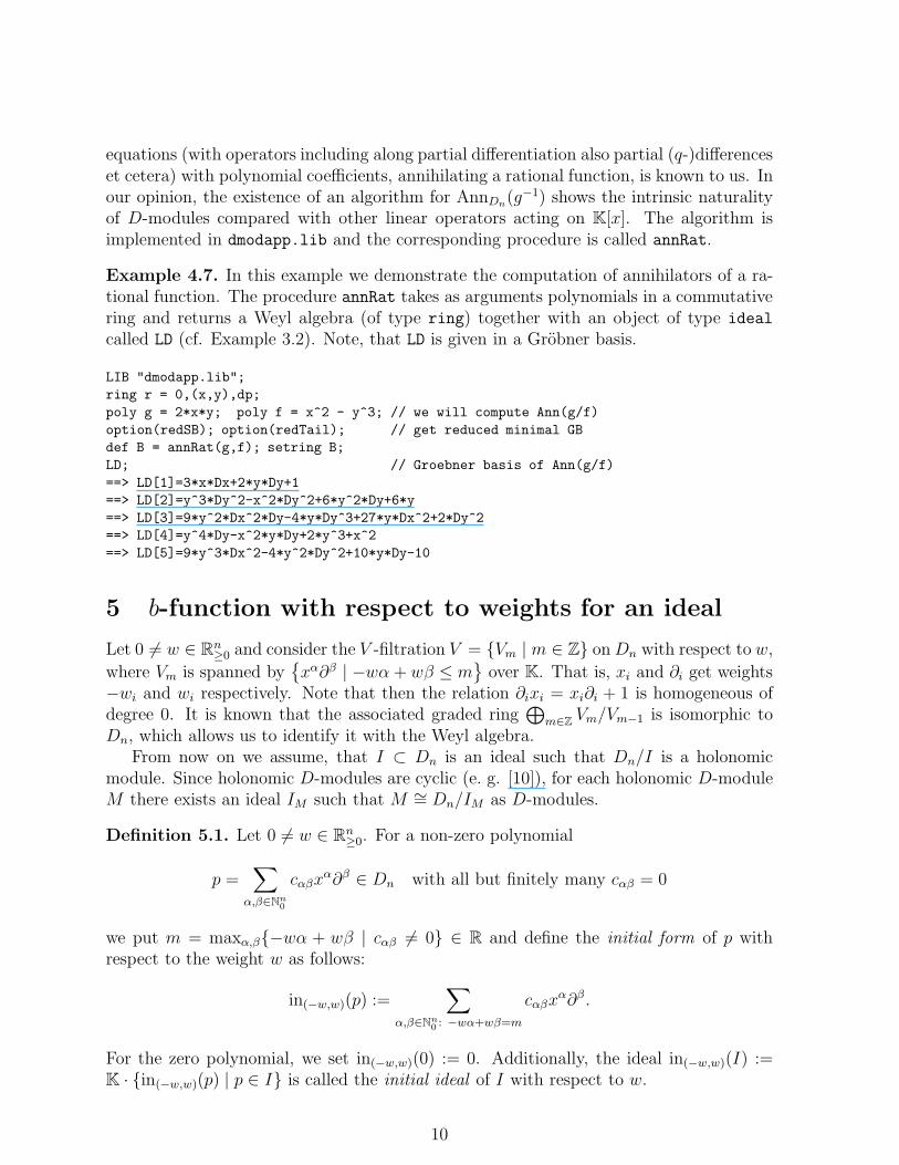
Example 4.7. In this example we demonstrate the computation of annihilators of a ra-tional function. The procedure annRat takes as arguments polynomials in a commutativering and returns a Weyl algebra (of type ring) together with an object of type ideal

called LD (cf. Example 3.2). Note, that LD is given in a Grobner basis.

LIB "dmodapp.lib";

ring r = 0,(x,y),dp;

poly g = 2*x*y; poly f = x^2 - y^3; // we will compute Ann(g/f)

option(redSB); option(redTail); // get reduced minimal GB

def B = annRat(g,f); setring B;

LD; // Groebner basis of Ann(g/f)

==> LD[1]=3*x*Dx+2*y*Dy+1

==> LD[2]=y^3*Dy^2-x^2*Dy^2+6*y^2*Dy+6*y

==> LD[3]=9*y^2*Dx^2*Dy-4*y*Dy^3+27*y*Dx^2+2*Dy^2

==> LD[4]=y^4*Dy-x^2*y*Dy+2*y^3+x^2

==> LD[5]=9*y^3*Dx^2-4*y^2*Dy^2+10*y*Dy-10

5 b-function with respect to weights for an ideal

Let 0 6= w ∈ Rn≥0 and consider the V -filtration V = {Vm | m ∈ Z} onDn with respect to w,

where Vm is spanned by{xα∂β | −wα + wβ ≤ m

}over K. That is, xi and ∂i get weights

−wi and wi respectively. Note that then the relation ∂ixi = xi∂i + 1 is homogeneous ofdegree 0. It is known that the associated graded ring

⊕m∈Z Vm/Vm−1 is isomorphic to

Dn, which allows us to identify it with the Weyl algebra.From now on we assume, that I ⊂ Dn is an ideal such that Dn/I is a holonomic

module. Since holonomic D-modules are cyclic (e. g. [10]), for each holonomic D-moduleM there exists an ideal IM such that M ∼= Dn/IM as D-modules.

Definition 5.1. Let 0 6= w ∈ Rn≥0. For a non-zero polynomial

p =∑

α,β∈Nn0

cαβxα∂β ∈ Dn with all but finitely many cαβ = 0

we put m = maxα,β{−wα + wβ | cαβ 6= 0} ∈ R and define the initial form of p withrespect to the weight w as follows:

in(−w,w)(p) :=∑

α,β∈Nn0 : −wα+wβ=m

cαβxα∂β .

For the zero polynomial, we set in(−w,w)(0) := 0. Additionally, the ideal in(−w,w)(I) :=K · {in(−w,w)(p) | p ∈ I} is called the initial ideal of I with respect to w.

10

Definition 5.2. Let 0 6= w ∈ Rn≥0 and s :=

∑ni=1wixi∂i. Then in(−w,w)(I) ∩ K[s] is a

principal ideal in K[s]. Its monic generator bI,w(s) is called the global b-function of I withrespect to the weight w.

Theorem 5.3. The global b-function is nonzero.

We will give a proof of this well-known result in Section 5.2.Following its definition, the computation of the global b-function of I with respect

to w can be done in two steps:

1. Compute the initial ideal I ′ of I with respect to w.

2. Compute the intersection of I ′ with the subalgebra K[s].

We will discuss both steps separately, starting with the initial ideal. It is importantto mention, that although this procedure has been described in [34], this approach wascompletely treated by Noro in [30], accompanied with a very impressive implementationin Risa/Asir.

5.1 Computing the initial ideal

In order to compute the initial ideal, the method of weighted homogenization is proposedin [30], which we will describe below.

Let u, v ∈ Rn>0. The G-algebra D

(h)(u,v) := K〈x1, . . . , xn, ∂1, . . . , ∂n, h | {xjxi = xixj , ∂j∂i

= ∂i∂j , xih = hxi, ∂ih = h∂i, ∂jxi = xi∂j + δi,jhui+vj}〉 is called the n-th weighted homoge-

nized Weyl algebra with weights u, v, i. e. xi and ∂i get weights ui and vi respectively.For p =

∑α,β cαβx

α∂β ∈ Dn we define the weighted homogenization of p as follows:

H(u,v)(p) =∑

α,β

cαβhdeg(u,v)(p)−(uα+vβ)xα∂β .

This definition naturally extends to a set of polynomials. Here, deg(u,v)(p) denotes theweighted total degree of p with respect to weights u, v for x, ∂ and weight 1 for h.

For a monomial ordering ≺ on Dn, which is not necessarily a well-ordering, we definean associated homogenized global ordering ≺(h) in D

(h)(u,v) by setting h ≺(h) xi, h ≺(h) ∂i

for all i and,

p ≺(h) q if deg(u,v)(p) < deg(u,v)(q)

or deg(u,v)(p) = deg(u,v)(q) and p|h=1≺ q|h=1

.

Note that for u = v = (1, . . . , 1) this is exactly the standard homogenization as in [34]and [9]. Analogue statements of the following two theorems can be found in [34] and [30]respectively.

Theorem 5.4. Let F be a finite subset of Dn and ≺ a global ordering. If G(h) is aGrobner basis of 〈H(u,v)(F )〉 with respect to ≺(h), then G(h)

|h=1is a Grobner basis of 〈F 〉

with respect to ≺.

11

Theorem 5.5. Let ≺ be a global monomial ordering on Dn and ≺(−w,w) the non-globalordering defined by

xα∂β ≺(−w,w) xγ∂δ if −wα + wβ < −wγ + wδ

or −wα + wβ = −wγ + wδ and xα∂β ≺ xγ∂δ.

If G(h) is a Grobner basis of H(u,v)(I) with respect to ≺(h)(−w,w), then the set {in(−w,w,0)(g) |

g ∈ G(h)} is a Grobner basis of in(−w,w,0)(H(u,v)(I)) with respect to ≺(h).

Proof. Let f ′ ∈ in(−w,w,0)(H(u,v)(I)) be (−w,w, 0)-homogeneous. There exist f ∈ H(u,v)(I)and g ∈ G(h) such that f ′ = in(−w,w,0)(f) and lm

≺(h)(−w,w)

(g) | lm≺

(h)(−w,w)

(f). Since f, g are

(u, v)-homogeneous, we have

lm≺

(h)(−w,w)

(g) = lm≺(h)(in(−w,w,0)(g)), lm≺

(h)(−w,w)

(f) = lm≺(h)(in(−w,w,0)(f)),

which concludes the proof.

Summarizing the results from this section, we obtain the following algorithm to com-pute the initial ideal.

Algorithm 5.6 (InitialIdeal). Input: I ⊂ Dn a holonomic ideal, 0 6= w ∈ Rn≥0, ≺ a

global ordering on Dn, u, v ∈ Rn>0

Output: A Grobner basis G of in(−w,w)(I) with respect to ≺

≺(h)(−w,w):= the homogenized ordering as defined in theorem 5.5

G(h) := a Grobner basis of H(u,v)(I) with respect to ≺(h)(−w,w)

return G = in(−w,w)(G(h)

|h=1)

5.2 Intersecting an ideal with a principal subalgebra

We will now consider a much more general setting than needed to compute the globalb-function. Let A be an associative K-algebra. We are interested in computing theintersection of a left ideal J ⊂ A with the subalgebra K[s] of A where s ∈ A is an arbitrarynon-constant element. This intersection is always generated by one element since K[s] isa principal ideal domain. In other words, we want to find the monic generator b ∈ A suchthat 〈b〉 = J ∩K[s].

For this section, we will assume that there is an ordering on A such that there existsa finite left Grobner basis G of J .

Then we can distinguish between the following four situations:

1. No leading monomials of elements in G divide the leading monomial of any powerof s.

2. There is an element in G whose leading monomial divides the leading monomial ofsome power of s. In this situation, we have the following sub-situations.

12

2.1. J · s ⊂ J and dimK(EndA(A/J)) <∞.

2.2. One of the two conditions in 2.1. does not hold.

2.2.1. The intersection is zero.

2.2.2. The intersection is not zero.

Lemma 5.7. If there exists no g ∈ G such that lm(g) divides lm(sk) for some k ∈ N0,then J ∩K[s] = {0}.

The lemma covers the first case above. In the second case however, we cannot ingeneral state whether the intersection is trivial or not as the following example illustrates.

Remark 5.8. The converse of the previous lemma is wrong. For instance, consider K[x, y]and J = 〈y2 + x〉. Then J ∩ K[y] = {0} while {y2 + x} is a Grobner basis of J for anyordering.

In situation 2.1. though, the intersection is not zero as the following lemma shows,inspired by the sketch of the proof of Theorem 5.3 in [34].

Lemma 5.9. Let J · s ⊂ J and dimK(EndA(A/J)) <∞. Then J ∩K[s] 6= {0}.

Proof. Consider the right multiplication with s as a map A/J → A/J which is a well-defined A-module endomorphism of A/J as a− a′ ∈ J implies that (a− a′)s ∈ J · s ⊂ J ,which holds by assumption for all a, a′ ∈ A. Since EndA(A/J) is finite dimensional,linear algebra guarantees that this endomorphism has a well-defined non-zero minimalpolynomial µ. Moreover, µ is precisely the monic generator of J ∩ K[s] as µ(s) = [0] inA/J , hence µ(s) ∈ J ∩K[s], and deg(µ) is minimal by definition.

Remark 5.10. In particular, the lemma holds if A/J itself is a finite dimensional A-module. In the case where A is a Weyl algebra and A/J is a holonomic module, we knowthat dimK(EndA(A/J)) is finite (cf. [34]).

For situation 2.1., we have reduced our problem of intersecting an ideal with a sub-algebra generated by one element to a problem from linear algebra by the proof of thelemma, namely to the one of finding the minimal polynomial of an endomorphism.

Proof of Theorem 5.3. Let 0 6= w ∈ Rn≥0, J := in(−w,w)(I) for a holonomic ideal I ⊂ Dn

and s :=∑n

i=1wixi∂i. Without loss of generality let 0 6= p =∑

α,β cα,βxα∂β ∈ J be

(−w,w)-homogeneous. Then we obtain for every monomial in p by using the Leibniz rule

xα∂βxi∂i = xα+ei∂β+ei + βixα∂β = (∂ix

αi+1i − (αi + 1)xαi

i )xα

xαi

i

∂β + βixα∂β

= (∂ixi − (αi + 1) + βi)xα∂β = (xi∂i − αi + βi)x

α∂β .

Put m = −wα + wβ for some term cα,βxα∂β in p where cα,β is non-zero. Since p is

(−w,w)-homogeneous, m does not depend on the choice of this term. Hence,

p · s = pn∑

i=1

wixi∂i =n∑

i=1

wi

∑

α,β

(xi∂i − αi + βi)cα,βxα∂β

= s · p+n∑

i=1

∑

α,β

wi(−αi + βi)cα,βxα∂β = (s+m) · p ∈ J.

13

Since Dn/J is holonomic (cf. [34]) and J · s ⊂ J , Remark 5.10 and Lemma 5.9 yield theclaim.

If one knows in advance that the intersection is not zero, the following algorithmterminates.

Algorithm 5.11 (principalIntersect).

Input: s ∈ A, J ⊂ A a left ideal such that J ∩K[s] 6= {0}.Output: b ∈ K[s] monic such that J ∩K[s] = 〈b〉G := a finite left Grobner basis of J (assume it exists)i := 1loop

if there exist a0, . . . , ai−1 ∈ K such that NF(si, G) +∑i−1

j=0 aj NF(sj , G) = 0 then

return b := si +∑i−1

j=0 ajsj

else

i := i+ 1end if

end loop

Note that because NF(si, G)+∑i−1

j=0 aj NF(sj , G) = 0 is equivalent to si+

∑i−1j=0 ajs

j ∈J , the algorithm searches for a monic polynomial in K[s] that also lies in J . This is doneby going degree by degree through the powers of s until there is a linear dependency.This approach also ensures the minimality of the degree of the output. The algorithmterminates if and only if J ∩K[s] 6= {0}. Note that this approach works over any field.

The check whether there is a linear dependency over K between the computed normalforms of the powers of s is done by the procedure linReduce in our implementation.

5.2.1 An enhanced computation of normal forms

When computing normal forms of the form NF(si, J) like in algorithm 5.11 we can speedup the reduction process by making use of the previously computed normal forms.

Lemma 5.12. Let A be a K-algebra, J ⊂ A a left ideal and let f ∈ A. For i ∈ N putri = NF(f i, J), qi = f i − ri ∈ J and ci =

lc(qir1)lc(r1qi)

provided r1qi 6= 0. For r1qi = 0 we putci = 0. Then we have for all i ∈ N

ri+1 = NF(fri, J) = NF([f i − ri, r1]ci + rir1, J).

As a consequence, we obtain the following result for some K-algebras of special im-portance.

Corollary 5.13. If A is a G-algebra of Lie type (e. g. a Weyl algebra), then

ri+1 = NF(fri, J) = NF([f i − ri, r1] + rir1, J) holds.

If A is commutative, we have ri+1 = NF(rir1, J) = NF(r1, J)i+1 = NF(ri+1

1 , J).

Note, that computing Lie bracket [f, g] both in theory and in practice is easier andfaster, than to compute [f, g] as f · g − g · f , see e. g. [22].

14

5.2.2 Applications

Apart from computing global b-functions, there are various other applications of Algo-rithm 5.11.

Solving Zero-dimensional Systems. Recall that an ideal I ⊂ K[x1, . . . , xn] is calledzero-dimensional if one of the following equivalent conditions holds:

• K[x1, . . . , xn]/I is finite dimensional as a K-vector space.

• For each 1 ≤ i ≤ n there exist 0 6= fi ∈ I ∩K[xi].

• The cardinality of the zero-set of I is finite.

In order to compute the zero-set of I, one can use the classical triangularizationalgorithms. These algorithms require to compute a Grobner basis with respect to someelimination ordering (like lexicographic one), which might be very hard.

By Algorithm 5.11, a generator of I ∩K[xi] can be computed without these expensiveorderings. Instead, any ordering, hence a better suited one, may be freely chosen.

A similar approach is used in the celebrated FGLM algorithm (cf. [12]).

Computing Central Characters and Algebraic Dependence. Let A be an asso-ciative K-algebra. Intersection of a left ideal with the center of A, which is isomorphic toa commutative ring, is important for many algorithms, among other for the computationof central character decomposition of a finitely presented module (cf. [19] for the theoryand [1] for an example with Principal Intersection). In the situation, where the centerof A is generated by one element (which is not seldom), we can apply Algorithm 5.11to compute the intersection (known to be often quite nontrivial) without engaging muchmore expensive Grobner basis computation, which use elimination.

Example 5.14. Consider the quantum algebra U ′q(so3) (as defined by Fairlie and Odesskii)

for q2 being the n-th root of unity. It is known, that then, in addition to the single gen-erator C of the center present over any field, three new elements Zi, depending on n willappear. Since U ′

q(so3) has Gel’fand-Kirillov dimension 3, four commuting elements in itobey a single polynomial algebraic dependency (the ideal of dependencies in principal).Computing such a dependency is a very tough challenge for Grobner bases. But as wesee, it is quite natural to apply Principal Intersection.

LIB "ncalg.lib"; LIB "bfun.lib";

def A = makeQso3(5); // below Q^2 is the 5th root of unity

setring A;

// central elements, depending on Q in their classical form:

ideal I = x5+(Q3-Q2+2)*x3+(Q3-Q2+1)*x, y5+(Q3-Q2+2)*y3+(Q3-Q2+1)*y,

z5+(Q3-Q2+2)*z3+(Q3-Q2+1)*z;

I = twostd(I); // two-sided Groebner basis

poly C = 5*xyz+(4Q3-3Q2+2Q-1)*x2+(-Q3+2Q2-3Q+4)*y2+(4Q3-3Q2+2Q-1)*z2;

poly v = vec2poly(pIntersect(C,I),1); // present vector as poly

poly t = subst(v,x,C); t; // t as a polynomial in C of size 42

==> 3125*x5y5z5+(3125Q3-3125Q2+6250)*x5y5z3+(3125Q3-3125Q2+6250)*x5y3z5+ ...

15

// present matrix of cofactors of t as an element of I:

matrix T = lift(I,t);

poly a = 125*(25*I[1]*I[2]*I[3]+(Q3-7Q2+8Q-4)*(I[1]^2+I[2]^2+I[3]^2));

a-t; // a expresses t in the subalgebra gen. by I[1..3]

==> 0

// define univariate ring over algebraic extension:

ring r = (0,Q),c,dp; minpoly = Q4-Q3+Q2-Q+1;

poly v = fetch(A,v); // map v from A to a univariate poly in c

factorize(v);

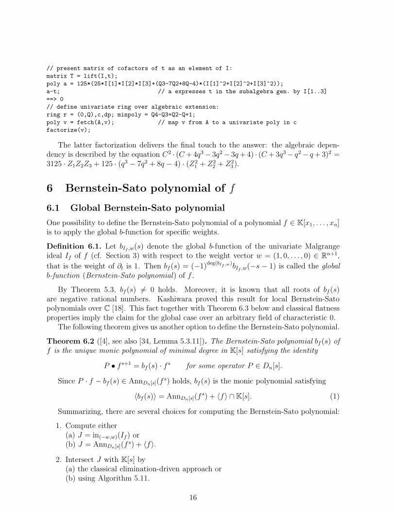
The latter factorization delivers the final touch to the answer: the algebraic depen-dency is described by the equation C2 · (C +4q3− 3q2− 3q+4) · (C +3q3− q2− q+3)2 =3125 · Z1Z2Z3 + 125 · (q3 − 7q2 + 8q − 4) · (Z2

1 + Z22 + Z2

3 ).

6 Bernstein-Sato polynomial of f

6.1 Global Bernstein-Sato polynomial

One possibility to define the Bernstein-Sato polynomial of a polynomial f ∈ K[x1, . . . , xn]is to apply the global b-function for specific weights.

Definition 6.1. Let bIf ,w(s) denote the global b-function of the univariate Malgrangeideal If of f (cf. Section 3) with respect to the weight vector w = (1, 0, . . . , 0) ∈ Rn+1,

that is the weight of ∂t is 1. Then bf (s) = (−1)deg(bIf ,w)bIf ,w(−s − 1) is called the globalb-function (Bernstein-Sato polynomial) of f .

By Theorem 5.3, bf(s) 6= 0 holds. Moreover, it is known that all roots of bf (s)are negative rational numbers. Kashiwara proved this result for local Bernstein-Satopolynomials over C [18]. This fact together with Theorem 6.3 below and classical flatnessproperties imply the claim for the global case over an arbitrary field of characteristic 0.

The following theorem gives us another option to define the Bernstein-Sato polynomial.

Theorem 6.2 ([4], see also [34, Lemma 5.3.11]). The Bernstein-Sato polynomial bf (s) off is the unique monic polynomial of minimal degree in K[s] satisfying the identity

P • f s+1 = bf (s) · fs for some operator P ∈ Dn[s].

Since P · f − bf (s) ∈ AnnDn[s](fs) holds, bf (s) is the monic polynomial satisfying

〈bf(s)〉 = AnnDn[s](fs) + 〈f〉 ∩K[s]. (1)

Summarizing, there are several choices for computing the Bernstein-Sato polynomial:

1. Compute either(a) J = in(−w,w)(If) or(b) J = AnnDn[s](f

s) + 〈f〉.

2. Intersect J with K[s] by(a) the classical elimination-driven approach or(b) using Algorithm 5.11.

16

It is very interesting to investigate the approach for the computation of Bernstein-Satopolynomial, which arises as the combination of the two methods:

1. AnnDn[s](fs) via Briancon-Maisonobe (cf. [20]),

2. (Ann(Dn[s]fs) + 〈f〉) ∩K[s] via Algorithm 5.11.

For an efficient computation of in(−w,w)(If) using the method of weighted homog-enization as described in Section 5.1, Noro proposes [30] to choose the weights u =(degu(f), u1, . . . , un), v = (1, degu(f)−u1+1, . . . , degu(f)−un+1), such that the weightof t is degu(f) and the weight of ∂t is 1. Here, u ∈ Rn

>0 is an arbitrary vector and degu(f)denotes the weighted total degree of f with respect to u. The vector u may be chosenheuristically in accordance to the shape of f or by default, one can set u = (1, . . . , 1).

6.2 Implementation

For the computation of Bernstein-Sato polynomials, we offer the following procedures inthe Singular library bfun.lib:

bfct computes in(−w,w)(If) using weighted homogenization with weights u, v for anoptional weight vector u (by default u = (1, . . . , 1)) as described above, and then uses Al-gorithm 5.11, where the occurring systems of linear equations are solved by the procedurelinReduce.

bfctAnn computes AnnDn[s](fs) via Briancon-Maisonobe and intersects AnnDn[s](f

s)+〈f〉 with K[s] analogously to bfct.

bfctOneGB computes the initial ideal and the intersection at once using a homogenizedelimination ordering, a similar approach has been used in [16].

For the global b-function of an ideal I ⊂ Dn, bfctIdeal computes in(−w,w)(I) usingstandard homogenization, i. e. weighted homogenization where all weights are equal to 1,and then proceeds the same way as bfct. Recall that Dn/I must be holonomic as in [34].

All these procedures work as the following example illustrates for bfct and the hyper-plane arrangement xyz(z − y)(y + z).

LIB "bfun.lib";

ring r = 0,(x,y,z),dp; // commutative ring

poly f = x*y*z*(z-y)*(y+z);

list L = bfct(f);

print(matrix(L[1])); // the roots of the BS-polynomial

==> -1,-5/4,-3/4,-3/2,-1/2

L[2]; // the multiplicities of the roots above

==> 3,1,1,1,1

6.3 Local Bernstein-Sato Polynomial

Here we are interested in what kind of information one can obtain from the local b-functions for computing the global one and conversely. In order to avoid theoreticalproblems we will assume in this paragraph that the ground field K = C.

Several algorithms to obtain the local b-function of a hypersurface f have been knownwithout any Grobner bases computation but under some conditions on f . For instance,

17

it was shown by Malgrange [24] that the minimal polynomial of −∂tt acting on somevector space of finite dimension coincides with the reduced (local) Bernstein polynomial,assuming that the singularity is isolated.

The algorithms of Oaku [32] used Grobner bases for the first time. Recently, Nakayamapresented some algorithms, which use the global b-function as a bound and obtain a localb-function by Mora resp. approximate division [27], see also the work of Nishiyama andNoro [29].

Theorem 6.3 (Briancon-Maisonobe (unpublished), Mebkhout-Narvaez [26]). Let bf,P (s)be the local b-function of f at the point P ∈ Cn and bf (s) the global one. Then it is ver-ified that bf(s) = lcmP∈Cn bf,P (s) = lcmP∈Σ(f) bf,P (s), where Σ(f) = V (〈f, ∂f

∂x1, . . . , ∂f

∂xn〉)

denotes the singular locus of V (f).

Remark 6.4. Assume, that Σ(f) consists of finitely many isolated singular points (thedimension of the corresponding defining ideal is 0). Then the computation of the globalb-function with Theorem 6.3 becomes effective. Moreover, one needs just an algorithmfor computing the local b-function of a hypersurface, having an isolated singularity at theorigin.

The Singular library gmssing.lib, developed and implemented by M. Schulze [36],contains the procedure bernstein, which computes the local b-function at the origin. Itreturns the list of roots and corresponding multiplicities.

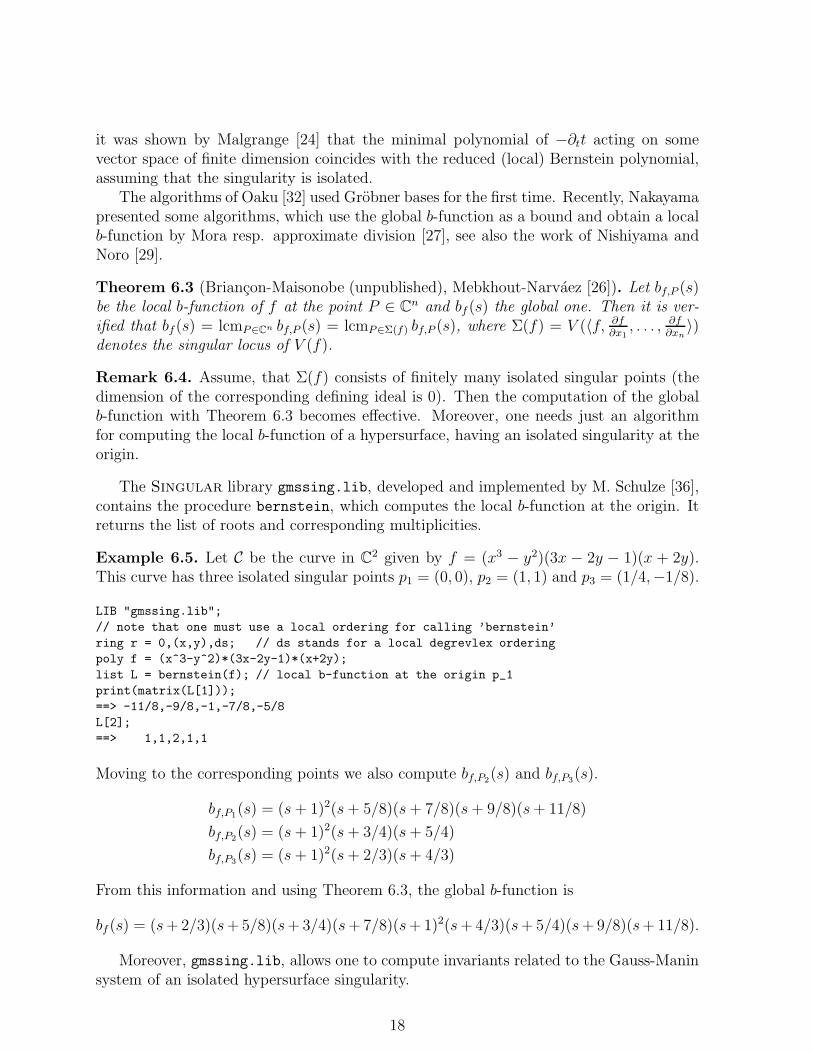
Example 6.5. Let C be the curve in C2 given by f = (x3 − y2)(3x − 2y − 1)(x + 2y).This curve has three isolated singular points p1 = (0, 0), p2 = (1, 1) and p3 = (1/4,−1/8).

LIB "gmssing.lib";

// note that one must use a local ordering for calling ’bernstein’

ring r = 0,(x,y),ds; // ds stands for a local degrevlex ordering

poly f = (x^3-y^2)*(3x-2y-1)*(x+2y);

list L = bernstein(f); // local b-function at the origin p_1

print(matrix(L[1]));

==> -11/8,-9/8,-1,-7/8,-5/8

L[2];

==> 1,1,2,1,1

Moving to the corresponding points we also compute bf,P2(s) and bf,P3(s).

bf,P1(s) = (s+ 1)2(s+ 5/8)(s+ 7/8)(s+ 9/8)(s+ 11/8)

bf,P2(s) = (s+ 1)2(s+ 3/4)(s+ 5/4)

bf,P3(s) = (s+ 1)2(s+ 2/3)(s+ 4/3)

From this information and using Theorem 6.3, the global b-function is

bf (s) = (s+2/3)(s+5/8)(s+3/4)(s+7/8)(s+1)2(s+4/3)(s+5/4)(s+9/8)(s+11/8).

Moreover, gmssing.lib, allows one to compute invariants related to the Gauss-Maninsystem of an isolated hypersurface singularity.

18

In the non-isolated case the situation is more complicated. For computing the local b-function in this case (which is important on its own) we suggest using two methods: Takethe global b-function as an upper bound and a local version of the checkRoot algorithm,see below. Another method is to use a local version of principalIntersect, which isunder development. Despite the existence of many algorithms, the effectiveness of thecomputation of local b-functions is still to be drastically enhanced.

6.4 Partial knowledge of Bernstein-Sato polynomial

As we have mentioned, several algorithms for computing the b-function associated witha polynomial have been known. However, in general it is very hard from computationalpoint of view to obtain this polynomial, and in the actual computation a limited numberof examples can be treated. For some applications only the integral roots of bf (s) areneeded and that is why we are interested in obtaining just a part of the Bernstein-Satopolynomial.

Recall the algorithm checkRoot for checking whether a rational number is a root ofthe b-function of a hypersurface from [20]. Equation (1) was used to prove the followingresult.

Theorem 6.6. ([20]) Let R be a ring whose center contains K[s] as a subring. Letus consider q(s) ∈ K[s] a polynomial in one variable and I a left ideal in R satisfyingI ∩K[s] 6= 0. Then (I + R〈q(s)〉) ∩K[s] = I ∩K[s] +K[s]〈q(s)〉. In particular, using theabove equation (1), we have

(AnnDn[s](f

s) +Dn[s] · 〈f, q(s)〉)∩K[s] = 〈bf(s), q(s)〉.

As a consequence, let mα be the multiplicity of α as a root of bf (−s) and let us considerthe ideals Ji = AnnDn[s](f

s) + 〈f, (s + α)i+1〉 ⊆ Dn[s], i = 0, . . . , n, then [mα > i ⇐⇒(s+ α)i /∈ Ji ].

Once we know a system of generators of the annihilator of f s in Dn[s], the last theoremprovides an algorithm for checking whether a given rational number is a root of the b-function of f and for computing its multiplicity, using Grobner bases for differentialoperators.

This algorithm is much faster, than the computation of the whole Bernstein polynomialvia Grobner bases, because no elimination ordering is needed for computing a Grobnerbasis of Ji, once one knows a system of generators of AnnDn[s](f

s). Also, the element(s + α)i+1, added as a generator, seems to simplify tremendously such a computation.Actually, when i = 0 it is possible to eliminate the variable s in advance and we canperform the whole computation in Dn. Let us see an example.

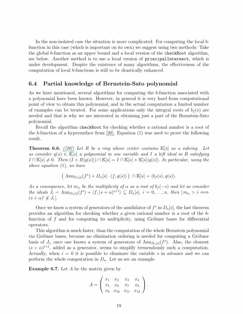
Example 6.7. Let A be the matrix given by

A =

x1 x2 x3 x4x5 x6 x7 x8x9 x10 x11 x12

.

19

Let us denote by ∆i, i = 1, 2, 3, 4, the determinant of the minor resulting from deleting thei-th column of A, and consider f = ∆1∆2∆3∆4. The polynomial f defines a non-isolatedhypersurface in C12. Therefore, from [33] (see also [41]), the set of all possible integral roots

of bf (−s) is {11, 10, 9, 8, 7, 6, 5, 4, 3, 2, 1}. It is known that AnnDn[s](fs) = Ann

(1)Dn[s]

(f s)

(see Section 8) and this fact can be used to simplify the computation of the annihilator.

LIB "dmod.lib";

ring R = 0,(x1,x2,x3,x4,x5,x6,x7,x8,x9,x10,x11,x12),dp;

matrix A[3][4] = x1,x2,x3,x4, x5,x6,x7,x8, x9,x10,x11,x12;

poly Delta1 = det(submat(A,1..3,intvec(2,3,4)));

... // analogous for Delta2 ... Delta4

poly f = Delta1*Delta2*Delta3*Delta4;

def D = Sannfslog(f); setring D; // logarithmic annihilator

poly f = imap(R,f); number alpha = 11;

checkRoot1(LD1,f,alpha);

==> 0

Using the algorithm checkRoot we have proved that the minimal integral root of bf (s)is −1. This example was suggested by F. Castro-Jimenez and J. M. Ucha for testing theLogarithmic Comparison Theorem. A nice introduction to this topic can be found, forinstance, in [39].

Let g be the polynomial resulting from f by substituting x1, x2, x3, x4, x5, x9 with 1.One can show that bg(s) divides bf (s) (see [21] for details). Using the checkRoot algorithmwe have found that (s + 1)4(s + 1/2)(s + 3/2)(s + 3/4)(s + 5/4) is a factor of bg(s) andtherefore a factor of bf (s).

Remark 6.8. Using the notation from Section 5, given a holonomic D-module D/I,it is verified that (in(−w,w)(I) + 〈q(s)〉) ∩ K[s] = 〈bI,w(s), q(s)〉, although Theorem 6.6cannot be applied, since s =

∑wixi∂i does not commute with all operators. For some

applications like integration and restriction the maximal and the minimal integral rootof the b-function of I with respect to some weight vector have to be computed, see [34].However, the above formula cannot be used to find the set of all integral roots, since noupper/lower bound exists in advance. For instance, as it was suggested by N. Takayama,I = 〈t∂t+ k〉, k ∈ Z is D1-holonomic and one has in(−1,1)(I)∩C[s] = 〈s+ k〉 with s = t∂t.

We close this section by mentioning that there exist some well-known methods toobtain an upper bound for the Bernstein-Sato polynomial of a hypersurface singularityonce we know, for instance, an embedded resolution of such singularity [18]. Thereforeusing this result by Kashiwara and the checkRoot algorithm, it is possible to computethe whole Bernstein-Sato polynomial without elimination orderings, see Example 1 in[20]. We investigate different methods in conjunction with the further development of thecheckRoot family of algorithms in [21].

7 Bernstein operator of f

We define the Bernstein-Sato polynomial bf (s) to be the monic generator of a principalideal, hence it is unique. But the so-called B-operator P (s) ∈ Dn[s] from Theorem 6.2 isnot unique.

20

Proposition 7.1. Let G be a left Grobner basis of AnnDn[s](fs+1) and define a Bernstein

operator to be the result of the reduced normal form NF(P (s), G) of some B-operatorP (s). Then, for a fixed monomial ordering on Dn[s], the Bernstein operator is uniquelydetermined.

Proof. Suppose that there is another Q(s) ∈ Dn[s], such that the identities

P (s)f s+1 = bf (s)fs and Q(s)f s+1 = bf (s)f

s hold in the module Dn[s]/AnnDn[s](fs).

Then (P (s) − Q(s))f s+1 = 0, that is P (s) − Q(s) ∈ AnnDn[s](fs+1). Hence, the set

{R(s) ∈ Dn[s] | R(s)f s+1 = bf (s)fs} can be viewed as an equivalence class and we

can take the reduced normal form of any such operator (with respect to G) to be thecanonical representative of the class. Since the reduced normal form with respect to afixed monomial ordering on Dn[s] is unique, so is the Bernstein operator NF(R(s), G).

Note, that we can obtain the left Grobner basis of AnnDn[s](fs+1) via substituting s

with s+ 1 in the left Grobner basis of AnnDn[s](fs).

One can compute the Bernstein operator from the knowledge of AnnDn[s](fs) and bf (s)

by the following methods.

7.1 B-operator via lifting

The algorithm Lift(F,G) computes the transformation matrix, expressing the set ofpolynomials G via the set F , provided 〈G〉 ⊆ 〈F 〉. It is a classical application of Grobnerbases.

Lemma 7.2. Suppose, that AnnDn[s](fs) is generated by h1, . . . , hm and bf (s) is known.

The output of Lift({f, h1, . . . , hm}, {bf (s)}) is the 1 × (m + 1) matrix (a, b1, . . . , bm).Then a B-operator is computed as P (s) = NF(a,AnnDn[s](f

s)).

Proof. Because of Equation (1), if (a, b1, . . . , bm) is the output of Lift as in the statement,

bf(s) = af +m∑

i=1

bihi holds,

hence the first element of such a matrix is a B-operator. Thus, the Bernstein operator isobtained via NF(a,AnnDn[s](f

s+1)).

However, we have to mention, that the Lift procedure is quite expensive in general.Note that another method for the computation of a B-operator using lifting techniques

is given by applying Algorithm 8 of [29] with a(x) = 1.

7.2 B-operator via kernel of module homomorphism

1. Consider the Dn[s]-module homomorphism

ϕ : Dn[s] −→ Dn[s]/(AnnDn[s](fs) + 〈bf(s)〉), 1 7→ f,

21

then for u ∈ kerϕ, uf ∈ AnnDn[s](fs) + 〈bf (s)〉. That is, there exist a, bi ∈ Dn[s], such

that

uf = abf (s) +

m∑

i=1

bihi,

However, we are interested in such u, that a ∈ K. This is possible, but the 2nd methodabove proposes a more elegant solution. Also one has to say, that in this case we haveto compute a Grobner basis of AnnDn[s](f

s) + 〈bf (s)〉 as an intermediate step and alsothe kernel of a module homomorphism with respect to the latter. This combination is,in general, quite nontrivial to compute. In the Grobner basis computation a monomialordering, preferring x, ∂x over s seems to be better because of numerous applications ofthe Product Criterion.

2. Consider the Dn[s]-module homomorphism

ϑ : Dn[s]2 −→ Dn[s]/AnnDn[s](f

s), ǫ1 7→ bf (s), ǫ2 7→ f.

Then kerϑ = {(u, v)T ∈ Dn[s]2 | ubf(s) + vf ∈ AnnDn[s](f

s)} is a submodule of Dn[s]2.

Indeed, kerϑ has many generators. In order to get a vector of the form (k, u(s)) for k ∈ K,we perform another Grobner basis computation for a submodule with respect to a modulemonomial ordering, giving preference to the first component over the second one. Sincein the reduced basis there is a single element of the form (k, v(s)) ⊂ kerϑ with k 6= 0, itfollows that P (s) = v(s)k−1.

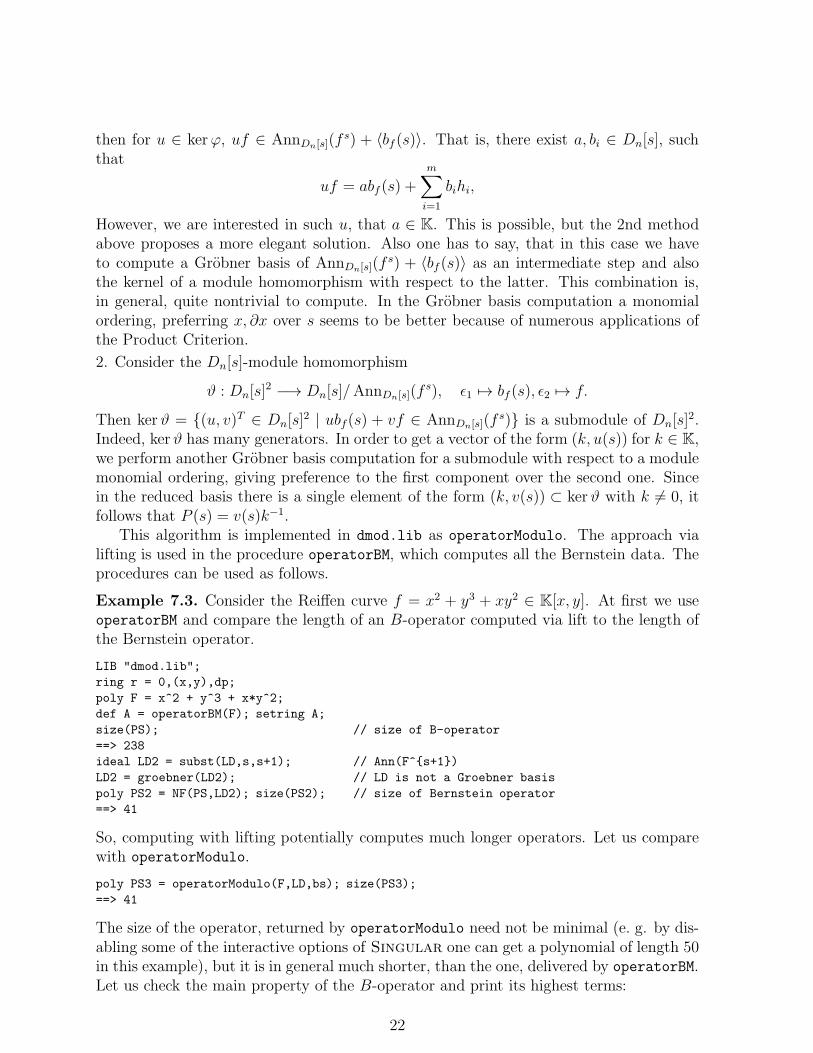
This algorithm is implemented in dmod.lib as operatorModulo. The approach vialifting is used in the procedure operatorBM, which computes all the Bernstein data. Theprocedures can be used as follows.

Example 7.3. Consider the Reiffen curve f = x2 + y3 + xy2 ∈ K[x, y]. At first we useoperatorBM and compare the length of an B-operator computed via lift to the length ofthe Bernstein operator.

LIB "dmod.lib";

ring r = 0,(x,y),dp;

poly F = x^2 + y^3 + x*y^2;

def A = operatorBM(F); setring A;

size(PS); // size of B-operator

==> 238

ideal LD2 = subst(LD,s,s+1); // Ann(F^{s+1})

LD2 = groebner(LD2); // LD is not a Groebner basis

poly PS2 = NF(PS,LD2); size(PS2); // size of Bernstein operator

==> 41

So, computing with lifting potentially computes much longer operators. Let us comparewith operatorModulo.

poly PS3 = operatorModulo(F,LD,bs); size(PS3);

==> 41

The size of the operator, returned by operatorModulo need not be minimal (e. g. by dis-abling some of the interactive options of Singular one can get a polynomial of length 50in this example), but it is in general much shorter, than the one, delivered by operatorBM.Let us check the main property of the B-operator and print its highest terms:

22

NF(PS3*F - bs, subst(LD2,s,s-1));

==> 0

108*PS2; // i.e. the Bernstein operator

==> 6*x*Dx^2*Dy+9*y*Dx^2*Dy-2*x*Dx*Dy^2-4*y*Dx*Dy^2-y*Dy^3+ ...

In the last line we see the terms of highest degree with respect to ∂x, ∂y.

7.3 Grobner free method

As a consequence of Theorem 6.2, one obtains that P · f − bf(s) ∈ AnnDn[s](fs) and

P, bf(s) /∈ AnnDn[s](fs). If we fix an ordering such that bf(s) = NF(bf (s),AnnDn[s](f

s))holds, we may rewrite this relation to bf (s) = NF(P · f,AnnDn[s](f

s)). Hence, we cancompute P by searching for a linear combination of monomials m ∈ Dn[s] that satisfy thisequality when multiplied with f from the right side. Using the results from the beginningof this section, one only needs to consider monomials which span Dn/AnnDn[s](f

s+1) asK-vector space. We get the following algorithm.

Algorithm 7.4.

Input: f ∈ K[x1, . . . , xn], the Bernstein-Sato polynomial bf (s) of fOutput: P ∈ Dn[s], the Bernstein operator of fd := 0loop

Md := {m ∈ Dn[s] | m monomial, deg(m) ≤ d, lm(p) ∤ m ∀ p ∈ AnnDn[s](fs+1)}

if there exist am ∈ K such that bf (s) =∑

m∈MdamNF(m · f,AnnDn[s](f

s)) thenreturn P :=

∑m∈Md

amm− bf (s)

else

d := d+ 1end if

end loop

The search for the coefficients am can be done using linReduce (cf. Algorithm 5.11)as one is in fact looking for a linear dependency between the Bernstein-Sato polynomialand the elements m · f in the vector space Dn[s]/AnnDn[s](f

s).

Remark 7.5. Note, that Algorithm 7.4 can be extended to one searching for both B-operator and Bernstein-Sato polynomial simultaneously. We have to mention, that bothalgorithms of this kind are well suited for the search of operators and Bernstein-Satopolynomials in the case, when both of them are of relatively low total degree.

7.4 Computing integrals and zeta functions

Given a simplex C ⊂ Kn (for K = R,C) and f ∈ K[x1, . . . , xn], we can define ζ(s) :=∫Cf(x)sdx. Since P (s) • f s+1 = bf (s)f

s, we obtain

ζ(s) =

∫

C

f(x)sdx =1

bf (s)

∫

C

P (s) • f(x)s+1dx

23

expanding the latter with e. g. the chain rule, we come to an in general inhomogeneousrecurrence relation for ζ(s), which involves coefficients in K[s]. Since P (s) is globallydefined (and is, of course, independent on C), one can obtain a generic formula for allintegrals of this type.

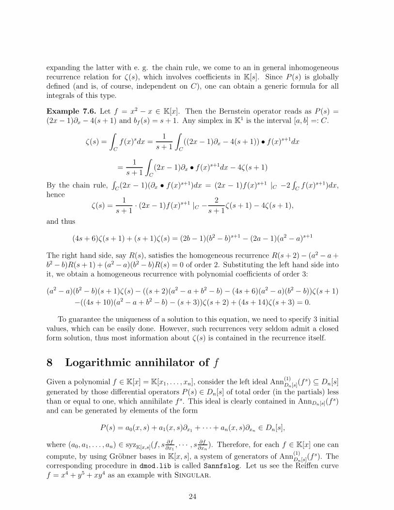
Example 7.6. Let f = x2 − x ∈ K[x]. Then the Bernstein operator reads as P (s) =(2x− 1)∂x − 4(s+ 1) and bf (s) = s+ 1. Any simplex in K1 is the interval [a, b] =: C.

ζ(s) =

∫

C

f(x)sdx =1

s+ 1

∫

C

((2x− 1)∂x − 4(s+ 1)) • f(x)s+1dx

=1

s + 1

∫

C

(2x− 1)∂x • f(x)s+1dx− 4ζ(s+ 1)

By the chain rule,∫C(2x − 1)(∂x • f(x)s+1)dx = (2x − 1)f(x)s+1 |C −2

∫Cf(x)s+1)dx,

hence

ζ(s) =1

s + 1· (2x− 1)f(x)s+1 |C −

2

s + 1ζ(s+ 1)− 4ζ(s+ 1),

and thus

(4s+ 6)ζ(s+ 1) + (s+ 1)ζ(s) = (2b− 1)(b2 − b)s+1 − (2a− 1)(a2 − a)s+1

The right hand side, say R(s), satisfies the homogeneous recurrence R(s+ 2)− (a2 − a+b2 − b)R(s+ 1)+ (a2 − a)(b2 − b)R(s) = 0 of order 2. Substituting the left hand side intoit, we obtain a homogeneous recurrence with polynomial coefficients of order 3:

(a2 − a)(b2 − b)(s + 1)ζ(s)− ((s+ 2)(a2 − a+ b2 − b)− (4s+ 6)(a2 − a)(b2 − b))ζ(s+ 1)

−((4s + 10)(a2 − a + b2 − b)− (s+ 3))ζ(s+ 2) + (4s+ 14)ζ(s+ 3) = 0.

To guarantee the uniqueness of a solution to this equation, we need to specify 3 initialvalues, which can be easily done. However, such recurrences very seldom admit a closedform solution, thus most information about ζ(s) is contained in the recurrence itself.

8 Logarithmic annihilator of f

Given a polynomial f ∈ K[x] = K[x1, . . . , xn], consider the left ideal Ann(1)Dn[s]

(f s) ⊆ Dn[s]

generated by those differential operators P (s) ∈ Dn[s] of total order (in the partials) lessthan or equal to one, which annihilate f s. This ideal is clearly contained in AnnDn[s](f

s)and can be generated by elements of the form

P (s) = a0(x, s) + a1(x, s)∂x1 + · · ·+ an(x, s)∂xn∈ Dn[s],

where (a0, a1, . . . , an) ∈ syzK[x,s](f, s∂f

∂x1, · · · , s ∂f

∂xn). Therefore, for each f ∈ K[x] one can

compute, by using Grobner bases in K[x, s], a system of generators of Ann(1)Dn[s]

(f s). Thecorresponding procedure in dmod.lib is called Sannfslog. Let us see the Reiffen curvef = x4 + y5 + xy4 as an example with Singular.

24

LIB "dmod.lib";

ring R = 0,(x,y),dp;

poly f = x^4+y^5+x*y^4;

def A = Sannfslog(f); setring A; LD1;

==> LD1[1]=4*x^2*Dx+5*x*Dx*y+3*x*y*Dy-16*x*s+4*y^2*Dy-20*y*s

==> LD1[2]=16*x*Dx*y^2-125*x*Dx*y-4*x^2*Dy+4*Dx*y^3+5*x*y*Dy+12*y^3*Dy-100*y^2*Dy

-64*y^2*s+500*y*s

// now we compute the whole annihilator with Sannfs and compare

setring R; def B = Sannfs(f); setring B;

map F = A,x,Dx,y,Dy,s;

ideal LD1 = F(LD1);

LD1 = groebner(LD1);

simplify( NF(LD,LD1), 2);

==> _[1]=36*y^3*Dx^2-36*y^3*Dx*Dy+1125/4*x*y*Dx^2-315/4*x*y*Dx*Dy+ ...

And the latter polynomial is not an element of Ann(1)Dn[s]

(f s) but of Ann(2)Dn[s]

(f s) =

AnnDn[s](fs).

8.1 The annihilator up to degree k

More generally, for a given k ≥ 1 one can consider the left ideal Ann(k)Dn[s]

(f s) ⊆ Dn[s]

generated by the differential operators P (s) ∈ Dn[s] of total order less than or equal tok, such that P (s) annihilate f s. The tower of ideals

Ann(1)Dn[s]

(f s) ( · · · ( Ann(k0)Dn[s]

(f s) = AnnDn[s](fs)

has been recently studied by Narvaez in [28]. It is an open problem to find the minimalinteger k0 satisfying the above condition without computing the whole annihilator.

Computationally the annihilator up to degree k can be obtained using Grobner basesin K[x, s] as follows. Consider P (s) =

∑|β|≤k aβ∂

β ∈ Ann(k)Dn[s]

(f s) and let gβ(x, s) ∈

K[x, s] be the polynomial defined by the formula ∂β · f s = gβ · f s−|β|. Then (aβ)|β|≤k ∈syz(gβf

k−|β|)|β|≤k. Eventually, the polynomials gβ(x, s) can be computed using the ex-pression given in Lemma 8.1.

Given β = (β1, . . . , βn) ∈ Nn, as usual |β| = β1 + · · · + βn, β! = β1! · · ·βn! and∆β

x = 1β!∂βx . A partition of β is a way of writing β as a sum of integral vectors with

non-negative entries. Two sums which only differ in the order of their summands areconsidered to be the same partition. If β = σ1 + . . . + σk with σi 6= 0, then σ is said tobe a partition of length k. The set of all partitions of β (resp. of length k) is denoted by

P(β) (resp. P(β; k)). Obviously P(β) = ∪|β|k=1P(β; k). Finally, we write ℓ(σ) := (ℓστ )τ ,

where ℓστ is the number of times that τ appears in σ.

Lemma 8.1. Using the above notation for all non-zero β ∈ Nn we have,

∆βx · f

s =

|β|∑

k=1

(s

k

) ∑

σ∈P(β;k)

1

ℓ(σ)!∆σ1

x (f) · · ·∆σkx (f) · f s−k .

25

This formula was suggested by Narvaez and can be proved by induction on |β|. Similarexpressions appear in [26, Prop. 5.3.5] and [25, Prop. 2.3.2].

However, despite this almost closed form, the set of polynomials, between which wehave to compute syzygies, is growing fast and the size of polynomials increases. Thisresults in quite hard computations even with the mentioned enhancements.

9 Bernstein-Sato ideals for f = f1 · . . . · fm

Using the results from [13], which we confirmed through intensive testing (cf. [20]),it follows, that the method by Briancon-Maisonobe is the most effective one for thecomputation of s-parametric annihilators where f = f1. Because of the structure ofannihilators in the situation f = f1 · · · fp, p > 1, basically the same principles standbehind the corresponding algorithms. Hence, we decided to implement only Briancon-Maisonobe’s method for the s-parametric annihilator AnnDn[s](f

s) ⊂ Dn[s], where s =(s1, . . . , sp). The corresponding procedure in dmod.lib is called annfsBMI. It computesboth AnnDn[s] f

s ⊂ Dn[s] and the Bernstein-Sato ideal in K[s], which is defined as

B(f) = (AnnDn[s1,...,sp](fs11 · · · f sp

p ) + 〈f1 · · ·fp〉) ∩K[s1, . . . , sp].

In contrary to the case f = f1, in general the ideal B(f) need not be principal. How-ever, it is an open question to give a criterion for the principality of B(f). Armed withsuch a criterion, one can apply a generalization of the method of Principal Intersection5.11 to multivariate subalgebras [2] and thus replace expensive elimination above by thecomputation of a minimal polynomial. Otherwise we still can apply the Principal Inter-section, which, however, will deliver only one polynomial to us. As in the case f = f1 it isan open question, which strategy and which orderings should one use in the computationof the annihilator and of the Bernstein-Sato ideal in order to achieve better performance.

We reported in [20] on several challenges, which have been solved with the help of ourimplementation. Namely, the products (x3 + y2)(x2 + y3) and (x2 + y2+ y3)(x3 + y2) giverise to principal Bernstein-Sato ideals.

Example 9.1. Let us consider the following example from [3], which is quite challengingto compute indeed.

LIB "dmod.lib"; ring r = 0,(x,y,z),dp;

ideal F = z, x^5 + y^5 + x^2*y^3*z;

def A = annfsBMI(F); setring A;

LD; // prints the annihilator in D[s1,s2]

BS; // prints the Bernstein-Sato ideal

We do not show the output here because of its size. But from the output one can see,the Bernstein-Sato ideal is of dimension 1 in D3[s1, s2] since its Grobner basis consistsof three elements {15625s1s

82 +17 l.o.t., 3125s21s

72 +24 l.o.t., 625s51s

62 +42 l.o.t.}. Notably,

every generator factorizes into linear factors and each factor involves either s1 or s2, whichhappens quite seldom in general.

In general, quite a little is known about Bernstein-Sato ideals. Their dimensions, prin-cipality, factorization of generators and primary decomposition constitute open problemsfrom the theoretical side.

26

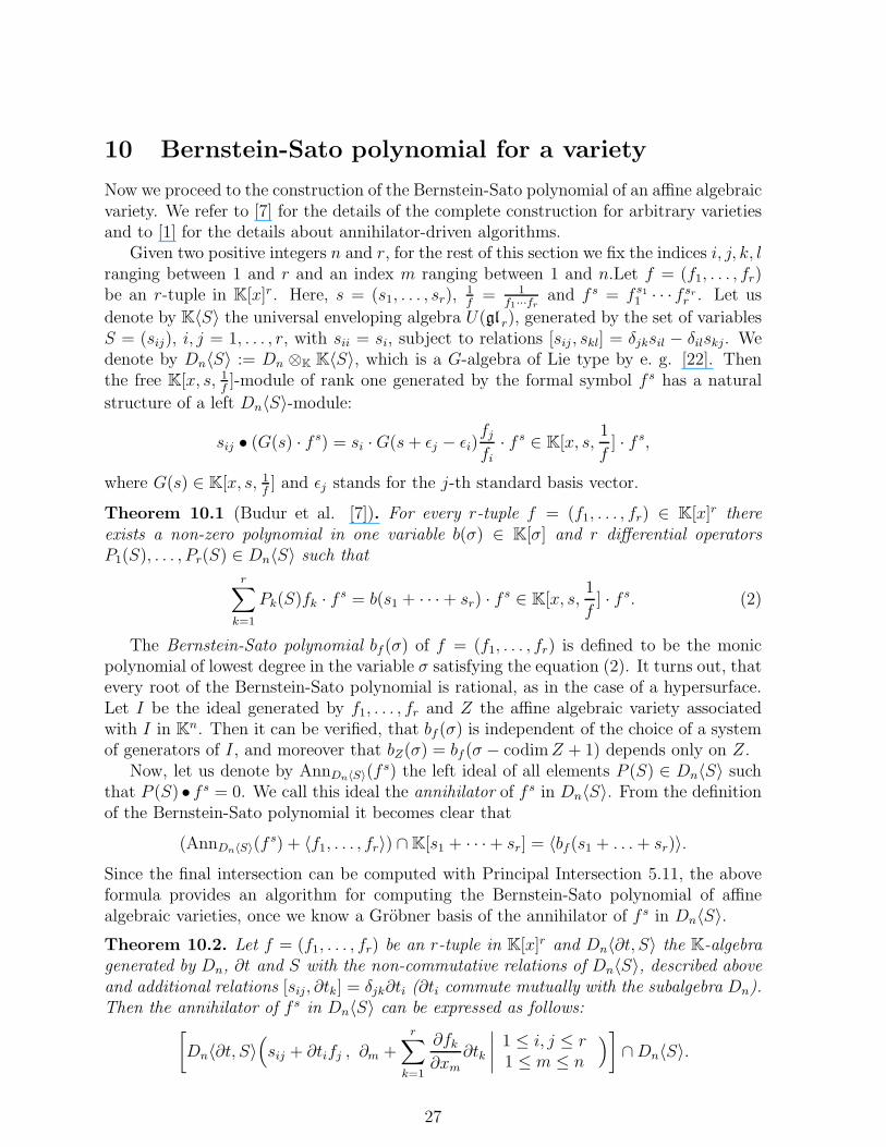
10 Bernstein-Sato polynomial for a variety

Now we proceed to the construction of the Bernstein-Sato polynomial of an affine algebraicvariety. We refer to [7] for the details of the complete construction for arbitrary varietiesand to [1] for the details about annihilator-driven algorithms.

Given two positive integers n and r, for the rest of this section we fix the indices i, j, k, lranging between 1 and r and an index m ranging between 1 and n.Let f = (f1, . . . , fr)be an r-tuple in K[x]r . Here, s = (s1, . . . , sr),

1f= 1

f1···frand f s = f s1

1 · · · f srr . Let us

denote by K〈S〉 the universal enveloping algebra U(gl r), generated by the set of variablesS = (sij), i, j = 1, . . . , r, with sii = si, subject to relations [sij , skl] = δjksil − δilskj. Wedenote by Dn〈S〉 := Dn ⊗K K〈S〉, which is a G-algebra of Lie type by e. g. [22]. Thenthe free K[x, s, 1

f]-module of rank one generated by the formal symbol f s has a natural

structure of a left Dn〈S〉-module:

sij • (G(s) · fs) = si ·G(s+ ǫj − ǫi)

fjfi

· f s ∈ K[x, s,1

f] · f s,

where G(s) ∈ K[x, s, 1f] and ǫj stands for the j-th standard basis vector.

Theorem 10.1 (Budur et al. [7]). For every r-tuple f = (f1, . . . , fr) ∈ K[x]r thereexists a non-zero polynomial in one variable b(σ) ∈ K[σ] and r differential operatorsP1(S), . . . , Pr(S) ∈ Dn〈S〉 such that

r∑

k=1

Pk(S)fk · fs = b(s1 + · · ·+ sr) · f

s ∈ K[x, s,1

f] · f s. (2)

The Bernstein-Sato polynomial bf (σ) of f = (f1, . . . , fr) is defined to be the monicpolynomial of lowest degree in the variable σ satisfying the equation (2). It turns out, thatevery root of the Bernstein-Sato polynomial is rational, as in the case of a hypersurface.Let I be the ideal generated by f1, . . . , fr and Z the affine algebraic variety associatedwith I in Kn. Then it can be verified, that bf (σ) is independent of the choice of a systemof generators of I, and moreover that bZ(σ) = bf (σ − codimZ + 1) depends only on Z.

Now, let us denote by AnnDn〈S〉(fs) the left ideal of all elements P (S) ∈ Dn〈S〉 such

that P (S) • f s = 0. We call this ideal the annihilator of f s in Dn〈S〉. From the definitionof the Bernstein-Sato polynomial it becomes clear that

(AnnDn〈S〉(fs) + 〈f1, . . . , fr〉) ∩K[s1 + · · ·+ sr] = 〈bf (s1 + . . .+ sr)〉.

Since the final intersection can be computed with Principal Intersection 5.11, the aboveformula provides an algorithm for computing the Bernstein-Sato polynomial of affinealgebraic varieties, once we know a Grobner basis of the annihilator of f s in Dn〈S〉.

Theorem 10.2. Let f = (f1, . . . , fr) be an r-tuple in K[x]r and Dn〈∂t, S〉 the K-algebragenerated by Dn, ∂t and S with the non-commutative relations of Dn〈S〉, described aboveand additional relations [sij, ∂tk] = δjk∂ti (∂ti commute mutually with the subalgebra Dn).Then the annihilator of f s in Dn〈S〉 can be expressed as follows:

[Dn〈∂t, S〉

(sij + ∂tifj , ∂m +

r∑

k=1

∂fk∂xm

∂tk

∣∣∣∣1 ≤ i, j ≤ r1 ≤ m ≤ n

)]∩Dn〈S〉.

27

Note, that this result and its proof [1] can be presented as natural generalization ofthe algorithm for computing AnnDn[s](f

s) with the method of Briancon-Maisonobe (cf.Section 3).

As Budur et al. point out [7, p. 794], the Bernstein-Sato polynomial for varietiescoincides, up to shift of variables, with the b-function in [34, p. 194], if the weight vectoris chosen appropriately, see also [37]. Algorithms for computing the b-function have beenalready discussed in Section 5, so the procedure bfctIdeal can be immediately applied tothis situation. Hence, like for the case of a hypersurface, we have two essentially differentways to compute Bernstein-Sato polynomials for varieties. The comparison of these twomethods is the subject of further research.

In the new Singular library dmodvar.lib1, we present the implementations of thefollowing algorithms

SannfsVar, which computes AnnDn〈S〉(fs) according to the Theorem 10.2,

bfctVarIn, which computes bf (s1 + . . .+ sr) using initial ideal approach,

bfctVarAnn, which computes bf (s1 + . . .+ sr) using annihilator-driven approach.

Example 10.3. Let TX = V (x20 + y30, 2x0x1 + 3y20y1) ⊂ C4 the tangent bundle of X =V (x2+y3) ⊂ C2. Then the Bernstein-Sato polynomial of TX can be computed as follows:

LIB "dmodvar.lib";

ring R = 0,(x0,x1,y0,y1),Dp;

ideal F = x0^2+y0^3, 2*x0*x1+3*y0^2*y1;

bfctVarAnn(F); // annihilator-driven approach

// alternatiely, one can run

bfctVarIn(F); // approach via initial ideal

In both cases we obtain the polynomial

bTX(σ) = (σ + 1)2(σ + 1/3)2(σ + 2/3)2(σ + 1/2)(σ + 5/6)(σ + 7/6).

The annihilator ideal can be computed via executing, in addition to the first 3 lines ofthe above code, the following code:

def S = SannfsVar(F); // returns a ring

setring S; // in this ring, ideal LD is the annihilator

option(redSB); LD = groebner(LD); // reduced GB of LD

There are 15 generators in the Grobner basis of AnnF s:

3y20∂x1 − 2x0∂y1, 3y20∂x0 + 6y0y1∂x1 − 2x0∂y0 − 2x1∂y1, x0y0∂x1∂y0 − x0y0∂x0∂y1 +x1y0∂x1∂y1−2x0y1∂x1∂y1, 3y0y1∂x

21−x0∂x1∂y0+x0∂x0∂y1−x1∂x1∂y1, 3x0y0y1∂x0∂x1∂y1+

6x0y21∂x

21∂y1 − x20∂x1∂y

20 + x20∂x0∂y0∂y1 − 2x0x1∂x1∂y0∂y1 + x0x1∂x0∂y

21 − x21∂x1∂y

21 +

3x1y0∂x21+3x0y1∂x

21−3y0y1∂x1∂y1, 6x0y

21∂x

21∂y0∂y1+3x0y0y1∂x

20∂y

21−3x1y0y1∂x0∂x1∂y

21+

6x0y21∂x0∂x1∂y

21−x

20∂x1∂y

30+x

20∂x0∂y

20∂y1−2x0x1∂x1∂y

20∂y1+x0x1∂x0∂y0∂y

21−x

21∂x1∂y0∂y

21+

3x1y0∂x21∂y0+3x0y1∂x

21∂y0+9x0y1∂x0∂x1∂y1−6y0y1∂x1∂y0∂y1+3y0y1∂x0∂y

21+6y21∂x1∂y

21+

1it will be distributed with the next release of Singular

28

3x1∂x21 + 3y1∂x1∂y1, 6x0y

21∂x

31∂y1 − x20∂x

21∂y

20 + 2x20∂x0∂x1∂y0∂y1 − 2x0x1∂x

21∂y0∂y1 −

x20∂x20∂y

21+2x0x1∂x0∂x1∂y

21−x

21∂x

21∂y

21−3x0y0∂x0∂x

21+3x1y0∂x

31+3x0y1∂x

31−2x0∂x1∂y0∂y1+

x0∂x0∂y21 −3x1∂x1∂y

21 +6y0∂x

21, s22−x1∂x1−y1∂y1, 6s21−3x0∂x1−2y0∂y1, 6s11−

3x0∂x0+3x1∂x1−2y0∂y0+4y1∂y1, s12x0+3y0y21∂x1−x0x1∂x0+x

21∂x1−x0y1∂y0, s12y0∂y1−

x1y0∂x1∂y0+2x1y1∂x1∂y1−y0y1∂y0∂y1+2y21∂y21−y0∂y0+4y1∂y1, 3s12y

20+6x1y0y1∂x1−

3y20y1∂y0+6y0y21∂y1−2x0x1∂y0, s12x1∂y

21−3s12y0∂x1+3x1y0y1∂x0∂x1∂y1+6x1y

21∂x

21∂y1−

3y0y21∂x1∂y0∂y1+3y0y

21∂x0∂y

21+6y31∂x1∂y

21−x0x1∂x1∂y

20+x0x1∂x0∂y0∂y1−2x21∂x1∂y0∂y1−

x1y1∂y0∂y21+3x1y0∂x0∂x1+3x1y1∂x

21−6y0y1∂x1∂y0+9y0y1∂x0∂y1+18y21∂x1∂y1−2x1∂y0∂y1+

3y0∂x0, 3s12y0y1∂x1−s12x1∂y1−3x1y0y1∂x0∂x1−3y0y21∂x0∂y1+x

21∂x1∂y0+x1y1∂y0∂y1−

3y0y1∂x0 + x1∂y0.

This ideal belongs to the K-algebra D4〈S〉 in 12 variables, as defined in the beginning ofthis section. By executing

GKdim(LD);

we obtain, that the Gel’fand-Kirillov dimension of D4〈S〉/AnnFs is 6, the half of the

Gel’fand-Kirillov dimension of D4〈S〉. However, D4〈S〉/AnnFs is not a generalized holo-

nomic D4〈S〉-module, since the annihilator of this module contains a central elements12s21 − s11s22 − s11 and hence is not zero.

References

[1] D. Andres, V. Levandovskyy, and J. Martın-Morales. Principal intersection andBernstein-Sato polynomial of an affine variety. In J. P. May, editor, Proc. of theInternational Symposium on Symbolic and Algebraic Computation (ISSAC’09), pages231–238. ACM Press, 2009.

[2] D. Andres, V. Levandovskyy, and J. Martın-Morales. Effective methods for thecomputation of Bernstein-Sato polynomials for hypersurfaces and affine varieties.http://arxiv.org/abs/1002.3644, 2010.

[3] R. Bahloul and T. Oaku. Local Bernstein-Sato ideals: algorithm and examples. J.Symbolic Computation, 45(1):46–59, 2010.

[4] I. N. Bernstein. Modules over a ring of differential operators. An investigation ofthe fundamental solutions of equations with constant coefficients. Functional Anal.Appl., 5(2):89–101, 1971.

[5] J. Briancon and P. Maisonobe. Remarques sur l’ideal de Bernstein associe a despolynomes. Preprint no. 650, Univ. Nice Sophia-Antipolis, 2002.

[6] M. Brickenstein. Slimgb: Grobner Bases with Slim Polynomials. In Rhine Workshopon Computer Algebra, pages 55–66, 2006. Proceedings of RWCA’06, Basel, March2006.

[7] N. Budur, M. Mustata, and M. Saito. Bernstein-Sato polynomials of arbitrary vari-eties. Compos. Math., 142(3):779–797, 2006.

29

[8] J. Bueso, J. Gomez-Torrecillas, and A. Verschoren. Algorithmic methods in non-commutative algebra. Applications to quantum groups. Kluwer Academic Publishers,2003.

[9] F. Castro-Jimenez and L. Narvaez-Macarro. Homogenising differential operators.Prepublicacion no. 36, Universidad de Sevilla, 1997.

[10] S. Coutinho. A primer of algebraic D-modules. Cambridge Univ. Press., 1995.

[11] W. Decker, G.-M. Greuel, G. Pfister, and H. Schonemann. Singular 3-1-1. A Com-puter Algebra System for Polynomial Computations. Centre for Computer Algebra,University of Kaiserslautern. http://www.singular.uni-kl.de, 2010.

[12] J. C. Faugere, P. Gianni, D. Lazard, and T. Mora. Efficient computation ofzero-dimensional Grobner bases by change of ordering. J. Symbolic Computation,16(4):329–344, 1993.

[13] J. Gago-Vargas, M. Hartillo-Hermoso, and J. Ucha-Enrıquez. Comparison of theo-retical complexities of two methods for computing annihilating ideals of polynomials.J. Symbolic Computation, 40(3):1076–1086, 2005.

[14] G.-M. Greuel, V. Levandovskyy, and H. Schonemann. Plural. A Singular 3-1-0Subsystem for Computations with Non-commutative Polynomial Algebras. Centre forComputer Algebra, University of Kaiserslautern. http://www.singular.uni-kl.de,2006.

[15] G.-M. Greuel and G. Pfister. A SINGULAR Introduction to Commutative Algebra.Springer, 2nd edition, 2008. With contributions by O. Bachmann, C. Lossen andH. Schonemann.

[16] M. I. Hartillo-Hermoso. About an algorithm of T. Oaku. In Ring theory and algebraicgeometry (Leon, 1999), volume 221 of Lecture Notes in Pure and Appl. Math., pages241–250. Dekker, New York, 2001.

[17] A. Kandri-Rody and V. Weispfenning. Non-commutative Grobner bases in algebrasof solvable type. J. Symbolic Computation, 9(1):1–26, 1990.

[18] M. Kashiwara. B-functions and holonomic systems. Rationality of roots of B-functions. Invent. Math., 38(1):33–53, 1976/77.

[19] V. Levandovskyy. On preimages of ideals in certain non–commutative algebras. InG. Pfister, S. Cojocaru, and V. Ufnarovski, editors, Computational Commutative andNon-Commutative Algebraic Geometry. IOS Press, 2005.

[20] V. Levandovskyy and J. Martın-Morales. Computational D-module theory withsingular, comparison with other systems and two new algorithms. In Proc. of theInternational Symposium on Symbolic and Algebraic Computation (ISSAC’08). ACMPress, 2008.

30

[21] V. Levandovskyy and J. Martın-Morales. Algorithms for checking rational roots ofb-functions and their applications. http://arxiv.org/abs/1003.3478, 2010.

[22] V. Levandovskyy and H. Schonemann. Plural — a computer algebra system fornoncommutative polynomial algebras. In Proc. of the International Symposium onSymbolic and Algebraic Computation (ISSAC’03), pages 176 – 183. ACM Press, 2003.

[23] H. Li. Noncommutative Grobner bases and filtered-graded transfer. Springer, 2002.

[24] B. Malgrange. Le polynome de Bernstein d’une singularite isolee. In Fourier inte-gral operators and partial differential equations (Colloq. Internat., Univ. Nice, Nice,1974), pages 98–119. Lecture Notes in Math., Vol. 459. Springer, Berlin, 1975.

[25] Z. Mebkhout. Sur le theoreme de finitude de la cohomologie p-adique d’une varieteaffine non singuliere. Amer. J. Math., 119(5):1027–1081, 1997.

[26] Z. Mebkhout and L. Narvaez-Macarro. Le theoreme de continuite de la division dansles anneaux d’operateurs differentiels. J. Reine Angew. Math., 503:193–236, 1998.

[27] H. Nakayama. Algorithm computing the local b function by an approximate division

algorithm in D. J. Symbolic Computation, 44(5):449–462, 2009. Spanish NationalConference on Computer Algebra.

[28] L. Narvaez-Macarro. Linearity conditions on the Jacobian ideal and logarithmic-meromorphic comparison for free divisors. In Singularities I, Algebraic and AnalyticAspects, pages 245–269. Contemporary Mathematics, 474, AMS, 2008.

[29] K. Nishiyama and M. Noro. Stratification associated with local b-functions. J.Symbolic Computation, 45(4):462 – 480, 2010.

[30] M. Noro. An efficient modular algorithm for computing the global b-function. InMathematical software (Beijing, 2002), pages 147–157. World Sci. Publ., River Edge,NJ, 2002.

[31] M. Noro, T. Shimoyama, and T. Takeshima. Risa/Asir, an open source generalcomputer algebra system. http://www.math.kobe-u.ac.jp/Asir, 2006.

[32] T. Oaku. Algorithms for the b-function and D-modules associated with a polynomial.J. Pure Appl. Algebra, 117/118:495–518, 1997.

[33] M. Saito. On microlocal b-function. Bull. Soc. Math. France, 122(2):163–184, 1994.

[34] M. Saito, B. Sturmfels, and N. Takayama. Grobner deformations of hypergeomet-ric differential equations, volume 6 of Algorithms and Computation in Mathematics.Springer-Verlag, Berlin, 2000.

[35] K. Schindelar, V. Levandovskyy, and E. Zerz. Exact linear modeling using Orealgebras. J. Symbolic Computation, 2010. To appear.

31

[36] M. Schulze. A normal form algorithm for the Brieskorn lattice. J. Symbolic Compu-tation, 38(4):1207–1225, 2004.

[37] T. Shibuta. An algorithm for computing multiplier ideals. http://arxiv.org/abs/math/0807.4302, 2008.

[38] N. Takayama. kan/sm1, a Grobner engine for the ring of differential and differenceoperators. http://www.math.kobe-u.ac.jp/KAN/index.html, 2003.

[39] T. Torrelli. Logarithmic comparison theorem and D-modules: an overview. In Sin-gularity theory, pages 995–1009. World Sci. Publ., Hackensack, NJ, 2007.

[40] H. Tsai and A. Leykin. D-modules package for Macaulay 2 – algorithms for D–modules. http://www.ima.umn.edu/~leykin/Dmodules, 2006.

[41] A. N. Varchenko. Asymptotic Hodge structure on vanishing cohomology. Izv. Akad.Nauk SSSR Ser. Mat., 45(3):540–591, 1981.

Acknowledgements

We would like to thank Francisco Castro-Jimenez, Jose-Marıa Ucha, Gert-Martin Greuel,Enrique Artal, Jose-Ignacio Cogolludo and Luis Narvaez for fruitful discussions and in-sightful remarks concerning our work.

Daniel AndresLehrstuhl D fr Mathematik, RWTH Aachen, Templergraben 64, 52062 Aachen, Germanye-mail: Daniel.Andres@math.rwth-aachen.de

Michael BrickensteinMathematisches Forschungsinstitut Oberwolfach, Schwarzwaldstr. 9-11, 77709 Oberwolfach-Walke, Germanye-mail: brickenstein@mfo.de

Viktor LevandovskyyLehrstuhl D fr Mathematik, RWTH Aachen, Templergraben 64, 52062 Aachen, Germanye-mail: Viktor.Levandovskyy@math.rwth-aachen.de

Jorge Martn-MoralesDepartment of Mathematics-I.U.M.A., University of Zaragoza, C/ Pedro Cerbuna, 12 -50009, Zaragoza, Spaine-mail: jorge@unizar.es

Hans SchnemannFachbereich Mathematik, TU Kaiserslautern, Erwin-Schrdinger-Str. 48, 67632 Kaiser-slautern, Germanye-mail: hannes@mathematik.uni-kl.de

32