a “discretization” technique for the solution of odes ii

PLEASE SCROLL DOWN FOR ARTICLE

This article was downloaded by: [HEAL-Link Consortium]On: 12 July 2009Access details: Access Details: [subscription number 772810551]Publisher Taylor & FrancisInforma Ltd Registered in England and Wales Registered Number: 1072954 Registered office: Mortimer House,37-41 Mortimer Street, London W1T 3JH, UK

Numerical Functional Analysis and OptimizationPublication details, including instructions for authors and subscription information:http://www.informaworld.com/smpp/title~content=t713597287

A “Discretization” Technique for the Solution of ODEs IIEugenia N. Petropoulou a; Panayiotis D. Siafarikas b; Efstratios E. Tzirtzilakis c

a Department of Engineering Sciences, Division of Applied Mathematics and Mechanics, University of Patras,Patras, Greece b Department of Mathematics, University of Patras, Patras, Greece c Department ofMechanical Engineering and Water Resources, Technological Educational Institute of Messolonghi,Messolonghi, Greece

Online Publication Date: 01 May 2009

To cite this Article Petropoulou, Eugenia N., Siafarikas, Panayiotis D. and Tzirtzilakis, Efstratios E.(2009)'A “Discretization” Techniquefor the Solution of ODEs II',Numerical Functional Analysis and Optimization,30:5,613 — 631

To link to this Article: DOI: 10.1080/01630560902987576

URL: http://dx.doi.org/10.1080/01630560902987576

Full terms and conditions of use: http://www.informaworld.com/terms-and-conditions-of-access.pdf

This article may be used for research, teaching and private study purposes. Any substantial orsystematic reproduction, re-distribution, re-selling, loan or sub-licensing, systematic supply ordistribution in any form to anyone is expressly forbidden.

The publisher does not give any warranty express or implied or make any representation that the contentswill be complete or accurate or up to date. The accuracy of any instructions, formulae and drug dosesshould be independently verified with primary sources. The publisher shall not be liable for any loss,actions, claims, proceedings, demand or costs or damages whatsoever or howsoever caused arising directlyor indirectly in connection with or arising out of the use of this material.

http://www.informaworld.com/smpp/title~content=t713597287

http://dx.doi.org/10.1080/01630560902987576

http://www.informaworld.com/terms-and-conditions-of-access.pdf

Numerical Functional Analysis and Optimization, 30(5–6):613–631, 2009Copyright © Taylor & Francis Group, LLCISSN: 0163-0563 print/1532-2467 onlineDOI: 10.1080/01630560902987576

A “DISCRETIZATION” TECHNIQUE FOR THE SOLUTION OF ODEs II

Eugenia N. Petropoulou,1 Panayiotis D. Siafarikas,2

and Efstratios E. Tzirtzilakis3

1Department of Engineering Sciences, Division of Applied Mathematics and Mechanics,University of Patras, Patras, Greece2Department of Mathematics, University of Patras, Patras, Greece3Department of Mechanical Engineering and Water Resources,Technological Educational Institute of Messolonghi, Messolonghi, Greece

� A functional analytic technique was recently presented for finding discrete equivalentcounterparts of initial value problems of ODEs and obtaining their real analytic solutions. Inthe current paper, this technique is extended to boundary value problems of ODEs and to thecomplex solutions of ODEs. In order to demonstrate this technique, it is applied to the classicBlasius problem of fluid mechanics. Apart from its real solution, its complex solution is alsostudied. The obtained results indicate that the complex Blasius function exhibits an oscillatorybehavior and strengthen a conjecture regarding its singularities in the complex plane.

Keywords Analytic structure; Blasius; Complex solution; Functional-analytic method;Singularities.

Mathematics Subject Classification 34A12; 34A25; 34B15; 34M10; 34M99; 65L10;76M25; 76M40.

1. INTRODUCTION

In [1], a functional-analytic technique was introduced for thediscretization of initial value problems of (system of) nonlinear ordinarydifferential equations. This technique is based on the equivalenttransformation of (system of) ordinary differential equation(s), toa (system of) difference equation(s), through an operator equation(or system of operator equations), via specific isomorphisms. As anapplication, the real analytic solutions of the Duffing oscillator equation

Address correspondence to Eugenia N. Petropoulou, Department of Engineering Sciences,Division of Applied Mathematics and Mechanics, University of Patras, Patras 26500, Greece; E-mail:[email protected]

613

Downloaded By: [HEAL-Link Consortium] At: 08:44 12 July 2009

614 E. N. Petropoulou et al.

and the Lorenz system were evaluated. The obtained solutions were of theform

f (z) =∞∑n=1

fnzn−1, z ∈ [−T ,T ], T > 0� (1.1)

and the results were compared with numerical ones obtained using theclassic fourth order Runge–Kutta method, indicating that the method in[1] is better than the Runge–Kutta method, with respect to the accuracyand the CPU time required. Moreover, the advantages of this method arethat

(i) a discrete equivalent and not a discrete analogue of the (system of)differential equation(s) is obtained, which makes the method veryaccurate as the only errors involved are the round-off errors;

(ii) it is independent of the grid used; and(iii) it is very quick.

The study of the complex solutions of differential equations is quiteimportant because it can provide a further insight to their properties.For the general theory of ordinary differential equations in the complexdomain, one can consult the books [2, 3]. Complementary to thetheoretical study of complex differential equations, approximate methodsof solving them are also very useful. Indicatively, the papers [4–6] arementioned. Also, the analysis of the singularities of the solution of anordinary differential equation seems to be connected with the notion ofintegrability, and there are several studies of the complex time behavior ofthe solutions of certain dynamic systems (see, for example, the book [7,Chapter 8] and the papers [8–12]).

Moreover, complex analysis has also been used for the study of thesolutions of differential equations describing physical problems, suchas problems in fluid mechanics. It is noted that the most famousdimensionless parameter in a fluid mechanics problem is the Reynoldsnumber (R), which expresses the ratio of the inertia to the viscous forcesin the flow domain. Thus, from a “conventional” fluid mechanics approachviewpoint, the whole physical problem as well as the dimensionlessparameters such as the R number are defined in the real plane, and thecomplex plane seems to be totaly irrelevant to the true physical problem.However, as far as what the physical meaning of a complex solutioncould be, it is worth mentioning that in [13, 14], the correspondingfluid mechanical problems are studied by assuming that specific physicalquantities are complex, such as the R and the spatial variables! It ismentioned indicatively that the singularities in the complex R -plane arefound for the physical problem of the Oseen flow past a sphere in [13] and


“Discretization” Technique for Solution of ODEs II 615

the singularities in the spatial complex place as well as contours of the real,and imaginary part of the vorticity, for the 2D Euler flow at short times,are given in [14]. In [15], it is mentioned that “singularity formation canbe viewed as the motion of singularities in the complex physical space thatreach the real axis in finite time.” Thus, it seems that studying the physicalproblem in the complex plane could provide useful information about thereal physical problem itself. Furthermore, quoting [14] it is hoped that“there is something universal in the nature of the singularities, be it onlytheir very existence.”

The principal aim of the current paper is to extend the method of [1],to

(i) the study of boundary value problems of ordinary differentialequations; and

(ii) the evaluation of complex solutions of ordinary differential equations.

The first is accomplished by combining the technique in [1] witha classic “shooting” method and solving, instead of the boundary valueproblem under consideration, a “sequence” of associated initial valueproblems. The second is accomplished by making the simple observationthat the coefficients fn of (1.1) can be written in the form fn = un + ivn andthe independent variable z (which is now a complex variable in the disk|z| < T ) in the polar form z = re i�.

In order to demonstrate the proposed technique, this is applied tothe classic Blasius problem, which consists of the nonlinear ordinarydifferential equation:

f ′′′(�) + 12f (�)f ′′(�) = 0, � > 0, (1.2)

the initial conditions

f (0) = f ′(0) = 0 (1.3)

and the boundary condition

f ′(+∞) = 1� (1.4)

This is a fundamental problem in fluid mechanics and it is actually the firstexample illustrating the application of Prandtl’s boundary-layer theory.More precisely, it appears in the study of the two-dimensional laminarsteady boundary layer flow, in the absence of pressure variations, over asemi-infinite flat plate parallel to the x -axis, with a free stream velocity alsoparallel to the x -axis. The boundary value problem (1.2)–(1.4) is obtained



from the simplified Navier–Stokes equations known as Prandtl’s boundarylayer equations, after using a similarity transformation. The unknown fstands for the dimensionless stream function, whereas f ′ is connected withthe horizontal velocity of the fluid, and this indicates the need to study asmuch as possible the behavior of f ′. (For more details, see, for example,[16, mainly Chapters VII–X]).

Apart from Blasius himself [17] in 1908, many researchers have studiedthe solution of the Blasius problem (1.2)–(1.4) (which shall be calledfrom now on the Blasius function), with various analytic, approximate, ornumerical methods. Blasius found a power series solution of (1.2)–(1.4)around � = 0 as well as an asymptotic expansion of its solution for large� and matched them at a specific finite value of � in order to obtain anapproximation of the Blasius function. For the numerical investigation ofthe Blasius function, one problem that had to be solved was to derive agood approximation of the third initial condition f ′′(0), which would giverise to a solution of (1.2) satisfying the two given initial conditions (1.3)and the boundary condition (1.4). For a concise history of the Blasiusproblem, see [16, 18] as well as the references therein.

Although for the physical problem already discussed, the independentvariable � must be positive, there are a few studies on the Blasius functionfor � < 0 or � ∈ �. More precisely in [19], the solutions of (1.2)–(1.3) arediscussed for � < 0 and various boundary conditions. Also, the behaviorof the Blasius function in the complex plane was studied in [18]. Moreprecisely in [18], several numerical constants were calculated and anexpansion of the Blasius function in rational Chebyshev functions wasderived. Also it was found that the Blasius function has a singularity at

� = −5�6900380545

and near it there is an infinite series of logarithmic corrections. Theexistence of a pole (for the Blasius function), its residue, and itsapproximate location was already found in [20]. Moreover in [18], acartography of the complex plane for the Blasius function was studied andtwo conjectures were made regarding its singularities:

1st Conjecture: “All singularities of the Blasius function lie withinthe radial sector � ∈ [�/4, 5�/12] plus the two sectors obtained from thisby rotation about the origin in the complex plane through angles of 2�/3and 4�/3.”

2nd Conjecture: “There is an infinite number of singularities andthe locations of these asymptotes to the ray arg � = �/4 (and the fivecorresponding rays in other sectors) as |�| → ∞.”



The above studies of the Blasius problem for � ∈ � make thisproblem a good benchmark for a representative application of thecurrent “discretization” technique for the solution of ordinary differentialequations in the complex plane. Thus, by applying the proposed techniqueto the Blasius problem, it is proved that there exists a unique analyticsolution of (1.2)–(1.4), of the form f (�) = ∑∞

n=1 �n�n−1, which together

with its first two derivatives converge absolutely for every � ∈ � with|�| < T , T > 0. Moreover, both its real and complex valued solutions areevaluated. More precisely, in the case where � ∈ � (see Section 3), therequired third initial condition f ′′(0) = � is determined to be

� = 0�33205733621519678555,

which coincides with the first 15 decimal points of the value found in [18].Also it is found that the Blasius function has a singularity at ��−5�69,which, according to [18, 20], is a simple pole.

In the case where � ∈ � (see Section 4), the results indicate that theBlasius problem has a unique analytic solution outside the radial sectors� = [45◦, 75◦], [165◦, 195◦], and [285◦, 315◦] of the complex plane. Thismeans that if the Blasius function has singularities, those should lie insidethe radial sectors � = [45◦, 75◦], [165◦, 195◦], and [285◦, 315◦]. Indeed, thisis confirmed by the numerical results, which give the location of the firstsingularity of the Blasius function in various directions of the complexplane inside the above-mentioned sectors. These results strengthen thefirst conjecture of [18]. Unfortunately, the method used cannot give anyinformation regarding the kind or the total number of the singularities.

Furthermore, it is obvious that the Blasius function does not “blow-up” in those regions of the complex plane where it is analytic. It is worthmentioning here that the blowing-up solutions of the problem

f ′′′(�) + f (�)f ′′(�) = 0, � ∈ (0, �c)

f (0) = 1, f ′(0) = 0, f ′′(0) = c < 0,

which is similar to (1.2)–(1.4), were studied in [21] and the referencestherein.

2. THE METHOD

As already mentioned in the introduction, the technique that willbe used in the current paper for the study of the Blasius problem isbased on a functional analytic method introduced in [1]. More precisely,the main idea is to transform the ordinary differential equation underconsideration, i.e., the Blasius equation, into an equivalent operator



equation in an abstract Banach space and from this to deduce anequivalent difference equation, which is the “numerical scheme” usedin order to obtain an exact solution of the Blasius problem. Themethod can be applied only when the ordinary differential equationunder consideration is studied in the Banach space H1(�) of analyticfunctions defined in � = �z ∈ � : |z| < 1. Moreover, the solution of theequivalent difference equation, which gives eventually the solution ofthe corresponding differential equation, belongs to the Banach spaceof absolutely summable sequences, 1. The spaces H1(�) and 1 arecompletely defined in the next section.

It should also be mentioned that in [22], the analytic solutions inH1(�) of some nonlinear ordinary differential equations were studied.Among the studied equations there was the following general equation

f ′′′(�) + �(�)f (�)f ′′(�) + �(�)[1 − (f ′(�))2] = g (�), |�| < T , T ∈ (0,∞)(2.1)

which includes the Blasius equation (1.2). For (2.1) and (1.2), a theorem(Theorem 3.1 of [22]) and a corresponding corollary (Corollary 3.5of [22]) were proved establishing a unique solution of the formf (�) = ∑∞

n=1 �n�n−1, which together with its first two derivatives converge

absolutely for every � ∈ � with |�| < T . As mentioned in [22], theobtained results remain true for � ∈ �. (The exact results about the Blasiusproblem are quoted in Section 2.2.)

2.1. Basic Definitions and Propositions

First of all, define the Hilbert space H2(�) and the Banach spacesH1(�) and 1, where � = �z ∈ � : |z| < 1 by

H2(�) ={f : � → �/f (z) =

∞∑n=1

fnzn−1 analytic in � with∞∑n=1

|fn |2 < +∞}

H1(�) ={f : � → �/f (z) =

∞∑n=1

fnzn−1 analytic in � with∞∑n=1

|fn | < +∞}

and

1 ={fn : � → � with

∞∑n=1

|fn | < +∞}�

Denote now by H an abstract separable Hilbert space over the complexfield, with the orthonormal base �en, n = 1, 2, 3, � � � . Denote by 〈·, ·〉and ‖ · ‖ the inner product and the norm in H , respectively.



Define also in H the shift operator V :

Ven = en+1, n = 1, 2, 3, � � �

and its adjoint V ∗:

V ∗en = en−1, n = 2, 3, � � � , V ∗e1 = 0,

as well as the diagonal operator C0:

C0en = nen , n = 1, 2, 3, � � � �

The following enable the transition from the ordinary differentialequation to an equivalent operator equation (see [23, 24]):

Proposition 2.1. The representation

〈fz , f 〉 =∞∑n=1

fnzn−1 = f (z), z ∈ �, (2.2)

is a one-by-one mapping from H onto H2(�) that preserves the norm, wherefz = ∑∞

n=1 zn−1en, f0 = e1, is the complete system in H of eigenvectors of V ∗ and

f = ∑∞n=1 fnen an element of H .

The unique element f = ∑∞n=1 fnen appearing in (2.2) is called the

abstract form of f (z) in H . In general, if G(f (z)) is a function from H2(�)

to H2(�) and N (f ) is the unique element in H for which

G(f (z)) = 〈fz ,N (f )〉,

then N (f ) is called the abstract form of G(f (z)) in H .Consider now the linear manifold of all f (z) ∈ H2(�) that satisfy the

condition∑∞

n=1 |fn | < +∞. Define the norm

‖f (z)‖H1(�) =∞∑n=1

|fn |�

Then this manifold becomes the Banach space H1(�) defined before.Denote also by H1 the corresponding, by the representation (2.2), abstractBanach space of the elements f = ∑∞

n=1 fnen ∈ H for which∑∞

n=1 |fn | <+∞. (A detailed analysis, why we restrict to H1(�) and how H1(�) isconnected with H2(�), is given in [25, p. 385].)



The following properties hold [26, pp. 348–349].

(1) H1 is invariant under the operators V k , (V ∗)k , k = 1, 2, 3, � � � .(2) H1 is invariant under every bounded diagonal operator.

The abstract forms of the most common quantities appearing usually inordinary differential equations have been found in [22–26]. For the Blasiusproblem, only the following are needed:

(1) The abstract form of f ′′′(z) is the element (C0V ∗)3f , i.e.,

f ′′′(z) = 〈fz , (C0V ∗)3f 〉�(2) The abstract form of f (z)f ′′(z) is the element 1

2(C0V ∗)2f1(V )f −f ′1 (V )C0V ∗f , i.e.,

f (z)f ′′(z) =⟨fz ,

12(C0V ∗)2f1(V )f − f ′

1 (V )C0V ∗f⟩,

where f1(V ) = ∑∞n=1 fnV

n−1 and f ′1 (V ) = ∑∞

n=2(n − 1)fnV n−2.

Finally, the next proposition enables the transition from an operatorequation to an equivalent difference equation:

Proposition 2.2 ([27]). The linear function

� : H1 → 1

defined by

�(f ) = 〈f , en〉 = fn (2.3)

is an isomorphism from H1 onto 1, i.e., it is a 1–1 mapping from H1 onto 1,which preserves the norm.

2.2. Description of the Method

In the following, the method of [1] is described by applying it to theBlasius equation:

f ′′′(�) + 12f (�)f ′′(�) = 0, |�| < T , T > 0� (2.4)

Step 1. Reduce (2.4) to |z| < 1 by using the simple transformationz = �

T , f (�) = f (zT ) = F (z). Then (2.4) becomes

F ′′′(z) + T2F (z)F ′′(z) = 0, |z| < 1, (2.5)



and the initial conditions for F take the form:

F (0) = f (0), F ′(0) = Tf ′(0), F ′′(0) = T 2f ′′(0)�

(If T = 1, Step 1 is omitted.)

Step 2. Use the isomorphism (2.2) and rewrite (2.5) in the form ofan inner product in H1. Then (2.4) is rewritten as⟨

fz , (C0V ∗)3F + T4(C0V ∗)2F1(V )F − T

2F ′1(V )C0V ∗F

⟩= 0� (2.6)

Step 3. Use the completeness of �fz, |z| < 1 and find from (2.6) theequivalent to (2.4) operator equation in H1. For the Blasius equation, thisoperator equation is

(C0V ∗)3F + T4(C0V ∗)2F1(V )F − T

2F ′1(V )C0V ∗F = 0� (2.7)

Step 4. Take the inner product of both parts of (2.7) with en anduse (2.3) in order to obtain the equivalent to (2.7) difference equation.For the Blasius equation, its equivalent difference equation (“numericalscheme”) is

Fn = − T4(n − 1)

n−1∑k=1

FkFn−k + T2(n − 1)(n − 2)(n − 3)

×n−1∑k=2

(k − 1)(n − k − 1)FkFn−k , ∀n ≥ 4 (2.8)

F1 = F (0), F2 = F ′(0), F3 = 12F ′′(0)�

(Relation (2.8) was derived in [22].)

Step 5. Compute Fn from (2.8) and find

F (x) =∞∑n=1

Fnxn−1 ⇔ f (�) =∞∑n=1

Fn( �

T

)n−1� (2.9)

In this way, a “numerical scheme” is found for the Blasius equation.From this “numerical scheme,” the coefficients Fn are found and thus thetruncated solution

f (�) =N∑

n=1

Fn( �

T

)n−1, |�| < T ,

where N , a finite number, can be obtained.



2.2.1. Choice of N and TChoice of N . In order to determine N , the fact that the coefficients

Fn of (2.9) form a sequence belonging in 1 must be taken intoconsideration. Thus due to the definition of 1, the coefficients Fnsatisfy limn→∞ Fn = 0. Practically, this means that after some n = m, thecoefficients Fn computed by the method in Step 5 will be very small,practically zero (within the round-off error of the computer). Thus N canbe chosen greater or equal to m.

Choice of T . In order to choose T , equation (2.7) must bestudied in H1 and conditions should be obtained so that (2.7) has aunique solution in H1. In order to do this, the use of fixed pointtheorems and the manipulation of (2.7) are needed. The obtainedconditions are inequalities involving only T and the initial conditionsaccompanying (2.5). From these conditions, a suitable value for T canbe obtained. These conditions were found in [22] for the equation (2.1),which for the Blasius equation take the form:

T(3 + 5|F ′(0)| + 4|F (0)|) < 6 (2.10)

and

12|F ′′(0)| + T

6|F ′(0)|2 + T

4|F (0)| · |F ′(0)| + T

12|F (0)|2

<3

T(3 + 5|F ′(0)| + 4|F (0)|) (2.11)

More precisely, the result of [22] for the Blasius equation is: “if (2.10) and(2.11) hold, then the Blasius equation has a unique analytic solution of theform (2.9) which together with its first two derivatives converge absolutelyin the interval |�| < T .”

2.2.2. The Case Where � ∈ ��In this case, the truncated solution is given by

f (�) =N∑

n=1

Fn( �

T

)n−1, |�| < T

and T is chosen via the inequalities (2.10) and (2.11), where | · | stands forthe absolute value.

2.2.3. The Case Where � ∈ ��In this case, one should take into consideration the fact that the

coefficients Fn are in general complex, i.e., Fn = un + ivn . Also, because



� ∈ �, it can be represented in the polar form � = re i�. Thus the truncatedsolution is given now by

f (�) =N∑

n=1

r n−1

T n−1 un cos((n − 1)�) − vn sin((n − 1)�)�

+ iN∑

n=1

r n−1

T n−1 un sin((n − 1)�) + vn cos((n − 1)�)� ,

where |�| < T and T is chosen via the inequalities (2.10) and (2.11), wherenow | · | stands for the modulus. The coefficients un and vn are found from(2.8) by substituting Fn = un + ivn and equating the corresponding realand imaginary parts. More precisely, it is

un = − T4(n − 1)

(u1un−1 − v1vn−1)

+ Tn − 1

n−1∑k=2

[(k − 1)(n − k − 1)2(n − 2)(n − 3)

− 14

](ukun−k − vkvn−k), ∀n ≥ 4

(2.12)

u1 = Re F (0), u2 = Re F ′(0), u3 = 12Re F ′′(0)

and

vn = − T4(n − 1)

(u1vn−1 + v1un−1)

+ Tn − 1

n−1∑k=2

[(k − 1)(n − k − 1)2(n − 2)(n − 3)

− 14

](ukvn−k + vkun−k), ∀n ≥ 4

(2.13)

u1 = Im F (0), u2 = Im F ′(0), u3 = 12Im F ′′(0)�

3. THE BLASIUS FUNCTION IN THE REAL AXIS

First, the Blasius function in the real axis (� ∈ �) is considered.In order to solve the Blasius problem (1.2)–(1.4) with the methodintroduced in [1], a third initial condition f ′′(0) = � should bedetermined. This is necessary because the used method concerns thesolution of initial value problems. The procedure followed is the so-called“shooting” method, which is extensively used along with the Runge–Kuttamethod for the solution of such boundary value problems. The philosophyof this method is the following. First, take a random � and integratefor initial conditions f (0) = f ′(0) = 0, f ′′(0) = � up to an � = �max that



is chosen sufficiently large, most of the times depending on the physicalproblem. It is clearly assumed that for � > �max , the solution remains thesame and that f (�max) ≈ f (∞). Then, the value f (�max) is obtained and iscompared with the desired condition f ′(�max) = 1. Finally, � is adjusted insuch a way so as when the solution of the problem with initial values f (0) =f ′(0) = 0 and f ′′(0) = � is obtained, it will satisfy the relation f ′(�max) = 1.

In order to proceed to the numerical solution of the differentialequation (1.2) subject to the conditions f (0) = f ′(0) = 0 and f ′′(0) = �,the procedure followed in [1] is considered. The first step is to determineT from the relations (2.10) and (2.11). Then, the coefficients Fn aredetermined from (2.8) and the solution is obtained by the use of (2.9).One way to determine N for the numerical procedure is to monitor thecoefficients Fn during their calculation. It can be set, for example, that iffive successive coefficients are below 10−20, then N is sufficiently large. Itis recalled that the sequence of the coefficients decays to zero. Indicativevalues of N and T for the current problem are 43 and 1�87, respectively.Once the solution is calculated for the corresponding T , up to � = �1the quantities f (�1), f ′(�1), and f ′′(�1) are known. A new T is determinedas described above, and the solution is now calculated up to a point �2,with initial conditions the corresponding known values of f (�1), f ′(�1), andf ′′(�1). This procedure is followed until �max has been reached and thusthe value of f ′(�max) is obtained. The “shooting” method described aboveis used in order to adjust � so that the value f ′(�max) = 1.

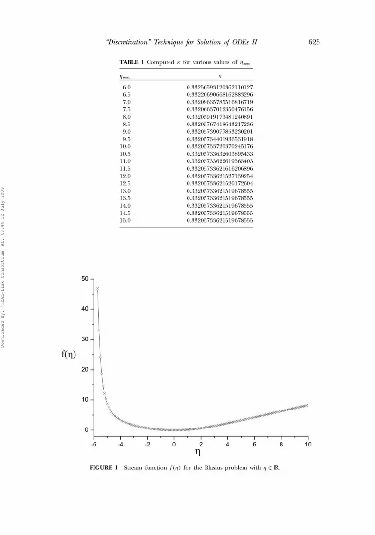
The above procedure is used in order to determine the value of � usingeach time for �max values ranging from 6 to 15. Table 1 shows the valuesof �max and the corresponding values of the obtained � so that f ′(�max)= 1.It is apparent that the calculated value of � changes as �max increases andthe final value is attained at �max = 13. For the Visual Fortran 6.6 usedon an AMD processor and Winxp platform, the number of digits thatprecede the exponent is unlimited, but typically only the left-most 15 digitsare significant. The obtained value of � = 0�33205733621519678555 agreeswith that calculated in [18] up to the 15th significant digit.

Figure 1 shows the calculated stream function f (�) for � ∈ �. It isapparent that the solution exhibits almost linear behavior for values of� � 5, decreases as � approaches to zero, where the minimum is attained,and increases for negative values of �. Also the function f (�) approaches∞ for � approaching −5�69. This indicates that the point � = −5�69 isa singularity of f (�). Indeed, it was verified in [18, 20] that the point� ≈ −5�69 is a simple pole for f (�). Moreover its residue was found in [20]to be 6. Figures 2 and 3 show the velocity f ′(�) for � ∈ �+ and for � ∈ �,respectively. From Figure 2, the well-known behavior of the velocity for theclassic Blasius problem (1.2)–(1.4) is observed, whereas from Figure 3 therapid decay of f ′(�) for � in the region of −5�69 can be observed.



TABLE 1 Computed � for various values of �max

�max �

6.0 0.332565931203621101276.5 0.332206906681628832967.0 0.332096357855168167197.5 0.332066370123504761568.0 0.332059191734812408918.5 0.332057674186432172369.0 0.332057390778532302019.5 0.33205734401936531918

10.0 0.3320573372037024517610.5 0.3320573363260389543311.0 0.3320573362261956540311.5 0.3320573362161620689612.0 0.3320573362152713925412.5 0.3320573362152017260413.0 0.3320573362151967855513.5 0.3320573362151967855514.0 0.3320573362151967855514.5 0.3320573362151967855515.0 0.33205733621519678555

FIGURE 1 Stream function f (�) for the Blasius problem with � ∈ �.



FIGURE 2 Velocity f ′(�) for the Blasius problem with � ∈ �+

FIGURE 3 Velocity f ′(�) for the Blasius problem with � ∈ �.



4. THE BLASIUS FUNCTION IN THE COMPLEX PLANE

The Blasius problem is now considered in the complex plane.The stream function f varies with the variable � = re i�. In an effort tolocate possible singularities in the complex plane, the Blasius functionis solved using the initial conditions Re f (0) = Re f ′(0) = 0, Re f ′′(0) = �and Im f (0) = Im f ′(0) = 0, Im f ′′(0) = 0, for various values of the angle� all over the complex plane ([0, 360◦]) and for r = 12. The variationstep of the angle � is 1◦. Figure 4 shows the location of singularitiesin the complex plane pictured in polar coordinates. It is apparent thatthe singularities lie within the sectors of � = [45◦, 75◦], [165◦, 195◦], and[285◦, 315◦]. This result has also been found in [18]. It is noted that onlythe first singularity can be detected in each sector and there is no ability,by using the current method, to examine the regions for larger r than thatfor which the first singularity is detected. For � = 180◦, the first singularity(in r = 5�69), detected in the real plane, is also evident. The center ofthe graph begins from r = 4 and the other closest singularities again forr = 5�69 are detected for � = 60◦ and 300◦. The same qualitatively resultsare obtained for r = 500 and angle step � = 0�05◦.

Figure 5 shows the variation of the Imaginary part (Im f ) with theReal part of the Blasius function (Re f ). The results are derived for anglestep of 10◦. The areas determined by the singularities, pictured in thefigure, are denoted with light gray. It is observed that for all �, sufficiently

FIGURE 4 Location of singularities in the complex plane (polar coordinates).



FIGURE 5 Variation of the imaginary part with the real part of the Blasius function.

far away from the regions where the singularities are located, Im f varieslinearly with Re f . As � increases, Im f starts to oscillate. This oscillationis obvious from values of � = 30◦ and increases when � approaches thevalue of 45◦ where the first singularities begin to appear. The two solutionspictured closest to the first area of the appearance of the singularities arefor � = 40◦ and 80◦, respectively. For the angles lying between the values� = 45◦ and 75◦, the solution follows a spiral motion.

Motivated by the fact that when discussing the solution of the Blasiusproblem in the real positive axis, f ′ plays an important role, as by a physicalpoint of view it expresses the velocity in the boundary layer, f ′ is alsoexamined in the complex plane. In that case, f ′ = Re f ′ + i Im f ′ and thevariation of the Imaginary part with the Real part of the derivative ofthe Blasius function is shown in Figure 6. The regions designated by theappearing singularities are also pictured with a light-gray pattern. The stepof the angle � of the presented results is again 10◦. The spiral motionsin the plane Re f ′ − Im f ′ are created for � = 50◦, 60◦, 170◦, 190◦, 290◦,and 310◦ as the Re f ′ and Im f ′ “diverge” to infinity. For all the othervalues of �, it is apparent that there are three points where the derivativeof the solution “converges.” This is more obvious in the magnificationprovided in Figure 7. The three points of convergence are (1, 0) and(−0�5,±0�866035).



FIGURE 6 Variation of the imaginary part with the real part of the derivative of the Blasiusfunction.

FIGURE 7 Variation of the imaginary part with the real part of the derivative of the Blasiusfunction.



It is observed that the behavior of the derivative of the Blasius functionis exactly the same in the region of the three aforementioned points.For this reason, the measure of the derivative (|f ′|) with the distancer (� = re i�) is presented graphically in Figure 8 for � = 20◦, 30◦, 40◦,and 50◦. For � = 0, the graph of the measure of the derivative is the oneof the real axis pictured in Figure 2. As � increases, |f ′| begins to oscillatebut finally reaches its asymptotic value of 1. The oscillations increase as� increases and finally for � = 50◦, which lies in the sector where thesingularities appear, |f ′| tends to infinity with the increment of r . It is alsoobserved that |f ′| tends to infinity through very specific “paths,” it does notpresent blow-ups, and the symmetry of the graphs is remained. It is worthmentioning here that the same behavior of |f ′| is observed for � = 340◦,330◦, 320◦, and 310◦, respectively. The interesting result is that the measureof the derivative behaves in an exactly analogous way in the region of theother two points that “attract” the derivative. This means that the graphof the measure of the derivative for � = 120◦ and 240◦ (pure complexplane) is the same with the graph of the derivative that is obtained in thereal axis for � = 0 (Fig. 2). Moreover, the behavior of |f ′|, as far as theoscillations are concerned, is analogous to that exhibited around � = 120◦

and � = 240◦, i.e., the same graphs are obtained for � = ±20◦, 120◦ ± 20◦,and 240◦ ± 20◦ as also demonstrated in Figure 8.

FIGURE 8 Variation of the measure of the derivative of the Blasius function (|f ′|) with the polardistance r for various angles.



REFERENCES

1. E.N. Petropoulou, P.D. Siafarikas, and E.E. Tzirtzilakis (2007). A “discretization” technique forthe solution of ODEs. J. Math. Anal. Appl. 331:279–296.

2. E. Hille (1997). Ordinary Differential Equations in the Complex Domain. Dover Publications,New York.

3. I. Laine (1992). Nevanlinna Theory and Complex Differential Equations. Walter de Gruyter & Co.,Berlin.

4. M. Gülsu and M. Sezer (2007). Approximate solution to linear complex differential equationby a new approximate approach. Appl. Math. Comput. 185:636–645.

5. M. Sezer and M. Gülsu (2006). Approximate solution of complex differential equations for arectangular domain with Taylor collocation method. Appl. Math. Comput. 177:844–851.

6. M. Sezer, M. Gülsu, and B. Tanay (2006). A Taylor collocation method for the numericalsolution of complex differential equations with mixed conditions in elliptic domains.Appl. Math. Comput. 182:498–508.

7. M. Tabor (1989). Chaos and Integrability in Nonlinear Dynamics. An Introduction. John Wiley &Sons, Inc., New York.

8. Y.F. Chang, J.M. Greene, M. Tabor, and J. Weiss (1983). The analytic structure of dynamicalsystems and self-similar natural boundaries. Phys. D. 8:183–207.

9. Y.F. Chang, M. Tabor, and J. Weiss (1982). On the analytic structure of the Henon-HeilesHamiltonian in integrable and nonintegrable regimes. J. Math. Phys. 23:531–538.

10. Y.F. Chang, M. Tabor, J. Weiss, and G. Corliss (1981). On the analytic structure of the Henon–Heiles system. Phys. Lett. A. 85:211–213.

11. A. Goriely and M. Tabor (1998). The role of complex-time singularities in chaotic dynamics.Regul. Chaotic Dyn. 3:32–44.

12. G. Levine and M. Tabor (1988). Integrating the nonintegrable: analytic structure of the Lorenzsystem revisited. Phys. D. 33:189–210.

13. C. Hunter and S.M. Lee (1986). The analytic structure of Oseen flow past a sphere as afunction of Reynolds number. SIAM J. Appl. Math. 46:978–999.

14. T. Matsumoto, J. Bec, and U. Frisch (2005). The analytic structure of 2D Euler flow at shorttimes. Fluid Dynam. Res. 36:221–237.

15. G.R. Baker, X. Li, and A.C. Morlet (1996). Analytic strucure of two 1D-transport equations withnonlocal fluxes. Phys. D. 91:349–375.

16. H. Schlichting (1987). Boundary-Layer Theory. McGraw-Hill, Inc., New York.17. H. Blasius (1908). Grenzschichten in flüssigkeiten mit kleiner reibung. Zeitschrift für Mathematik

und Physik 56:1–37.18. J.P. Boyd (1999). The Blasius function in the complex plane. Exp. Math. 8:381–394.19. J. Steinheuer (1968). Die lösungen der Blasiusschen grenzschichtdifferentialgleichung.

Proc. Wiss. Ges. Braunschweig. 20:96–125.20. B. Punnis (1956). Zur differentialgleichung der plattengrenzschicht von Blasius. Arch. Math.

7:165–171.21. N. Ishimura and S. Matsui (2003). On blowing-up solutions of the Blasius equation. Discrete

Contin. Dynam. Systems 9:985–992.22. E.N. Petropoulou and P.D. Siafarikas (2004). Analytic solutions of some non-linear ordinary

differential equations. Dynam. Systems Appl. 13:283–316.23. E.K. Ifantis (1970). Structure of the point spectrum of Schrödinger type tridiagonal operators.

J. Math. Phys. 11:3138–3144.24. E.K. Ifantis (1978). An existence theory for functional-differential equations and functional-

differential systems. J. Differential Equations 29:86–104.25. E.K. Ifantis (1987). Global analytic solutions of the radial nonlinear wave equation. J. Math.

Anal. Appl. 124:381–410.26. E.K. Ifantis (1987). Analytic solutions for nonlinear differential equations. J. Math. Anal. Appl.

124:339–380.27. E.K. Ifantis (1987). On the convergence of power series whose coefficients satisfy a Poincaré

type linear and nonlinear difference equation. Complex Variables 9:63–80.


a “discretization” technique for the solution of odes ii

Documents