2

Reinforcement Learning in System Identification Mariela Cerrada and Jose Aguilar

Universidad de los Andes Mérida-VENEZUELA

1. Introduction The Reinforcement Learning (RL) problem has been widely researched an applied in several areas (Sutton & Barto, 1998; Sutton, 1988; Singh & Sutton, 1996; Schapire & Warmuth, 1996; Tesauro, 1995; Si & Wang, 2001; Van Buijtenen et al., 1998). In dynamical environments, a learning agent gets rewards or penalties, according to its performance for learning good actions. In identification problems, information from the environment is needed in order to propose an approximate system model, thus, RL can be used for taking the on-line information taking. Off-line learning algorithms have reported suitable results in system identification (Ljung, 1997); however these results are bounded on the available data, their quality and quantity. In this way, the development of on-line learning algorithms for system identification is an important contribution. In this work, it is presented an on-line learning algorithm based on RL using the Temporal Difference (TD) method, for identification purposes. Here, the basic propositions of RL with TD are used and, as a consequence, the linear TD(λ) algorithm proposed in (Sutton & Barto, 1998) is modified and adapted for systems identification and the reinforcement signal is generically defined according to the temporal difference and the identification error. Thus, the main contribution of this paper is the proposition of a generic on-line identification algorithm based on RL. The proposed algorithm is applied in the parameters adjustment of a Dynamical Adaptive Fuzzy Model (DAFM) (Cerrada et al., 2002; Cerrada et al., 2005). In this case, the prediction function is a non-linear function of the fuzzy model parameters and a non-linear TD(λ) algorithm is obtained for the on-line adjustment of the DAFM parameters. In the next section the basic aspects about the RL problem and the DAFM are revised. Third section is devoted to the proposed on-line learning algorithm for identification purposes. The algorithm performance for time-varying non-linear systems identification is showed with an illustrative example in section fourth. Finally, conclusions are presented.

2. Theoretical background

2.1 Reinforcement learning and temporal differences RL deals with the problem of learning based on trial and error in order to achieve the overall objective (Sutton & Barto, 1998). RL are related to problems where the learning agent does not know what it must do. Thus, the agent must discover an action policy for maximize the

Reinforcement Learning: Theory and Applications

22

expected gain defined by the rewards that the agents gets. At time t, (t=0, 1, 2, ...), the agent receives the state St and based on this information it choises an action at. As a consequence, the agent receives a reinforcement signal or reward rt+1. In case of the infinite time domain, a discount weights the received reward and the discounted expected gain is defined as:

(1)

where μ, 0 < μ ≤ 1, is the discount rate, and it determines the current value of the futures rewards. On the other hand, TD method permits to solve the prediction problem taking into account the difference (error) between two prediction values at successive instants t and t+1, given by a function P. According to the TD method, the adjustment law for the parameter vector θ of the prediction function P(θ) in given by the following equation (Sutton, 1988) :

(2)

where xt is a vector of available data at time t and η, 0 < η ≤ 1, is the learning rate. The term between parentheses is the temporal difference and the equation (2) is the TD algorithm that can be used on-line in a incremental way. RL problem can be viewed as a prediction problem where the objective is the estimation of the discounted gain defined by equation (1), by using the TD algorithm. Let be the prediction of Rt . Then, from equation (1):

(3)

The real value of Rt+1 is not available, then, by replacing it by its estimated value in (3), the prediction error is defined by the following equation:

(4)

which describe a temporal difference. The reinforcement value rt+1 is defined in order to obtain at time t+1 a better prediction of Rt , given by , based on available information. In this manner, a good estimation in the RL problem means the optimization of Rt . Thus, denoting as P and by replacing the temporal difference in (2) by that one defined in (4), the parameters adjustment law is:

(5)

The learning agent using the equation (5) for the parameters adjustment is called Adaptive-Heuristic-Critic (Sutton & Barto, 1998). In on-line applications, the time t is the same iteration time in the learning process by using equation (5).

tR̂

R̂

tR̂

Reinforcement Learning in System Identification

23

2.2 Dynamical adaptive fuzzy models Without loss of generality, a fuzzy logic model MISO (Multiple Inputs-Single Output), is a linguistic model defined by the following M fuzzy rules:

(6) where xi is a vector of linguistic input on the domain of discourse Ui ; y is the linguistic output variable on the domain of discourse V; Fil and Gl are fuzzy sets on Ui and V, respectively, (i=1,... ,n) and (l=1,... ,M), each one defined by their membership functions. The DAFM is obtained from the previous rule base (6), by supposing input values defined by fuzzy singleton, gaussian membership functions of the fuzzy sets defined for the fuzzy output variables and the defuzzification method given by center-average method. Then, the inference mechanism provides the following model (Cerrada et al., 2005):

(7)

where X=(x1 x2 ... xn)T is a vector of linguistic input variables xi at time t; α( vil,tj), β( wil,tj) and γ( ul,tj) are time-depending functions; vil and wil are parameters associated to the variable xi in the rule l; ul is a parameter associated to the center of the output fuzzy set in the rule l. Definition. Let xi(tj) be the value of the input variable xi to the DAFM at time tj to obtain the output y(tj). The generic structure of the functions αιl(vil,tj), βιl(wil,tj) and γl(ul,tj) in equation (7), are defined by the following equations (Cerrada et al., 2005):

(8)

(9)

(10)

where:

(11)

Reinforcement Learning: Theory and Applications

24

or

(12)

The parameters vil, wil and ul can be on-line or off-line adjusted by using the following iterative generic algorithm:

θηθθ Δ+=+ )()1( kk (13)

where θ(t) denotes the vector of parameters at time t, Δθ is the parameter increment at time t and η, 0<η<1, is the learning rate. Tuning algorithm by using off-line gradient-based learning is presented in (Cerrada et al., 2002; Cerrada et al., 2005). In this work, the initial values of parameters are randomly selected on certain interval, the number of rules M is fixed and it is not adjusted during the learning process. The input variables xi are also known, then, the number of adjustable parameters is fixed. Clearly, by taking the functions αιl(vil,tj), βιl(wil,tj) and γl(ul,tj) as parameters in equation (7), a classical Adaptive Fuzzy Model (AFM) is obtained (Wang, 1994). The mentioned parameters are also adjusted by using the learning algorithm (13). Comparisons between the performances of the AFM and DAMF in system identification are provided in (Cerrada et al., 2005).

3. RL-based on-line identification algorithm In this work, the fuzzy identification problem is solved by using the weighted identification error as a prediction function in the RL problem, and by suitably defining the reinforcement value according to the identification error. Thus, the minimization of the prediction error (4) drives to the minimization of the identification error. The critic (learning agent) is used in order to predict the performance on the identification as an approximator of the system's behavior. The prediction function is defined as a function of the identification error e(t,θt)=y(t)-ye(t,θt), where y(t) denotes the real value of the system output at time t and ye(t,θt) denotes the estimated value given by the identification model by using the available values of θ at time t. Let Pt be the proposed non-linear prediction function, defined as a cumulative addition on an interval of time, given by the following equation :

∑−=

−=t

Ktk

kttktt xxP e ),()(

21),( 2 θμλθ (14)

where e(xk,θt)=y(k)-ye(xk,θt) defines the identification error at time k and the value of θ at time t, and K defines the size of the time interval. Then:

∑−=

− Ψ=∂

∂ t

Ktk

ktttk

tt kxexP ),(),()(),( θθμλθ

θ (15)

where:

Reinforcement Learning in System Identification

25

θ

θθ

θθ∂

∂−=

∂∂

=Ψ),(),(),( tet

tkyxek k (16)

By replacing (15) into (5), the following learning algorithm for the parameters adjustment is obtained:

[ ] ∑−=

+ Ψ−

−+++=+t

k1 ),(),(( ),(),1( 1 )

Ktt tt kkxekt

ttxPttxPrtt θθμλθθμηθθ (17)

where expression in equation (15) can be viewed as the eligibility trace (Sutton & Barto, 1998), which stores the temporal record of the identification errors weighted by the parameter λ. From (14), the function P(xt+1,θt) is obtained in the following manner:

∑+

−=

−+=+

121 ),()(

21),( 1

t

Ktk

kttktt xxP e θμλθ

⎥⎦

⎤⎢⎣

⎡+= ∑

−=

−++

t

Ktk

kttktt xx ee ),()(),(

21 212

1 θμλθ

⎥⎦

⎤⎢⎣

⎡+= ∑

−=

−+

t

Ktk

kttktt xx ee ),()(

21),(

21 22

1 θμλμλθ (18)

),( ),(21

12

tttt xPxe θμλθ += + By replacing (18) into (17), the learning algorithm is given. In the prediction problem, a good estimation of Rt is expected; that implies P(xt ,θt) goes to rt+1+ μP(xt+1,θt). This condition is obtained from equation (4). Given that the prediction function is the weighted sum of the square identification error e2(t), then it is expected that:

),(),1(0 1 θθμ ttxPttxPrt <++≤ + (19)

On the other hand, a suitable adjustment of identification model means that the following condition is accomplished:

),(),1(0 θθ ttxPttxP <+≤ (20)

The reinforcement rt+1 is defined in order to accomplish the expected condition (19) and taking into account the condition (20). Then, by using equations (14) and (18), the reinforcement signal is defined as:

),θP(x),θP(xtxer tttttt >−= +++ 112

1 if ) ,(21 θμ (21)

),θP(x),θP(xr ttttt ≤= ++ 11 if 0 (22)

In this way, the identification error into the prediction function P(xt+1,θt), according to the equation (18), is rejected by using the reinforcement in equation (22). The learning rate η in (17) is defined by the following equation:

Reinforcement Learning: Theory and Applications

26

10 ; )1(

)1()( <<−+

−= ρ

ηρηη

kkk (23)

Thus, an accurate adjustment of parameters is expected. Usually, η(0) is around 1, and ρ is around 0. Parameters μ and λ can depend on the system dynamic: small values in case of slow dynamical systems, and values around 1 in case of fast dynamical systems. In this work, the proposed RL-based algorithm is applied to fuzzy identification and the identification model is provided by the DAFM in (7). Then, the prediction function P is a non-linear function of the fuzzy model parameters and a non-linear approach of TD(λ) is obtained.

3.1 Descent-gradient-based analysis The proposed identification learning algorithm can be studied like a descent-gradient method with respect to the parametric predictive function P. In the descent-gradient method for optimization, the objective is to find the minimal value of the error measure on the parameters space, denoted by J(θ), by using the following algorithm for the parameters adjustment:

{ }[ ] ),(),(tx|z E 2 1 θθθαθθθθ txPtxPtt

tt ∇Δ −+=+=+ (24)

In this case, a error measure is defined as:

{ }( )2),(x|z E ),( θθ xPxJ −= (25)

where E{z|x} is the expected value of the real value z, from the knowledge of the available data x. In this work, the learning algorithm (17) is like a learning algorithm (24), based on the descent-gradient method, where rt+1+μP(xt+1, θt) is the expected value E{z|x} in (25). By appropriate selecting rt+1 according to (21) and (22), the expected value in the learning problem is defined in two ways:

{ } ),θP(x),θP(xtxP ttttt ≤= ++ 11 if ) ,(x|z E θμ (26)

or

{ } ),θP(x),θP(xtxP ttttt >= +12 if ) ,(x|z E θλμ (27)

Then, the parameters adjustment is made on each iteration in order to attain the expected value of the prediction function P according to the predicted value of P(xt+1,θt) and the real value P(xt,θt). In both of cases, the expected value is minor than the obtained real value P(xt,θt) and the selected value of rt+1 defines the magnitude of the defined error measure.

4. Illustrative example This section shows an illustrative example applied to fuzzy identification of time-varying non-linear systems by using the proposed on-line RL-based identification algorithm and the DAFM described in section 2.2. Comparisons by using off-line gradient-based tuning

Reinforcement Learning in System Identification

27

algorithm are presented in order to highlight the algorithm performance. For off-line adjustment purposes, the input-output training data is obtained from Pseudo-Random Binary Signal (PRBS) input signal. The performance of the fuzzy identification is evaluated according to the identification relative error (er=(y(t)-ye(t))/y(t)) normalized on [0,1]. The system is described by the following difference equation:

)()]1(),([)1( kukykygky +−=+ (28)

where

)k/ sen(..a(k)kyky

kakykykykykyg

25025252 )1()(1

)]()()[1()()]1(),([ 22

π+=−++

+−=− (29)

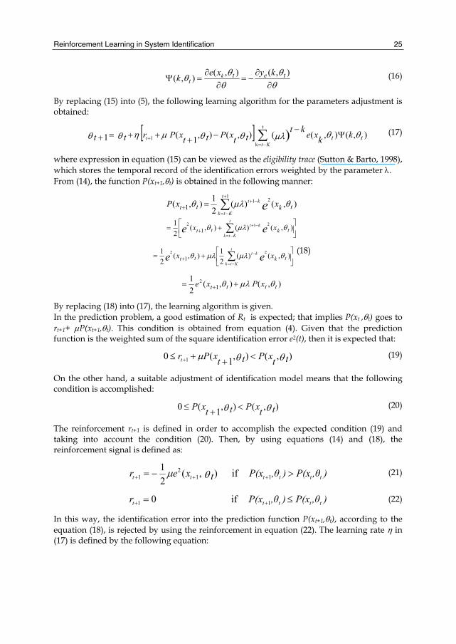
In this case, the unknown function g=[.] is estimated by using the DAFM and, additionally, a sudden change on a(k) is proposed by setting a(k)=0, k>400. After an extensive training phase, the fuzzy model with M=8, δ1=4 and δ2=1 (in equations (8),(9),(11)), has been chosen. In this case, the fuzzy identification performance is adequate and the Root Mean Square Error (RMSE) is 0.1285 in validation phase. Figure 1 shows the performance of the DAFM using the off-line gradient-based tuning algorithm with initial conditions on the interval [0,1] and using the following input signal:

⎩⎨⎧

<<++><<

= 500100 ))25/2(5.0)250/2(5.0(3

500y 1001 )25/2()(

kksenksenkkksen

kuππ

π (30)

Fig. 1. Fuzzy identification using off-line tuning algorithm and DAFM

Reinforcement Learning: Theory and Applications

28

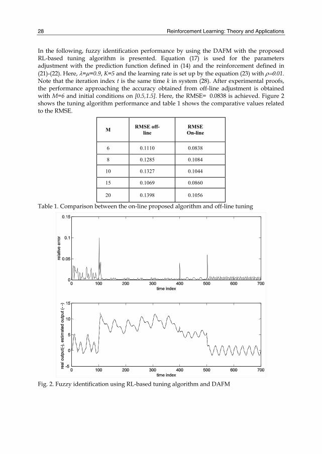
In the following, fuzzy identification performance by using the DAFM with the proposed RL-based tuning algorithm is presented. Equation (17) is used for the parameters adjustment with the prediction function defined in (14) and the reinforcement defined in (21)-(22). Here, λ=μ=0.9, K=5 and the learning rate is set up by the equation (23) with ρ=0.01. Note that the iteration index t is the same time k in system (28). After experimental proofs, the performance approaching the accuracy obtained from off-line adjustment is obtained with M=6 and initial conditions on [0.5,1.5]. Here, the RMSE= 0.0838 is achieved. Figure 2 shows the tuning algorithm performance and table 1 shows the comparative values related to the RMSE.

M RMSE off-line

RMSE On-line

6 0.1110 0.0838

8 0.1285 0.1084

10 0.1327 0.1044

15 0.1069 0.0860

20 0.1398 0.1056

Table 1. Comparison between the on-line proposed algorithm and off-line tuning

Fig. 2. Fuzzy identification using RL-based tuning algorithm and DAFM

Reinforcement Learning in System Identification

29

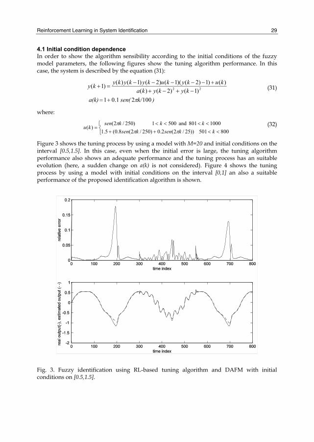
4.1 Initial condition dependence In order to show the algorithm sensibility according to the initial conditions of the fuzzy model parameters, the following figures show the tuning algorithm performance. In this case, the system is described by the equation (31):

)k/ sen(a(k)kykyka

kukykukykykyky

10021.01 )1()2()(

)()1)2()(1()2()1()()1( 22

π+=−+−+

+−−−−−=+ (31)

where:

⎩⎨⎧

<<++<<<<

= 800501 ))25/2(2.0)250/2(8.0(5.1

1000 801 and 5001 )250/2()(

kksenksenkkksen

kuππ

π (32)

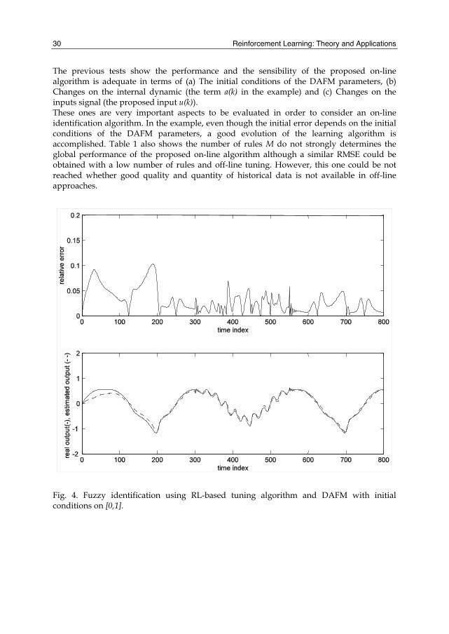
Figure 3 shows the tuning process by using a model with M=20 and initial conditions on the interval [0.5,1.5]. In this case, even when the initial error is large, the tuning algorithm performance also shows an adequate performance and the tuning process has an suitable evolution (here, a sudden change on a(k) is not considered). Figure 4 shows the tuning process by using a model with initial conditions on the interval [0,1] an also a suitable performance of the proposed identification algorithm is shown.

Fig. 3. Fuzzy identification using RL-based tuning algorithm and DAFM with initial conditions on [0.5,1.5].

Reinforcement Learning: Theory and Applications

30

The previous tests show the performance and the sensibility of the proposed on-line algorithm is adequate in terms of (a) The initial conditions of the DAFM parameters, (b) Changes on the internal dynamic (the term a(k) in the example) and (c) Changes on the inputs signal (the proposed input u(k)). These ones are very important aspects to be evaluated in order to consider an on-line identification algorithm. In the example, even though the initial error depends on the initial conditions of the DAFM parameters, a good evolution of the learning algorithm is accomplished. Table 1 also shows the number of rules M do not strongly determines the global performance of the proposed on-line algorithm although a similar RMSE could be obtained with a low number of rules and off-line tuning. However, this one could be not reached whether good quality and quantity of historical data is not available in off-line approaches.

Fig. 4. Fuzzy identification using RL-based tuning algorithm and DAFM with initial conditions on [0,1].

Reinforcement Learning in System Identification

31

5. Acknowledgment This work has been partially presented in the International Symposium on Neural Networks ISNN 2006.

6. Conclusion This work proposes an on-line tuning algorithm based on reinforcement learning for the identification problem. Both the prediction function and the reinforcement signal have been defined by taking into account the identification error, according to the classical recursive identification algorithms. The presence of the reinforcement signal in the proposed tuning algorithm permits to reject the identification error into the prediction function, then, the parameters adjustment not only depends on the gradient direction. The proposed algorithm has been applied in fuzzy identification, then, the prediction function is a non-linear function of the fuzzy model parameters. In this case, the proposed identification model is a Dynamical Adaptive Fuzzy Model (DAFM) that has reported a good performance in identification problems. In order to show the algorithm performance, an illustrative example related to time-varying non-linear system identification using a DAFM has been developed. The obtained results have been compared by using the off-line gradient-based learning algorithm. The performance obtained by using the DAFM with the proposed on-line algorithm is adequate in terms of the main aspects to be taken into account in on-line identification: the initial conditions of the model parameters, the changes on the internal dynamic and the changes on the input signal. Even when similar results could be obtained by using the DAFM with off-line tuning, in this case good quality and quantity of available historical data is needed to reach a suitable validation phase in off-line tuning. This one highlights the use of the on-line learning algorithms and the proposed RL-based on-line tuning algorithm could be an important contribution for the system identification in dynamical environments with perturbations, for example, in process control area.

7. References

Cerrada, M.; Aguilar, J.; Colina, E. & Titli, A. (2002). An approach for dynamical adaptive fuzzy modeling, Proceedings of IEEE-FUZZ 2002 International Conference on Fuzzy Systems, pp. 156-161, Hawai-USA, May 2002, Canada

Cerrada, M.; Aguilar, J.; Colina, E. & Titli, A. (2005). Dynamical membership functions: an approach for adaptive fuzzy modelling. Fuzzy Sets and Systems, Vol. 152, No. 3, (June 2005) (513-533)

Ljung, L. (1997). System Identification. Theory for the User, Prentice Hall, New York Schapire, R.E. & Warmuth, M.K. (1996). On the worst-case analysis of temporal differences

learning algorithms. Machine Learning, Vol. 22, (95-121) Si, J. & Wang, Y-T. (2001). On line learning control by association and reinforcement. IEEE

Transactions on Neural Networks, Vol. 12, No. 2, (264-276)

Reinforcement Learning: Theory and Applications

32

Singh, S.P. & Sutton, R.S. (1996). Reinforcement learning with replacing eligibility traces. Machine Learning, Vol. 22, (123-158)

Sutton, R.S. & Barto, A.G. (1998). Reinforcement Learning. An Introduction, The MIT Press, Cambridge

Sutton, R.S. (1988). Learning to predict by the methods of temporal differences. Machine Learning, Vol. 3, (9-44)

Tesauro, G. (1995). Temporal difference learning and TD-Gammon. Communications of the Association for Computing Machinery, Vol. 38, No. 3, (58-68)

Van Buijtenen, W.M.; Schram, G.; Babuska, R. & Verbruggen, H.B. (1995). Adaptive fuzzy control of satellite attitude by reinforcement learning. IEEE Transactions on Fuzzy Systems, Vol. 6, No. 2, (185-194)

Wang, L.X. (1994). Adaptive Fuzzy Systems and Control, Prentice Hall, New Jersey