HAL Id: tel-03699837https://tel.archives-ouvertes.fr/tel-03699837

Submitted on 20 Jun 2022

HAL is a multi-disciplinary open accessarchive for the deposit and dissemination of sci-entific research documents, whether they are pub-lished or not. The documents may come fromteaching and research institutions in France orabroad, or from public or private research centers.

L’archive ouverte pluridisciplinaire HAL, estdestinée au dépôt et à la diffusion de documentsscientifiques de niveau recherche, publiés ou non,émanant des établissements d’enseignement et derecherche français ou étrangers, des laboratoirespublics ou privés.

Model-based reinforcement learning for dynamicresource allocation in cloud environments

Thomas Tournaire

To cite this version:Thomas Tournaire. Model-based reinforcement learning for dynamic resource allocation in cloud envi-ronments. Computer science. Institut Polytechnique de Paris, 2022. English. �NNT : 2022IPPAS004�.�tel-03699837�

626

NN

T:2

022I

PPA

S004 Model-Based Reinforcement Learning

for Dynamic Resource Allocation inCloud Environments

Thèse de doctorat de l’Institut Polytechnique de Parispréparée à Telecom Sud Paris

École doctorale n◦626 École doctorale de l’Institut Polytechnique deParis (EDIPP)

Spécialité de doctorat : Mathématiques et Informatique

Thèse présentée et soutenue à Paris, le 02Mai 2022, par

Thomas Tournaire

Composition du Jury :

André-Luc BeylotProfesseur, INP ENSEEIHT, Toulouse Président

Nicolas GastCR Inria Grenoble LIG, HDR Rapporteur

Sara AloufCR Inria Sophia-Antipolis NEO, HDR Rapporteure

Tijani ChahedProfesseur, Telecom Sud Paris (SAMOVAR) Examinateur

Bruno TuffinDR Inria Rennes DIONYSOS Examinateur

Sandrine VatonProfesseure, IMTAtlantique Examinatrice

Hind Castel-TalebProfesseure, Telecom Sud Paris (SAMOVAR) Directrice de thèse

Emmanuel HyonMCF, UPL Paris Nanterre) Co-directeur de thèse

Armen AghasaryanIngénieur de recherche et chef d’équipe, Nokia Bell Labs France Invité

ABSTRACT

The emergence of new technologies (Internet of Things, smart cities, autonomous vehicles, health, industrialautomation, ...) requires efficient resource allocation to satisfy the demand. These new offers are compatible withnew 5G network infrastructure since it can provide low latency and reliability. However, these new needs requirehigh computational power to fulfill the demand, implyingmore energy consumption in particular in cloud infra-structures andmore particularly in data centers. Therefore, it is critical to find new solutions that can satisfy theseneeds still reducing the power usage of resources in cloud environments. In this thesis we propose and comparenew AI solutions (Reinforcement Learning) to orchestrate virtual resources in virtual network environmentssuch that performances are guaranteed and operational costs are minimised. We consider queuing systems as amodel for clouds IaaS infrastructures and bring learning methodologies to efficiently allocate the right numberof resources for the users. Our objective is to minimise a cost function considering performance costs and opera-tional costs. We go through different types of reinforcement learning algorithms (from model-free to relationalmodel-based) to learn the best policy. Reinforcement learning is concerned with how a software agent ought totake actions in an environment to maximise some cumulative reward. We first develop queuing model of a cloudsystem with one physical node hosting several virtual resources. On this first part we assume the agent perfectlyknows the model (dynamics of the environment and the cost function), giving him the opportunity to performdynamic programming methods for optimal policy computation. Since the model is known in this part, we alsoconcentrate on the properties of the optimal policies, which are threshold-based and hysteresis-based rules. Thisallows us to integrate the structural property of the policies into MDP algorithms. After providing a concretecloudmodel with exponential arrivals with real intensities and energy data for cloud provider, we compare in thisfirst approach efficiency and time computation ofMDP algorithms against heuristics built on top of the queuingMarkov Chain stationary distributions. In a second part we consider that the agent does not have access to themodel of the environment and concentrate our work with reinforcement learning techniques, especially model-based reinforcement learning.We first developmodel-based reinforcement learningmethods where the agent canre-use its experience replay to update its value function. We also consider MDP online techniques where the au-tonomous agent approximates environment model to perform dynamic programming. This part is evaluated ina larger network environment with two physical nodes in tandem andwe assess convergence time and accuracy ofdifferent reinforcement learning methods, mainly model-based techniques versus the state-of-the-art model-freemethods (e.g. Q-Learning). The last part focuses onmodel-based reinforcement learning techniques with relatio-nal structure between environment variables. As these tandem networks have structural properties due to theirinfrastructure shape, we investigate factored and causal approaches built-in reinforcement learning methods tointegrate this information. We provide the autonomous agent with a relational knowledge of the environmentwhere it canunderstandhowvariables are related to eachother.Themain goal is to accelerate convergence by : firsthaving a more compact representation with factorisation where we devise a factoredMDP online algorithm that

i

we evaluate and compare with model-free and model-based reinforcement learning algorithms; second integra-ting causal and counterfactual reasoning that can tackle environments with partial observations and unobservedconfounders.

Keywords. Reinforcement learning, Markov Decision Process, Queuing systems, Factored reinforcementlearning, Causal reinforcement learning, Auto-scaling policies, Cloud

ii

RÉSUMÉ EN FRANÇAIS

L’émergence de nouvelles technologies nécessite une allocation efficace des ressources pour satisfaire la de-mande. Cependant, ces nouveaux besoins nécessitent une puissance de calcul élevée impliquant une plus grandeconsommation d’énergie notamment dans les infrastructures cloud et data centers. Il est donc essentiel de trou-ver de nouvelles solutions qui peuvent satisfaire ces besoins tout en réduisant la consommation d’énergie desressources. Dans cette thèse, nous proposons et comparons de nouvelles solutions d’IA (apprentissage par ren-forcement RL) pour orchestrer les ressources virtuelles dans les environnements de réseaux virtuels de manièreà garantir les performances et minimiser les coûts opérationnels. Nous considérons les systèmes de file d’attentecomme unmodèle pour les infrastructures cloud IaaS et apportons desméthodes d’apprentissage pour allouer ef-ficacement le bon nombre de ressources. Notre objectif est de minimiser une fonction de coût en tenant comptedes coûts de performance et opérationnels.Nous utilisons différents types d’algorithmes deRL (du« sans-modèle» aumodèle relationnel) pour apprendre la meilleure politique. L’apprentissage par renforcement s’intéresse à lamanière dont un agent doit agir dans un environnement pour maximiser une récompense cumulative. Nous dé-veloppons d’abord un modèle de files d’attente d’un système cloud avec un nœud physique hébergeant plusieursressources virtuelles. Dans cette première partie, nous supposons que l’agent connaît le modèle (dynamiques del’environnement et coût), ce qui lui donne la possibilité d’utiliser des méthodes de programmation dynamiquepour le calcul de la politique optimale. Puisque le modèle est connu dans cette partie, nous nous concentronségalement sur les propriétés des politiques optimales, qui sont des règles basées sur les seuils et l’hystérésis. Celanous permet d’intégrer la propriété structurelle des politiques dans les algorithmes MDP. Après avoir fourni unmodèle de cloud concret avec des arrivées exponentielles avec des intensités réelles et des données d’énergie pourle fournisseur de cloud, nous comparons dans cette première approche l’efficacité et le temps de calcul des algo-rithmes MDP par rapport aux heuristiques construites sur les distributions stationnaires de la chaîne de Markovdes files d’attente. Dans une deuxième partie, nous considérons que l’agent n’a pas accès aumodèle de l’environne-ment et nous concentrons notre travail sur les techniques de RL. Nous évaluons d’abord des méthodes basées surun modèle où l’agent peut réutiliser son expérience pour mettre à jour sa fonction de valeur. Nous considéronségalement des techniques de MDP en ligne où l’agent autonome approxime le modèle pour effectuer une pro-grammation dynamique. Cette partie est évaluée dans un environnement plus large avec deux nœuds physiquesen tandem et nous évaluons le temps de convergence et la précision des différentes méthodes, principalementles techniques basées sur un modèle par rapport aux méthodes sans modèle de l’état de l’art. La dernière partiese concentre sur les techniques de RL basées sur des modèles avec une structure relationnelle entre les variablesd’état. Comme ces réseaux en tandemont des propriétés structurelles dues à la formede l’infrastructure, nous inté-grons les approches factorisées et causales auxméthodes deRL pour inclure cette connaissance. Nous fournissonsà l’agent une connaissance relationnelle de l’environnement qui lui permet de comprendre comment les variablessont reliées. L’objectif principal est d’accélérer la convergence : d’abord avec une représentation plus compacte avec

iii

la factorisation où nous concevons un algorithme en ligne de MDP factorisé que nous comparons avec des algo-rithmes de RL sans modèle et basés sur un modèle ; ensuite en intégrant le raisonnement causal et contrefactuelqui peut traiter les environnements avec des observations partielles et des facteurs de confusion non observés.

Mots-clés. Apprentissage par renforcement, Processus deDécisionsMarkoviens, Files d’attente,Apprentissagepar renforcement factorisé, Apprentissage par renforcement causal, Politiques d’auto-scaling, Cloud

iv

ACKNOWLEDGEMENT

It will be very difficult for me to thank everyone because it is thanks to the help of many people that I was ableto complete this thesis.

First of all, I would like to thank all the members of the Jury (Mr. Andre-Luc Beylot, Mrs. Sandrine Vaton,Mr. Tijani Chahed, Mr. Bruno Tuffin) who participated in the thesis defense, as well as the two reviewers Mrs.Sara Alouf andMr. Nicolas Gast for their detailed reports and their questioning which opened new perspectives.

Iwould also like to thankmy thesis supervisors,Mrs.HindCastel-Taleb andMr. EmmanuelHyon, for all theirhelp, their advice and for all that I could learn at their side. I am delighted to have worked with them because, inaddition to their scientific support, they were always there to support and advise me during the development ofthis thesis.

I also thank my team from Nokia Bell Labs (Armen Aghasaryan, Luka Jakovjlevic, Yue Jin, Makram Bou-zid, Dimitre Kostadinov, Antonio Massaro, Liubov Tupikina) with whom I could learn a lot on many differentsubjects.

I would like to thank the following people for giving me the opportunity to work on several Nokia use-cases :Fahad Syed Muhammad, Veronique Capdevielle, Afef Feki, and also François Durand and Lorenzo Maggi fortheir precious advices in these projects.

I wish to extend my special thanks to Lorenzo Maggi for his kindness, his advices and all the elements i havelearned while working with him.

FInally, I must express my very profound gratitude to my parents Lydie and Bruno, my brother Paul and myFamily for providing me with unfailing support and continuous encouragement throughout my years of studyand through the process of researching and writing this thesis.

Last, I thankmywifeMarie-Annewho has always been present during these three years of thesis, for hermoralsupport, her assistance for the repetition of presentations, and also her sharing of motivation. This accomplish-ment would not have been possible without them.

Thank you.

v

CONTENTS

I Dynamic cloud management 1

1 Introduction 21.1 Motivation . . . . . . . . . . . . . . . . . . . . . . . . . . . . . . . . . . . . . . . . . . . 21.2 Contributions of the thesis . . . . . . . . . . . . . . . . . . . . . . . . . . . . . . . . . . . 41.3 Structure of the thesis . . . . . . . . . . . . . . . . . . . . . . . . . . . . . . . . . . . . . . 6

2 Energy management in Cloud environments 72.1 Cloud systems . . . . . . . . . . . . . . . . . . . . . . . . . . . . . . . . . . . . . . . . . . 7

2.1.1 Definition . . . . . . . . . . . . . . . . . . . . . . . . . . . . . . . . . . . . . . . 72.1.2 Functioning of the Cloud . . . . . . . . . . . . . . . . . . . . . . . . . . . . . . . . 72.1.3 Cloud architectures . . . . . . . . . . . . . . . . . . . . . . . . . . . . . . . . . . . 8

2.2 Energy management . . . . . . . . . . . . . . . . . . . . . . . . . . . . . . . . . . . . . . . 112.2.1 The need for energy management . . . . . . . . . . . . . . . . . . . . . . . . . . . 112.2.2 Measuring and modelling the energy . . . . . . . . . . . . . . . . . . . . . . . . . . 122.2.3 Dynamic resource allocation . . . . . . . . . . . . . . . . . . . . . . . . . . . . . . 13

2.3 Auto-scaling policies . . . . . . . . . . . . . . . . . . . . . . . . . . . . . . . . . . . . . . 142.3.1 Queuing models and control management . . . . . . . . . . . . . . . . . . . . . . . 152.3.2 Threshold-based and hysteresis-based policies . . . . . . . . . . . . . . . . . . . . . 162.3.3 Reinforcement Learning for cloud resource allocation . . . . . . . . . . . . . . . . . 18

3 Reinforcement learning and networking applications 213.1 Markov Decision Process . . . . . . . . . . . . . . . . . . . . . . . . . . . . . . . . . . . . 22

3.1.1 Elements . . . . . . . . . . . . . . . . . . . . . . . . . . . . . . . . . . . . . . . . 223.1.2 Markov Decision Process resolution . . . . . . . . . . . . . . . . . . . . . . . . . . 23

3.2 Reinforcement learning . . . . . . . . . . . . . . . . . . . . . . . . . . . . . . . . . . . . . 263.2.1 Main idea of Reinforcement Learning . . . . . . . . . . . . . . . . . . . . . . . . . 263.2.2 Taxonomy of RL algorithms . . . . . . . . . . . . . . . . . . . . . . . . . . . . . . 283.2.3 Model-free reinforcement learning . . . . . . . . . . . . . . . . . . . . . . . . . . . 293.2.4 Model-based reinforcement learning . . . . . . . . . . . . . . . . . . . . . . . . . . 323.2.5 Reinforcement learning with structural knowledge . . . . . . . . . . . . . . . . . . . 363.2.6 Summary of RL algorithms . . . . . . . . . . . . . . . . . . . . . . . . . . . . . . . 383.2.7 Comparison criteria in reinforcement learning . . . . . . . . . . . . . . . . . . . . . 39

vi

3.3 Model-free or model-based RL? . . . . . . . . . . . . . . . . . . . . . . . . . . . . . . . . . 393.3.1 Industrial networking applications . . . . . . . . . . . . . . . . . . . . . . . . . . . 403.3.2 Thesis position and overview of model-free versus model-based techniques . . . . . . 40

II Model-Based Approaches for Cloud Resource Allocation 42

4 Markov Decision Process or Heuristics : How to compute auto-scaling hysteresis policies in queuing sys-tems with knownmodel 434.1 Introduction . . . . . . . . . . . . . . . . . . . . . . . . . . . . . . . . . . . . . . . . . . 434.2 CloudModel . . . . . . . . . . . . . . . . . . . . . . . . . . . . . . . . . . . . . . . . . . 44

4.2.1 Cloud use-case . . . . . . . . . . . . . . . . . . . . . . . . . . . . . . . . . . . . . 444.2.2 Controlled multi-server queue . . . . . . . . . . . . . . . . . . . . . . . . . . . . . 45

4.3 Hysteresis policies and hysteresis queuing model . . . . . . . . . . . . . . . . . . . . . . . . 464.3.1 Hysteresis policies . . . . . . . . . . . . . . . . . . . . . . . . . . . . . . . . . . . 464.3.2 Hysteresis queuing model and the associatedMarkov chain . . . . . . . . . . . . . . 484.3.3 Cloud provider global cost . . . . . . . . . . . . . . . . . . . . . . . . . . . . . . . 49

4.4 Aggregation methods to compute the global cost . . . . . . . . . . . . . . . . . . . . . . . . 504.4.1 Description of micro-chains and macro-chain . . . . . . . . . . . . . . . . . . . . . 504.4.2 Computation of the mean cost on the aggregated chain . . . . . . . . . . . . . . . . 52

4.5 Heuristics for thresholds calculation using stationary distributions of Markov chain . . . . . . 554.5.1 Local search heuristics . . . . . . . . . . . . . . . . . . . . . . . . . . . . . . . . . 564.5.2 Improvement of local search algorithms with aggregation . . . . . . . . . . . . . . . 574.5.3 Improvement of local search heuristics coupled with initialisation techniques . . . . . 584.5.4 Meta-heuristic approach : the Simulated Annealing (SA) . . . . . . . . . . . . . . . . 634.5.5 Heuristics comparisons : concluding remarks . . . . . . . . . . . . . . . . . . . . . . 65

4.6 Computing policies with Markov Decision Process . . . . . . . . . . . . . . . . . . . . . . . 654.6.1 The SMDPmodel . . . . . . . . . . . . . . . . . . . . . . . . . . . . . . . . . . . 654.6.2 Solving the MDP . . . . . . . . . . . . . . . . . . . . . . . . . . . . . . . . . . . . 684.6.3 Theoretical comparison between the two approaches MC andMDP . . . . . . . . . . 72

4.7 Real model for a Cloud provider . . . . . . . . . . . . . . . . . . . . . . . . . . . . . . . . 744.7.1 Cost-Aware Model with Real Energy Consumption and Pricing . . . . . . . . . . . . 744.7.2 Real Packets traces and CPU utilisation . . . . . . . . . . . . . . . . . . . . . . . . . 75

4.8 Experimental Results . . . . . . . . . . . . . . . . . . . . . . . . . . . . . . . . . . . . . . 754.8.1 Generic experiments to rank the algorithms . . . . . . . . . . . . . . . . . . . . . . 764.8.2 Heuristics vs MDP . . . . . . . . . . . . . . . . . . . . . . . . . . . . . . . . . . . 774.8.3 Numerical experiments for concrete scenarios . . . . . . . . . . . . . . . . . . . . . 79

4.9 Are hysteresis policies really optimal? . . . . . . . . . . . . . . . . . . . . . . . . . . . . . . 834.10 Discussion . . . . . . . . . . . . . . . . . . . . . . . . . . . . . . . . . . . . . . . . . . . . 84

4.10.1 Summary of the chapter . . . . . . . . . . . . . . . . . . . . . . . . . . . . . . . . 844.10.2 How to proceed with unknown statistics . . . . . . . . . . . . . . . . . . . . . . . . 85

5 Model-based Reinforcement Learning for multi-tier network 865.1 BackgroundModel-Based Reinforcement Learning . . . . . . . . . . . . . . . . . . . . . . . 87

5.1.1 Dyna architectures - Deterministic models and buffer replay . . . . . . . . . . . . . . 875.1.2 Real Time Dynamic Programming (RTDP) . . . . . . . . . . . . . . . . . . . . . . 905.1.3 More recent model-based RL techniques . . . . . . . . . . . . . . . . . . . . . . . . 93

vii

5.2 Multi-tier CloudModels . . . . . . . . . . . . . . . . . . . . . . . . . . . . . . . . . . . . 945.2.1 TandemQueue : Environment 1 . . . . . . . . . . . . . . . . . . . . . . . . . . . . 945.2.2 Semi Markov Decision Process Description . . . . . . . . . . . . . . . . . . . . . . . 955.2.3 MMPP TandemQueue model : Environment 2 . . . . . . . . . . . . . . . . . . . . 975.2.4 Simulated SMDP environment and objective function for RL agent . . . . . . . . . . 99

5.3 Generalisation and Selection of Model-based Reinforcement Learning Algorithms . . . . . . . 995.3.1 Algorithms selection . . . . . . . . . . . . . . . . . . . . . . . . . . . . . . . . . . 1005.3.2 Learning process . . . . . . . . . . . . . . . . . . . . . . . . . . . . . . . . . . . . 1005.3.3 Planning process . . . . . . . . . . . . . . . . . . . . . . . . . . . . . . . . . . . . 1005.3.4 Integration planning and learning . . . . . . . . . . . . . . . . . . . . . . . . . . . 1005.3.5 Parameters of model-based RL techniques . . . . . . . . . . . . . . . . . . . . . . . 101

5.4 Experimental Results . . . . . . . . . . . . . . . . . . . . . . . . . . . . . . . . . . . . . . 1015.4.1 Comparison Criteria between RL Algorithms . . . . . . . . . . . . . . . . . . . . . 1035.4.2 Simulation Environment and Parameters . . . . . . . . . . . . . . . . . . . . . . . . 1035.4.3 Experimental Results for Initial TandemQueue Environment . . . . . . . . . . . . . 1055.4.4 Experimental Results for MMPP TandemQueue . . . . . . . . . . . . . . . . . . . 1075.4.5 Final comparison in two multi-tier environments . . . . . . . . . . . . . . . . . . . 107

5.5 Summary of the chapter . . . . . . . . . . . . . . . . . . . . . . . . . . . . . . . . . . . . . 108

III Model-Based Reinforcement Learning with Relational Structure between Environ-ment Variables 110

6 Factored reinforcement learning for multi-tier network 1116.1 Background . . . . . . . . . . . . . . . . . . . . . . . . . . . . . . . . . . . . . . . . . . . 112

6.1.1 Coffee Robot Example : Illustration for the factored framework . . . . . . . . . . . . 1126.1.2 Formalism . . . . . . . . . . . . . . . . . . . . . . . . . . . . . . . . . . . . . . . 1136.1.3 FactoredMDPmethodologies . . . . . . . . . . . . . . . . . . . . . . . . . . . . . 1156.1.4 Factored Reinforcement Learning . . . . . . . . . . . . . . . . . . . . . . . . . . . 1196.1.5 Feasibility study of FVI in the Coffee Robot Problem . . . . . . . . . . . . . . . . . 121

6.2 FactoredModel-Based Reinforcement Learning . . . . . . . . . . . . . . . . . . . . . . . . . 1216.2.1 Factored probabilities inference . . . . . . . . . . . . . . . . . . . . . . . . . . . . . 1226.2.2 Factored planning . . . . . . . . . . . . . . . . . . . . . . . . . . . . . . . . . . . 1226.2.3 Exploration-Exploitation trade-off . . . . . . . . . . . . . . . . . . . . . . . . . . . 1226.2.4 Inputs and parameters . . . . . . . . . . . . . . . . . . . . . . . . . . . . . . . . . 122

6.3 FactoredMDP representation of the TandemQueue Environment . . . . . . . . . . . . . . . 1236.3.1 Factored model representation . . . . . . . . . . . . . . . . . . . . . . . . . . . . . 1236.3.2 FactoredMDPmodel with Augmented State Space . . . . . . . . . . . . . . . . . . 1256.3.3 Objective function . . . . . . . . . . . . . . . . . . . . . . . . . . . . . . . . . . . 1276.3.4 Parameters selection of FMDP online . . . . . . . . . . . . . . . . . . . . . . . . . 127

6.4 Numerical Results . . . . . . . . . . . . . . . . . . . . . . . . . . . . . . . . . . . . . . . . 1286.4.1 Environments and Simulation Parameters . . . . . . . . . . . . . . . . . . . . . . . 1286.4.2 Comparison Criteria between Algorithms . . . . . . . . . . . . . . . . . . . . . . . 1286.4.3 Results . . . . . . . . . . . . . . . . . . . . . . . . . . . . . . . . . . . . . . . . . 129

6.5 Summary of the chapter . . . . . . . . . . . . . . . . . . . . . . . . . . . . . . . . . . . . . 131

viii

7 Causal reinforcement learning for multi-tier network 1327.1 Introduction to causality : Pearl’s Causal Hierarchy . . . . . . . . . . . . . . . . . . . . . . . 133

7.1.1 Layer 1 - Observational . . . . . . . . . . . . . . . . . . . . . . . . . . . . . . . . . 1337.1.2 Layer 2 - Interventional . . . . . . . . . . . . . . . . . . . . . . . . . . . . . . . . . 1347.1.3 Layer 3 - Counterfactual : the imaginary world . . . . . . . . . . . . . . . . . . . . . 1347.1.4 Why reinforcement learning can suffer for policy optimisation . . . . . . . . . . . . . 136

7.2 Causal Reinforcement Learning : Formalism and Environments . . . . . . . . . . . . . . . . 1387.2.1 Causal Reinforcement Learning literature . . . . . . . . . . . . . . . . . . . . . . . 1387.2.2 Markov decision process environment’s representation . . . . . . . . . . . . . . . . . 1397.2.3 MDP Environments . . . . . . . . . . . . . . . . . . . . . . . . . . . . . . . . . . 1397.2.4 SCM representation of MDP environments . . . . . . . . . . . . . . . . . . . . . . 1427.2.5 Counterfactual reasoning inMDP environments . . . . . . . . . . . . . . . . . . . . 144

7.3 Causal modelling of multi-tier Cloud architectures . . . . . . . . . . . . . . . . . . . . . . . 1497.3.1 EnvA1 Tandem queueMDPmodel . . . . . . . . . . . . . . . . . . . . . . . . . . 1507.3.2 Env C1 Tandem queueMDPUC environment . . . . . . . . . . . . . . . . . . . . . 153

7.4 Experimental results . . . . . . . . . . . . . . . . . . . . . . . . . . . . . . . . . . . . . . . 1577.4.1 Environments and Simulation Parameters . . . . . . . . . . . . . . . . . . . . . . . 1587.4.2 EnvA1 Tandem queueMDP environment . . . . . . . . . . . . . . . . . . . . . . 1587.4.3 Env C1 Tandem queueMDPUC environment . . . . . . . . . . . . . . . . . . . . . 158

7.5 Summary of the chapter . . . . . . . . . . . . . . . . . . . . . . . . . . . . . . . . . . . . . 159

8 Discussion 1608.1 Taxonomy of the Reinforcement Learning field . . . . . . . . . . . . . . . . . . . . . . . . . 1608.2 Conclusion of the thesis . . . . . . . . . . . . . . . . . . . . . . . . . . . . . . . . . . . . . 1628.3 Perspectives of the thesis . . . . . . . . . . . . . . . . . . . . . . . . . . . . . . . . . . . . . 163

A Appendix 176A.1 Stationary distributions of classical queues . . . . . . . . . . . . . . . . . . . . . . . . . . . 176

A.1.1 Computation of the stationary distribution . . . . . . . . . . . . . . . . . . . . . . 177

ix

LIST OF TABLES

4.1 Summary of algorithms based onMarkov chain stationary distribution computation . . . . . 654.2 Numerical experiments for comparison of heuristics andMDP algorithm . . . . . . . . . . . 784.3 High-scale datacenter resolution withMDP algorithmHy-PI . . . . . . . . . . . . . . . . . 794.4 Parameter values for three scenarios . . . . . . . . . . . . . . . . . . . . . . . . . . . . . . . 804.5 Policy q(m, k) returned by Value Iteration showing non-hysteresis . . . . . . . . . . . . . . . 84

5.1 Summary of selected model-based RL algorithms . . . . . . . . . . . . . . . . . . . . . . . . 1015.2 Average discounted reward obtained by a Monte Carlo policy evaluation after a fix period of

learning . . . . . . . . . . . . . . . . . . . . . . . . . . . . . . . . . . . . . . . . . . . . . 107

6.1 CPT of local variable sC under actionDelC . . . . . . . . . . . . . . . . . . . . . . . . . . 1146.2 Tabular representation of the reward function in the Coffee Robot . . . . . . . . . . . . . . . 1146.3 Policies and value functions returned by VI and FVI for some Coffee Robot states . . . . . . . 1216.4 Child-parent architecture . . . . . . . . . . . . . . . . . . . . . . . . . . . . . . . . . . . . 1236.5 Basis functions selection for factored value iteration . . . . . . . . . . . . . . . . . . . . . . . 127

8.1 Categorisation of reinforcement learning algorithms . . . . . . . . . . . . . . . . . . . . . . 162

x

LIST OF FIGURES

1.1 Principal type of networks considered in the thesis . . . . . . . . . . . . . . . . . . . . . . . 31.2 Thesis flow chart . . . . . . . . . . . . . . . . . . . . . . . . . . . . . . . . . . . . . . . . 6

2.1 Different Cloud Service Models . . . . . . . . . . . . . . . . . . . . . . . . . . . . . . . . . 92.2 Virtualisation process with VMs and containers . . . . . . . . . . . . . . . . . . . . . . . . . 102.3 Three tier architecture . . . . . . . . . . . . . . . . . . . . . . . . . . . . . . . . . . . . . . 102.4 Increase in data usage and Cloud . . . . . . . . . . . . . . . . . . . . . . . . . . . . . . . . 11

3.1 RL interaction between an agent and the environment (Figure from [46]) . . . . . . . . . . . 213.2 Two principal differences between reinforcement learning methods . . . . . . . . . . . . . . . 293.3 Breadth and Depth for a planning iteration (Figure from [106]) - The red dot line excludes the

exhaustive search unfeasible in MDP environments . . . . . . . . . . . . . . . . . . . . . . . 363.4 Reichenbach’s principle . . . . . . . . . . . . . . . . . . . . . . . . . . . . . . . . . . . . . 373.5 Causal Reinforcement Learning : How can each field help the other (Figure from [96]) . . . . 383.6 Taxonomy of reinforcement learning methods and their application in the thesis . . . . . . . . 39

4.1 Representation of a Cloud Architecture . . . . . . . . . . . . . . . . . . . . . . . . . . . . . 454.2 Multi-server queuing system . . . . . . . . . . . . . . . . . . . . . . . . . . . . . . . . . . 464.3 An isotone hysteresis policy. . . . . . . . . . . . . . . . . . . . . . . . . . . . . . . . . . . . 474.4 The hysteresis queuing model . . . . . . . . . . . . . . . . . . . . . . . . . . . . . . . . . . 494.5 Example with K=3 VMs and B maximum requests in the system . . . . . . . . . . . . . . . . 504.6 Example of micro-chains fromMarkov Chain of Fig.4.5 . . . . . . . . . . . . . . . . . . . . 514.7 TheMacro chain . . . . . . . . . . . . . . . . . . . . . . . . . . . . . . . . . . . . . . . . 514.8 Example of an isotone hysteresis multichain MDP . . . . . . . . . . . . . . . . . . . . . . . 694.9 Temporal behavior for the Markov chain approach . . . . . . . . . . . . . . . . . . . . . . . 734.10 Temporal behavior for the MDP approach . . . . . . . . . . . . . . . . . . . . . . . . . . . 734.11 Comparison of accuracy and time execution between heuristics . . . . . . . . . . . . . . . . . 764.12 Energy and performance costs given fixed SLA or arrival rate . . . . . . . . . . . . . . . . . . 824.13 Financial Cost for an hour depending on the SLA . . . . . . . . . . . . . . . . . . . . . . . . 824.14 Financial Cost for an hour depending on the workload . . . . . . . . . . . . . . . . . . . . . 83

5.1 The reinforcement learning scheme in Dyna architectures (Figure from [8]) . . . . . . . . . . 875.2 Tandem queue representation of three-tier architecture . . . . . . . . . . . . . . . . . . . . . 955.3 Average reward over learning episodes in tandem queue environment with larger scale . . . . . 105

xi

5.4 C1 average discounted reward obtained by RL algorithms . . . . . . . . . . . . . . . . . . . . 1065.5 C2 average discounted reward obtained by RL algorithms . . . . . . . . . . . . . . . . . . . 1065.6 C3 average discounted reward obtained by RL algorithms . . . . . . . . . . . . . . . . . . . 1065.7 Comparison of RL algorithms in two tandem queue environments . . . . . . . . . . . . . . . 108

6.1 Example of the DBN under actionDelC in the Coffee Robot . . . . . . . . . . . . . . . . . 1136.2 Representation of the reward functionR in the Coffee Robot . . . . . . . . . . . . . . . . . 1146.3 Tree representation for the CPT of variable sC under actionDelC . . . . . . . . . . . . . . . 1166.4 Comparison of the representation of a function f as a decision tree Tree [f] (a) and as an algebraic

decision diagram ADD[f] (b) ; Figure from [2] . . . . . . . . . . . . . . . . . . . . . . . . . 1176.5 Dynamic Bayesian Networks under any action a for original tandem queueMDP . . . . . . . 1246.6 Correlation between state variables after 20000 samples collected by RL agent . . . . . . . . . 1256.7 Dynamic Bayesian Network representation for factored tandem queueMDP . . . . . . . . . 1256.8 Action a1 = −1 . . . . . . . . . . . . . . . . . . . . . . . . . . . . . . . . . . . . . . . . . 1266.9 Action a1 = 0 . . . . . . . . . . . . . . . . . . . . . . . . . . . . . . . . . . . . . . . . . . 1266.10 Action a1 = 1 . . . . . . . . . . . . . . . . . . . . . . . . . . . . . . . . . . . . . . . . . . 1266.11 Factored probabilities for variable k1 under all actions a1 . . . . . . . . . . . . . . . . . . . . 1266.12 Average reward per episode over learning episodes in cloudC1 . . . . . . . . . . . . . . . . . 1296.13 Average reward per episode over learning episodes in cloudC2 . . . . . . . . . . . . . . . . . 1306.14 Barplots showing running time of model-based RL algorithms . . . . . . . . . . . . . . . . . 130

7.1 Pearl’s causal hierarchy representation of the world (Figure from [20] . . . . . . . . . . . . . . 1337.2 Summary of the three causal layers [20] . . . . . . . . . . . . . . . . . . . . . . . . . . . . . 1357.3 Recovery rate for patients in kidney stone example . . . . . . . . . . . . . . . . . . . . . . . 1367.4 Two different representations of the environment dynamics . . . . . . . . . . . . . . . . . . 1407.5 Partially observable MDP transition from t to t+ 1 (Figure from [2]) . . . . . . . . . . . . . 1417.6 Temporal causal graph for toy example . . . . . . . . . . . . . . . . . . . . . . . . . . . . . 1447.7 Temporal causal graph for toy example with partial observation . . . . . . . . . . . . . . . . 1477.8 Temporal causal graph for toy example with unobserved confounder . . . . . . . . . . . . . . 1487.9 Tandem queue temporal causal graph . . . . . . . . . . . . . . . . . . . . . . . . . . . . . . 1507.10 Tandem queue temporal causal graph under intervention . . . . . . . . . . . . . . . . . . . . 1517.11 Environment behavior under physician’s policy q . . . . . . . . . . . . . . . . . . . . . . . . 1537.12 Environment behavior under the learning agent’s decisions . . . . . . . . . . . . . . . . . . . 1547.13 Environment behavior under the learning agent’s decisions with the extended observation . . . 1547.14 Cumulative reward obtained by different algorithms over learning episodes . . . . . . . . . . . 1557.15 Average reward obtained by different algorithms over learning episodes . . . . . . . . . . . . . 1557.16 MDPUC Tandem queue temporal causal graph . . . . . . . . . . . . . . . . . . . . . . . . . 1567.17 MDPUC Tandem queue temporal causal graph under intervention . . . . . . . . . . . . . . 1577.18 Average reward over learning episodes between RL algorithms inMDP scenario . . . . . . . . 1587.19 Average reward over learning episodes between RL algorithms inMDPUC scenario . . . . . . 159

8.1 Ladder of representation for environments dynamics . . . . . . . . . . . . . . . . . . . . . . 161

xii

LIST OF ALGORITHMS

1 Value Iteration - Discounted criteria . . . . . . . . . . . . . . . . . . . . . . . . . . . . . . . 252 Policy Iteration - Discounted criteria . . . . . . . . . . . . . . . . . . . . . . . . . . . . . . . 253 Relative Value Iteration - Average criteria . . . . . . . . . . . . . . . . . . . . . . . . . . . . . 264 TD(0)-Learning - Discounted criteria . . . . . . . . . . . . . . . . . . . . . . . . . . . . . . 285 Q-Learning . . . . . . . . . . . . . . . . . . . . . . . . . . . . . . . . . . . . . . . . . . . . 306 Deep-Q-Network . . . . . . . . . . . . . . . . . . . . . . . . . . . . . . . . . . . . . . . . . 317 REINFORCE : a policy-based algorithm . . . . . . . . . . . . . . . . . . . . . . . . . . . . . 32

8 First aggregated cost computation : FACC . . . . . . . . . . . . . . . . . . . . . . . . . . . . 549 Calculation of the cost for the current solution after changes in Fl orRl : CACC . . . . . . . . 5510 Best per Level . . . . . . . . . . . . . . . . . . . . . . . . . . . . . . . . . . . . . . . . . . . 5611 Increasing . . . . . . . . . . . . . . . . . . . . . . . . . . . . . . . . . . . . . . . . . . . . . 5712 Neighbour Local Search . . . . . . . . . . . . . . . . . . . . . . . . . . . . . . . . . . . . . 5713 Best per Level coupled with cost aggregation . . . . . . . . . . . . . . . . . . . . . . . . . . . 5814 Fluid approximation . . . . . . . . . . . . . . . . . . . . . . . . . . . . . . . . . . . . . . . 6015 Neighbour Local Search with Fluid approximation initialisation . . . . . . . . . . . . . . . . . 6016 MMK approximation . . . . . . . . . . . . . . . . . . . . . . . . . . . . . . . . . . . . . . . 6217 Neighbour Local Search . . . . . . . . . . . . . . . . . . . . . . . . . . . . . . . . . . . . . 6318 Simulated Annealing . . . . . . . . . . . . . . . . . . . . . . . . . . . . . . . . . . . . . . . 6419 Policy Iteration with double level properties pseudo-code . . . . . . . . . . . . . . . . . . . . 7120 Policy Iteration with hysteresis properties pseudo-code . . . . . . . . . . . . . . . . . . . . . . 71

21 Dyna-Q Algorithm [8] . . . . . . . . . . . . . . . . . . . . . . . . . . . . . . . . . . . . . . 8822 Dyna-Q-+ Algorithm [8] . . . . . . . . . . . . . . . . . . . . . . . . . . . . . . . . . . . . . 8923 Dyna-Q-prior Algorithm [8] . . . . . . . . . . . . . . . . . . . . . . . . . . . . . . . . . . . 9024 E3 - PAC-MDP Algorithm [74] . . . . . . . . . . . . . . . . . . . . . . . . . . . . . . . . . . 9225 R-max - PAC-MDP Algorithm [27] . . . . . . . . . . . . . . . . . . . . . . . . . . . . . . . 9326 Model-based RL with model approximations at a given episode t [115] . . . . . . . . . . . . . 9427 Generalised Model-based reinforcement learning . . . . . . . . . . . . . . . . . . . . . . . . . 102

28 Factored Value Iteration . . . . . . . . . . . . . . . . . . . . . . . . . . . . . . . . . . . . . 11929 FactoredMDP online algorithm . . . . . . . . . . . . . . . . . . . . . . . . . . . . . . . . . 123

30 Counterfactual-based data augmentation RL (CDYNA - Causal Dyna-Q-Learning) . . . . . . 146

xiii

31 Causal policy-based reinforcement learning for POMDP [30] . . . . . . . . . . . . . . . . . . 148

32 Markov chain resolution with GTH . . . . . . . . . . . . . . . . . . . . . . . . . . . . . . . 17733 The power method . . . . . . . . . . . . . . . . . . . . . . . . . . . . . . . . . . . . . . . . 17834 Renormalise(x) : Renormalisation of a vector . . . . . . . . . . . . . . . . . . . . . . . . . . . 178

xiv

NOMENCLATURE

Queuing systems

λ Arrival rate in queuing systems

µ Service rate in queuing systems

Π Stationary distribution of the macro chain

π Markov Chain stationary distribution

πk Stationary distribution of a micro chain of level k

Bi Maximum number of requests in the buffer of physical node i

CA Cost of activating one VM

CD Cost of deactivating one VM

CH Cost of holding for requests in system within 1 time unit

CR Cost of rejecting one request due to full queue

CS Cost of one working VMwithin one time unit

Fk Number of requests such that we activate a VM

K Total number of virtual resources (VMs) in physical node i

ki Number of activated virtual resources in physical node i

mi Number of jobs in physical node i

q Control policy

Rk Number of requests such that we deactivate a VM

Reinforcement Learning

P Uniformised probability distribution

R Uniformised reward function

A Action space

P Probability transition

xv

Q Action-value function

R Reward function

S State space

V State-value function

P Approximated probability distribution

R Approximated reward function

q Policy

xvi

PART I

DYNAMIC CLOUDMANAGEMENT

1

CHAPTER 1

INTRODUCTION

1.1 MotivationThe emergence of new technologies (Internet of Things IoT, smart cities, autonomous vehicles, health, indus-

trial automation, augmented reality, ...) requires a growing need for network and cloud to satisfy low latency andreliability. These emerging technologies will increase the resource requirements by requiring high computationalpower and therefore the energy consumption of the networks. This phenomenon is receiving a lot of attentionfrom the world’s governments regarding the need to reduce the energy consumption of the cloud. Indeed, thetheme of energy-efficient cloud computing is now a priority on the European Union (EU) political agenda. In2018, the energy consumption of data centers in the EU was 76.8 TWh and is expected to rise to 98,52 TWhby 2030, a 28% increase. In addition, the Information and Communication Technology (ICT) sector is a majorenergy consumer, using about 4% of the world’s electricity today and expected to account for 10-20% of globalelectricity consumption by 2030. Also, the global digital ecosystem is responsible for 2% to 4% of the world’sgreenhouse gas emissions, up to twice as much as air travel 1.

There is therefore anurgentneed to find intelligent resource allocationpolicies that can reduce energy consump-tion and satisfy modern and future needs. Queuing theory is a branch of mathematics that studies how queuesform, how they work and why they don’t work. It looks at every component of waiting in line, including thearrival process, the service process, the number of servers, the number of seats in the system, and the numberof customers - which can be people, data packets, cars, etc. Queuing theory is often used to represent, analyseand optimise Cloud systems, by representing such infrastructures with multiple nodes (physical servers, virtualresources, etc.) in network. Cloud infrastructures are physical nodes hosting virtual resources, connected in a net-work. Figure 1.1 is a very small representation of such systems where User’s Equipments (UEs) send requests to beprocessed by the Cloud and asking for a response. The queuingmodels allow researchers to evaluate performancemetrics such as number of requests (or customers), delays, losses, CPU utilisation rate, energy consumption, etc.

Abstracting cloud infrastructures and networks with queuing models allows us to devise and assess new in-telligent algorithms by evaluating their performance. The main objective of this thesis is to provide and assessalgorithms based on artificial intelligence (AI) that can learn and update efficient policies continuously for re-source allocation. These learned policies (or solutions) are rules that tell the agent what decision to make for anobservation of the cloud system. Activation and deactivation of resources (virtual or physical) is an indispensablepart of energy management and our goal is therefore to consider such activation/deactivation rules in Cloud sys-

1. Guillaume Pitron, L’enfer numérique - voyage au bout d’un like, Les Liens Qui Liberent, 2021

2

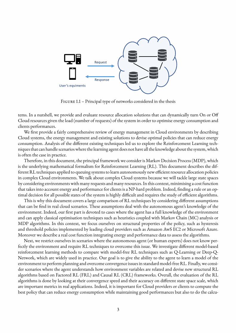
Figure 1.1 – Principal type of networks considered in the thesis

tems. In a nutshell, we provide and evaluate resource allocation solutions that can dynamically turn On or OffCloud resources given the load (number of requests) of the system in order to optimise energy consumption andclients performances.

We first provide a fairly comprehensive review of energy management in Cloud environments by describingCloud systems, the energy management and existing solutions to devise optimal policies that can reduce energyconsumption. Analysis of the different existing techniques led us to explore the Reinforcement Learning tech-niques that canhandle scenarioswhere the learning agent does not have all the knowledge about the system,whichis often the case in practice.

Therefore, in this document, the principal framework we consider isMarkovDecision Process (MDP), whichis the underlying mathematical formalism for Reinforcement Learning (RL). This document describes the dif-ferentRL techniques applied to queuing systems to learn autonomously new efficient resource allocation policiesin complex Cloud environments. We talk about complex Cloud systems because we will tackle large state spacesby considering environments withmany requests andmany resources. In this context,minimising a cost functionthat takes into account energy and performance for clients is a NP-hard problem. Indeed, finding a rule or an op-timal decision for all possible states of the system is highly difficult and requires the study of efficient algorithms.

This is why this document covers a large comparison of RL techniques by considering different assumptionsthat can be find in real cloud scenarios. These assumptions deal with the autonomous agent’s knowledge of theenvironment. Indeed, our first part is devoted to cases where the agent has a full knowledge of the environmentand can apply classical optimisation techniques such as heuristics coupled with Markov Chain (MC) analysis orMDP algorithms. In this context, we focus ourselves on structural properties of the policy, such as hysteresisand threshold policies implemented by leading cloud providers such as Amazon AwS EC2 or Microsoft Azure.Moreover we describe a real cost function integrating energy and performance data to assess the algorithms.

Next, we restrict ourselves in scenarios where the autonomous agent (or human experts) does not know per-fectly the environment and require RL techniques to overcome this issue. We investigate different model-basedreinforcement learning methods to compare with model-free RL techniques such as Q-Learning or Deep-Q-Network, which are widely used in practice. Our goal is to give the ability to the agent to learn a model of theenvironment to performplanning and overcome convergence issues in standardmodel-freeRL. Finally, we consi-der scenarios where the agent understands how environment variables are related and devise new structural RLalgorithms based on Factored RL (FRL) and Causal RL (CRL) frameworks. Overall, the evaluation of the RLalgorithms is done by looking at their convergence speed and their accuracy on different state space scale, whichare important metrics in real applications. Indeed, it is important for Cloud providers or clients to compute thebest policy that can reduce energy consumption while maintaining good performances but also to do the calcu-

3

lation rapidly to cope with fast changing environments. Thus the comparison of RL methods is done based onthese two elements : accuracy and convergence speed.

For short, this thesis includes two major components : searching for auto-scaling solutions in cloud networksystems and building more efficient RL/AI algorithms. We have explored and searched among many techniquesthat allow to go beyond the classical state-of-the-art (SoTA) RL and they are described in this document. Thisresearch is divided in twomain axes which are located in two parts : model-based RL and structural model-basedRL.

1.2 Contributions of the thesisThe contributions of this thesis are as follows :

∗ Chapter II presents an overview of state of the art (SoTA) techniques for Cloud network modelling, Cloudauto-scaling, Cloud energy management and optimisation with machine learning techniques.∗ Chapter III introduces the formalismof reinforcement learning anddiscussmany state of the art techniques.This review of the reinforcement learning literature was assisted by concrete studies in the network field,mainly with model-free RL techniques. These studies were conducted at Nokia Bell Labs and allowed meto work on two patents.∗ F. SyedMuhammad, R. Damodaran, T. Tournaire, A. Feki, L. Maggi, F. Durand, U. Chowta.AI/ML based PDCP Split in Dual/Multi Connectivity Configurations : CollectiveInference/Decision and Impact on 3gpp Interfaces, Nokia, 2021.∗ T. Tournaire, F. SyedMuhammad, A. Feki, L. Maggi, F. Durand.Multi-Agent ReinforcementLearning Sharing Common Neural Network Policy for PDCP Data Split, Nokia, 2021.

ThePart II of the thesis dealswithmodel-based reinforcement learning domain for computing and learningauto-scaling policies in Cloud environments :∗ Chapter IV is about auto-scaling threshold policies in Cloud systems when the agent knows the environ-ment model. It studies and compares two mathematical approach to find optimal threshold policies in aCloud environment, modelled withmulti-server queuing systems : Heuristics based on the computation ofstationary distribution of the Markov chain and Markov Decision Process. It compares many local searchheuristics and proposes many improvement techniques : Initialisation of the heuristics, Aggregation tech-nique for fast cost computation;Meta-heuristic. Next, it studies meticulously theMarkovDecision Processapproach and designs new Dynamic Programming algorithms integrating the structure of the policy, na-mely hysteresis and thresholds properties. Finally it proposes a real cloud scenariowhich features real energy,financial data and requests arrivals. All techniques are compared numerically.This chapter has led to two publications [139, 141] :∗ Thomas Tournaire, Hind Castel-Taleb, Emmanuel Hyon. Generating optimal thresholds in a hysteresisqueue : a cloud application. In 27th IEEE International Symposium on the Modeling, Analysis, and Simu-lation of Computer and Telecommunication Systems (MASCOTS 19), 2019.∗ Thomas Tournaire, Hind Castel-Taleb, Emmanuel Hyon. Optimal control policies for resource alloca-tion in the Cloud : comparison between Markov decision process and heuristic approaches. In CoRRabs/2104.14879, 2021.

4

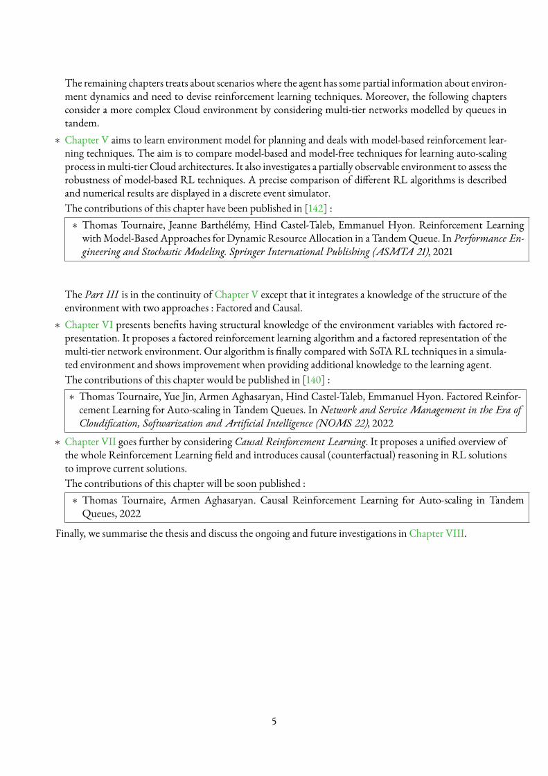
The remaining chapters treats about scenarios where the agent has some partial information about environ-ment dynamics and need to devise reinforcement learning techniques. Moreover, the following chaptersconsider a more complex Cloud environment by considering multi-tier networks modelled by queues intandem.∗ Chapter V aims to learn environment model for planning and deals with model-based reinforcement lear-ning techniques. The aim is to compare model-based and model-free techniques for learning auto-scalingprocess inmulti-tier Cloud architectures. It also investigates a partially observable environment to assess therobustness of model-based RL techniques. A precise comparison of different RL algorithms is describedand numerical results are displayed in a discrete event simulator.The contributions of this chapter have been published in [142] :∗ Thomas Tournaire, Jeanne Barthélémy, Hind Castel-Taleb, Emmanuel Hyon. Reinforcement LearningwithModel-Based Approaches for Dynamic Resource Allocation in a TandemQueue. In Performance En-gineering and Stochastic Modeling. Springer International Publishing (ASMTA 21), 2021

The Part III is in the continuity of Chapter V except that it integrates a knowledge of the structure of theenvironment with two approaches : Factored and Causal.∗ Chapter VI presents benefits having structural knowledge of the environment variables with factored re-presentation. It proposes a factored reinforcement learning algorithm and a factored representation of themulti-tier network environment. Our algorithm is finally compared with SoTARL techniques in a simula-ted environment and shows improvement when providing additional knowledge to the learning agent.The contributions of this chapter would be published in [140] :∗ Thomas Tournaire, Yue Jin, Armen Aghasaryan, Hind Castel-Taleb, Emmanuel Hyon. Factored Reinfor-cement Learning for Auto-scaling in TandemQueues. InNetwork and Service Management in the Era ofCloudification, Softwarization and Artificial Intelligence (NOMS 22), 2022

∗ Chapter VII goes further by considering Causal Reinforcement Learning. It proposes a unified overview ofthe whole Reinforcement Learning field and introduces causal (counterfactual) reasoning in RL solutionsto improve current solutions.The contributions of this chapter will be soon published :∗ Thomas Tournaire, Armen Aghasaryan. Causal Reinforcement Learning for Auto-scaling in TandemQueues, 2022

Finally, we summarise the thesis and discuss the ongoing and future investigations in Chapter VIII.

5

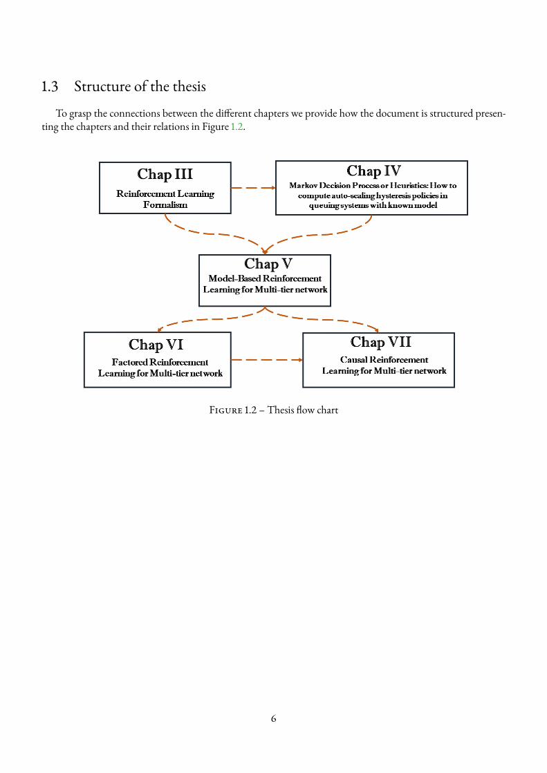
1.3 Structure of the thesisTo grasp the connections between the different chapters we provide how the document is structured presen-

ting the chapters and their relations in Figure 1.2.

Figure 1.2 – Thesis flow chart

6

CHAPTER 2

ENERGYMANAGEMENT IN CLOUD ENVIRONMENTS

This chapter presents literature works about Cloud computing, energy management, queuing models, andoptimisation techniques for resource allocation. It first presents what is Cloud computing, how it behaves, theexisting infrastructures and models (e.g. datacenter) and the virtualisation framework (section 2.1). Next it givesan overview of energy management field by presenting the need, the solutions to measure and model, and dy-namic resource allocation paradigm (section 2.2). Finally, it presents the existing auto-scaling techniques withthresholds-based rules, queuing models and control management and reinforcement learning techniques (sec-tion 2.3).

2.1 Cloud systems

2.1.1 DefinitionCloud Computing is a recent technology that allows access to data or infrastructure using an internet connec-

tion. This data is managed remotely by physical or virtual servers installed in a datacenter. This online storagespace would go back, according to the newspaper 1 to the 1990’s and the name Cloud would have been born in2006 with the former CEO of Google, Eric Schmidt. Today, many companies have invested massively in CloudComputing. Among the main companies of the sector are Amazon (AwS), Citrix, Google, IBM, Intel, MicrosoftorOVHcloud. Users can then subscribe to different Cloud services, such as AmazonDrive, GoogleDrive,Micro-soft OneDrive or formore professional applications withMicrosoft Sharepoint for example and any applicationsto store companies data. In 2018 it was estimated that 3.6 billion people were accessing a huge range of cloudcomputing services.

2.1.2 Functioning of the CloudIn order to operate, a Cloud needs to have several essential characteristics :∗ The implementation of the systems is entirely automated and the customer can, according to the contractsigned with the owner of the Cloud, have access thanks to the network to software or to his data when hewishes it and from anywhere in the world.

1. Technology Review

7

∗ Broadband network access : The datacenters that host these Clouds are generally connected directly to theInternet backbone (very powerful Internet network) to have excellent connectivity. The large providers thendistribute different processing centers around the world to provide very fast access to systems for peoplearound the world.∗ Resource Reservoir : Most data centers contain tens of thousands of servers and storage facilities to allowfor rapid scalability.∗ Rapid scaling (elasticity) : Bringing a new server instance online is done in minutes, shutting down andrestarting in seconds. These management techniques allow you to take full advantage of pay-per-use billingby adapting computing power to instantaneous traffic.∗ The use of resources can be monitored and controlled, which makes it possible to optimize resource alloca-tion for both the customer and the supplier.

In this thesis, we are mainly interested in the resizing of the Cloud and the measured service, i.e. the optimalpolicies of stop and restart of the servers (physical or virtual) so that the owner of theCloudhas a reduced financialcost as well as a reduction of its energy consumption.

2.1.3 Cloud architectures

2.1.3.1 Service models

There are different service models for the Cloud (depicted in Figure 2.1). Customers can use them in differentways and for different needs.

∗ Software as a Service (SaaS) : This service model is characterized by the use of a shared application thatruns on a Cloud infrastructure. The application administrator does not manage or control the underlyinginfrastructure (networks, servers, applications, storage). A well-known example of SaaS is email software.These infrastructures provide the email service to billions of users.∗ Platform as a Service (PaaS) : The user has the possibility of creating and deploying on a Cloud PaaS infra-structure his own applications by using the languages and the tools of the provider. He can also manage hisdata. However, he does not manage the underlying Cloud infrastructure (networks, servers, storage).∗ Infrastructure as a Service (IaaS) : The user borrows computing and storage resources, network capacitiesand other essential resources (load balancing, firewall, etc.). The customer can deploy any type of software,including operating systems. The best known example today is AmazonWeb Services which provides com-puting power (EC2), storage (S3, EBS) and online databases (SimpleDB).

2.1.3.2 Data centers : host of the Clouds

Data centers are infrastructures composed of a network of computers and storage spaces. This infrastructurecanbeusedby companies to organise, process, store andwarehouse large amounts of data. Cloud service providersuse these data centers to host their equipment.Moreover, many companies host their infrastructure in the Cloudwhich avoids the management of the datacenter.

Clustering refers to the techniques of grouping together several independent computers called ’nodes’ to allowglobal management and to go beyond the limits of one computer to :∗ increase the availability ;∗ facilitate the increase in load;∗ allow a distribution of the load;

8

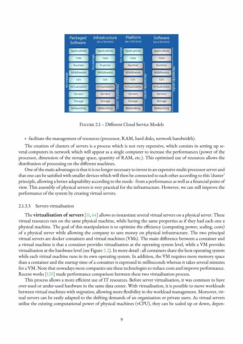
Figure 2.1 – Different Cloud Service Models

∗ facilitate the management of resources (processor, RAM, hard disks, network bandwidth).The creation of clusters of servers is a process which is not very expensive, which consists in setting up se-

veral computers in network which will appear as a single computer to increase the performances (power of theprocessor, dimension of the storage space, quantity of RAM, etc.). This optimised use of resources allows thedistribution of processing on the different machines.

One of themain advantages is that it is no longer necessary to invest in an expensivemulti-processor server andthat one can be satisfied with smaller devices which will then be connected to each other according to this ’cluster’principle, allowing a better adaptability according to the needs - from a performance as well as a financial point ofview. This assembly of physical servers is very practical for the infrastructure. However, we can still improve theperformance of the system by creating virtual servers.

2.1.3.3 Servers virtualisation

The virtualisation of servers [11, 64] allows to instantiate several virtual servers on a physical server. Thesevirtual resources run on the same physical machine, while having the same properties as if they had each one aphysical machine. The goal of this manipulation is to optimise the efficiency (computing power, scaling, costs)of a physical server while allowing the company to save money on physical infrastructure. The two principalvirtual servers are docker containers and virtual machines (VMs). The main difference between a container anda virtual machine is that a container provides virtualisation at the operating system level, while a VM providesvirtualisation at the hardware level (see Figure 2.2). In more detail : all containers share the host operating systemwhile each virtual machine runs in its own operating system. In addition, the VM requires more memory spacethan a container and the startup time of a container is expressed in milliseconds whereas it takes several minutesfor a VM.Note that nowadays most companies use these technologies to reduce costs and improve performance.Recent works [120] made performance comparison between these two virtualisation process.

This process allows a more efficient use of IT resources. Before server virtualisation, it was common to haveover-used or under-used hardware in the same data center. With virtualisation, it is possible to move workloadsbetween virtual machines withmigration, allowing more flexibility in the workload management. Moreover, vir-tual servers can be easily adapted to the shifting demands of an organisation or private users. As virtual serversutilise the existing computational power of physical machines (vCPU), they can be scaled up or down, depen-

9

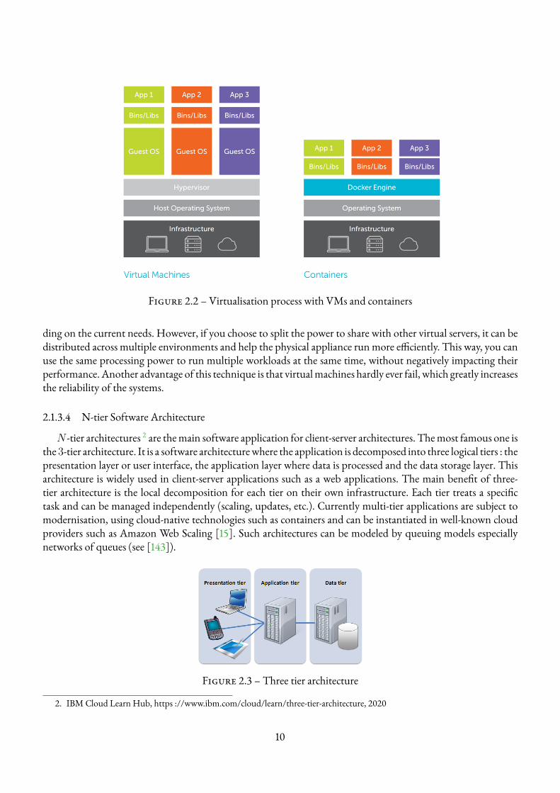
Figure 2.2 – Virtualisation process with VMs and containers

ding on the current needs. However, if you choose to split the power to share with other virtual servers, it can bedistributed across multiple environments and help the physical appliance runmore efficiently. This way, you canuse the same processing power to run multiple workloads at the same time, without negatively impacting theirperformance. Another advantage of this technique is that virtualmachines hardly ever fail, which greatly increasesthe reliability of the systems.

2.1.3.4 N-tier Software Architecture

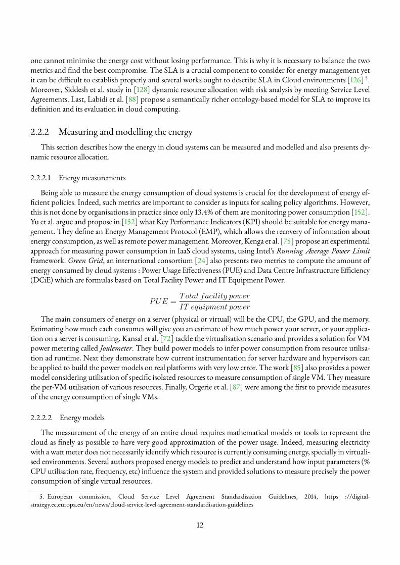
N -tier architectures 2 are themain software application for client-server architectures. Themost famous one isthe3-tier architecture. It is a software architecturewhere the application is decomposed into three logical tiers : thepresentation layer or user interface, the application layer where data is processed and the data storage layer. Thisarchitecture is widely used in client-server applications such as a web applications. The main benefit of three-tier architecture is the local decomposition for each tier on their own infrastructure. Each tier treats a specifictask and can be managed independently (scaling, updates, etc.). Currently multi-tier applications are subject tomodernisation, using cloud-native technologies such as containers and can be instantiated in well-known cloudproviders such as Amazon Web Scaling [15]. Such architectures can be modeled by queuing models especiallynetworks of queues (see [143]).

Figure 2.3 – Three tier architecture

2. IBM Cloud Learn Hub, https ://www.ibm.com/cloud/learn/three-tier-architecture, 2020

10

2.2 Energy management

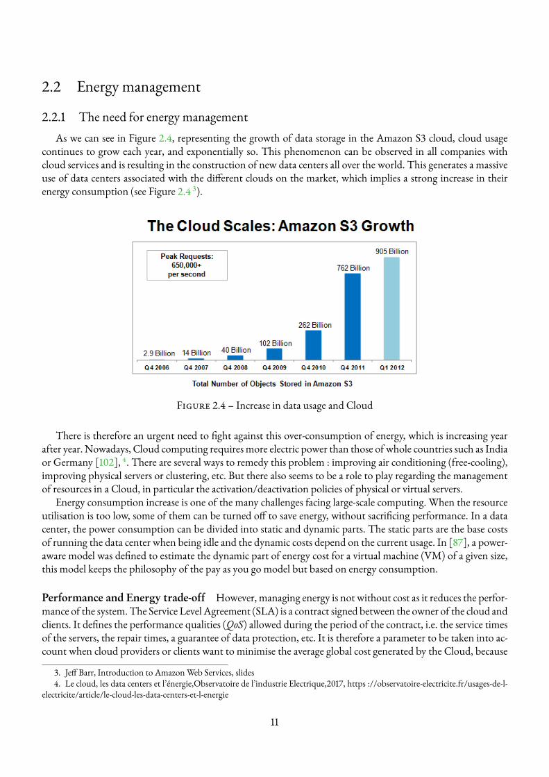
2.2.1 The need for energy managementAs we can see in Figure 2.4, representing the growth of data storage in the Amazon S3 cloud, cloud usage

continues to grow each year, and exponentially so. This phenomenon can be observed in all companies withcloud services and is resulting in the construction of new data centers all over the world. This generates a massiveuse of data centers associated with the different clouds on the market, which implies a strong increase in theirenergy consumption (see Figure 2.4 3).

Figure 2.4 – Increase in data usage and Cloud

There is therefore an urgent need to fight against this over-consumption of energy, which is increasing yearafter year. Nowadays, Cloud computing requires more electric power than those of whole countries such as Indiaor Germany [102], 4. There are several ways to remedy this problem : improving air conditioning (free-cooling),improving physical servers or clustering, etc. But there also seems to be a role to play regarding the managementof resources in a Cloud, in particular the activation/deactivation policies of physical or virtual servers.

Energy consumption increase is one of the many challenges facing large-scale computing. When the resourceutilisation is too low, some of them can be turned off to save energy, without sacrificing performance. In a datacenter, the power consumption can be divided into static and dynamic parts. The static parts are the base costsof running the data center when being idle and the dynamic costs depend on the current usage. In [87], a power-aware model was defined to estimate the dynamic part of energy cost for a virtual machine (VM) of a given size,this model keeps the philosophy of the pay as you go model but based on energy consumption.

Performance and Energy trade-off However, managing energy is not without cost as it reduces the perfor-mance of the system. The Service Level Agreement (SLA) is a contract signed between the owner of the cloud andclients. It defines the performance qualities (QoS) allowed during the period of the contract, i.e. the service timesof the servers, the repair times, a guarantee of data protection, etc. It is therefore a parameter to be taken into ac-count when cloud providers or clients want to minimise the average global cost generated by the Cloud, because

3. Jeff Barr, Introduction to AmazonWeb Services, slides4. Le cloud, les data centers et l’énergie,Observatoire de l’industrie Electrique,2017, https ://observatoire-electricite.fr/usages-de-l-

electricite/article/le-cloud-les-data-centers-et-l-energie

11

one cannot minimise the energy cost without losing performance. This is why it is necessary to balance the twometrics and find the best compromise. The SLA is a crucial component to consider for energy management yetit can be difficult to establish properly and several works ought to describe SLA in Cloud environments [126] 5.Moreover, Siddesh et al. study in [128] dynamic resource allocation with risk analysis by meeting Service LevelAgreements. Last, Labidi et al. [88] propose a semantically richer ontology-based model for SLA to improve itsdefinition and its evaluation in cloud computing.

2.2.2 Measuring and modelling the energyThis section describes how the energy in cloud systems can be measured and modelled and also presents dy-

namic resource allocation.

2.2.2.1 Energy measurements

Being able to measure the energy consumption of cloud systems is crucial for the development of energy ef-ficient policies. Indeed, such metrics are important to consider as inputs for scaling policy algorithms. However,this is not done by organisations in practice since only 13.4% of them are monitoring power consumption [152].Yu et al. argue and propose in [152] what Key Performance Indicators (KPI) should be suitable for energy mana-gement. They define an Energy Management Protocol (EMP), which allows the recovery of information aboutenergy consumption, as well as remote powermanagement.Moreover, Kenga et al. [75] propose an experimentalapproach for measuring power consumption in IaaS cloud systems, using Intel’s Running Average Power Limitframework. Green Grid, an international consortium [24] also presents two metrics to compute the amount ofenergy consumed by cloud systems : Power Usage Effectiveness (PUE) and Data Centre Infrastructure Efficiency(DCiE) which are formulas based on Total Facility Power and IT Equipment Power.

PUE =Total facility power

IT equipment power

The main consumers of energy on a server (physical or virtual) will be the CPU, the GPU, and the memory.Estimating howmuch each consumes will give you an estimate of howmuch power your server, or your applica-tion on a server is consuming. Kansal et al. [72] tackle the virtualisation scenario and provides a solution for VMpower metering called Joulemeter. They build power models to infer power consumption from resource utilisa-tion ad runtime. Next they demonstrate how current instrumentation for server hardware and hypervisors canbe applied to build the power models on real platforms with very low error. The work [85] also provides a powermodel considering utilisation of specific isolated resources to measure consumption of single VM. Theymeasurethe per-VM utilisation of various resources. Finally, Orgerie et al. [87] were among the first to provide measuresof the energy consumption of single VMs.

2.2.2.2 Energy models

The measurement of the energy of an entire cloud requires mathematical models or tools to represent thecloud as finely as possible to have very good approximation of the power usage. Indeed, measuring electricitywith a wattmeter does not necessarily identify which resource is currently consuming energy, specially in virtuali-sed environments. Several authors proposed energy models to predict and understand how input parameters (%CPU utilisation rate, frequency, etc) influence the system and provided solutions to measure precisely the powerconsumption of single virtual resources.

5. European commission, Cloud Service Level Agreement Standardisation Guidelines, 2014, https ://digital-strategy.ec.europa.eu/en/news/cloud-service-level-agreement-standardisation-guidelines

12

In data centers or cloud environments, the server power consumption can be divided into static and dynamicparts. The static part (which does not vary with workload) represents the energy consumed by a server when itis idle, while the dynamic cost depends on the current usage. Orgerie et al. [87] define a power-aware model toestimate the dynamic part of energy cost for a VM of a given size, this model keeps the philosophy of the pay asyou go model but it is based on energy consumption.

In addition, Benoit et al. [25] review and derive several models under different assumptions (idle, turningon/off costs, time, energy, etc.). Considering On/Off policies is well-known in the literature but can be highlydifferent if one consider that there exists execution time or energy costs to activate or deactivate resources. Theyshow sequence awaremodels that can be based on time or energy constraints. In each model is respectively inte-grated the turn-off time of VM and the energy cost for switching off. Finally, Zhou et al. [155] also presents afine-grained energy consumption model and analyses its efficiency in energy consumption of data centers. Theirgoal is to reduce energy consumption while meeting the quality of service.

With energy measurements and models, cloud providers or customers have the necessary metrics and modelsto take as inputs for energy-efficient policies. The following treats about how to manage the energy and findefficient scaling policies in cloud environments.

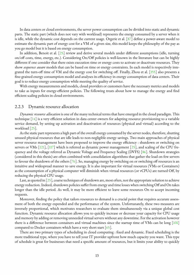
2.2.3 Dynamic resource allocationDynamic resource allocation is one of themany technical terms that have emerged in the cloud paradigm. This

technique [14] is a very efficient solution in data center owners for adapting resource provisioning to a variableservice demand, by setting up activation and deactivation of resources (physical and virtual) according to theworkload [25].

As the static part represents a high part of the overall energy consumed by the server nodes, therefore, shuttingunused physical resources that are idle leads to non-negligible energy savings. Two main approaches of physicalserver resource management have been proposed to improve the energy efficiency : shutdown or switching onservers or VMs [121], [117] which is referred as dynamic power management [25], and scaling of the CPU fre-quency and the voltage referred as Dynamic Voltage and Frequency Scaling (DVFS) [86]. Shutdown strategies(considered in this thesis) are often combined with consolidation algorithms that gather the load on few serversto favour the shutdown of the others [76]. So, managing energy by switching on or switching off resources is anintuitive and widespread manner to save energy. It is also important for virtual resources (VMs or Containers)as the consumption of a physical computer will diminish when virtual resources (or vCPUs) are turned Off, byreducing the physical CPU usage.

Last, as quoted in [25], coarse techniques of shutdown are,most often, not the appropriate solution to achieveenergy reduction. Indeed, shutdown policies suffer from energy and time losses when switchingOff andOn takeslonger than the idle period. As well, it may be more efficient to leave some resources On to accept incomingrequests.

Moreover, finding the policy that tailors resources to demand is a crucial point that requires accurate assess-ment of both the energy expended and the performance of the system. Unfortunately, these two measures areinversely proportional, which motivates researchers to evaluate them simultaneously via a unique global costfunction. Dynamic resource allocation allows you to quickly increase or decrease your capacity for CPU usageandmemory by adding or removing unneeded virtual servers without any downtime. For the activation howeverthere is a difference between containers and virtual machines since the startup time of VMs can be long [101]compared to Docker containers which have a very short start [65].

There are two primary types of scheduling in cloud computing : fixed and dynamic. Fixed scheduling is themore traditional type, where you have to tell your IT provider upfront how much capacity you want. This typeof schedule is great for businesses that need a specific amount of resources, but it limits your ability to quickly

13

grow or decrease your need. Dynamic scheduling, on the other hand, allows businesses to adjust their capacityas needed without any downtime. This is ideal for those who may not know exactly how much capacity they’llneed at certain points in time or those who want an easier way to scale up and down as needed (e.g., e-commercecompanies). The adjustment of capacity can be done with specific rules such as auto-scaling policies.

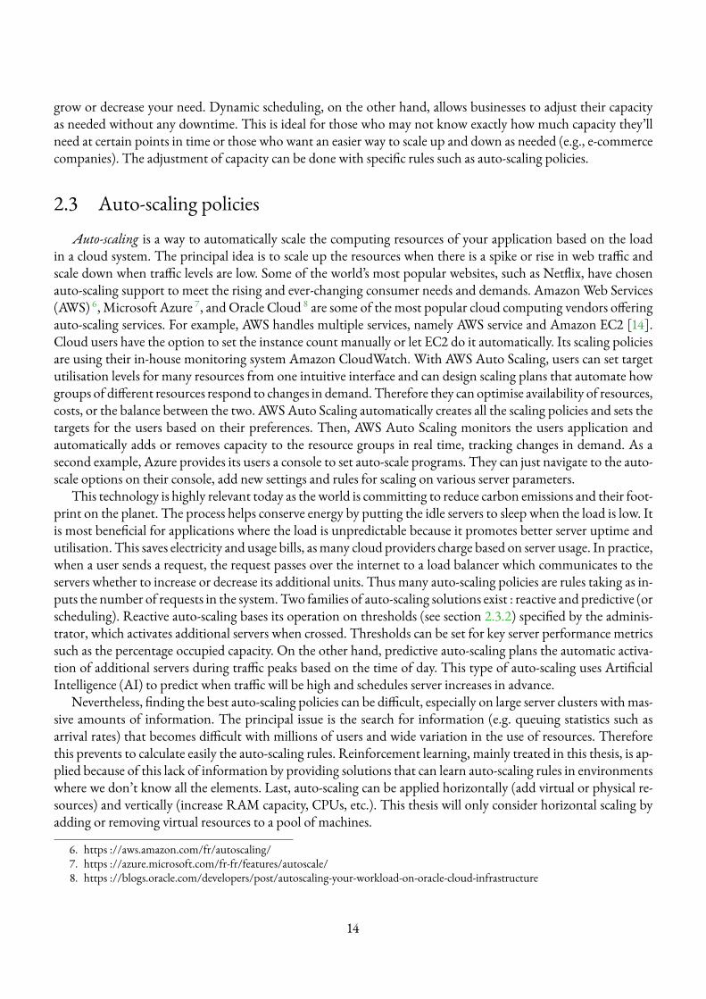
2.3 Auto-scaling policiesAuto-scaling is a way to automatically scale the computing resources of your application based on the load

in a cloud system. The principal idea is to scale up the resources when there is a spike or rise in web traffic andscale down when traffic levels are low. Some of the world’s most popular websites, such as Netflix, have chosenauto-scaling support to meet the rising and ever-changing consumer needs and demands. Amazon Web Services(AWS) 6, Microsoft Azure 7, and Oracle Cloud 8 are some of the most popular cloud computing vendors offeringauto-scaling services. For example, AWS handles multiple services, namely AWS service and Amazon EC2 [14].Cloud users have the option to set the instance count manually or let EC2 do it automatically. Its scaling policiesare using their in-house monitoring system Amazon CloudWatch. With AWS Auto Scaling, users can set targetutilisation levels for many resources from one intuitive interface and can design scaling plans that automate howgroups of different resources respond to changes in demand.Therefore they can optimise availability of resources,costs, or the balance between the two. AWSAuto Scaling automatically creates all the scaling policies and sets thetargets for the users based on their preferences. Then, AWS Auto Scaling monitors the users application andautomatically adds or removes capacity to the resource groups in real time, tracking changes in demand. As asecond example, Azure provides its users a console to set auto-scale programs. They can just navigate to the auto-scale options on their console, add new settings and rules for scaling on various server parameters.

This technology is highly relevant today as the world is committing to reduce carbon emissions and their foot-print on the planet. The process helps conserve energy by putting the idle servers to sleep when the load is low. Itis most beneficial for applications where the load is unpredictable because it promotes better server uptime andutilisation. This saves electricity and usage bills, asmany cloud providers charge based on server usage. In practice,when a user sends a request, the request passes over the internet to a load balancer which communicates to theservers whether to increase or decrease its additional units. Thus many auto-scaling policies are rules taking as in-puts the number of requests in the system.Two families of auto-scaling solutions exist : reactive and predictive (orscheduling). Reactive auto-scaling bases its operation on thresholds (see section 2.3.2) specified by the adminis-trator, which activates additional servers when crossed. Thresholds can be set for key server performance metricssuch as the percentage occupied capacity. On the other hand, predictive auto-scaling plans the automatic activa-tion of additional servers during traffic peaks based on the time of day. This type of auto-scaling uses ArtificialIntelligence (AI) to predict when traffic will be high and schedules server increases in advance.

Nevertheless, finding the best auto-scaling policies can be difficult, especially on large server clusters withmas-sive amounts of information. The principal issue is the search for information (e.g. queuing statistics such asarrival rates) that becomes difficult with millions of users and wide variation in the use of resources. Thereforethis prevents to calculate easily the auto-scaling rules. Reinforcement learning, mainly treated in this thesis, is ap-plied because of this lack of information by providing solutions that can learn auto-scaling rules in environmentswhere we don’t know all the elements. Last, auto-scaling can be applied horizontally (add virtual or physical re-sources) and vertically (increase RAM capacity, CPUs, etc.). This thesis will only consider horizontal scaling byadding or removing virtual resources to a pool of machines.

6. https ://aws.amazon.com/fr/autoscaling/7. https ://azure.microsoft.com/fr-fr/features/autoscale/8. https ://blogs.oracle.com/developers/post/autoscaling-your-workload-on-oracle-cloud-infrastructure

14

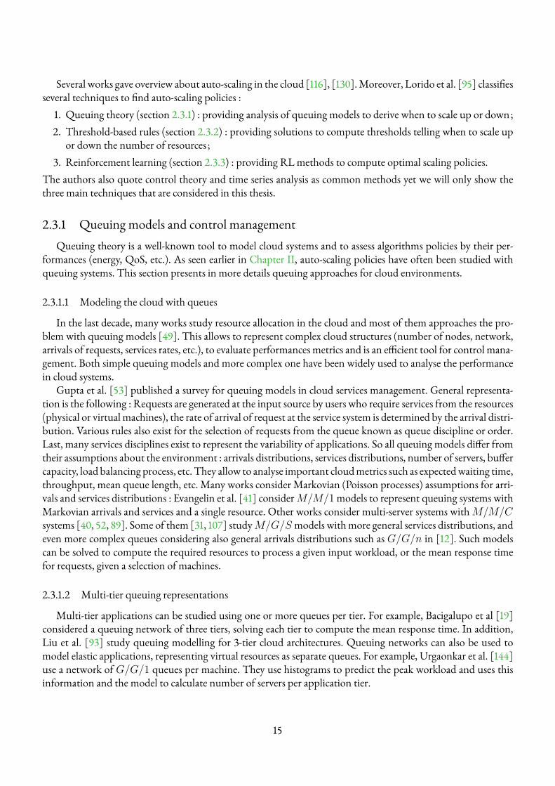
Several works gave overview about auto-scaling in the cloud [116], [130].Moreover, Lorido et al. [95] classifiesseveral techniques to find auto-scaling policies :

1. Queuing theory (section 2.3.1) : providing analysis of queuing models to derive when to scale up or down;2. Threshold-based rules (section 2.3.2) : providing solutions to compute thresholds telling when to scale up

or down the number of resources ;3. Reinforcement learning (section 2.3.3) : providing RLmethods to compute optimal scaling policies.

The authors also quote control theory and time series analysis as common methods yet we will only show thethree main techniques that are considered in this thesis.

2.3.1 Queuing models and control managementQueuing theory is a well-known tool to model cloud systems and to assess algorithms policies by their per-

formances (energy, QoS, etc.). As seen earlier in Chapter II, auto-scaling policies have often been studied withqueuing systems. This section presents in more details queuing approaches for cloud environments.

2.3.1.1 Modeling the cloud with queues

In the last decade, many works study resource allocation in the cloud and most of them approaches the pro-blem with queuing models [49]. This allows to represent complex cloud structures (number of nodes, network,arrivals of requests, services rates, etc.), to evaluate performances metrics and is an efficient tool for control mana-gement. Both simple queuing models and more complex one have been widely used to analyse the performancein cloud systems.

Gupta et al. [53] published a survey for queuing models in cloud services management. General representa-tion is the following : Requests are generated at the input source by users who require services from the resources(physical or virtual machines), the rate of arrival of request at the service system is determined by the arrival distri-bution. Various rules also exist for the selection of requests from the queue known as queue discipline or order.Last, many services disciplines exist to represent the variability of applications. So all queuing models differ fromtheir assumptions about the environment : arrivals distributions, services distributions, number of servers, buffercapacity, load balancing process, etc. They allow to analyse important cloudmetrics such as expectedwaiting time,throughput, mean queue length, etc. Many works consider Markovian (Poisson processes) assumptions for arri-vals and services distributions : Evangelin et al. [41] considerM/M/1models to represent queuing systems withMarkovian arrivals and services and a single resource. Other works consider multi-server systems withM/M/Csystems [40, 52, 89]. Some of them [31, 107] studyM/G/Smodels withmore general services distributions, andeven more complex queues considering also general arrivals distributions such as G/G/n in [12]. Such modelscan be solved to compute the required resources to process a given input workload, or the mean response timefor requests, given a selection of machines.

2.3.1.2 Multi-tier queuing representations

Multi-tier applications can be studied using one or more queues per tier. For example, Bacigalupo et al [19]considered a queuing network of three tiers, solving each tier to compute the mean response time. In addition,Liu et al. [93] study queuing modelling for 3-tier cloud architectures. Queuing networks can also be used tomodel elastic applications, representing virtual resources as separate queues. For example, Urgaonkar et al. [144]use a network of G/G/1 queues per machine. They use histograms to predict the peak workload and uses thisinformation and the model to calculate number of servers per application tier.

15

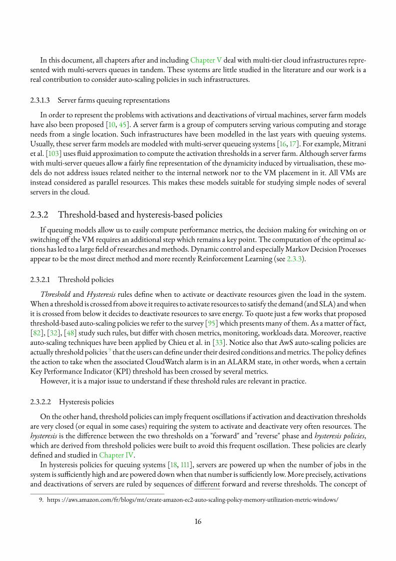
In this document, all chapters after and including Chapter V deal with multi-tier cloud infrastructures repre-sented with multi-servers queues in tandem. These systems are little studied in the literature and our work is areal contribution to consider auto-scaling policies in such infrastructures.

2.3.1.3 Server farms queuing representations

In order to represent the problems with activations and deactivations of virtual machines, server farmmodelshave also been proposed [10, 45]. A server farm is a group of computers serving various computing and storageneeds from a single location. Such infrastructures have been modelled in the last years with queuing systems.Usually, these server farmmodels are modeled with multi-server queueing systems [16, 17]. For example, Mitraniet al. [103] uses fluid approximation to compute the activation thresholds in a server farm. Although server farmswith multi-server queues allow a fairly fine representation of the dynamicity induced by virtualisation, these mo-dels do not address issues related neither to the internal network nor to the VM placement in it. All VMs areinstead considered as parallel resources. This makes these models suitable for studying simple nodes of severalservers in the cloud.

2.3.2 Threshold-based and hysteresis-based policiesIf queuing models allow us to easily compute performance metrics, the decision making for switching on or

switching off the VM requires an additional step which remains a key point. The computation of the optimal ac-tions has led to a large field of researches andmethods.Dynamic control and especiallyMarkovDecisionProcessesappear to be the most direct method and more recently Reinforcement Learning (see 2.3.3).

2.3.2.1 Threshold policies

Threshold and Hysteresis rules define when to activate or deactivate resources given the load in the system.When a threshold is crossed fromabove it requires to activate resources to satisfy the demand (and SLA) andwhenit is crossed from below it decides to deactivate resources to save energy. To quote just a few works that proposedthreshold-based auto-scaling policies we refer to the survey [95]which presentsmany of them.As amatter of fact,[82], [32], [48] study such rules, but differ with chosen metrics, monitoring, workloads data. Moreover, reactiveauto-scaling techniques have been applied by Chieu et al. in [33]. Notice also that AwS auto-scaling policies areactually thresholdpolicies 9 that theusers candefineunder their desired conditions andmetrics.Thepolicy definesthe action to take when the associated CloudWatch alarm is in an ALARM state, in other words, when a certainKey Performance Indicator (KPI) threshold has been crossed by several metrics.

However, it is a major issue to understand if these threshold rules are relevant in practice.

2.3.2.2 Hysteresis policies

On the other hand, threshold policies can imply frequent oscillations if activation and deactivation thresholdsare very closed (or equal in some cases) requiring the system to activate and deactivate very often resources. Thehysteresis is the difference between the two thresholds on a "forward" and "reverse" phase and hysteresis policies,which are derived from threshold policies were built to avoid this frequent oscillation. These policies are clearlydefined and studied in Chapter IV.

In hysteresis policies for queuing systems [18, 111], servers are powered up when the number of jobs in thesystem is sufficiently high and are powered downwhen that number is sufficiently low.More precisely, activationsand deactivations of servers are ruled by sequences of different forward and reverse thresholds. The concept of

9. https ://aws.amazon.com/fr/blogs/mt/create-amazon-ec2-auto-scaling-policy-memory-utilization-metric-windows/

16

hysteresis can also be applied to the control of service rates. They allow not to activate and deactivate the serverstoo frequently when the load is varying. This makes it possible to correctly adapt variable resources accordingto demand by means of thresholds [78, 98]. Therefore, multi-server queueing systems working with thresholds-based policies and verifying hysteresis properties have been suggested to efficiently manage the number of activeVMs [127, 141]. More recently, Dutreilh et al. [39] stated that thresholds need to be carefully tuned to avoidfrequent oscillations in the system, thus considering hysteresis properties.

The other advantage that makes hysteresis policies so appealing is their ease of implementation. This is why,they are a key component of the auto-scaling systems for thewidespread cloud architecturesKubernetes for dockercomponents, andAzure orAmazonWeb Services [14] for virtualmachines.Henceforth, there is a great interest ofstudying the computation of hysteresis policy since threshold values can be plugged into auto-scaling systems thatare implemented in the major cloud architectures. Researches on hysteresis policies are twofold : first explorationof the conditions that insure the optimality of hysteresis policy. The second axis studies the computation of thethreshold values.

2.3.2.3 Optimality of threshold and hysteresis rules

It exists in the literature several works studying the structure of the optimal policy in queuing systems [62, 81],network and finally Cloud. Federgruen et al. [42] show optimality of threshold policies in single-server queuingsystems with server vacations. Yang et al. [150] also study structural properties of the optimal resource allocationpolicy for single-queue systems. The optimal number of servers follows a step function following a bang-bangcontrol policy. Yang et al. provide conditions under which the bang-bang control policy takes place. In optimalcontrol problems, it often happens that a control is bounded by a lower and an upper bound. If the optimalcontrol goes from one extreme to the other (i.e., it is strictly never between the two bounds), it is called a bang-bang control policy. Also in [94] is shown that under some assumptions the optimal policy in a tandem queuesystem is a bang-bang control policy with monotonicity properties.

For hysteresis rules, it appeared very early in the work of Bell for aM/M/2 queuing model [137], that theoptimal policy in suchmodels has a special formand is calledhysteresis. In addition, Szarkowicz et al. [134] showedthe optimality of hysteresis policies in aM/M/S queuing model with a control of the vacations of the servers.For models with control of the service rates, the proofs were made inHipp [58] in the 80s and in Serfozo [78] forM/M/1 queues in the 90s.

2.3.2.4 Computation of threshold and hysteresis rules

Now, creating the rules requires an effort from the clients (or cloud providers), who need to select the suitableperformancemetrics andneed to define carefully thresholds.Moreover it is stated in [95] that it is difficult to selectthe corresponding thresholds in real systems. Indeed, the calculation of effective threshold values first encounterthe same difficulties as single threshold policies (base-stock policies).

For hysteresis models, the calculation of optimal thresholds received few attention in the past and two ma-jor trends appeared. The computation of the optimal policy can be done by means of adapted usual dynamicprogramming algorithms in which the structured policies properties are plugged. A similar treatment has beenaddressed for routing in [110]. The alternate way is similar to the single threshold research for base-stock policieswhich is very common in inventory management. A local search in the works [84, 118] is used to explore the op-timal thresholds. The computation of expected measures associated with a set of thresholds is complex [28]. Itrequires the computation of the stationary distribution either by standard numerical methods see e.g. [149] orafter a Markovian analysis with simpler and faster computations (e.g. [146] uses iterative methods to computethe stationary distribution). As cloud systems are modelled by multi-dimensional systems, defined on very largestate spaces, then the stationary distribution computation is difficult. Fortunately, the computation of the per-

17

formancemeasures of hysteresis multi-server systems has been already studied in the literature. Different efficientresolutionmethods have been developed. Among themost significant works, we quote the work of Ibe and Keil-son [63] refined in Lui and Golubchik [98]. Both solve the model by partitioning the state space in disjoint setsto aggregate theMarkov chain. Exhaustive comparisons of the resolutionmethods are made in [71] : closed-formsolution of the stationary distribution, partition of the state space, and matrix geometric methods applied onQBD (Quasi birth and death) processes are studied.

In [6], Song et al. claims that, for single threshold models, the second approach dealing with stationary distri-bution computations are generally more effective thanMarkov Decision Process approaches. Such a comparisonhas not been performed yet for hysteresis especially since few works implement aMDP algorithmwith a structu-red policy. Chapter IV proposes and compares twomathematical approaches to compute optimal thresholds andhysteresis policies under specific assumptions (also see [139]).

2.3.3 Reinforcement Learning for cloud resource allocationNumerous works have been devoted to compute optimal policy inmulti-server queuemodels withMDP (see

[139] and references therein). However, Markov Decision Process framework requires a perfect knowledge ofthe model (queuing statistics such as arrival or service distributions etc.). Unhappily, these values are not alwaysknown in practice and Reinforcement Learning techniques should be applied to dynamic resource allocation toovercome this lack of information. Without any a priori knowledge, RL methods can determine the best sca-ling decision to take in each state, given the input workload. This section first displays MDP approaches whereknowledge of the environment is given to the agent, then auto-scaling RL solutions [46] where environmentsinformation are unknown (statistics, users, etc.).

2.3.3.1 Markov Decision Process approaches

Markov Decision Process has been widely used to model resource management problems including auto-scaling problems. Different algorithms exist to find the optimal management policy, when the underlying transi-tionprobabilities are known [139]. Since the seminalwork ofMcGill in 1969 (with anoptimal controlmodel) andthat of Lippman (with a Markov decision process model) numerous works have been devoted to similar multi-server queue models using Markov decision processes (see [137] and references therein for the oldest, and morerecently [151] and [90] to quote just a few). Moreover, [91] is a recent survey aboutMDP approaches for queuesand networks. It reviews all MDP applications for control in queuing and networking systems. For example,Okamura et al. [112] study MDP approaches for dynamic power management problems in order to save powerconsumption. They consider an optimal power-aware design in a cloud system represented by a cluster. Unfor-tunately, not all of them received rigorous treatment and the study of unichain or multichain property is oftenignored.

Now, these works require full knowledge of the environment which is not obvious in real cloud systems. Toovercome this issue and deal with missing information about environments, reinforcement learning methodshave been applied.

2.3.3.2 Reinforcement learning approaches

Again, two surveys [46, 95] address reinforcement learning for auto-scaling policies in cloud environments.Many works for RL application on cloud resource allocation problems are discussed and different taxonomiesabout the resolution techniques, the criteria to optimise as well as the type of problem are presented. As men-tioned earlier, RL techniques can learn the optimal auto-scaling policy without requiring the knowledge of thestatistics of the system : either it learns from experience in a model-free fashion or the agent aims to learn this

18

knowledge in a model-based fashion. Following [46], we decompose this paragraph in two parts : model-free RLapplications and model-based applications.

Model-free techniques : Most of the RL techniques applied to resource allocation in the cloud aremodel-freeand the vastmajority of themare standardQ-learning andDeepQ-learning techniques. For example, amodel-freereinforcement learning technique withQ-Learning for autonomic resource allocation in the cloud was proposedbyDutreilh et al. in [38]. In thiswork an agent has to control the number of resources andoptimise a cost functionthat takes into account virtualmachines costs andSLA.They focus on a single physical nodehosting several virtualresources and consider the (w;u; p) state definition, where p stands for performance in terms of average responsetime to requests,w for workload and u the number of virtual servers. An other example is the work fromTesauroet al. [138]. They propose model-free RL using (w;ut−1;ut) state representation, where w is the total numberof user requests observed per time period; ut and ut−1 are the number of activated VMs in the current time step,and the previous time step, respectively. This representationwill be used along the thesis (i.e. considering numberof requests and VMs at each time step).

For our problem, Jin et al. [68] propose Q-learning to derive auto-scaling policies in the cloud to minimisedelays and number of activated resources and consider again a single physical node. To quotemore, the followingworks focus mainly onQ-learning algorithm on a single physical node but have different optimisation criteria orstate space : the work [61] considers the response time and the average resource utilization and [148] proposesan approach based on inhomogeneous VM.More recently and inmodern networks, works have been presentingRL solutions [77] for 5G network slicing and [80, 124] for slicing with Deep RL, to quote just a few.

However, many works raise performance issues with model-free RL techniques. Indeed, the problem of poorperformances in the early steps has been addressed in a number ofways. The principal problem is the lack of initialinformation and the randomness of the exploration policy. For this reason,Dutreilh et al. [39] proposed a customheuristic to guide the state space exploration. They also propose an initial approximation of the Q-function thatupdates the value for all states at each iteration, and also speeds up the convergence to the optimal policy. Otherworks have also attempted to reduce this training time. It is addressedwith an exploration policy that visits severalstates at each step [119] or using parallel learning agents [22]. In the latter, learning agents do not need to visitevery state and action since they can learn the value of non-visited states from neighboring agents.

Overall, many works show that while model-free RL techniques hold great promise for learning adaptivecontrol policies, it still suffers from slow convergence and detrimental randomexploration. So this appeal to studynew paradigm of RL techniques to overcome these issues.

Model-based techniques : Although researchers have attempted to improvemodel-free techniques, very fewofthem have tried to apply model-based RL approaches. In this context, model-based reinforcement learning tech-niques [106] can decrease exploration steps by learning amodel of the environment, allowing the agent to updatefaster theQ-Value by a supplementary planning phase. Nevertheless, [46]mentions only twoworks that are clas-sified as usingmodel-based techniques forCloud auto-scaling scenarios and these twoworks ought to estimate thetransition probabilities and thereafter solve the problem with MDP algorithms. Hence, due to the requirementof having a complete model of the environment in model-based methods, [21] estimates the probability distri-bution of the transition between states by counting occurrences of visits in state-action pairs (s, a) and (s, a, s′)and the planning of the policy is done in an offlinemode, by comparingMDP resolution algorithmswithGeneticAlgorithm. However, as quoted in [106], the model based framework is larger than the simple models presentedin [46]. This, coupledwith the very few amount of works in literature aboutmodel-based reinforcement learningfor cloud applications call for further research in this topic and for comparison of model-free algorithms.

Therefore, there is a great interest to study model-based techniques and compared them with state of the artmodel-free RL methods. This is the main application in Chapter V. On the other hand, it could be extremelyvaluable to devise methods that limit the dimensionality while offering more guarantees of accuracy and greaterexplainability. This is the goal of the last two chapters which improves model-based RLmethods by considering

19

state variables dependencies as a knowledge for the agent. Hence, Chapter VI deals with factored representationand Chapter VII deals with causal representation.

20

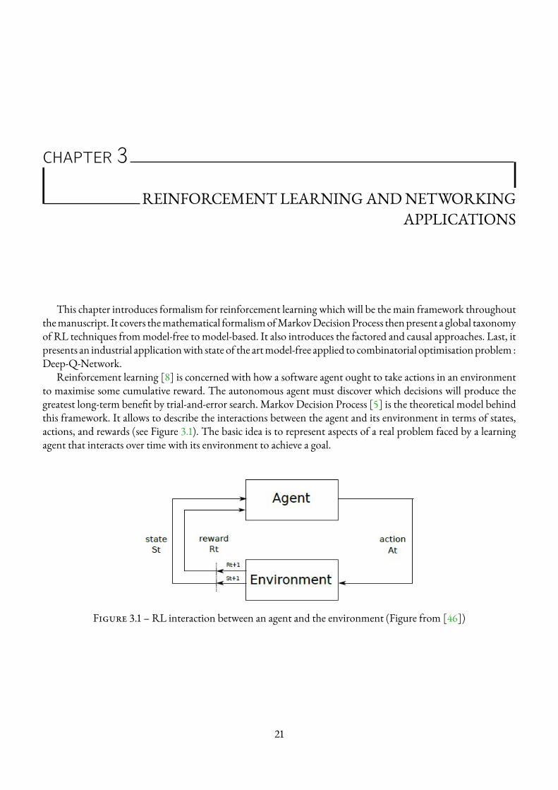
CHAPTER 3

REINFORCEMENT LEARNINGANDNETWORKINGAPPLICATIONS

This chapter introduces formalism for reinforcement learning which will be the main framework throughoutthemanuscript. It covers themathematical formalismofMarkovDecisionProcess thenpresent a global taxonomyof RL techniques frommodel-free to model-based. It also introduces the factored and causal approaches. Last, itpresents an industrial applicationwith state of the artmodel-free applied to combinatorial optimisationproblem :Deep-Q-Network.

Reinforcement learning [8] is concerned with how a software agent ought to take actions in an environmentto maximise some cumulative reward. The autonomous agent must discover which decisions will produce thegreatest long-term benefit by trial-and-error search. Markov Decision Process [5] is the theoretical model behindthis framework. It allows to describe the interactions between the agent and its environment in terms of states,actions, and rewards (see Figure 3.1). The basic idea is to represent aspects of a real problem faced by a learningagent that interacts over time with its environment to achieve a goal.

Figure 3.1 – RL interaction between an agent and the environment (Figure from [46])

21

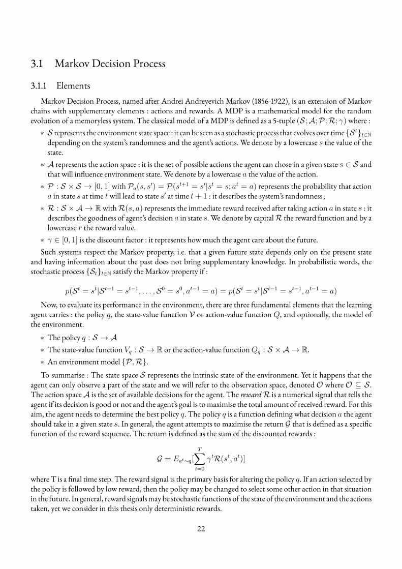
3.1 Markov Decision Process

3.1.1 ElementsMarkov Decision Process, named after Andrei Andreyevich Markov (1856-1922), is an extension of Markov

chains with supplementary elements : actions and rewards. A MDP is a mathematical model for the randomevolution of a memoryless system. The classical model of a MDP is defined as a 5-tuple (S;A;P ;R; γ) where :∗ S represents the environment state space : it canbe seen as a stochastic process that evolves over time{St}t∈Ndepending on the system’s randomness and the agent’s actions. We denote by a lowercase s the value of thestate.∗ A represents the action space : it is the set of possible actions the agent can chose in a given state s ∈ S andthat will influence environment state. We denote by a lowercase a the value of the action.∗ P : S × S → [0, 1] withPa(s, s′) = P(st+1 = s′|st = s; at = a) represents the probability that actiona in state s at time twill lead to state s′ at time t+ 1 : it describes the system’s randomness ;∗ R : S ×A → RwithR(s, a) represents the immediate reward received after taking action a in state s : itdescribes the goodness of agent’s decision a in state s. We denote by capitalR the reward function and by alowercase r the reward value.∗ γ ∈ [0, 1] is the discount factor : it represents howmuch the agent care about the future.Such systems respect the Markov property, i.e. that a given future state depends only on the present state

and having information about the past does not bring supplementary knowledge. In probabilistic words, thestochastic process {St}t∈N satisfy the Markov property if :

p(St = st|St−1 = st−1, . . . ,S0 = s0, at−1 = a) = p(St = st|St−1 = st−1, at−1 = a)

Now, to evaluate its performance in the environment, there are three fundamental elements that the learningagent carries : the policy q, the state-value function V or action-value function Q, and optionally, the model ofthe environment.

∗ The policy q : S → A∗ The state-value function Vq : S → R or the action-value functionQq : S ×A → R.∗ An environment model {P ,R}.To summarise : The state space S represents the intrinsic state of the environment. Yet it happens that the

agent can only observe a part of the state and we will refer to the observation space, denotedO whereO ⊆ S .The action spaceA is the set of available decisions for the agent. The rewardR is a numerical signal that tells theagent if its decision is good or not and the agent’s goal is tomaximise the total amount of received reward. For thisaim, the agent needs to determine the best policy q. The policy q is a function defining what decision a the agentshould take in a given state s. In general, the agent attempts to maximise the return G that is defined as a specificfunction of the reward sequence. The return is defined as the sum of the discounted rewards :

G = Eat∼q[T∑t=0

γtR(st, at)]

where T is a final time step. The reward signal is the primary basis for altering the policy q. If an action selected bythe policy is followed by low reward, then the policy may be changed to select some other action in that situationin the future. In general, reward signalsmaybe stochastic functions of the state of the environment and the actionstaken, yet we consider in this thesis only deterministic rewards.

22

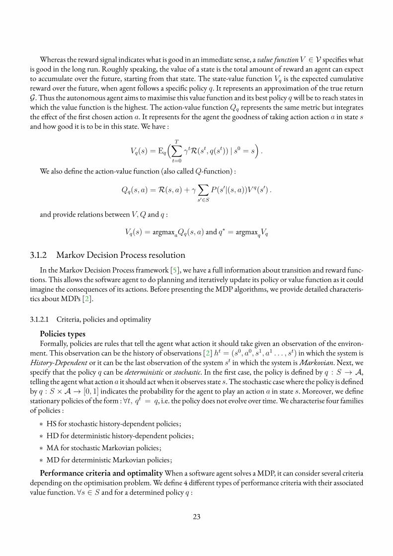
Whereas the reward signal indicates what is good in an immediate sense, a value functionV ∈ V specifies whatis good in the long run. Roughly speaking, the value of a state is the total amount of reward an agent can expectto accumulate over the future, starting from that state. The state-value function Vq is the expected cumulativereward over the future, when agent follows a specific policy q. It represents an approximation of the true returnG. Thus the autonomous agent aims tomaximise this value function and its best policy q will be to reach states inwhich the value function is the highest. The action-value functionQq represents the same metric but integratesthe effect of the first chosen action a. It represents for the agent the goodness of taking action action a in state sand how good it is to be in this state. We have :

Vq(s) = Eq

( T∑t=0

γtR(st, q(st)) | s0 = s).

We also define the action-value function (also calledQ-function) :

Qq(s, a) = R(s, a) + γ∑s′∈S

P (s′|(s, a))V q(s′) .

and provide relations between V,Q and q :

Vq(s) = argmaxaQq(s, a) and q∗ = argmaxqVq

3.1.2 Markov Decision Process resolutionIn theMarkovDecision Process framework [5], we have a full information about transition and reward func-

tions. This allows the software agent to do planning and iteratively update its policy or value function as it couldimagine the consequences of its actions. Before presenting theMDP algorithms, we provide detailed characteris-tics about MDPs [2].

3.1.2.1 Criteria, policies and optimality

Policies typesFormally, policies are rules that tell the agent what action it should take given an observation of the environ-

ment. This observation can be the history of observations [2] ht = (s0, a0, s1, a1 . . . , st) in which the system isHistory-Dependent or it can be the last observation of the system st in which the system isMarkovian. Next, wespecify that the policy q can be deterministic or stochastic. In the first case, the policy is defined by q : S → A,telling the agentwhat actiona it should actwhen it observes state s. The stochastic casewhere the policy is definedby q : S ×A → [0, 1] indicates the probability for the agent to play an action a in state s. Moreover, we definestationary policies of the form :∀t, qt = q, i.e. the policy does not evolve over time.We characterise four familiesof policies :

∗ HS for stochastic history-dependent policies ;∗ HD for deterministic history-dependent policies ;∗ MA for stochastic Markovian policies ;∗ MD for deterministic Markovian policies ;

Performance criteria and optimalityWhen a software agent solves aMDP, it can consider several criteriadepending on the optimisation problem.We define 4 different types of performance criteria with their associatedvalue function. ∀s ∈ S and for a determined policy q :

23

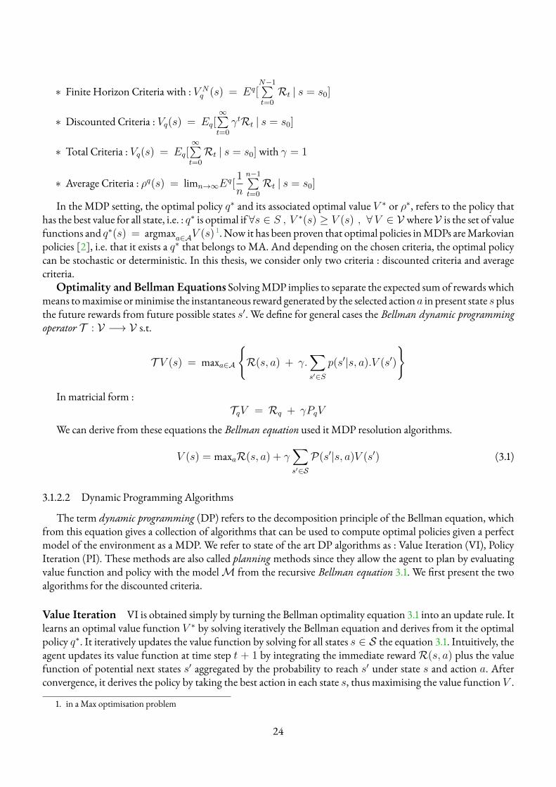
∗ Finite Horizon Criteria with : V Nq (s) = Eq[

N−1∑t=0

Rt | s = s0]

∗ Discounted Criteria : Vq(s) = Eq[∞∑t=0

γtRt | s = s0]

∗ Total Criteria : Vq(s) = Eq[∞∑t=0

Rt | s = s0] with γ = 1

∗ Average Criteria : ρq(s) = limn→∞Eq[

1

n

n−1∑t=0

Rt | s = s0]

In the MDP setting, the optimal policy q∗ and its associated optimal value V ∗ or ρ∗, refers to the policy thathas the best value for all state, i.e. : q∗ is optimal if ∀s ∈ S , V ∗(s) ≥ V (s) , ∀V ∈ V whereV is the set of valuefunctions and q∗(s) = argmaxa∈AV (s) 1. Now it has been proven that optimal policies inMDPs areMarkovianpolicies [2], i.e. that it exists a q∗ that belongs to MA. And depending on the chosen criteria, the optimal policycan be stochastic or deterministic. In this thesis, we consider only two criteria : discounted criteria and averagecriteria.

Optimality and Bellman Equations SolvingMDP implies to separate the expected sum of rewards whichmeans tomaximise orminimise the instantaneous reward generated by the selected action a in present state s plusthe future rewards from future possible states s′. We define for general cases the Bellman dynamic programmingoperator T : V −→ V s.t.

T V (s) = maxa∈A

{R(s, a) + γ.

∑s′∈S

p(s′|s, a).V (s′)

}

In matricial form :TqV = Rq + γPqV

We can derive from these equations the Bellman equation used it MDP resolution algorithms.

V (s) = maxaR(s, a) + γ∑s′∈S

P(s′|s, a)V (s′) (3.1)

3.1.2.2 Dynamic Programming Algorithms

The term dynamic programming (DP) refers to the decomposition principle of the Bellman equation, whichfrom this equation gives a collection of algorithms that can be used to compute optimal policies given a perfectmodel of the environment as a MDP. We refer to state of the art DP algorithms as : Value Iteration (VI), PolicyIteration (PI). These methods are also called planning methods since they allow the agent to plan by evaluatingvalue function and policy with the modelM from the recursive Bellman equation 3.1. We first present the twoalgorithms for the discounted criteria.

Value Iteration VI is obtained simply by turning the Bellman optimality equation 3.1 into an update rule. Itlearns an optimal value function V ∗ by solving iteratively the Bellman equation and derives from it the optimalpolicy q∗. It iteratively updates the value function by solving for all states s ∈ S the equation 3.1. Intuitively, theagent updates its value function at time step t + 1 by integrating the immediate rewardR(s, a) plus the valuefunction of potential next states s′ aggregated by the probability to reach s′ under state s and action a. Afterconvergence, it derives the policy by taking the best action in each state s, thus maximising the value function V .

1. in a Max optimisation problem

24

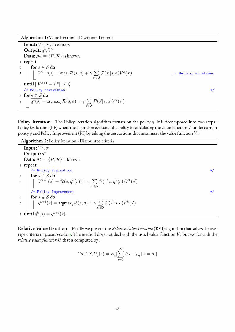
Algorithm 1:Value Iteration - Discounted criteriaInput: V 0, q0, ζ accuracyOutput: q∗, V ∗

Data:M = {P ,R} is known1 repeat2 for s ∈ S do3 V k+1(s) = maxaR(s, a) + γ

∑s′∈SP(s′|s, a)V k(s′) // Bellman equations

4 until ||V k+1 − V k|| ≤ ζ/* Policy derivation */

5 for s ∈ S do6 q∗(s) = argmaxaR(s, a) + γ

∑s′∈SP(s′|s, a)V k(s′)

Policy Iteration The Policy Iteration algorithm focuses on the policy q. It is decomposed into two steps :Policy Evaluation (PE)where the algorithm evaluates the policy by calculating the value functionV under currentpolicy q and Policy Improvement (PI) by taking the best actions that maximises the value function V .

Algorithm 2: Policy Iteration - Discounted criteriaInput: V 0, q0

Output: q∗

Data:M = {P ,R} is known1 repeat

/* Policy Evaluation */2 for s ∈ S do3 V k+1(s) = R(s, qk(s)) + γ

∑s′∈SP(s′|s, qk(s))V k(s′)

/* Policy Improvement */4 for s ∈ S do5 qk+1(s) = argmaxaR(s, a) + γ

∑s′∈SP(s′|s, a)V k(s′)

6 until qk(s) = qk+1(s)

Relative Value Iteration Finally we present the Relative Value Iteration (RVI) algorithm that solves the ave-rage criteria in pseudo-code 3. The method does not deal with the usual value function V , but works with therelative value function U that is computed by :

∀s ∈ S, Uq(s) = Eq[∞∑t=0

Rt − ρq | s = s0]

25

where ρq is the average gain under policy q. More details are provided for the study of average criteria in ChapterIV.

Algorithm 3:Relative Value Iteration - Average criteriaInput: U0 = 0, q0, ζ accuracyOutput: q∗, U∗, ρ∗

Data:M = {P ,R} is known1 repeat2 Choose s0 ∈ S3 ρk+1 = maxaR(s0, a) +

∑s′∈S

p(s′|s0, a)Uk(s′) // Average gain calculation

4 for s ∈ S do5 Uk+1(s) = maxa [R(s, a) + γ

∑s′∈S

p(s′|s, a)Uk(s′)]− ρk+1 // Average Bellman equations

6 until ||Uk+1 − Uk|| < ζ/* Policy derivation */

7 for s ∈ S do8 q∗(s) = argmaxa [R(s, a) + γ

∑s′∈S

p(s′|s, a)Uk(s′)]

3.2 Reinforcement learning

Let us define the environmentmodelM = {P ,R}. It is an object thatmimics the dynamics behaviour of theenvironment. Given a state s and an action a, it predicts the next state s′ with transition distribution P(s, a, .)and returns the rewardR(s, a). If the modelM is perfectly known, one can solve the problem by learning anoptimal policy with classical MDP solutions (see section 3.1.2). On the contrary, ifM is unknown, the problemcan be solvedwith reinforcement learning techniques that will be explain in this section. UnlikeMarkovDecisionProcess resolutionwithdynamic programming, theRLagent have to learn the optimal policy or value functionbyinteractingwith the environment in trial-and-errormode. In otherwords, theRL agent cannot performplanningcomputations and needs to collect data from environment interactions to update its policy or value function.The field of reinforcement learning can be decomposed into several branches that are displayed in section 3.2.2which provides the different classes of algorithms. We first provide the main intuition of reinforcement learningalgorithms, i.e. how the software agent can learn with collected experiences.

3.2.1 Main idea of Reinforcement LearningThe first idea borrowed from reinforcement learning techniques is theMonte Carlomethods,where the goal is

to perform experiences to estimates values. The goal in the RL paradigmwould be to estimate the value functionV q of a fixed policy qwith simulated trajectories and updating the value at the end of each trajectory. In a nutshell,the agent observes environment states s and decide to perform an action a given by its policy q(s). From thisinteraction, the agent collects a reward r and observes the new environment state s′. In a simulation, it wouldcollect a history of samples (s, a, r, s′) that it could use to learn the optimal value function or policy.

In a Monte Carlo simulation for RL, the agent will simulate trajectories k from each state s for a fixed periodT following policy q and will look at the cumulative sum of reward (or Return) obtained from that trajectoryRk(s). Then, it can approximate the value function V as :

26

∀s ∈ S , Vk+1(s) =R1(s) +R2(s) + . . .+Rk+1(s)

k + 1(3.2)

The essence of this method has led to a more modern approach called Temporal Di�erence (TD)-learning,which is the principalmethodology forQ-Learning algorithm. If one had to identify one idea as central and novelto reinforcement learning, it would undoubtedly be TD-learning. This method is a combination ofMonte Carloideas and DP ideas. Like Monte Carlo methods, TD methods can learn directly from raw experience without amodel of the environment’s dynamics. Like DP, TD methods update estimates based in part on other learnedestimates, without waiting for a final outcome. In other words, TD-learning methods are bootstrapping. We canstart from theMonte Carlo method equation to understand the TD-learning process and rewrite 3.2 :

∀s ∈ S , Vk+1(s) = Vk(s) +1

k + 1[Rk+1(s)− Vk(s)]

Which leads us to :

∀s ∈ S , Vk+1(s) = Vk(s) + α[Rk+1(s)− Vk(s)] (3.3)

where α is the learning rate.As said, TD-learning uses the incremental characteristics of dynamic programming and the trial characteristic

of Monte Carlo. We focus on discounted criteria with γ and present TD(0) or one-step TD which considersonly one time step. We depict next the reasoning that leads to the TD(0) update equation. If the value functionsestimates were exact, i.e. that it estimates perfectly the returnG, we would have the following :

V (st) = rt + γrt+1 + γ2rt+2 + . . .

V (st+1) = rt+1 + γrt+2 + γ2rt+3 + . . .

SoV (st+1) = rt + γV (st+1)

This leads to the one-step update equation for the value function, also called theWidrow-Ho� Equation :

V (st) = V (st) + α[rt + γV (st+1)− V (st)]︸ ︷︷ ︸TD-error

(3.4)

Like in Dynamic Programming, the value V (st) is updated with the value of the successor V (st+1) and withthe new reward received rt from the environment (see pseudo-code 4).Obviously,TDmethods have an advantageover DP methods in that they do not require a model of the environment, of its reward function and next-stateprobability distributions. The next most obvious advantage of TD methods over Monte Carlo methods is thatthey are naturally implemented in an on-line, fully incremental fashion and they do not need to wait until theend of an episode. Moreover, the convergence of TD-learning methods have been proven, i.e. that for any policy

27

q, TD(0) converges to Vq.

Algorithm 4:TD(0)-Learning - Discounted criteriaInput: V 0, q, α learning rate, γ discounted rateOutput: VqData:M = {P ,R} unknown/* Several simulation episodes */

1 for episodes do2 Initialise s = s0

/* Several steps until end of episode */3 for iterations do4 Select action a = q(s) and collect r and s′5 V (s) = V (s) + α[r + γV (s′)− V (s)]6 s← s′

This computational logic is present in most of the RL algorithms, that is the approximation of the return orcumulative sumof rewards which can be seen as a target for the value function or policy to update, in a supervisedlearning mode.

3.2.2 Taxonomy of RL algorithmsNow, to structure reinforcement learning techniques,we provide in this section an overviewofRL algorithms.

Our goal here is to highlight themost foundational design choices inRL algorithms about what to learn and howto learn it.

3.2.2.1 Model-free versus Model-based

One of themost important branching points in aRL algorithm is the question of whether the agent has accessto (or learns) the modelM of the environment. Algorithms which use a model are calledmodel-based, and thosethat don’t are calledmodel-free. Model-free techniques aim to update the policy or value function directly fromexperience without involving a model of the world, whereas the second one, on the contrary, works with themodel of the world. In model-based methods, the model can be given which bring us back to MDP resolution,or it can be learned by the agent from experiences. The agent is building an approximated model M = {P , R}to perform planning, i.e. update value function or policy.

Themain advantage of having amodel is that it allows the agent to plan by thinking ahead, seeing what wouldhappen for a set of possible choices, and explicitly deciding between its options. Agents can then integrate theresults of the planning into a learned policy. A particularly famous example of this approach is AlphaZero [129].While model-free methods renounce to the potential gains of sampling efficiency associated with using a model,they are easier to implement and tune. In the literature, model-free methods are more popular and have beenmore widely developed and tested than model-based methods for industrial applications.

3.2.2.2 Value-based versus Policy-based

Another critical branching point in a RL algorithm is the question of what to learn. The list of usual toolsincludes :

∗ policies, either stochastic or deterministic∗ action-value functions (Q-functions)

28

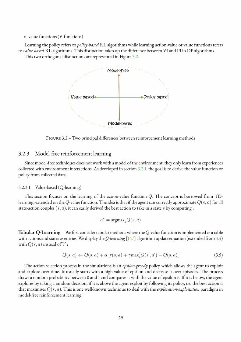
∗ value functions (V-functions)

Learning the policy refers to policy-based RL algorithms while learning action-value or value functions refersto value-based RL algorithms. This distinction takes up the difference between VI and PI in DP algorithms.

This two orthogonal distinctions are represented in Figure 3.2.

Figure 3.2 – Two principal differences between reinforcement learning methods

3.2.3 Model-free reinforcement learningSincemodel-free techniques does notworkwith amodel of the environment, they only learn from experiences

collected with environment interactions. As developed in section 3.2.1, the goal is to derive the value function orpolicy from collected data.

3.2.3.1 Value-based (Q-learning)

This section focuses on the learning of the action-value function Q. The concept is borrowed from TD-learning, extended on theQ-value function. The idea is that if the agent can correctly approximateQ(s, a) for allstate-action couples (s, a), it can easily derived the best action to take in a state s by computing :

a∗ = argmaxaQ(s, a)

Tabular Q-Learning We first consider tabularmethodswhere theQ-value function is implemented as a tablewith actions and states as entries.We display theQ-learning [147] algorithmupdate equation (extended from3.4)withQ(s, a) instead of V :

Q(s, a)← Q(s, a) + α [r(s, a) + γmax′aQ(s′, a′)−Q(s, a)] (3.5)

The action selection process in the simulations is an epsilon-greedy policy which allows the agent to exploitand explore over time. It usually starts with a high value of epsilon and decrease it over episodes. The processdraws a random probability between 0 and 1 and compares it with the value of epsilon ε. If it is below, the agentexplores by taking a random decision, if it is above the agent exploit by following its policy, i.e. the best action athat maximisesQ(s, a). This is one well-known technique to deal with the exploration-exploitation paradigm inmodel-free reinforcement learning.

29

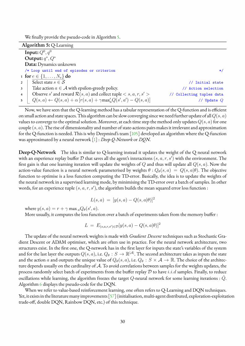
We finally provide the pseudo-code in Algorithm 5.

Algorithm 5:Q-LearningInput:Q0, q0

Output: q∗, Q∗

Data:Dynamics unknown/* Loop until end of episodes or criterion */

1 for e ∈ {1, . . . , Ne} do2 Select state s ∈ S // Initial state3 Take action a ∈ Awith epsilon-greedy policy. // Action selection4 Observe s′ and rewardR(s, a) and collect tuple< s, a, r, s′ > // Collecting tuples data5 Q(s, a)← Q(s, a) + α [r(s, a) + γmax′aQ(s′, a′)−Q(s, a)] // Update Q

Now, we have seen that the Q-learning method has a tabular representation of the Q-function and is efficienton small action and state spaces.This algorithmcanbe slow converging sinceweneed further update of allQ(s, a)values to converge to the optimal solution.Moreover, at each time step the method only updatesQ(s, a) for onecouple (s, a). The rise of dimensionality and number of state-actions pairsmakes it irrelevant and approximationfor the Q-function is needed. This is why Deepmind’s team [105] developed an algorithmwhere the Q-functionwas approximated by a neural network [1] :Deep-Q-Network orDQN.

Deep-Q-Network The idea is similar to Q-learning instead it updates the weight of the Q neural networkwith an experience replay bufferD that saves all the agent’s interactions (s, a, r, s′) with the environment. Thefirst gain is that one learning iteration will update the weights of Q and thus will update all Q(s, a). Now theaction-value function is a neural network parameterised by weights θ : Qθ(s, a) = Q(s, a|θ). The objectivefunction to optimise is a loss function computing the TD-error. Basically, the idea is to update the weights ofthe neural network in a supervised learning mode, by minimising the TD-error over a batch of samples. In otherwords, for an experience tuple (s, a, r, s′), the algorithm builds the mean squared error loss function :

L(s, a) = [y(s, a)−Q(s, a|θ)]2

where y(s, a) = r + γ max aQθ(s′, a).

More usually, it computes the loss function over a batch of experiments taken from the memory buffer :

L = E(s,a,r,s′)∈D[y(s, a)−Q(s, a|θ)]2

The update of the neural network weights is made withGradient Descent techniques such as Stochastic Gra-dient Descent or ADAM optimiser, which are often use in practice. For the neural network architecture, twostructures exist. In the first one, the Q-network has in the first layer for inputs the state’s variables of the systemand for the last layer the outputsQ(s, a), i.e.Qθ : S → R|A|. The second architecture takes as inputs the stateand the action a and outputs the unique value ofQθ(s, a), i.e. Qθ : S × A → R. The choice of the architec-ture depends usually on the cardinality ofA. To avoid correlations between samples for the weights updates, theprocess randomly select batch of experiments from the buffer replay D to have i.i.d samples. Finally, to reduceoscillations while learning, the algorithm freezes the target Q-neural network for some learning iterations : Q.Algorithm 6 displays the pseudo-code for the DQN.

When we refer to value-based reinforcement learning, one often refers to Q-Learning and DQN techniques.Yet, it exists in the literaturemany improvements [57] (initialisation,multi-agentdistributed, exploration-exploitationtrade-off, double DQN, RainbowDQN, etc.) of this technique.

30

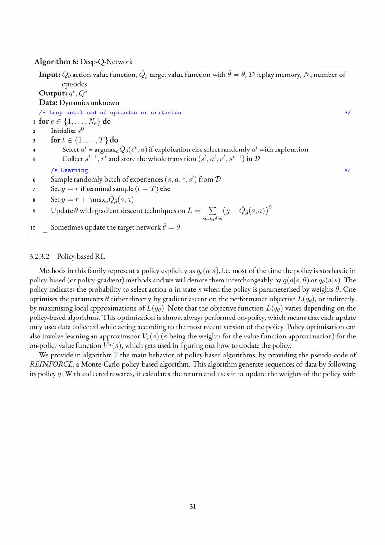
Algorithm 6:Deep-Q-Network

Input:Qθ action-value function, Qθ target value function with θ = θ,D replay memory,Ne number ofepisodes

Output: q∗, Q∗

Data:Dynamics unknown/* Loop until end of episodes or criterion */

1 for e ∈ {1, . . . , Ne} do2 Initialise s0

3 for t ∈ {1, . . . , T} do4 Select at = argmaxaQθ(s

t, a) if exploitation else select randomly at with exploration5 Collect st+1, rt and store the whole transition (st, at, rt, st+1) inD

/* Learning */6 Sample randomly batch of experiences (s, a, r, s′) fromD7 Set y = r if terminal sample (t = T ) else8 Set y = r + γmaxaQθ(s, a)

9 Update θ with gradient descent techniques on L =∑

samples

(y − Qθ(s, a)

)2

10 Sometimes update the target network θ = θ

3.2.3.2 Policy-based RL

Methods in this family represent a policy explicitly as qθ(a|s), i.e. most of the time the policy is stochastic inpolicy-based (or policy-gradient) methods and we will denote them interchangeably by q(a|s, θ) or qθ(a|s). Thepolicy indicates the probability to select action a in state s when the policy is parameterised by weights θ. Oneoptimises the parameters θ either directly by gradient ascent on the performance objective L(qθ), or indirectly,by maximising local approximations of L(qθ). Note that the objective function L(qθ) varies depending on thepolicy-based algorithms. This optimisation is almost always performed on-policy, which means that each updateonly uses data collected while acting according to the most recent version of the policy. Policy optimisation canalso involve learning an approximator Vφ(s) (φ being the weights for the value function approximation) for theon-policy value function V q(s), which gets used in figuring out how to update the policy.

We provide in algorithm 7 the main behavior of policy-based algorithms, by providing the pseudo-code ofREINFORCE, a Monte-Carlo policy-based algorithm. This algorithm generate sequences of data by followingits policy q. With collected rewards, it calculates the return and uses it to update the weights of the policy with

31

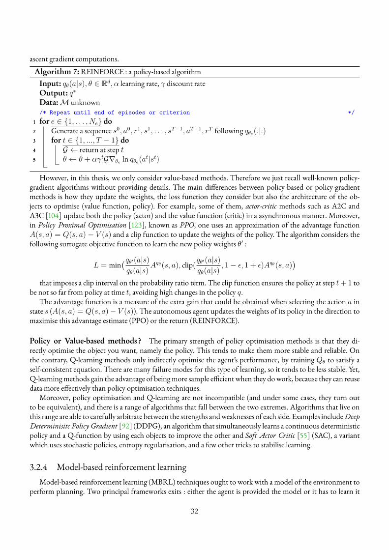
ascent gradient computations.

Algorithm 7:REINFORCE : a policy-based algorithmInput: qθ(a|s), θ ∈ Rd, α learning rate, γ discount rateOutput: q∗

Data:M unknown/* Repeat until end of episodes or criterion */

1 for e ∈ {1, . . . , Ne} do2 Generate a sequence s0, a0, r1, s1, . . . , sT−1, aT−1, rT following qθe(.|.)3 for t ∈ {1, ..., T − 1} do4 G ← return at step t5 θ ← θ + αγtG∇θe ln qθe(at|st)

However, in this thesis, we only consider value-based methods. Therefore we just recall well-known policy-gradient algorithms without providing details. The main differences between policy-based or policy-gradientmethods is how they update the weights, the loss function they consider but also the architecture of the ob-jects to optimise (value function, policy). For example, some of them, actor-critic methods such as A2C andA3C [104] update both the policy (actor) and the value function (critic) in a asynchronous manner. Moreover,in Policy Proximal Optimisation [123], known as PPO, one uses an approximation of the advantage functionA(s, a) = Q(s, a)− V (s) and a clip function to update the weights of the policy. The algorithm considers thefollowing surrogate objective function to learn the new policy weights θ′ :

L = min(qθ′(a|s)qθ(a|s)

Aqθ(s, a), clip(qθ′(a|s)qθ(a|s)

, 1− ε, 1 + ε)Aqθ(s, a))

that imposes a clip interval on the probability ratio term. The clip function ensures the policy at step t+ 1 tobe not so far from policy at time t, avoiding high changes in the policy q.

The advantage function is a measure of the extra gain that could be obtained when selecting the action a instate s (A(s, a) = Q(s, a)− V (s)). The autonomous agent updates the weights of its policy in the direction tomaximise this advantage estimate (PPO) or the return (REINFORCE).

Policy or Value-based methods ? The primary strength of policy optimisation methods is that they di-rectly optimise the object you want, namely the policy. This tends to make them more stable and reliable. Onthe contrary, Q-learning methods only indirectly optimise the agent’s performance, by training Qθ to satisfy aself-consistent equation. There are many failure modes for this type of learning, so it tends to be less stable. Yet,Q-learningmethods gain the advantage of beingmore sample efficient when they dowork, because they can reusedata more effectively than policy optimisation techniques.

Moreover, policy optimisation and Q-learning are not incompatible (and under some cases, they turn outto be equivalent), and there is a range of algorithms that fall between the two extremes. Algorithms that live onthis range are able to carefully arbitrate between the strengths andweaknesses of each side. Examples includeDeepDeterminisitc Policy Gradient [92] (DDPG), an algorithm that simultaneously learns a continuous deterministicpolicy and a Q-function by using each objects to improve the other and Soft Actor Critic [55] (SAC), a variantwhich uses stochastic policies, entropy regularisation, and a few other tricks to stabilise learning.

3.2.4 Model-based reinforcement learningModel-based reinforcement learning (MBRL) techniques ought to work with a model of the environment to

perform planning. Two principal frameworks exits : either the agent is provided the model or it has to learn it

32

from experience. We provide in this chapter familiarities about this class of RL methods and how it works : firsthow the agent can learn the world model and second how it can use the model for planning. The details aboutmodel-based algorithms (learning, planning, architectures) will be provided in Chapter V.

3.2.4.1 Learning the model

The usual scenario in reinforcement learning applications is that a ground-truth model of the environmentis not available to the agent. If an agent wants to use a model to operate planning techniques, it has to learn themodel purely from experience, which creates several challenges. The biggest challenge is that bias in themodel canbe exploited by the agent, resulting in an agentwhichperformswellwith respect to the learnedmodel, but behavessub-optimally (or super terribly) in the real environment. Learning the environment model is fundamentallyhard, as it can take lots of time to have a good approximation and can even fail. Since several years, some researchershave tempted to propose solutions for model learning in RL environments. Recall that the environment modelM should be an object that can predict the next state s′ and the reward r when the agent takes action a in states. We denote by M the approximated model that the agent learns from collected data. In some scenarios, theagent has to learn the dynamics of the environment P since the reward is hand-crafted by human knowledge orengineers and thus provided to the software agent. However, there are cases where the agent must also learn thereward. Chapter V and Chapter VI assume that the reward function is given to the agent and only the transitionprobabilities have to be approximated therefore we present works with this assumption.

What model to learn ? The first point asks what model the agent should learn. With environment interac-tions, the agent collects batch of one-step transition data (st, at, rt+1, st+1). There exist three principal types ofdynamics function [106] :∗ Forward model that predicts the new state st+1 at time t + 1 when the agent selected action a in state st attime t : (st, at)→ st+1 ;∗ Backward model that predicts the pair state-action (st, a) that led to the new state st+1 : (st, at)← st+1 ;∗ Inverse model that predictswhich action the agent should take tomove fromstatest to statest+1 : (st, st+1)←at

Model-based RL has mostly focused on forward models, and these will also be the main focus of our discussion,and investigated solutions in the thesis.

How to learn the model ? Now to estimate these forward models the agent has several mathematical toolsthat are nicely covered in the survey [106] and that will be detailed in Section 5.1 of Chapter V :∗ Non-parametricmethods that directly store and use the data to represent the model :

— Replay bu�ers [43, 133] : Replay buffers techniques are dealingwith deterministic modelswhere the col-lected tuple (s, a, r, s′) is kept inmemory (the replay buffer) for planning and updating value functionor policy. Basically, it acts as a predictor for couple (s, a)→ (r, s′) ;

— Approximate methods :Wemay also apply non-parametric and approximationmethodswhenwewantto be able to generalise information to similar states. In this context, we approximate the transitionmodel (s, a) → (r, s′) with approximated methods. For example, this can be done with neural net-works, linear approximation or Gaussian processes [145] that have became a popular non-parametricapproach.

∗ Parametricmethods, discussed in [56] :

33

— Exact tabular methods : For a discreteMDP (or a discretised version of a continuousMDPChapter V),a tabular method maintains a separate entry for every possible transition. For example, in a stochasticMDP (in which we need to learn a probability distribution), Sutton proposed a tabular maximum li-kelihood model [133] to estimate the probability of each possible transition (s, a) → s′ by countingoccurrences of visits in these couples (more details in Chapter V). Being able to learn this exact modelof the world allows first a safe planning and exploration thus the agent can train from simulated ex-periences. Moreover these methods are sample efficient in the sense that they require less interactionswith the environment to converge. However, they do not scale to high-dimensional problems, as thesize of the required table scales exponentially in the dimensionality of S (see Chapter V and ChapterVI).

— Approximate methods : The dynamic model function P can also be approximated by P , which willscale down thememory requirements and bemore feasible in large scale systems. Usually, the dynamicsapproximatorwill be parametric functions such as : Linear regression [8],Dynamic BayesianNetworks[26], Neural Networks [108], etc.

As we have seen, there are a variety of challenges and issues in model learning. In the next paragraph, we willdiscuss how this learned (or given) model may actually be used to act and learn in the environment.

3.2.4.2 Exploiting the model - Planning

The second branch of model-based RLmethods is about scenarios where the agent is given the environmentmodel or has learned the model. The main difference here is that in the former case the agent can directly doplanning based on the accuratemodel of theworldwhile in the latter case the agent needs to learn themodel frominteractions with the environment and then do some planning. This family of reinforcement learning algorithmswill be treated in Chapter IV, where it is assumed that the agent have a full knowledge of the environment modelM and in Chapter V, Chapter VI.

Model is given The very first case is about when the agent is provided beforehand the true model of theenvironmentM, including dynamics and reward functions. The very first techniques are the DP algorithms tosolve MDPs, described in section 3.1.2. Also more recent work such as AlphaZero [129] proposes model-basedRL withMonte Carlo Tree Search (MCTS) to master the game of Go.

Model is learned - Integration of Learning and Planning The scenariowhere the agent has learned themodel,or as we focus in this document the dynamics model P , differs from the case where the true model is provided.Indeed, the software agent have to use its updated model carefully, depending on its confidence in the learning.This raises several issues that are presented here but which will be detailed in the Background Section A.1 ofChapter V.

∗ Which first state to select for the planning : It exists several options to consider :

— A straightforward approach is to randomly select states throughout state space. This is the case of DPmethods which selects all possible states in a sweep. The major drawback of this approach is that itdoes not scale to high dimensional problems, since the total number of states grows exponentially inthe dimensionality of the state space ;

— We can also ensure that the agent only plans at reachable states by selecting previously visited states asstarting points. This is the case for Dyna architectures [133] (see Chapter V) ;

34

— Selecting visited states can also be improved with a prioritisation of the states. For example, to obtainan ordering over the reachable states, identifying their relevancy for a next planning update might besuitable. A good example is Prioritised Replay [122] (see Chapter V) which identifies state-action pairsthat likely need to be update, e.g. pairs with the highest TD-error ;

— Last, the agent can do planning directly from the current state it observes in the environment. Thisputs much emphasis at finding a better solution or more information in the region where we the agentcurrently operates.

∗ Trade-o� between time for collecting data and planning time : The challenge here is to define in the algorithmswhen the agent must do planning.

— Planning at each environment step : As an example, original Dyna architectures proposed by Sutton[133]makes up to a hundred planning steps after every real iteration in the environment, i.e. after eachtuple (s, a, r, s′) ;

— Planning after collecting several data :Theprincipal example is PILCO[36]which collects data in entireepisodes, and plans an entire solution after a set of new real transitions has been collected. This is alsoknown as Batch reinforcement learning where the agent plans after collecting a batch of experiments.

∗ How long should the planning phase last : The planning phase ismade of several iterations to browse the stateand action spaces for updating value functions or policies. One plan can be seen as an ’imagined’ simulationthat the agent can roll from the learned model. Two principal points emerge : how large the agent shouldbrowse the state space (or start a new planned simulation), known as breadth and how deep the plan shouldbe, known as depth. We detail below the two points and summarises it in Figure 3.3.

— Breadth of the plan to decide how large the agent browse the state space : Original model-based RLmethods usually consider a breadth of size 1 to sample single transitions from the model and applyingmodel-free updates, e.g. Dyna architectures. Very recent works integrate this reasoning in modernmodel-free techniques : e.g. withDDPG [70]. An othermore flexible example is AlphaZero [129]withMCTSmethod that deals with adaptive breadth sizes depending on the tree arms. Last techniques areDP algorithms such as VI and PI [5] that consider a breadth of full state space size, updating the valuefunction and the policy for all state s ∈ S for a depth of one, with recursive equation from time tto time t + 1. This is also the case forMDP online techniques [74], [27] where the agent ought toapproximate reward and transition matrices with a tabular maximum likelihood model [133]. Withthe learned model, it can do planning by solving the underlying MDP. These two algorithms will bepresented in Chapter V since they will be treated and influenced our work.

— Depth of the plan to decide how deep the agent plans. Original Dyna algorithms [133] considered adepth of size 1 (and breadth of size 1), i.e. the agent supplementary updates the couple (s, a) with thecollected data (s, a, r, s′). In the context ofDyna, [60] shows that plans longer than depth 1 give betterlearning performance. Finally, PILCO [36] proposes to plan until it terminates (final state, endingcondition).

Also note that the learning process can be done Online and Offline :∗ Online planning : planning is done just before executing an action in a given state s, i.e. that planning derivesthe policy q(s) for the given state s for example by evaluating V (s) only for this state ;∗ Offline planning : solves the problem offline for all possible states (e.g. Value Iteration), therefore derivingthe whole policy q(s) ∀s ∈ S.

35

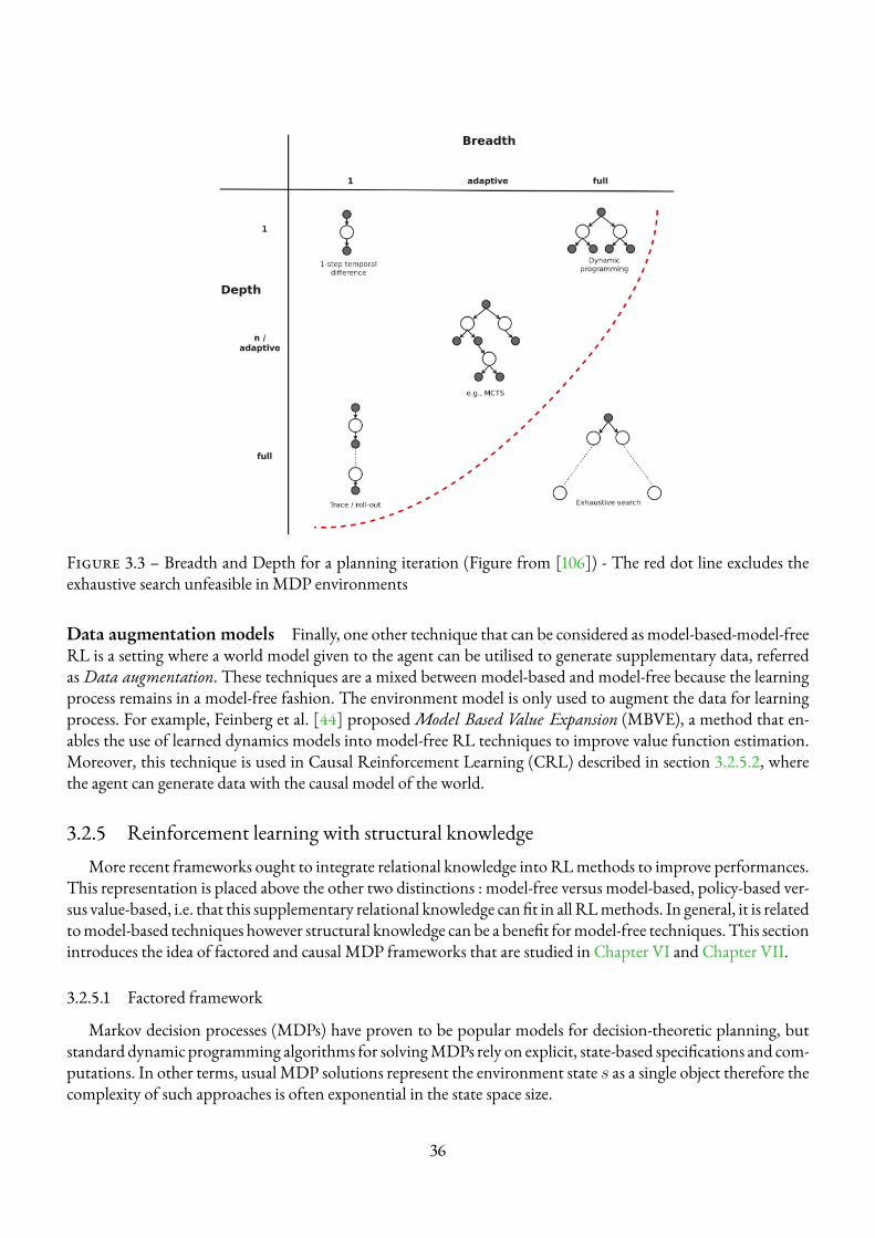
Figure 3.3 – Breadth and Depth for a planning iteration (Figure from [106]) - The red dot line excludes theexhaustive search unfeasible in MDP environments

Data augmentation models Finally, one other technique that can be considered as model-based-model-freeRL is a setting where a world model given to the agent can be utilised to generate supplementary data, referredasData augmentation. These techniques are a mixed between model-based and model-free because the learningprocess remains in a model-free fashion. The environment model is only used to augment the data for learningprocess. For example, Feinberg et al. [44] proposedModel Based Value Expansion (MBVE), a method that en-ables the use of learned dynamics models into model-free RL techniques to improve value function estimation.Moreover, this technique is used in Causal Reinforcement Learning (CRL) described in section 3.2.5.2, wherethe agent can generate data with the causal model of the world.

3.2.5 Reinforcement learning with structural knowledgeMore recent frameworks ought to integrate relational knowledge into RLmethods to improve performances.

This representation is placed above the other two distinctions : model-free versus model-based, policy-based ver-sus value-based, i.e. that this supplementary relational knowledge can fit in all RLmethods. In general, it is relatedtomodel-based techniques however structural knowledge can be a benefit formodel-free techniques. This sectionintroduces the idea of factored and causal MDP frameworks that are studied in Chapter VI and Chapter VII.

3.2.5.1 Factored framework

Markov decision processes (MDPs) have proven to be popular models for decision-theoretic planning, butstandard dynamic programming algorithms for solvingMDPs rely on explicit, state-based specifications and com-putations. In other terms, usual MDP solutions represent the environment state s as a single object therefore thecomplexity of such approaches is often exponential in the state space size.

36

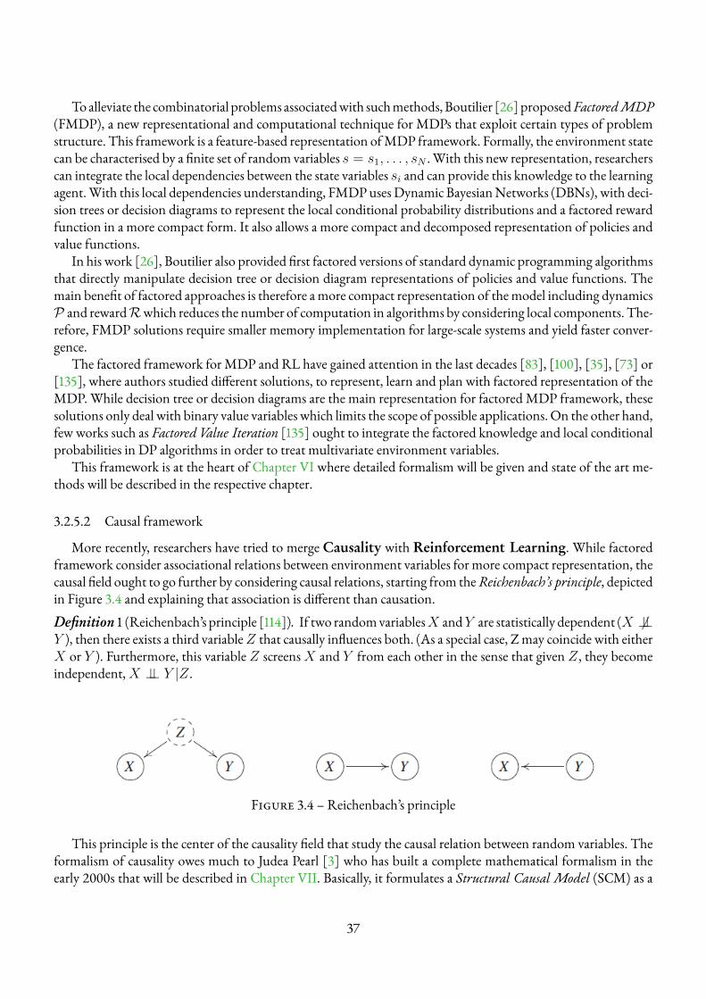
Toalleviate the combinatorial problems associatedwith suchmethods,Boutilier [26]proposedFactoredMDP(FMDP), a new representational and computational technique for MDPs that exploit certain types of problemstructure. This framework is a feature-based representation ofMDP framework. Formally, the environment statecan be characterised by a finite set of random variables s = s1, . . . , sN . With this new representation, researcherscan integrate the local dependencies between the state variables si and can provide this knowledge to the learningagent.With this local dependencies understanding, FMDPuses Dynamic BayesianNetworks (DBNs), with deci-sion trees or decision diagrams to represent the local conditional probability distributions and a factored rewardfunction in a more compact form. It also allows a more compact and decomposed representation of policies andvalue functions.

In his work [26], Boutilier also provided first factored versions of standard dynamic programming algorithmsthat directly manipulate decision tree or decision diagram representations of policies and value functions. Themain benefit of factored approaches is therefore amore compact representation of themodel including dynamicsP and rewardRwhich reduces the number of computation in algorithms by considering local components. The-refore, FMDP solutions require smaller memory implementation for large-scale systems and yield faster conver-gence.

The factored framework for MDP and RL have gained attention in the last decades [83], [100], [35], [73] or[135], where authors studied different solutions, to represent, learn and plan with factored representation of theMDP. While decision tree or decision diagrams are the main representation for factored MDP framework, thesesolutions only deal with binary value variables which limits the scope of possible applications. On the other hand,few works such as Factored Value Iteration [135] ought to integrate the factored knowledge and local conditionalprobabilities in DP algorithms in order to treat multivariate environment variables.

This framework is at the heart of Chapter VI where detailed formalism will be given and state of the art me-thods will be described in the respective chapter.

3.2.5.2 Causal framework

More recently, researchers have tried to merge Causality with Reinforcement Learning. While factoredframework consider associational relations between environment variables for more compact representation, thecausal field ought to go further by considering causal relations, starting from theReichenbach’s principle, depictedin Figure 3.4 and explaining that association is different than causation.Definition 1 (Reichenbach’s principle [114]). If two randomvariablesX andY are statistically dependent (X 6⊥⊥Y ), then there exists a third variableZ that causally influences both. (As a special case, Zmay coincide with eitherX or Y ). Furthermore, this variable Z screensX and Y from each other in the sense that given Z , they becomeindependent,X ⊥⊥ Y |Z .

Figure 3.4 – Reichenbach’s principle

This principle is the center of the causality field that study the causal relation between random variables. Theformalism of causality owes much to Judea Pearl [3] who has built a complete mathematical formalism in theearly 2000s that will be described in Chapter VII. Basically, it formulates a Structural Causal Model (SCM) as a

37

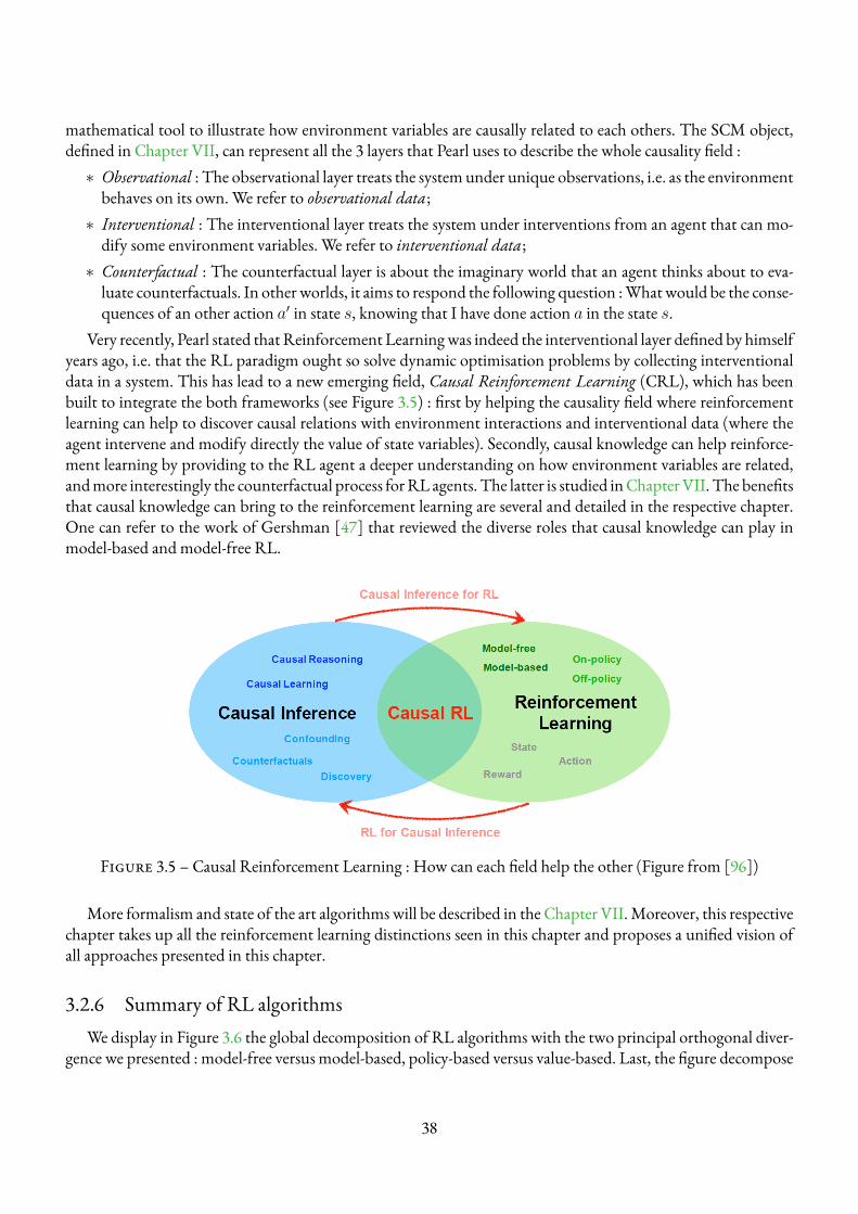
mathematical tool to illustrate how environment variables are causally related to each others. The SCM object,defined in Chapter VII, can represent all the 3 layers that Pearl uses to describe the whole causality field :∗ Observational : The observational layer treats the systemunder unique observations, i.e. as the environmentbehaves on its own. We refer to observational data ;∗ Interventional : The interventional layer treats the system under interventions from an agent that can mo-dify some environment variables. We refer to interventional data ;∗ Counterfactual : The counterfactual layer is about the imaginary world that an agent thinks about to eva-luate counterfactuals. In other worlds, it aims to respond the following question :Whatwould be the conse-quences of an other action a′ in state s, knowing that I have done action a in the state s.

Very recently, Pearl stated thatReinforcement Learningwas indeed the interventional layer defined by himselfyears ago, i.e. that the RL paradigm ought so solve dynamic optimisation problems by collecting interventionaldata in a system. This has lead to a new emerging field, Causal Reinforcement Learning (CRL), which has beenbuilt to integrate the both frameworks (see Figure 3.5) : first by helping the causality field where reinforcementlearning can help to discover causal relations with environment interactions and interventional data (where theagent intervene and modify directly the value of state variables). Secondly, causal knowledge can help reinforce-ment learning by providing to the RL agent a deeper understanding on how environment variables are related,andmore interestingly the counterfactual process forRL agents. The latter is studied inChapterVII. The benefitsthat causal knowledge can bring to the reinforcement learning are several and detailed in the respective chapter.One can refer to the work of Gershman [47] that reviewed the diverse roles that causal knowledge can play inmodel-based and model-free RL.

Figure 3.5 – Causal Reinforcement Learning : How can each field help the other (Figure from [96])

More formalism and state of the art algorithms will be described in the Chapter VII.Moreover, this respectivechapter takes up all the reinforcement learning distinctions seen in this chapter and proposes a unified vision ofall approaches presented in this chapter.

3.2.6 Summary of RL algorithmsWe display in Figure 3.6 the global decomposition of RL algorithms with the two principal orthogonal diver-

gence we presented : model-free versus model-based, policy-based versus value-based. Last, the figure decompose

38

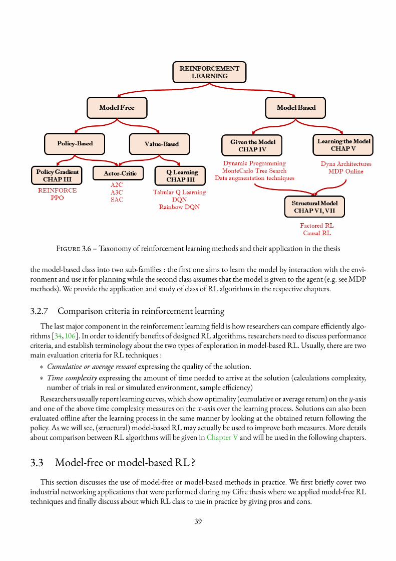
Figure 3.6 – Taxonomy of reinforcement learning methods and their application in the thesis

the model-based class into two sub-families : the first one aims to learn the model by interaction with the envi-ronment and use it for planning while the second class assumes that themodel is given to the agent (e.g. seeMDPmethods). We provide the application and study of class of RL algorithms in the respective chapters.

3.2.7 Comparison criteria in reinforcement learningThe last major component in the reinforcement learning field is how researchers can compare efficiently algo-

rithms [34, 106]. In order to identify benefits of designedRL algorithms, researchers need to discuss performancecriteria, and establish terminology about the two types of exploration in model-based RL. Usually, there are twomain evaluation criteria for RL techniques :∗ Cumulative or average reward expressing the quality of the solution.∗ Time complexity expressing the amount of time needed to arrive at the solution (calculations complexity,number of trials in real or simulated environment, sample efficiency)

Researchers usually report learning curves,which showoptimality (cumulative or average return) on the y-axisand one of the above time complexity measures on the x-axis over the learning process. Solutions can also beenevaluated offline after the learning process in the same manner by looking at the obtained return following thepolicy. As we will see, (structural) model-based RLmay actually be used to improve both measures. More detailsabout comparison between RL algorithms will be given in Chapter V and will be used in the following chapters.

3.3 Model-free or model-based RL?This section discusses the use of model-free or model-based methods in practice. We first briefly cover two

industrial networking applications that were performed during my Cifre thesis where we applied model-free RLtechniques and finally discuss about which RL class to use in practice by giving pros and cons.

39

3.3.1 Industrial networking applications

3.3.1.1 Grid of Beams

Wireless network coverage is defined as the extent of the area towhich thewireless signals are transmitted. Thecoverage is beam-based in 5G networks, not cell based. There is no cell-level reference channel from where thecoverage of the cell could be measured. Instead, each cell has one or multiple Synchronisation Signal Block Beam(SSB) beams. In legacy systems, SSB beams are static, or semi-static, always pointing to the same direction. Theyform a grid of beams covering the whole cell area. The UE (user equipment) searches for andmeasure the beams,maintaining a set of candidate beams. The candidate set of beams may contain beams from multiple cells. Themetrics measured are RSRP (Reference Signal Received Power), RSRQ (Reference Signal Received Quality),RSSI (Received Signal Strength Indicator) for each beam, that tells how good the received signal is for the UEs.Therefore there is a need to optimise the set of candidate beams that will maximise the coverage for the UEs. Weperformed a feasibility study of Deep RL techniques (DQN) in this networking problem that can be seen as acombinatorial optimisation problem. The main finding was that the DQN was outperformed by other classicaloptimisation techniques such as submodular optimisation and local search algorithms. The major issue of theDQN was its convergence time. One of the conclusions of this work is that if we have knowledge of the model(dynamics, reward function) then we must use it for offline planning and optimisation algorithms.

3.3.1.2 PDCPData Split

We also applied Deep RL techniques to an other networking use-case : PDCP (Packet Data Convergence Pro-tocol) Data Split in Dual Connectivity (DC) scenario. The PDCP layer handles transfer of user data, header com-pression, sequence numbering, duplication detection, packet duplication, etc. For the sake of describing the DCsolution, we consider an LTE scenario and adopt the LTE terminology.WithDC, aUE is simultaneously connec-ted to two different base stations : amaster eNB (MeNB) and a secondary eNB (SeNB). TheMeNB and the SeNBare connected via a non-ideal backhaul and operate on different carrier frequencies.

We were interested in optimising how to split the Packet Data Units (PDUs) sent by the UEs in the network,i.e. in which path the PDU should be forwarded to optimise latency and avoid overall congestion. In this context,we do not have a perfect modelling of the environment (dynamics and reward which is difficult tomeasure in realtime). Moreover, the action space for a learning agent is relatively simple since it only has very few choices (whereto send incoming PDUs). For this scenario, Deep RL methods were able to improve existing SoTA techniquesimplemented in practice, demonstrating real gain of applying model-free RL techniques.

3.3.2 Thesis position and overview of model-free versus model-based techniquesFirst of all, let us remind pros and cons for both model-free and model-based RLmethods.

— Model-free :— Pros : Computationally less complex and needs no accurate representation of the environment in order

to be effective.— Cons : Actual experiences need to be gathered in order for training, which makes exploration more

dangerous. Cannot carry an explicit plan of how environmental dynamics affects the system, especiallyin response to an action previously taken.

— Model-based :— Pros : Safe to plan exploration and can train from simulated experiences. Moreover they are sample

efficient in the sense that they require less interactions with the environment to converge.

40

— Cons : The learning agent is only as good as the model learnt. Sometimes this becomes a bottleneck,as the model becomes surprisingly tricky to learn. Finally, model-based methods are computationallymore complex than model-free methods.

In general, most of the reinforcement learning applications appear to bemodel-free techniques whether in theliterature or in industrial applications, mainly because of its ease of implementation and consideration.However,convergence problems are often mentioned when applying model-free techniques and this is simply because theautonomous agent should explore infinitely many times all the state-action pairs to obtain a good evaluation ofthe value function and the policy. Nevertheless, we have seen in practice but also for general use-cases that if wehave some information about the environment model, researchers should investigate this knowledge to buildor assess optimisation methods. The goal of this thesis is to evaluate and propose model-based reinforcementlearning techniques to accelerate the convergence and provide the agent with supplementary knowledge, in aCloud resource allocation use-case. It is believed that providing the model to the autonomous agent seems tobe a major benefit that should be integrated in its knowledge and that researches on model-based RL industrialapplications should be investigated. Chapter IV treats the scenario where the agent is given the modelM, andcan be also solutions to employ after the learning of the environmentmodel. Chapter V treats the scenario whereM, specially the dynamics P is unknown but the agent tries to approximate the dynamics model to performplanning. Chapter VI andChapter VII aremodel-based reinforcement learning proposal with factored and causalknowledgeof the environment.The latter can also treat complex environmentswith confounders andunobservedvariables which can be a huge issue in model-free techniques that will learn biased policy or value functions.

41

PART II

MODEL-BASEDAPPROACHES FOR CLOUDRESOURCE ALLOCATION

42

CHAPTER 4

MARKOVDECISION PROCESS ORHEURISTICS : HOWTOCOMPUTE AUTO-SCALINGHYSTERESIS POLICIES INQUEUING

SYSTEMSWITHKNOWNMODEL

The contributions of this chapter have been published in [139, 141] respectively :∗ Thomas Tournaire, Hind Castel-Taleb, Emmanuel Hyon. Generating optimal thresholds in a hysteresisqueue : a cloud application. In 27th IEEE International Symposium on the Modeling, Analysis, and Simu-lation of Computer and Telecommunication Systems (MASCOTS 19), 2019.∗ Thomas Tournaire, Hind Castel-Taleb, Emmanuel Hyon. Optimal control policies for resource alloca-tion in the Cloud : comparison between Markov decision process and heuristic approaches. In CoRRabs/2104.14879 (2021), 2021.

4.1 IntroductionThis chapter considers that the agent is provided the truemodel of the environmentM therefore its scope falls

into the classGiven the model of Figure 3.6.We consider a cost-aware approach and propose a global expected costconsidering different costs : associated with the performance requirements defined in a Service Level Agreement(SLA) and associated with energy consumption. We want to compute the optimal policy of activation and deac-tivation of the servers according to the queue occupation. In this chapter we studymodels in which the structureof the policy is of hysteresis form. However, assuming the policy has an hysteresis form is not sufficient to fullycharacterise the optimal policy. We have to determine the concrete values of thresholds. For this aim, there existtwo modelling approaches which correspond to two major streams in the literature. The first one expresses theproblem into a model of deterministic optimisation problem. This is done by using the average value of the costscomputed by stationary distribution of a CTMC (Continuous TimeMarkov Chains). Such an approach is oftenused in the field of inventory management for base stock policies [146] or reliable servers [149]. The second oneexpresses the problem under aMDP (MarkovDecision Process) model with structured polices and computes theoptimal one. But, although they are the most widely used for threshold computation, the efficiency of these twoapproaches are not assessed very carefully for the computation of single thresholds by level [6]. Especially, this hadnever been done for hysteresis policies. Fewworks focused on the optimality of hysteresis policy for cloudmodels[151] but, up to our knowledge, none on the threshold computation. Determining which is the best promisingapproach and which is the best model to choose in a practical use is thus an important point which is addressed

43

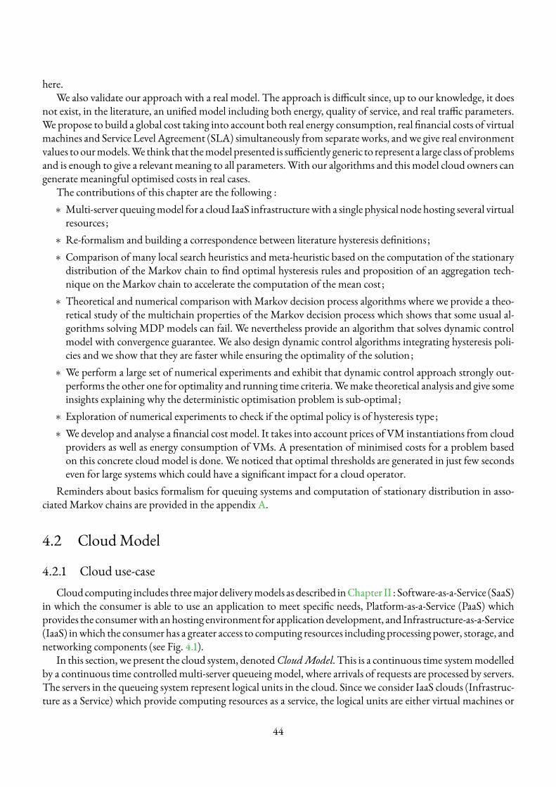
here.We also validate our approach with a real model. The approach is difficult since, up to our knowledge, it does

not exist, in the literature, an unified model including both energy, quality of service, and real traffic parameters.We propose to build a global cost taking into account both real energy consumption, real financial costs of virtualmachines and Service Level Agreement (SLA) simultaneously from separate works, andwe give real environmentvalues to ourmodels.We think that themodel presented is sufficiently generic to represent a large class of problemsand is enough to give a relevant meaning to all parameters.With our algorithms and this model cloud owners cangenerate meaningful optimised costs in real cases.

The contributions of this chapter are the following :∗ Multi-server queuingmodel for a cloud IaaS infrastructurewith a single physical node hosting several virtualresources ;∗ Re-formalism and building a correspondence between literature hysteresis definitions ;∗ Comparison of many local search heuristics and meta-heuristic based on the computation of the stationarydistribution of the Markov chain to find optimal hysteresis rules and proposition of an aggregation tech-nique on the Markov chain to accelerate the computation of the mean cost ;∗ Theoretical and numerical comparison with Markov decision process algorithms where we provide a theo-retical study of the multichain properties of the Markov decision process which shows that some usual al-gorithms solving MDP models can fail. We nevertheless provide an algorithm that solves dynamic controlmodel with convergence guarantee. We also design dynamic control algorithms integrating hysteresis poli-cies and we show that they are faster while ensuring the optimality of the solution;∗ We perform a large set of numerical experiments and exhibit that dynamic control approach strongly out-performs the other one for optimality and running time criteria.Wemake theoretical analysis and give someinsights explaining why the deterministic optimisation problem is sub-optimal ;∗ Exploration of numerical experiments to check if the optimal policy is of hysteresis type ;∗ We develop and analyse a financial cost model. It takes into account prices of VM instantiations from cloudproviders as well as energy consumption of VMs. A presentation of minimised costs for a problem basedon this concrete cloud model is done. We noticed that optimal thresholds are generated in just few secondseven for large systems which could have a significant impact for a cloud operator.

Reminders about basics formalism for queuing systems and computation of stationary distribution in asso-ciatedMarkov chains are provided in the appendix A.

4.2 CloudModel

4.2.1 Cloud use-caseCloud computing includes threemajor deliverymodels as described inChapter II : Software-as-a-Service (SaaS)

in which the consumer is able to use an application to meet specific needs, Platform-as-a-Service (PaaS) whichprovides the consumerwith anhosting environment for applicationdevelopment, and Infrastructure-as-a-Service(IaaS) inwhich the consumer has a greater access to computing resources including processing power, storage, andnetworking components (see Fig. 4.1).

In this section, we present the cloud system, denotedCloudModel. This is a continuous time systemmodelledby a continuous time controlledmulti-server queueingmodel, where arrivals of requests are processed by servers.The servers in the queueing system represent logical units in the cloud. Since we consider IaaS clouds (Infrastruc-ture as a Service) which provide computing resources as a service, the logical units are either virtual machines or

44

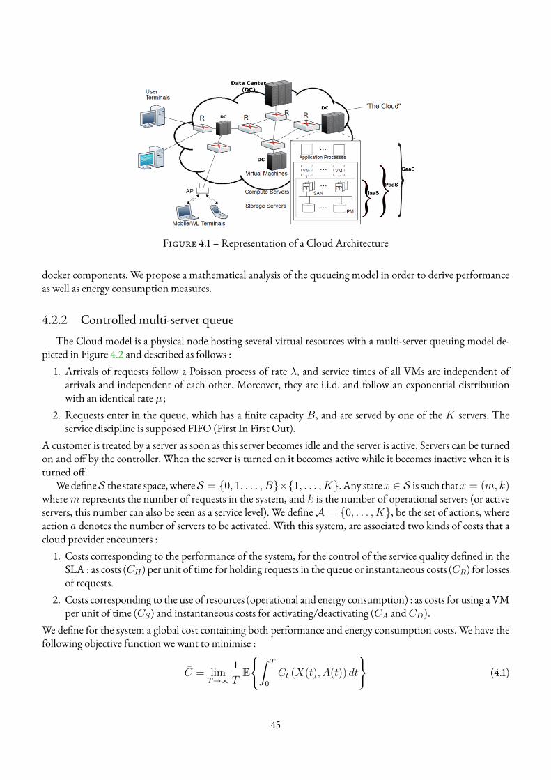
Figure 4.1 – Representation of a Cloud Architecture

docker components. We propose a mathematical analysis of the queueing model in order to derive performanceas well as energy consumption measures.

4.2.2 Controlled multi-server queueThe Cloud model is a physical node hosting several virtual resources with a multi-server queuing model de-

picted in Figure 4.2 and described as follows :1. Arrivals of requests follow a Poisson process of rate λ, and service times of all VMs are independent ofarrivals and independent of each other. Moreover, they are i.i.d. and follow an exponential distributionwith an identical rate µ ;

2. Requests enter in the queue, which has a finite capacity B, and are served by one of the K servers. Theservice discipline is supposed FIFO (First In First Out).

A customer is treated by a server as soon as this server becomes idle and the server is active. Servers can be turnedon and off by the controller. When the server is turned on it becomes active while it becomes inactive when it isturned off.

WedefineS the state space,whereS = {0, 1, . . . , B}×{1, . . . , K}. Any statex ∈ S is such thatx = (m, k)wherem represents the number of requests in the system, and k is the number of operational servers (or activeservers, this number can also be seen as a service level). We defineA = {0, . . . , K}, be the set of actions, whereaction a denotes the number of servers to be activated. With this system, are associated two kinds of costs that acloud provider encounters :

1. Costs corresponding to the performance of the system, for the control of the service quality defined in theSLA : as costs (CH) per unit of time for holding requests in the queue or instantaneous costs (CR) for lossesof requests.

2. Costs corresponding to the use of resources (operational and energy consumption) : as costs for using a VMper unit of time (CS) and instantaneous costs for activating/deactivating (CA andCD).

We define for the system a global cost containing both performance and energy consumption costs. We have thefollowing objective function we want to minimise :

C = limT→∞

1

TE

{∫ T

0

Ct (X(t), A(t)) dt

}(4.1)

45

whereA(t) is the action taken at time t (it is possible that nothing was performed) andCt(X(t), A(t)) is the costthat is charged over time when the state isX(t) and actionA(t) is performed. This problem can be solved in twodifferent ways based on two different models : using a Continuous Time Markov Chain to solve deterministicoptimisation problem (see section 4.3.2) or using Semi Markov Decision Processes (see section 4.6).

Figure 4.2 –Multi-server queuing system

4.3 Hysteresis policies and hysteresis queuing model

4.3.1 Hysteresis policiesAdecision rule is amapping from some information set to some action. A policy is a sequence of decision rules

η = (q0, q1, q2, . . .). The most general set of policies is that of history-dependent randomised policies, but theclassical results on average infinite-horizon, time-homogeneousMarkovian optimal control [5] allow us to focuson stationary Markov Deterministic Policies. Such policies are characterised by a single, deterministic decisionrule whichmaps the current state to an action.We thus consider themapping q fromS toA such that q(x) = a.

All along the chapter we restrict our attentionwith a special form of policies : the hysteresis policies. Neverthe-less, there are few homogeneities between definitions of hysteresis policies in the literature and we provide herea correspondence between them. Indeed, it can refer to policies defined with double thresholds (especially whenK = 2), or to a restrictive definition when Markov chains are used. We follow the works of [58, 78] to presentan unified treatment of hysteresis.

Hysteresis policies with multiple activations We assume in this part that the decision rule is a mappingfrom the state to a number of active servers q(m, k) = k1 with k1 ∈ [1, . . . , K]. Several servers can be activatedor deactivated to pass from k to k1 active servers.Definition 2 (Double threshold policies [58, 78]). We call double threshold policy a stationary policy such thatthe decision rule q(m, k) is increasing in both of its arguments and is defined by a sequence of thresholds suchthat for any k and k1 in [1, K] we have :

q(m, k) = k1 when `k1(k) ≤ m < `k1+1(k) ,

where `k1(k) = min{m : q(m, k) ≥ k1}. Thisminimum is∞ if the set is empty. For allk, we also fix `K+1(k) =∞ and `1(k) = 0 (since at least one server must be active).

A monotone hysteresis policy is a special case of double threshold policy.

46

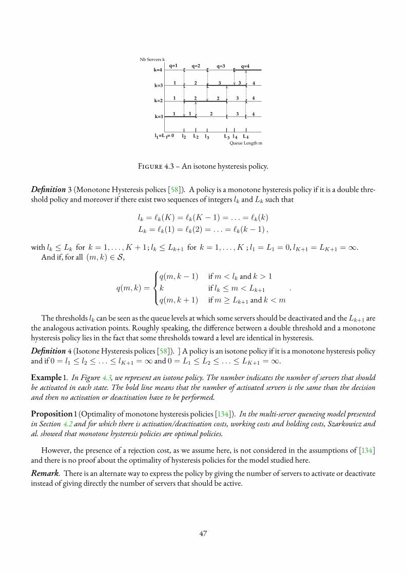
l =L = 01 1 l2 l3L2 L3 l 4 L 4

1

1

1

q=2

2

2 2

q=3 q=4

3 32

3

3 4

4

4

q=1

1

k=4

k=3

k=2

k=1

Nb Servers k

Queue Length m

Figure 4.3 – An isotone hysteresis policy.

Definition 3 (Monotone Hysteresis polices [58]). A policy is a monotone hysteresis policy if it is a double thre-shold policy and moreover if there exist two sequences of integers lk and Lk such that

lk = `k(K) = `k(K − 1) = . . . = `k(k)

Lk = `k(1) = `k(2) = . . . = `k(k − 1) ,

with lk ≤ Lk for k = 1, . . . , K + 1 ; lk ≤ Lk+1 for k = 1, . . . , K ; l1 = L1 = 0, lK+1 = LK+1 =∞.And if, for all (m, k) ∈ S ,

q(m, k) =

q(m, k − 1) ifm < lk and k > 1

k if lk ≤ m < Lk+1

q(m, k + 1) ifm ≥ Lk+1 and k < m

.

The thresholds lk can be seen as the queue levels at which some servers should be deactivated and theLk+1 arethe analogous activation points. Roughly speaking, the difference between a double threshold and a monotonehysteresis policy lies in the fact that some thresholds toward a level are identical in hysteresis.Definition 4 (IsotoneHysteresis polices [58]). ] A policy is an isotone policy if it is a monotone hysteresis policyand if 0 = l1 ≤ l2 ≤ . . . ≤ lK+1 =∞ and 0 = L1 ≤ L2 ≤ . . . ≤ LK+1 =∞.

Example 1. In Figure 4.3, we represent an isotone policy. The number indicates the number of servers that shouldbe activated in each state. The bold line means that the number of activated servers is the same than the decisionand then no activation or deactivation have to be performed.

Proposition 1 (Optimality of monotone hysteresis policies [134]). In the multi-server queueing model presentedin Section 4.2 and for which there is activation/deactivation costs, working costs and holding costs, Szarkowicz andal. showed that monotone hysteresis policies are optimal policies.

However, the presence of a rejection cost, as we assume here, is not considered in the assumptions of [134]and there is no proof about the optimality of hysteresis policies for the model studied here.Remark. There is an alternate way to express the policy by giving the number of servers to activate or deactivateinstead of giving directly the number of servers that should be active.

47

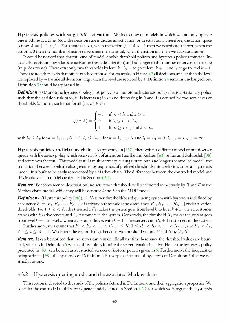
Hysteresis policies with single VM activation We focus now on models in which we can only operateone machine at a time. Now the decision rule indicates an activation or deactivation. Therefore, the action spaceis nowA = {−1, 0, 1}. For a state (m, k), when the action q ∈ A is−1 then we deactivate a server, when theaction is 0 then the number of active servers remains identical, when the action is 1 then we activate a server.

It could be noticed that, for this kind of model, double threshold policies and hysteresis policies coincide. In-deed, the decision now relates to activation (resp. deactivation) and no longer to the number of servers to activate(resp. deactivate). There exist only two thresholds by level k :Lk+1 to go to level k+ 1, and lk to go to level k−1.There are no other levels that can be reached from k. For example, in Figure 4.3 all decisions smaller than the levelare replaced by−1while all decisions larger than the level are replaced by 1. Definition 4 remains unchanged, butDefinition 3 should be rephrased in :Definition 5 (Monotone hysteresis policy). A policy is a monotone hysteresis policy if it is a stationary policysuch that the decision rule q(m, k) is increasing inm and decreasing in k and if is defined by two sequences ofthresholds lk and Lk such that for all (m, k) ∈ S :

q(m, k) =

−1 ifm < lk and k > 1

0 if lk ≤ m < Lk+1

1 ifm ≥ Lk+1 and k < m

,

with lk ≤ Lk for k = 1, . . . , K + 1 ; lk ≤ Lk+1 for k = 1, . . . , K and l1 = L1 = 0 ; lK+1 = LK+1 =∞.

Hysteresis policies and Markov chain As presented in [137], there exists a different model of multi-serverqueuewith hysteresis policywhich received a lot of attention (see Ibe andKeilson [63] or Lui andGolubchik [98]and references therein). Thismodel is still amulti-server queueing systembut is no longer a controlledmodel : thetransitions between levels are also governed by sequences of prefixed thresholds this is why it is called an hysteresismodel. It is built to be easily represented by a Markov chain. The differences between the controlled model andthis Markov chain model are detailed in Section 4.6.3.Remark. For convenience, deactivation and activation thresholds will be denoted respectively byR andF in theMarkov chain model, while they will be denoted l and L in the MDPmodel.Definition 6 (Hysteresis policy [98]). AK-server threshold-based queueing systemwith hysteresis is defined bya sequenceF = [F1, F2, . . . , FK−1] of activation thresholds and a sequence [R1, R2, . . . , RK−1] of deactivationthresholds. For 1 ≤ k < K , the thresholdFk makes the system goes from level k to level k+ 1when a customerarrives with k active servers and Fk customers in the system. Conversely, the thresholdRk makes the system goesfrom level k + 1 to level k when a customer leaves with k + 1 active servers andRk + 1 customers in the system.

Furthermore, we assume that F1 < F2 < . . . < FK−1 ≤ K , 1 ≤ R1 < R2 < . . . < RK−1, andRk < Fk,∀ 1 ≤ k ≤ K − 1. We denote the vector that gathers the two threshold vectors F andR by [F,R].Remark. It can be noticed that, no server can remain idle all the time here since the threshold values are boun-ded, whereas in Definition 5 when a threshold is infinite the server remains inactive. Hence the hysteresis policypresented in [63] can be seen as a restricted version of isotone policies given in 5. Furthermore, the inequalitiesbeing strict in [98], the hysteresis of Definition 6 is a very specific case of hysteresis of Definition 5 that we callstrictly isotone.

4.3.2 Hysteresis queuing model and the associatedMarkov chainThis section is devoted to the study of the policies defined inDefinition 6 and their aggregation properties.We

consider the controlled multi-server queue model defined in Section 4.2.2 for which we integrate the hysteresis

48

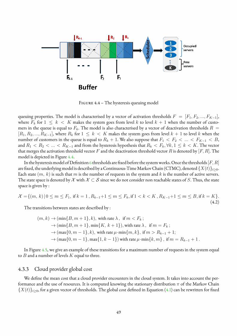
Figure 4.4 – The hysteresis queuing model

queuing properties. The model is characterised by a vector of activation thresholds F = [F1, F2, ..., FK−1],where Fk for 1 ≤ k < K makes the system goes from level k to level k + 1 when the number of custo-mers in the queue is equal to Fk. The model is also characterised by a vector of deactivation thresholds R =[R1, R2, ..., RK−1], where Rk for 1 ≤ k < K makes the system goes from level k + 1 to level k when thenumber of customers in the queue is equal to Rk + 1. We also suppose that F1 < F2 < ... < FK−1 < B,and R1 < R2 < ... < RK−1 and from the hysteresis hypothesis that Rk < Fk, ∀k, 1 ≤ k < K . The vectorthat merges the activation threshold vector F and the deactivation threshold vectorR is denoted by [F,R]. Themodel is depicted in Figure 4.4.

In thehysteresismodel ofDefinition6 thresholds are fixedbefore the systemworks.Once the thresholds [F,R]are fixed, the underlyingmodel is described by aContinuous-TimeMarkovChain (CTMC), denoted {X(t)}t≥0.Each state (m, k) is such thatm is the number of requests in the system and k is the number of active servers.The state space is denoted byX withX ⊂ S since we do not consider non reachable states of S. Thus, the statespace is given by :

X ={(m, k) |0 ≤ m ≤ F1, if k = 1 , Rk−1+1 ≤ m ≤ Fk, if 1 < k < K ,RK−1+1 ≤ m ≤ B, if k = K}.(4.2)

The transitions between states are described by :

(m, k)→ (min{B,m+ 1}, k), with rate λ , ifm < Fk ;

→ (min{B,m+ 1},min{K, k + 1}),with rate λ , ifm = Fk ;

→ (max{0,m− 1}, k), with rateµ·min{m, k}, ifm > Rk−1 + 1;

→ (max{0,m− 1},max{1, k − 1})with rateµ·min{k,m} , ifm = Rk−1 + 1 .

In Figure 4.5, we give an example of these transitions for a maximum number of requests in the system equaltoB and a number of levelsK equal to three.

4.3.3 Cloud provider global costWe define the mean cost that a cloud provider encounters in the cloud system. It takes into account the per-

formance and the use of resources. It is computed knowing the stationary distribution π of the Markov Chain{X(t)}t≥0, for a given vector of thresholds. The global cost defined in Equation (4.1) can be rewritten for fixed

49

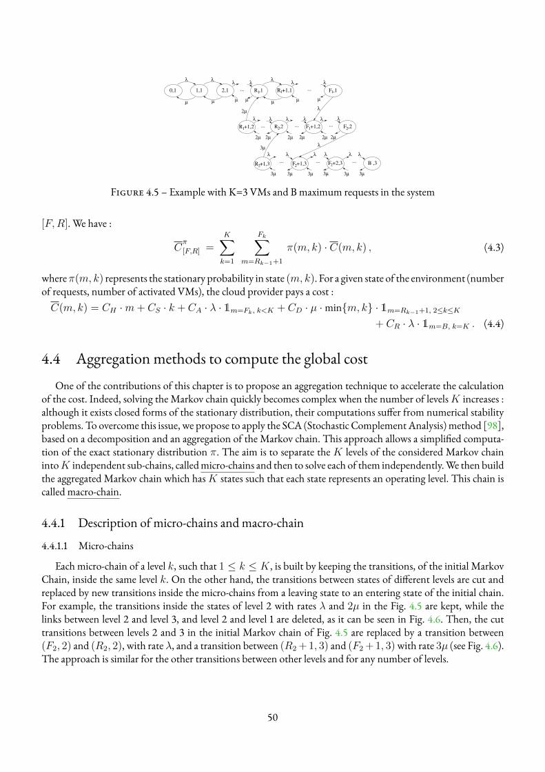
10,1 1,1 2,1 R ,1 R +1,1... ... F ,1

R +1,2 ... ...1

...F +1,2R ,21

... ... ...B ,3R +1,3 F +1,3 F +2,3

2 2

λ λ

λ

µ

λλ λ λ λ

λ λ λλ λ λ

λ

2µ 2µ 2µ2µ

2µ

3µ

3µ 3µ 3µ 3µ 3µ 3µ

1

2

1

F ,22 2

µµ µ µ µ µ

2µ

λ λ λλ

λ

λ

2µ

Figure 4.5 – Example with K=3 VMs and B maximum requests in the system

[F,R]. We have :

Cπ

[F,R] =K∑k=1

Fk∑m=Rk−1+1

π(m, k) · C(m, k) , (4.3)

whereπ(m, k) represents the stationary probability in state (m, k). For a given state of the environment (numberof requests, number of activated VMs), the cloud provider pays a cost :C(m, k) = CH ·m+ CS · k + CA · λ · 1m=Fk, k<K + CD · µ ·min{m, k} · 1m=Rk−1+1, 2≤k≤K

+ CR · λ · 1m=B, k=K . (4.4)

4.4 Aggregation methods to compute the global costOne of the contributions of this chapter is to propose an aggregation technique to accelerate the calculation

of the cost. Indeed, solving the Markov chain quickly becomes complex when the number of levelsK increases :although it exists closed forms of the stationary distribution, their computations suffer from numerical stabilityproblems. To overcome this issue, we propose to apply the SCA (Stochastic Complement Analysis) method [98],based on a decomposition and an aggregation of the Markov chain. This approach allows a simplified computa-tion of the exact stationary distribution π. The aim is to separate theK levels of the considered Markov chainintoK independent sub-chains, calledmicro-chains and then to solve each of them independently.We then buildthe aggregated Markov chain which hasK states such that each state represents an operating level. This chain iscalled macro-chain.

4.4.1 Description of micro-chains and macro-chain

4.4.1.1 Micro-chains

Each micro-chain of a level k, such that 1 ≤ k ≤ K , is built by keeping the transitions, of the initial MarkovChain, inside the same level k. On the other hand, the transitions between states of different levels are cut andreplaced by new transitions inside the micro-chains from a leaving state to an entering state of the initial chain.For example, the transitions inside the states of level 2 with rates λ and 2µ in the Fig. 4.5 are kept, while thelinks between level 2 and level 3, and level 2 and level 1 are deleted, as it can be seen in Fig. 4.6. Then, the cuttransitions between levels 2 and 3 in the initial Markov chain of Fig. 4.5 are replaced by a transition between(F2, 2) and (R2, 2), with rate λ, and a transition between (R2 + 1, 3) and (F2 + 1, 3)with rate 3µ (see Fig. 4.6).The approach is similar for the other transitions between other levels and for any number of levels.

50

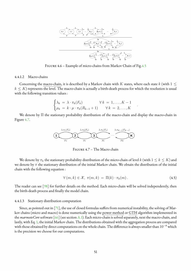
10,1 1,1 2,1 R ,1 R +1,1... ... F ,1

R +1,2 ... ...1

...F +1,2R ,21

... ... ...B ,3R +1,3 F +1,3 F +2,3

2 2

λ λ

µ

λλ λ λ λ

λ λ

2µ 2µ

3µ 3µ 3µ 3µ 3µ 3µ

1

2

1

F ,22 2

µ µ µ

2µ

λ λ

2µ

µ µµ

λ λ λ λ

λ

λ λλ λ

2µ 2µ

3µ

2µ

λ

Figure 4.6 – Example of micro-chains fromMarkov Chain of Fig.4.5

4.4.1.2 Macro-chains

Concerning the macro-chain, it is described by a Markov chain withK states, where each state k (with 1 ≤k ≤ K) represents the level. The macro-chain is actually a birth-death process for which the resolution is usualwith the following transition values :{

λk = λ · πk(Fk) ∀ k = 1, . . . , K − 1

µk = k · µ · πk(Rk−1 + 1) ∀ k = 2, . . . , K.

We denote by Π the stationary probability distribution of the macro-chain and display the macro-chain inFigure 4.7.

Figure 4.7 – TheMacro chain

We denote by πk the stationary probability distribution of the micro-chain of level k (with 1 ≤ k ≤ K) andwe denote by π the stationary distribution of the initial Markov chain. We obtain the distribution of the initialchain with the following equation :

∀ (m, k) ∈ X , π(m, k) = Π(k) · πk(m) . (4.5)

The reader can see [98] for further details on the method. Each micro-chain will be solved independently, thenthe birth-death process and finally the model chain.

4.4.1.3 Stationary distribution computation

Since, as pointed out in [71], the use of closed formulas suffers from numerical instability, the solving ofMar-kov chains (micro and macro) is done numerically using the power method or GTH algorithm implemented inthemarmoteCore software [66] (see sectionA.1). Eachmicro-chain is solved separately, next themacro-chain, andlastly, with Eq. 1, the initialMarkov chain. The distributions obtained with the aggregation process are comparedwith those obtained by direct computations on thewhole chain. The difference is always smaller than 10−8 whichis the precision we choose for our computations.

51

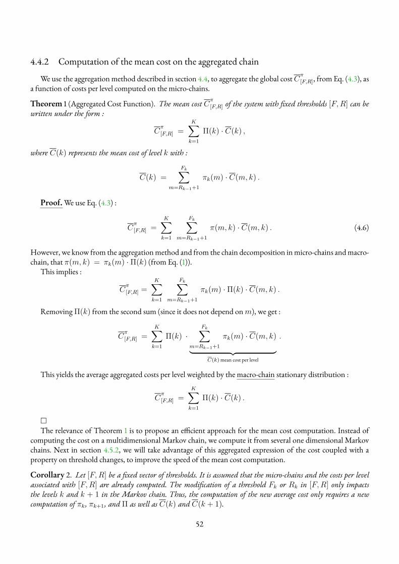
4.4.2 Computation of the mean cost on the aggregated chain

We use the aggregation method described in section 4.4, to aggregate the global costCπ

[F,R], from Eq. (4.3), asa function of costs per level computed on the micro-chains.

Theorem 1 (Aggregated Cost Function). The mean cost Cπ

[F,R] of the system with fixed thresholds [F,R] can bewritten under the form :

Cπ

[F,R] =K∑k=1

Π(k) · C(k) ,

where C(k) represents the mean cost of level k with :

C(k) =

Fk∑m=Rk−1+1

πk(m) · C(m, k) .

Proof.We use Eq. (4.3) :

Cπ

[F,R] =K∑k=1

Fk∑m=Rk−1+1

π(m, k) · C(m, k) . (4.6)

However, we know from the aggregationmethod and from the chain decomposition inmicro-chains andmacro-chain, that π(m, k) = πk(m) · Π(k) (from Eq. (1)).

This implies :

Cπ

[F,R] =K∑k=1

Fk∑m=Rk−1+1

πk(m) · Π(k) · C(m, k) .

Removing Π(k) from the second sum (since it does not depend onm), we get :

Cπ

[F,R] =K∑k=1

Π(k) ·Fk∑

m=Rk−1+1

πk(m) · C(m, k)

︸ ︷︷ ︸C(k)mean cost per level

.

This yields the average aggregated costs per level weighted by the macro-chain stationary distribution :

Cπ

[F,R] =K∑k=1

Π(k) · C(k) .

�The relevance of Theorem 1 is to propose an efficient approach for the mean cost computation. Instead of

computing the cost on a multidimensional Markov chain, we compute it from several one dimensional Markovchains. Next in section 4.5.2, we will take advantage of this aggregated expression of the cost coupled with aproperty on threshold changes, to improve the speed of the mean cost computation.

Corollary 2. Let [F,R] be a fixed vector of thresholds. It is assumed that the micro-chains and the costs per levelassociated with [F,R] are already computed. The modification of a threshold Fk or Rk in [F,R] only impactsthe levels k and k + 1 in the Markov chain. Thus, the computation of the new average cost only requires a newcomputation of πk, πk+1, and Π as well as C(k) and C(k + 1).

52

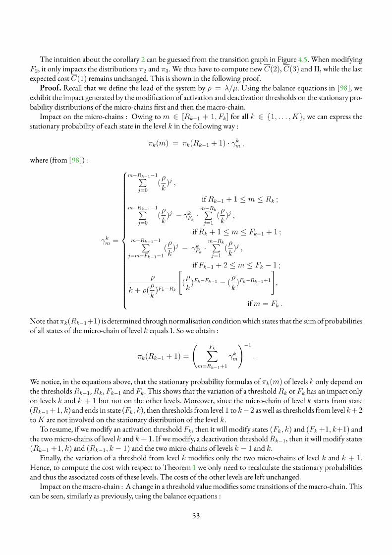
The intuition about the corollary 2 can be guessed from the transition graph in Figure 4.5. When modifyingF2, it only impacts the distributions π2 and π3. We thus have to compute newC(2),C(3) and Π, while the lastexpected costC(1) remains unchanged. This is shown in the following proof.

Proof. Recall that we define the load of the system by ρ = λ/µ. Using the balance equations in [98], weexhibit the impact generated by the modification of activation and deactivation thresholds on the stationary pro-bability distributions of the micro-chains first and then the macro-chain.

Impact on the micro-chains : Owing tom ∈ [Rk−1 + 1, Fk] for all k ∈ {1, . . . , K}, we can express thestationary probability of each state in the level k in the following way :

πk(m) = πk(Rk−1 + 1) · γkm ,

where (from [98]) :

γkm =

m−Rk−1−1∑j=0

(ρ

k)j ,

ifRk−1 + 1 ≤ m ≤ Rk ;m−Rk−1−1∑

j=0

(ρ

k)j − γkFk ·

m−Rk∑j=1

(ρ

k)j ,

ifRk + 1 ≤ m ≤ Fk−1 + 1 ;m−Rk−1−1∑j=m−Fk−1−1

(ρ

k)j − γkFk ·

m−Rk∑j=1

(ρ

k)j ,

if Fk−1 + 2 ≤ m ≤ Fk − 1 ;

ρ

k + ρ(ρ

k)Fk−Rk

[(ρ

k)Fk−Fk−1 − (

ρ

k)Fk−Rk−1+1

],

ifm = Fk .

Note thatπk(Rk−1+1) is determined throughnormalisation conditionwhich states that the sumof probabilitiesof all states of the micro-chain of level k equals 1. So we obtain :

πk(Rk−1 + 1) =

(Fk∑

m=Rk−1+1

γkm

)−1

.

We notice, in the equations above, that the stationary probability formulas of πk(m) of levels k only depend onthe thresholdsRk−1,Rk, Fk−1 and Fk. This shows that the variation of a thresholdRk or Fk has an impact onlyon levels k and k + 1 but not on the other levels. Moreover, since the micro-chain of level k starts from state(Rk−1 +1, k) and ends in state (Fk, k), then thresholds from level 1 to k−2 as well as thresholds from level k+2toK are not involved on the stationary distribution of the level k.

To resume, if we modify an activation thresholdFk, then it will modify states (Fk, k) and (Fk +1, k+1) andthe twomicro-chains of level k and k+ 1. If we modify, a deactivation thresholdRk−1, then it will modify states(Rk−1 +1, k) and (Rk−1, k − 1) and the two micro-chains of levels k − 1 and k.

Finally, the variation of a threshold from level k modifies only the two micro-chains of level k and k + 1.Hence, to compute the cost with respect to Theorem 1 we only need to recalculate the stationary probabilitiesand thus the associated costs of these levels. The costs of the other levels are left unchanged.

Impact on themacro-chain : A change in a threshold valuemodifies some transitions of themacro-chain. Thiscan be seen, similarly as previously, using the balance equations :

53

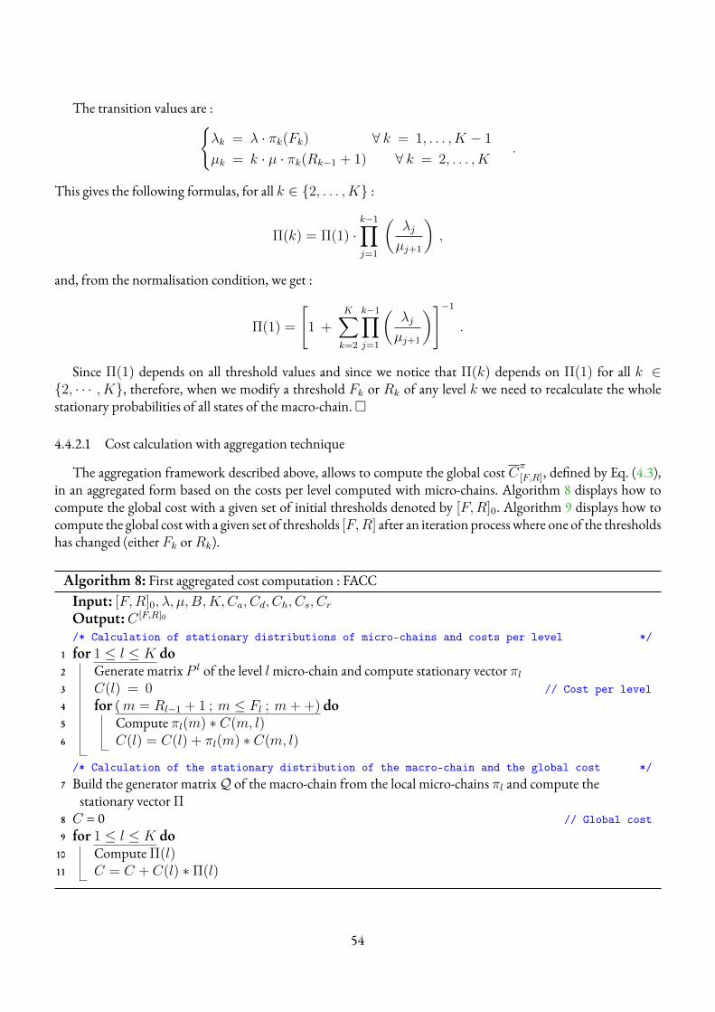
The transition values are :{λk = λ · πk(Fk) ∀ k = 1, . . . , K − 1

µk = k · µ · πk(Rk−1 + 1) ∀ k = 2, . . . , K.

This gives the following formulas, for all k ∈ {2, . . . , K} :

Π(k) = Π(1) ·k−1∏j=1

(λjµj+1

),

and, from the normalisation condition, we get :

Π(1) =

[1 +

K∑k=2

k−1∏j=1

(λjµj+1

)]−1

.

Since Π(1) depends on all threshold values and since we notice that Π(k) depends on Π(1) for all k ∈{2, · · · , K}, therefore, when we modify a threshold Fk or Rk of any level k we need to recalculate the wholestationary probabilities of all states of the macro-chain.�

4.4.2.1 Cost calculation with aggregation technique

The aggregation framework described above, allows to compute the global cost Cπ

[F,R], defined by Eq. (4.3),in an aggregated form based on the costs per level computed with micro-chains. Algorithm 8 displays how tocompute the global cost with a given set of initial thresholds denoted by [F,R]0. Algorithm 9 displays how tocompute the global cost with a given set of thresholds [F,R] after an iteration process where one of the thresholdshas changed (either Fk orRk).

Algorithm 8: First aggregated cost computation : FACCInput: [F,R]0, λ, µ,B,K,Ca, Cd, Ch, Cs, CrOutput:C [F,R]0

/* Calculation of stationary distributions of micro-chains and costs per level */1 for 1 ≤ l ≤ K do2 Generate matrix P l of the level lmicro-chain and compute stationary vector πl3 C(l) = 0 // Cost per level4 for (m = Rl−1 + 1 ; m ≤ Fl ; m+ +) do5 Compute πl(m) ∗ C(m, l)6 C(l) = C(l) + πl(m) ∗ C(m, l)

/* Calculation of the stationary distribution of the macro-chain and the global cost */7 Build the generator matrixQ of the macro-chain from the local micro-chains πl and compute the

stationary vector Π8 C = 0 // Global cost9 for 1 ≤ l ≤ K do

10 Compute Π(l)11 C = C + C(l) ∗ Π(l)

54

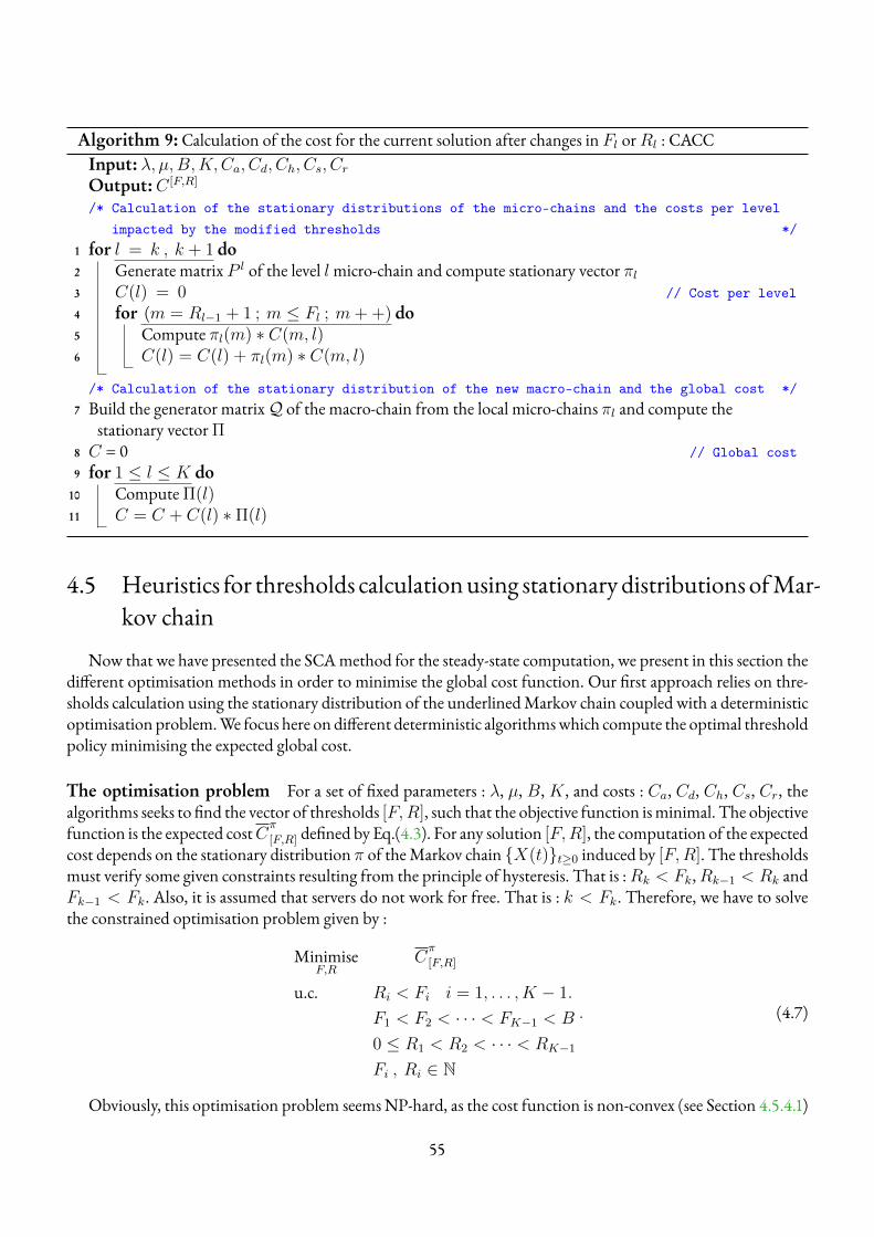
Algorithm 9: Calculation of the cost for the current solution after changes in Fl orRl : CACCInput: λ, µ,B,K,Ca, Cd, Ch, Cs, CrOutput:C [F,R]

/* Calculation of the stationary distributions of the micro-chains and the costs per levelimpacted by the modified thresholds */

1 for l = k , k + 1 do2 Generate matrix P l of the level lmicro-chain and compute stationary vector πl3 C(l) = 0 // Cost per level4 for (m = Rl−1 + 1 ; m ≤ Fl ; m+ +) do5 Compute πl(m) ∗ C(m, l)6 C(l) = C(l) + πl(m) ∗ C(m, l)

/* Calculation of the stationary distribution of the new macro-chain and the global cost */7 Build the generator matrixQ of the macro-chain from the local micro-chains πl and compute the

stationary vector Π8 C = 0 // Global cost9 for 1 ≤ l ≤ K do

10 Compute Π(l)11 C = C + C(l) ∗ Π(l)

4.5 Heuristics for thresholds calculationusing stationarydistributionsofMar-kov chain

Now that we have presented the SCAmethod for the steady-state computation, we present in this section thedifferent optimisation methods in order to minimise the global cost function. Our first approach relies on thre-sholds calculation using the stationary distribution of the underlinedMarkov chain coupled with a deterministicoptimisation problem.We focus here on different deterministic algorithmswhich compute the optimal thresholdpolicy minimising the expected global cost.

The optimisation problem For a set of fixed parameters : λ, µ, B,K , and costs : Ca, Cd, Ch, Cs, Cr, thealgorithms seeks to find the vector of thresholds [F,R], such that the objective function isminimal. The objectivefunction is the expected costCπ

[F,R] defined by Eq.(4.3). For any solution [F,R], the computation of the expectedcost depends on the stationary distribution π of theMarkov chain {X(t)}t≥0 induced by [F,R]. The thresholdsmust verify some given constraints resulting from the principle of hysteresis. That is :Rk < Fk,Rk−1 < Rk andFk−1 < Fk. Also, it is assumed that servers do not work for free. That is : k < Fk. Therefore, we have to solvethe constrained optimisation problem given by :

MinimiseF,R

Cπ

[F,R]

u.c. Ri < Fi i = 1, . . . , K − 1.

F1 < F2 < · · · < FK−1 < B

0 ≤ R1 < R2 < · · · < RK−1

Fi , Ri ∈ N

. (4.7)

Obviously, this optimisation problem seems NP-hard, as the cost function is non-convex (see Section 4.5.4.1)

55

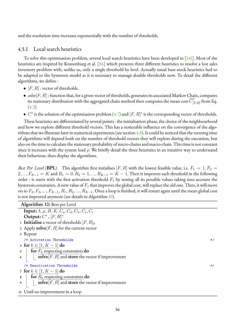
and the resolution time increases exponentially with the number of thresholds.

4.5.1 Local search heuristicsTo solve this optimisation problem, several local search heuristics have been developed in [141]. Most of the

heuristics are inspired by Kranenburg et al. [84] which presents three different heuristics to resolve a lost salesinventory problem with, unlike us, only a single threshold by level. Actually usual base-stock heuristics had tobe adapted to the hysteresis model as it is necessary to manage double thresholds now. To detail the differentalgorithms, we define :• [F,R] : vector of thresholds.• solve[F,R] : function that, for a given vector of thresholds, generates its associatedMarkovChain, computesits stationary distribution with the aggregated chain method then computes the mean costCπ

[F,R] from Eq.(4.3).• C∗ is the solution of the optimisation problem (4.7) and [F,R]∗ is the corresponding vector of thresholds.These heuristics are differentiated by several points : the initialisation phase, the choice of the neighbourhood

and how we explore different threshold vectors. This has a noticeable influence on the convergence of the algo-rithms that we illustrate later in numerical experiments (see section 4.8). It could be noticed that the running timeof algorithms will depend both on the number of threshold vectors they will explore during the execution, butalso on the time to calculate the stationary probability ofmicro-chains andmacro-chain. This time is not constantsince it increases with the system load ρ. We briefly detail the three heuristics in an intuitive way to understandtheir behaviour, then display the algorithms.

Best Per Level (BPL) This algorithm first initialises [F,R] with the lowest feasible value, i.e. F1 = 1, F2 =2, ..., FK−1 = K andR1 = 0, R2 = 1, ..., RK−1 = K − 1. Then it improves each threshold in the followingorder : it starts with the first activation threshold F1 by testing all its possible values taking into account thehysteresis constraints. A new value ofF1 that improves the global cost, will replace the old one. Then, it will moveon to F2, F3, ... , FK−1, R1, R2, ..., RK−1. Once a loop is finished, it will restart again until the mean global costis not improved anymore (see details in Algorithm 10).

Algorithm 10: Best per LevelInput: λ, µ,B,K,Ca, Cd, Ch, Cs, CrOutput:C∗ , [F,R]∗

1 Initialise a vector of thresholds [F,R]02 Apply solve[F,R] for the current vector3 Repeat/* Activation Thresholds */

4 for k ∈ [1, K − 1] do5 for Fk respecting constraints do6 solve[F,R] and store the vector if improvement

/* Deactivation Thresholds */7 for k ∈ [1, K − 1] do8 forRk respecting constraints do9 solve[F,R] and store the vector if improvement

10 Until no improvement in a loop

56

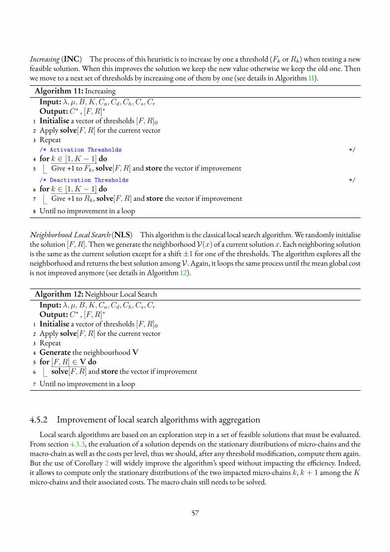
Increasing (INC) The process of this heuristic is to increase by one a threshold (Fk orRk) when testing a newfeasible solution. When this improves the solution we keep the new value otherwise we keep the old one. Thenwe move to a next set of thresholds by increasing one of them by one (see details in Algorithm 11).

Algorithm 11: IncreasingInput: λ, µ,B,K,Ca, Cd, Ch, Cs, CrOutput:C∗ , [F,R]∗

1 Initialise a vector of thresholds [F,R]02 Apply solve[F,R] for the current vector3 Repeat/* Activation Thresholds */

4 for k ∈ [1, K − 1] do5 Give +1 to Fk, solve[F,R] and store the vector if improvement/* Deactivation Thresholds */

6 for k ∈ [1, K − 1] do7 Give +1 toRk, solve[F,R] and store the vector if improvement8 Until no improvement in a loop

Neighborhood Local Search (NLS) This algorithm is the classical local search algorithm.We randomly initialisethe solution [F,R]. Thenwe generate the neighborhoodV(x) of a current solutionx. Each neighboring solutionis the same as the current solution except for a shift±1 for one of the thresholds. The algorithm explores all theneighborhood and returns the best solution amongV . Again, it loops the same process until themean global costis not improved anymore (see details in Algorithm 12).

Algorithm 12:Neighbour Local SearchInput: λ, µ,B,K,Ca, Cd, Ch, Cs, CrOutput:C∗ , [F,R]∗

1 Initialise a vector of thresholds [F,R]02 Apply solve[F,R] for the current vector3 Repeat4 Generate the neighbourhoodV5 for [F,R] ∈ V do6 solve[F,R] and store the vector if improvement7 Until no improvement in a loop

4.5.2 Improvement of local search algorithms with aggregationLocal search algorithms are based on an exploration step in a set of feasible solutions that must be evaluated.

From section 4.3.3, the evaluation of a solution depends on the stationary distributions of micro-chains and themacro-chain as well as the costs per level, thus we should, after any threshold modification, compute them again.But the use of Corollary 2 will widely improve the algorithm’s speed without impacting the efficiency. Indeed,it allows to compute only the stationary distributions of the two impacted micro-chains k, k + 1 among theKmicro-chains and their associated costs. The macro chain still needs to be solved.

57

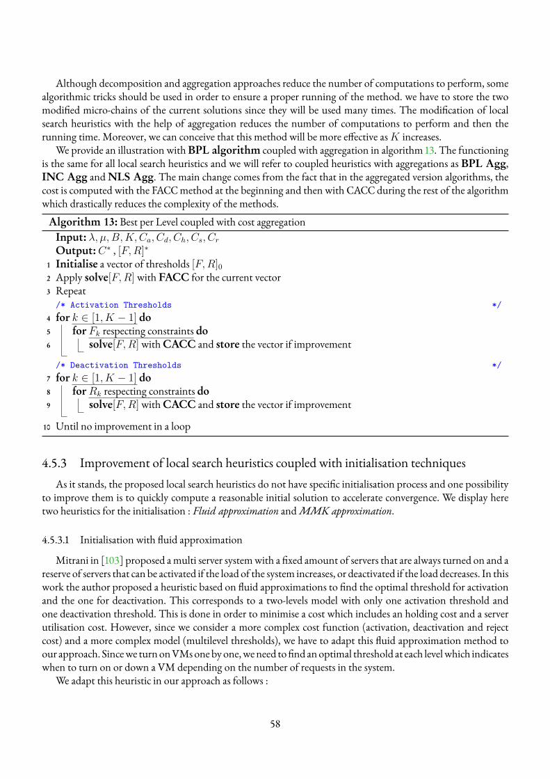
Although decomposition and aggregation approaches reduce the number of computations to perform, somealgorithmic tricks should be used in order to ensure a proper running of the method. we have to store the twomodified micro-chains of the current solutions since they will be used many times. The modification of localsearch heuristics with the help of aggregation reduces the number of computations to perform and then therunning time. Moreover, we can conceive that this method will be more effective asK increases.

We provide an illustration withBPL algorithm coupled with aggregation in algorithm 13. The functioningis the same for all local search heuristics and we will refer to coupled heuristics with aggregations as BPL Agg,INC Agg and NLS Agg. The main change comes from the fact that in the aggregated version algorithms, thecost is computed with the FACCmethod at the beginning and then with CACC during the rest of the algorithmwhich drastically reduces the complexity of the methods.

Algorithm 13: Best per Level coupled with cost aggregationInput: λ, µ,B,K,Ca, Cd, Ch, Cs, CrOutput:C∗ , [F,R]∗

1 Initialise a vector of thresholds [F,R]02 Apply solve[F,R] with FACC for the current vector3 Repeat/* Activation Thresholds */

4 for k ∈ [1, K − 1] do5 for Fk respecting constraints do6 solve[F,R] withCACC and store the vector if improvement

/* Deactivation Thresholds */7 for k ∈ [1, K − 1] do8 forRk respecting constraints do9 solve[F,R] withCACC and store the vector if improvement

10 Until no improvement in a loop

4.5.3 Improvement of local search heuristics coupled with initialisation techniquesAs it stands, the proposed local search heuristics do not have specific initialisation process and one possibility

to improve them is to quickly compute a reasonable initial solution to accelerate convergence. We display heretwo heuristics for the initialisation : Fluid approximation andMMK approximation.

4.5.3.1 Initialisation with fluid approximation

Mitrani in [103] proposed amulti server systemwith a fixed amount of servers that are always turned on and areserve of servers that can be activated if the load of the system increases, or deactivated if the load decreases. In thiswork the author proposed a heuristic based on fluid approximations to find the optimal threshold for activationand the one for deactivation. This corresponds to a two-levels model with only one activation threshold andone deactivation threshold. This is done in order to minimise a cost which includes an holding cost and a serverutilisation cost. However, since we consider a more complex cost function (activation, deactivation and rejectcost) and a more complex model (multilevel thresholds), we have to adapt this fluid approximation method toour approach. Sincewe turnonVMsonebyone,weneed to find anoptimal threshold at each levelwhich indicateswhen to turn on or down a VM depending on the number of requests in the system.

We adapt this heuristic in our approach as follows :

58

Deactivation Thresholds Similarly as [103],we decide to turn off virtualmachineswhenever they are unusedas we don’t want VMs to work for free. For the deactivation thresholds, we consider at each level k that thereserve is composed of only one virtual machine, since we have k VMs activated. This implies that we have k− 1VMs activated plus the reserve, which is exactly one VM here. Therefore, deactivating the reserve will lead toRk = k − 1.

Activation Thresholds Adding a newVMwill empty the queue faster and indeedwill improve theQoS, butwill deteriorate the energy part by adding operational costs. Letting unchanged the current number of activatedVMs will empty the queue in a slower time but will be less expensive regarding energy costs. In order to obtainactivation thresholds, we use a fluid approximation (inspired from [103]) to approximate if it is useful to turn ona new VM to empty the queue or not. We define by Ck(u) the approximated cost corresponding to k workingservers and u requests is the system :

Ck(u) =u

2· Bk(u) · Ch + k · Bk(u) · Cs + pk ·

λ

λ+ k · µ· Cr . (4.8)

The time until the queue is empty when there are u requests in the system, is defined by Bk(u). Assuming thequeue behaves like a deterministic fluid, the load would decrease at the rate of k · µ− λ and we get

Bk(u) =u

kµ− λunit of times .

The loss probability in level k is pk and is computed by approximating the loss probability of anM/M/1/Bqueue,with arrival rateλ, and service ratek·µ.Notice that (u·Ch·Bk(u))/2 represents thequeuing cost and Bk(u)·k·Csis the consumption cost of k active VMs.

The activation threshold Fk represents the smallest amount of requests u in the system, for which it is inter-esting to activate a new VM, i.e. the cost for k + 1 VMs activated plus the activation cost is lower than the costwith k VMs activated. At level k, we thus solve a computational problem to determine the activation thresholds.Precisely, we have to find the first u∈ N denoted by uk such that :

I(u) = Ck+1(u) + Ca − Ck(u) < 0 .

However, Bk(u) is relevant only when kµ − λ > 0, which intuitively means that the queue can be empty.Otherwise if λ ≥ kµ, we decide, in those cases, to fix the thresholds as low as possible, which is relevant becauseif the load is high, then one has to activate the VMs quickly to satisfy the QoS defined by the SLA. Finally, theoptimal activation thresholds are given by :

Fk =

{max {Fk−1 + 1,min{uk, B}} if λ < kµ

Rk + 1 if λ ≥ kµ.

59

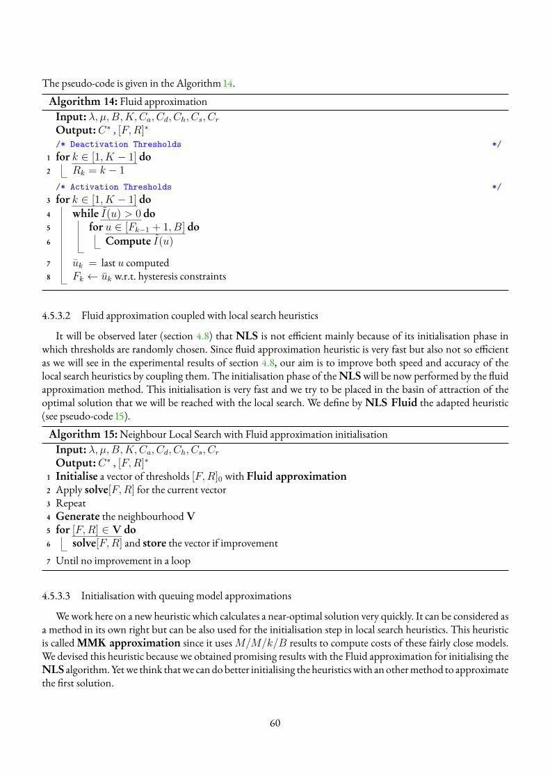
The pseudo-code is given in the Algorithm 14.

Algorithm 14: Fluid approximationInput: λ, µ,B,K,Ca, Cd, Ch, Cs, CrOutput:C∗ , [F,R]∗

/* Deactivation Thresholds */1 for k ∈ [1, K − 1] do2 Rk = k − 1

/* Activation Thresholds */3 for k ∈ [1, K − 1] do4 while I(u) > 0 do5 for u ∈ [Fk−1 + 1, B] do6 Compute I(u)

7 uk = last u computed8 Fk ← uk w.r.t. hysteresis constraints

4.5.3.2 Fluid approximation coupled with local search heuristics

It will be observed later (section 4.8) that NLS is not efficient mainly because of its initialisation phase inwhich thresholds are randomly chosen. Since fluid approximation heuristic is very fast but also not so efficientas we will see in the experimental results of section 4.8, our aim is to improve both speed and accuracy of thelocal search heuristics by coupling them. The initialisation phase of theNLSwill be now performed by the fluidapproximation method. This initialisation is very fast and we try to be placed in the basin of attraction of theoptimal solution that we will be reached with the local search. We define by NLS Fluid the adapted heuristic(see pseudo-code 15).

Algorithm 15:Neighbour Local Search with Fluid approximation initialisationInput: λ, µ,B,K,Ca, Cd, Ch, Cs, CrOutput:C∗ , [F,R]∗

1 Initialise a vector of thresholds [F,R]0 with Fluid approximation2 Apply solve[F,R] for the current vector3 Repeat4 Generate the neighbourhoodV5 for [F,R] ∈ V do6 solve[F,R] and store the vector if improvement7 Until no improvement in a loop

4.5.3.3 Initialisation with queuing model approximations

Wework here on a new heuristic which calculates a near-optimal solution very quickly. It can be considered asa method in its own right but can be also used for the initialisation step in local search heuristics. This heuristicis called MMK approximation since it usesM/M/k/B results to compute costs of these fairly close models.We devised this heuristic because we obtained promising results with the Fluid approximation for initialising theNLS algorithm.Yetwe think thatwe candobetter initialising the heuristicswith anothermethod to approximatethe first solution.

60

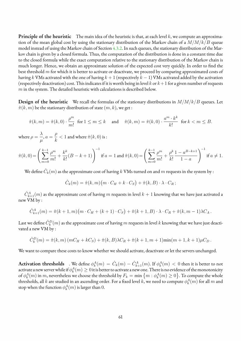
Principle of the heuristic The main idea of the heuristic is that, at each level k, we compute an approxima-tion of the mean global cost by using the stationary distribution of the Markov chain of aM/M/k/B queuemodel instead of using theMarkov chain of Section 4.3.2. In such queues, the stationary distribution of theMar-kov chain is given by a closed formula. Thus, the computation of the distribution is done in a constant time dueto the closed formula while the exact computation relative to the stationary distribution of the Markov chain ismuch longer. Hence, we obtain an approximate solution of the expected cost very quickly. In order to find thebest thresholdm for which it is better to activate or deactivate, we proceed by comparing approximated costs ofhaving k VMs activated with the one of having k + 1 (respectively k− 1) VMs activated added by the activation(respectively deactivation) cost. This indicates if it is worth being in level k or k+1 for a given number of requestsm in the system. The detailed heuristic with calculations is described below.

Design of the heuristic We recall the formulas of the stationary distributions inM/M/k/B queues. Letπ(k,m) be the stationary distribution of state (m, k), we get :

π(k,m) = π(k, 0) · ρm

m!for 1 ≤ m ≤ k and π(k,m) = π(k, 0) · a

m · kk

k!for k < m ≤ B.

where ρ =λ

µ, a =

ρ

k< 1 and where π(k, 0) is :

π(k, 0)=

(k−1∑m=0

ρm

m!+kk

k!(B − k + 1)

)−1

if a = 1 and π(k, 0)=

(k−1∑m=0

ρm

m!+ρk

k!

1− aB−k+1

1− a

)−1

if a 6= 1.

We define Ck(m) as the approximate cost of having k VMs turned on andm requests in the system by :

Ck(m) = π(k,m)(m · CH + k · CS

)+ π(k,B) · λ · CR ;

CAk+1(m) as the approximate cost of havingm requests in level k + 1 knowing that we have just activated a

new VM by :

CAk+1(m) = π(k + 1,m)

(m · CH + (k + 1) · CS

)+ π(k + 1, B) · λ · CR + π(k,m− 1)λCA .

Last we define CDk (m) as the approximate cost of havingm requests in level k knowing that we have just deacti-

vated a new VM by :

CDk (m) = π(k,m) (mCH + kCS) + π(k,B)λCR + π(k + 1,m+ 1)min(m+ 1, k + 1)µCD .

Wewant to compare these costs to know whether we should activate, deactivate or let the servers unchanged.

Activation thresholds . We define φAk (m) = Ck(m) − CAk+1(m). If φAk (m) < 0 then it is better to not

activate anew serverwhile ifφAk (m) ≥ 0 it is better to activate anewone.There is no evidenceof themonotonicityof φAk (m) inm, nevertheless we choose the threshold by Fk = min

{m : φAk (m) ≥ 0

}. To compute the whole

thresholds, all k are studied in an ascending order. For a fixed level k, we need to compute φAk (m) for allm andstop when the function φAk (m) is larger than 0.

61

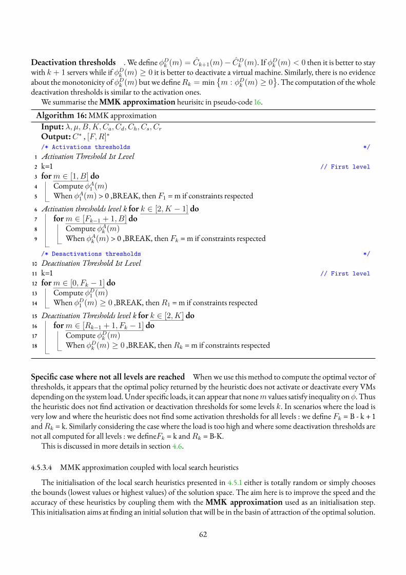
Deactivation thresholds . We define φDk (m) = Ck+1(m)− CDk (m). If φDk (m) < 0 then it is better to stay

with k + 1 servers while if φDk (m) ≥ 0 it is better to deactivate a virtual machine. Similarly, there is no evidenceabout themonotonicity ofφDk (m) but we defineRk = min

{m : φDk (m) ≥ 0

}. The computation of the whole

deactivation thresholds is similar to the activation ones.We summarise theMMK approximation heurisitc in pseudo-code 16.

Algorithm 16:MMK approximationInput: λ, µ,B,K,Ca, Cd, Ch, Cs, CrOutput:C∗ , [F,R]∗

/* Activations thresholds */1 Activation Threshold 1st Level2 k=1 // First level3 form ∈ [1, B] do4 Compute φA1 (m)5 When φA1 (m) > 0 ,BREAK, then F1 =m if constraints respected6 Activation thresholds level k for k ∈ [2, K − 1] do7 form ∈ [Fk−1 + 1, B] do8 Compute φAk (m)9 When φAk (m) > 0 ,BREAK, then Fk =m if constraints respected

/* Desactivations thresholds */10 Deactivation Threshold 1st Level11 k=1 // First level12 form ∈ [0, Fk − 1] do13 Compute φD1 (m)14 When φD1 (m) ≥ 0 ,BREAK, thenR1 =m if constraints respected15 Deactivation Thresholds level k for k ∈ [2, K] do16 form ∈ [Rk−1 + 1, Fk − 1] do17 Compute φDk (m)18 When φDk (m) ≥ 0 ,BREAK, thenRk =m if constraints respected

Specific case where not all levels are reached Whenwe use this method to compute the optimal vector ofthresholds, it appears that the optimal policy returned by the heuristic does not activate or deactivate every VMsdepending on the system load.Under specific loads, it can appear that nonem values satisfy inequality onφ. Thusthe heuristic does not find activation or deactivation thresholds for some levels k. In scenarios where the load isvery low and where the heuristic does not find some activation thresholds for all levels : we define Fk = B - k + 1andRk = k. Similarly considering the case where the load is too high and where some deactivation thresholds arenot all computed for all levels : we defineFk = k andRk = B-K.

This is discussed in more details in section 4.6.

4.5.3.4 MMK approximation coupled with local search heuristics

The initialisation of the local search heuristics presented in 4.5.1 either is totally random or simply choosesthe bounds (lowest values or highest values) of the solution space. The aim here is to improve the speed and theaccuracy of these heuristics by coupling them with the MMK approximation used as an initialisation step.This initialisation aims at finding an initial solution that will be in the basin of attraction of the optimal solution.

62

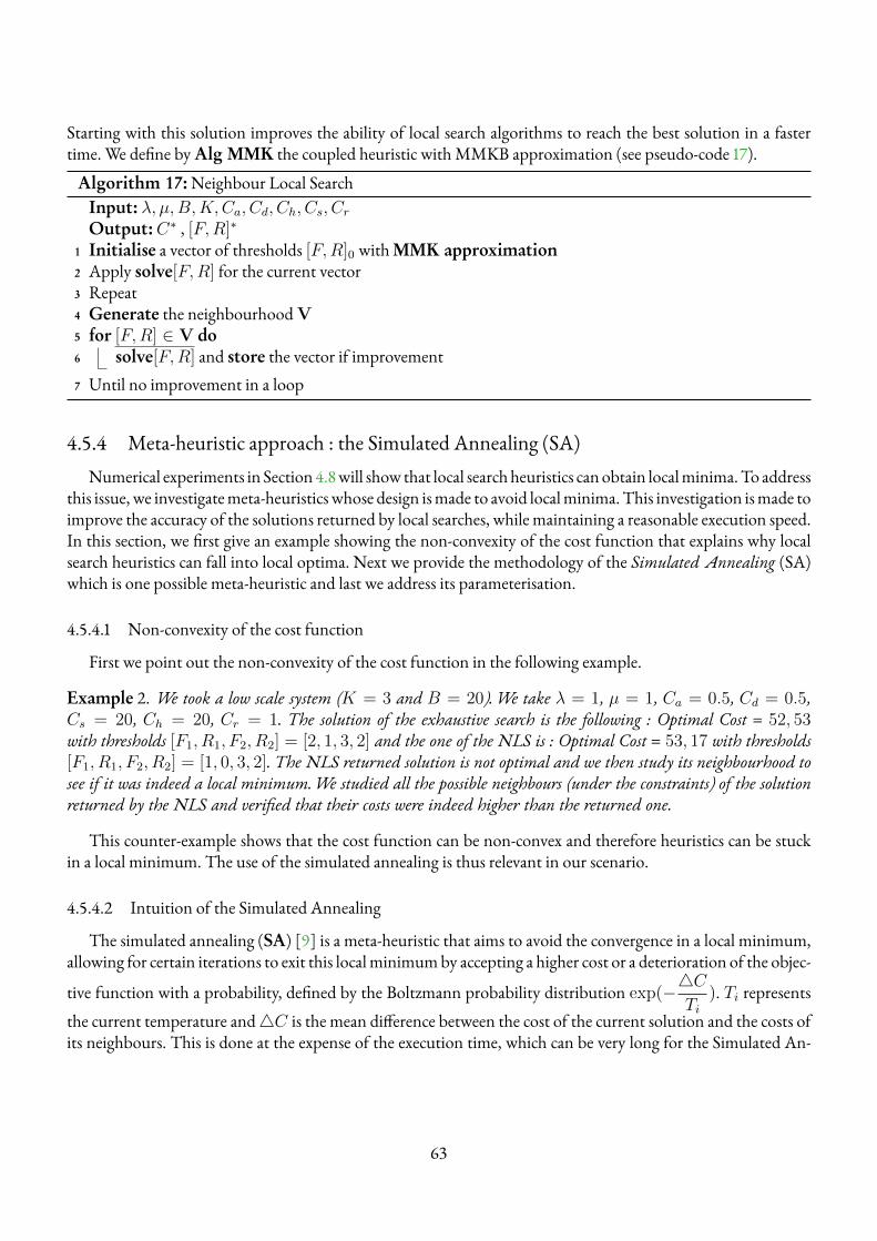
Starting with this solution improves the ability of local search algorithms to reach the best solution in a fastertime. We define by Alg MMK the coupled heuristic with MMKB approximation (see pseudo-code 17).

Algorithm 17:Neighbour Local SearchInput: λ, µ,B,K,Ca, Cd, Ch, Cs, CrOutput:C∗ , [F,R]∗

1 Initialise a vector of thresholds [F,R]0 withMMK approximation2 Apply solve[F,R] for the current vector3 Repeat4 Generate the neighbourhoodV5 for [F,R] ∈ V do6 solve[F,R] and store the vector if improvement7 Until no improvement in a loop

4.5.4 Meta-heuristic approach : the Simulated Annealing (SA)Numerical experiments in Section 4.8will show that local searchheuristics can obtain localminima.To address

this issue, we investigatemeta-heuristics whose design ismade to avoid localminima.This investigation ismade toimprove the accuracy of the solutions returned by local searches, while maintaining a reasonable execution speed.In this section, we first give an example showing the non-convexity of the cost function that explains why localsearch heuristics can fall into local optima. Next we provide the methodology of the Simulated Annealing (SA)which is one possible meta-heuristic and last we address its parameterisation.

4.5.4.1 Non-convexity of the cost function

First we point out the non-convexity of the cost function in the following example.

Example 2. We took a low scale system (K = 3 and B = 20). We take λ = 1, µ = 1, Ca = 0.5, Cd = 0.5,Cs = 20, Ch = 20, Cr = 1. The solution of the exhaustive search is the following : Optimal Cost = 52, 53with thresholds [F1, R1, F2, R2] = [2, 1, 3, 2] and the one of the NLS is : Optimal Cost = 53, 17 with thresholds[F1, R1, F2, R2] = [1, 0, 3, 2]. The NLS returned solution is not optimal and we then study its neighbourhood tosee if it was indeed a local minimum. We studied all the possible neighbours (under the constraints) of the solutionreturned by the NLS and verified that their costs were indeed higher than the returned one.

This counter-example shows that the cost function can be non-convex and therefore heuristics can be stuckin a local minimum. The use of the simulated annealing is thus relevant in our scenario.

4.5.4.2 Intuition of the Simulated Annealing

The simulated annealing (SA) [9] is a meta-heuristic that aims to avoid the convergence in a local minimum,allowing for certain iterations to exit this localminimumby accepting a higher cost or a deterioration of the objec-

tive function with a probability, defined by the Boltzmann probability distribution exp(−4CTi

). Ti representsthe current temperature and4C is the mean difference between the cost of the current solution and the costs ofits neighbours. This is done at the expense of the execution time, which can be very long for the Simulated An-

63

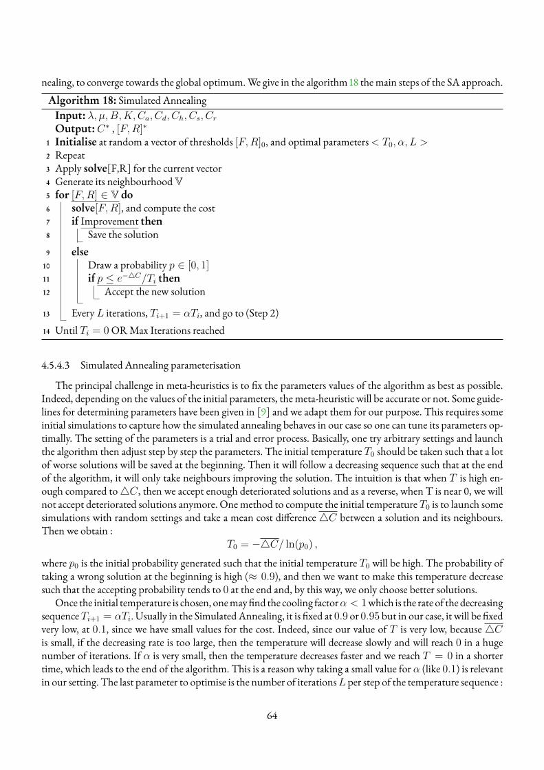
nealing, to converge towards the global optimum.We give in the algorithm 18 themain steps of the SA approach.

Algorithm 18: Simulated AnnealingInput: λ, µ,B,K,Ca, Cd, Ch, Cs, CrOutput:C∗ , [F,R]∗

1 Initialise at random a vector of thresholds [F,R]0, and optimal parameters< T0, α, L >2 Repeat3 Apply solve[F,R] for the current vector4 Generate its neighbourhoodV5 for [F,R] ∈ V do6 solve[F,R], and compute the cost7 if Improvement then8 Save the solution9 else

10 Draw a probability p ∈ [0, 1]11 if p ≤ e−4C/Ti then12 Accept the new solution

13 Every L iterations, Ti+1 = αTi, and go to (Step 2)14 Until Ti = 0 ORMax Iterations reached

4.5.4.3 Simulated Annealing parameterisation

The principal challenge in meta-heuristics is to fix the parameters values of the algorithm as best as possible.Indeed, depending on the values of the initial parameters, the meta-heuristic will be accurate or not. Some guide-lines for determining parameters have been given in [9] and we adapt them for our purpose. This requires someinitial simulations to capture how the simulated annealing behaves in our case so one can tune its parameters op-timally. The setting of the parameters is a trial and error process. Basically, one try arbitrary settings and launchthe algorithm then adjust step by step the parameters. The initial temperature T0 should be taken such that a lotof worse solutions will be saved at the beginning. Then it will follow a decreasing sequence such that at the endof the algorithm, it will only take neighbours improving the solution. The intuition is that when T is high en-ough compared to4C , then we accept enough deteriorated solutions and as a reverse, when T is near 0, we willnot accept deteriorated solutions anymore. Onemethod to compute the initial temperature T0 is to launch somesimulations with random settings and take a mean cost difference4C between a solution and its neighbours.Then we obtain :

T0 = −4C/ ln(p0) ,

where p0 is the initial probability generated such that the initial temperature T0 will be high. The probability oftaking a wrong solution at the beginning is high (≈ 0.9), and then we want to make this temperature decreasesuch that the accepting probability tends to 0 at the end and, by this way, we only choose better solutions.

Once the initial temperature is chosen, onemay find the cooling factorα < 1which is the rate of thedecreasingsequenceTi+1 = αTi. Usually in the Simulated Annealing, it is fixed at 0.9 or 0.95 but in our case, it will be fixedvery low, at 0.1, since we have small values for the cost. Indeed, since our value of T is very low, because 4Cis small, if the decreasing rate is too large, then the temperature will decrease slowly and will reach 0 in a hugenumber of iterations. If α is very small, then the temperature decreases faster and we reach T = 0 in a shortertime, which leads to the end of the algorithm. This is a reason why taking a small value for α (like 0.1) is relevantin our setting. The last parameter to optimise is the number of iterationsL per step of the temperature sequence :

64

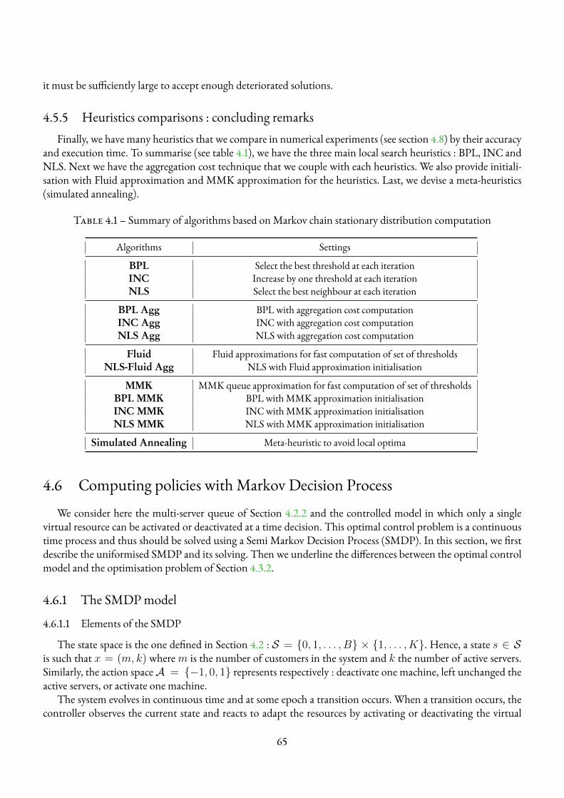
it must be sufficiently large to accept enough deteriorated solutions.

4.5.5 Heuristics comparisons : concluding remarksFinally, we have many heuristics that we compare in numerical experiments (see section 4.8) by their accuracy

and execution time. To summarise (see table 4.1), we have the three main local search heuristics : BPL, INC andNLS. Next we have the aggregation cost technique that we couple with each heuristics. We also provide initiali-sation with Fluid approximation and MMK approximation for the heuristics. Last, we devise a meta-heuristics(simulated annealing).

Table 4.1 – Summary of algorithms based onMarkov chain stationary distribution computation

Algorithms Settings

BPL Select the best threshold at each iterationINC Increase by one threshold at each iterationNLS Select the best neighbour at each iteration

BPL Agg BPL with aggregation cost computationINC Agg INC with aggregation cost computationNLS Agg NLS with aggregation cost computation

Fluid Fluid approximations for fast computation of set of thresholdsNLS-Fluid Agg NLS with Fluid approximation initialisation

MMK MMK queue approximation for fast computation of set of thresholdsBPL MMK BPL withMMK approximation initialisationINC MMK INC withMMK approximation initialisationNLS MMK NLS withMMK approximation initialisation

Simulated Annealing Meta-heuristic to avoid local optima

4.6 Computing policies with Markov Decision ProcessWe consider here the multi-server queue of Section 4.2.2 and the controlled model in which only a single

virtual resource can be activated or deactivated at a time decision. This optimal control problem is a continuoustime process and thus should be solved using a Semi Markov Decision Process (SMDP). In this section, we firstdescribe the uniformised SMDP and its solving. Then we underline the differences between the optimal controlmodel and the optimisation problem of Section 4.3.2.

4.6.1 The SMDPmodel

4.6.1.1 Elements of the SMDP

The state space is the one defined in Section 4.2 : S = {0, 1, . . . , B} × {1, . . . , K}. Hence, a state s ∈ Sis such that x = (m, k) wherem is the number of customers in the system and k the number of active servers.Similarly, the action spaceA = {−1, 0, 1} represents respectively : deactivate one machine, left unchanged theactive servers, or activate one machine.

The system evolves in continuous time and at some epoch a transition occurs. When a transition occurs, thecontroller observes the current state and reacts to adapt the resources by activating or deactivating the virtual

65

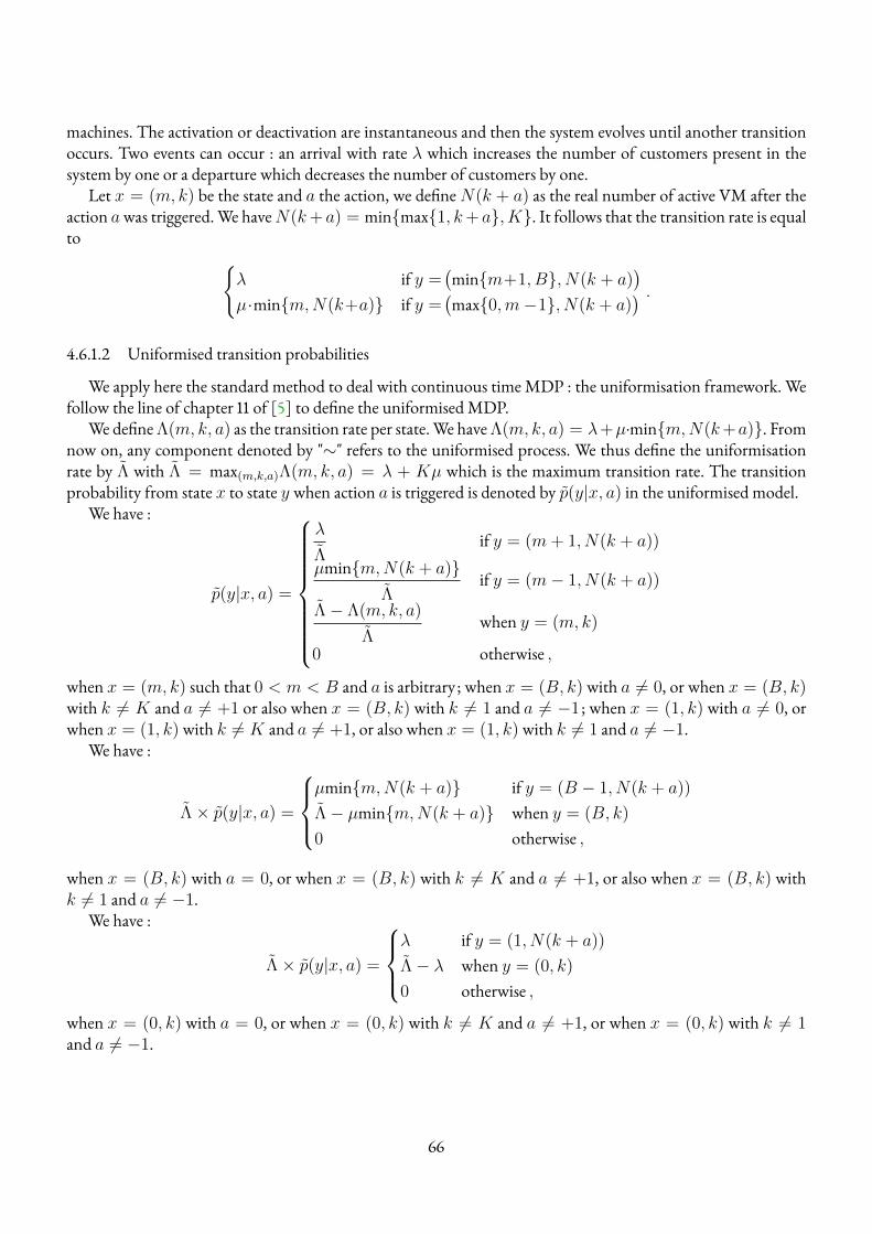
machines. The activation or deactivation are instantaneous and then the system evolves until another transitionoccurs. Two events can occur : an arrival with rate λ which increases the number of customers present in thesystem by one or a departure which decreases the number of customers by one.

Let x = (m, k) be the state and a the action, we defineN(k + a) as the real number of active VM after theaction awas triggered.We haveN(k+ a) = min{max{1, k+ a}, K}. It follows that the transition rate is equalto {

λ if y =(min{m+1, B}, N(k + a)

)µ·min{m,N(k+a)} if y =

(max{0,m−1}, N(k + a)

) .4.6.1.2 Uniformised transition probabilities

We apply here the standard method to deal with continuous timeMDP : the uniformisation framework. Wefollow the line of chapter 11 of [5] to define the uniformisedMDP.

We defineΛ(m, k, a) as the transition rate per state.We haveΛ(m, k, a) = λ+µ·min{m,N(k+a)}. Fromnow on, any component denoted by "∼" refers to the uniformised process. We thus define the uniformisationrate by Λ with Λ = max(m,k,a)Λ(m, k, a) = λ + Kµ which is the maximum transition rate. The transitionprobability from state x to state y when action a is triggered is denoted by p(y|x, a) in the uniformised model.

We have :

p(y|x, a) =

λ

Λif y = (m+ 1, N(k + a))

µmin{m,N(k + a)}Λ

if y = (m− 1, N(k + a))

Λ− Λ(m, k, a)

Λwhen y = (m, k)

0 otherwise ,

when x = (m, k) such that 0 < m < B and a is arbitrary ; when x = (B, k) with a 6= 0, or when x = (B, k)with k 6= K and a 6= +1 or also when x = (B, k) with k 6= 1 and a 6= −1 ; when x = (1, k) with a 6= 0, orwhen x = (1, k) with k 6= K and a 6= +1, or also when x = (1, k) with k 6= 1 and a 6= −1.

We have :

Λ× p(y|x, a) =

µmin{m,N(k + a)} if y = (B − 1, N(k + a))

Λ− µmin{m,N(k + a)} when y = (B, k)

0 otherwise ,

when x = (B, k) with a = 0, or when x = (B, k) with k 6= K and a 6= +1, or also when x = (B, k) withk 6= 1 and a 6= −1.

We have :

Λ× p(y|x, a) =

λ if y = (1, N(k + a))

Λ− λ when y = (0, k)

0 otherwise ,

when x = (0, k) with a = 0, or when x = (0, k) with k 6= K and a 6= +1, or when x = (0, k) with k 6= 1and a 6= −1.

66

4.6.1.3 The uniformised stage costs

We take the definition of costs of Section 4.2.2. Instantaneous costs are charged only once and are related toactivation, deactivation and losses. Accumulated costs are accumulated over time and are related to consumptionand holding cost.

k(x, a) =(CA1{a=1} + CD1{a=−1}

)+ CR.1{m=B} and r(x, a) =

(N(k + a) · CS +m · CH

).

∀x ∈ S , c(x, a) = k(x, a) + E

∫τ

0

r(x, a).dt

where τ is a r.v. following an exponential law of parameter Λ(x, a)

τ ∼ E(Λ(x, a))

So, we have :

∀x ∈ S , c(x, a) = k(x, a) +

∫∞

0

∫z

0

r(x, a).Λ(x, a). exp−Λ(x,a)z .dt.dz

∀x ∈ S , c(x, a) = k(x, a) + r(x, a).

∫∞

0

∫z

0

Λ(x, a). exp−Λ(x,a)z .dt.dz

∀x ∈ S , c(x, a) = k(x, a) + r(x, a).

∫∞

0

∫z

0

dt.Λ(x, a). exp−Λ(x,a)z .dz

∀x ∈ S , c(x, a) = k(x, a) + r(x, a).

∫∞

0

z.Λ(x, a). exp−Λ(x,a)z .dz

︸ ︷︷ ︸= 1 /Λ(x, a) because E[τ ]

Finally, we obtain [5] :

∀x ∈ S , c(x, a) = k(x, a) + r(x, a).1

Λ(x, a)(4.9)

For the treatment of stage costs, the non uniformised instantaneous costs and accumulated costs should bemultiplied by (Λ(x, a)/Λ) to get the uniformised costs.

k(x, a) =(CA1{a=1}+CD1{a=−1}

)Λ(x, a)

Λ+λ

ΛCR.1{m=B} and r(x, a) =

1

Λ

(N(k+ a) ·CS +m ·CH

).

c(x, a) = k(x, a) + r(x, a) .

67

After uniformisation of instantaneous and accumulated costs (Chapter 11.5 of [5]), we obtain the followingequation of the uniformised stage cost for x = (m, k) :

c(x, a) =(CA1{a=1} + CD1{a=−1}

)Λ(x, a)

Λ+λ

ΛCR1{m=B} +

1

Λ

(N(k + a) · CS +m · CH

).

Objective function The objective function defined in Equation (4.1) translates for all x ∈ S into

ρπ(x) = limN→∞

Eπ[ 1

N

N−1∑t=0

c(xt, π(xt)) | x0 = x],

for a given policy π. The value ρπ is the expected stage cost and equals C when actions follow policy π.

4.6.2 Solving the MDP

4.6.2.1 Classification of the SMDP

Our SMDP is an average cost model. This is why, the expected stage costs depend on the recurrent propertiesof the underlying Markov chain that is generated by a deterministic policy. A classification is then necessary tostudy them. We use the classification scheme of [5]. For communicating multichain SMDP, [67] insures thatuniformisation does not break neither structural properties of the generator nor the optimality of the policycomputed in the uniformised model.Definition 7 (Chapter 8.3.1 in [5]). AMDP is :

i Unichain if, the transitionmatrix corresponding to every deterministic stationary policy is unichain, that is,it consists of a single recurrent class, plus a possibly empty set of transient states ;

ii Multichain if, the transition matrix corresponding to at least one deterministic stationary policy containstwo or more recurrent classes ;

iii Communicating if, for every pair of state x and y inS , there exists a deterministic stationary policy π underwhich y is accessible from x, that is, pnπ(y, x) > 0 for some n ≥ 1 ;

Proposition 2. The MDP is multichain. There is a stationary deterministic policy with monotone hysteresisproperties that induces a corresponding Markov chain with more than two di�erent recurrent classes.

Proof. We assume thatK ≥ 2 and let k be such that k ∈ [1, . . . , K]. We define the policy q as follows. Forany level l such that l < k − 1, we have only activation. This means that there existsm ∈ [0, · · · , B] such thatq(m′, l) = 1 for anym ≤ m′ and q(m, l) ≤ q(m, l− 1). For level k we have neither activation nor deactivationand q(m, k) = 0 for allm ∈ [0, · · · , B]. For any level l with l > k + 1, we have only deactivation. There existsm ∈ [0, · · · , B] such that q(m′, l) = −1 for anym′ ≤ m and q(m, l) ≥ q(m, l + 1).

Hence, starting from any state such that l < k− 1, then the highest attainable level is k− 1. Equally, startingfrom any state of the level k, we remain in this level. At last, starting from any state such that l ≥ k+ 1, then thelowest attainable level is k+ 1. Therefore, we have three recurrent classes : the level k, the level k− 1 and the levelk + 1 (and two recurrent classes forK = 2).�

We display an example in Figure 4.8 of an isotone hysteresis multichain MDP.

Lemma 3. The MDP is communicating. There exists a stationary isotone hysteresis policy such that the correspon-ding Markov chain is irreducible.

68

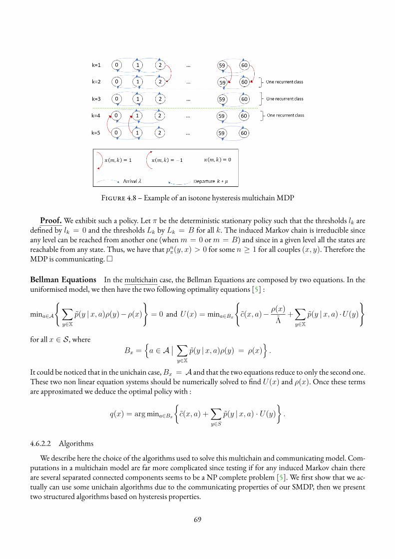
Figure 4.8 – Example of an isotone hysteresis multichain MDP

Proof. We exhibit such a policy. Let π be the deterministic stationary policy such that the thresholds lk aredefined by lk = 0 and the thresholds Lk by Lk = B for all k. The induced Markov chain is irreducible sinceany level can be reached from another one (whenm = 0 orm = B) and since in a given level all the states arereachable from any state. Thus, we have that pnπ(y, x) > 0 for some n ≥ 1 for all couples (x, y). Therefore theMDP is communicating.�

Bellman Equations In the multichain case, the Bellman Equations are composed by two equations. In theuniformised model, we then have the two following optimality equations [5] :

mina∈A

{∑y∈X

p(y |x, a)ρ(y)−ρ(x)

}= 0 and U(x) = mina∈Bx

{c(x, a)− ρ(x)

Λ+∑y∈X

p(y |x, a) ·U(y)

}

for all x ∈ S , whereBx =

{a ∈ A

∣∣ ∑y∈X

p(y |x, a)ρ(y) = ρ(x)}.

It could be noticed that in the unichain case,Bx = A and that the two equations reduce to only the second one.These two non linear equation systems should be numerically solved to find U(x) and ρ(x). Once these termsare approximated we deduce the optimal policy with :

q(x) = argmina∈Bx

{c(x, a) +

∑y∈S

p(y |x, a) · U(y)

}.

4.6.2.2 Algorithms

We describe here the choice of the algorithms used to solve this multichain and communicating model. Com-putations in a multichain model are far more complicated since testing if for any induced Markov chain thereare several separated connected components seems to be a NP complete problem [5]. We first show that we ac-tually can use some unichain algorithms due to the communicating properties of our SMDP, then we presenttwo structured algorithms based on hysteresis properties.

69

Unichain algorithms From[5] it exists amultichainpolicy iteration algorithm that solvesmultichainmodels.It requires to solve two equation systems and thus is time consuming. However, by Proposition 3, our MDP iscommunicating and in Theorem 8.3.2 of [5] it is proved that unichain value iteration algorithm converges to theoptimal value in communicating models. This property allows us to use the unichain value iteration algorithm.

There is also, in [5], a policy iteration algorithm for communicating models. It requires to start with an initialunichain policy and its inner loop roughly differs from the unichain case in order to keep some properties. Wedecide to use here algorithms based on unichain policy iteration. There does not exist theoretical guarantee oftheir convergence, but we showed in numerical experiments that they always converge to the same policy thanvalue iteration.

Four different usual unichain algorithms will be considered : Value Iteration, Relative value iteration, PolicyIteration modified and Policy Iteration modified adapted, which adapts its precision during the policy evaluationstep. They are respectively referred by VI, RVI, PI and PI Adapt. The algorithms are all described in [5] and arealready implemented in the software [66].

Structured Policies algorithm We now integrate hysteresis properties in the algorithms. Two classes of po-licies have been investigated : Double Level class (Definition 2) and Monotone Hysteresis class (Definition 5).The goal is to plug hysteresis assumptions during the policy improvement step of policy iteration. This allows totest less actions at each iteration and to speed up the algorithm. Two algorithms are implemented : one for thedouble level properties (referred asDL-PI ) and one for the hysteresis properties (referred asHy-PI ). We describein pseudocodes 19 and 20 the modified policy iteration algorithms with integration of structural properties.

The properties of Double Level and Hysteresis policies induce some constraints on the best action selectionin the Policy improvement step, mainly by restricting the choice of possible actions :∗ Double Level : FromDefinition 2, the rule (policy) q(m, k) is increasing in the number of jobs in the systemm. This increasing property is integrated such that when we choose the best action, the set of decision isconstrained. As an example : suppose that q(0, k) = 0, then q(1, k) ≥ 0 which impose to test only twoactions over three.∗ Hysteresis : The hysteresis property integrates the Double Level property plus a supplementary constrainton the number of activated resources k. Indeed the hysteresis property, for a single activation setting, insuresthat q(., k) is decreasing in k. As an example : suppose that q(m, 1) = 0, then q(m, 2) ≤ 0 which imposeto test only two actions over three.

To integrate these properties, the policy improvement step is modified. We divide the process by the dimen-sions of the state (m, k). We first fix the level k and take the best actions for allm in an increasing order such thatwe consider the increasing property of q inm. For the hysteresis constraint, when we move from level k to level

70

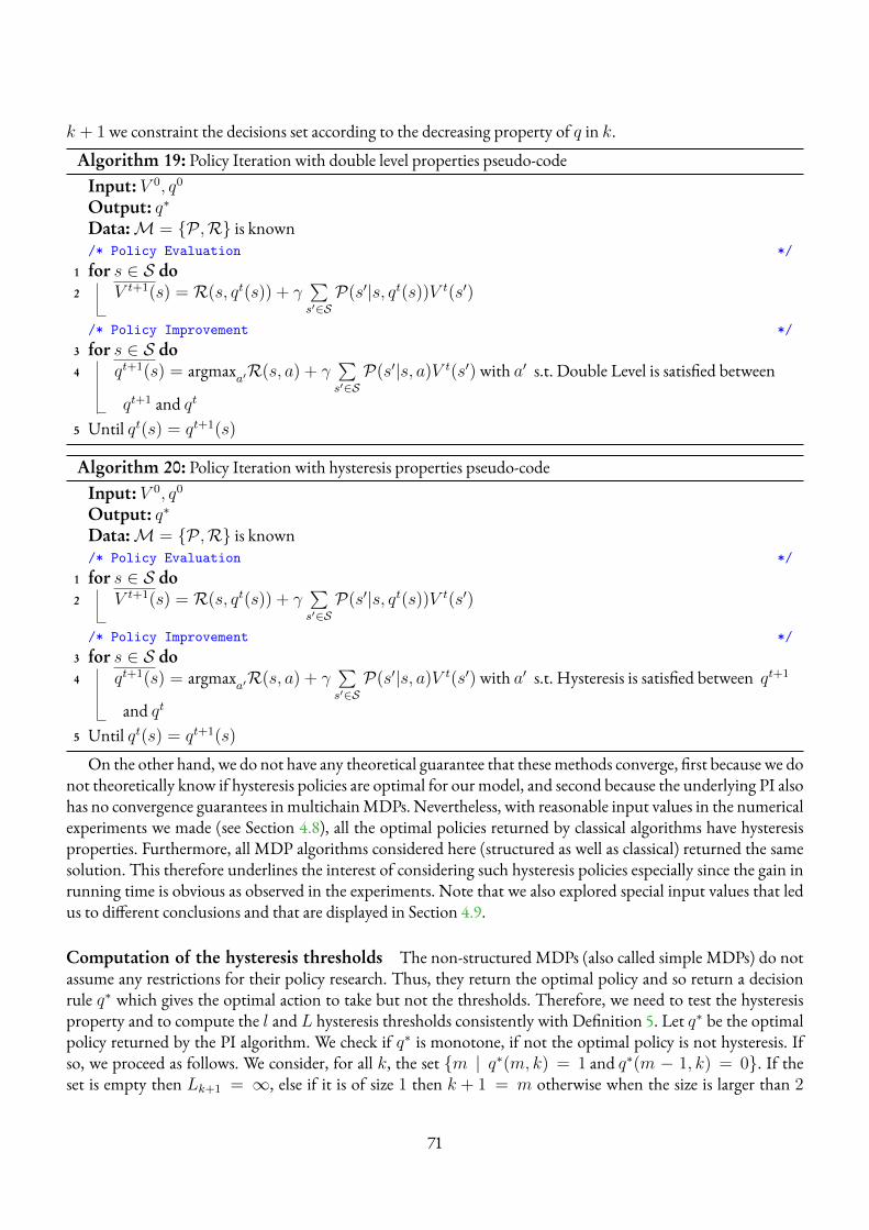
k + 1 we constraint the decisions set according to the decreasing property of q in k.

Algorithm 19: Policy Iteration with double level properties pseudo-codeInput: V 0, q0

Output: q∗

Data:M = {P ,R} is known/* Policy Evaluation */

1 for s ∈ S do2 V t+1(s) = R(s, qt(s)) + γ

∑s′∈SP(s′|s, qt(s))V t(s′)

/* Policy Improvement */3 for s ∈ S do4 qt+1(s) = argmaxa′R(s, a) + γ

∑s′∈SP(s′|s, a)V t(s′) with a′ s.t. Double Level is satisfied between

qt+1 and qt

5 Until qt(s) = qt+1(s)

Algorithm 20: Policy Iteration with hysteresis properties pseudo-codeInput: V 0, q0

Output: q∗

Data:M = {P ,R} is known/* Policy Evaluation */

1 for s ∈ S do2 V t+1(s) = R(s, qt(s)) + γ

∑s′∈SP(s′|s, qt(s))V t(s′)

/* Policy Improvement */3 for s ∈ S do4 qt+1(s) = argmaxa′R(s, a) + γ

∑s′∈SP(s′|s, a)V t(s′) with a′ s.t. Hysteresis is satisfied between qt+1

and qt

5 Until qt(s) = qt+1(s)

On the other hand, we do not have any theoretical guarantee that these methods converge, first because we donot theoretically know if hysteresis policies are optimal for our model, and second because the underlying PI alsohas no convergence guarantees in multichainMDPs. Nevertheless, with reasonable input values in the numericalexperiments we made (see Section 4.8), all the optimal policies returned by classical algorithms have hysteresisproperties. Furthermore, all MDP algorithms considered here (structured as well as classical) returned the samesolution. This therefore underlines the interest of considering such hysteresis policies especially since the gain inrunning time is obvious as observed in the experiments. Note that we also explored special input values that ledus to different conclusions and that are displayed in Section 4.9.

Computation of the hysteresis thresholds The non-structured MDPs (also called simple MDPs) do notassume any restrictions for their policy research. Thus, they return the optimal policy and so return a decisionrule q∗ which gives the optimal action to take but not the thresholds. Therefore, we need to test the hysteresisproperty and to compute the l and L hysteresis thresholds consistently with Definition 5. Let q∗ be the optimalpolicy returned by the PI algorithm. We check if q∗ is monotone, if not the optimal policy is not hysteresis. Ifso, we proceed as follows. We consider, for all k, the set {m | q∗(m, k) = 1 and q∗(m − 1, k) = 0}. If theset is empty then Lk+1 = ∞, else if it is of size 1 then k + 1 = m otherwise when the size is larger than 2

71

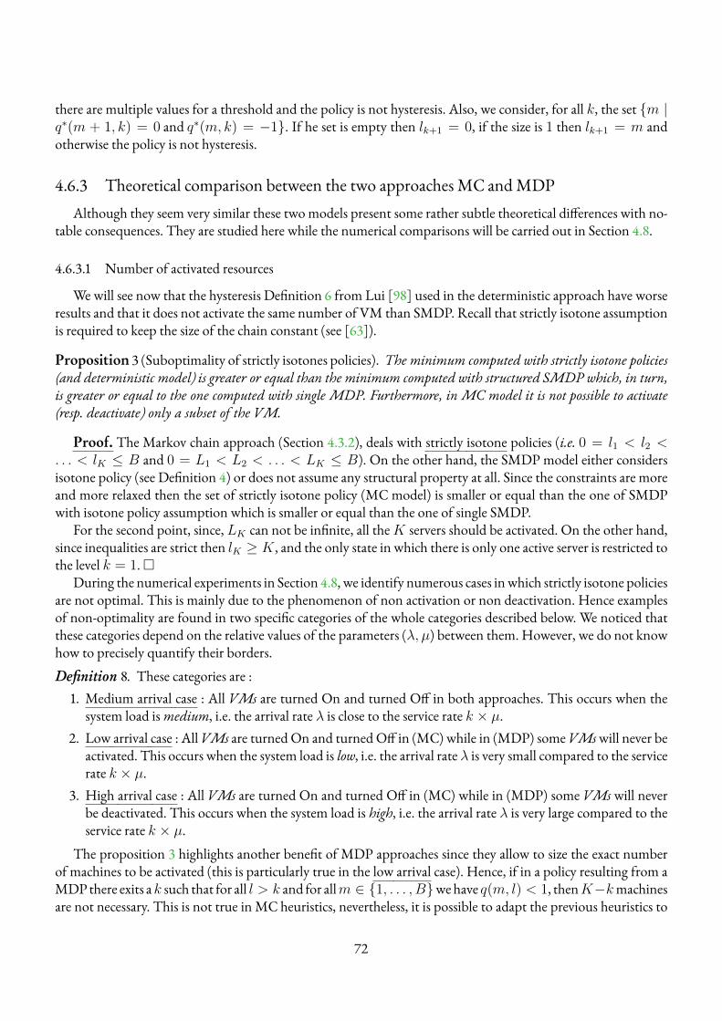
there are multiple values for a threshold and the policy is not hysteresis. Also, we consider, for all k, the set {m |q∗(m + 1, k) = 0 and q∗(m, k) = −1}. If he set is empty then lk+1 = 0, if the size is 1 then lk+1 = m andotherwise the policy is not hysteresis.

4.6.3 Theoretical comparison between the two approaches MC andMDPAlthough they seem very similar these two models present some rather subtle theoretical differences with no-

table consequences. They are studied here while the numerical comparisons will be carried out in Section 4.8.

4.6.3.1 Number of activated resources

We will see now that the hysteresis Definition 6 from Lui [98] used in the deterministic approach have worseresults and that it does not activate the same number of VM than SMDP. Recall that strictly isotone assumptionis required to keep the size of the chain constant (see [63]).

Proposition 3 (Suboptimality of strictly isotones policies). The minimum computed with strictly isotone policies(and deterministic model) is greater or equal than the minimum computed with structured SMDP which, in turn,is greater or equal to the one computed with single MDP. Furthermore, in MC model it is not possible to activate(resp. deactivate) only a subset of the VM.

Proof. The Markov chain approach (Section 4.3.2), deals with strictly isotone policies (i.e. 0 = l1 < l2 <. . . < lK ≤ B and 0 = L1 < L2 < . . . < LK ≤ B). On the other hand, the SMDP model either considersisotone policy (see Definition 4) or does not assume any structural property at all. Since the constraints are moreand more relaxed then the set of strictly isotone policy (MC model) is smaller or equal than the one of SMDPwith isotone policy assumption which is smaller or equal than the one of single SMDP.

For the second point, since, LK can not be infinite, all theK servers should be activated. On the other hand,since inequalities are strict then lK ≥ K , and the only state in which there is only one active server is restricted tothe level k = 1.�

During the numerical experiments in Section 4.8, we identify numerous cases inwhich strictly isotone policiesare not optimal. This is mainly due to the phenomenon of non activation or non deactivation. Hence examplesof non-optimality are found in two specific categories of the whole categories described below. We noticed thatthese categories depend on the relative values of the parameters (λ, µ) between them. However, we do not knowhow to precisely quantify their borders.Definition 8. These categories are :

1. Medium arrival case : All VMs are turned On and turned Off in both approaches. This occurs when thesystem load ismedium, i.e. the arrival rate λ is close to the service rate k × µ.

2. Low arrival case : AllVMs are turned On and turned Off in (MC) while in (MDP) someVMswill never beactivated. This occurs when the system load is low, i.e. the arrival rate λ is very small compared to the servicerate k × µ.

3. High arrival case : All VMs are turned On and turned Off in (MC) while in (MDP) some VMs will neverbe deactivated. This occurs when the system load is high, i.e. the arrival rate λ is very large compared to theservice rate k × µ.

The proposition 3 highlights another benefit of MDP approaches since they allow to size the exact numberof machines to be activated (this is particularly true in the low arrival case). Hence, if in a policy resulting from aMDPthere exits ak such that for all l > k and for allm ∈ {1, . . . , B}wehave q(m, l) < 1, thenK−kmachinesare not necessary. This is not true in MC heuristics, nevertheless, it is possible to adapt the previous heuristics to

72

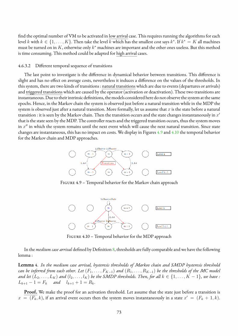
find the optimal number of VM to be activated in low arrival case. This requires running the algorithms for eachlevel k with k ∈ {1, . . . , K}. Then take the level k which has the smallest cost says k∗. If k∗ = K all machinesmust be turned on inK , otherwise only k∗ machines are important and the other ones useless. But this methodis time consuming. This method could be adapted for high arrival cases.

4.6.3.2 Different temporal sequence of transitions

The last point to investigate is the difference in dynamical behavior between transitions. This difference isslight and has no effect on average costs, nevertheless it induces a difference on the values of the thresholds. Inthis system, there are two kinds of transitions : natural transitions which are due to events (departures or arrivals)and triggered transitions which are caused by the operator (activation or deactivation). These two transitions areinstantaneous.Due to their intrinsic definitions, themodels consideredhere donot observe the systemat the sameepochs. Hence, in theMarkov chain the system is observed just before a natural transition while in theMDP thesystem is observed just after a natural transition. More formally, let us assume that x is the state before a naturaltransition : it is seen by theMarkov chain. Then the transition occurs and the state changes instantaneously in x′that is the state seen by theMDP. The controller reacts and the triggered transition occurs, thus the systemmovesin x′′ in which the system remains until the next event which will cause the next natural transition. Since statechanges are instantaneous, this has no impact on costs. We display in Figures 4.9 and 4.10 the temporal behaviorfor the Markov chain andMDP approaches.

Figure 4.9 – Temporal behavior for the Markov chain approach

Figure 4.10 – Temporal behavior for the MDP approach

In themedium case arrival defined byDefinition 8, thresholds are fully comparable andwe have the followinglemma :

Lemma 4. In the medium case arrival, hysteresis thresholds of Markov chain and SMDP hysteresis thresholdcan be inferred from each other. Let (F1, . . . , FK−1) and (R1, . . . , RK−1) be the thresholds of the MC modeland let (L2, . . . , LK) and (l2, . . . , lK) be the SMDP thresholds. Then, for all k ∈ {1, . . . , K − 1}, we have :Lk+1 − 1 = Fk and lk+1 + 1 = Rk.

Proof. We make the proof for an activation threshold. Let assume that the state just before a transition isx = (Fk, k), if an arrival event occurs then the system moves instantaneously in a state x′ = (Fk + 1, k).

73

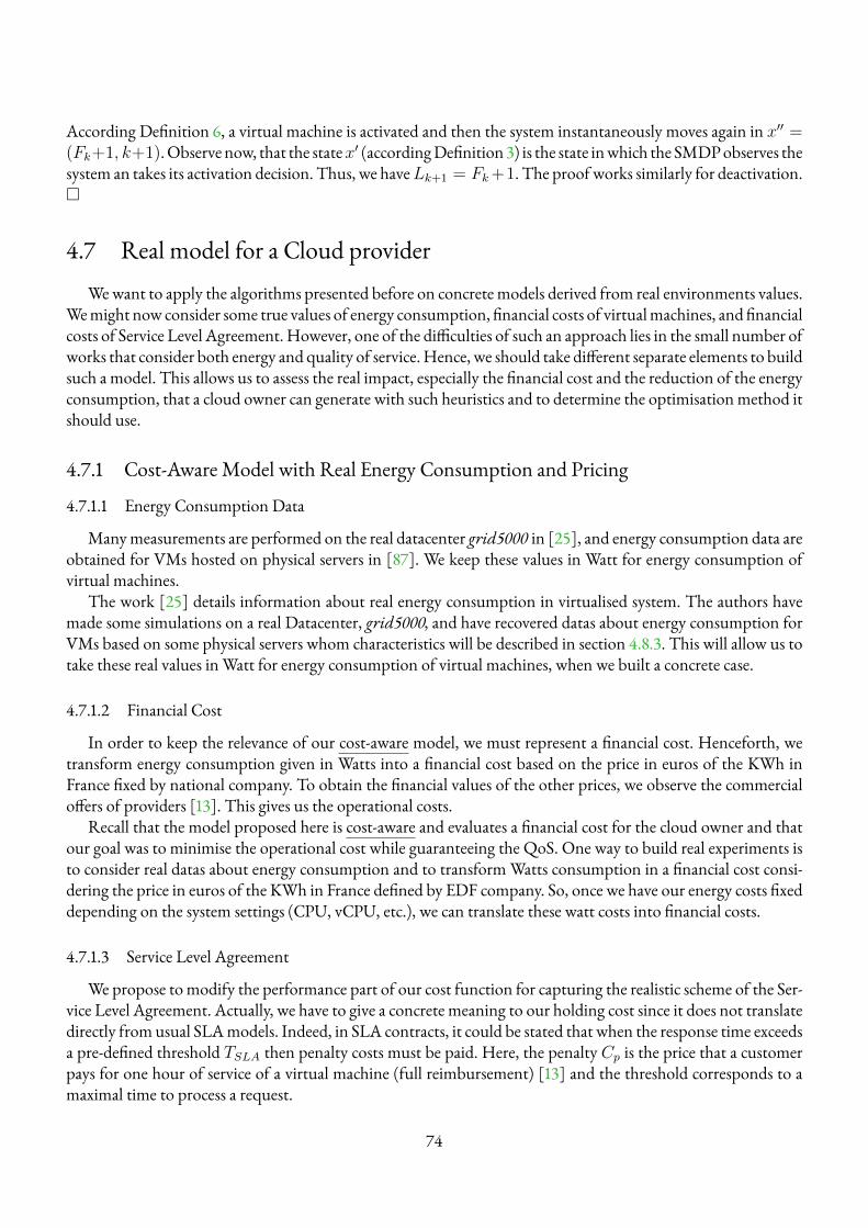
According Definition 6, a virtual machine is activated and then the system instantaneously moves again in x′′ =(Fk+1, k+1).Observe now, that the statex′ (accordingDefinition 3) is the state inwhich the SMDPobserves thesystem an takes its activation decision. Thus, we haveLk+1 = Fk+1. The proof works similarly for deactivation.�

4.7 Real model for a Cloud providerWewant to apply the algorithms presented before on concrete models derived from real environments values.

Wemight now consider some true values of energy consumption, financial costs of virtualmachines, and financialcosts of Service Level Agreement. However, one of the difficulties of such an approach lies in the small number ofworks that consider both energy and quality of service.Hence, we should take different separate elements to buildsuch a model. This allows us to assess the real impact, especially the financial cost and the reduction of the energyconsumption, that a cloud owner can generate with such heuristics and to determine the optimisation method itshould use.

4.7.1 Cost-Aware Model with Real Energy Consumption and Pricing

4.7.1.1 Energy Consumption Data

Manymeasurements are performed on the real datacenter grid5000 in [25], and energy consumption data areobtained for VMs hosted on physical servers in [87]. We keep these values in Watt for energy consumption ofvirtual machines.

The work [25] details information about real energy consumption in virtualised system. The authors havemade some simulations on a real Datacenter, grid5000, and have recovered datas about energy consumption forVMs based on some physical servers whom characteristics will be described in section 4.8.3. This will allow us totake these real values in Watt for energy consumption of virtual machines, when we built a concrete case.

4.7.1.2 Financial Cost

In order to keep the relevance of our cost-aware model, we must represent a financial cost. Henceforth, wetransform energy consumption given in Watts into a financial cost based on the price in euros of the KWh inFrance fixed by national company. To obtain the financial values of the other prices, we observe the commercialoffers of providers [13]. This gives us the operational costs.

Recall that the model proposed here is cost-aware and evaluates a financial cost for the cloud owner and thatour goal was to minimise the operational cost while guaranteeing the QoS. One way to build real experiments isto consider real datas about energy consumption and to transformWatts consumption in a financial cost consi-dering the price in euros of the KWh in France defined by EDF company. So, once we have our energy costs fixeddepending on the system settings (CPU, vCPU, etc.), we can translate these watt costs into financial costs.

4.7.1.3 Service Level Agreement

We propose to modify the performance part of our cost function for capturing the realistic scheme of the Ser-vice Level Agreement. Actually, we have to give a concrete meaning to our holding cost since it does not translatedirectly from usual SLAmodels. Indeed, in SLA contracts, it could be stated that when the response time exceedsa pre-defined threshold TSLA then penalty costs must be paid. Here, the penalty Cp is the price that a customerpays for one hour of service of a virtual machine (full reimbursement) [13] and the threshold corresponds to amaximal time to process a request.

74

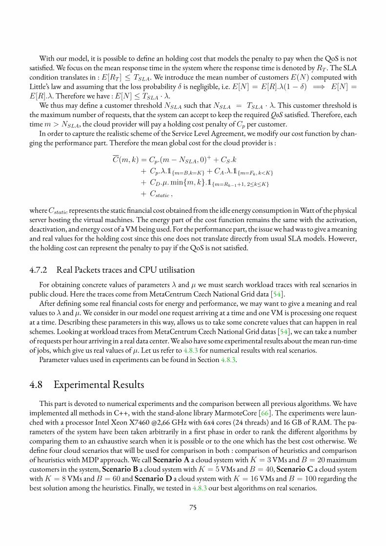
With our model, it is possible to define an holding cost that models the penalty to pay when the QoS is notsatisfied. We focus on the mean response time in the system where the response time is denoted byRT . The SLAcondition translates in : E[RT ] ≤ TSLA. We introduce the mean number of customers E(N) computed withLittle’s law and assuming that the loss probability δ is negligible, i.e. E[N ] = E[R].λ(1 − δ) =⇒ E[N ] =E[R].λ. Therefore we have :E[N ] ≤ TSLA · λ.

We thus may define a customer threshold NSLA such that NSLA = TSLA · λ. This customer threshold isthe maximum number of requests, that the system can accept to keep the requiredQoS satisfied. Therefore, eachtimem > NSLA, the cloud provider will pay a holding cost penalty ofCp per customer.

In order to capture the realistic scheme of the Service Level Agreement, wemodify our cost function by chan-ging the performance part. Therefore the mean global cost for the cloud provider is :

C(m, k) = Cp.(m−NSLA, 0)+ + CS.k

+ Cp.λ.1{m=B,k=K} + CA.λ.1{m=Fk, k<K}

+ CD.µ.min{m, k}.1{m=Rk−1+1, 2≤k≤K}

+ Cstatic ,

whereCstatic represents the static financial cost obtained from the idle energy consumption inWatt of thephysicalserver hosting the virtual machines. The energy part of the cost function remains the same with the activation,deactivation, and energy cost of aVMbeingused. For theperformancepart, the issuewehadwas to give ameaningand real values for the holding cost since this one does not translate directly from usual SLA models. However,the holding cost can represent the penalty to pay if the QoS is not satisfied.

4.7.2 Real Packets traces and CPU utilisationFor obtaining concrete values of parameters λ and µ we must search workload traces with real scenarios in

public cloud. Here the traces come fromMetaCentrum Czech National Grid data [54].After defining some real financial costs for energy and performance, we may want to give a meaning and real

values to λ and µ. We consider in our model one request arriving at a time and one VM is processing one requestat a time. Describing these parameters in this way, allows us to take some concrete values that can happen in realschemes. Looking at workload traces fromMetaCentrumCzech National Grid datas [54], we can take a numberof requests per hour arriving in a real data center.We also have some experimental results about themean run-timeof jobs, which give us real values of µ. Let us refer to 4.8.3 for numerical results with real scenarios.

Parameter values used in experiments can be found in Section 4.8.3.

4.8 Experimental ResultsThis part is devoted to numerical experiments and the comparison between all previous algorithms. We have

implemented all methods in C++, with the stand-alone library MarmoteCore [66]. The experiments were laun-ched with a processor Intel Xeon X7460 @2,66 GHz with 6x4 cores (24 threads) and 16 GB of RAM. The pa-rameters of the system have been taken arbitrarily in a first phase in order to rank the different algorithms bycomparing them to an exhaustive search when it is possible or to the one which has the best cost otherwise. Wedefine four cloud scenarios that will be used for comparison in both : comparison of heuristics and comparisonof heuristics withMDP approach.We call Scenario A a cloud systemwithK = 3VMs andB = 20maximumcustomers in the system, Scenario B a cloud systemwithK = 5VMs andB = 40, Scenario C a cloud systemwithK = 8 VMs andB = 60 and Scenario D a cloud system withK = 16 VMs andB = 100 regarding thebest solution among the heuristics. Finally, we tested in 4.8.3 our best algorithms on real scenarios.

75

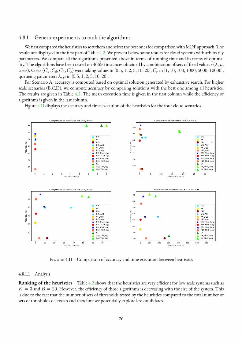
4.8.1 Generic experiments to rank the algorithmsWefirst compared theheuristics to sort themand select thebest ones for comparisonwithMDPapproach.The

results are displayed in the first part of Table 4.2.We present below some results for cloud systems with arbitrarilyparameters. We compare all the algorithms presented above in terms of running time and in terms of optima-lity. The algorithms have been tested on 46656 instances obtained by combination of sets of fixed values : (λ, µ,costs). Costs (Ca, Cd, Ch, Cs) were taking values in [0.5, 1, 2, 5, 10, 20], Cr in [1, 10, 100, 1000, 5000, 10000],queueing parameters λ, µ in [0.5, 1, 2, 5, 10, 20].

For Scenario A, accuracy is computed based on optimal solution generated by exhaustive search. For higherscale scenarios (B,C,D), we compute accuracy by comparing solutions with the best one among all heuristics.The results are given in Table 4.2. The mean execution time is given in the first column while the efficiency ofalgorithms is given in the last column.

Figure 4.11 displays the accuracy and time execution of the heuristics for the four cloud scenarios.

Figure 4.11 – Comparison of accuracy and time execution between heuristics

4.8.1.1 Analysis

Ranking of the heuristics Table 4.2 shows that the heuristics are very efficient for low scale systems such asK = 3 andB = 20. However, the efficiency of those algorithms is decreasing with the size of the system. Thisis due to the fact that the number of sets of thresholds tested by the heuristics compared to the total number ofsets of thresholds decreases and therefore we potentially explore less candidates.

76

Looking at the results of the experiment, we detect thatBPL Agg has the best percentage of optimality evenfor large systems. Unfortunately its running time is the highest. The fastest one, INC Agg returns the solutionin less than a second but reveals an accuracy which is not the worse without being impressive. At lastNLS-FluidAgg presents a good compromise keeping a good precision and returning the solution in a short time.

Aggregation method strongly improves algorithms Table 4.2 show a significant time saving offered bythe aggregation method for the same efficiency. In all cases, the aggregation method significantly improves ourheuristics and the running times of all the algorithms are widely reduced. The improvement for three virtualmachines is small, as expected, but the gain increases as the size of the system increases. Hence the running timeis divided by about 1.3 whenK = 3 and B = 20 and by about 3.8 whenK = 16 and B = 100 (e.g. BPLalgorithm passes from 757 seconds to 186 seconds).

Impact of the M/M/k approximation Coupled with heuristics BPL and NLS,M/M/k approximationbrings significant improvement considering the efficiency and the time execution. For a large scale case (ScenarioD inTable 4.2), theBPLMMKAgg provides the best solution for 87.24%of the instances in 31.7 seconds,whichis the best heuristic in terms of time-accuracy ratio. We can notice, in all cases, that coupled heuristic always havebetter accuracy than the heuristic alone. Moreover, the initialisation technique does not only improve efficiencybut also time execution. For example in Scenario C, BPL Agg has a mean time of 10,27 seconds for 79,57 %accuracy while BPL-MMk Agg obtains 95,39 % accuracy in 5,16 seconds, providing a double major gain.

Simulated annealing is not worth it We noticed that the simulated annealing suffers from a temporalovercost whatever the size of the system. Unfortunately this overcost does not allow to obtain a greater precision,since it obtains similar accuracy than some heuristics. Actually, it seems that greater precision could be obtainedat the price of a very large running time.

4.8.2 Heuristics vs MDPWe compare next the best heuristics according to section 4.8.1 with the MDP algorithms. Numerical experi-

ments have been done for the same Cloud model parameters and same system parameters. Results are displayedin Table 4.2. We first compare all the local search heuristics and their improvement inMC Heuristics. Then wecompare all the (MDP) algorithms with the value iteration solution (convergence is known from Section 4.6.2.2)inMDP, before comparison with the heuristics to compare both approaches inComparison. Again, we compareall methods for the four cloud scenarios A, B, C and D. For the heuristics, values in blue correspond to the mini-mum execution time for a given Scenario, values in red correspond to the best efficiency and values in green theones that have the best ratio optimality-time. For the comparison between MDP and Heuristics, we only pointout in green the methods with the best ratio.

4.8.2.1 Analysis

By Section 4.6.2.2, we theoretically know that value iteration algorithm converges to the exact solution. The-refore, we can use it as a benchmark to compare theMDP algorithms. Recall that we had no guarantee for conver-gence of unichain policy iteration algorithm. Yet, we observe in these numerical experiments, that all MDP algo-rithms obtain 100% of accuracy (optimal solution being given by value iteration) in all scenarios. Thus, all MDPalgorithms converge to the optimal solution. Concerning the running time, we observe that policy iteration algo-rithms PI and PI Adapted are twice as good than value iteration on all studied scenarios. Furthermore, we seethat the execution time of the structured MDP algorithms DL-PI and Hy-PI is divided by 2 compared to PI

77

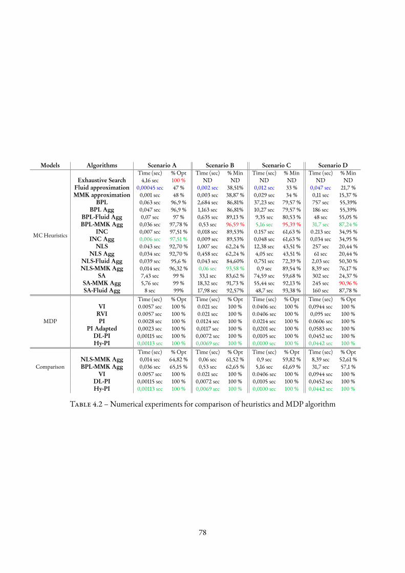
Models Algorithms Scenario A Scenario B Scenario C Scenario DTime (sec) % Opt Time (sec) %Min Time (sec) %Min Time (sec) %Min

MCHeuristics

Exhaustive Search 4,16 sec 100 % ND ND ND ND ND NDFluid approximation 0,00045 sec 47 % 0,002 sec 38,51% 0,012 sec 33 % 0,047 sec 21,7 %MMK approximation 0,001 sec 48 % 0,003 sec 38,87 % 0,029 sec 34 % 0,11 sec 15,37 %

BPL 0,063 sec 96,9 % 2,684 sec 86,81% 37,23 sec 79,57 % 757 sec 55,39%BPL Agg 0,047 sec 96,9 % 1,163 sec 86,81% 10,27 sec 79,57 % 186 sec 55,39%

BPL-Fluid Agg 0,07 sec 97 % 0,635 sec 89,13 % 9,35 sec 80,53 % 48 sec 55,05 %BPL-MMK Agg 0,036 sec 97,78 % 0,53 sec 96,59 % 5,16 sec 95,39 % 31,7 sec 87,24 %

INC 0,007 sec 97,51 % 0,018 sec 89,53% 0.157 sec 61,63 % 0.213 sec 34,95 %INC Agg 0,006 sec 97,51 % 0,009 sec 89,53% 0,048 sec 61,63 % 0,034 sec 34,95 %

NLS 0.043 sec 92,70 % 1,007 sec 62,24 % 12,38 sec 43,51 % 257 sec 20,44 %NLS Agg 0,034 sec 92,70 % 0,458 sec 62,24 % 4,05 sec 43,51 % 61 sec 20,44 %

NLS-Fluid Agg 0,039 sec 95,6 % 0,043 sec 84,60% 0,751 sec 72,39 % 2,03 sec 50,30 %NLS-MMK Agg 0,014 sec 96,32 % 0,06 sec 93,58 % 0,9 sec 89,54 % 8,39 sec 76,17 %

SA 7,43 sec 99 % 33,1 sec 83,62 % 74,59 sec 59,68 % 302 sec 24,37 %SA-MMK Agg 5,76 sec 99 % 18,32 sec 91,73 % 55,44 sec 92,13 % 245 sec 90,96 %SA-Fluid Agg 8 sec 99% 17,98 sec 92,57% 48,7 sec 93,38 % 160 sec 87,78 %

MDP

Time (sec) % Opt Time (sec) % Opt Time (sec) % Opt Time (sec) % OptVI 0.0057 sec 100 % 0.021 sec 100 % 0.0406 sec 100 % 0,0944 sec 100 %

RVI 0.0057 sec 100 % 0.021 sec 100 % 0.0406 sec 100 % 0,095 sec 100 %PI 0.0028 sec 100 % 0.0124 sec 100 % 0.0214 sec 100 % 0.0606 sec 100 %

PI Adapted 0,0023 sec 100 % 0,0117 sec 100 % 0,0201 sec 100 % 0,0583 sec 100 %DL-PI 0,00115 sec 100 % 0,0072 sec 100 % 0,0105 sec 100 % 0,0452 sec 100 %Hy-PI 0,00113 sec 100 % 0,0069 sec 100 % 0,0100 sec 100 % 0,0442 sec 100 %

Comparison

Time (sec) % Opt Time (sec) % Opt Time (sec) % Opt Time (sec) % OptNLS-MMK Agg 0,014 sec 64,82 % 0,06 sec 61,52 % 0,9 sec 59,82 % 8,39 sec 52,61 %BPL-MMK Agg 0,036 sec 65,15 % 0,53 sec 62,65 % 5,16 sec 61,69 % 31,7 sec 57,1 %

VI 0.0057 sec 100 % 0.021 sec 100 % 0.0406 sec 100 % 0,0944 sec 100 %DL-PI 0,00115 sec 100 % 0,0072 sec 100 % 0,0105 sec 100 % 0,0452 sec 100 %Hy-PI 0,00113 sec 100 % 0,0069 sec 100 % 0,0100 sec 100 % 0,0442 sec 100 %

Table 4.2 – Numerical experiments for comparison of heuristics andMDP algorithm

78

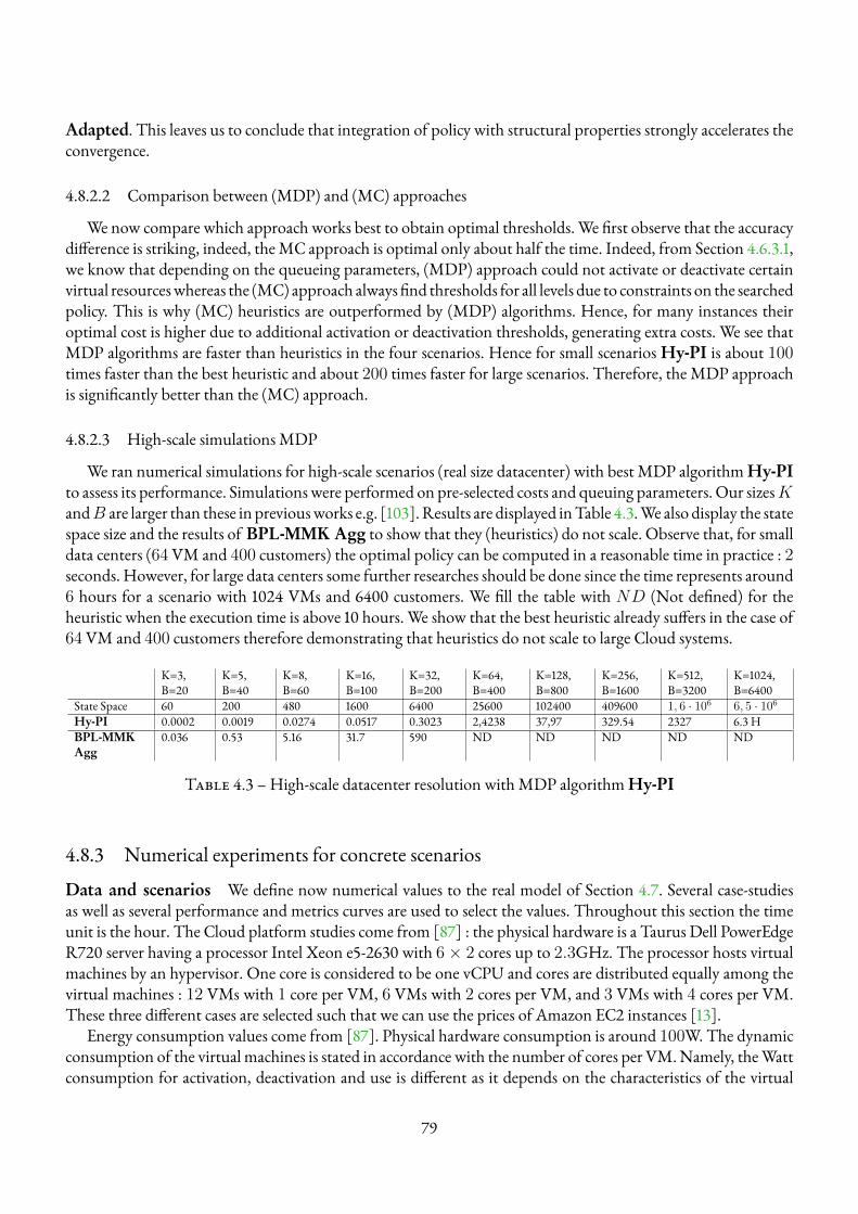
Adapted. This leaves us to conclude that integration of policy with structural properties strongly accelerates theconvergence.

4.8.2.2 Comparison between (MDP) and (MC) approaches

We now compare which approach works best to obtain optimal thresholds. We first observe that the accuracydifference is striking, indeed, theMC approach is optimal only about half the time. Indeed, from Section 4.6.3.1,we know that depending on the queueing parameters, (MDP) approach could not activate or deactivate certainvirtual resourceswhereas the (MC) approach always find thresholds for all levels due to constraints on the searchedpolicy. This is why (MC) heuristics are outperformed by (MDP) algorithms. Hence, for many instances theiroptimal cost is higher due to additional activation or deactivation thresholds, generating extra costs. We see thatMDP algorithms are faster than heuristics in the four scenarios. Hence for small scenarios Hy-PI is about 100times faster than the best heuristic and about 200 times faster for large scenarios. Therefore, the MDP approachis significantly better than the (MC) approach.

4.8.2.3 High-scale simulations MDP

We ran numerical simulations for high-scale scenarios (real size datacenter) with best MDP algorithmHy-PIto assess its performance. Simulations were performed on pre-selected costs and queuing parameters. Our sizesKandB are larger than these in previousworks e.g. [103].Results are displayed inTable 4.3.We also display the statespace size and the results of BPL-MMK Agg to show that they (heuristics) do not scale. Observe that, for smalldata centers (64VM and 400 customers) the optimal policy can be computed in a reasonable time in practice : 2seconds. However, for large data centers some further researches should be done since the time represents around6 hours for a scenario with 1024 VMs and 6400 customers. We fill the table with ND (Not defined) for theheuristic when the execution time is above 10 hours. We show that the best heuristic already suffers in the case of64 VM and 400 customers therefore demonstrating that heuristics do not scale to large Cloud systems.

K=3,B=20

K=5,B=40

K=8,B=60

K=16,B=100

K=32,B=200

K=64,B=400

K=128,B=800

K=256,B=1600

K=512,B=3200

K=1024,B=6400

State Space 60 200 480 1600 6400 25600 102400 409600 1, 6 · 106 6, 5 · 106

Hy-PI 0.0002 0.0019 0.0274 0.0517 0.3023 2,4238 37,97 329.54 2327 6.3 HBPL-MMKAgg

0.036 0.53 5.16 31.7 590 ND ND ND ND ND

Table 4.3 – High-scale datacenter resolution withMDP algorithmHy-PI

4.8.3 Numerical experiments for concrete scenarios

Data and scenarios We define now numerical values to the real model of Section 4.7. Several case-studiesas well as several performance and metrics curves are used to select the values. Throughout this section the timeunit is the hour. The Cloud platform studies come from [87] : the physical hardware is a Taurus Dell PowerEdgeR720 server having a processor Intel Xeon e5-2630 with 6 × 2 cores up to 2.3GHz. The processor hosts virtualmachines by an hypervisor. One core is considered to be one vCPU and cores are distributed equally among thevirtual machines : 12 VMs with 1 core per VM, 6 VMs with 2 cores per VM, and 3 VMs with 4 cores per VM.These three different cases are selected such that we can use the prices of Amazon EC2 instances [13].

Energy consumption values come from [87]. Physical hardware consumption is around 100W. The dynamicconsumption of the virtual machines is stated in accordance with the number of cores per VM.Namely, theWattconsumption for activation, deactivation and use is different as it depends on the characteristics of the virtual

79

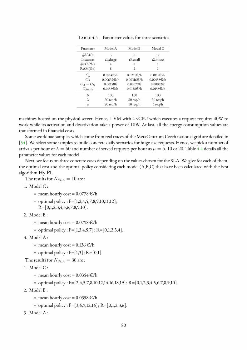
Table 4.4 – Parameter values for three scenarios

Parameter Model A Model B Model C

#VMs 3 6 12Instances a1.xlarge t3.small t2.micro#vCPUs 4 2 1RAM(Go) 8 2 1

Cp 0.0914e/h 0.0211e/h 0.0118e/hCS 0.00632e/h 0.00316e/h 0.00158e/h

CA = CD 0.00158e 0.00079e 0.00032eCStatic 0.0158e/h 0.0158e/h 0.0158e/h

B 100 100 100λ 50 req/h 50 req/h 50 req/hµ 20 req/h 10 req/h 5 req/h

machines hosted on the physical server. Hence, 1 VM with 4 vCPU which executes a request requires 40W towork while its activation and deactivation take a power of 10W. At last, all the energy consumption values aretransformed in financial costs.

Some workload samples which come from real traces of theMetaCentrum Czech national grid are detailed in[54].We select some samples to build concrete daily scenarios for huge size requests. Hence, we pick a number ofarrivals per hour of λ = 50 and number of served requests per hour as µ = 5, 10 or 20. Table 4.4 details all theparameter values for each model.

Next, we focus on three concrete cases depending on the values chosen for the SLA.We give for each of them,the optimal cost and the optimal policy considering each model (A,B,C) that have been calculated with the bestalgorithmHy-PI.

The results forNSLA = 10 are :1. Model C :∗ mean hourly cost = 0,0778 €/h∗ optimal policy : F=[1,2,4,5,7,8,9,10,11,12] ;R=[0,1,2,3,4,5,6,7,8,9,10].

2. Model B :∗ mean hourly cost = 0.0798 €/h∗ optimal policy : F=[1,3,4,5,7] ; R=[0,1,2,3,4].

3. Model A :∗ mean hourly cost = 0.136 €/h∗ optimal policy : F=[1,3] ; R=[0,1].

The results forNSLA = 30 are :1. Model C :∗ mean hourly cost = 0.0354 €/h∗ optimal policy : F=[2,4,5,7,8,10,12,14,16,18,19] ; R=[0,1,2,3,4,5,6,7,8,9,10].

2. Model B :∗ mean hourly cost = 0.0358 €/h∗ optimal policy : F=[3,6,9,12,16] ; R=[0,1,2,3,6].

3. Model A :

80

∗ mean hourly cost = 0.0397 €/h∗ optimal policy : F=[5,10] ; R=[0,1].

The results forNSLA = 50 are :1. Model C :∗ mean hourly cost = 0,0324 €/h∗ optimal policy : F=[3,5,7,9,11,14,17,21,26,30,34] ; R=[0,1,2,3,4,5,6,7,10,14,19].

2. Model B :∗ mean hourly cost = 0,0326 €/h∗ optimal policy : F=[4,8,13,21,30] ; R=[0,1,2,5,14].

3. Model A :∗ mean hourly cost = 0,0334 €/h∗ optimal policy : F=[9,22] ; R=[0,5].

We provide the mean run time of the best algorithm (Hy-PI) among concrete experiments : 0,00127 s forModel A; 0,0073 sec forModel B and 0,0372 sec forModel C. The optimal solution is computed in a short-timeand therefore can allow to recompute new policy when the demand is evolving, in order to dynamically adapt tothe need.

Mean global costs given SLA parameter or arrival rate From numerical simulations it could be noticedfirst that, for a fixed arrival rate λ, when the SLA is not so strict, then the cost decreases. Second that, when theresponse time set by the SLA rises, then the operating costs for the cloud providers are reduced. Indeed, providerswill pay fewer penalties to clients and fewer power bills for running VMs. On the other hand, we observe thatModel C is always better than Model B and Model A for any possible values of NSLA and for any values of λgiven a fixed SLA parameter. We can conclude that it is always better to decompose physical machine in severalvirtual resources, since it allows a more efficient resource allocation in dynamic scenario. Indeed, the more virtualresources you have, the less you will pay per utilisation since they require less CPU consumption. Moreover, itallows a more flexible system where you can easily adapt virtual resources to the demand.

Thresholds given SLA parameter or arrival rate We also observe thatModel C always activates a secondvirtual resource before the two other models B and A, for any fixed values of λ and SLA parameterNSLA. Fur-thermore, when the arrival rate λ is fixed, then all models will activate later when the SLA is less restrictive. Lastly,when the SLA parameter is fixed, we notice that the first activation threshold decreases when λ increases. Indeed,if the demand is growing, it requires more resources and requires faster activation of virtual resources.

Cost evaluation We display on Figure 4.12 an example (K = 8, B = 60) which exhibits the evolution ofthe financial cost per hour according to a givenNSLA, or to the load. We can see in the figure the impacts of suchparameters regarding performance and energy costs.

81

Figure 4.12 – Energy and performance costs given fixed SLA or arrival rate

Metrics and Performance We want to give some performance behaviour depending on some parameters,mostly how the financial cost per hour evolves depending on the givenNSLA, or on the load.The cost is calculatedwith theBPLAggheuristic for these examples.We can see inFig. 4.13 the impact of the SLAon the financial hourlycost for a cloud provider.

Figure 4.13 – Financial Cost for an hour depending on the SLA

82

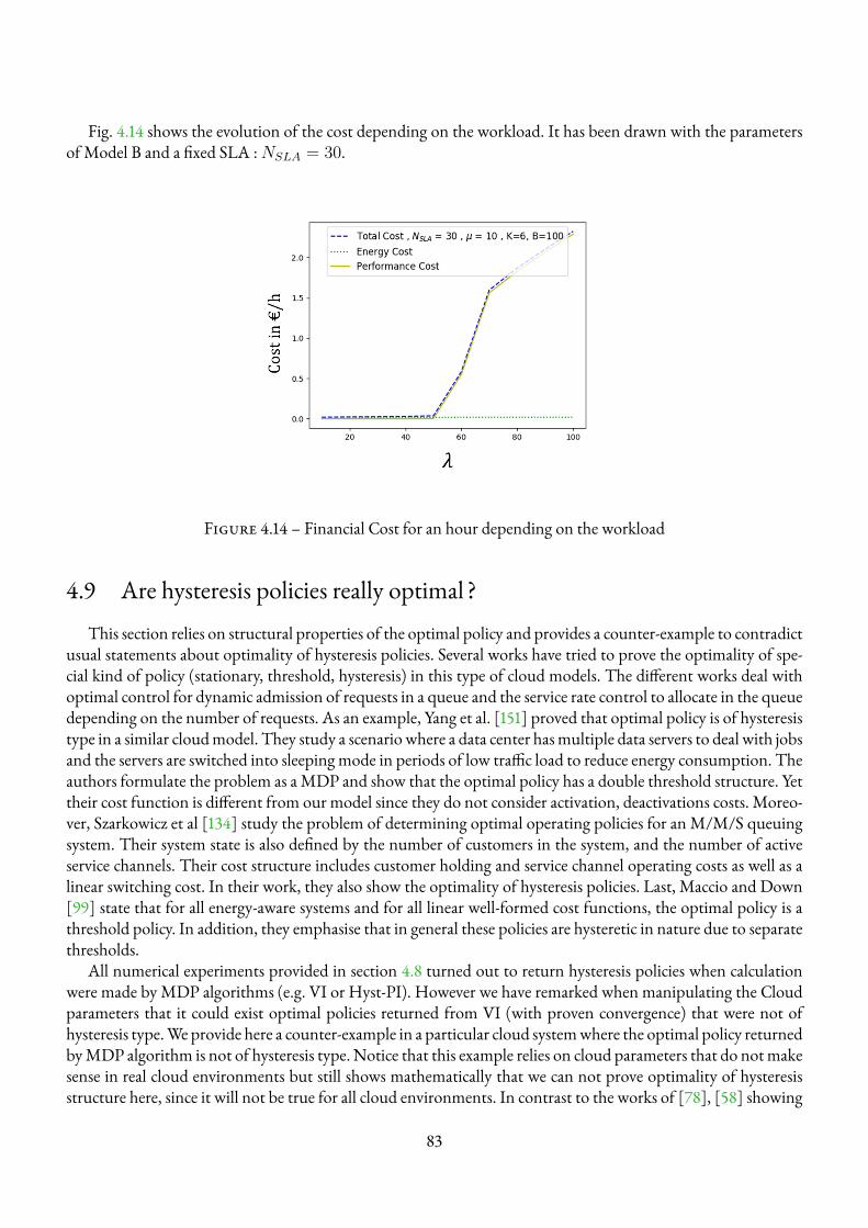
Fig. 4.14 shows the evolution of the cost depending on the workload. It has been drawn with the parametersof Model B and a fixed SLA :NSLA = 30.

Figure 4.14 – Financial Cost for an hour depending on the workload

4.9 Are hysteresis policies really optimal?This section relies on structural properties of the optimal policy and provides a counter-example to contradict

usual statements about optimality of hysteresis policies. Several works have tried to prove the optimality of spe-cial kind of policy (stationary, threshold, hysteresis) in this type of cloud models. The different works deal withoptimal control for dynamic admission of requests in a queue and the service rate control to allocate in the queuedepending on the number of requests. As an example, Yang et al. [151] proved that optimal policy is of hysteresistype in a similar cloudmodel. They study a scenario where a data center hasmultiple data servers to deal with jobsand the servers are switched into sleeping mode in periods of low traffic load to reduce energy consumption. Theauthors formulate the problem as aMDP and show that the optimal policy has a double threshold structure. Yettheir cost function is different from our model since they do not consider activation, deactivations costs. Moreo-ver, Szarkowicz et al [134] study the problem of determining optimal operating policies for an M/M/S queuingsystem. Their system state is also defined by the number of customers in the system, and the number of activeservice channels. Their cost structure includes customer holding and service channel operating costs as well as alinear switching cost. In their work, they also show the optimality of hysteresis policies. Last, Maccio and Down[99] state that for all energy-aware systems and for all linear well-formed cost functions, the optimal policy is athreshold policy. In addition, they emphasise that in general these policies are hysteretic in nature due to separatethresholds.

All numerical experiments provided in section 4.8 turned out to return hysteresis policies when calculationwere made by MDP algorithms (e.g. VI or Hyst-PI). However we have remarked when manipulating the Cloudparameters that it could exist optimal policies returned from VI (with proven convergence) that were not ofhysteresis type.We provide here a counter-example in a particular cloud systemwhere the optimal policy returnedbyMDP algorithm is not of hysteresis type. Notice that this example relies on cloud parameters that do notmakesense in real cloud environments but still shows mathematically that we can not prove optimality of hysteresisstructure here, since it will not be true for all cloud environments. In contrast to the works of [78], [58] showing

83

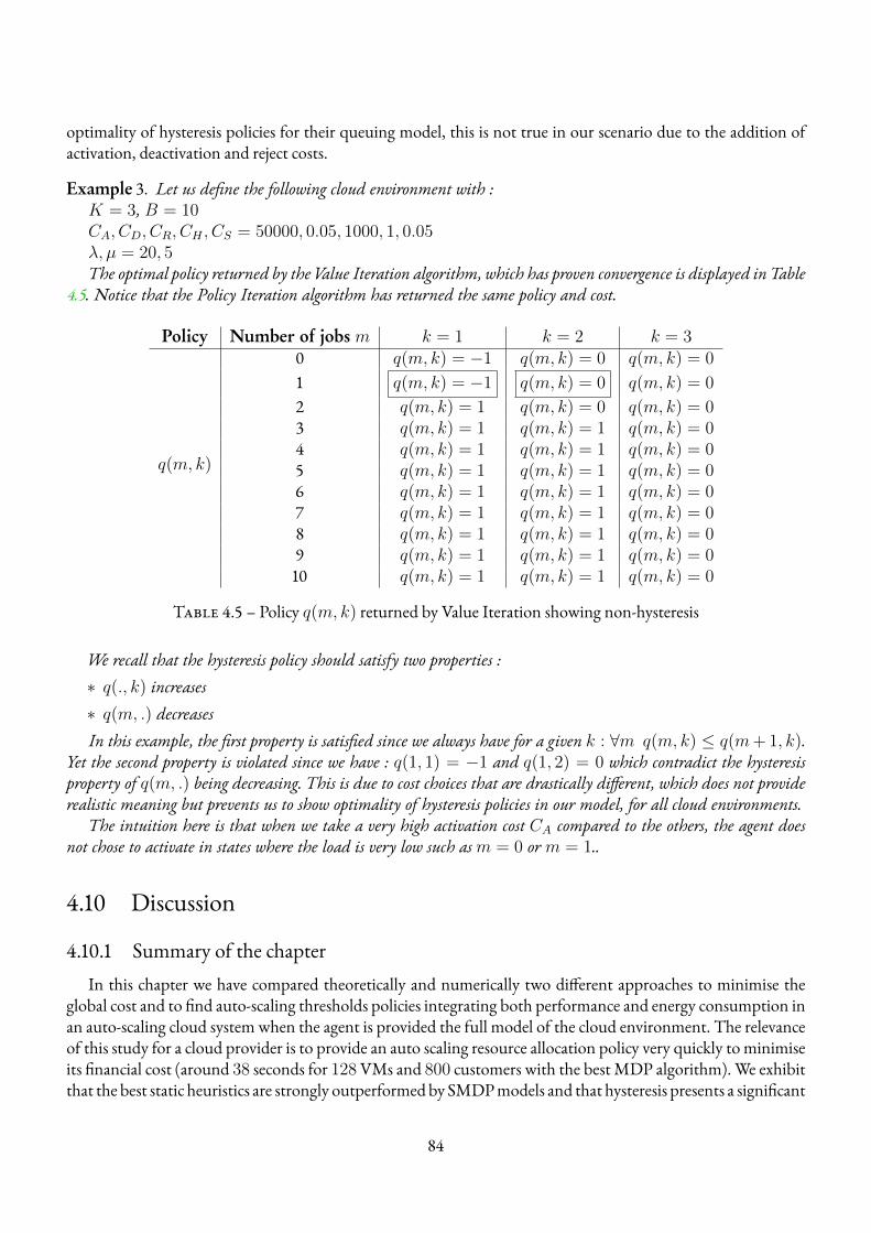
optimality of hysteresis policies for their queuing model, this is not true in our scenario due to the addition ofactivation, deactivation and reject costs.

Example 3. Let us define the following cloud environment with :K = 3, B = 10CA, CD, CR, CH , CS = 50000, 0.05, 1000, 1, 0.05λ, µ = 20, 5The optimal policy returned by the Value Iteration algorithm, which has proven convergence is displayed in Table

4.5. Notice that the Policy Iteration algorithm has returned the same policy and cost.

Policy Number of jobs m k = 1 k = 2 k = 3

q(m, k)

0 q(m, k) = −1 q(m, k) = 0 q(m, k) = 0

1 q(m, k) = −1 q(m, k) = 0 q(m, k) = 0

2 q(m, k) = 1 q(m, k) = 0 q(m, k) = 03 q(m, k) = 1 q(m, k) = 1 q(m, k) = 04 q(m, k) = 1 q(m, k) = 1 q(m, k) = 05 q(m, k) = 1 q(m, k) = 1 q(m, k) = 06 q(m, k) = 1 q(m, k) = 1 q(m, k) = 07 q(m, k) = 1 q(m, k) = 1 q(m, k) = 08 q(m, k) = 1 q(m, k) = 1 q(m, k) = 09 q(m, k) = 1 q(m, k) = 1 q(m, k) = 010 q(m, k) = 1 q(m, k) = 1 q(m, k) = 0

Table 4.5 – Policy q(m, k) returned by Value Iteration showing non-hysteresis

We recall that the hysteresis policy should satisfy two properties :∗ q(., k) increases∗ q(m, .) decreasesIn this example, the first property is satisfied since we always have for a given k : ∀m q(m, k) ≤ q(m+ 1, k).

Yet the second property is violated since we have : q(1, 1) = −1 and q(1, 2) = 0 which contradict the hysteresisproperty of q(m, .) being decreasing. This is due to cost choices that are drastically di�erent, which does not providerealistic meaning but prevents us to show optimality of hysteresis policies in our model, for all cloud environments.

The intuition here is that when we take a very high activation cost CA compared to the others, the agent doesnot chose to activate in states where the load is very low such asm = 0 orm = 1..

4.10 Discussion

4.10.1 Summary of the chapterIn this chapter we have compared theoretically and numerically two different approaches to minimise the

global cost and to find auto-scaling thresholds policies integrating both performance and energy consumption inan auto-scaling cloud system when the agent is provided the full model of the cloud environment. The relevanceof this study for a cloud provider is to provide an auto scaling resource allocation policy very quickly to minimiseits financial cost (around 38 seconds for 128VMs and 800 customers with the best MDP algorithm). We exhibitthat the best static heuristics are strongly outperformedby SMDPmodels and that hysteresis presents a significant

84

improvement. Although we have provided a counter-example with specific costs parameters for optimality ofhysteresis policies, it turns out that the optimal policies returned from numerical experiments were all hysteresiswhen taking consistent costs. From the numerical results, we show that the (MDP) approach is faster, but alsomuch more accurate. Moreover, it allows in some cases to define the number of resources needed to be allocatedon the physical server. Finally, we devised a realistic scenario of our cloudmodel we assessed our bestmethods andanalysed numerical results depending on SLA parameters and queueing parameters.

4.10.2 How to proceed with unknown statisticsThis chapter assumes that the autonomous agent fully knows the cloud environment and its dynamics, which

allows him to compute optimal policies. In real cloud systems, this hypothesis no longer holds since it is difficult tocapture queuing statistics such as arrival rates, service rates, etc. In this context we need to consider RL techniquesthat can learn in unknown environments.

85

CHAPTER 5

MODEL-BASEDREINFORCEMENT LEARNING FORMULTI-TIERNETWORK

The contributions of this chapter have been published in [142] :∗ Thomas Tournaire, Jeanne Barthélémy, Hind Castel-Taleb, Emmanuel Hyon. Reinforcement LearningwithModel-Based Approaches for Dynamic Resource Allocation in a TandemQueue. In Performance En-gineering and Stochastic Modeling. Springer International Publishing (ASMTA 21), 2021

The challenge for resource allocation in Cloud networks is that human experts do not easily know the exactstatistics of the system (arrivals, services) in real environments, because they evolve too quickly. Therefore a soft-ware agent does not possess any environment model for computation of the optimal policy. This requires theimplementation of Reinforcement Learning solutions. On the other hand, we are not sure that the practitionersapproaches are robust (often very experimental). Most of the work concerning RL for Cloud resource allocationis dedicated to model-free techniques such as Q-Learning [39] or Deep RL [113], but there exists no applicationof model-based techniques for such use-cases.

In this chapter, we want to evaluate the model-based RL approaches in the case of queuing networks, whichhas been little done so far.Moreover, we want to extend the range ofmodels studied (in Chapter IV to go beyondthe simple single multi-server model) to networks of several queues, which is better able to represent multi-tierarchitectures,whichhas alsonotbeendonemuch in the literature.Consequently,wenowassume that the learningagent does not carry the knowledge of theMDPmodel.The aim is therefore to adoptmodel-basedRLapproaches[106], especially Dyna architectures [8] and MDP online techniques [27] to assess their relevance, if ever, or toimprove them for dynamic resource allocation in queuing network systems. Moreover, we want to assess therobustness of such approaches in use-cases where there are arrivals that are bursty.

Therefore, the key contributions of this chapter are as follows :∗ We extend the one node scenario and propose two queuing systems for modelling three-tier architectures :tandemqueueingmodelwith Poisson arrivals, and thenwith (MMPP)Markovmodulated Poisson process ;∗ We integrate and discuss literature considerations regarding experimental comparison of reinforcement lear-ning algorithms;∗ We implement several versions of Dyna architecture and experimentally show that model-based reinfor-cement learning techniques can outperform classical model-free algorithms such as Q-Learning, on cloudauto-scaling applications ;

86

∗ Westudy the robustness ofRLalgorithmsonapartially observable systemwithMMPParrivalswhere arrivalrate is varying over time and is hidden to the agent. Nevertheless, we show that deterministic model-basedmethods suffer more than Q-learning in changing environments, while stochastic model-based methodssuch as MDP online can manage to have better performances.

The chapter first gives a more detailed overview of model-based reinforcement learning techniques, next pre-sents twoqueuingmodels to expressmulti-tier network architectures. Then it shows howwehave selectedmodel-based RL techniques by providing a general algorithm and how we parameterised them to compare with stateof the art model-free RL on the multi-tier cloud network. Last, we present comparison results between RL tech-niques on different cloud scenarios andparameters in a simulated environment, demonstrating the gain ofmodel-based RL techniques.

5.1 BackgroundModel-Based Reinforcement LearningNow, we present in more details the model-based RL framework introduced in Chapter III. We first describe

Dyna architectures [8] and prioritised replay techniques [122], state of the art MDP online techniques [27],[74], [109] and more advanced techniques following [106]. More precisely, we describe in this background sec-tion how the RL agent can learn the model of the world and how it can integrate learning and planning. Weencourage readers to check out the section 3.2.4.2 in Chapter III that discusses the planning phase and especiallyhow it is performed : Simulated trajectories, breadth and depth, dynamic programming. Broadly, the planningphase consists of simulating trajectories with the learned model for updating the value or policy functions andthe learning phase consists of extracting an environment model with dynamics and reward functions from col-lected data. Next, we provide more details about SoTAmodel-based RL algorithms regarding their learning andplanning processes.

5.1.1 Dyna architectures - Deterministic models and buffer replayDyna architectures [8] aims to improvemodel-freemethods by adding a supplementary planning phase where

the agent canupdatemoreoften its state-value function fromexperiences.The collected samples (st, at, rt+1, st+1)can be used to directly improve the value function and policy by storing them into a bu�er replay. This buffer re-play serves as a deterministic model of the world by predicting what will be the reward rt+1 and the next statest+1 when the agent selects action at in state st. The interaction between experience, model, values, and policyare depicted in Figure 5.1. The experience can improve value and policy functions either directly or indirectly viathe model.

Figure 5.1 – The reinforcement learning scheme in Dyna architectures (Figure from [8])

87

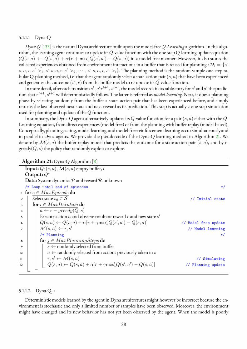
5.1.1.1 Dyna-Q

Dyna-Q [133] is the natural Dyna architecture built upon the model-freeQ-Learning algorithm. In this algo-rithm, the learning agent continues to update itsQ-value functionwith the one-stepQ-learning update equation(Q(s, a) ← Q(s, a) + α(r + max′aQ(s′, a′) − Q(s, a)) in a model-free manner. However, it also stores thecollected experiences obtained from environment interactions in a buffer that is reused for planning :Di = {<s, a, r, s′ >1, < s, a, r, s′ >2, · · · , < s, a, r, s′ >i}. The planning method is the random-sample one-step ta-bularQ-planningmethod, i.e. that the agent randomly select a state-action pair (s, a) that have been experiencedand generates the outcome (s′, r) from the buffer model to re-update itsQ-value function.

Inmore detail, after each transition st, atrt+1, st+1, themodel records in its table entry for st andat the predic-tion that rt+1, st+1 will deterministically follow. The latter is referred asmodel-learning. Next, it does a planningphase by selecting randomly from the buffer a state–action pair that has been experienced before, and simplyreturns the last-observed next state and next reward as its prediction. This step is actually a one-step simulationused for planning and update of theQ function.

In summary, the Dyna-Q agent alternatively updates itsQ-value function for a pair (s, a) either with theQ-Learning equation, from direct experiences (model-free) or from the planning with buffer replay (model-based).Conceptually, planning, acting,model-learning, andmodel-free reinforcement learning occur simultaneously andin parallel in Dyna agents. We provide the pseudo-code of the Dyna-Q learning method in Algorithm 21. Wedenote byM(s, a) the buffer replay model that predicts the outcome for a state-action pair (s, a), and by ε-greedy(Q, s) the policy that randomly exploit or explore.

Algorithm 21:Dyna-Q Algorithm [8]Input:Q0(s, a),M(s, a) empty buffer, εOutput:Q∗

Data: System dynamicsP and rewardR unknown/* Loop until end of episodes */

1 for e ∈MaxEpisode do2 Select state s0 ∈ S // Initial state3 for i ∈MaxIteration do4 a← ε− greedy(Q, s)5 Execute action a and observe resultant reward r and new state s′6 Q(s, a)← Q(s, a) + α[r + γmax′aQ(s′, a′)−Q(s, a)] // Model-free update7 M(s, a)← r, s′ // Model-learning

/* Planning */8 for j ∈MaxPlanningSteps do9 s← randomly selected from buffer

10 a← randomly selected from actions previously taken in s11 r, s′ ←M(s, a) // Simulating12 Q(s, a)← Q(s, a) + α[r + γmax′aQ(s′, a′)−Q(s, a)] // Planning update

5.1.1.2 Dyna-Q-+

Deterministic models learned by the agent in Dyna architectures might however be incorrect because the en-vironment is stochastic and only a limited number of samples have been observed. Moreover, the environmentmight have changed and its new behavior has not yet been observed by the agent. When the model is poorly

88

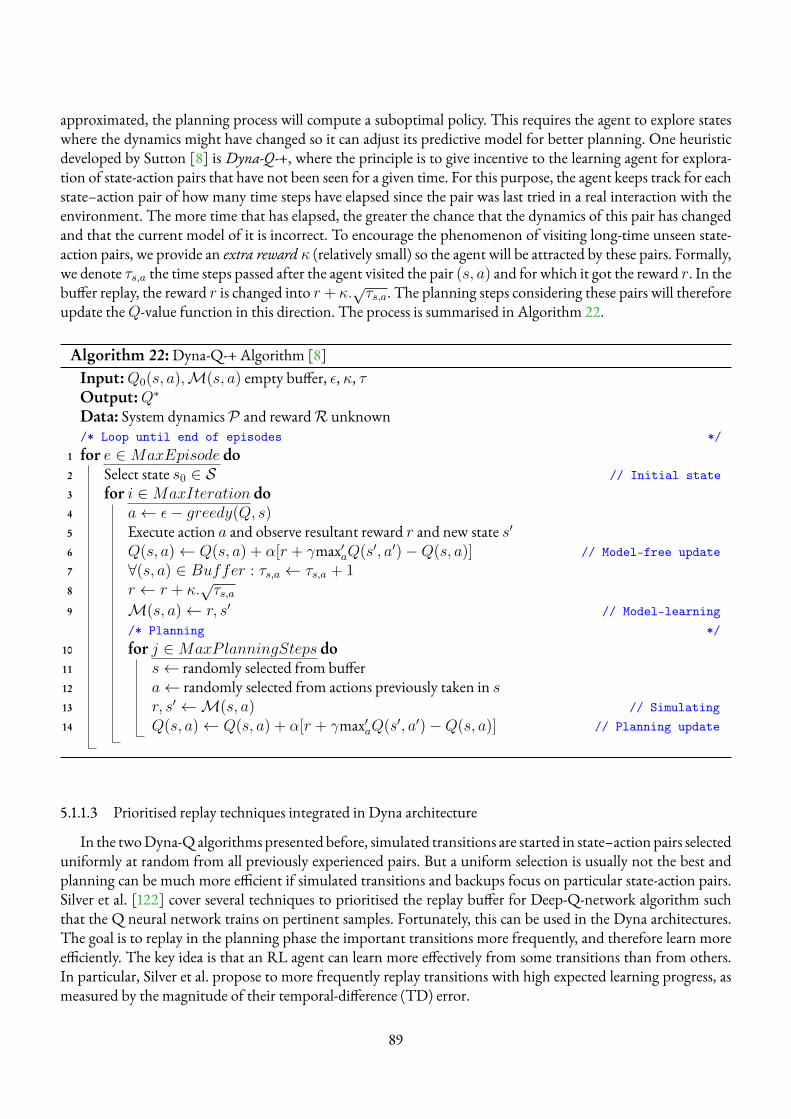
approximated, the planning process will compute a suboptimal policy. This requires the agent to explore stateswhere the dynamics might have changed so it can adjust its predictive model for better planning. One heuristicdeveloped by Sutton [8] is Dyna-Q-+, where the principle is to give incentive to the learning agent for explora-tion of state-action pairs that have not been seen for a given time. For this purpose, the agent keeps track for eachstate–action pair of how many time steps have elapsed since the pair was last tried in a real interaction with theenvironment. The more time that has elapsed, the greater the chance that the dynamics of this pair has changedand that the current model of it is incorrect. To encourage the phenomenon of visiting long-time unseen state-action pairs, we provide an extra reward κ (relatively small) so the agent will be attracted by these pairs. Formally,we denote τs,a the time steps passed after the agent visited the pair (s, a) and for which it got the reward r. In thebuffer replay, the reward r is changed into r+ κ.

√τs,a. The planning steps considering these pairs will therefore

update theQ-value function in this direction. The process is summarised in Algorithm 22.

Algorithm 22:Dyna-Q-+ Algorithm [8]Input:Q0(s, a),M(s, a) empty buffer, ε, κ, τOutput:Q∗

Data: System dynamicsP and rewardR unknown/* Loop until end of episodes */

1 for e ∈MaxEpisode do2 Select state s0 ∈ S // Initial state3 for i ∈MaxIteration do4 a← ε− greedy(Q, s)5 Execute action a and observe resultant reward r and new state s′6 Q(s, a)← Q(s, a) + α[r + γmax′aQ(s′, a′)−Q(s, a)] // Model-free update7 ∀(s, a) ∈ Buffer : τs,a ← τs,a + 18 r ← r + κ.

√τs,a

9 M(s, a)← r, s′ // Model-learning/* Planning */

10 for j ∈MaxPlanningSteps do11 s← randomly selected from buffer12 a← randomly selected from actions previously taken in s13 r, s′ ←M(s, a) // Simulating14 Q(s, a)← Q(s, a) + α[r + γmax′aQ(s′, a′)−Q(s, a)] // Planning update

5.1.1.3 Prioritised replay techniques integrated in Dyna architecture

In the twoDyna-Q algorithms presented before, simulated transitions are started in state–action pairs selecteduniformly at random from all previously experienced pairs. But a uniform selection is usually not the best andplanning can be much more efficient if simulated transitions and backups focus on particular state-action pairs.Silver et al. [122] cover several techniques to prioritised the replay buffer for Deep-Q-network algorithm suchthat the Q neural network trains on pertinent samples. Fortunately, this can be used in the Dyna architectures.The goal is to replay in the planning phase the important transitions more frequently, and therefore learn moreefficiently. The key idea is that an RL agent can learn more effectively from some transitions than from others.In particular, Silver et al. propose to more frequently replay transitions with high expected learning progress, asmeasured by the magnitude of their temporal-difference (TD) error.

89

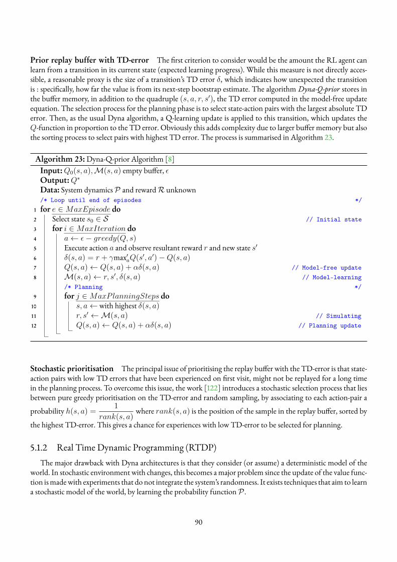
Prior replay buffer with TD-error The first criterion to consider would be the amount the RL agent canlearn from a transition in its current state (expected learning progress). While this measure is not directly acces-sible, a reasonable proxy is the size of a transition’s TD error δ, which indicates how unexpected the transitionis : specifically, how far the value is from its next-step bootstrap estimate. The algorithmDyna-Q-prior stores inthe buffer memory, in addition to the quadruple (s, a, r, s′), the TD error computed in the model-free updateequation. The selection process for the planning phase is to select state-action pairs with the largest absolute TDerror. Then, as the usual Dyna algorithm, a Q-learning update is applied to this transition, which updates theQ-function in proportion to the TD error. Obviously this adds complexity due to larger buffer memory but alsothe sorting process to select pairs with highest TD error. The process is summarised in Algorithm 23.

Algorithm 23:Dyna-Q-prior Algorithm [8]Input:Q0(s, a),M(s, a) empty buffer, εOutput:Q∗

Data: System dynamicsP and rewardR unknown/* Loop until end of episodes */

1 for e ∈MaxEpisode do2 Select state s0 ∈ S // Initial state3 for i ∈MaxIteration do4 a← ε− greedy(Q, s)5 Execute action a and observe resultant reward r and new state s′6 δ(s, a) = r + γmax′aQ(s′, a′)−Q(s, a)7 Q(s, a)← Q(s, a) + αδ(s, a) // Model-free update8 M(s, a)← r, s′, δ(s, a) // Model-learning

/* Planning */9 for j ∈MaxPlanningSteps do

10 s, a←with highest δ(s, a)11 r, s′ ←M(s, a) // Simulating12 Q(s, a)← Q(s, a) + αδ(s, a) // Planning update

Stochastic prioritisation The principal issue of prioritising the replay buffer with the TD-error is that state-action pairs with low TD errors that have been experienced on first visit, might not be replayed for a long timein the planning process. To overcome this issue, the work [122] introduces a stochastic selection process that liesbetween pure greedy prioritisation on the TD-error and random sampling, by associating to each action-pair a

probability h(s, a) =1

rank(s, a)where rank(s, a) is the position of the sample in the replay buffer, sorted by

the highest TD-error. This gives a chance for experiences with low TD-error to be selected for planning.

5.1.2 Real Time Dynamic Programming (RTDP)The major drawback with Dyna architectures is that they consider (or assume) a deterministic model of the

world. In stochastic environment with changes, this becomes amajor problem since the update of the value func-tion ismadewith experiments that do not integrate the system’s randomness. It exists techniques that aim to learna stochastic model of the world, by learning the probability functionP .

90

5.1.2.1 The primary concept : adaptive control

In 1999, Barto et al. [23] have covered the field of Dynamic Programming extensively. In their paper, theystudy Real Time Dynamic Programming techniques where a learning agent updates its value function or policywith DP techniques and always decide to act greedy, i.e. selecting a = argmaxaQ(s, a). In addition, they studywhat they call adaptive control, which is MDP scenario with incomplete information, i.e. where the agent doesnot know the dynamics of the system. Notice that this is in fact Reinforcement Learning. The authors claim thatit exists twomajor classes of adaptive control methods forMDPwith incomplete information :Bayesian methodsand non-Bayesian methods. The former (Bayesian) assumes a known a priori probability distribution over theclass of possible stochastic dynamic systems. As observations accumulate, this distribution is revised via Bayes’rule.

The latter (non-Bayesian) explicitly models the dynamic system being controlled and will be considered inthis chapter. They use system identification algorithms to update parameters whose values determine the currentsystem model. They typically make control decisions under the assumption that the current model is the truemodel of the system, i.e. they consider the confidence in their model used for planning. In a nutshell, these non-Bayesian methods estimate the unknown state-transition probabilities and immediate costs based on the historyof state transitions and immediate costs observed while the controller interacts with the environment. The mostcommon form of this identification approach is the maximum-likelihood technique [8], that allows to updatethe transition model by counting occurrences of visited state-action pairs (s, a) and (s, a, s′) :

P(s′|s, a) =](s, a, s′)

](s, a)

Last, it appears in these methods a conflict between conducting enough exploration to achieve model conver-gence and the objective of eventually following an optimal policy. This is related to the exploration-exploitationdilemma of the RL field. Adaptive optimal control algorithms require mechanisms for resolving these problems,but no mechanism is universally favored.

5.1.2.2 PAC-MDP algorithms

In this section, we give an overview of model-based RL techniques that ought to learn the stochastic modelof the dynamics and plan with DP techniques. These techniques directly inherit from the adaptive control idea.Most of the theoretical works about these algorithms study the sample complexity (Def. 9) of the methods [27,69, 74, 136]. The twomost known algorithms that exist are : E3 [74] for Explicit-Exploit-or-Explore andR-max[27]. They both have in common the learning of the probability distribution to performMDPplanningwith thelearned model. Note that planning can be done in two different ways : using dynamic programming algorithmssuch as Value Iteration [5] or using its model to generate new samples trajectories and update in a model-freefashion, such as Dyna mode. They also share a common property : both algorithms are PAC-MDP, for provablyapproximately correct in MDPs, i.e. that they have convergence bounds properties. To understand what is PAC-MDP, we first need to define Sample Complexity.Definition 9 (Sample Complexity [69]). LetM be an MDP with NS states, NA actions, discount factor γ ∈[0, 1) and amaximal rewarddenotedRmax > 0. LetAbe aRLalgorithmwhich acts in the environment, resultingin s0, a0, r0, s1, a1, r1, . . .

Let V At,M = E[

∞∑k=0

γkrt+k|s0, a0, r0, . . . , st−1, at−1, rt−1, st] and V ∗ the value function of the optimal po-

licy. Now, let ε > 0 be the accuracy and δ > 0 be an allowed probability of failure.The expression η(ε, δ,NS, NA, γ, Rmax) is a sample complexity bound for algorithm A if independently of

the choice of s0, the number of timesteps such that V At,M < V ∗ − ε is at most η(ε, δ,NS, NA, γ, Rmax) with

91

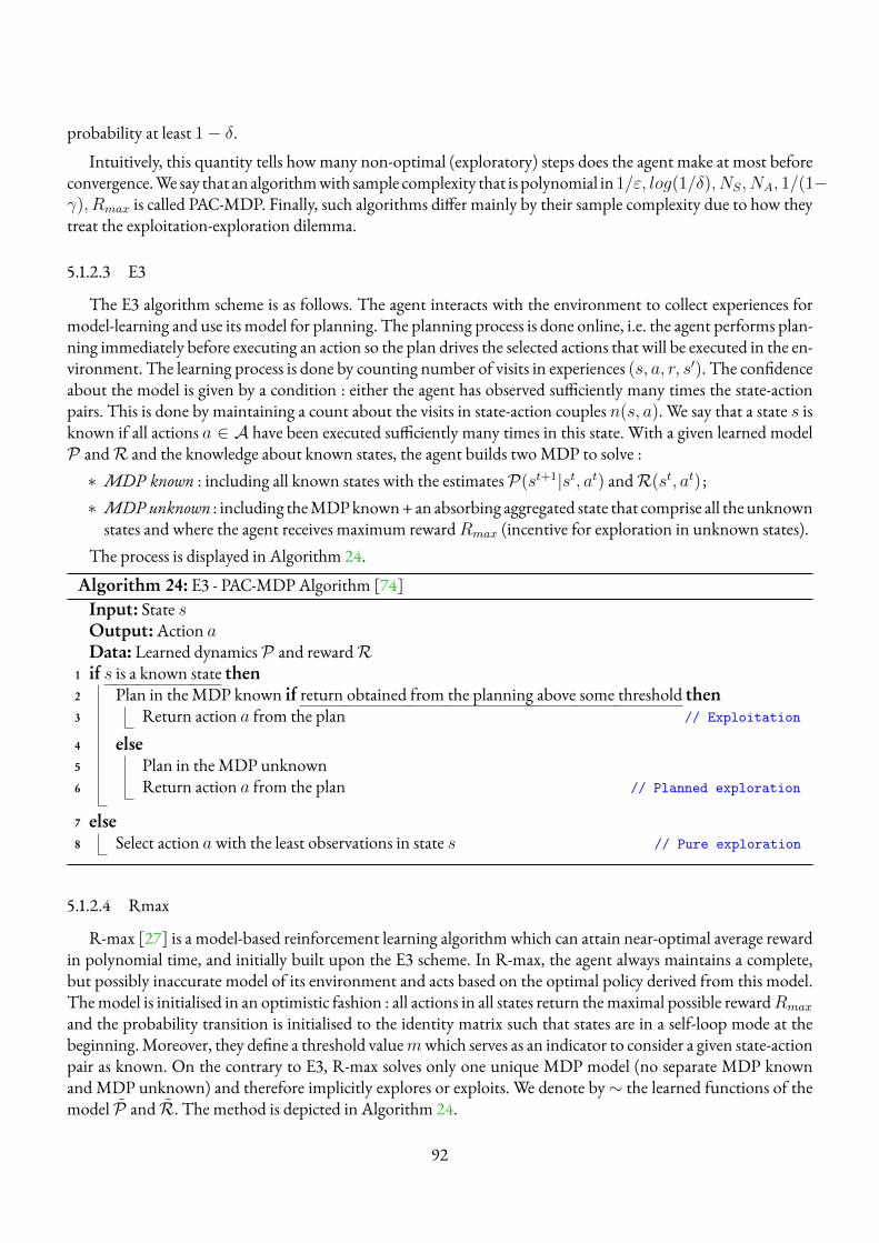
probability at least 1− δ.Intuitively, this quantity tells how many non-optimal (exploratory) steps does the agent make at most before

convergence.We say that an algorithmwith sample complexity that is polynomial in1/ε, log(1/δ), NS, NA, 1/(1−γ), Rmax is called PAC-MDP. Finally, such algorithms differ mainly by their sample complexity due to how theytreat the exploitation-exploration dilemma.

5.1.2.3 E3

The E3 algorithm scheme is as follows. The agent interacts with the environment to collect experiences formodel-learning and use its model for planning. The planning process is done online, i.e. the agent performs plan-ning immediately before executing an action so the plan drives the selected actions that will be executed in the en-vironment. The learning process is done by counting number of visits in experiences (s, a, r, s′). The confidenceabout the model is given by a condition : either the agent has observed sufficiently many times the state-actionpairs. This is done by maintaining a count about the visits in state-action couples n(s, a). We say that a state s isknown if all actions a ∈ A have been executed sufficiently many times in this state. With a given learned modelP andR and the knowledge about known states, the agent builds twoMDP to solve :∗ MDP known : including all known states with the estimatesP(st+1|st, at) andR(st, at) ;∗ MDPunknown : including theMDPknown+an absorbing aggregated state that comprise all the unknownstates and where the agent receives maximum rewardRmax (incentive for exploration in unknown states).

The process is displayed in Algorithm 24.

Algorithm 24: E3 - PAC-MDP Algorithm [74]Input: State sOutput:Action aData: Learned dynamicsP and rewardR

1 if s is a known state then2 Plan in the MDP known if return obtained from the planning above some threshold then3 Return action a from the plan // Exploitation

4 else5 Plan in the MDP unknown6 Return action a from the plan // Planned exploration

7 else8 Select action awith the least observations in state s // Pure exploration

5.1.2.4 Rmax

R-max [27] is a model-based reinforcement learning algorithmwhich can attain near-optimal average rewardin polynomial time, and initially built upon the E3 scheme. In R-max, the agent always maintains a complete,but possibly inaccurate model of its environment and acts based on the optimal policy derived from this model.Themodel is initialised in an optimistic fashion : all actions in all states return themaximal possible rewardRmax

and the probability transition is initialised to the identity matrix such that states are in a self-loop mode at thebeginning.Moreover, they define a threshold valuemwhich serves as an indicator to consider a given state-actionpair as known. On the contrary to E3, R-max solves only one unique MDP model (no separate MDP knownand MDP unknown) and therefore implicitly explores or exploits. We denote by∼ the learned functions of themodel P and R. The method is depicted in Algorithm 24.

92

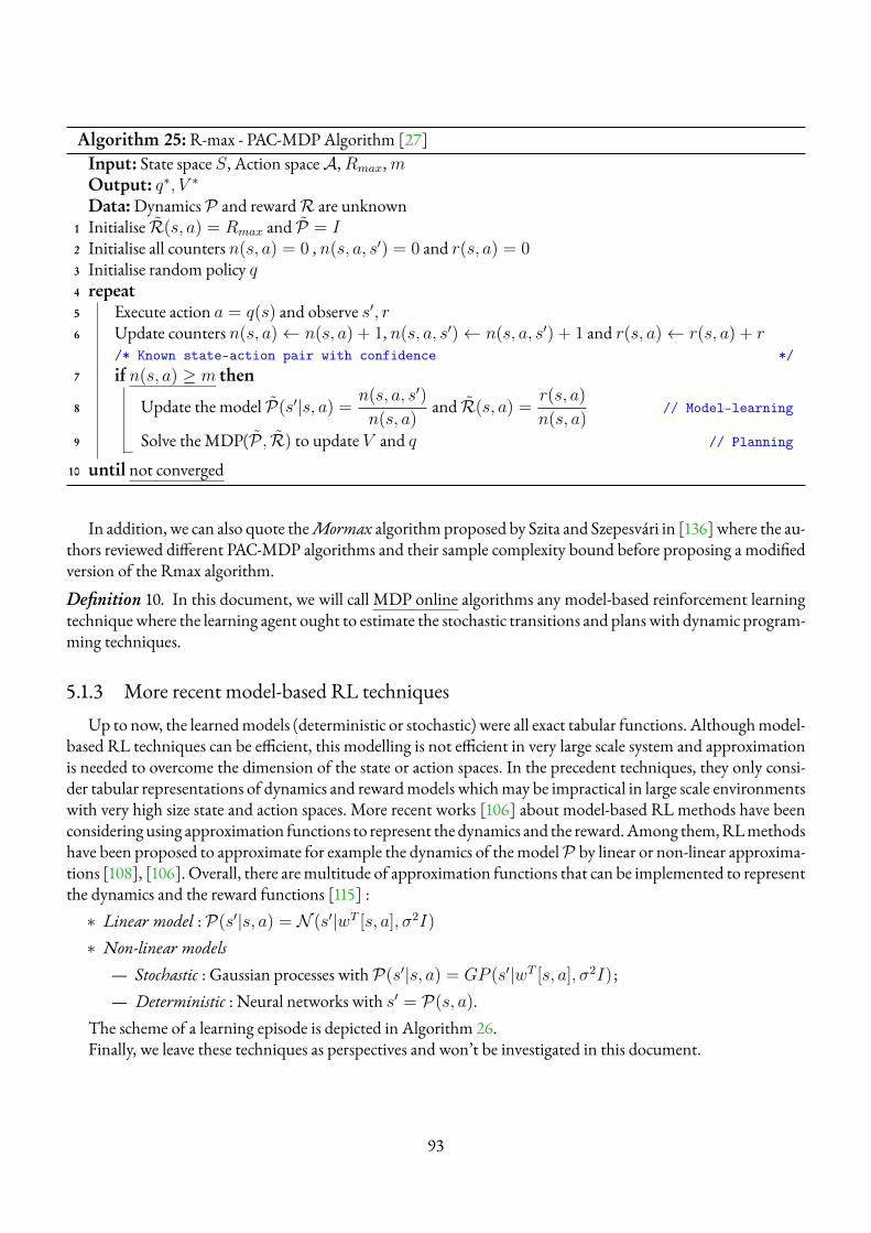
Algorithm 25:R-max - PAC-MDP Algorithm [27]Input: State space S, Action spaceA,Rmax,mOutput: q∗, V ∗

Data:DynamicsP and rewardR are unknown1 Initialise R(s, a) = Rmax and P = I2 Initialise all counters n(s, a) = 0 , n(s, a, s′) = 0 and r(s, a) = 03 Initialise random policy q4 repeat5 Execute action a = q(s) and observe s′, r6 Update counters n(s, a)← n(s, a) + 1, n(s, a, s′)← n(s, a, s′) + 1 and r(s, a)← r(s, a) + r

/* Known state-action pair with confidence */7 if n(s, a) ≥ m then

8 Update the model P(s′|s, a) =n(s, a, s′)

n(s, a)and R(s, a) =

r(s, a)

n(s, a)// Model-learning

9 Solve the MDP(P , R) to update V and q // Planning

10 until not converged

In addition, we can also quote theMormax algorithmproposed by Szita and Szepesvári in [136] where the au-thors reviewed different PAC-MDP algorithms and their sample complexity bound before proposing a modifiedversion of the Rmax algorithm.Definition 10. In this document, we will call MDP online algorithms any model-based reinforcement learningtechniquewhere the learning agent ought to estimate the stochastic transitions and plans with dynamic program-ming techniques.

5.1.3 More recent model-based RL techniquesUp to now, the learnedmodels (deterministic or stochastic) were all exact tabular functions. Althoughmodel-

based RL techniques can be efficient, this modelling is not efficient in very large scale system and approximationis needed to overcome the dimension of the state or action spaces. In the precedent techniques, they only consi-der tabular representations of dynamics and rewardmodels whichmay be impractical in large scale environmentswith very high size state and action spaces. More recent works [106] about model-based RL methods have beenconsideringusing approximation functions to represent the dynamics and the reward.Among them,RLmethodshave been proposed to approximate for example the dynamics of themodelP by linear or non-linear approxima-tions [108], [106]. Overall, there aremultitude of approximation functions that can be implemented to representthe dynamics and the reward functions [115] :∗ Linear model :P(s′|s, a) = N (s′|wT [s, a], σ2I)

∗ Non-linear models— Stochastic : Gaussian processes withP(s′|s, a) = GP (s′|wT [s, a], σ2I) ;— Deterministic : Neural networks with s′ = P(s, a).

The scheme of a learning episode is depicted in Algorithm 26.Finally, we leave these techniques as perspectives and won’t be investigated in this document.

93

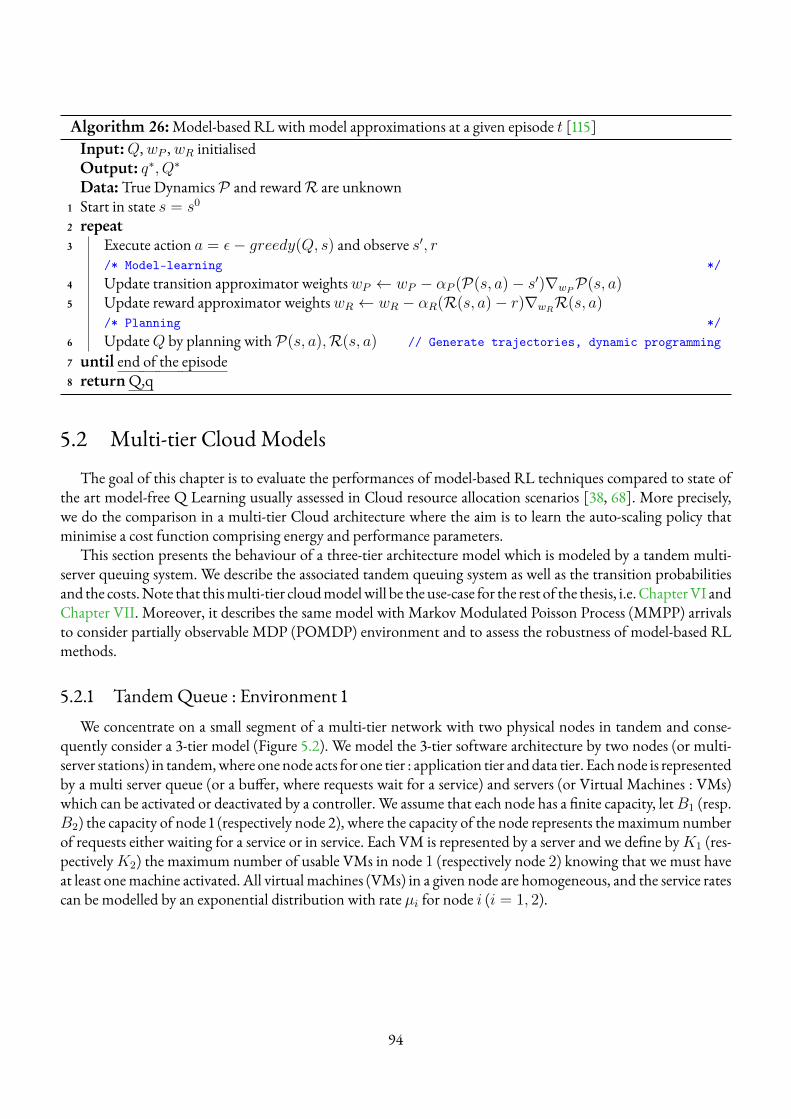
Algorithm 26:Model-based RL with model approximations at a given episode t [115]Input:Q,wP ,wR initialisedOutput: q∗, Q∗

Data:True DynamicsP and rewardR are unknown1 Start in state s = s0

2 repeat3 Execute action a = ε− greedy(Q, s) and observe s′, r

/* Model-learning */4 Update transition approximator weightswP ← wP − αP (P(s, a)− s′)∇wPP(s, a)5 Update reward approximator weightswR ← wR − αR(R(s, a)− r)∇wRR(s, a)

/* Planning */6 UpdateQ by planning withP(s, a),R(s, a) // Generate trajectories, dynamic programming

7 until end of the episode8 returnQ,q

5.2 Multi-tier CloudModelsThe goal of this chapter is to evaluate the performances of model-based RL techniques compared to state of

the art model-free Q Learning usually assessed in Cloud resource allocation scenarios [38, 68]. More precisely,we do the comparison in a multi-tier Cloud architecture where the aim is to learn the auto-scaling policy thatminimise a cost function comprising energy and performance parameters.

This section presents the behaviour of a three-tier architecture model which is modeled by a tandem multi-server queuing system. We describe the associated tandem queuing system as well as the transition probabilitiesand the costs.Note that thismulti-tier cloudmodelwill be the use-case for the rest of the thesis, i.e. ChapterVI andChapter VII. Moreover, it describes the same model with Markov Modulated Poisson Process (MMPP) arrivalsto consider partially observable MDP (POMDP) environment and to assess the robustness of model-based RLmethods.

5.2.1 TandemQueue : Environment 1We concentrate on a small segment of a multi-tier network with two physical nodes in tandem and conse-

quently consider a 3-tier model (Figure 5.2). We model the 3-tier software architecture by two nodes (or multi-server stations) in tandem,where onenode acts for one tier : application tier anddata tier. Eachnode is representedby a multi server queue (or a buffer, where requests wait for a service) and servers (or Virtual Machines : VMs)which can be activated or deactivated by a controller. We assume that each node has a finite capacity, letB1 (resp.B2) the capacity of node 1 (respectively node 2), where the capacity of the node represents themaximumnumberof requests either waiting for a service or in service. Each VM is represented by a server and we define byK1 (res-pectivelyK2) the maximum number of usable VMs in node 1 (respectively node 2) knowing that we must haveat least onemachine activated. All virtual machines (VMs) in a given node are homogeneous, and the service ratescan be modelled by an exponential distribution with rate µi for node i (i = 1, 2).

94

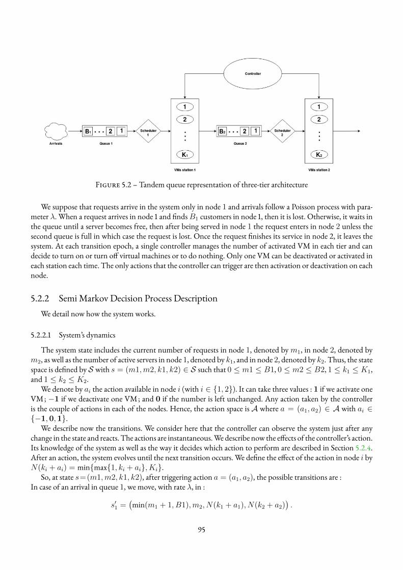
Figure 5.2 – Tandem queue representation of three-tier architecture

We suppose that requests arrive in the system only in node 1 and arrivals follow a Poisson process with para-meter λ. When a request arrives in node 1 and findsB1 customers in node 1, then it is lost. Otherwise, it waits inthe queue until a server becomes free, then after being served in node 1 the request enters in node 2 unless thesecond queue is full in which case the request is lost. Once the request finishes its service in node 2, it leaves thesystem. At each transition epoch, a single controller manages the number of activated VM in each tier and candecide to turn on or turn off virtual machines or to do nothing. Only one VM can be deactivated or activated ineach station each time. The only actions that the controller can trigger are then activation or deactivation on eachnode.

5.2.2 Semi Markov Decision Process DescriptionWe detail now how the system works.

5.2.2.1 System’s dynamics

The system state includes the current number of requests in node 1, denoted bym1, in node 2, denoted bym2, as well as the number of active servers in node 1, denoted by k1, and in node 2, denoted by k2. Thus, the statespace is defined by S with s = (m1,m2, k1, k2) ∈ S such that 0 ≤ m1 ≤ B1, 0 ≤ m2 ≤ B2, 1 ≤ k1 ≤ K1,and 1 ≤ k2 ≤ K2.

We denote by ai the action available in node i (with i ∈ {1, 2}). It can take three values : 1 if we activate oneVM; −1 if we deactivate one VM; and 0 if the number is left unchanged. Any action taken by the controlleris the couple of actions in each of the nodes. Hence, the action space isA where a = (a1, a2) ∈ A with ai ∈{−1,0,1}.

We describe now the transitions. We consider here that the controller can observe the system just after anychange in the state and reacts. The actions are instantaneous.Wedescribe now the effects of the controller’s action.Its knowledge of the system as well as the way it decides which action to perform are described in Section 5.2.4.After an action, the system evolves until the next transition occurs. We define the effect of the action in node i byN(ki + ai) = min{max{1, ki + ai}, Ki}.

So, at state s=(m1,m2, k1, k2), after triggering action a = (a1, a2), the possible transitions are :In case of an arrival in queue 1, we move, with rate λ, in :

s′1 =(min(m1 + 1, B1),m2, N(k1 + a1), N(k2 + a2)

).

95

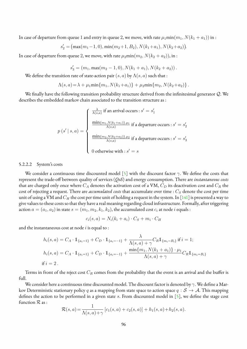
In case of departure from queue 1 and entry in queue 2, we move, with rate µ1min(m1, N(k1 + a1)) in :

s′2 =(max(m1−1, 0),min(m2+1, B2), N(k1+a1), N(k2+a2)

).

In case of departure from queue 2, we move, with rate µ2min(m2, N(k2 + a2)), in :

s′3 = (m1,max(m2 − 1, 0), N(k1 + a1), N(k2 + a2)) .

We define the transition rate of state-action pair (s, a) by Λ(s, a) such that :

Λ(s, a)=λ+ µ1min{m1, N(k1+a1)}+ µ2min{m2, N(k2+a2)} .

We finally have the following transition probability structure derived from the infinitesimal generatorQ. Wedescribes the embedded markov chain associated to the transition structure as :

p (s′ | s, a) =

λΛ(s,a)

if an arrival occurs : s′ = s′1

min{m1,N(k1+a1)}.µ1Λ(s,a)

if a departure occurs : s′ = s′2

min{m2,N(k2+a2)}.µ2Λ(s,a)

if a departure occurs : s′ = s′3

0 otherwise with : s′ = s

5.2.2.2 System’s costs

We consider a continuous time discounted model [5] with the discount factor γ. We define the costs thatrepresent the trade-off between quality of services (QoS) and energy consumption. There are instantaneous coststhat are charged only once where CA denotes the activation cost of a VM, CD its deactivation cost and CR thecost of rejecting a request. There are accumulated costs that accumulate over time : CS denote the cost per timeunit of using a VMandCH the cost per time unit of holding a request in the system. In [141] is presented away togive values to these costs so that they have a realmeaning regarding cloud infrastructure. Formally, after triggeringaction a = (a1, a2) in state s = (m1,m2, k1, k2), the accumulated cost ci at node i equals :

ci(s, a) = Ni(ki + ai) · CS +mi · CHand the instantaneous cost at node i is equal to :

hi(s, a) = CA · 1{ai=1} + CD · 1{ai=−1} +λ

Λ(s, a) + γCR1{mi=Bi} if i = 1;

hi(s, a) = CA · 1{ai=1} + CD · 1{ai=−1} +min{m1, N(k1 + a1)} · µ1

Λ(s, a) + γCR1{mi=Bi}

if i = 2 .

Terms in front of the reject cost CR comes from the probability that the event is an arrival and the buffer isfull.

We consider here a continuous time discountedmodel. The discount factor is denoted by γ. We define aMar-kov Deterministic stationary policy q as a mapping from state space to action space q : S → A. This mappingdefines the action to be performed in a given state s. From discounted model in [5], we define the stage costfunctionR as :

R(s, a)=1

Λ(s, a)+γ[c1(s, a) + c2(s, a)] + h1(s, a)+h2(s, a).

96

5.2.2.3 Uniformisation

Most reinforcement learningmodels andmore precisely model-based applications deal with discrete time sce-nario. In order to handle this control model with anRL approach we will uniformise the continuous timemodelto obtain a discrete time model on which we can use standard methods of R.L. some of which are already imple-mented in R.L. libraries.

The way to proceed (see details in chapter 11 of [5]) is first to define a constant which is finite and larger orequal to the maximum transition rate. Here we take Λ = λ + K1 · µ1 + K2 · µ2. Then, for each state-actioncouple (s, a) we add a transition associated with a pseudo event so that the process remains in the same state s.In (s, a), this transition has rate Λ − (Λ(s, a)) thus the transition rate is constant with rate Λ regardless (s, a).The transition probabilities in the uniformised model are denoted by p(s′|(s, a)) and are given by :

Λ× p(s′|s, a) =

λ if s′ = s′1µ1min{m1, N(k1 + a1)} if s′ = s′2µ2min{m2, N(k2 + a2)} if s′ = s′3(Λ− Λ(s, a)

)when s′ = s

0 otherwise .

The states s′2 and s′3 are defined in the system’s dynamic part above. It exists only few states for whichwe naturallyjump into the same state (i.e. s′ = s).These states are such thatm1 = B1 andN(k1+a1) = k1 andN(k2+a2) =k2 and the event is an arrival. In such cases the transition probability toward s′ = s is equal to Λ − (Λ(s, a) −λ)/Λ, see [5].The stage costs also need to be modified. Now they are given in the discounted model by :

R(s, a) =Λ(s, a) + γ

Λ + γR(s, a) .

Then the Bellman Equation of such a model is :

V ∗(s) = mina∈A(R(s, a) +

Λ

Λ + γ

∑s′

p(s′|(s, a))V ∗(s′)).

Note that this equation is never solved in R.L. methods but we solve it in our numerical experiments to assess theprecision of the algorithms. Indeed its solution is the theoretical optimal value.

5.2.3 MMPP TandemQueue model : Environment 2In this section we want to assess robustness of reinforcement learning algorithms and especially model-based

algorithms. For this purpose, we consider variations in the requests arrival rate with MarkovModulated PoissonProcess system. However, these variations would be remained ignored by the agent which expects a constantintensity.We studyhow the algorithms react to sudden and large increases of packet arrivals and if they canquicklyadapt their policy to overcome bursts traffic. This is a key element in network inwhich statistics are often not veryprecise. This is all the more important for model-based methods, since it was quoted in [46] that offline policiesmight no be adequate as soon as there exist changes in the dynamics of the environment. It is believed that this lackof flexibility comes from the offline learning of the policy in model-based methods and that this offline learningis done from a predefined model which does not allow to adapt to changes in the dynamics of the environment.

97

5.2.3.1 MarkovModulated Poisson Process

Wemodify now the arrival process.Wewant to integrate a variability feature andwe consider aMarkovmodu-lated Poisson process (MMPP) where arrival rates vary over time. The process switches between different Poissonprocess which differ by their intensity indicated by their arrival rate λj . We assume we have J phases, each ofthem corresponding to a specific arrival rate λj . The switch between the phases follows a continuous time Mar-kov chain. It is represented by a birth and death process [125] with ratesQ. Wemove from phase j to phase j+ 1with rate qj,j+1 and fromphase j to phase j−1with rate qj,j−1. Usually [125], qj,j+1 and qj,j−1 for all j aremuchsmaller than arrival rates {λj}j . We extend the previous state s = (m1,m2, k1, k2) to a new state representationintegrating the phase in the SMDP :

s = (j,m1,m2, k1, k2)

with λj the current arrival rate in phase j.In ourmodel, we assume that J = 2. The first phase is considered as normal and the second phase called burst

is a phase with a very high intensity. We denote by q1,2 the transition rate from phase 1 to phase 2 and by q2,1 thetransition rate from phase 2 to phase 1.

MMPP System’s dynamics Weneed to integrate new phase transitions in thewhole environment dynamics.Under given phases j, we have the dynamics detailed in section 5.2.2.1 for arrival rate λj . The system can havetwo additional events corresponding to a change of its phase, i.e. the current arrival rate changes. Thus :We move :

from s =(j,m1,m2, N(k1+a1), N(k2+a2))with rate qj,j+1 to s′4 = (j+1,m1,m2, N(k1+a1), N(k2+

a2));

from s =(j,m1,m2, N(k1+a1), N(k2+a2))with rate qj,j−1 to s′5 = (j−1,m1,m2, N(k1+a1), N(k2+

a2)).

We define the new transition rate by state by Λ(s, a) such that :Λ(s, a) = qj,j+1 + qj,j−1 + λj + µ1min{m1, N(k1 +a1)} + µ2min{m2, N(k2 +a2)}. The cost function

remains the same since variation in the arrival rate does not induce additional costs.

MMPP Uniformisation For the MMPP uniformisation process we take Λ = maxjqj,j+1 + maxjqj,j−1 +maxjλj+K1 ·µ1 +K2 ·µ2. Then, for each state-action couple (s, a)we add a transition associatedwith a pseudoevent so that the process remains in the same state s. In (s, a), this transition has rate Λ− Λ(s, a) such that thetransition rate of the whole point process is constant with rate Λ regardless (s, a). The transition probabilities inthe uniformised model are denoted by p(s′|(s, a)) and satisfy :

Λ× p(s′|s, a) =

λj if s′ = s′1µ1 ·min{m1, N(k1 + a1)} if s′ = s′2µ2 ·min{m2, N(k2 + a2)} if s′ = s′3qj,j+1 if s′ = s′4qj,j−1 if s′ = s′5(Λ− Λ(s, a)

)when s′ = s

0 otherwise

.

Similarly as before, the states for which it exists a natural jump into the same state are those already described forwhich the event is an arrival. In such a case the transition probability toward s′ = s is equal to(

Λ− (Λ(s, a)− λj))/Λ.

98

5.2.4 Simulated SMDP environment and objective function for RL agentNow, we first provide how the agent perceives and interacts with the simulated environment, next display the

objective function that the learning agent ought to optimise.

5.2.4.1 Simulated SMDP environment and agent’s observation

We are dealing with a reinforcement learning model therefore the uniformised model of Section 5.2 is notknownbutonly experiencedby the controller. Indeed, the controller doesnothave any information aboutqueuingstatistics (arrival rate, etc.), therefore does not know the dynamics of the system. The environment has state spaceS and action spaceA similarly to the SMDPmodel. When the agent interacts with the environment, the SMDPmodel is simulated. It will behave by returning a state, sampled according to the transition probabilities P , andreturn the costsR(s, a). The cost and the new state are the only information that the controller will discover.

For the partially observable scenario described with theMMPP environment, the agent’s observation remainsthe same.As already said,we consider amodelwith variation of arrivals, thus the systembehaves as the SMDPdes-cribed just above and the system state is described by s = (j,m1,m2, k1, k2). However, we assume that the lear-ning agent ignores these variations. Hence, the system can be only observed partially and the environment state isdescribed by o = (m1,m2, k1, k2). In this way, the two system states (1,m1,m2, k1, k2) and (2,m1,m2, k1, k2)translate in the same environment state (m1,m2, k1, k2). The goal is to assess and compare the robustness of rein-forcement learning algorithms in the contextwhere the agent does not have knowledge of an explanatory variable.

Overall, we consider in this work countable discrete state space where the agent can evaluate value function,policy, transition and reward matrices with tabular forms. We want to minimise the expected discounted cumu-lative costs.

5.2.4.2 Objective function

We search the best policy q tominimise the expected discounted expected reward, therefore the objective func-tion is :

V ∗(s) = minqEq

[∞∑k=0

exp−γtk R(sk, q(sk)) | s0 = s

], (5.1)

with tk the epoch and sk the state of the kth transition.

5.3 Generalisation and Selection of Model-based Reinforcement LearningAlgorithms

In this chapter,wewant to compare several tabularmodel-basedRLalgorithmswith state of the artmodel-freealgorithm, such as tabular Q-Learning, in the tandem queue scenario. We want to assess if the learning agent canbenefit from learning themodel underlying the environment and if it is worth increasing the complexity to speedup learning convergence. After selecting the model-based RL techniques, we present an aggregated pseudo-codeformodel-based reinforcement learning anddiscuss theparameterisationof themethods,with respect to the itemspresented in Chapter III (breadth planning, depth planning, integration learning and planning, etc.). Moreover,we assume here that the reward function is provided to the agent, thus it only needs to update the dynamicmodelP .

99

5.3.1 Algorithms selectionFor comparison of model-based Reinforcement Learning with SoTAmodel-free techniques we have selected

the following methods :∗ Deterministic models - bu�er replay : Dyna architectures withDyna-Q,Dyna-Q-+ and Dyna-Q with prio-ritisation on the TD-error in the buffer replay, denotedDyna-Q-prior ;∗ Stochastic model :MDP online, an algorithm that learns the stochastic transitions to performDP algorithmssuch as VI or PI, inspired by Rmax and E3 techniques.

In this part,wedescribe the different elements onwhichwe canoperate in themodel-based algorithms. Indeed,many factors affect the quality of learning : the frequency of model update, the frequency of planning, and theplanning itself (breadth, depth, etc.).

5.3.2 Learning processThe learning process is different in deterministic and stochastic models. For Dyna architectures, the learning

process consists of storing the experiments (s, a, r, s′) into the replay buffer, and for the prioritised version toadd the TD-error for each tuple δ(s, a) in order to sort the samples for planning. On the other hand, the learningin the stochastic process is made by counting occurrences of samples and updating the transition probability forstate-action pairs as explained in Section 5.1 [23] :

P(s′|s, a) =](s, a, s′)

](s, a)

5.3.3 Planning processWe encourage the readers to take over Figure 3.3 to see the difference between different approaches. In the

Dyna architectures during the planning phase, the learning agent reuse its past experiences to simulate trajecto-ries for supplementary update of theQ-value function. As we have seen in Section 5.1, the planning process hasseveral parameters, regarding the number of trajectories it generates, the breadth and depth of the process. In ourimplementation, the agent will generate several rollouts starting from a state s encountered in the buffer and willproceed a single time step (depth ξ equal to 1) by retrieving the next state s′ and reward r from the memory. Thenumber of rollouts (or breadth) is denoted ζ . InDyna-Q andDyna-Q-+, the sampling of state s is done randomlywhile it is carefully done inDyna-Q-prior. In this last deterministicmodel algorithm, the sameprocess is done onlythe selection of states s is made by taking the samples with the highest TD-error. In the implementation process,this is done by sorting decrasingly the tuples (s, a, r, s′, δ(s, a)).

On the other side, theMDP onlinemethod plans using DP algorithms such as Value Iteration on the learnedmodelM = {P ,R}.

5.3.4 Integration planning and learningTo integrate the learning and theplanningphases,weprovide twoparameters that basically gives the frequency

on which the agent should update its model or plan. We refer to ν as the frequency on which the agent shouldupdate its model. Note that this is only for the stochastic models approach since model-learning in Dyna archi-tectures only consist in storing the experiment in the memory. Knowing when to update the model is a complextask. Indeed, updating themodel too often will increase complexity and, during the early phase of learning, agentwill plan using a very poor precision approximated model. Moreover, we denote β the frequency on which theagent should plan with its learned model and update its value function or policy. Finally, for the exploitation

100

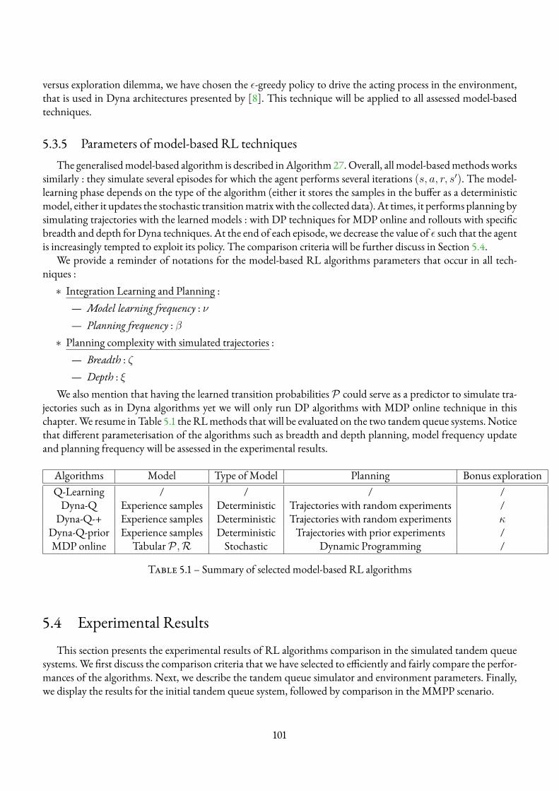
versus exploration dilemma, we have chosen the ε-greedy policy to drive the acting process in the environment,that is used in Dyna architectures presented by [8]. This technique will be applied to all assessed model-basedtechniques.

5.3.5 Parameters of model-based RL techniquesThe generalisedmodel-based algorithm is described inAlgorithm 27.Overall, all model-basedmethods works

similarly : they simulate several episodes for which the agent performs several iterations (s, a, r, s′). The model-learning phase depends on the type of the algorithm (either it stores the samples in the buffer as a deterministicmodel, either it updates the stochastic transitionmatrixwith the collected data). At times, it performs planning bysimulating trajectories with the learned models : with DP techniques for MDP online and rollouts with specificbreadth and depth forDyna techniques. At the end of each episode, we decrease the value of ε such that the agentis increasingly tempted to exploit its policy. The comparison criteria will be further discuss in Section 5.4.

We provide a reminder of notations for the model-based RL algorithms parameters that occur in all tech-niques :∗ Integration Learning and Planning :

— Model learning frequency : ν— Planning frequency : β

∗ Planning complexity with simulated trajectories :— Breadth : ζ— Depth : ξ

We also mention that having the learned transition probabilities P could serve as a predictor to simulate tra-jectories such as in Dyna algorithms yet we will only run DP algorithms with MDP online technique in thischapter.We resume in Table 5.1 the RLmethods that will be evaluated on the two tandem queue systems. Noticethat different parameterisation of the algorithms such as breadth and depth planning, model frequency updateand planning frequency will be assessed in the experimental results.

Algorithms Model Type of Model Planning Bonus explorationQ-Learning / / / /Dyna-Q Experience samples Deterministic Trajectories with random experiments /Dyna-Q-+ Experience samples Deterministic Trajectories with random experiments κ

Dyna-Q-prior Experience samples Deterministic Trajectories with prior experiments /MDP online TabularP ,R Stochastic Dynamic Programming /

Table 5.1 – Summary of selected model-based RL algorithms

5.4 Experimental ResultsThis section presents the experimental results of RL algorithms comparison in the simulated tandem queue

systems.We first discuss the comparison criteria that we have selected to efficiently and fairly compare the perfor-mances of the algorithms. Next, we describe the tandem queue simulator and environment parameters. Finally,we display the results for the initial tandem queue system, followed by comparison in the MMPP scenario.

101

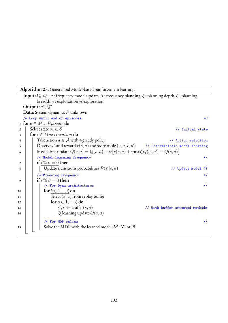
Algorithm 27:Generalised Model-based reinforcement learningInput: V0, Q0, ν : frequency model update, β : frequency planning, ξ : planning depth, ζ : planning

breadth, ε : exploitation vs explorationOutput: q∗, Q∗

Data: System dynamicsP unknown/* Loop until end of episodes */

1 for e ∈MaxEpisode do2 Select state s0 ∈ S // Initial state3 for i ∈MaxIteration do4 Take action a ∈ Awith ε-greedy policy // Action selection5 Observe s′ and reward r(s, a) and store tuple (s, a, r, s′) // Deterministic model-learning

6 Model-free updateQ(s, a) = Q(s, a) + α[r(s, a) + γmax′aQ(s′, a′)−Q(s, a)

]/* Model-learning frequency */

7 if i% ν = 0 then8 Update transitions probabilitiesP(s′|s, a) // Update model M

/* Planning frequency */9 if i% β = 0 then

/* For Dyna architectures */10 for b ∈ 1, .., ζ do11 Select (s, a) from replay buffer12 for p ∈ 1, ..., ξ do13 s′, r ← Buffer(s, a) // With buffer-oriented methods14 Q learning updateQ(s, a)

/* For MDP online */15 Solve the MDP with the learned modelM : VI or PI

102

5.4.1 Comparison Criteria between RL AlgorithmsDirectly adapting methods to compare algorithms used by practitioners is proving to have little relevance and

utility. We adopt the guidelines proposed in [34] as a guide for rigorous comparisons of reinforcement learningalgorithms. Comparisons are divided into twomain parts : comparison while learning and comparison after lear-ning on test environment.

5.4.1.1 Learning curves comparison

First, we compare different algorithms during the learning phase. Instead of only comparing the final perfor-mances of the RL methods after t timesteps in test environment, we can compare performances along learning.Indeed, performance measures while learning are represented by a learning curve. This reveal differences in speedof convergence and can provide more robust comparisons. In more detail, the learning curve will display the ave-rage discounted reward obtainedby the algorithms at the endof each learning episode.Thiswill give the evolutionof the average reward obtained and will show how fast the algorithm learns a good policy, therefore displayingthe speed of convergence. Since our problem is a cost minimisation problem, best performances will come fromalgorithm that can quickly decrease the average discounted reward.

5.4.1.2 Test policy comparison

RL algorithms should also be assessed offline. The algorithm performance after t iterations is measured as theaverage of the returns overN evaluation episodes conducted independently after training, similarly as a MonteCarlo policy evaluation. The evaluation is done implementing the policy q returned by the RL method at stept. Again, we look at the average discounted reward obtained by the plugged-in policy for comparison betweendifferent algorithms.

5.4.1.3 Comparison criteria used in our experiments

Based on literature and experimental considerations, we devised our own comparison criteria, mainly for thelearning comparison between algorithms.We express two comparisons regarding learning curves. The first one isthe average reward obtained after each learning episodes e. For this purpose, we store at the end of each episodethe average discounted reward obtained by the algorithm and plot at the end of the learning process the learningcurve that depicts the average reward over all episodes. This will show how fast the algorithms can optimise theaverage reward obtained by the updated policy, i.e. how fast the convergence is and how quickly RL algorithmscan adapt the policy in environment with changes such as Section 5.2.3.1.

After learning, we evaluate the learned policy of each algorithm in a test environment. We evaluate all policiesinMonte Carlo simulations (starting from a state s0) for 50 episodes of 10000 iterations.We finally take themeandiscounted reward obtained overall and can compare the goodness of the algorithms.

5.4.2 Simulation Environment and ParametersTo compare the list of RL algorithms, described in Section 5.3 Table 5.1, we implemented a python software

to simulate the two tandem queue systems, that serves as the environment in which the agent interacts with andcollect data.

103

5.4.2.1 Gym environment

OpenAI Gym [29] is a toolkit for developing and comparing reinforcement learning algorithms. We develo-ped a python simulator under a Gym environment. Two environments were implemented : Environment 1represents the tandem queue model and Environment 2 represents the model with MMPP. The implementa-tion of the environment class is made with two principal methods :— Reset : Reinitialise the environment with a new state s = (m1,m2, k1, k2) ;— Step(action) : Return the new state s′ and the reward r after the agent has done action a in state s by simu-

lating the uniformised probability and reward of the tandem queue model.

5.4.2.2 Cloud parameters

We ran multiple simulations on both environments. We first describe cloud simulations parameters that arecommon to all experiments. We considered three main cloud scenarios :

∗ C1 :B1 = B2 = 5,K1 = K2 = 3 , λ = 8 , µ1 = 2, µ2 = 2 ;∗ C2 :B1 = B2 = 20,K1 = K2 = 5 , λ = 15 , µ1 = 2, µ2 = 2 ;∗ C3 :B1 = B2 = 30,K1 = K2 = 8 , λ = 15 , µ1 = 2, µ2 = 2.

The cost parameters remain the same for all Cloud scenarios : {Ca = 5, Cd = 5, Cs = 10, Ch = 10, Cr =100}.

5.4.2.3 Learning parameters

The learning phase runs for 50 episodes of length 10000 iterations. One iteration corresponds to a transitionfrom state s with action a to state s′ with reward r. We collect at the end of each episode the average discountedreward obtained by the learning agent while interacting with the environment. The agent runs an epsilon-greedypolicy over thewhole learning process,with initial epsilon set to ε = 1 and epsilondecay εdec = 0.95.Wedecreaseepsilon value after each episode. The discount rate is set to γ = 0.9.

5.4.2.4 Algorithms parameters

For the first series of simulation, we provide a single set of parameters for the model-based RL algorithms.This includes frequency update of the model (formodel algorithms, frequency of planning phases and the depthof the planning phase (number of planning iterations).

Parameters for Dyna architectures For the Dyna architectures, the agent does the planning after each ite-ration, i.e. β = 1 and perform a one-step sampling for 10 samples stored in the buffer, i.e. ζ = 10 and ξ = 1.The model learning is also done after each iteration by storing the samples (s, a, r, s′) in the buffer memory, i.e.ν = 1.

Parameters for MDP online The parameters are different in the MDP online algorithm. The model lear-ning is done at the end of each episode. The agent updates the whole transition matrixP(s′|s, a) for all couples(s, a, s′) with the collected data. The model-learning frequency is thus ν = MaxIteration. For the planningpart, it is also done at the end of each episode. Once the agent have updated its MDP model with the dynamicsP , it solves the MDP with the Value Iteration algorithm to update its value function V and the policy q. Thebreadth and depth are therefore the ones of DP algorithms as displayed in Figure 3.3.

104

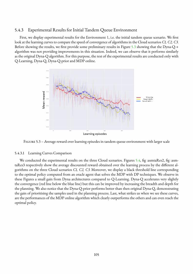
5.4.3 Experimental Results for Initial TandemQueue EnvironmentFirst, we display experimental results for the Environment 1, i.e. the initial tandem queue scenario. We first

look at the learning curves to compare the speed of convergence of algorithms in the Cloud scenarios C1, C2, C3.Before showing the results, we first provide some preliminary results in Figure 5.3 showing that the Dyna-Q-+algorithm was not providing improvements in this situation. Indeed, we can observe that it performs similarlyas the original Dyna-Q algorithm. For this purpose, the rest of the experimental results are conducted only withQ-Learning, Dyna-Q, Dyna-Q-prior andMDP online.

Figure 5.3 – Average reward over learning episodes in tandem queue environment with larger scale

5.4.3.1 Learning Curves Comparison

We conducted the experimental results on the three Cloud scenarios. Figures 5.4, fig :asmtaRes2, fig :asm-taRes3 respectively show the average discounted reward obtained over the learning process by the different al-gorithms on the three Cloud scenarios C1, C2, C3. Moreover, we display a black threshold line correspondingto the optimal policy computed from an oracle agent that solves the MDP with DP techniques. We observe inthese Figures a small gain from Dyna architectures compared to Q-Learning. Dyna-Q accelerates very slightlythe convergence (red line below the blue line) but this can be improved by increasing the breadth and depth forthe planning. We also notice that the Dyna-Q-prior performs better than then original Dyna-Q, demonstratingthe gain of prioritising the samples used in the planning process. Last, what strikes us when we see these curves,are the performances of the MDP online algorithm which clearly outperforms the others and can even reach theoptimal policy.

105

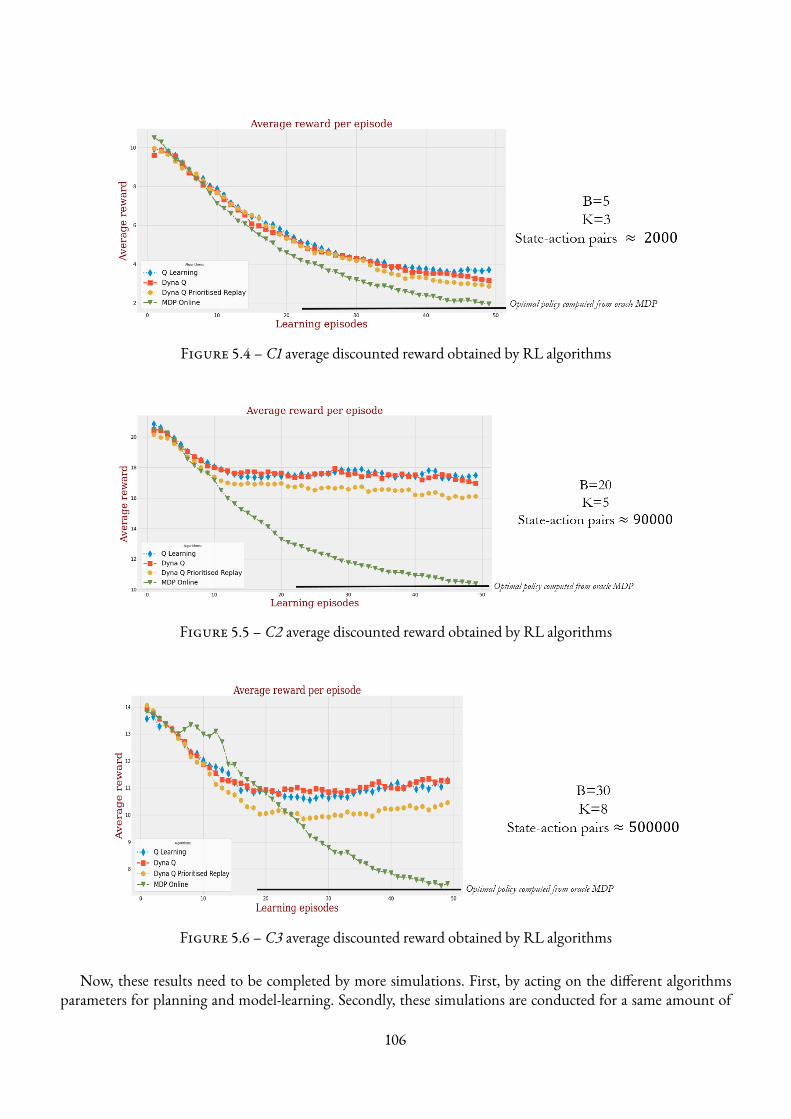
Figure 5.4 – C1 average discounted reward obtained by RL algorithms

Figure 5.5 – C2 average discounted reward obtained by RL algorithms

Figure 5.6 – C3 average discounted reward obtained by RL algorithms

Now, these results need to be completed by more simulations. First, by acting on the different algorithmsparameters for planning and model-learning. Secondly, these simulations are conducted for a same amount of

106

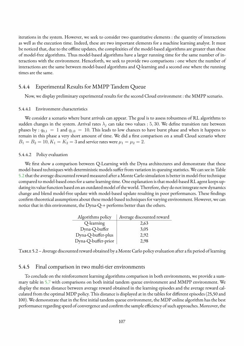
iterations in the system. However, we seek to consider two quantitative elements : the quantity of interactionsas well as the execution time. Indeed, these are two important elements for a machine learning analyst. It mustbe noticed that, due to the offline updates, the complexities of the model-based algorithms are greater than theseof model-free algorithms. Thus model-based algorithms have a larger running time for the same number of in-teractions with the environment. Henceforth, we seek to provide two comparisons : one where the number ofinteractions are the same between model-based algorithms and Q-learning and a second one where the runningtimes are the same.

5.4.4 Experimental Results for MMPP TandemQueueNow, we display preliminary experimental results for the second Cloud environment : the MMPP scenario.

5.4.4.1 Environment characteristics

We consider a scenario where burst arrivals can appear. The goal is to assess robustness of RL algorithms tosudden changes in the system. Arrival rates λj can take two values : 5, 30. We define transition rate betweenphases by : q0,1 = 1 and q1,0 = 10. This leads to low chances to have burst phase and when it happens toremain in this phase a very short amount of time. We did a first comparison on a small Cloud scenario whereB1 = B2 = 10, K1 = K2 = 3 and service rates were µ1 = µ2 = 2.

5.4.4.2 Policy evaluation

We first show a comparison between Q-Learning with the Dyna architectures and demonstrate that thesemodel-based techniques with deterministicmodels suffer from variation in queuing statistics.We can see in Table5.2 that the average discounted rewardmeasured after aMonte Carlo simulation is better inmodel-free techniquecompared tomodel-based ones for a same learning time.One explanation is thatmodel-basedRL agent keeps up-dating its value functionbased on anoutdatedmodel of theworld.Therefore, they donot integrate newdynamicschange and blend model-free update with model-based update resulting in poor performances. These findingsconfirm theoretical assumptions about thesemodel-based techniques for varying environment. However, we cannotice that in this environment, the Dyna-Q-+ performs better than the others.

Algorithms policy Average discounted rewardQ-learning 2,63

Dyna-Q-buffer 3,05Dyna-Q-buffer-plus 2,92Dyna-Q-buffer-prior 2,98

Table 5.2 –Average discounted reward obtained by aMonteCarlo policy evaluation after a fix period of learning

5.4.5 Final comparison in two multi-tier environmentsTo conclude on the reinforcement learning algorithms comparison in both environments, we provide a sum-

mary table in 5.7 with comparisons on both initial tandem queue environment and MMPP environment. Wedisplay the mean distance between average reward obtained in the learning episodes and the average reward cal-culated from the optimalMDP policy. This distance is displayed at in the tables for different episodes (25,50 and100).We demonstrate that in the first initial tandem queue environment, theMDP online algorithm has the bestperformance regarding speed of convergence and confirm the sample efficiency of such approaches.Moreover, the

107

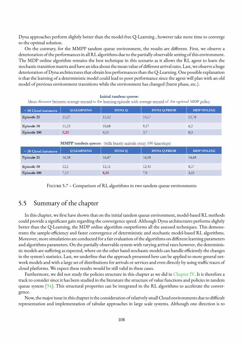
Dyna approaches perform slightly better than the model-free Q-Learning , however take more time to convergeto the optimal solution.

On the contrary, for the MMPP tandem queue environment, the results are different. First, we observe adeterioration of the performances in all RL algorithms due to the partially observable setting of this environment.The MDP online algorithm remains the best technique in this scenario as it allows the RL agent to learn thestochastic transitionmatrix andhave an idea about themean value of different arrival rates. Last,weobserve a hugedeterioration ofDyna architectures that obtain less performances than theQ-Learning.One possible explanationis that the learning of a deterministic model could lead to poor performance since the agent will plan with an oldmodel of previous environment transitions while the environment has changed (burst phase, etc.).

Figure 5.7 – Comparison of RL algorithms in two tandem queue environments

5.5 Summary of the chapterIn this chapter, we first have shown that on the initial tandem queue environment, model-based RLmethods

could provide a significant gain regarding the convergence speed. Although Dyna architectures performs slightlybetter than the Q-Learning, the MDP online algorithm outperforms all the assessed techniques. This demons-trates the sample-efficiency and faster convergence of deterministic and stochastic model-based RL algorithms.Moreover,more simulations are conducted for a fair evaluation of the algorithms ondifferent learning parametersand algorithms parameters. On the partially observable systemwith varying arrival rates however, the determinis-tic models are suffering as expected, where on the other hand stochastic models can handle efficiently the changesin the system’s statistics. Last, we underline that the approach presented here can be applied to more general net-work models and with a large set of distributions for arrivals or services and even directly by using traffic traces ofcloud platforms. We expect these results would be still valid in these cases.

Furthermore, we did not study the policies structure in this chapter as we did in Chapter IV. It is therefore atrack to consider since it has been studied in the literature the structure of value functions and policies in tandemqueue system [94]. This structural properties can be integrated in the RL algorithms to accelerate the conver-gence.

Now, themajor issue in this chapter is the consideration of relatively small Cloud environments due to difficultrepresentation and implementation of tabular approaches in large scale systems. Although one direction is to

108

consider approximation approaches such as described in Section 5.1, we decided next to investigate structuralapproaches and to assess if providingmore knowledge about the environment to the agent could help to representmore compactly theworldmodel and also could help for convergence acceleration.These approaches are exploredin the following chapters with Factored RL Chapter VI and Causal RL Chapter VII.

109

PART III

MODEL-BASEDREINFORCEMENTLEARNINGWITHRELATIONAL

STRUCTURE BETWEEN ENVIRONMENTVARIABLES

110

CHAPTER 6

FACTOREDREINFORCEMENT LEARNING FORMULTI-TIERNETWORK

The contributions of this chapter have been published in [140] :∗ Thomas Tournaire, Yue Jin, Armen Aghasaryan, Hind Castel-Taleb, Emmanuel Hyon. Factored Reinfor-cement Learning for Auto-scaling in TandemQueues. InNetwork and Service Management in the Era ofCloudification, Softwarization and Artificial Intelligence (NOMS 22), 2022

In the precedent chapters, we only considered tabular representations of dynamics and reward models whichmay be impractical in large scale environments with very high size state and action spaces. As we have seen at thebeginning of this work, the factored MDP framework ought to represent more compactly the modelM of theworld by integrating the relations between environment variables. In environments which have specific relationsbetween state variables, it could be highly beneficial to use this representation to accelerate the convergence andthe ease of implementation.

This chapters proposes FMDP online, a factored RL algorithm that can overcome convergence issues byexpressing the problem in a compact form. Indeed, all the solutions described in theMDP framework of chap IVand chap V, whether for planning or reinforcement learning with models, all share a common drawback : theyare not adapted to the resolution of large problems. The use of unstructured representations such as tables fordynamics and value function requires an explicit enumeration of the set of all the possible states of the problemto represent the functions necessary to solve it.

The factored approach provides the learning agent with the relational structure of the environment, here withDynamic Bayesian Networks (DBN). Indeed, we believe that in distributed network environments such as 5Gslicing architectures, queuing networks or multi-tier infrastructures presented here with the tandem queue mo-del, there exist local dependencies between physical nodes. Events in a physical node have direct impacts onlyon its neighbours and affect other nodes indirectly in most cases. In this context Factored MDP [26] frame-work takes advantage of local dependencies structure in the environment, accelerates convergence and overcomesthe so-called ’curse of dimensionality’ in MDP solutions. We use the Factored MDP framework to model theauto-scaling problem in the tandem queue with two nodes, described in section 5.2.1. The very few number ofapplications with factored solutions in the literature call for further research in this topic and for comparisonwith existingmodel-free andmodel-based algorithms. To the best of our knowledge, we have not seen works thatapply factored RL approaches on networking systems and this is why we wanted to investigate such approach ina feasible environment.

111

Contributions of this chapter are as follows :∗ Proposal of FMDP online algorithm;∗ FactoredMDPmodel for the tandem queue environment ;∗ Comparison of FMDP online with state of the art algorithms on the tandem queue model.

6.1 BackgroundWe first providemore details about the FactoredMarkovDecisionProcess (FMDP) framework thatwas briefly

introduced in Chapter III, by providing mathematical formalism and state of the art algorithms.

6.1.1 Coffee Robot Example : Illustration for the factored frameworkTo illustrate the factored representational methodology, we will use the Co�ee Robot example of a feature-

based, stochastic, sequential decision problem, following the work of [26]. In this example, a robot, aka the lear-ning agent, must go to a coffee shop to buy a cup of coffee for its owner who is located at its office. When it israining, it must get an umbrella to stay dry when going to the shop. The state of the system is composed of sixbinary variables si whereDom(si) = {0, 1} (corresponding respectively to False and True). These variables are :∗ sH : Has the owner a coffee?∗ sC : Has the robot a coffee?∗ sW : Is the robot wet?∗ sR : Is it raining?∗ sU : Has the robot an umbrella?∗ sO : Is the robot in the office?

This problem being composed of 6 binary variables, there is 26 = 64 possible states. In this problem, four actionsare available to the robot :

∗ Go : Move to the other location;∗ BuyC : Buy a coffee (only available in the coffee shop) ;∗ DelC : Deliver coffee to the owner (only possible in the office and if the robot has coffee) ;∗ GetU : Get an umbrella (only in the office).

Actions can be noisy to represent stochastic problems. For instance, when the robot gives the coffee, its ownerwill get his coffee only with a given probability (the cup may fall). Thus, when the action DelC is executed in thestate s = (sC = 0, sH = 1, sW = 0, sR = 1, sU = 0, sO = 1) (the robot is in the office and the owner doesnot have a coffee), the transition function of the problem defines :— P((sC = 1, sH = 1, sW = 0, sR = 1, sU = 0, sO = 1)|s,DelC) = 0.8 ;— P((sC = 0, sH = 1, sW = 0, sR = 1, sU = 0, sO = 1)|s,DelC) = 0.2.Otherwise all remains deterministic. Finally, for the reward function, the robot gets a reward of 0.9when the

owner has a coffee (0when it does not) and 0.1when it is dry (and 0when the robot is wet). The reward the robotobtains when the owner gets a coffee is larger than the reward obtained when the robot is dry so as to specify thatthe task of getting a coffee has a higher priority than the constraint of staying dry.

112

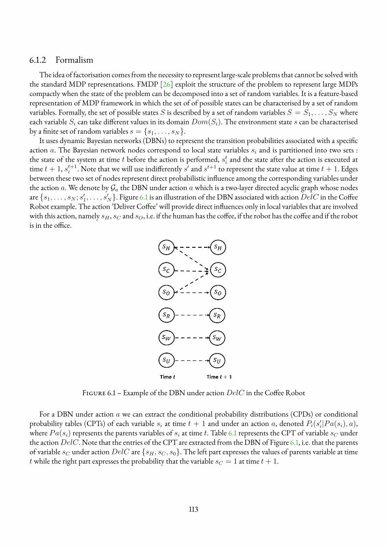
6.1.2 FormalismThe idea of factorisation comes from the necessity to represent large-scale problems that cannot be solvedwith

the standard MDP representations. FMDP [26] exploit the structure of the problem to represent large MDPscompactly when the state of the problem can be decomposed into a set of random variables. It is a feature-basedrepresentation of MDP framework in which the set of of possible states can be characterised by a set of randomvariables. Formally, the set of possible states S is described by a set of random variables S = S1, . . . , SN whereeach variable Si can take different values in its domainDom(Si). The environment state s can be characterisedby a finite set of random variables s = {s1, . . . , sN}.

It uses dynamic Bayesian networks (DBNs) to represent the transition probabilities associated with a specificaction a. The Bayesian network nodes correspond to local state variables si and is partitioned into two sets :the state of the system at time t before the action is performed, sti and the state after the action is executed attime t + 1, st+1

i . Note that we will use indifferently s′ and st+1 to represent the state value at time t + 1. Edgesbetween these two set of nodes represent direct probabilistic influence among the corresponding variables underthe action a. We denote by Ga the DBN under action a which is a two-layer directed acyclic graph whose nodesare {s1, . . . , sN ; s′1, . . . , s

′N}. Figure 6.1 is an illustration of the DBN associated with actionDelC in the Coffee

Robot example. The action ’Deliver Coffee’ will provide direct influences only in local variables that are involvedwith this action, namely sH , sC and sO, i.e. if the human has the coffee, if the robot has the coffee and if the robotis in the office.

Figure 6.1 – Example of the DBN under actionDelC in the Coffee Robot

For a DBN under action a we can extract the conditional probability distributions (CPDs) or conditionalprobability tables (CPTs) of each variable si at time t + 1 and under an action a, denoted Pi(s′i|Pa(si), a),where Pa(si) represents the parents variables of si at time t. Table 6.1 represents the CPT of variable sC underthe actionDelC . Note that the entries of the CPT are extracted from the DBN of Figure 6.1, i.e. that the parentsof variable sC under actionDelC are {sH , sC , s0}. The left part expresses the values of parents variable at timetwhile the right part expresses the probability that the variable sC = 1 at time t+ 1.

113

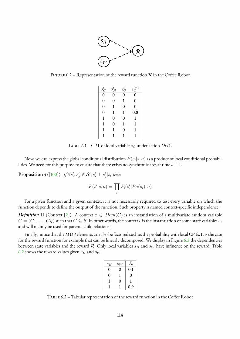
Figure 6.2 – Representation of the reward functionR in the Coffee Robot

stC stH stO st+1C

0 0 0 00 0 1 00 1 0 00 1 1 0.81 0 0 11 0 1 11 1 0 11 1 1 1

Table 6.1 – CPT of local variable sC under actionDelC

Now, we can express the global conditional distribution P (s′|s, a) as a product of local conditional probabi-lities. We need for this purpose to ensure that there exists no synchronic arcs at time t+ 1.

Proposition 4 ([100]). If ∀s′i, s′j ∈ S ′, s′i ⊥ s′j|s, then

P (s′|s, a) =∏i

Pi(s′i|Pa(si), a)

For a given function and a given context, it is not necessarily required to test every variable on which thefunction depends to define the output of the function. Such property is named context-specific independence.Definition 11 (Context [2]). A context c ∈ Dom(C) is an instantiation of a multivariate random variableC = (C0, . . . , CK) such thatC ⊆ S. In other words, the context c is the instantiation of some state variables siand will mainly be used for parents-child relations.

Finally, notice that theMDP elements can also be factored such as the probabilitywith local CPTs. It is the casefor the reward function for example that can be linearly decomposed. We display in Figure 6.2 the dependenciesbetween state variables and the rewardR. Only local variables sH and sW have influence on the reward. Table6.2 shows the reward values given sH and sW .

sH sW R0 0 0.10 1 01 0 11 1 0.9

Table 6.2 – Tabular representation of the reward function in the Coffee Robot

114

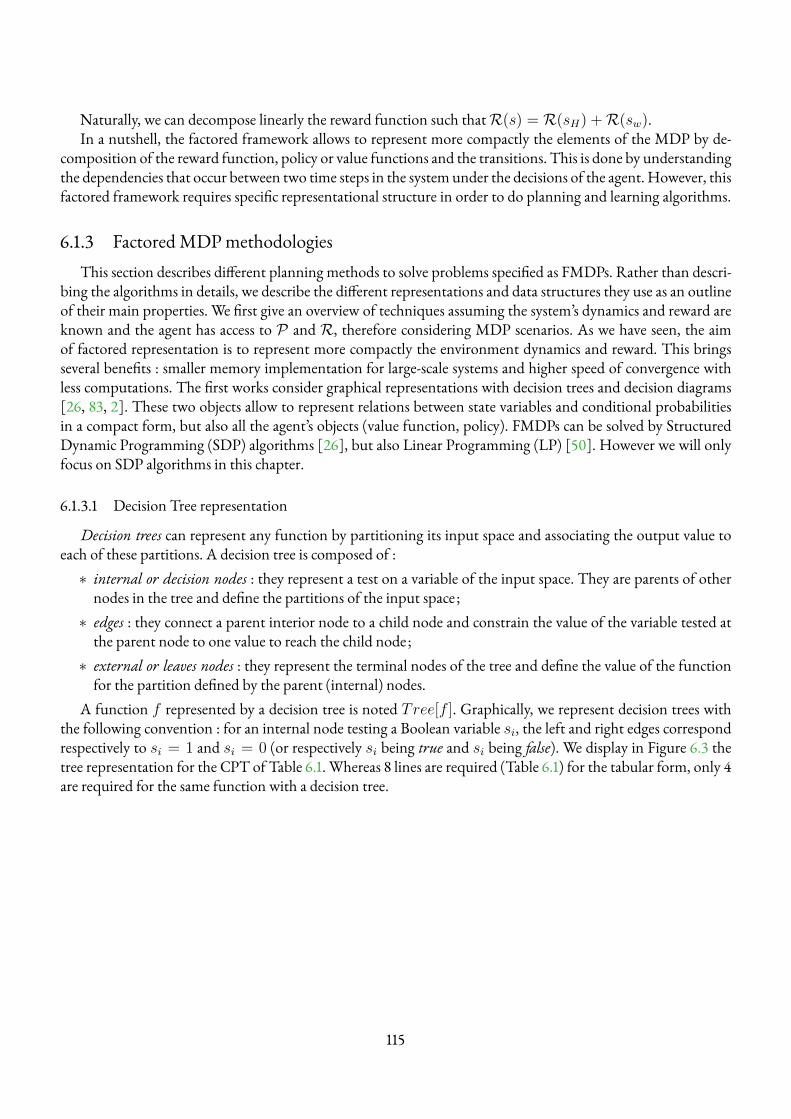
Naturally, we can decompose linearly the reward function such thatR(s) = R(sH) +R(sw).In a nutshell, the factored framework allows to represent more compactly the elements of the MDP by de-

composition of the reward function, policy or value functions and the transitions. This is done by understandingthe dependencies that occur between two time steps in the system under the decisions of the agent.However, thisfactored framework requires specific representational structure in order to do planning and learning algorithms.

6.1.3 FactoredMDPmethodologiesThis section describes different planning methods to solve problems specified as FMDPs. Rather than descri-

bing the algorithms in details, we describe the different representations and data structures they use as an outlineof their main properties. We first give an overview of techniques assuming the system’s dynamics and reward areknown and the agent has access to P and R, therefore considering MDP scenarios. As we have seen, the aimof factored representation is to represent more compactly the environment dynamics and reward. This bringsseveral benefits : smaller memory implementation for large-scale systems and higher speed of convergence withless computations. The first works consider graphical representations with decision trees and decision diagrams[26, 83, 2]. These two objects allow to represent relations between state variables and conditional probabilitiesin a compact form, but also all the agent’s objects (value function, policy). FMDPs can be solved by StructuredDynamic Programming (SDP) algorithms [26], but also Linear Programming (LP) [50]. However we will onlyfocus on SDP algorithms in this chapter.

6.1.3.1 Decision Tree representation

Decision trees can represent any function by partitioning its input space and associating the output value toeach of these partitions. A decision tree is composed of :∗ internal or decision nodes : they represent a test on a variable of the input space. They are parents of othernodes in the tree and define the partitions of the input space ;∗ edges : they connect a parent interior node to a child node and constrain the value of the variable tested atthe parent node to one value to reach the child node;∗ external or leaves nodes : they represent the terminal nodes of the tree and define the value of the functionfor the partition defined by the parent (internal) nodes.

A function f represented by a decision tree is noted Tree[f ]. Graphically, we represent decision trees withthe following convention : for an internal node testing a Boolean variable si, the left and right edges correspondrespectively to si = 1 and si = 0 (or respectively si being true and si being false). We display in Figure 6.3 thetree representation for the CPT of Table 6.1. Whereas 8 lines are required (Table 6.1) for the tabular form, only 4are required for the same function with a decision tree.

115

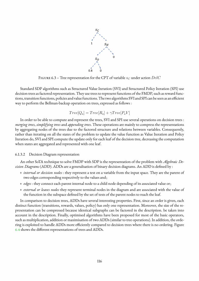
Figure 6.3 – Tree representation for the CPT of variable sC under actionDelC

Standard SDP algorithms such as Structured Value Iteration (SVI) and Structured Policy Iteration (SPI) usedecision trees as factored representation. They use trees to represent functions of the FMDP, such as reward func-tions, transition functions, policies andvalue functions.The twoalgorithmsSVI andSPI canbe seen as an efficientway to perform the Bellman-backup operation on trees, expressed as follows :

Tree[Qa] = Tree[Ra] + γTree[PaV ]

In order to be able to compute and represent the trees, SVI and SPI use several operations on decision trees :merging trees, simplifying trees and appending trees. These operations are mainly to compress the representationsby aggregating nodes of the trees due to the factored structure and relations between variables. Consequently,rather than iterating on all the states of the problem to update the value function as Value Iteration and PolicyIteration do, SVI and SPI compute the update only for each leaf of the decision tree, decreasing the computationwhen states are aggregated and represented with one leaf.

6.1.3.2 Decision Diagram representation

An other SoTA technique to solve FMDP with SDP is the representation of the problem withAlgebraic De-cision Diagrams (ADD). ADDs are a generalisation of binary decision diagrams. An ADD is defined by :∗ internal or decision nodes : they represent a test on a variable from the input space. They are the parent oftwo edges corresponding respectively to the values and;∗ edges : they connect each parent internal node to a child node depending of its associated value or ;∗ external or leaves nodes they represent terminal nodes in the diagram and are associated with the value ofthe function in the subspace defined by the set of tests of the parent nodes to reach the leaf.

In comparison to decision trees, ADDs have several interesting properties. First, since an order is given, eachdistinct function (transitions, rewards, values, policy) has only one representation. Moreover, the size of the re-presentation can be compressed because identical subgraphs can be factored in the description. be taken intoaccount in the description. Finally, optimised algorithms have been proposed for most of the basic operators,such asmultiplication, addition ormaximisation of twoADDs (similar to tree operations). In addition, the orde-ring is exploited to handle ADDs more efficiently compared to decision trees where there is no ordering. Figure6.4 shows the different representations of trees and ADDs.

116

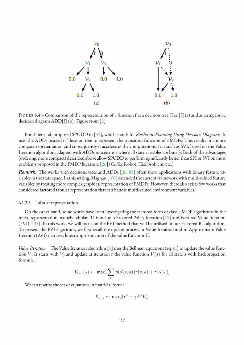
Figure 6.4 – Comparison of the representation of a function f as a decision tree Tree [f] (a) and as an algebraicdecision diagram ADD[f] (b) ; Figure from [2]

Boutlilier et al. proposed SPUDD in [59], which stands for Stochastic Planning Using Decision Diagrams. Ituses the ADDs instead of decision tree to represent the transition function of FMDPs. This results in a morecompact representation and consequently it accelerates the computations. It is such as SVI, based on the ValueIteration algorithm, adapted with ADDs in scenarios where all state variables are binary. Both of the advantages(ordering,more compact) described above allow SPUDD to perform significantly better than SPI or SVI onmostproblems proposed in the FMDP literature [26] (Coffee Robot, Taxi problem, etc.).Remark. The works with decisions trees and ADDs [26, 83] often show applications with binary feature va-riables in the state space. In this setting,Magnan [100] extended the current frameworkwithmulti-valued featurevariables by treatingmore complex graphical representation of FMDPs.However, there also exists fewworks thatconsidered factored tabular representation that can handle multi-valued environment variables.

6.1.3.3 Tabular representation

On the other hand, some works have been investigating the factored form of classic MDP algorithms in theinitial representation, namely tabular. This includes Factored Policy Iteration [79] and Factored Value Iteration(FVI) [135]. In this work, we will focus on the FVI method that will be utilised in our Factored RL algorithm.To present the FVI algorithm, we first recall the update process in Value Iteration and in Approximate ValueIteration (AVI) that uses linear approximation of the value function V .

Value Iteration The Value Iteration algorithm [5] uses the Bellman equations (eq 3.1) to update the value func-tion V . It starts with V0 and update at iteration t the value function V (s) for all state s with backprojectionformula :

Vt+1(s)← maxa∑s′

p(s′|s, a) [r(s, a) + γVt(s′)]

We can rewrite the set of equations in matricial form :

Vt+1 ← maxa(ra + γP aVt)

117

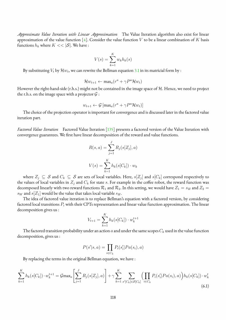
Approximate Value Iteration with Linear Approximation The Value Iteration algorithm also exist for linearapproximation of the value function [4]. Consider the value function V to be a linear combination ofK basisfunctions hk whereK << |S|. We have :

V (s) =K∑k=1

wkhk(s)

By substituting Vt byHwt, we can rewrite the Bellman equation 3.1 in its matricial form by :

Hwt+1 ← maxa(ra + γP aHwt)However the right-hand-side (r.h.s.) might not be contained in the image space ofH. Hence, we need to projectthe r.h.s. on the image space with a projector G :

wt+1 ← G [maxa(ra + γP aHwt)]The choice of the projection operator is important for convergence and is discussed later in the factored value

iteration part.

Factored Value Iteration Factored Value Iteration [135] presents a factored version of the Value Iteration withconvergence guarantees. We first have linear decomposition of the reward and value functions.

R(s, a) =J∑j=1

Rj(s[Zj], a)

V (s) =K∑k=1

hk(s[Ck]) · wk

where Zj ⊆ S and Ck ⊆ S are sets of local variables. Here, s[Zj] and s[Ck] correspond respectively tothe values of local variables in Zj and Ck for state s. For example in the coffee robot, the reward function wasdecomposed linearly with two reward functionsR1 andR2. In this setting, we would have Z1 = sH and Z2 =sW and s[Z1] would be the value that takes local variable sH .

The idea of factored value iteration is to replace Bellman’s equation with a factored version, by consideringfactored local transitions Pi with their CPTs representation and linear value function approximation. The lineardecomposition gives us :

Vt+1 =K∑k=1

hk(s[Ck]) · wt+1k

The factored transition probability under an actiona and under the same scopesCk used in the value functiondecomposition, gives us :

P (s′|s, a) =∏i∈Ck

Pi(s′i|Pa(si), a)

By replacing the terms in the original Bellman equation, we have :

K∑k=1

hk(s[Ck]) ·wt+1k = Gmaxa

[J∑j=1

Rj(s[Zj], a)

]+γ

K∑k=1

∑s′[Ck]∈S[Ck]

(∏i∈Ck

Pi(s′i|Pa(si), a)

)hk(s[Ck]) ·wtk

(6.1)

118

We can observe in equation 6.1 that the update complexity is reduced compared to the original Bellman equa-tion 3.1 since we do less calculations by considering the factored form of transitions. By considering the backpro-jection matrix B such that :

Bas,k =∑

s′[Ck]∈S[Ck]

(∏i∈Ck

Pi(s′i|Pa(si), a)

)hk(s

′[Ck])

we have in matricial computation the update of the value function’s weights by :

wt+1 = Gmaxa[ra + γBawt

]where G is the matrix form of the projection operator G.Overall, they show that their algorithm is only polynomial in the number of basis functions k, which de-

monstrates a huge gain compared to originalMDPValue Iteration. Also, the authors [135] propose in their worka sampling method to work on a subset of the original state space S ⊆ S where |S| = poly(N). Algorithm 28displays the FVI algorithm.

Algorithm 28: Factored Value IterationInput: Basis functionsHi,G projector, V 0 = Hw0, q0, ξ accuracyOutput: q∗, V ∗

Data: Statistics and DBNs known1 N1 number of samples // Sampling method

2 S uniform randomN1-elements subset of S3 Create H and G4 Create Ba = ˆP aH and ra for all actions a ∈ A5 w0 = 0, t = 06 repeat7 wt+1 = Gmaxa

[ra + γBawt

]8 ∆t = ||wt+1 − wt||9 t← t+ 1

10 until ∆t ≤ ξ11 returnwt, V t, qt

6.1.4 Factored Reinforcement LearningSo far, we have provided an overview of factored techniques to solveMarkovDecision Process scenarios where

the agent was provided the true environment model. These methods are inspired by DP algorithms often usedfor MDP resolutions. Several works have also proposed factored solutions in the RL paradigm where the agenthas missing knowledge and needs to learn from data the model of the world to perform planning. We find inthese proposal the same characteristics as in the model-based RL domain, namely, the learning and planningin the factored framework. Factored Reinforcement Learning (FRL) [73, 83] is a model-based ReinforcementLearning approach to FMDPswhere the transition and reward functions of the problem are learned. First, it usesthe methods of Supervised Learning to construct the factored representation of the environment. In parallel,planning algorithms can use this representation to build the policy.

The FRL algorithms are mainly inspired byDyna architectures (deterministic models) andMDP online tech-niques (stochastic models). Among these methods the structural knowledge is an hypothesis that can be assumed

119

or not. Therefore, someworks [73, 83] require to learn only the statistics because the agent already knows how theenvironment variables influence each other. In other words, the learning agent is provided the relational structureof the environment but does not know the statistics. Nevertheless, other researchers [35] have tempted to consi-der more complex scenarios where the agent should also learn the relations between variables from the collecteddata.

6.1.4.1 Factored Dyna architectures : SDYNA

Structured-Dyna (SDYNA) framework proposed byDegris et al. [35], is a structured version of theDYNAar-chitecture. SDYNA integrates incremental planning algorithms based on FMDPs with supervised learning tech-niques building structured representations of the problem. It uses the decision tree representation. The innerloop of SDYNA is decomposed into three phases :∗ Acting : choosing an action according to the current policy, including some exploration;∗ Model-Learning : updating themodel of the transition and reward functions of the FMDP from (s, a, r, s′)observations ;∗ Planning : updating the value functionTree[V ] and policyTree[q] using one iteration of SDP algorithms.

6.1.4.2 FactoredMDP online

It has also been proposed solutions for stochastic models methods. For model-based Reinforcement Lear-ning techniques, Kearns and al. present in [73] a factored implementation of the E3 MDP-online algorithm,called DBN-E3. The authors proposed a provably efficient and near-optimal algorithm that generalises the E3technique. In their work, they assume that they are given both an algorithm for approximate planning, and thegraphical structure (but not the parameters) of the DBN. Unlike the original E3 algorithm, this factored versionof E3 exploits the DBN structure to achieve a running time that scales polynomially in the number of parametersof the DBN, which may be exponentially smaller than the number of global states.

Guestrin et al. [51] also proposed a factored version for the R-max algorithm, called Factored R-max. In theirwork, Guestrin et al. address a significant shortcoming of Factored E3 : namely that it requires an oracle plannerthat cannot be feasibly implemented. They propose an alternative approach that uses a practical approximateplanner and approximate linear programming. Furthermore, they develop an exploration strategy that is targetedtoward improving the performance of the linear programming algorithm, rather than an oracle planner. Thisleads to a simple exploration strategy that visits the relevant states for the LP solution, and achieves logarithmicsample efficiency in the size of the problem description. Moreover, they show in experimental results that theirproposal performs better.

Finnaly, Strehl et al. [131] have studied the optimality and performances of both factored E3 and factoredRmax. They have shown that factored Rmax was performing near-optimally on all but a number of timestepsthat is polynomial in the size of the compact representation,which is often exponentially smaller than the numberof states and showed the equivalence with the result obtained by Kearns and Koller [73] for their DBN-E3 algo-rithm. Moreover they proposed a new algorithm inspired from the two above, Factored IE that uses the IntervalEstimation approach to exploration and can be expected to outperform factored Rmax on most domains.

6.1.4.3 Learning the structure - SPITI

Finally, some works have considered cases where the learning agent was not provided the structure of theenvironment (e.g.DBN).Degris et al. [35] have extended the SDYNAalgorithm in scenarioswhere the agent alsoneeds to learn the structure of the FMDPandderived the SPITI. SPITI is a particular instance of SDYNAusing ε-greedy as exploration method, the Incremental Tree Induction (ITI) algorithm to learn the model of transitions

120

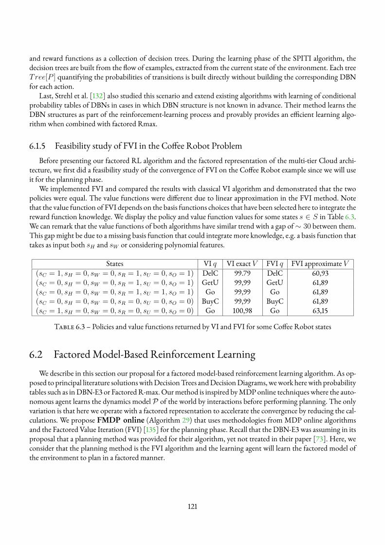
and reward functions as a collection of decision trees. During the learning phase of the SPITI algorithm, thedecision trees are built from the flow of examples, extracted from the current state of the environment. Each treeTree[P ] quantifying the probabilities of transitions is built directly without building the corresponding DBNfor each action.

Last, Strehl et al. [132] also studied this scenario and extend existing algorithms with learning of conditionalprobability tables of DBNs in cases in which DBN structure is not known in advance. Their method learns theDBN structures as part of the reinforcement-learning process and provably provides an efficient learning algo-rithm when combined with factored Rmax.

6.1.5 Feasibility study of FVI in the Coffee Robot ProblemBefore presenting our factored RL algorithm and the factored representation of the multi-tier Cloud archi-

tecture, we first did a feasibility study of the convergence of FVI on the Coffee Robot example since we will useit for the planning phase.

We implemented FVI and compared the results with classical VI algorithm and demonstrated that the twopolicies were equal. The value functions were different due to linear approximation in the FVI method. Notethat the value function of FVI depends on the basis functions choices that have been selected here to integrate thereward function knowledge. We display the policy and value function values for some states s ∈ S in Table 6.3.We can remark that the value functions of both algorithms have similar trend with a gap of∼ 30 between them.This gapmight be due to a missing basis function that could integrate more knowledge, e.g. a basis function thattakes as input both sH and sW or considering polynomial features.

States VI q VI exact V FVI q FVI approximate V(sC = 1, sH = 0, sW = 0, sR = 1, sU = 0, sO = 1) DelC 99.79 DelC 60,93(sC = 0, sH = 0, sW = 0, sR = 1, sU = 0, sO = 1) GetU 99,99 GetU 61,89(sC = 0, sH = 0, sW = 0, sR = 1, sU = 1, sO = 1) Go 99,99 Go 61,89(sC = 0, sH = 0, sW = 0, sR = 0, sU = 0, sO = 0) BuyC 99,99 BuyC 61,89(sC = 1, sH = 0, sW = 0, sR = 0, sU = 0, sO = 0) Go 100,98 Go 63,15

Table 6.3 – Policies and value functions returned by VI and FVI for some Coffee Robot states

6.2 FactoredModel-Based Reinforcement LearningWe describe in this section our proposal for a factored model-based reinforcement learning algorithm. As op-

posed to principal literature solutionswithDecisionTrees andDecisionDiagrams,wework herewith probabilitytables such as inDBN-E3 or FactoredR-max.Ourmethod is inspired byMDPonline techniques where the auto-nomous agent learns the dynamics model P of the world by interactions before performing planning. The onlyvariation is that here we operate with a factored representation to accelerate the convergence by reducing the cal-culations. We propose FMDP online (Algorithm 29) that uses methodologies from MDP online algorithmsand the Factored Value Iteration (FVI) [135] for the planning phase. Recall that the DBN-E3 was assuming in itsproposal that a planning method was provided for their algorithm, yet not treated in their paper [73]. Here, weconsider that the planning method is the FVI algorithm and the learning agent will learn the factored model ofthe environment to plan in a factored manner.

121

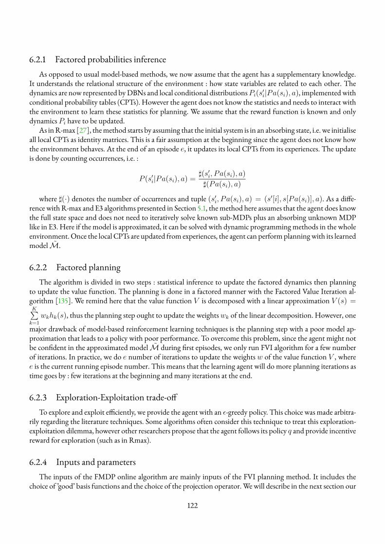
6.2.1 Factored probabilities inferenceAs opposed to usual model-based methods, we now assume that the agent has a supplementary knowledge.

It understands the relational structure of the environment : how state variables are related to each other. Thedynamics are now represented byDBNs and local conditional distributionsPi(s′i|Pa(si), a), implementedwithconditional probability tables (CPTs). However the agent does not know the statistics and needs to interact withthe environment to learn these statistics for planning. We assume that the reward function is known and onlydynamics Pi have to be updated.

As inR-max [27], themethod starts by assuming that the initial system is in an absorbing state, i.e. we initialiseall local CPTs as identity matrices. This is a fair assumption at the beginning since the agent does not know howthe environment behaves. At the end of an episode e, it updates its local CPTs from its experiences. The updateis done by counting occurrences, i.e. :

P (s′i|Pa(si), a) =](s′i, Pa(si), a)

](Pa(si), a)

where ](·) denotes the number of occurrences and tuple (s′i, Pa(si), a) = (s′[i], s[Pa(si)], a). As a diffe-rence with R-max and E3 algorithms presented in Section 5.1, themethod here assumes that the agent does knowthe full state space and does not need to iteratively solve known sub-MDPs plus an absorbing unknown MDPlike in E3. Here if the model is approximated, it can be solved with dynamic programming methods in the wholeenvironment.Once the local CPTs are updated from experiences, the agent can performplanningwith its learnedmodel M.

6.2.2 Factored planningThe algorithm is divided in two steps : statistical inference to update the factored dynamics then planning

to update the value function. The planning is done in a factored manner with the Factored Value Iteration al-gorithm [135]. We remind here that the value function V is decomposed with a linear approximation V (s) =K∑k=1

wkhk(s), thus the planning step ought to update the weightswk of the linear decomposition. However, one

major drawback of model-based reinforcement learning techniques is the planning step with a poor model ap-proximation that leads to a policy with poor performance. To overcome this problem, since the agent might notbe confident in the approximated model M during first episodes, we only run FVI algorithm for a few numberof iterations. In practice, we do e number of iterations to update the weights w of the value function V , wheree is the current running episode number. This means that the learning agent will do more planning iterations astime goes by : few iterations at the beginning and many iterations at the end.

6.2.3 Exploration-Exploitation trade-offTo explore and exploit efficiently, we provide the agent with an ε-greedy policy. This choice was made arbitra-

rily regarding the literature techniques. Some algorithms often consider this technique to treat this exploration-exploitation dilemma, however other researchers propose that the agent follows its policy q and provide incentivereward for exploration (such as in Rmax).

6.2.4 Inputs and parametersThe inputs of the FMDP online algorithm are mainly inputs of the FVI planning method. It includes the

choice of ’good’ basis functions and the choice of the projection operator.Wewill describe in the next section our

122

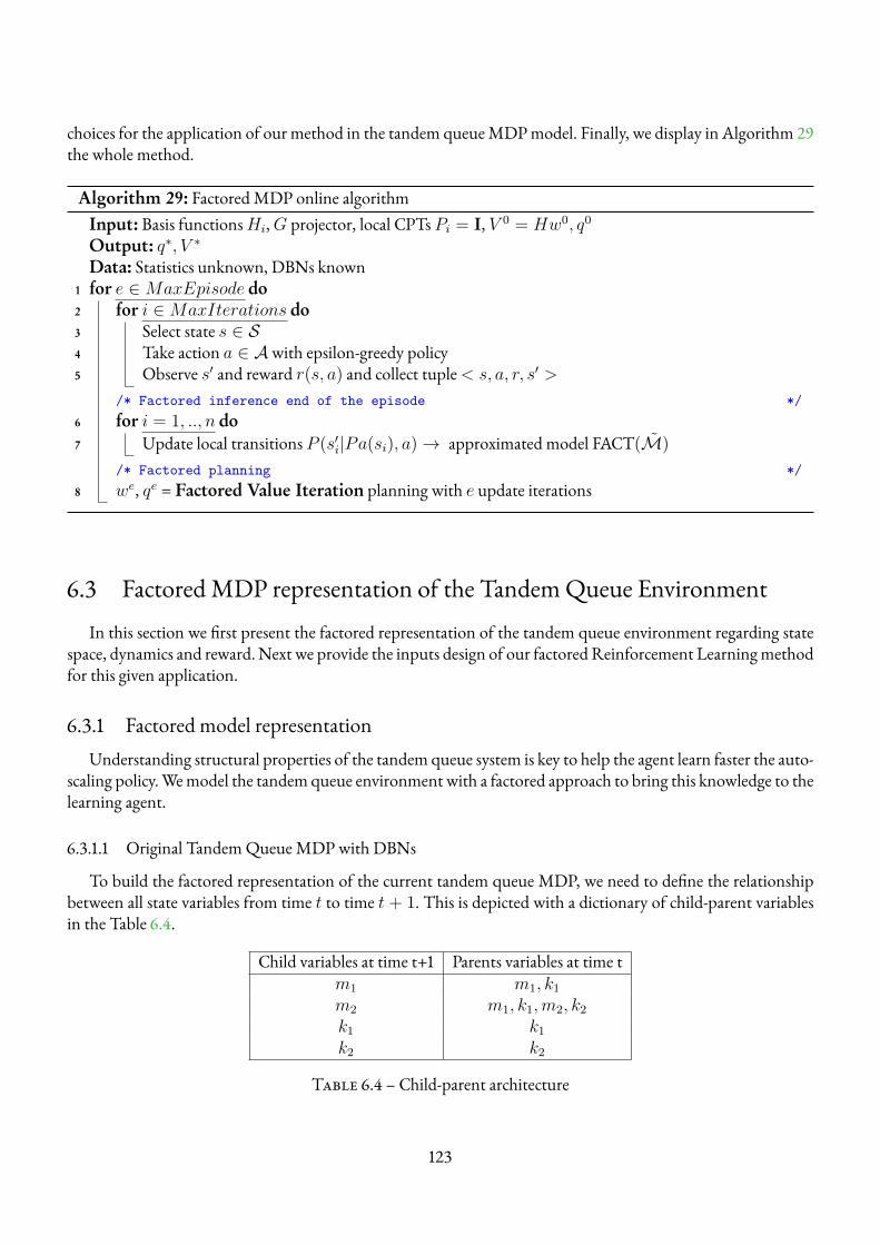
choices for the application of our method in the tandem queueMDPmodel. Finally, we display in Algorithm 29the whole method.

Algorithm 29: FactoredMDP online algorithmInput: Basis functionsHi,G projector, local CPTs Pi = I, V 0 = Hw0, q0

Output: q∗, V ∗

Data: Statistics unknown, DBNs known1 for e ∈MaxEpisode do2 for i ∈MaxIterations do3 Select state s ∈ S4 Take action a ∈ Awith epsilon-greedy policy5 Observe s′ and reward r(s, a) and collect tuple< s, a, r, s′ >

/* Factored inference end of the episode */6 for i = 1, .., n do7 Update local transitions P (s′i|Pa(si), a)→ approximated model FACT(M)

/* Factored planning */8 we, qe = Factored Value Iteration planning with e update iterations

6.3 FactoredMDP representation of the TandemQueue EnvironmentIn this section we first present the factored representation of the tandem queue environment regarding state

space, dynamics and reward. Next we provide the inputs design of our factored Reinforcement Learningmethodfor this given application.

6.3.1 Factored model representationUnderstanding structural properties of the tandem queue system is key to help the agent learn faster the auto-

scaling policy.Wemodel the tandem queue environment with a factored approach to bring this knowledge to thelearning agent.

6.3.1.1 Original TandemQueueMDP with DBNs

To build the factored representation of the current tandem queue MDP, we need to define the relationshipbetween all state variables from time t to time t + 1. This is depicted with a dictionary of child-parent variablesin the Table 6.4.

Child variables at time t+1 Parents variables at time tm1 m1, k1

m2 m1, k1,m2, k2

k1 k1

k2 k2

Table 6.4 – Child-parent architecture

123

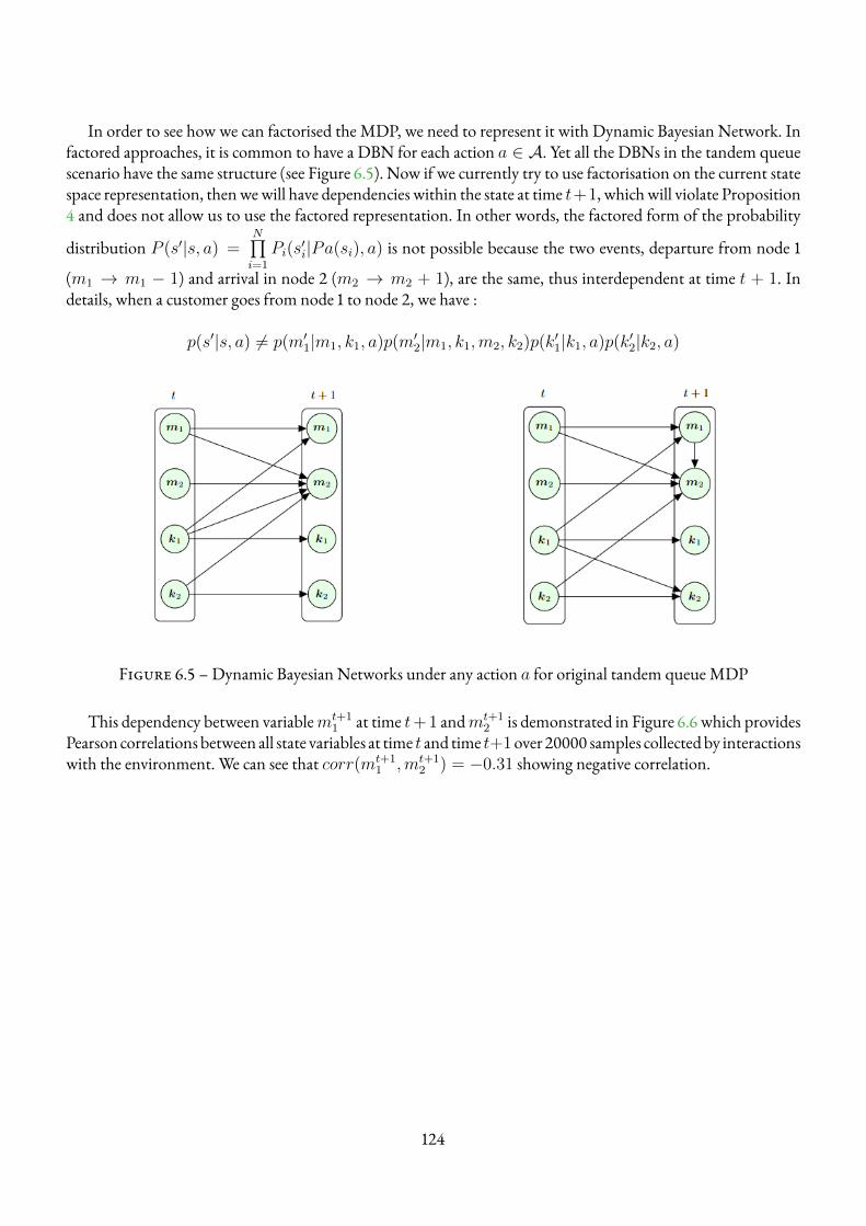
In order to see how we can factorised the MDP, we need to represent it with Dynamic Bayesian Network. Infactored approaches, it is common to have a DBN for each action a ∈ A. Yet all the DBNs in the tandem queuescenario have the same structure (see Figure 6.5). Now if we currently try to use factorisation on the current statespace representation, thenwewill have dependencies within the state at time t+1, whichwill violate Proposition4 and does not allow us to use the factored representation. In other words, the factored form of the probability

distribution P (s′|s, a) =N∏i=1

Pi(s′i|Pa(si), a) is not possible because the two events, departure from node 1

(m1 → m1 − 1) and arrival in node 2 (m2 → m2 + 1), are the same, thus interdependent at time t + 1. Indetails, when a customer goes from node 1 to node 2, we have :

p(s′|s, a) 6= p(m′1|m1, k1, a)p(m′2|m1, k1,m2, k2)p(k′1|k1, a)p(k′2|k2, a)

Figure 6.5 – Dynamic Bayesian Networks under any action a for original tandem queueMDP

This dependency between variablemt+11 at time t+ 1 andmt+1

2 is demonstrated in Figure 6.6 which providesPearson correlations between all state variables at time t and time t+1over 20000 samples collectedby interactionswith the environment. We can see that corr(mt+1

1 ,mt+12 ) = −0.31 showing negative correlation.

124

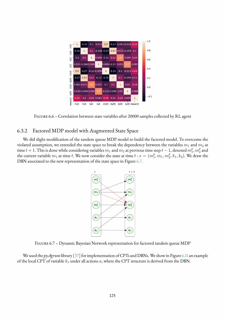
Figure 6.6 – Correlation between state variables after 20000 samples collected by RL agent

6.3.2 FactoredMDPmodel with Augmented State SpaceWe did slight modification of the tandem queue MDP model to build the factored model. To overcome the

violated assumption, we extended the state space to break the dependency between the variablesm1 andm2 attime t+ 1. This is done while considering variablesm1 andm2 at previous time step t− 1, denotedmp

1,mp2 and

the current variablem1 at time t. We now consider the state at time t : s = (mp1,m1,m

p2, k1, k2). We draw the

DBN associated to the new representation of the state space in Figure 6.7.

Figure 6.7 – Dynamic Bayesian Network representation for factored tandem queueMDP

Weused the pyAgrum library [37] for implementation of CPTs andDBNs.We show in Figure 6.11 an exampleof the local CPT of variable k1 under all actions a, where the CPT structure is derived from the DBN.

125

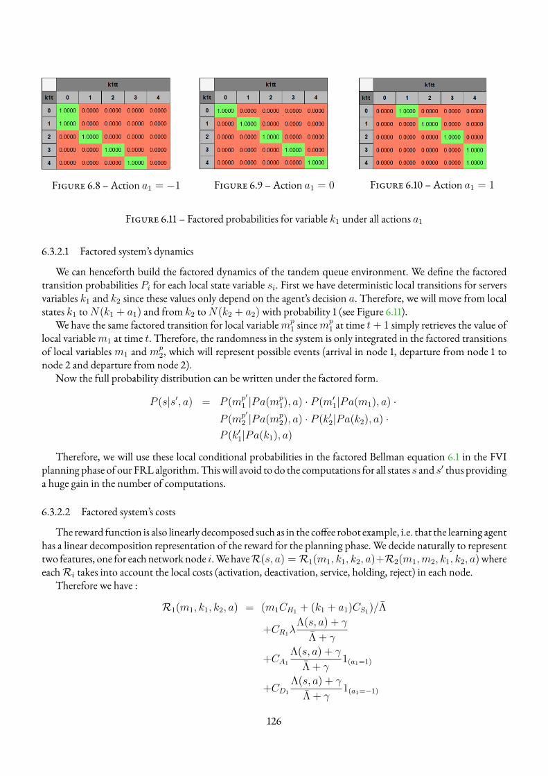
Figure 6.8 – Action a1 = −1 Figure 6.9 – Action a1 = 0 Figure 6.10 – Action a1 = 1

Figure 6.11 – Factored probabilities for variable k1 under all actions a1

6.3.2.1 Factored system’s dynamics

We can henceforth build the factored dynamics of the tandem queue environment. We define the factoredtransition probabilities Pi for each local state variable si. First we have deterministic local transitions for serversvariables k1 and k2 since these values only depend on the agent’s decision a. Therefore, we will move from localstates k1 toN(k1 + a1) and from k2 toN(k2 + a2) with probability 1 (see Figure 6.11).

We have the same factored transition for local variablemp1 sincem

p1 at time t+ 1 simply retrieves the value of

local variablem1 at time t. Therefore, the randomness in the system is only integrated in the factored transitionsof local variablesm1 andmp

2, which will represent possible events (arrival in node 1, departure from node 1 tonode 2 and departure from node 2).

Now the full probability distribution can be written under the factored form.

P (s|s′, a) = P (mp′

1 |Pa(mp1), a) · P (m′1|Pa(m1), a) ·

P (mp′

2 |Pa(mp2), a) · P (k′2|Pa(k2), a) ·

P (k′1|Pa(k1), a)

Therefore, we will use these local conditional probabilities in the factored Bellman equation 6.1 in the FVIplanning phase of our FRL algorithm.Thiswill avoid to do the computations for all states s and s′ thus providinga huge gain in the number of computations.

6.3.2.2 Factored system’s costs

The reward function is also linearly decomposed such as in the coffee robot example, i.e. that the learning agenthas a linear decomposition representation of the reward for the planning phase. We decide naturally to representtwo features, one for each network node i.We haveR(s, a) = R1(m1, k1, k2, a)+R2(m1,m2, k1, k2, a)whereeachRi takes into account the local costs (activation, deactivation, service, holding, reject) in each node.

Therefore we have :

R1(m1, k1, k2, a) = (m1CH1 + (k1 + a1)CS1)/Λ

+CR1λΛ(s, a) + γ

Λ + γ

+CA1

Λ(s, a) + γ

Λ + γ1(a1=1)

+CD1

Λ(s, a) + γ

Λ + γ1(a1=−1)

126

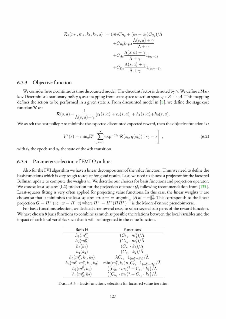
R2(m1,m2, k1, k2, a) = (m2CH2 + (k2 + a2)CS2)/Λ

+CR2k1µ1Λ(s, a) + γ

Λ + γ

+CA2

Λ(s, a) + γ

Λ + γ1(a2=1)

+CD2

Λ(s, a) + γ

Λ + γ1(a2=−1)

6.3.3 Objective functionWe consider here a continuous time discountedmodel. The discount factor is denoted by γ. We define aMar-

kov Deterministic stationary policy q as a mapping from state space to action space q : S → A. This mappingdefines the action to be performed in a given state s. From discounted model in [5], we define the stage costfunctionR as :

R(s, a)=1

Λ(s, a)+γ[c1(s, a) + c2(s, a)] + h1(s, a)+h2(s, a).

We search the best policy q to minimise the expected discounted expected reward, then the objective function is :

V ∗(s) = minqEq

[∞∑k=0

exp−γtk R(sk, q(sk)) | s0 = s

], (6.2)

with tk the epoch and sk the state of the kth transition.

6.3.4 Parameters selection of FMDP onlineAlso for the FVI algorithm we have a linear decomposition of the value function. Thus we need to define the

basis functions which is very tough to adjust for good results. Last, we need to choose a projector for the factoredBellman update to compute the weightsw. We describe our choices for basis functions and projection operator.We choose least-squares (L2)-projection for the projection operator G, following recommendation from [135].Least-squares fitting is very often applied for projecting value functions. In this case, the linear weights w arechosen so that it minimises the least-squares error w = argminw||Hw − v||22. This corresponds to the linearprojectionG = H+ (i.e.,w = H+v) whereH+ = HT (HHT )−1 is the Moore-Penrose pseudoinverse.

For basis functions selection, we decided after several tests, to select several sub-parts of the reward function.We have chosen 8 basis functions to combine as much as possible the relations between the local variables and theimpact of each local variables such that it will be integrated in the value function.

Basis H Functionsh1(mp

1) (Ch1 ·mp1)/Λ

h2(mp2) (Ch2 ·m

p2)/Λ

h3(k1) (Cs1 · k1)/Λh4(k2) (Cs2 · k2)/Λ

h5(mp1, k1, k2) λCr1 · 1(mp1=B1)/Λ

h6(mp1,m

p2, k1, k2) min(mp

1, k1)µ1Cr2 · 1(mp2=B2)/Λ

h7(mp1, k1)

((Ch1 ·m1)2 + Cs1 · k1

)/Λ

h8(mp2, k2)

((Ch1 ·m1)2 + Cs1 · k1

)/Λ

Table 6.5 – Basis functions selection for factored value iteration

127

6.4 Numerical Results

We present in this section the comparison between our method FMDP online and state-of-the-art Reinfor-cement Learning algorithms on the tandem queue system.

6.4.1 Environments and Simulation ParametersWe keep the same python Gym simulator as described in Chapter V Section 5.4. What changes now is how

the RL agent perceives the environment. In this factored approach, it has a new observation of the environmentas described above s = (mp

1,m1,mp2, k1, k2).

6.4.1.1 Cloud parameters

We first describe cloud simulations parameters.We consider two cloud scenarios of different scalesC1 : {B1 =B2 = 10, K1 = K2 = 3, µ1 = µ2 = 2, λ = 8} andC2 : {B1 = B2 = 15, K1 = K2 = 5, µ1 = µ2 = 2, λ =15}. For all these scenarios the costs parameters are the same in the two nodes : {Ca = 1, Cd = 1, Cs = 2, Ch =2, Cr = 10}.

6.4.1.2 Algorithms comparison

We compare our FMDP onlinemethod with state-of-the-art RL algorithms.We choose one model-free RLmethod : Q-Learning, one buffer-based RL method : Dyna Q and finally the conventional model-based RLmethod :MDP online. TheMDPonline algorithmworks similarly to FMDPonline.However it works directlywith the global conditional distribution P (s′|s, a). Therefore it can suffer from heavy update computations be-cause of the matrix size in large-scale systems. This is one issue our method can resolve since it only updates smallsize matrices (local conditional probabilitiesPi), and does not require excessive amount of memory for problemsin large-scale systems. We also recall that in the FVI algorithm we can use a sampling method that considers onlya subset S ′ ⊆ S of the whole state space.

6.4.1.3 Simulation and algorithms parameters

We detail here the simulation and algorithms parameters. Learning phase runs for 100 episodes of length10000 iterations. One iteration corresponds to a transition from state s with action a to state s′ with reward r.The agent runs epsilon-greedy policy over thewhole learning process, with initial epsilon set to ε = 1.Wedecreaseepsilon value after each episode with a decay rate εdec = 0.99. The discount rate is set to γ = 0.9.

6.4.2 Comparison Criteria between AlgorithmsWe compare the different algorithms during the learning phase. Performance measurements during learning

are represented by a learning curve. We look at running time of algorithms and the average reward obtained aftereach episode to compare the goodness of the RL methods. We note that RL algorithms should also be assessedoffline, e.g. with Monte-Carlo offline policy evaluation. For this purpose we need to convert the factored policyof the augmented state space for fair comparison with the classical policy. This is currently being investigated aspart of further research. Henceforth we only display the comparison during the learning process.

128

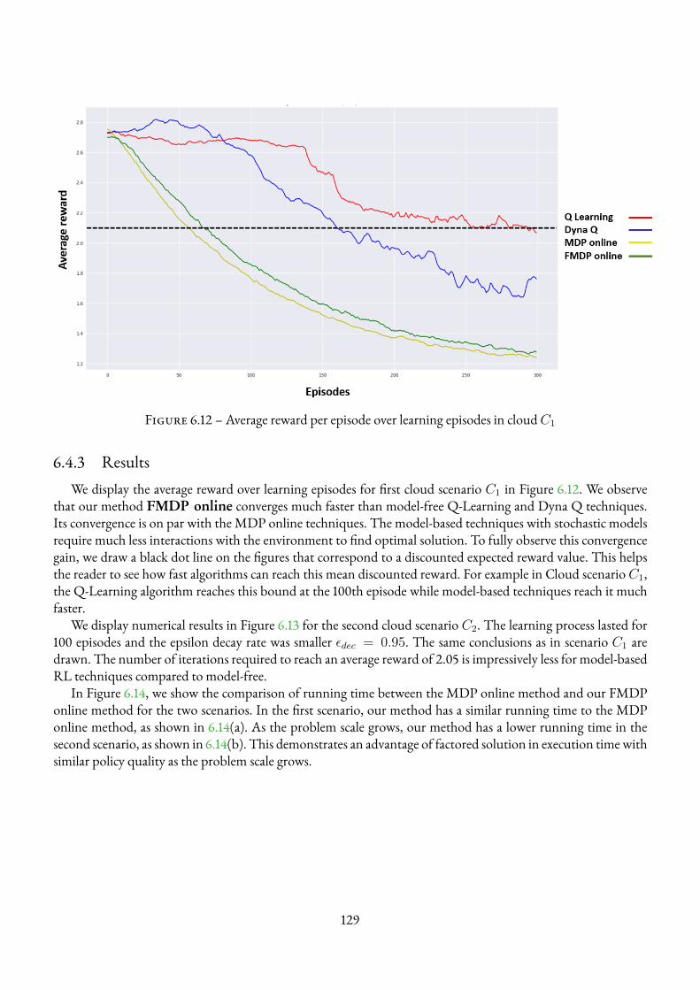
Figure 6.12 – Average reward per episode over learning episodes in cloudC1

6.4.3 ResultsWe display the average reward over learning episodes for first cloud scenario C1 in Figure 6.12. We observe

that our method FMDP online converges much faster than model-free Q-Learning and Dyna Q techniques.Its convergence is on par with the MDP online techniques. The model-based techniques with stochastic modelsrequire much less interactions with the environment to find optimal solution. To fully observe this convergencegain, we draw a black dot line on the figures that correspond to a discounted expected reward value. This helpsthe reader to see how fast algorithms can reach this mean discounted reward. For example in Cloud scenarioC1,the Q-Learning algorithm reaches this bound at the 100th episode while model-based techniques reach it muchfaster.

We display numerical results in Figure 6.13 for the second cloud scenario C2. The learning process lasted for100 episodes and the epsilon decay rate was smaller εdec = 0.95. The same conclusions as in scenario C1 aredrawn. The number of iterations required to reach an average reward of 2.05 is impressively less for model-basedRL techniques compared to model-free.

In Figure 6.14, we show the comparison of running time between the MDP online method and our FMDPonline method for the two scenarios. In the first scenario, our method has a similar running time to the MDPonline method, as shown in 6.14(a). As the problem scale grows, our method has a lower running time in thesecond scenario, as shown in 6.14(b). This demonstrates an advantage of factored solution in execution timewithsimilar policy quality as the problem scale grows.

129

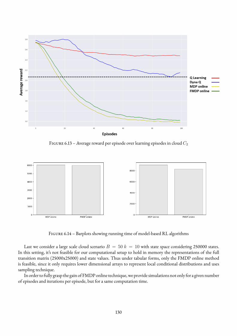
Figure 6.13 – Average reward per episode over learning episodes in cloudC2

Figure 6.14 – Barplots showing running time of model-based RL algorithms

Last we consider a large scale cloud scenario B = 50 k = 10 with state space considering 250000 states.In this setting, it’s not feasible for our computational setup to hold in memory the representations of the fulltransition matrix (25000x25000) and state values. Thus under tabular forms, only the FMDP online methodis feasible, since it only requires lower dimensional arrays to represent local conditional distributions and usessampling technique.

Inorder to fully grasp the gainofFMDPonline technique,weprovide simulationsnot only for a givennumberof episodes and iterations per episode, but for a same computation time.

130

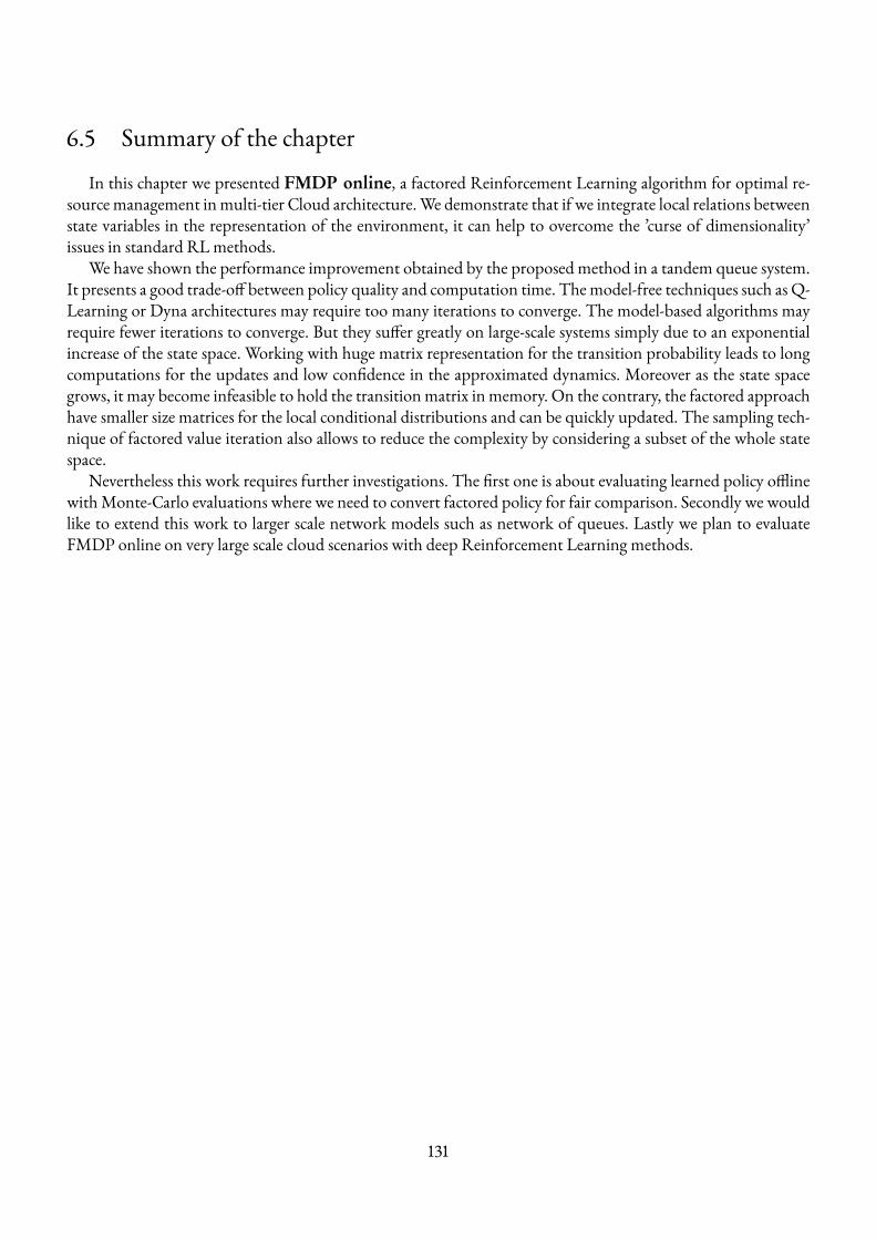
6.5 Summary of the chapter

In this chapter we presented FMDP online, a factored Reinforcement Learning algorithm for optimal re-source management inmulti-tier Cloud architecture.We demonstrate that if we integrate local relations betweenstate variables in the representation of the environment, it can help to overcome the ’curse of dimensionality’issues in standard RLmethods.

We have shown the performance improvement obtained by the proposed method in a tandem queue system.It presents a good trade-off between policy quality and computation time. Themodel-free techniques such as Q-Learning or Dyna architectures may require too many iterations to converge. The model-based algorithms mayrequire fewer iterations to converge. But they suffer greatly on large-scale systems simply due to an exponentialincrease of the state space. Working with huge matrix representation for the transition probability leads to longcomputations for the updates and low confidence in the approximated dynamics. Moreover as the state spacegrows, it may become infeasible to hold the transitionmatrix in memory. On the contrary, the factored approachhave smaller size matrices for the local conditional distributions and can be quickly updated. The sampling tech-nique of factored value iteration also allows to reduce the complexity by considering a subset of the whole statespace.

Nevertheless this work requires further investigations. The first one is about evaluating learned policy offlinewithMonte-Carlo evaluations where we need to convert factored policy for fair comparison. Secondly we wouldlike to extend this work to larger scale network models such as network of queues. Lastly we plan to evaluateFMDP online on very large scale cloud scenarios with deep Reinforcement Learning methods.

131

CHAPTER 7

CAUSAL REINFORCEMENT LEARNING FORMULTI-TIERNETWORK

Up to now, we have seen different model-based approaches to learn auto-scaling policies in Cloud environ-ments such as a one physical node system or a more complex scenario with multi-tier architectures. The majorissues encountered is about the curse of dimensionality that occurs when we consider larger scale Cloud envi-ronments. First model-free RL methods highly suffer to converge. Secondly, the use of tabular model-based RLalgorithms (see Chapter V) can improve performance regarding speed of convergence and policy quality but stillhave trouble to handle very large scale scenarios, precisely when addressing learning objects implementation butalso convergence. Instead of investigating the approximation path for improvement with neural networks as arepresentative tool of environment models, we decided to focus on the structural properties of the environmentsto be integrated in the learning agent’s knowledge. We considered the factored framework developed in ChapterVI which has obtained good performance regarding the improvement for implementation and considering hi-gher scale scenarios. Yet the factored representation is still a tabular approach and also has difficulty in addressingvery large problems. We believe that a causal approach can provide even better enhancements by going furtherin the understanding of environment variables relations. This causal dimension goes beyond the associational re-presentation proposed in the factored framework. The benefits can be numerous. Among those are the increasedcapability of copying with high-scale systems, the explainability of the obtained policies, improved convergencespeed, as well as capability of dealing with hidden variables or unobserved confounders. Our focus in this chapterwill be the two last aspects. In this regard, this chapter acts as an orthogonal view : we are more concerned withMDP environments with particular structure (hidden variables, unobserved confounders, etc.) than very largesystems.

Therefore in this chapter we propose to unify causal reasoning in reinforcement learning algorithms to acce-lerate convergence with counterfactuals and deal with Cloud environments with unobserved state variables thatcan have confounding effects or not.We first providemore detailed background about theCausality domain thenpropose a generalised formalism forMDPenvironment representationwithStructural CausalModels (SCM) thatare defined in the causality background section. After this combination of causality and reinforcement learningformalism, we evaluate Causal Reinforcement Learning (CRL) algorithms on the multi-tier Cloud environment,considering several scenarios : the initial tandem queue, the partially observable tandem queue withMMPP arri-vals and the tandem queue with unobserved confounders.

The chapter contributions are listed in the following :∗ Generalisation of Structural Causal Model formalism for any MDP environment and Counterfactual rea-soning;

132

∗ Proposal of a counterfactual model-free RL algorithm;∗ Assessment of causal RL methods in tandem queue environments.

7.1 Introduction to causality : Pearl’s Causal HierarchyIn order to fully understand the integration of causal reasoning in the reinforcement learning scheme, we first

provide elements of causality. Cause-and-effect relationships play a key role in how we perceive and make senseof the world around us, how we interact with it and, ultimately, how we comprehend ourselves. Almost twodecades ago, computer scientist Judea Pearl [3] made a breakthrough in understanding causality by proposingand studying the “Ladder of Causation”, a framework that showcases the distinct roles of seeing, doing, andimagining. We summarise in this section his vision and its proposal for a mathematical formalism of causality,namely structural causal models. For this purpose, we follow the description given by Bareinboim et al. in [20].A SCM naturally defines a hierarchy of concepts, described as the “ladder of causation” which Bareinboim et al.have been calling the Pearl Causal Hierarchy, or PCH. There exist three layers :Associational, Interventional andCounterfactual (see Figure 7.1).

Figure 7.1 – Pearl’s causal hierarchy representation of the world (Figure from [20]

Definition 12 (Structural Causal Model [20]). We define a structural causal model SCMMC as a 4-tuple <V,U,F , P (U) >where :— U = {U1, U2, . . . , Uk} is a set of exogenous (unobserved) variables, determined by factors outside the

model ;— V = {V1, V2, . . . , Vn} are called endogenous (observed) and are determinedby other variables in themodel

– that is, variables in U ∪ V ;— F = {f1, f2, . . . , fn} is a set of causal assignments such that fi maps variables from Ui ∪ Pai to Vi.∀i = 1, . . . , n, vi ← fi(Pai, ui), i.e. the value of vi will change caused by its parents Pai and noise ui ;

— P (U) is the distribution of noises variables.It is assumed that the causal assignments fi are invariant, except if intervention forces them to change.

7.1.1 Layer 1 - ObservationalIf you let the system behaves by itself and just observe it evolving, then you can observe the joint distribution

of endogenous variables P (V ) which is defined by :

133

Definition 13 (Observational distribution [20]). An SCMMC =< U, V,F , P (U) > defines a joint probabi-lity distribution PMC(V ) such that for each Y ⊆ V : PMC(y) =

∑u|Y (u)=y

P (u) where Y (u) is the expression

for Y after evaluation withF and U = u.In this setting, we only rely on observational data with no interventions in the system.

7.1.2 Layer 2 - InterventionalSecondly, one agent (human, software) can interact with an environment by intervening in the system. The

data collected in this setting will be interventional.Definition 14 (Interventional SCM [20]). LetM be a causal model,X a set of variables in V , and x a particularrealisation ofX . A submodelMx ofM is the causal modelMx =< U, V,Fx, P (U) >, where Fx = {fi :Vi /∈ X} ∪ {X ← x}. In other words, an interventional SCM has a subset of endogenous variables where theircausal assignments has been changed by intervention.

Notice that this intervention is a do-operatorwhich in Pearl’s terminology is amathematical operator, denoteddo(X = x)which simulates physical interventions by deleting certain functions from themodel, replacing themwith a constantX = x, while keeping the rest of the model unchanged. Naturally, this interventional world issimilar to reinforcement learning/MDP scenarios where an autonomous agent interacts with the environmentby intervening in the system, therefore changing directly values of some endogenous variables or forcing causalassignments to change. However, PCH goes further and define a third layer : the counterfactual world that givesthe ability to learning agents for imagining.

7.1.3 Layer 3 - Counterfactual : the imaginary worldThe counterfactual mode is an imaginary world where an agent can measure the possible effect of non-taken

interventions, that is, thinking about alternative ways the world could be. In other worlds, it can evaluate theoutcomes of imaginary decisions that would have happened in a given situation (or evidence).Definition 15 (Evidence). We define E an evidence of a systemM the realisations of the environment variablesat a given time t. The evidence E is therefore the expression of the endogenous and exogenous variables E ={u1, . . . , uk, v1, . . . , vn}. It does not depend on whether there was an intervention or not in the system; it onlydepicts the systems values at a given time.

In the RL paradigm, when the learning agent interacts with the environment, it observes the state of the sys-tem s and decides to act according to its policy q(s). Rollouts (or trajectories) resulting from this state-action paircan be propagated backwards for updating value functions or policies (as we have seen thorough this documentwith model-free or model-based RL techniques). However, this backpropagation update is done based on thefact that there was a specific evidence E at time twhen agent did action a in state s. One possibility to update thevalue function for this pair (s, a) is to visit it infinitely many times (which is an objective in RL for convergence).However, counterfactual reasoning can do this update in the meantime by evaluating the outcome (new stateand reward) of other actions not-taken and under the same evidence that occurred. This reasoning brings a sup-plementary knowledge and more powerful learning process since the agent can evaluate the outcomes of manydecisions in a given state s and under the same evidence. The counterfactual reasoning is possible if the agent isprovided the SCM of the world and is based on three principles that we describe below :— Abduction : Discover noise realisations u after deciding action a in the environment va. In other words,

the agent discovers the evidence E of the system and more generally updates conditional probability distri-butions p(u|va) ;

134

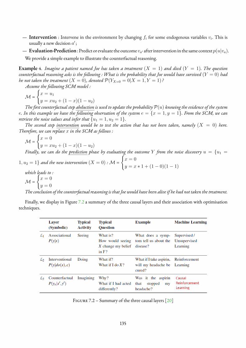
— Intervention : Intervene in the environment by changing fi for some endogenous variables vi. This isusually a new decision a′ ;

— Evaluation-Prediction : Predict or evaluate theoutcomeva′ after intervention in the same contextp(u|va).We provide a simple example to illustrate the counterfactual reasoning.

Example 4. Imagine a patient named Joe has taken a treatment (X = 1) and died (Y = 1). The questioncounterfactual reasoning asks is the following : What is the probability that Joe would have survived (Y = 0) hadhe not taken the treatment (X = 0), denoted P(YX=0 = 0|X = 1, Y = 1) ?

Assume the following SCM model :

M =

{x = u1

y = xu2 + (1− x)(1− u2)

The first counterfactual step abduction is used to update the probabilityP(u) knowing the evidence of the systeme. In this example we have the following observation of the system e = {x = 1, y = 1}. From the SCM, we canretrieve the noise values and infer that {u1 = 1, u2 = 1}.

The second step intervention would be to test the action that has not been taken, namely (X = 0) here.Therefore, we can replace x in the SCM as follows :

M =

{x = 0

y = xu2 + (1− x)(1− u2)

Finally, we can do the prediction phase by evaluating the outcome Y from the noise discovery u = {u1 =

1, u2 = 1} and the new intervention (X = 0) :M =

{x = 0

y = x ∗ 1 + (1− 0)(1− 1)

which leads to :

M =

{x = 0

y = 0

The conclusion of the counterfactual reasoning is that Joe would have been alive if he had not taken the treatment.

Finally, we display in Figure 7.2 a summary of the three causal layers and their association with optimisationtechniques.

Figure 7.2 – Summary of the three causal layers [20]

135

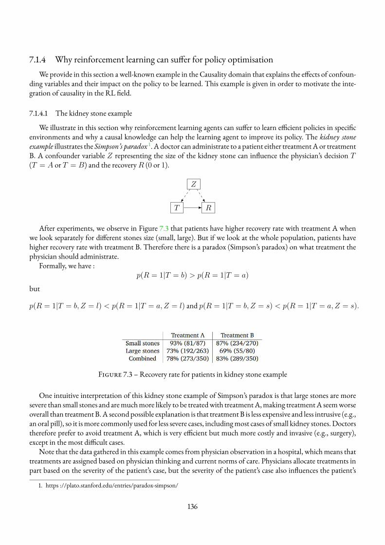
7.1.4 Why reinforcement learning can suffer for policy optimisationWe provide in this section a well-known example in the Causality domain that explains the effects of confoun-

ding variables and their impact on the policy to be learned. This example is given in order to motivate the inte-gration of causality in the RL field.

7.1.4.1 The kidney stone example

We illustrate in this section why reinforcement learning agents can suffer to learn efficient policies in specificenvironments and why a causal knowledge can help the learning agent to improve its policy. The kidney stoneexample illustrates the Simpson’s paradox 1. A doctor can administrate to a patient either treatmentAor treatmentB. A confounder variable Z representing the size of the kidney stone can influence the physician’s decision T(T = A or T = B) and the recoveryR (0 or 1).

T R

Z

After experiments, we observe in Figure 7.3 that patients have higher recovery rate with treatment A whenwe look separately for different stones size (small, large). But if we look at the whole population, patients havehigher recovery rate with treatment B. Therefore there is a paradox (Simpson’s paradox) on what treatment thephysician should administrate.

Formally, we have :p(R = 1|T = b) > p(R = 1|T = a)

but

p(R = 1|T = b, Z = l) < p(R = 1|T = a, Z = l) and p(R = 1|T = b, Z = s) < p(R = 1|T = a, Z = s).

Figure 7.3 – Recovery rate for patients in kidney stone example

One intuitive interpretation of this kidney stone example of Simpson’s paradox is that large stones are moresevere than small stones and aremuchmore likely to be treatedwith treatmentA,making treatmentA seemworseoverall than treatment B.A second possible explanation is that treatment B is less expensive and less intrusive (e.g.,an oral pill), so it ismore commonly used for less severe cases, includingmost cases of small kidney stones.Doctorstherefore prefer to avoid treatment A, which is very efficient but much more costly and invasive (e.g., surgery),except in the most difficult cases.

Note that the data gathered in this example comes from physician observation in a hospital, whichmeans thattreatments are assigned based on physician thinking and current norms of care. Physicians allocate treatments inpart based on the severity of the patient’s case, but the severity of the patient’s case also influences the patient’s

1. https ://plato.stanford.edu/entries/paradox-simpson/

136

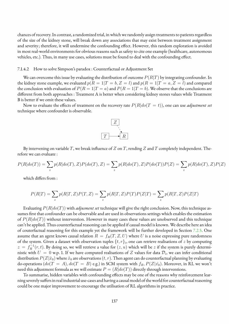
chances of recovery. In contrast, a randomized trial, inwhichwe randomly assign treatments to patients regardlessof the size of the kidney stone, will break down any associations that may exist between treatment assignmentand severity ; therefore, it will undermine the confounding effect. However, this random exploration is avoidedin most real-world environments for obvious reasons such as safety to cite one example (healthcare, autonomousvehicles, etc.). Thus, in many use cases, solutions must be found to deal with the confounding effect.

7.1.4.2 How to solve Simpson’s paradox : Counterfactual or Adjustment Set

We can overcome this issue by evaluating the distribution of outcomeP (R|T ) by integrating confounder. Inthe kidney stone example, we evaluated p(R = 1|T = b, Z = l) and p(R = 1|T = a, Z = l) and comparedthe conclusion with evaluation of P (R = 1|T = a) and P (R = 1|T = b). We observe that the conclusions aredifferent from both approaches : Treatment A is better when considering kidney stones values while TreatmentB is better if we omit these values.

Now to evaluate the effects of treatment on the recovery rate P (R|do(T = t)), one can use adjustment settechnique where confounder is observable.

T R

Z

By intervening on variable T , we break influence ofZ on T , rendingZ and T completely independent. The-refore we can evaluate :

P (R|do(T )) =∑z

p(R|do(T ), Z)P (do(T ), Z) =∑z

p(R|do(T ), Z)P (do(T ))P (Z) =∑z

p(R|do(T ), Z)P (Z)

which differs from :

P (R|T ) =∑z

p(R|T, Z)P (T, Z) =∑z

p(R|T, Z)P (T )P (Z|T ) =∑z

p(R|T, Z)P (Z|T )

Evaluating P (R|do(T ))with adjusment set technique will give the right conclusion. Now, this technique as-sumes first that confounder can be observable and are used in observations settings which enables the estimationof P (R|do(T )) without intervention. However in many cases these values are unobserved and this techniquecan’t be applied. Thus counterfactual reasoning can be applied if causal model is known.We describe here an ideaof couterfactual reasoning for this example yet the framework will be further developed in Section 7.2.5. Oneassume that an agent knows causal relation R = fR(T, Z, U) where U is a noise expressing pure randomnessof the system. Given a dataset with observation tuples {t, r}i, one can retrieve realisations of z by computingz = f−1

R (r, t). By doing so, we will retrieve a value for (z, u) which will be z if the system is purely determi-nistic with U = 0 w.p. 1. If we have computed realisations of Z values for data Di, we can infer conditionaldistributionP (Z|x0)where x0 are observations (t, r). Then agent can do counterfactual planning by evaluatingdo-operations (do(T = A), do(T = B) e.g.) in SCM system with fR, P (Z|x0). Moreover, in RL we won’tneed this adjustment formula as we will estimate P = (R|do(T )) directly through interventions.

To summarise, hidden variables with confounding effects may be one of the reasons why reinforcement lear-ning severely suffers in real industrial use-cases andhaving a causalmodel of theworld for counterfactual reasoningcould be one major improvement to encourage the utilisation of RL algorithms in practice.

137

7.2 Causal Reinforcement Learning : Formalism and EnvironmentsThis section ought to build a general formalism for Reinforcement Learning methods with causal model ap-

proaches. We first give an overview of the recent literature works about Causal Reinforcement Learning. Then,we display the main difference for representing Markov Decision Process environment with usual models andwith causal models. Afterwards, we describe possible existing MDP environments, next provide definitions forSCM equivalent description of the MDP environment models. Finally, we provide the counterfactual reasoningprocess in different MDP environments.

7.2.1 Causal Reinforcement Learning literatureVery recently, researchers [30, 47, 153] ought to merge the causal and reinforcement learning fields. To in-

troduce this new emerging field, we first provide understanding about causal and initial MDP representations.Secondly, we give a well-known example in the causality field that can explain why RL can fail in some environ-ments. Next, we give an overview of very recent works that studied this integration by providing CRL techniquesand formalism. We have seen that reinforcement learning domain was associated with interventional layer 2 ofthe causality domain. As for the kidney stone example where counterfactual reasoning can bring benefit for theoptimal policy search, the idea of CausalReinforcement Learning is to bring this counterfactual reasoning in rein-forcement learning methods. This emerging domain has received very few attention in the past years but startsto grow. The works [153] and [30] are two works dealing with causal reinforcement learning and counterfactualreasoning. They both demonstrates that counterfactual reasoning can bring policy optimisation improvement inspecific scenarios, compared to SoTA reinforcement learning methods. Bareinboim et al. [153] focus onMarkovdecision processes with unobserved confounders (MDPUC ) environment, where a set of endogenous variablesH is hidden to theRL agent and these variables confound the agent’s policy q(S,H) and the rewardR. However,in their formalism they integrate unobserved confounders (UC) inside exogenous set of variables, regarding theSCMdefinition 12.On the other hand, theDeepmind team [30] restricts its scope on partially observableMarkovdecision process (POMDP) environment where they integrate a noise hiding some state features to the agent inthe SOKOBAN environment 2.

Both papers represents the MDP environment with structural causal model (SCM), described in section 7.1.Definition 16 ([153]). AMarkovDecision Process with Unobserved Confounders (MDPUCs) is an augmentedSCMMwith finite action domainA, state domain S , and reward variableR :— γ ∈ [0, 1) is the discount factor ;— U(t) is the exogenous variable at round t ;— V (t) = A(t)∪R(t)∪S(t) is the set of endogenous (observable) variables at round t withA(t) the action

space, S(t) the state space andR(t) the reward function;— F = {fa; fy; fs} is the set of structural equations relative to V such that A(t) = fa(s(t);u(t)) =

q(s(t);u(t)), R(t) = fr(a(t); s(t);u(t)) and S(t) = fs(a(t− 1); s(t− 1);u(t− 1)) ;— P(u) encodes the probability distribution over the exogenous variables U.The work [30] also consider an SCM modelling of the MDP environment but does not formally define

this translation MDP → SCM . Yet they propose in their paper a solution to equivalently describe state-transitional modelsM with causal assignments. For generalisation of dynamics modelling in causal model andstate-transitional model, one can represent both structure equivalently. In [30] is stated a lemma for this equiva-lent representation.

2. https ://fr.wikipedia.org/wiki/Sokoban

138

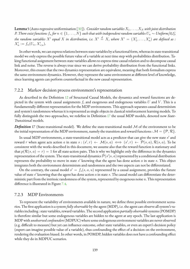
Lemma 5 (Auto-regressive uniformisation [30]). Consider random variablesX1, . . . , XN with joint distributionP. There exist functions fn for n ∈ {1, . . . , N} such that with independent random variablesUn ∼Uniform[0,1],the random variables X ′ equal X in distribution, i.e. X ′ d

= X , where X ′ = (X ′1, . . . , X′n) are defined as :

X ′n := fn(Un, X′<n).

Inotherwords,we can express relationsbetween state variables by a functional form,whereas in state-transitionalmodel we only express the possible future value of a variable at next time step with probabilities distribution. Ta-king functional assignment between state variables allows to express time causal relation and to decompose causallink and noise. The reverse is always true since we can derive probability distribution from the functional links.Moreover, this ensure that the two dynamics representation are equivalent, meaning that both formalism expressthe same environment dynamics. However, they represent the same environment at different level of knowledge,since learning agents can perform counterfactual in the new causal representation.

7.2.2 Markov decision process environment’s representationAs described in the Definition 12 of Structural Causal Models, the dynamics and reward functions are de-

picted in the system with causal assignments fi and exogenous and endogenous variables U and V . This is afundamentally different representation for theMDP environments. This approach separates causal determinismand system’s randomness whereas it is represented as single objects in classical reinforcement learning models. Tofully distinguish the two approaches, we redefine in Definition 17 the usual MDP models, denoted now State-Transitional models.Definition 17 (State-transitional model). We define the state-transitional modelM of the environment to bethe initial representation of theMDP environment, namely the transition and reward functions :M = {P ,R}.

In usual MDP environments, a state-transitional model acts as a predictor that can give the new state s′ andreward r when agent acts action a in state s : (s′, r) ← M(s, a) ⇐⇒ (s′, r) ← P(s, a),R(s, a). To beconsistent with the works described in this document, we assume also that the reward function is stationary andthat p(R(s, a) = r) = 1 for all state-action pairs. This is why we highlight only the difference in the dynamicsrepresentationof the system.The state-transitional dynamicsP(s′|s, a) representedby a conditional distributionrepresents the probability to move in state s′ knowing that the agent has done action a in state s. This objectintegrates both the environment determinism and randomness and the two aspects can not be differentiated.

On the contrary, the causal model s′ = fs(s, a, u) represented by a causal assignment, provides the futurevalue of state s′ knowing that the agent has done action a in state s. The causal model can differentiate the deter-ministic part from the intrinsic randomness of the system, represented by exogenous noiseu. This representationdifference is illustrated in Figure 7.4.

7.2.3 MDP EnvironmentsTo represent the variability of environments available in nature, we define three possible environment scena-

rios. The first application is a system fully observable by the agent (MDP), i.e. the agent can observe all system’s va-riables including : state variables, reward variables. The second application partially observable systems (POMDP)is therefore similar but some endogenous variables are hidden to the agent at any epoch. The last application isMDPwithunobserved confounders (MDPUC)where some endogenous environment variables are never observed(e.g. difficult to measure) but yet can influence outcome, other state variables, or even an expert’s decision policy(expert can imagine possible value of a variable), thus confounding the effect of a decision on the environment,rendering the evaluation biased. In other words, in POMDP, hidden variables does not have a confounding effectwhile they do inMDPUC scenarios.

139

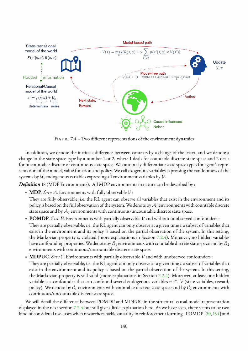
Figure 7.4 – Two different representations of the environment dynamics

In addition, we denote the intrinsic difference between contexts by a change of the letter, and we denote achange in the state space type by a number 1 or 2, where 1 deals for countable discrete state space and 2 dealsfor uncountable discrete or continuous state space. We cautiously differentiate state space types for agent’s repre-sentation of the model, value function and policy. We call exogenous variables expressing the randomness of thesystems by U , endogenous variables expressing all environment variables by V .Definition 18 (MDP Environments). All MDP environments in nature can be described by :∗ MDP. EnvA. Environments with fully observable V :They are fully observable, i.e. the RL agent can observe all variables that exist in the environment and itspolicy is based on the full observation of the system.Wedenote byA1 environmentswith countable discretestate space and byA2 environments with continuous/uncountable discrete state space.∗ POMDP. Env B. Environments with partially observable V and without unobserved confounders :They are partially observable, i.e. the RL agent can only observe at a given time t a subset of variables thatexist in the environment and its policy is based on the partial observation of the system. In this setting,the Markovian property is violated (more explanations in Section 7.2.4). Moreover, no hidden variableshave confounding properties.We denote byB1 environments with countable discrete state space and byB2

environments with continuous/uncountable discrete state space.∗ MDPUC. Env C. Environments with partially observable V and with unobserved confounders :They are partially observable, i.e. the RL agent can only observe at a given time t a subset of variables thatexist in the environment and its policy is based on the partial observation of the system. In this setting,the Markovian property is still valid (more explanations in Section 7.2.4). Moreover, at least one hiddenvariable is a confounder that can confound several endogenous variables v ∈ V (state variables, reward,policy). We denote by C1 environments with countable discrete state space and by C2 environments withcontinuous/uncountable discrete state space.

We will detail the difference between POMDP and MDPUC in the structural causal model representationdisplayed in the next section 7.2.4 but still give a little explanation here. As we have seen, there seems to be twokind of considered use-cases when researchers tackle causality in reinforcement learning : POMDP [30, 154] and

140

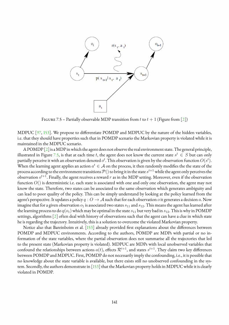
Figure 7.5 – Partially observable MDP transition from t to t+ 1 (Figure from [2])

MDPUC [97, 153]. We propose to differentiate POMDP and MDPUC by the nature of the hidden variables,i.e. that they should have properties such that in POMDP scenario theMarkovian property is violated while it ismaintained in the MDPUC scenario.

APOMDP[2] is aMDP inwhich the agent does not observe the real environment state.The general principle,illustrated in Figure 7.5, is that at each time t, the agent does not know the current state st ∈ S but can onlypartially perceive it with an observation denoted ot. This observation is given by the observation functionO(st).When the learning agent applies an action at ∈ A on the process, it then randomly modifies the the state of theprocess according to the environment transitionsP() to bring it in the state st+1 while the agent only perceives theobservation ot+1. Finally, the agent receives a reward r as in the MDP setting. Moreover, even if the observationfunction O() is deterministic i.e. each state is associated with one and only one observation, the agent may notknow the state. Therefore, two states can be associated to the same observation which generates ambiguity andcan lead to poor quality of the policy. This can be simply understand by looking at the policy learned from theagent’s perspective. It updates a policy q : O → A such that for each observation o it generates a decision a. Nowimagine that for a given observation o1 is associated two states s11 and s12. This means the agent has learned afterthe learning process to do q(o1)whichmay be optimal in the state s11 but very bad in s12. This is why in POMDPsettings, algorithms [2] often deal with history of observations such that the agent can have a clue in which statehe is regarding the trajectory. Intuitively, this is a solution to overcome the violatedMarkovian property.

Notice also that Bareinboim et al. [153] already provided first explanations about the differences betweenPOMDP and MDPUC environments. According to the authors, POMDP are MDPs with partial or no in-formation of the state variables, where the partial observation does not summarise all the trajectories that ledto the present state (Markovian property is violated). MDPUC are MDPs with local unobserved variables thatconfound the relationships between actions a(t), effectsRt+1, and states st+1. They claim two key differencesbetween POMDP andMDPUC. First, POMDPdo not necessarily imply the confounding, i.e., it is possible thatno knowledge about the state variable is available, but there exists still no unobserved confounding in the sys-tem. Secondly, the authors demonstrate in [153] that theMarkovian property holds inMDPUCwhile it is clearlyviolated in POMDP.

141

7.2.4 SCM representation of MDP environmentsWebuild a bridge between the three families ofMDP environments :MDP, POMDPandMDPUCby forma-

lising a general SCMfor anyMDPenvironmentmodels. Formally, we differentiate unobserved confounders fromnoise exogenous variables and consider them as endogenous variables that can be unobserved by the agent. Thuswe consider a physical system or environment E by having two distinct parts. The first one is the deterministiccausal relation partwith causal assignmentsF between environment endogenous state variablesS = (s1, ..., sn),reward variableRwhich is a function of state variables si and action variablesA = (a1, ..., al). The second classrepresents natural inherent randomness of the system with exogenous noise variables U = (u1, ...uk) that candisturb deterministic relations.Definition 19 (Markov Decision Process with SCM). AMarkov Decision Process can be represented by a struc-tural causal modelMwith finite action domainA, state domain S , and reward variableR :— γ ∈ [0, 1) is the discount factor ;— U t is the set of exogenous variables at time t determined by factors outside the model and representing the

randomness of the system. All noise variables u are independent from each other ;— V t = At ∪ Rt ∪ St is the set of endogenous (potentially observable) variables at time t. This includes all

environment variables potentially observable by the agent ;— F = {fa; fr; fs} is the set of structural equations relative toV such that at = fa(s

t;uta) ∼ q(at|st), Rt =fr(a

t; st;ut) ∼ P (Rt|st, at) and St+1 = fs(at; st;ut) ∼ P (st+1|st, at). Note that policy q is determi-

nistic if uta = 0 else stochastic ;— P(U) encodes the probability distribution over the exogenous variables U.Definition 19 defines the structural causal model representation of aMDPwhere the state s is represented as a

single object.We have seen in Chapter VI that the state could be represented by a vector of state variables si in thefactored approach. For this purpose, we also propose a definition for structural causal model representation offactoredMDP. And finally, this latest formalism is themost suitable since wewill also deal with causal graphs andlocal causal relations in the SCM approach. Therefore, the following definition 20 will be themain formalism forMDP representation by SCM.Definition 20 (Causal Markov Decision Process). A FactoredMarkov Decision Process can be represented by astructural causal modelM with finite action domainA, state domain S = {s1, . . . , sN}, and reward variableR :— γ ∈ [0, 1) is the discount factor ;— U t = {ut1, . . . , utk, uta, utr} is the set of exogenous variables at time t determined by factors outside the

model and representing the randomness of the system. All noise variables u are independent from eachother ;

— V t = At ∪ Rt ∪ St is the set of endogenous (potentially observable) variables at time t. This includes allenvironment variables potentially observable by the agent. If some variables in V are hidden at some timest, we are in POMDP orMDPUC;

— F = {fa; fr; fs1 , . . . , fsN} is the set of structural equations relative to V such that at = fa(st;uta) ∼

q(st),Rt+1 = fr(at, Pa(Rt);utr) ∼ P (Rt+1|Pa(Rt), at) and

∀i = {1, . . . , N}, st+1i = fsi(a

t;Pa(sti);uti) ∼ Pi(s

t+1i |Pa(sti), a

t)

, where Pa(.) ∈ S denotes the parents variables values at previous time step;— P(U) encodes the probability distribution over the exogenous variables U.

142

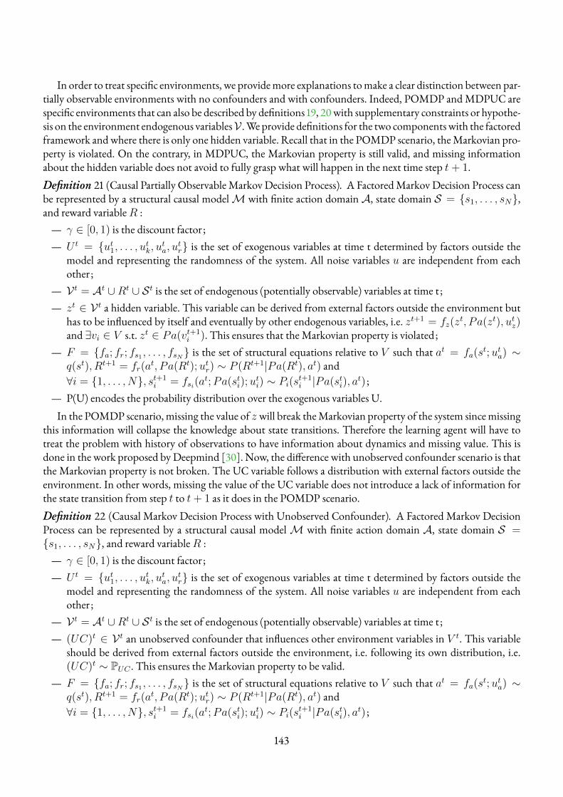
In order to treat specific environments, we providemore explanations tomake a clear distinction between par-tially observable environments with no confounders and with confounders. Indeed, POMDP andMDPUC arespecific environments that can also be described by definitions 19, 20with supplementary constraints or hypothe-sis on the environment endogenous variablesV .We provide definitions for the two componentswith the factoredframework and where there is only one hidden variable. Recall that in the POMDP scenario, theMarkovian pro-perty is violated. On the contrary, in MDPUC, the Markovian property is still valid, and missing informationabout the hidden variable does not avoid to fully grasp what will happen in the next time step t+ 1.Definition 21 (Causal Partially ObservableMarkov Decision Process). A FactoredMarkov Decision Process canbe represented by a structural causal modelM with finite action domainA, state domain S = {s1, . . . , sN},and reward variableR :— γ ∈ [0, 1) is the discount factor ;— U t = {ut1, . . . , utk, uta, utr} is the set of exogenous variables at time t determined by factors outside the

model and representing the randomness of the system. All noise variables u are independent from eachother ;

— V t = At ∪Rt ∪ St is the set of endogenous (potentially observable) variables at time t ;— zt ∈ V t a hidden variable. This variable can be derived from external factors outside the environment but

has to be influenced by itself and eventually by other endogenous variables, i.e. zt+1 = fz(zt, Pa(zt), utz)

and ∃vi ∈ V s.t. zt ∈ Pa(vt+1i ). This ensures that the Markovian property is violated ;

— F = {fa; fr; fs1 , . . . , fsN} is the set of structural equations relative to V such that at = fa(st;uta) ∼

q(st), Rt+1 = fr(at, Pa(Rt);utr) ∼ P (Rt+1|Pa(Rt), at) and

∀i = {1, . . . , N}, st+1i = fsi(a

t;Pa(sti);uti) ∼ Pi(s

t+1i |Pa(sti), a

t) ;— P(U) encodes the probability distribution over the exogenous variables U.In the POMDP scenario, missing the value of z will break theMarkovian property of the system sincemissing

this information will collapse the knowledge about state transitions. Therefore the learning agent will have totreat the problem with history of observations to have information about dynamics and missing value. This isdone in the work proposed byDeepmind [30]. Now, the difference with unobserved confounder scenario is thatthe Markovian property is not broken. The UC variable follows a distribution with external factors outside theenvironment. In other words, missing the value of the UC variable does not introduce a lack of information forthe state transition from step t to t+ 1 as it does in the POMDP scenario.Definition 22 (Causal Markov Decision Process with Unobserved Confounder). A Factored Markov DecisionProcess can be represented by a structural causal modelM with finite action domain A, state domain S ={s1, . . . , sN}, and reward variableR :— γ ∈ [0, 1) is the discount factor ;— U t = {ut1, . . . , utk, uta, utr} is the set of exogenous variables at time t determined by factors outside the

model and representing the randomness of the system. All noise variables u are independent from eachother ;

— V t = At ∪Rt ∪ St is the set of endogenous (potentially observable) variables at time t ;— (UC)t ∈ V t an unobserved confounder that influences other environment variables in V t. This variable

should be derived from external factors outside the environment, i.e. following its own distribution, i.e.(UC)t ∼ PUC . This ensures the Markovian property to be valid.

— F = {fa; fr; fs1 , . . . , fsN} is the set of structural equations relative to V such that at = fa(st;uta) ∼

q(st), Rt+1 = fr(at, Pa(Rt);utr) ∼ P (Rt+1|Pa(Rt), at) and

∀i = {1, . . . , N}, st+1i = fsi(a

t;Pa(sti);uti) ∼ Pi(s

t+1i |Pa(sti), a

t) ;

143

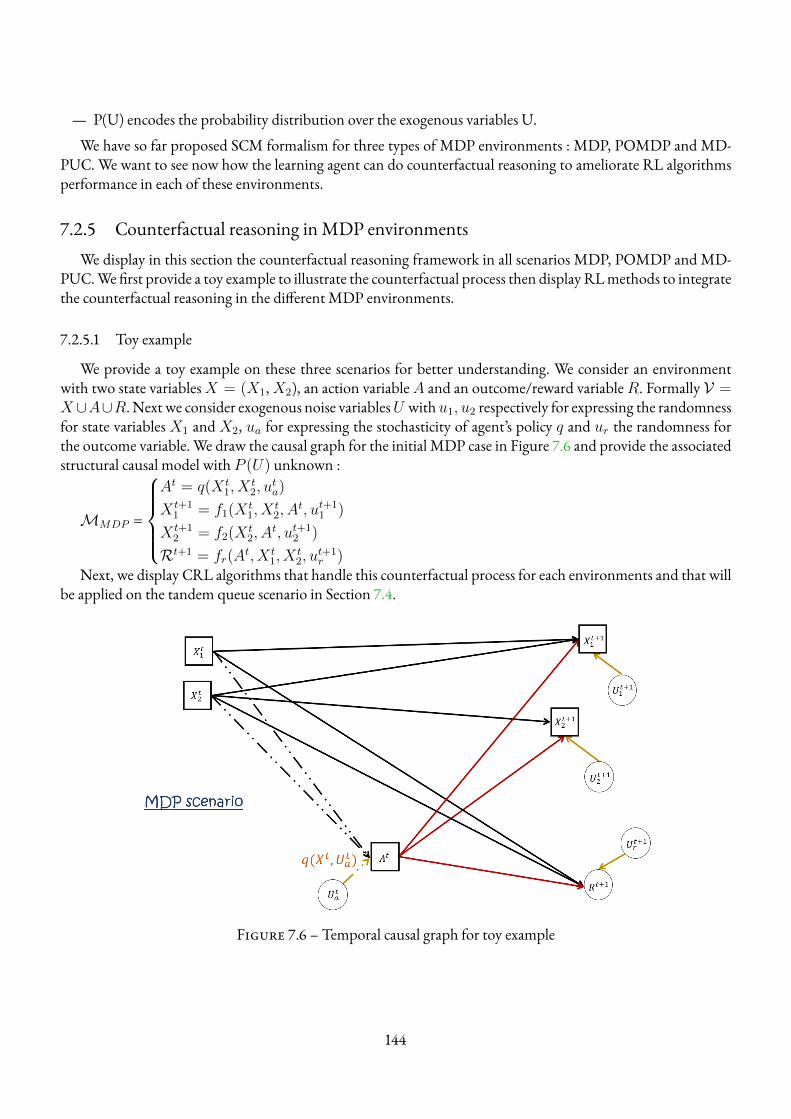
— P(U) encodes the probability distribution over the exogenous variables U.We have so far proposed SCM formalism for three types of MDP environments : MDP, POMDP and MD-

PUC. We want to see now how the learning agent can do counterfactual reasoning to ameliorate RL algorithmsperformance in each of these environments.

7.2.5 Counterfactual reasoning inMDP environmentsWe display in this section the counterfactual reasoning framework in all scenarios MDP, POMDP and MD-

PUC.We first provide a toy example to illustrate the counterfactual process then display RLmethods to integratethe counterfactual reasoning in the different MDP environments.

7.2.5.1 Toy example

We provide a toy example on these three scenarios for better understanding. We consider an environmentwith two state variablesX = (X1,X2), an action variableA and an outcome/reward variableR. Formally V =X∪A∪R. Next we consider exogenous noise variablesU withu1, u2 respectively for expressing the randomnessfor state variables X1 and X2, ua for expressing the stochasticity of agent’s policy q and ur the randomness forthe outcome variable. We draw the causal graph for the initial MDP case in Figure 7.6 and provide the associatedstructural causal model with P (U) unknown :

MMDP =

At = q(X t

1, Xt2, u

ta)

X t+11 = f1(X t

1, Xt2, A

t, ut+11 )

X t+12 = f2(X t

2, At, ut+1

2 )

Rt+1 = fr(At, X t

1, Xt2, u

t+1r )

Next, we display CRL algorithms that handle this counterfactual process for each environments and that willbe applied on the tandem queue scenario in Section 7.4.

Figure 7.6 – Temporal causal graph for toy example

144

7.2.5.2 MDP counterfactual

In the MDP scenario, since all endogenous variables are observed, the counterfactual reasoning can be utili-sed to infer information about exogenous noise variables U , i.e. about the system’s randomness similarly as thelearning of stochastic transitions in the state-transitional model. This is the first step of counterfactual reasoning,corresponding to the abduction phase and we will show the process for one single variable si.

Abduction In general, the causal assignment associated to a variable si takes as input parent’s variables at timet of the local variable si, the agent’s decision at and a noise uti, then outputs the value of si at time t+ 1.

st+1i = fi(Pa(st+1

i ), at, ut+1i )

For a given tuple (Pa(st+1i ), at, st+1

i ), obtained from data, the agent can infer the noise value ut+1i by taking

the inverse of the causal assignment fi under some assumptions on the function form :

ut+1i = f−1

i (st+1i , Pa(st+1

i ), at)

We denote by ui the discovered noise value. Therefore the agent has now the evidence of the system at time twhen he did action at and can infer the outcome of non taken decisions a′ ∈ A \ {a}, by doing the interventionand the prediction phases with its updated SCM. Concretely in our example, its new SCMwould be :

MMDP =

At = q(X t

1, Xt2, ua)

X t+11 = f1(X t

1, Xt2, A

t, u1)

X t+12 = f2(X t

2, At, u2)

Rt+1 = fr(At, X t

1, Xt2, ur)

Intervention With its updated SCM, the learning agent can imagine a new intervention (the counterfactualdecision) in the systemby doing action a′ in the system do(At = a′). In our example, this would change the SCMas follows :

MMDP =

a′ ← do(At = a′)

X t+11 = f1(X t

1, Xt2, a′, u1)

X t+12 = f2(X t

2, a′, u2)

Rt+1 = fr(a′, X t

1, Xt2, ur)

Prediction Finally, it can predict or evaluate the outcome of the system by using causal assignments and theevidence to predict what would action a′ do :

st+1i = fi(Pa(st+1

i ), a′, ui)

In our example, this would mean to evaluateX t+11 ,X t+1

2 and rt+1 from the SCM computations.Notice that we have shown the counterfactual process on one data sample by discovering the value of noises

and using these evidence values to predict new outcomes. This can be generalised by considering distribution ofnoises, i.e. the agent has an a priori distribution for noise variablesPprior(U)which can be updated from the noisevalues discovery with Bayesian learning techniques, leading toPposterior(U). Finally, the evaluation of non takendecisions is made by simulating the system with the updated SCM that includes the a posteriori distributions ofnoise variables. This allows for a broader and more generic evaluation of counterfactuals since it considers largerpossibilities for the noise values.

145

Finally, we depict in Algorithm 30 a causal Dyna-Q-Learning method with the counterfactual reasoning todiscover noise values and do planning by evaluating counterfactuals. This method can be seen as a data augmen-tation technique since the agent will be able to plan and update itsQ-function for all possible actions at each timestep. At each time step, when the agent performs action a in state s, it recovers from the SCM and the abduc-tion phase the noise values of the system (We denote in the pseudocode this process by InferenceSCM ). Next itupdates the Q-function for all the non taken actions with the SCM.

Algorithm 30: Counterfactual-based data augmentation RL (CDYNA - Causal Dyna-Q-Learning)Input:Q0, q0, α learning rate, γ discount rate, εOutput: q∗, Q∗

Data: SCMM is known,P(U) is unknown/* Loop until end of episodes or criterion */

1 for e ∈MaxEpisode do2 Select state s ∈ S , s = (s1, . . . , sn) // Initial state3 for i ∈MaxIteration do4 Take action a ∈ Awith ε-greedy policy // Action selection5 Observe s′ and reward r(s, a) and collect tuple< s, a, r, s′ > // Collecting tuples data6 Q(s, a)← Q(s, a) + α [r(s, a) + γmax′aQ(s′, a′)−Q(s, a)] // Update Q

7 Ui ← InferenceSCM(s,a,r,s’) // Abduction/* Counterfactual evaluation of non-chosen actions */

8 for a′ ∈ A \ a do9 Replace action a′ in the SCM // Intervention

10 Calculate r′, s′′ = F (s, a′, Ui) // Prediction11 Q(s, a′)← Q(s, a′) + α [r′ + γmaxa′′Q(s′′, a′′)−Q(s, a)] // Update Q

7.2.5.3 POMDP counterfactual

Let us now consider the partially observable scenario with no confounding variable, i.e. it exists some endoge-nous variables in V that are unobserved and the Markovian property is violated. In this context, we should treatthe problem by using history of data to gain information about transitions between two time steps. Suppose thatin our example the endogenous variableX2 is unobserved. This leads to the following SCM that the agent carrieswhere the agent’s policy is only influenced by variableX1 :

MPOMDP =

At = q(X t

1, uta)

X t+11 = f1(X t

1, Xt2, A

t, ut+11 )(

X t+12 = f2(X t

2, At, ut+1

2 ))unobserved

Rt+1 = fr(At, X t

1, Xt2, U

t+1r )

We display the partially observable example in Figure 7.7.

146

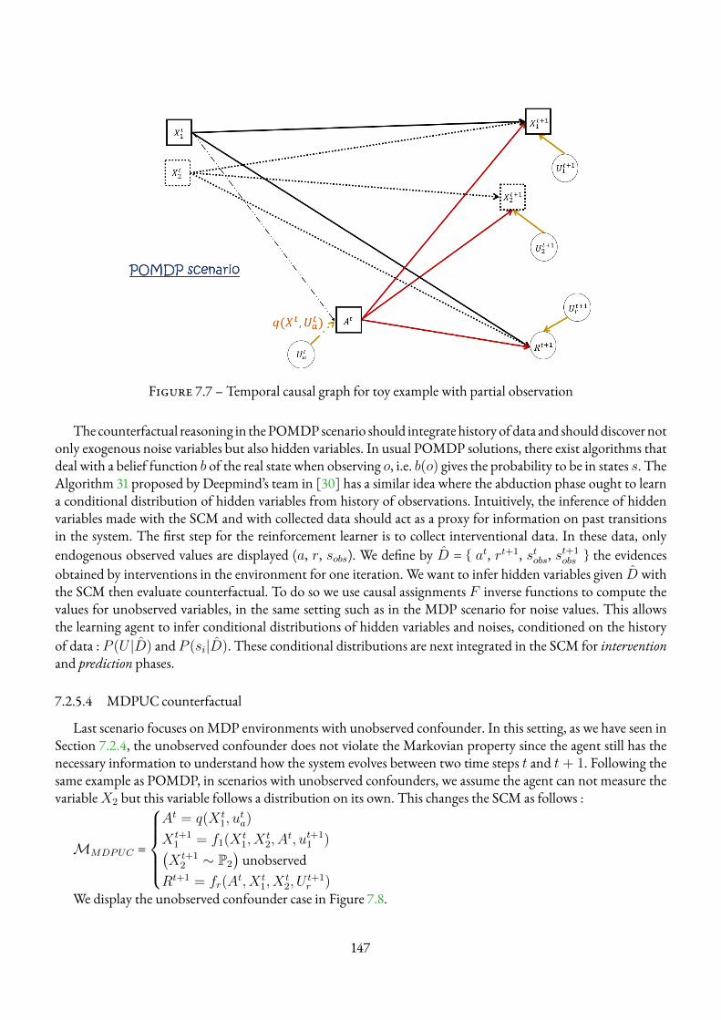
Figure 7.7 – Temporal causal graph for toy example with partial observation

The counterfactual reasoning in thePOMDPscenario should integrate history of data and shoulddiscover notonly exogenous noise variables but also hidden variables. In usual POMDP solutions, there exist algorithms thatdeal with a belief function b of the real state when observing o, i.e. b(o) gives the probability to be in states s. TheAlgorithm 31 proposed by Deepmind’s team in [30] has a similar idea where the abduction phase ought to learna conditional distribution of hidden variables from history of observations. Intuitively, the inference of hiddenvariables made with the SCM and with collected data should act as a proxy for information on past transitionsin the system. The first step for the reinforcement learner is to collect interventional data. In these data, onlyendogenous observed values are displayed (a, r, sobs). We define by D = { at, rt+1, stobs, s

t+1obs } the evidences

obtained by interventions in the environment for one iteration. We want to infer hidden variables given D withthe SCM then evaluate counterfactual. To do so we use causal assignments F inverse functions to compute thevalues for unobserved variables, in the same setting such as in the MDP scenario for noise values. This allowsthe learning agent to infer conditional distributions of hidden variables and noises, conditioned on the historyof data : P (U |D) and P (si|D). These conditional distributions are next integrated in the SCM for interventionand prediction phases.

7.2.5.4 MDPUC counterfactual

Last scenario focuses onMDP environments with unobserved confounder. In this setting, as we have seen inSection 7.2.4, the unobserved confounder does not violate the Markovian property since the agent still has thenecessary information to understand how the system evolves between two time steps t and t + 1. Following thesame example as POMDP, in scenarios with unobserved confounders, we assume the agent can not measure thevariableX2 but this variable follows a distribution on its own. This changes the SCM as follows :

MMDPUC =

At = q(X t

1, uta)

X t+11 = f1(X t

1, Xt2, A

t, ut+11 )(

X t+12 ∼ P2

)unobserved

Rt+1 = fr(At, X t

1, Xt2, U

t+1r )

We display the unobserved confounder case in Figure 7.8.

147

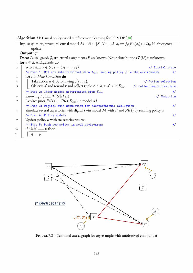
Algorithm 31: Causal policy-based reinforcement learning for POMDP [30]Input: q0 = µ0, structural causal modelM : ∀i ∈ |S|,∀a ∈ A, si := fi(Pa(si)) + Ui, N : frequency

updateOutput: q∗

Data: Causal graph G, structural assignments F are known, Noise distributionsP(U) is unknown1 for e ∈MaxEpisode do2 Select state s ∈ S , s = (s1, . . . , sk) // Initial state

/* Step 1: Collect interventional data Dobs running policy q in the environment */3 for i ∈MaxIteration do4 Take action a ∈ A following q(s, uA). // Action selection5 Observe s′ and reward r and collect tuple< s, a, r, s′ > inDobs // Collecting tuples data

/* Step 2: Infer noises distribution from Dobs */6 Knowing F , inferP(U|Dobs) // Abduction7 Replace priorP(U)← P(U|Dobs) in modelM

/* Step 3: Digital twin simulation for counterfactual evaluation */8 Simulate several trajectories with digital twin modelMwith F andP(U) by running policy µ

/* Step 4: Policy update */9 Update policy µwith trajectories returns

/* Step 5: Push new policy in real environment */10 if e%N == 0 then11 q ← µ

Figure 7.8 – Temporal causal graph for toy example with unobserved confounder

148

In the MDPUC context, there is no need to treat the problem with historical data since the Markovian pro-perty is not violated. Therefore, the counterfactual reasoning process here would only infer an a posteriori dis-tribution of the hidden variableX2, not conditioned on history of data. Again, this learned distribution wouldserve as an element of the new SCM to generate rollouts for counterfactual planning. The algorithm that we willuse in the experimental results Section 7.4 in the Algorithm 30 but the InferenceSCM() part will also discover thevalue of the UC variable.

7.2.5.5 Overview of counterfactual in MDP environments

To summarise the counterfactual reasoning in Reinforcement Learning, the learning agent is provided theSCMof theworld (relations between environment variables, causal assignments) and can infer information abouthidden and noise variables from collected interventional data and by taking the inverse of causal functions. De-pending on the scenario (POMDP or MPDUC), the agent will deal with historical data or not. Finally, it willevaluate counterfactual decisions based on its updated SCM with distributions or discovered values for the hid-den variables. Notice that this counterfactual planning is different than initial planning of model-based RL tech-niques. The simulated trajectories are generated by differentiating the causal deterministic part and the random-ness part of the system with noises distributions. This creates more precise trajectories illustrated with the follo-wing example.

Example 5. Planning in Model-based RL : The agent will generate rollouts with its model P and R such thats′, r ← P(s′, s, a),R(s, a) and will update its policy or value function according to this sample (or trajectory).Yet, the evidence of the environment that occurred when the agent visited (s, a) in the past are lost in the state-transitional model because there is no distinction between causal assignments and randomness.

Planning in Counterfactual RL : The agent will generate rollouts with its SCMmodel and inferred distributionsof hidden and noise variables such that s′, r ← F (s, a, u), P (U),R(s, a, u). This sampling process is more precisebecause it considers the evidence information that occurred when the agent has visited the state-action pair (s, a)in the past.

In a nutshell, the counterfactual process should provide a gain in usual MDP systems by accelerating theconvergence because the counterfactual process could evaluate multiple non-taken decisions more quickly. Ho-wever the main benefit will reside in context with hidden variables where non causal models will suffer to inferinformation about unobserved variables and can be potentially biased resulting in learned policies with poorquality. This is what we will demonstrate in Section 7.4 with an application for the tandem queue Cloud envi-ronment.

7.3 Causal modelling of multi-tier Cloud architecturesThis section presents the application of CRL techniques inmulti-tier Cloud architectures. It consists of refor-

malising the MDP model with SCMmodelling and comparing counterfactual reinforcement learning methodswith SoTARL algorithms in different environments (MDP, POMDP,MPDUC). However, we let the treatmentof POMDP cases in perspective and only deal with the initial tandem queue environment and scenario withunobserved confounders, namely MDP andMDPUC environments.

149

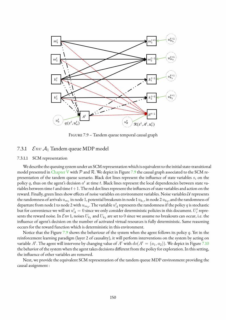
Figure 7.9 – Tandem queue temporal causal graph

7.3.1 EnvA1 Tandem queueMDPmodel

7.3.1.1 SCM representation

Wedescribe thequeuing systemunder anSCMrepresentationwhich is equivalent to the initial state-transitionalmodel presented in Chapter V withP andR. We depict in Figure 7.9 the causal graph associated to the SCM re-presentation of the tandem queue scenario. Black dot lines represent the influence of state variables si on thepolicy q, thus on the agent’s decision at at time t. Black lines represent the local dependencies between state va-riables between time t and time t+1. The red dot lines represent the influences of state variables and action on thereward. Finally, green lines show effects of noise variables on environment variables. Noise variables U representsthe randomness of arrivalsum1 in node 1, potential breakouts in node 1uk1 , in node 2uk2 , and the randomness ofdeparture from node 1 to node 2with um2 . The variable utA represents the randomness if the policy q is stochasticbut for convenience we will set utA = 0 since we only consider deterministic policies in this document.U t

r repre-sents the reward noise. In Env 1, noises Uk1 and Uk2 are set to 0 since we assume no breakouts can occur, i.e. theinfluence of agent’s decision on the number of activated virtual resources is fully deterministic. Same reasoningoccurs for the reward function which is deterministic in this environment.

Notice that the Figure 7.9 shows the behaviour of the system when the agent follows its policy q. Yet in thereinforcement learning paradigm (layer 2 of causality), it will perform interventions on the system by acting onvariableAt. The agent will intervene by changing value ofAt with do(At = (a1, a2)). We depict in Figure 7.10the behavior of the systemwhen the agent takes decisions different from the policy for exploration. In this setting,the influence of other variables are removed.

Next, we provide the equivalent SCM representation of the tandem queueMDP environment providing thecausal assignment :

150

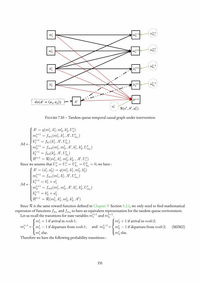
Figure 7.10 – Tandem queue temporal causal graph under intervention

M =

At = q(mt1, k

t1,m

t2, k

t2, U

ta)

mt+11 = fm1(mt

1, kt1, A

t, U tm1

)

kt+11 = fk1(kt1, A

t, U tk1

)

mt+12 = fm2(mt

1,mt2, A

t, kt1, kt2, U

tm2

)

kt+12 = fk2(kt2, A

t, U tk2

)

Rt+1 = R(mt1, k

t1,m

t2, k

t2, , A

t, U tr)

Since we assume that U ta = U t

r = U tk1

= U tk2

= 0, we have :

M =

At = (at1, at2) = q(mt

1, kt1,m

t2, k

t2)

mt+11 = fm1(mt

1, kt1, A

t, U tm1

)

kt+11 = kt1 + at1mt+1

2 = fm2(mt1,m

t2, A

t, kt1, kt2, U

tm2

)

kt+12 = kt2 + at2Rt+1 = R(mt

1, kt1,m

t2, k

t2, A

t)

SinceR is the same reward function defined in Chapter V Section 5.2.1, we only need to find mathematicalexpression of functions fm1 and fm2 to have an equivalent representation for the tandem queue environment.

Let us recall the transitions for state variablesmt+11 andmt+1

2 .

mt+11 =

mt

1 + 1 if arrival in node1;

mt1 − 1 if departure from node1;

mt1 else.

and mt+12 =

mt

2 + 1 if arrival in node2;

mt2 − 1 if departure from node2; (M1M2)

mt2 else.

Therefore we have the following probability transitions :

151

P (mt+11 |Pa(m1), at) =

λ

Λif arrival inN1;

µ1(kt1 + at1)

Λif departure fromN1;

Λ− λ− µ1(kt1 + at1)

Λelse.

and

P (mt+12 |Pa(m2), at) =

µ1(kt1 + at1)

Λif arrival inN2;

µ2(kt2 + at2)

Λif departure fromN2;

Λ− µ1(kt1 + at1)− µ2(kt2 + at2)

Λelse.

We propose to rewrite the following dynamics in the SCM form, i.e. with causal assignments to express whatwill be the next value of state variables at time t+ 1. (M1M2) can be rewritten by :mt+1

1 = mt1 + 1(event=arrival) − 1(event=departure)

⇔ mt+11 = mt

1 + 1Um1≤λ/Λ− 1Um1≤(λ+µ1(kt1+at1))/Λ where U t

m1∼ Unif [0, 1]

andmt+1

2 = mt2 + 1Utm2

≤λ/Λ − 1Utm2≤(λ+µ1(kt1+at1))/Λ where U t

m2∼ Unif [0, 1]

Finally, we have the SCM representing tandem queue dynamics with :

M=

At = q(mt1, k

t1,m

t2, k

t2)

mt+11 = mt

1 + 1Ut+1m1≤λ/Λ − 1Um1≤(λ+µ1(kt1+at1))/Λ where U t+1

m1∼ Unif [0, 1]

kt+11 = kt1 + at1mt+1

2 = mt2 + 1Ut+1

m1≤(λ+µ1(kt1+at1))/Λ − 1Ut+1

m2≤(µ1(kt1+at1))+µ2(kt2+at2))/Λ where U t+1

m2∼ Unif [0, 1]

kt+12 = kt2 + at2Rt+1 = R(mt

1, kt1,m

t2, k

t2, A

t)

Notice that we could also have found the functions with the inverse-CDFmethod and the proposed methodfrom the Deepmind’s work [30] in Lemma 5.

7.3.1.2 Counterfactual calculations

Recall that we consider theMDP scenario first where the agent can observe the full environment state. Accor-ding to Section 7.2.5, it only requires to discover the exogenous noise values with the counterfactual reasoning.Thus, for one experience tuple, the agent can discover the noises realisations with inverse causal assignments inthe following way :

U =

{U t+1m1

= f−1m1(mt

1, kt1, A

t,mt+11 )

U t+1m2

= f−1m2(mt

1,mt2, A

t, kt2,mt+12 )

Concretely, from a data sample (s, a, r, s′) it computes from the SCM the noise values um1 and um2 :

U =

{um1 = f−1

m1(m1, k1 + a1,m′1)

um2 = f−1m2(m1,m2, k1 + a1, k2 + a2,m

′2)

Once the agent has the noise realisations under a specific experience tuple, it can evaluate counterfactual deci-sions followingAlgorithm30.As inChapterV andChapterVI the learning agent observes from the environmentsamples (s, a, r, s′) and ought to learn the dynamics of the system by discovering exogenous noise variables. We

152

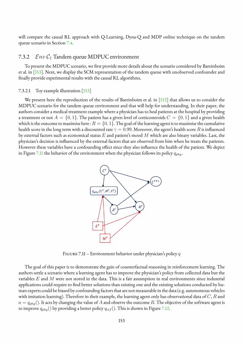
will compare the causal RL approach with Q-Learning, Dyna-Q and MDP online technique on the tandemqueue scenario in Section 7.4.

7.3.2 Env C1 Tandem queueMDPUC environmentTo present the MDPUC scenario, we first provide more details about the scenario considered by Bareinboim

et al. in [153]. Next, we display the SCM representation of the tandem queue with unobserved confounder andfinally provide experimental results with the causal RL algorithms.

7.3.2.1 Toy example illustration [153]

We present here the reproduction of the results of Bareinboim et al. in [153] that allows us to consider theMDPUC scenario for the tandem queue environment and that will help for understanding. In their paper, theauthors consider a medical treatment example where a physician has to heal patients at the hospital by providinga treatment or not A = {0, 1}. The patient has a given level of corticosteroids C = {0, 1} and a given healthwhich is the outcome tomaximise here :R = {0, 1}. The goal of the learning agent is tomaximise the cumulativehealth score in the long term with a discounted rate γ = 0.99. Moreover, the agent’s health scoreR is influencedby external factors such as economical status E and patient’s moodM which are also binary variables. Last, thephysician’s decision is influenced by the external factors that are observed from him when he treats the patients.However these variables have a confounding effect since they also influence the health of the patient. We depictin Figure 7.11 the behavior of the environment when the physician follows its policy qphy.

Figure 7.11 – Environment behavior under physician’s policy q

The goal of this paper is to demonstrate the gain of counterfactual reasoning in reinforcement learning. Theauthors settle a scenario where a learning agent has to improve the physician’s policy from collected data but thevariables E andM were not stored in the data. This is a fair assumption in real environments since industrialapplications could require to find better solutions than existing one and the existing solutions conducted by hu-man experts could be biased by confounding factors that are notmeasurable in the data (e.g. autonomous vehicleswith imitation learning). Therefore in their example, the learning agent only has observational data ofC ,R anda = qphy(). It acts by changing the value ofA and observe the outcomeR. The objective of the software agent isto improve qphy() by providing a better policy qctf (). This is shown in Figure 7.12.

153

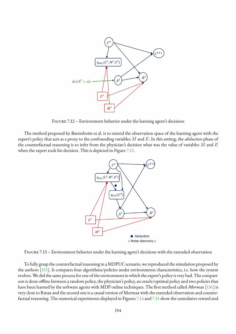
Figure 7.12 – Environment behavior under the learning agent’s decisions

The method proposed by Bareinboim et al. is to extend the observation space of the learning agent with theexpert’s policy that acts as a proxy to the confounding variablesM andE. In this setting, the abduction phase ofthe counterfactual reasoning is to infer from the physician’s decision what was the value of variablesM and Ewhen the expert took his decision. This is depicted in Figure 7.13.

Figure 7.13 – Environment behavior under the learning agent’s decisions with the extended observation

To fully grasp the counterfactual reasoning in aMDPUC scenario, we reproduced the simulation proposed bythe authors [153]. It compares four algorithms/policies under environments characteristics, i.e. how the systemevolves.We did the same process for one of the environment inwhich the expert’s policy is very bad. The compari-son is done offline between a random policy, the physician’s policy, an oracle/optimal policy and two policies thathave been learned by the software agents withMDP online techniques. The first method calledMormax [136] isvery close to Rmax and the second one is a causal version ofMormax with the extended observation and counter-factual reasoning. The numerical experiments displayed in Figures 7.14 and 7.15 show the cumulative reward and

154

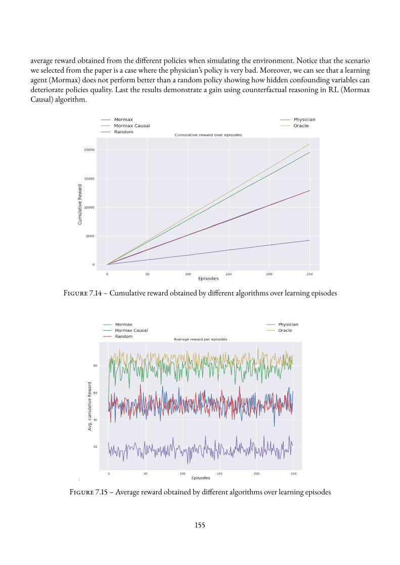
average reward obtained from the different policies when simulating the environment. Notice that the scenariowe selected from the paper is a case where the physician’s policy is very bad. Moreover, we can see that a learningagent (Mormax) does not perform better than a random policy showing how hidden confounding variables candeteriorate policies quality. Last the results demonstrate a gain using counterfactual reasoning in RL (MormaxCausal) algorithm.

Figure 7.14 – Cumulative reward obtained by different algorithms over learning episodes

Figure 7.15 – Average reward obtained by different algorithms over learning episodes

155

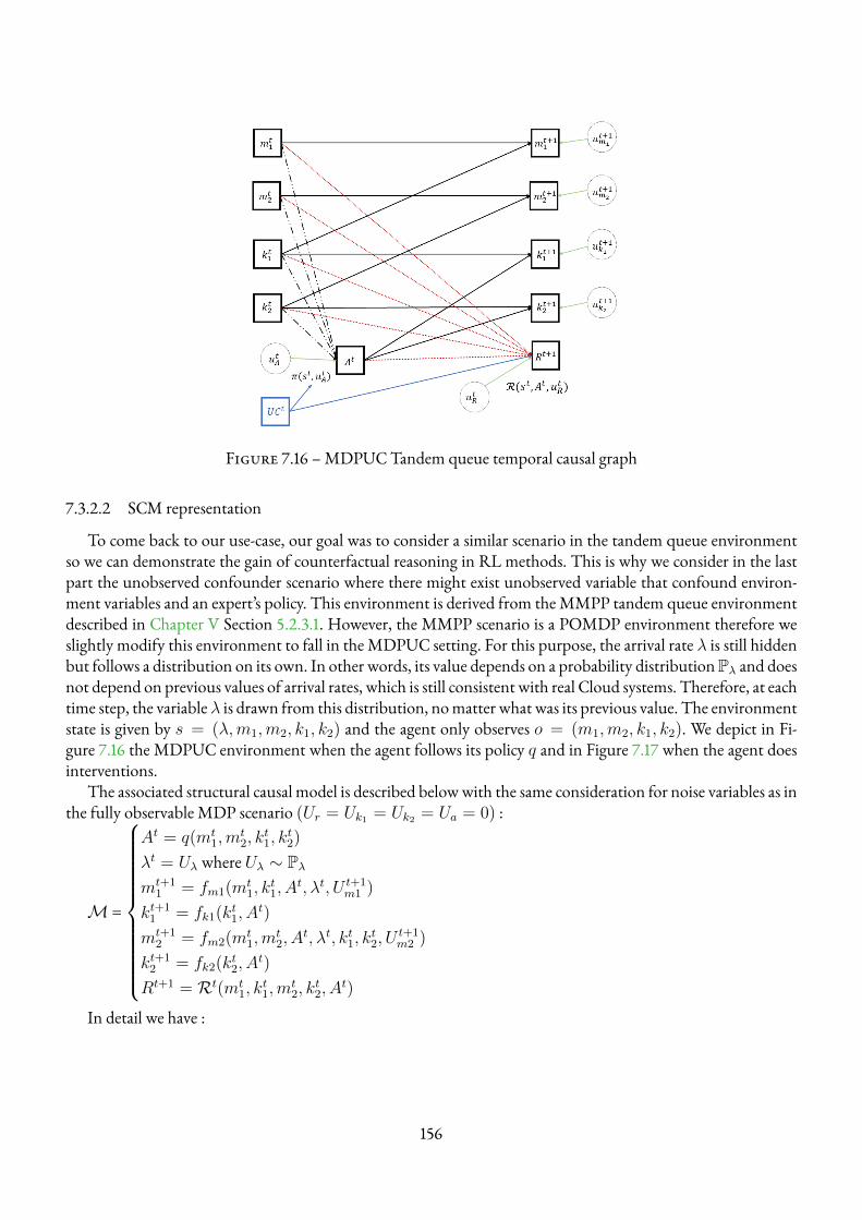
Figure 7.16 –MDPUCTandem queue temporal causal graph

7.3.2.2 SCM representation

To come back to our use-case, our goal was to consider a similar scenario in the tandem queue environmentso we can demonstrate the gain of counterfactual reasoning in RL methods. This is why we consider in the lastpart the unobserved confounder scenario where there might exist unobserved variable that confound environ-ment variables and an expert’s policy. This environment is derived from theMMPP tandem queue environmentdescribed in Chapter V Section 5.2.3.1. However, the MMPP scenario is a POMDP environment therefore weslightly modify this environment to fall in theMDPUC setting. For this purpose, the arrival rate λ is still hiddenbut follows a distribution on its own. In other words, its value depends on a probability distributionPλ and doesnot depend on previous values of arrival rates, which is still consistent with real Cloud systems. Therefore, at eachtime step, the variableλ is drawn from this distribution, nomatter what was its previous value. The environmentstate is given by s = (λ,m1,m2, k1, k2) and the agent only observes o = (m1,m2, k1, k2). We depict in Fi-gure 7.16 the MDPUC environment when the agent follows its policy q and in Figure 7.17 when the agent doesinterventions.

The associated structural causal model is described belowwith the same consideration for noise variables as inthe fully observable MDP scenario (Ur = Uk1 = Uk2 = Ua = 0) :

M =

At = q(mt1,m

t2, k

t1, k

t2)

λt = Uλ where Uλ ∼ Pλmt+1

1 = fm1(mt1, k

t1, A

t, λt, U t+1m1 )

kt+11 = fk1(kt1, A

t)

mt+12 = fm2(mt

1,mt2, A

t, λt, kt1, kt2, U

t+1m2 )

kt+12 = fk2(kt2, A

t)

Rt+1 = Rt(mt1, k

t1,m

t2, k

t2, A

t)

In detail we have :

156

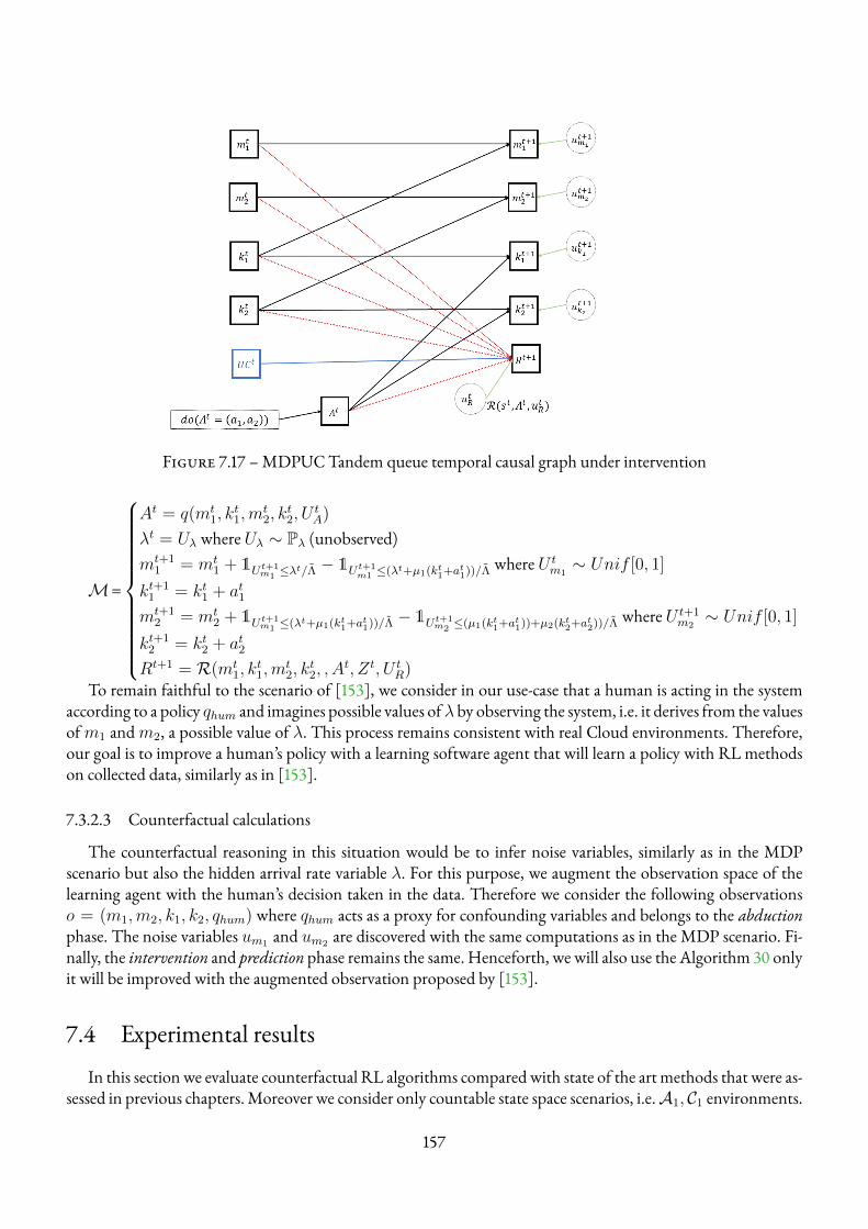
Figure 7.17 –MDPUCTandem queue temporal causal graph under intervention

M=

At = q(mt1, k

t1,m

t2, k

t2, U

tA)

λt = Uλ where Uλ ∼ Pλ (unobserved)mt+1

1 = mt1 + 1Ut+1

m1≤λt/Λ − 1Ut+1

m1 ≤(λt+µ1(kt1+at1))/Λ where U tm1∼ Unif [0, 1]

kt+11 = kt1 + at1mt+1

2 = mt2 + 1Ut+1

m1≤(λt+µ1(kt1+at1))/Λ − 1Ut+1

m2≤(µ1(kt1+at1))+µ2(kt2+at2))/Λ where U t+1

m2∼ Unif [0, 1]

kt+12 = kt2 + at2Rt+1 = R(mt

1, kt1,m

t2, k

t2, , A

t, Zt, U tR)

To remain faithful to the scenario of [153], we consider in our use-case that a human is acting in the systemaccording to a policy qhum and imagines possible values ofλ by observing the system, i.e. it derives from the valuesofm1 andm2, a possible value of λ. This process remains consistent with real Cloud environments. Therefore,our goal is to improve a human’s policy with a learning software agent that will learn a policy with RL methodson collected data, similarly as in [153].

7.3.2.3 Counterfactual calculations

The counterfactual reasoning in this situation would be to infer noise variables, similarly as in the MDPscenario but also the hidden arrival rate variable λ. For this purpose, we augment the observation space of thelearning agent with the human’s decision taken in the data. Therefore we consider the following observationso = (m1,m2, k1, k2, qhum) where qhum acts as a proxy for confounding variables and belongs to the abductionphase. The noise variables um1 and um2 are discovered with the same computations as in the MDP scenario. Fi-nally, the intervention and prediction phase remains the same. Henceforth, we will also use the Algorithm 30 onlyit will be improved with the augmented observation proposed by [153].

7.4 Experimental resultsIn this section we evaluate counterfactual RL algorithms compared with state of the art methods that were as-

sessed in previous chapters.Moreover we consider only countable state space scenarios, i.e.A1, C1 environments.

157

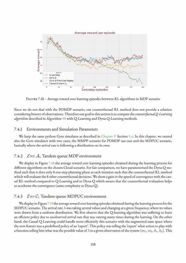
Figure 7.18 – Average reward over learning episodes between RL algorithms inMDP scenario

Since we do not deal with the POMDP scenario, our counterfactual RL method does not provide a solutionconsidering history of observations.Therefore our goal in this section is to compare the counterfactual Q-Learningalgorithm described in Algorithm 30 with Q-Learning and Dyna-Q-Learning methods.

7.4.1 Environments and Simulation ParametersWe keep the same python Gym simulator as described in Chapter V Section 5.4. In this chapter, we extend

also the Gym simulator with two cases, the MMPP scenario for POMDP use-case and the MDPUC scenario,basically where the arrival rate is following a distribution on its own.

7.4.2 EnvA1 Tandem queueMDP environmentWe display in Figure 7.18 the average reward over learning episodes obtained during the learning process for

different algorithms on the chosen Cloud scenario. For fair comparison, we have parameterised the Dyna-Qme-thod such that it does only 8 one-step planning phase at each iteration such that the counterfactual RL methodwhichwill evaluate the 8 other counterfactual decisions.We show a gain in the speed of convergence with the cau-sal RL method compared to Q-Learning and to Dyna-Q which means that the counterfactual evaluation helpsto accelerate the convergence (same complexity as Dyna-Q).

7.4.3 Env C1 Tandem queueMDPUC environmentWedisplay in Figure 7.19 the average reward over learning episodes obtainedduring the learningprocess for the

MDPUC scenario. The arrival rate λwas taking several values and changing at a given frequency, where its valueswere drawn from a uniform distribution. We first observe that the Q-learning algorithm was suffering to learnan efficient policy due to unobserved arrival rate that was varying many times during the learning. On the otherhand, the Causal Q Learning could handle more efficiently this scenario with the augmented state space wherethe new feature was a predefined policy of an ’expert’. This policy was telling the ’expert’ what action to play witha function telling himwhatwas the possible value ofλ in a given observation of the system (m1,m2, k1, k2). This

158

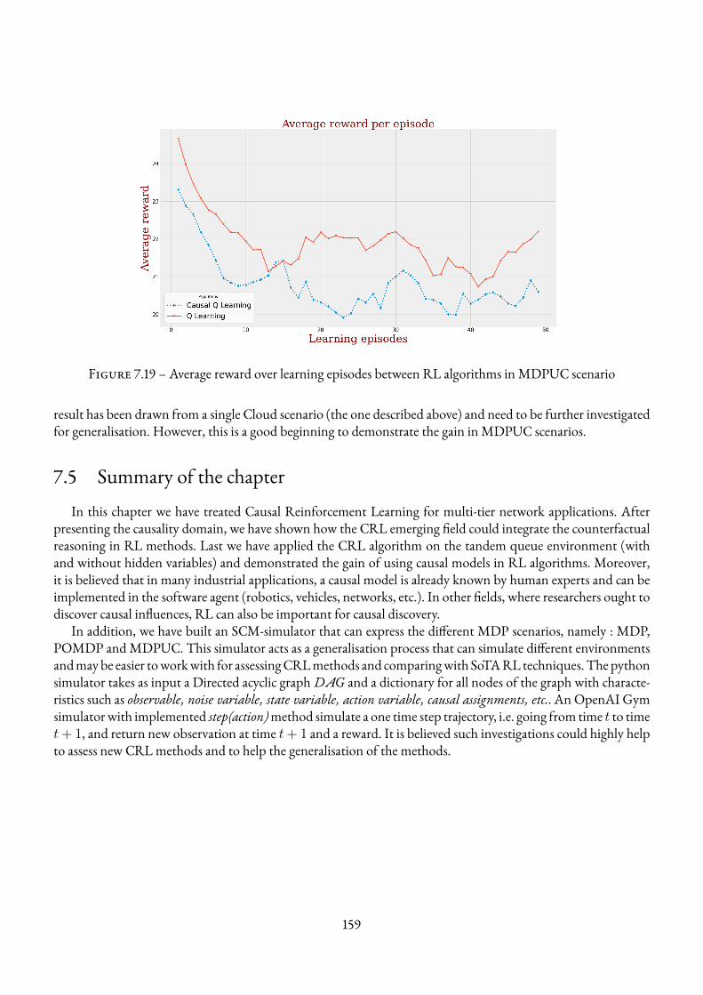
Figure 7.19 – Average reward over learning episodes between RL algorithms inMDPUC scenario

result has been drawn from a single Cloud scenario (the one described above) and need to be further investigatedfor generalisation. However, this is a good beginning to demonstrate the gain in MDPUC scenarios.

7.5 Summary of the chapterIn this chapter we have treated Causal Reinforcement Learning for multi-tier network applications. After

presenting the causality domain, we have shown how the CRL emerging field could integrate the counterfactualreasoning in RL methods. Last we have applied the CRL algorithm on the tandem queue environment (withand without hidden variables) and demonstrated the gain of using causal models in RL algorithms. Moreover,it is believed that in many industrial applications, a causal model is already known by human experts and can beimplemented in the software agent (robotics, vehicles, networks, etc.). In other fields, where researchers ought todiscover causal influences, RL can also be important for causal discovery.

In addition, we have built an SCM-simulator that can express the different MDP scenarios, namely : MDP,POMDP andMDPUC. This simulator acts as a generalisation process that can simulate different environmentsandmaybe easier toworkwith for assessingCRLmethods and comparingwith SoTARL techniques.Thepythonsimulator takes as input a Directed acyclic graphDAG and a dictionary for all nodes of the graph with characte-ristics such as observable, noise variable, state variable, action variable, causal assignments, etc.. An OpenAI Gymsimulatorwith implemented step(action)method simulate a one time step trajectory, i.e. going from time t to timet+ 1, and return new observation at time t+ 1 and a reward. It is believed such investigations could highly helpto assess new CRLmethods and to help the generalisation of the methods.

159

CHAPTER 8

DISCUSSION

In order to conclude this work, three sections are presented to summarise the contributions of the thesis andto give the resulting perspectives. The first section is a taxonomy of the Reinforcement Learning field that oughtto unified all the methods we have seen throughout this document in the different chapters. This allows us tohave a broad overview of the field. The second section presents a summary of the contributions of the thesis.It reviews the contributions of each chapter, mentioning the important points. We finish this document withthe presentation of the perspectives that derive from the different works. Here again we mention the generalperspectives of the thesis but also specific points in each chapter.

8.1 Taxonomy of the Reinforcement Learning fieldIn this section we want to characterise the different RLmethods and their behavior in different environments

with what we have seen throughout the manuscript in the different chapters (model-free RL, model-based RL,factored and causal RL). We mainly try to give a global definition to all the possible elements of the RL field :model representation, knowledge of the environment, how the agent can learn the policy or the value function.

General RL Algorithms and Agent’s KnowledgeFirst, we describe the potential knowledge the learning agent can carry and that he can think as a toolbox to

learn an optimal policy. Basically, we have twomajor domains : theMDPdomainwhere the agent knows perfectlythe environment model and can plan; and the RL domain where it has some missing information and needs tointeract for data collection.

Agent’s knowledge of the environment

First, the learning agent may have disparate understanding of the environment, i.e. different informationabout the systems statistics but also different representation of the world model.

r Markov Decision Process with full information about dynamics and reward functions :

— State-transitional modelP ,R [MDP];— Factored state-transitional model Fact(P), Fact(R) with DBNs structureD [FMDP];— Structural causal modelF ,P(U) with causal graph structure G [CMDP].

160

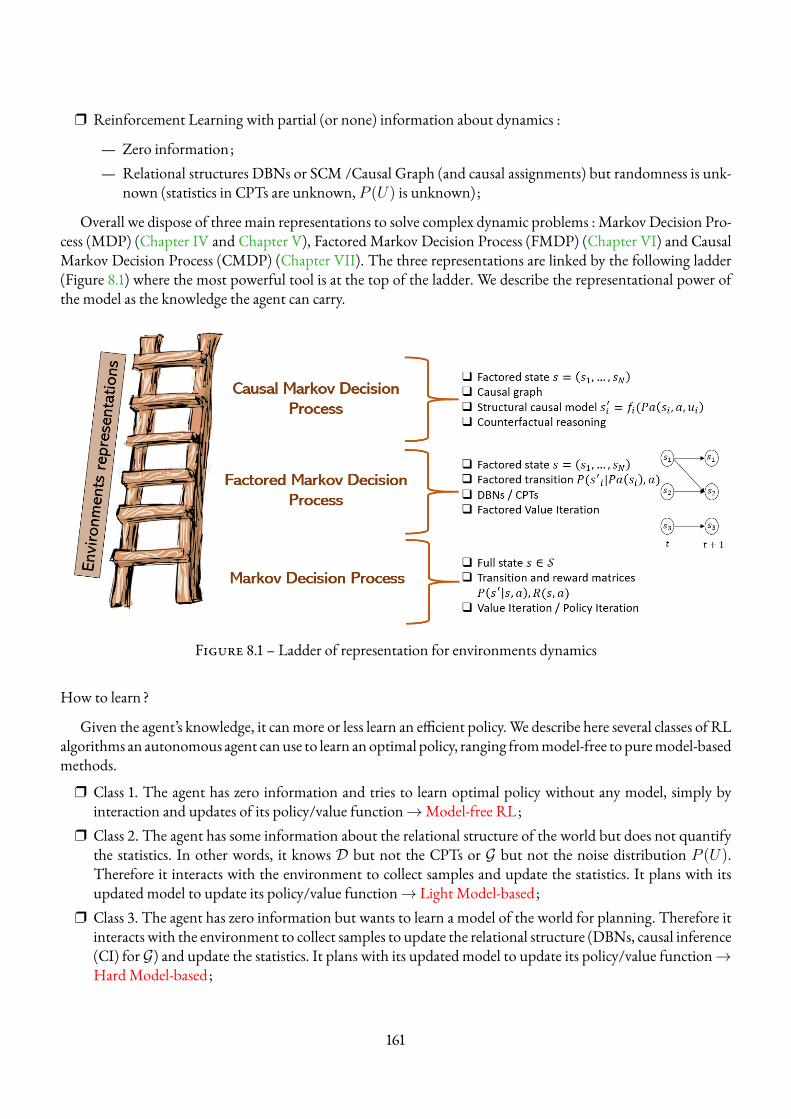
r Reinforcement Learning with partial (or none) information about dynamics :

— Zero information;— Relational structures DBNs or SCM /Causal Graph (and causal assignments) but randomness is unk-

nown (statistics in CPTs are unknown, P (U) is unknown) ;

Overall we dispose of three main representations to solve complex dynamic problems :Markov Decision Pro-cess (MDP) (Chapter IV and Chapter V), Factored Markov Decision Process (FMDP) (Chapter VI) and CausalMarkov Decision Process (CMDP) (Chapter VII). The three representations are linked by the following ladder(Figure 8.1) where the most powerful tool is at the top of the ladder. We describe the representational power ofthe model as the knowledge the agent can carry.

Figure 8.1 – Ladder of representation for environments dynamics

How to learn?

Given the agent’s knowledge, it canmore or less learn an efficient policy.We describe here several classes of RLalgorithms an autonomous agent canuse to learn anoptimal policy, ranging frommodel-free to puremodel-basedmethods.

r Class 1. The agent has zero information and tries to learn optimal policy without any model, simply byinteraction and updates of its policy/value function→Model-free RL;

r Class 2. The agent has some information about the relational structure of the world but does not quantifythe statistics. In other words, it knows D but not the CPTs or G but not the noise distribution P (U).Therefore it interacts with the environment to collect samples and update the statistics. It plans with itsupdated model to update its policy/value function→ Light Model-based;

r Class 3. The agent has zero information but wants to learn a model of the world for planning. Therefore itinteracts with the environment to collect samples to update the relational structure (DBNs, causal inference(CI) for G) and update the statistics. It plans with its updated model to update its policy/value function→HardModel-based;

161

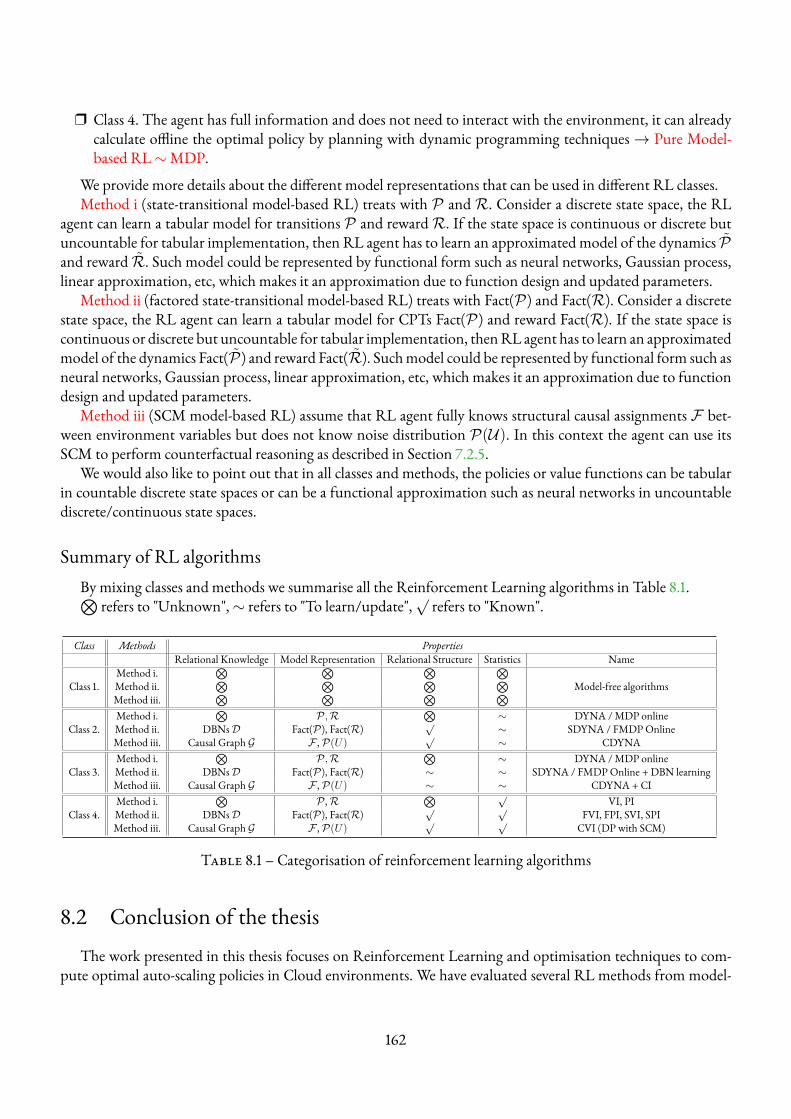
r Class 4. The agent has full information and does not need to interact with the environment, it can alreadycalculate offline the optimal policy by planning with dynamic programming techniques→ Pure Model-based RL∼MDP.

We provide more details about the different model representations that can be used in different RL classes.Method i (state-transitional model-based RL) treats with P and R. Consider a discrete state space, the RL

agent can learn a tabular model for transitions P and rewardR. If the state space is continuous or discrete butuncountable for tabular implementation, then RL agent has to learn an approximated model of the dynamics Pand reward R. Such model could be represented by functional form such as neural networks, Gaussian process,linear approximation, etc, which makes it an approximation due to function design and updated parameters.

Method ii (factored state-transitional model-based RL) treats with Fact(P) and Fact(R). Consider a discretestate space, the RL agent can learn a tabular model for CPTs Fact(P) and reward Fact(R). If the state space iscontinuous or discrete but uncountable for tabular implementation, thenRL agent has to learn an approximatedmodel of the dynamics Fact(P) and reward Fact(R). Suchmodel could be represented by functional form such asneural networks, Gaussian process, linear approximation, etc, which makes it an approximation due to functiondesign and updated parameters.

Method iii (SCM model-based RL) assume that RL agent fully knows structural causal assignments F bet-ween environment variables but does not know noise distribution P(U). In this context the agent can use itsSCM to perform counterfactual reasoning as described in Section 7.2.5.

We would also like to point out that in all classes and methods, the policies or value functions can be tabularin countable discrete state spaces or can be a functional approximation such as neural networks in uncountablediscrete/continuous state spaces.

Summary of RL algorithmsBy mixing classes and methods we summarise all the Reinforcement Learning algorithms in Table 8.1.⊗

refers to "Unknown",∼ refers to "To learn/update",√refers to "Known".

Class Methods PropertiesRelational Knowledge Model Representation Relational Structure Statistics Name

Class 1.Method i.

⊗ ⊗ ⊗ ⊗Method ii.

⊗ ⊗ ⊗ ⊗Model-free algorithms

Method iii.⊗ ⊗ ⊗ ⊗

Class 2.Method i.

⊗P ,R

⊗∼ DYNA /MDP online

Method ii. DBNsD Fact(P), Fact(R)√

∼ SDYNA / FMDPOnlineMethod iii. Causal Graph G F ,P(U)

√∼ CDYNA

Class 3.Method i.

⊗P ,R

⊗∼ DYNA /MDP online

Method ii. DBNsD Fact(P), Fact(R) ∼ ∼ SDYNA / FMDPOnline + DBN learningMethod iii. Causal Graph G F ,P(U) ∼ ∼ CDYNA + CI

Class 4.Method i.

⊗P ,R

⊗ √VI, PI

Method ii. DBNsD Fact(P), Fact(R)√ √

FVI, FPI, SVI, SPIMethod iii. Causal Graph G F ,P(U)

√ √CVI (DP with SCM)

Table 8.1 – Categorisation of reinforcement learning algorithms

8.2 Conclusion of the thesisThe work presented in this thesis focuses on Reinforcement Learning and optimisation techniques to com-

pute optimal auto-scaling policies in Cloud environments. We have evaluated several RL methods from model-

162

free tomodel-based and structural approaches in different Cloud scenarios (single physical node, multi-tier archi-tecture).

The first application (Chapter IV) where we provided the true model to the agent allows us to compare aMarkov Decision Process approach against a Markov Chain approach to compute threshold policies for Cloudresource allocation.We provided an aggregation technique to accelerate the computations of the heuristics, basedon the Markov Chain aggregation and decomposition of the cost calculations. Moreover, we studied structuralhysteresis MDP algorithms with heuristics and we showed that structural MDP algorithms were outperformingheuristics in accuracy and execution time and could handle large-scale systems. These results go against someassumptions in the literature stating that heuristics perform better. Last, we performed analysis in a real Cloudmodel demonstrating how fast the MDP techniques could compute optimal threshold rules in Cloud systems.These results also encourageCloudproviders toutilise such techniques for thresholds computations after definingconsistent queuing metrics for the reward function and after inferring arrivals distributions with traces.

Secondly, we have illustrated in Chapter V that model-based reinforcement learning could outperform stateof the art model-free techniques such as Q-Learning in a tandem queue system where the agent has to learn themodel of the world from interventional data for planning. This is noteworthy because standard RL applicationsin industrial use-cases are model-free and we believe that investing a little more in model-based techniques couldincrease the performance of RL for concrete use-cases.

Again, adding more precise knowledge to the learning agent with structural representation of the environ-ment model (factored and causal), demonstrated that this supplementary information provided to the agent washelping him to obtain better performance. This was shown in the factored approach in Chapter VI (assumingthat the environment is consistent with this approach) where more compact representation of the environmentmodel could lead to better performance by highly reducing the complexity of algorithms.We believe that this fra-mework should also be deeper investigated in industrial applications where environments permits its utilisation(end-to-end scenarios with local relations : robotics, logistics, networks, etc.).

In addition, the causal reasoning (Chapter VII) can bring benefits in scenarios with hidden variables which isoften the case in practice in industrial applications. Although the field CRL is new and emerging, there is a highinterest to investigate in such solutions (theoretically and practically) to democratise CRL in real use-cases. Onthe other hand, it is believed that causal relationships are intrinsically in nature and that this can be applied in allfields.

8.3 Perspectives of the thesisThis thesis makes the link between model-based reinforcement learning algorithms and the search of auto-

scaling policies in Cloud environments. In this section, we provide some directions to deepen our work, in eachof the following areas that were cover in the document.

Cloud environmentsFirst, the consideration ofmore complexCloud environments is crucial to evaluate the learning of auto-scaling

policies. In this document we have investigated two main applications : a single physical node hosting virtualresources and a multi-tier Cloud network with two physical nodes in tandem. To have a deeper evaluation andcomparison of RLmethods, it is crucial to consider more complex networks ; e.g. multi-tier networks with manynodes in tandem or general networks. This could also raise interest to demonstrate the gain of factored and causalapproaches inmore complexCloud structures. In addition to increasing the complexity ofCloud infrastructure, itmay also be interesting to considermore complexqueueingmodelswith general arrivals distributions and services,

163

with load balancing process, etc. This can be achieved through more complex queueing modelling for Cloudenvironments representation, for example by looking at the literature or at the behavior of real Cloud platforms.

Simulations and real platform evaluationSecondly, all our assessments and comparison were made in simulated environments : python simulator for

Reinforcement Learning studies and computational software for the treatment of MDP versus heuristics. Togive more strength to our work, one major outlook is to evaluate all the investigations in real Cloud platforms.This could be done in experimental Docker platforms developed with Kubernetes or Openstack for example.Moreover, hysteresis and thresholds rules could be evaluated in real Cloud platform such as AwS EC2 or Azure.

Theoretical extensionsFinally, we mentioned throughout this document, mostly during the summary of the chapters, the improve-

ment that could bemade regarding theRL algorithms and their comparison.We aggregate here what can be donein each chapter.

Model-based Reinforcement Learning

The work presented in the chapter Chapter V requires deeper comparison and set of parameters to evaluatemore globally the considered RL algorithms in Cloud environments. We also want to consider larger-scale sce-narios where we might have to approximate policy, value function or models with functional forms such as neu-ral networks, linear approximations, Gaussian processes, etc. Moreover, it could be interesting to investigate thestructural form of the optimal policies in the tandem queue environment. This could lead us to integrate thisstructural properties in the Reinforcement Learning algorithms to speed up the convergence such as in ChapterIV.

Factored Reinforcement Learning

Equally, the factored approach (Chapter VI) should be further evaluated. This should be done by consideringlarger set of parameters for the simulations, but alsomore complexCloudnetworks.One other path is to comparein very large scale environments the performance of our FMDP online method compared with state of the artDeepRLmethods such asDQNor PPO for example.Moreover, we decided in this document towork on tabularrepresentation of the local factored transition probabilities. It can also be of great interest to tackle the problemwith decision tree and decision diagram representations.

Causal Reinforcement Learning

For the causal approach many paths can be considered. First on the algorithmic domain there are several ele-ments to investigate regarding the counterfactual reasoning process for differentMDP environments (MDPUC,POMDP, etc.). Secondly, there may be an interesting work to be explored regarding the connection betweenfactored and causal approaches, i.e. the relations between DBN and Causal Graph representations. In addition,there is still a lot of evaluation to do for causal methods, in particular with the treatment of partially observableenvironments with the consideration of historical data.

164

Hierarchical framework

Finally, one orthogonal approach that was not presented in this document is the hierarchical framework. Thegeneral idea of hierarchical MDPmethods is to split the state space into subsets of limited size, compute the localoptimal policies for each subset, and then combine these policies to obtain an optimal policy on the on the globalMDP. These techniques are related with the aggregation we studied in Chapter IV. The idea is similar in that itsgoal is to accelerate the convergence by diminishing the dimension of the problem in smaller sub MDPs easierto solve. Moreover, Guestrin et al. studied the intersection between factored and hierarchical MDP with LinearProgramming [50]. Kozolava [83] also investigated both approaches and this is one path that could be followedregarding the Chapter VI.

165

REFERENCES

Book Sources[1] I.Goodfellow, Y. Bengio et A. Courville. Deep Learning. MIT Press, 2016. url :

http://www.deeplearningbook.org.[2] G. Pdmia. Markov Decision Processes In Artificial Intelligence. JohnWiley & Sons, Inc., 2013. doi :

10.1002/9781118557426.[3] J. Pearl. Causality - Models, Reasoning and Inference. 2nd. Cambridge University Press, 2009.[4] W. B. Powell. Approximate Dynamic Programming. Solving the Curses of Dimensionality. Sous la

dir. de J.Wiley et Sons. 2011.[5] M. Puterman. Markov Decision Processes - Discrete Stochastic Dynamic Programming. Wiley, 1994.

doi : 10.1002/9780470316887.[6] D.-P. Song. Optimal Control and Optimization of Stochastic Supply Chain Systems. Springer-Verlag,

2013. doi : 10.1007/978-1-4471-4724-4.[7] W. Stewart. Introduction to the Numerical Solution of Markov Chains. Princeton, University Press,

1994.[8] R. Sutton et A. Barto. Reinforcement Learning - An Introduction. TheMIT press, 2015.[9] J.Teghem. Recherche opérationnelle - Tome 1. T. 1. Ellipse, 2013.

Conference and Journal papers[10] I.Adan, V.Kulkarni et A. vanWijk. «Optimal Control of a Server Farm». In :

Information Systems and Operational Research 51.4 (2013), p. 241–252. doi :10.3138/infor.51.4.241.

[11] I.Alam et al.«A Survey of Network Virtualization Techniques for Internet of Things Using SDNand NFV». In : ACMComput. Surv. 53.2 (2020). doi : 10.1145/3379444.

[12] A.Ali-Eldin et al. « Efficient Provisioning of Bursty Scientific Workloads on the Cloud UsingAdaptive Elasticity Control ». In : 3rdWorkshop on Scientific Cloud Computing (2012).

[13] Amazon. Amazon EC2 Pricing. 2019. url : https://aws.amazon.com/fr/ec2/pricing/.

166

[14] Amazon. AWS Auto Scaling. 2018. url : http://aws.amazon.com/autoscaling/.[15] Amazon. AWS Serverless Multi-Tier Architectures. AWSWhitepaper. 2019. url : https:

//d0.awsstatic.com/whitepapers/AWS_Serverless_Multi-Tier_Architectures.pdf.[16] D.Ardagna et al. «Quality-of-service in cloud computing : modeling techniques and their

applications». In : Journal of Internet Services and Applications 5 (2014). doi :10.1186/s13174-014-0011-3.

[17] J.Artalejo, A. Economou et M. Lopez-Herrero. «Analysis of a multiserver queue with setuptimes». In : Queueing Systems 51.1-2 (2005), p. 53–76. doi : 10.1007/s11134-005-1740-6.

[18] N.Asghari, M.Mandjes et A.Walid. « Energy-efficient scheduling in multi-core servers ». In :Computer Networks 59.11 (2014), p. 33–43. doi : 10.1016/j.bjp.2013.12.009.

[19] D. Bacigalupo et al. «Resource management of enterprise cloud systems using layered queuing andhistorical performance models ». In :Proceedings of the 2010 IEEE International Symposium on Parallel and Distributed Processing (2010).doi : 10.1109/IPDPSW.2010.5470782.

[20] E. Bareinboim et al. «On Pearl’s Hierarchy and the Foundations of Causal Inference». In :Technical Report (2021). url : https://causalai.net/r60.pdf.

[21] E. Barrett, E.Howley et J.Duggan. «A learning architecture for scheduling workflowapplications in the cloud». In : European Conference onWeb Services. 2011, p. 83–90. doi :10.1109/ECOWS.2011.27.

[22] E. Barrett, E.Howley et J.Duggan. «Applying reinforcement learning towards automatingresource allocation and application scalability in the cloud». In :Concurrency and Computation - Practice and Experience 25.12 (2013), p. 1656–1674. doi :https://doi.org/10.1002/cpe.2864.

[23] A. G. Barto, S. J. Bradtke et S. Singh. « Learning to Act Using Real-Time DynamicProgramming». In : Artif. Intell. 72 (1995), p. 81–138.

[24] C. Belady et al. «Green grid data center power efficiency metrics : PUE and DCIE». In : 2008.[25] A. Benoit et al. «Reducing the energy consumption of large scale computing systems through

combined shutdown policies with multiple constraints ». In : Int. J. High Perform. Comput. Appl. 32.1(2018), p. 176–188. doi : 10.1177/1094342017714530.

[26] C. Boutilier, R.Dearden et M.Goldszmidt. « Stochastic dynamic programming with factoredrepresentations». In : Artificial Intelligence 121 (2000), p. 49–107. doi :10.1016/S0004-3702(00)00033-3.

[27] R. Brafman et M.Tennenholtz. «R-Max - A General Polynomial Time Algorithm fornear-Optimal Reinforcement Learning». In : J. Mach. Learn. Res. 3 (2003), p. 213–231. doi :10.1162/153244303765208377.

[28] M. Braglia et al. «A continuous review, (Q, r) inventory model for a deteriorating item with randomdemand and positive lead time». In : Computers and Operations Research 109 (2019), p. 102–121.doi : 10.1016/j.cor.2019.04.019.

[29] G. Brockman et al.«Openai gym». In : CoRR abs/1606.01540 (2016). arXiv : 1606.01540.[30] L. Buesing et al. «Woulda, Coulda, Shoulda : Counterfactually-Guided Policy Search». In : CoRR

abs/1811.06272 (2018). arXiv : 1811.06272.

167

[31] J. Cao et al. «Web Server Performance Modeling using anM/G/1/K*PS Queue». In :10th International Conference on Telecommunications (2003), p. 1501–1506. doi :10.1109/ICTEL.2003.1191656.

[32] E. Casalicchio et L. Silvestri. «Autonomic Management of Cloud-Based Systems : The ServiceProvider Perspective ». In : Springer London, 2013, p. 39–47. doi :10.1007/978-1-4471-4594-3_5.

[33] T. Chieu et al. «Dynamic Scaling of Web Applications in a Virtualized Cloud ComputingEnvironment». In : nov. 2009, p. 281–286. doi : 10.1109/ICEBE.2009.45.

[34] C. Colas, O. Sigaud et P.-Y.Oudeyer.A Hitchhiker’s Guide to Statistical Comparisons of Reinforcement Learning Algorithms. 2019. arXiv :1904.06979.

[35] T.Degris, O. Sigaud et P.-H.Wuillemin. « Learning the Structure of FactoredMarkov DecisionProcesses in Reinforcement Learning Problems». In :23rd International Conference onMachine Learning (2006). doi : 10.1145/1143844.1143877.

[36] M.Deisenroth et C.Rasmussen. « PILCO : AModel-Based and Data-Efficient Approach to PolicySearch. » In : jan. 2011, p. 465–472.

[37] G.Ducamp, C.Gonzales et P.-H.Wuillemin. « aGrUM/pyAgrum : a Toolbox to Build Modelsand Algorithms for Probabilistic Graphical Models in Python». In :10th International Conference on Probabilistic Graphical Models. T. 138. Proceedings of MachineLearning Research. Skørping, Denmark, sept. 2020, p. 609–612. url :https://hal.archives-ouvertes.fr/hal-03135721.

[38] X.Dutreilh et al.«Using Reinforcement Learning for Autonomic Resource Allocation in Clouds :Towards a Fully AutomatedWorkflow». In : ICAS (2011).

[39] X.Dutreilh et al. « FromData Center Resource Allocation to Control Theory and Back». In :IEEE 3rd International Conference on Cloud Computing (2010), p. 410–417.

[40] T. Ercan et B. Yusuf. «An Efficient QueuingModel for Resource Sharing in Cloud Computing».In : The International Journal of Engineering and Science 3 (oct. 2014), p. 36–43.

[41] K. R. Evangelin et V.Vidhya. « Performance Measures of QueuingModels Using CloudComputing». In : Asian Journal of Engineering and Applied Technology 4 (2015), p. 8–11.

[42] A. Federgruen et C. So. «Optimality of threshold policies in single-server queueing systems withserver vacations». In : Advances in Applied Probability 23.2 (1991), p. 388–405. doi :10.2307/1427755.

[43] W. Fedus et al. «Revisiting Fundamentals of Experience Replay». In : 2020.[44] V. Feinberg et al. «Model-Based Value Estimation for Efficient Model-Free Reinforcement

Learning». In : ArXiv abs/1803.00101 (2018).[45] A.Gandhi, M.Harchol-Balter et I.Adan. « Server farms with setup costs ». In :

Performance Evaluation 67.11 (2010), p. 1123–1138. doi : 10.1016/j.peva.2010.07.004.[46] Y.Gari et al. «Reinforcement Learning-based Application Autoscaling in the Cloud : A Survey». In :

Engineering Applications of Artificial Intelligence 102 (2021). doi :10.1016/j.engappai.2021.104288.

[47] S.Gershman. «Reinforcement learning and causal models ». In : (2015).

168

[48] H.Ghanbari et al. « Exploring Alternative Approaches to Implement an Elasticity Policy ». In :Proceedings of the 2011 IEEE 4th International Conference on Cloud Computing. CLOUD ’11. IEEEComputer Society, 2011, p. 716–723. doi : 10.1109/CLOUD.2011.101.

[49] E.Ghomi, A.Rahmani et N.Qader. «Applying queue theory for modeling of cloud computing : Asystematic review». In : Concurrency and Computation, Practice and Experience 31.17 (2019). doi :https://doi.org/10.1002/cpe.5186.

[50] C.Guestrin, R. Parr et S.Venkataraman. « Efficient solution algorithms for factoredMDPs».In : Journal of Artificial Intelligence Research 19 (2003), p. 399–468.

[51] C.Guestrin, R. Patrascu et D. Schuurmans. «Algorithm-Directed Exploration for Model-BasedReinforcement Learning in FactoredMDPs». In : ICML. 2002.

[52] L.Guo et al. «Dynamic Performance Optimization for Cloud Computing UsingM/M/mQueueingSystem». In : Journal of applied mathematics (2014). doi : 10.1155/2014/756592.

[53] S.Gupta et A. Sakshi. «Queuing systems in cloud services management : A survey». In :International Journal of Pure and Applied Mathematics 119 (jan. 2018), p. 12741–12753.

[54] D.Guyon et al. « Involving Users in Energy Conservation : A Case Study in Scientific Clouds». In :International Journal of Grid and Utility Computing, Inderscience (2018), p. 1–14. doi :10.1504/IJGUC.2019.10021321.

[55] T.Haarnoja et al. « Soft Actor-Critic : Off-Policy Maximum Entropy Deep Reinforcement Learningwith a Stochastic Actor ». In : 2018.

[56] H. V.Hasselt, M.Hessel et J.Aslanides. «When to use parametric models in reinforcementlearning?» In : NeurIPS. 2019.

[57] M.Hessel et al.«Rainbow : Combining Improvements in Deep Reinforcement Learning». In :The 32nd AAAI Conference on Artificial Intelligence (2017). url :https://ojs.aaai.org/index.php/AAAI/article/view/11796.

[58] S.Hipp et U.Holzbaur. «Decision Processes with Monotone Hysteretic Policies ». In :Operations Research 36.4 (1988), p. 585–588. url : https://www.jstor.org/stable/171138.

[59] J.Hoey et al. « SPUDD : Stochastic planning using decision diagrams». In :Uncertainty in Aritificial Intelligence (1999), p. 279–288. url :https://dl.acm.org/doi/10.5555/2073796.2073828.

[60] G.Holland, E.Talvitie et M. Bowling. «The Effect of Planning Shape on Dyna-style Planning inHigh-dimensional State Spaces ». In : (juin 2018).

[61] S.Horovitz et Y.Arian. « Efficient cloud auto-scaling with SLAObjective Using Q-Learning». In :IEEE FiCloud. 2018. doi : 10.1109/FiCloud.2018.00020.

[62] E.Hyon et A. Jean-Marie. «Optimal control of admission in service in a queue with impatience andsetup costs ». In : Performance Evaluation 144 (2020), p. 102134. issn : 0166-5316. doi :https://doi.org/10.1016/j.peva.2020.102134.

[63] O. Ibe et J.Keilson. «Multi-server threshold queues with hysteresis ». In : Performance Evaluation 21(1995), p. 185–213. doi : 10.1016/0166-5316(94)E0043-I.

[64] N. Jain et S. Choudhary. «Overview of virtualization in cloud computing». In : 2016, p. 1–4. doi :10.1109/CDAN.2016.7570950.

169

[65] V. Jain, S.Qi et K.Ramakrishnan. « Fast Function Instantiation with Alternate VirtualizationApproaches ». In :2021 IEEE International Symposium on Local andMetropolitan Area Networks (LANMAN). 2021,p. 1–6. doi : 10.1109/LANMAN52105.2021.9478808.

[66] A. Jean-Marie. «marmoteCore : a MarkovModeling Platform». In : VALUETOOLS. 2017,p. 60–65. doi : 10.1145/3150928.3150960.

[67] L. Jianyong et Z.Xiaobo. «On Average Reward Semi-Markov Decision Processes with a GeneralMultichain Structure ». In : Mathematics of Operations Research 29 (2004), p. 339–352.

[68] Y. Jin et al.«Testing a Q-learning Approach for Derivation of Scaling Policies in Cloud-basedApplications». In : ICIN. 2018. doi : 10.1109/ICIN.2018.8401621.

[69] S.Kakade. «On the Sample Complexity of Reinforcement Learning». Thèse de doct. 2003.[70] G.Kalweit et J. Boedecker. «Uncertainty-driven Imagination for Continuous Deep

Reinforcement Learning». In : Proceedings of the 1st Annual Conference on Robot Learning 78(2017), p. 195–206. url : https://proceedings.mlr.press/v78/kalweit17a.html.

[71] M.M.Kandi et al. «Analysis of Performance and Energy Consumption in the Cloud». In :Computer Performance Engineering - 14th EuropeanWorkshop, EPEW. 2017, p. 199–213. doi :10.1007/978-3-319-66583-2_13.

[72] A.Kansal et al.«Virtual Machine Power Metering and Provisioning». In :ACM Symposium on Cloud Computing (2010), p. 39–50.

[73] M.Kearns et D.Koller. « Efficient Reinforcement Learning in FactoredMDPs». In :Proceedings of the 16th International Joint Conference on Artificial Intelligence - Volume 2. IJCAI’99.Stockholm, Sweden : Morgan Kaufmann Publishers Inc., 1999, p. 740–747. url :https://dl.acm.org/doi/10.5555/1624312.1624325.

[74] M.Kearns et S. Singh. «Near-Optimal Reinforcement Learning in Polynomial Time». In :Machine Learning 49 (2002), p. 209–232. doi : 10.1023/A:1017984413808.

[75] D.Kenga, V. O.Omwenga et P. J.Ogao. «AMethod for Measuring Energy Consumption in IaaSCloud». In : JACET (2020).

[76] A. A.Khan, M. Zakarya et R.Khan. « Energy-aware dynamic resource management in elastic clouddatacenters ». In : SimulationModelling Practice and Theory 92 (2019), p. 82–99.

[77] G.Kibalya et al. «A Reinforcement Learning Based Approach for 5GNetwork Slicing AcrossMultiple Domains ». In :2019 15th International Conference on Network and Service Management (CNSM). 2019, p. 1–5. doi :10.23919/CNSM46954.2019.9012674.

[78] M.Kitaev et R. Serfozo. «M/M/1Queues with Switching Costs andHysteretic Optimal Control ».In : Operations Research 47 (1999), p. 310–312. url : https://www.jstor.org/stable/223048.

[79] D.Koller et R. Parr. « Policy Iteration for FactoredMDPs». In : UAI’00 (2000), p. 326–334. url :https://dl.acm.org/doi/10.5555/2073946.2073985.

[80] J.Koo et al. «Deep Reinforcement Learning for Network Slicing with Heterogeneous ResourceRequirements and Time Varying Traffic Dynamics ». In :2019 15th International Conference on Network and Service Management (CNSM). 2019, p. 1–5. doi :10.23919/CNSM46954.2019.9012702.

170

[81] G.Koole. «A simple proof of the optimality of a threshold policy in a two-server queueing system».In : Systems and Control Letters 26 (1995), p. 301–303. doi : 10.1016/0167-6911(95)00015-1.

[82] P.Koperek et F.Wlodzimierz. «Dynamic Business Metrics-driven Resource Provisioning in CloudEnvironments ». In : (2012), p. 171–180. doi : 10.1007/978-3-642-31500-8_18.

[83] O.Kozlova. «Hierarchical and factored reinforcement learning». Thèse de doct. 2010. url :https://tel.archives-ouvertes.fr/tel-00632968/document.

[84] A.Kranenburg et G. vanHoutum. «Cost optimization in the (S-1, S) lost sales inventory modelwith multiple demand classes ». In : Oper. Res. Lett. 35.4 (2007), p. 493–502. doi :10.1016/j.orl.2006.04.004.

[85] B.Krishnan et al. «VM Power Metering : Feasibility and Challenges ». In :ACM SIGMETRICS Performance Evaluation Review 38 (2011), p. 56–60.

[86] J.Krzywda et al. « Power-performance tradeoffs in data center servers : DVFS, CPU Pinning,horizontal and vertical scaling». In : Future Generation Computer Systems (2018), p. 114–128. doi :10.1016/j.future.2017.10.044.

[87] M.Kurpicz, A.-C.Orgerie et A. Sobe. «Howmuch does a VM cost? Energy-proportionalAccounting in VM-based Environments ». In :Euromicro International Conference on Parallel, Distributed, and Network-Based Processing (2016).doi : 10.1109/PDP.2016.70.

[88] T. Labidi, A.Mtibaa et H. Brabra. «CSLAOnto : A Comprehensive Ontological SLAModel inCloud Computing». In : Journal on Data Semantics 5 (2016), p. 179–193. doi :10.1007/s13740-016-0070-7.

[89] G. V. Lakshmi et C. Bindhu. «AQueuingModel To Improve Quality Service by ReducingWaitingTime in Cloud». In : International Journal of Soft Computing and Engineering 4 (2014).

[90] N. Lee et V. G.Kulkarni. «Optimal Arrival Rate and Service Rate Control ofMulti-server Queues».In : Queueing Syst. Theory Appl. 76.1 (2014), p. 37–50. doi : 10.1007/s11134-012-9341-7.

[91] Q.-L. Li et al. «An Overview for Markov Decision Processes in Queues and Networks ». In :Stochastic Models in Reliability, Network Security and System Safety (oct. 2019), p. 44–71. doi :10.1007/978-981-15-0864-6_3.

[92] T. P. Lillicrap et al. «Continuous control with deep reinforcement learning». In : CoRRabs/1509.02971 (2016).

[93] X. Liu, J.Heo et L. Sha. «Modeling 3-tieredWeb applications». In : (2005), p. 307–310. doi :10.1109/MASCOTS.2005.40.

[94] Z. Liu, W.Deng et G. Chen. «Analysis of the Optimal Resource Allocation for a TandemQueueingSystem». In : Mathematical Problems in Engineering (2017). doi : 10.1155/2017/5964272.

[95] T. Lorido-Botran, J.Miguel-Alonso et J. Lozano. «A Review of Auto-scaling Techniques forElastic Applications in Cloud Environments ». In : J. Grid Computing 12 (2014), p. 559–592. doi :10.1007/s10723-014-9314-7.

[96] C. Lu. «Causal Reinforcement Learning : A Road to Artificial General Intelligence». In :Nokia Bell Labs (2019).

[97] C. Lu, B. Schölkopf et J. M.Hernández-Lobato. «Deconfounding Reinforcement Learning inObservational Settings ». In : ArXiv abs/1812.10576 (2018).

171

[98] J. C. S. Lui et L.Golubchik. « Stochastic complement analysis of multi-server threshold queues withhysteresis ». In : Performance Evaluation 35 (1 1999), p. 19–48. doi :10.1016/S0166-5316(98)00043-1.

[99] V.Maccio et D.Down. « Structural properties and exact analysis of energy-aware multiserverqueueing systems with setup times». In : Performance Evaluation 121-122 (2018), p. 48–66.

[100] J.Magnan. «Représentations graphiques de fonctions et processus décisionnels Markoviens factorisés. » PhD thesis. Université Pierre et Marie Curie - Paris VI, fév. 2016. url :https://tel.archives-ouvertes.fr/tel-01363858.

[101] M.Mao et M.Humphrey. «A Performance Study on the VM Startup Time in the Cloud». In :2012 IEEE Fifth International Conference on Cloud Computing. 2012, p. 423–430. doi :10.1109/CLOUD.2012.103.

[102] T.Mastelic et I. Brandic. «Recent Trends in Energy-Efficient Cloud Computing». In :IEEE Cloud Computing 2 (2015), p. 40–47. doi : 10.1109/MCC.2015.15.

[103] I.Mitrani. «Managing performance and power consumption in a server farm». In :Annals of Operations Research 202.1 (2013), p. 121–134. doi : 10.1007/s10479-011-0932-1.

[104] V.Mnih et al. «Asynchronous Methods for Deep Reinforcement Learning». In : ICML. 2016.[105] V.Mnih et al. «Human-level control through deep reinforcement learning». In : Nature 518 (2015),

p. 529–533. doi : 10.1038/nature14236.[106] T.Moerland, J. Broekens et C. Jonker. «Model-based Reinforcement Learning : A Survey». In :

CoRR abs/2006.16712v3 (2021). arXiv : 2006.16712v3. url :http://arxiv.org/abs/2006.16712v3.

[107] R. K.Murugesan, C. Elango et S.Kannan. «Resource Allocation in Cloud Computing withM/G/s- Queueing System». In : 2014.

[108] A.Nagabandi et al. «Neural Network Dynamics for Model-Based Deep Reinforcement LearningwithModel-Free Fine-Tuning». In :2018 IEEE International Conference on Robotics and Automation (2018), p. 7559–7566.

[109] V.Ngo. Model-based reinforcement learning. url : https://ipvs.informatik.uni-stuttgart.de/mlr/wp-content/uploads/2015/06/06-ModelBased.pdf.

[110] J.Niño-Mora. «Resource allocation and routing in parallel multi-server queues with abandonmentsfor cloud profit maximization». In : Computers and Operations Research 103 (2019), p. 221–236. doi :10.1016/j.cor.2018.11.012.

[111] L.-M. L.Ny et B.Tuffin. «A simple analysis of heterogeneous multi-server threshold queues withhysteresis ». In : 2002.

[112] H.Okamura, S.Miyata et T.Dohi. «AMarkov Decision Process Approach to Dynamic PowerManagement in a Cluster System». In : IEEE Access 3 (2015), p. 3039–3047.

[113] «Optimal resource allocation with deep reinforcement learning and greedy adaptive firefly algorithm incloud computing». In : Concurrency and Computation 34 (2022). doi : 10.1002/cpe.6657.

[114] J. Peters, D. Janzing et B. Schölkopf. « Elements of Causal Inference : Foundations and LearningAlgorithms». In : 2017.

[115] P. Poupart. «Model-based RL, Lesson». In : University of Waterloo (2018).

172

[116] C.Qu, R. Calheiros et R. Buyya. «Auto-ScalingWeb Applications in Clouds : A Taxonomy andSurvey». In : ACMComput. Surv. 73.4 (juil. 2018). doi : 10.1145/3148149.

[117] I.Rais et al. «Quantifying the Impact of Shutdown Techniques for Energy-Efficient Data Centers ».In : Concurrency and Computation - Practice and Experience 30.17 (2018), p. 1–13.

[118] A.Randa et al. «Heuristic methods for the capacitated stochastic lot-sizing problem under thestatic-dynamic uncertainty strategy». In : Computers and Operations Research 109 (2019), p. 89–101.doi : 10.1016/j.cor.2019.03.007.

[119] J.Rao et al. «VCONF - A Reinforcement Learning Approach to Virtual MachinesAuto-Configuration». In : ICAC ’09 (2009), p. 137–146. doi : 10.1145/1555228.1555263.

[120] T. Salah et al. « Performance comparison between container-based and VM-based services ». In :2017 20th Conference on Innovations in Clouds, Internet and Networks (ICIN). 2017, p. 185–190.doi : 10.1109/ICIN.2017.7899408.

[121] S. Saxena, M.Khan et R. Singh. «An Energy Saving Approach from Cloud Resources for GreenCloud Environment». In :2021 10th International Conference on SystemModeling Advancement in Research Trends (SMART).2021, p. 628–632. doi : 10.1109/SMART52563.2021.9676249.

[122] T. Schaul et al. Prioritized Experience Replay. 2016. arXiv : 1511.05952v4.[123] J. Schulman et al. « Proximal Policy Optimization Algorithms». In : ArXiv abs/1707.06347 (2017).[124] V. Sciancalepore, X. Costa-Perez et A. Banchs. «RL-NSB : Reinforcement Learning-Based 5G

Network Slice Broker ». In : IEEE Transactions on Networking 27.4 (2019), p. 1543–1557. doi :10.1109/TNET.2019.2924471.

[125] S. Scott et P. Smyth. «TheMarkovModulated Poisson Process andMarkov Poisson Cascade withApplications toWeb Traffic Modeling». In : Bayesian Statistics 7 (2003).

[126] D. Serrano et al. « SLA guarantees for cloud services ». In : Future Generation Computer Systems 54(2016), p. 233–246. doi : https://doi.org/10.1016/j.future.2015.03.018.

[127] S. Shorgin et al. «Threshold-based queuing system for performance analysis of cloud computingsystem with dynamic scaling». In : AIP Conference Proceedings 1648.1 (2015). doi :10.1063/1.4912509.

[128] G. Siddesh et K. Srinivasa. « SLA - Driven Dynamic Resource Allocation on Clouds». In :Advanced Computing, Networking and Security. Springer Berlin Heidelberg, 2012, p. 9–18.

[129] D. Silver et al. «A general reinforcement learning algorithm that masters chess, shogi, and Go throughself-play». In : Science 362.6419 (2018), p. 1140–1144. doi : 10.1126/science.aar6404.

[130] P. Singh et al. «Research on Auto-Scaling of Web Applications in Cloud : Survey, Trends and FutureDirections». In : Scalable Computing Practice and Experience 20 (2019). doi :10.12694/scpe.v20i2.1537.

[131] A. L. Strehl. «Model-Based Reinforcement Learning in Factored-State MDPs». In :2007 IEEE International Symposium on Approximate Dynamic Programming and Reinforcement Learning.2007, p. 103–110. doi : 10.1109/ADPRL.2007.368176.

[132] A. L. Strehl, C.Diuk et M. L. Littman. « Efficient Structure Learning in Factored-State MDPs».In : (2007).

173

[133] R. S. Sutton. «Dyna, an integrated architecture for learning, planning, and reacting». In :SIGART Bull 2 (1991), p. 160–163.

[134] D. Szarkowicz et T.Knowles. «Optimal Control of anM/M/S Queueing System». In :Operations Research 33.3 (1985), p. 644–660.

[135] I. Szita et A. Lörincz. « Factored Value Iteration Converges ». In : Acta Cybernetica 18 (2008),p. 615–635. url : https://dl.acm.org/doi/10.5555/1515867.1515873.

[136] I. Szita et C. Szepesvári. «Model-based reinforcement learning with nearly tight explorationcomplexity bounds». In : ICML. 2010, p. 1031–1038. url :https://icml.cc/Conferences/2010/papers/546.pdf.

[137] J.Teghem. «Control of the service process in a queueing system». In : EJOR 23.2 (1986), p. 141–158.doi : 10.1016/0377-2217(86)90234-1.

[138] G.Tesauro et al. «AHybrid Reinforcement Learning Approach to Autonomic ResourceAllocation». In : Proceedings of the 2006 IEEE International Conference on Autonomic Computing.ICAC ’06. IEEE Computer Society, 2006, p. 65–73. doi : 10.1109/ICAC.2006.1662383.

[139] T.Tournaire, H. Castel-Taleb et E.Hyon. «Optimal control policies for resource allocation inthe Cloud : comparison betweenMarkov decision process and heuristic approaches ». In : CoRRabs/2104.14879 (2021). url : https://arxiv.org/abs/2104.14879.

[140] T.Tournaire et al. « Factored Reinforcement Learning for Auto-scaling in TandemQueues ». In :NOMS 2022 - Full and short papers (). Avr. 2022. url : http://XXXXX/220997.pdf.

[141] T.Tournaire et al. «Generating optimal thresholds in a hysteresis queue : a cloud application». In :IEEEMascots. 2019. doi : 10.1109/MASCOTS.2019.00040.

[142] T.Tournaire et al. «Reinforcement Learning withModel-Based Approaches for Dynamic ResourceAllocation in a TandemQueue». In : (2021), p. 243–263. doi : 10.1007/978-3-030-91825-5_15.

[143] B.Urgaonkar et al. «An Analytical Model for Multi-Tier Internet Services and Its Applications».In : ACM SIGMETRICS Performance Evaluation Review (2005). doi :10.1145/1064212.1064252.

[144] B.Urgaonkar et al. «Dynamic Provisioning of Multi-Tier Internet Applications». In :Second International Conference on Autonomic Computing (2005), p. 217–228. doi :10.1109/ICAC.2005.27.

[145] J.Wang, A.Hertzmann et D. Fleet. «Gaussian process dynamical models ». In :Advances in neural information processing systems (2006), p. 1441–1448.

[146] D.Warsing, W.Wangwatcharakul et R.King. «Computing optimal base-stock levels for aninventory system with imperfect supply». In : Computers and Operations Research 40 (2013),p. 2786–2800. doi : 10.1016/j.cor.2013.04.001.

[147] C.Watkins et P.Dayan. «Q-Learning». In : Machine Learning 8 (1992), p. 279–292. doi :10.1007/BF00992698.

[148] Y.Wei et al. «A Reinforcement Learning Based Auto-Scaling Approach for SaaS Providers in DynamicCloud Environment». In : Mathematical Problems in Engineering 2019 (fév. 2019), p. 1–11. doi :10.1155/2019/5080647.

[149] C.-H.Wu et al. «Optimization analysis of an unreliable multi-server queue with a controllable repairpolicy ». In : Computers and Operations Research 49 (2014), p. 83–96. doi :10.1016/j.cor.2014.03.018.

174

[150] R. Yang, S. Bhulai et R. van derMei. « Structural properties of the optimal resource allocationpolicy for single-queue systems». In : Annals of Operations Research 202 (2013), p. 211–233. doi :10.1007/s10479-011-0933-0.

[151] Z. Yang et al. «An Optimal Hysteretic Control Policy for Energy Saving in Cloud Computing». In :GLOBECOM. 2011, p. 1–5. doi : 10.1109/GLOCOM.2011.6133628.

[152] Y. Yu et S. N. Bhatti. « Energy Measurement for the Cloud». In :International Symposium on Parallel and Distributed Processing with Applications (2010), p. 619–624.

[153] J. Zhang et E. Bareinboim. «Markov Decision Processes with Unobserved Confounders. A CausalApproach». In : Report (2016). url :https://www.cs.purdue.edu/homes/eb/mdp-causal.pdf.

[154] J. Zhang, D.Kumor et E. Bareinboim. «Causal Imitation LearningWith UnobservedConfounders ». In : NeurIPS. 2020.

[155] Z. Zhou, J.Abawajy et F. Li. «Analysis of Energy ConsumptionModel in Cloud ComputingEnvironments ». In : (2019), p. 195–215. doi : 10.1007/978-3-319-69889-2_10.

175

ANNEXE A

APPENDIX

A.1 Stationary distributions of classical queuesAs this chapter treats about Markov Chains and Queuing systems, we briefly recall basics about these twoframeworks that will be used along this chapter. Markov Decision Process has already been described in ChapterIII.

A.1.0.1 Closed forms

The cost function Ck(m) for the coupling of local search heuristics and initialisation is approximated with anapproximation of the stationary distribution of the system. Here are presented all the formulas for stationarydistribution in queues, that could be useful for the algorithm.

For an M/M/k/∞ queue

πk(m) =

πk(0).

ρm

m!for 0 ≤ m ≤ k

πk(0).ρm

Km−k.k!for k ≤ m ≤ B.

and with

πk(0) =

(k−1∑m=0

ρm

m!+

B∑m=k

ρm

km−k.k!

)−1

For an M/M/k/B queue

πk(m) =

πk(0).

ρm

m!for 1 ≤ m ≤ k

πk(0).am.kk

k!for k < m ≤ B.

where ρ =λ

µand a =

ρ

k< 1 and where πk(0) =

(k−1∑m=0

ρm

m!+ρk

k!

a

1− a

)−1

.

176

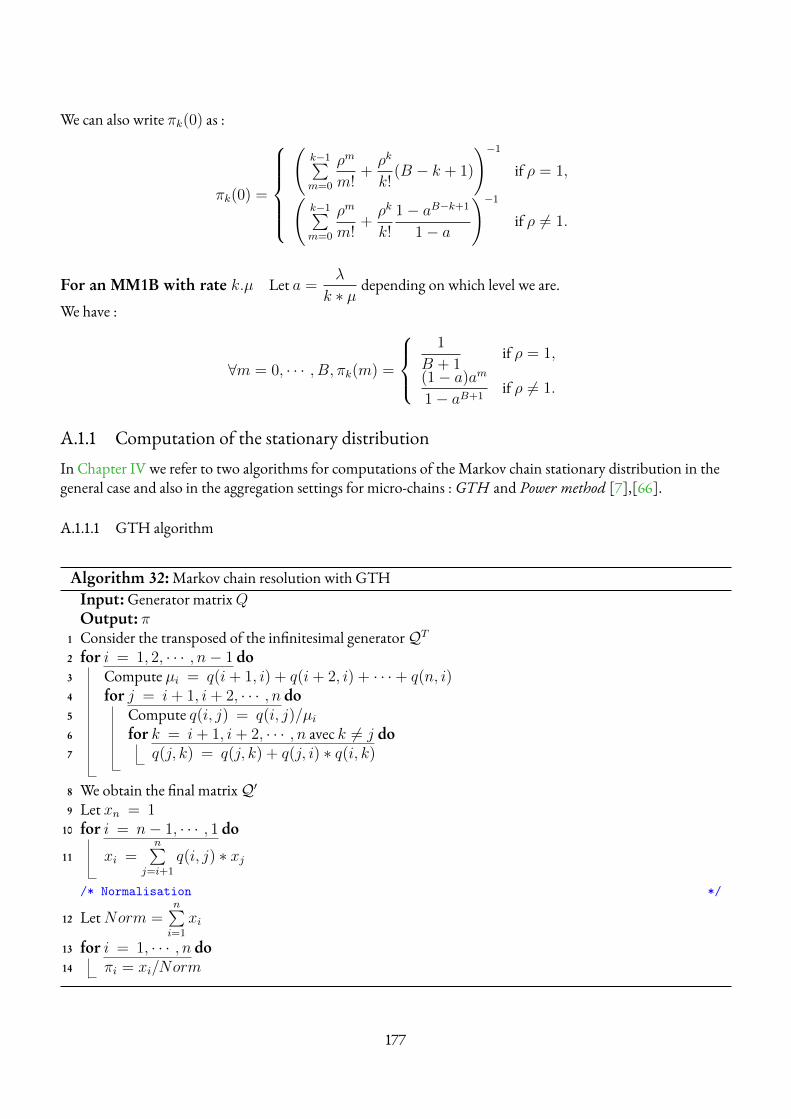
We can also write πk(0) as :

πk(0) =

(k−1∑m=0

ρm

m!+ρk

k!(B − k + 1)

)−1

if ρ = 1,(k−1∑m=0

ρm

m!+ρk

k!

1− aB−k+1

1− a

)−1

if ρ 6= 1.

For an MM1B with rate k.µ Let a =λ

k ∗ µdepending on which level we are.

We have :

∀m = 0, · · · , B, πk(m) =

1

B + 1if ρ = 1,

(1− a)am

1− aB+1if ρ 6= 1.

A.1.1 Computation of the stationary distributionIn Chapter IV we refer to two algorithms for computations of the Markov chain stationary distribution in thegeneral case and also in the aggregation settings for micro-chains :GTH and Power method [7],[66].

A.1.1.1 GTH algorithm

Algorithm 32:Markov chain resolution with GTHInput:Generator matrixQOutput: π

1 Consider the transposed of the infinitesimal generatorQT2 for i = 1, 2, · · · , n− 1 do3 Compute µi = q(i+ 1, i) + q(i+ 2, i) + · · ·+ q(n, i)4 for j = i+ 1, i+ 2, · · · , n do5 Compute q(i, j) = q(i, j)/µi6 for k = i+ 1, i+ 2, · · · , n avec k 6= j do7 q(j, k) = q(j, k) + q(j, i) ∗ q(i, k)

8 We obtain the final matrixQ′9 Let xn = 1

10 for i = n− 1, · · · , 1 do

11 xi =n∑

j=i+1

q(i, j) ∗ xj

/* Normalisation */

12 LetNorm =n∑i=1

xi

13 for i = 1, · · · , n do14 πi = xi/Norm

177

A.1.1.2 Power method

The Power method algorithm requires to uniformise the continuous timeMarkov chain first to solve πP = P .

Algorithm 33:The power methodInput: Probability transition matrix P ,K periodical renormalisations, ε precisionOutput: π/* Begin */

1 x← any probability distribution2 n← 03 repeat4 n← n+ 15 y ← x× P6 dist← ||x− y||7 x← y8 if nmodK = 0 then9 x←Renormalise(x)

10 until dist < ε11 π ←Renormalise(x)12 return π

Algorithm 34:Renormalise(x) : Renormalisation of a vectorInput:A vector of numbers x indexed by ]xOutput:A vector proportional to xwhich entries sum up to 1

1 Let S ← 02 for i ∈ ]x do3 S ← S + x[i]

4 for i ∈ ]x do5 x[i]← x[i]/S

6 return x

178

RESUME

11 rue SillyBoulogne-Billancourt 92100Francetournaire.thomas@hotmail.fr

FrenchJuly 17th, 1993+6 35 34 72 57thomas.tournaire@nokia.com

Research interest and skills— Reinforcement learning (RL) methods : performance enhancements with structured model-based

approaches (factored, causal, hierarchical)— RL-based solutions for complex network optimization (Multi-Queuing systems and 5G use-cases)— Programming skills : Python (Keras, Tensorflow, Numpy, Pandas, Scipy, Simpy), MatLab-Simulink, C++

Work Experience

2019-2022 Research Engineer at Nokia Bell Labs France, NozayAI research, Maths&Algorithms Root Cause Analysis

2021-2021 Contract Teacher at University Nanterre Paris XMachine Learning, Neural Networks and Deep RL course, M2 D3S-IESPython-VBA course, M2 ISEFAR

2018-2019 Research Intern at Telecom SudParis, EvryStochastic optimisation of performances and energy consumption in the cloud, PGMO-BOBIBEEStochastic optimisation problem addressed using combinatorial optimisation methods,Markov Chain, performance evaluation and stochastic dynamic programming methods

179

Education

2019–2022 PhD in Computer Science, IP Paris, Telecom sudParisTitle : Reducing energy consumption in largescale networks withMDP and RLSupervisors : Hind Castel-Taleb, Emmanuel Hyon, Armen Aghasaryan

2017–2018 Master 2Mathematical Modelling andMethods in Economy and FinanceOptimisation and Operational Research track, mention BienUniversity Paris 1, Panthéon-Sorbonne, France

2016-2017 Master 1 International Master in Mathematics applied to Economics and Finance, men-tion Bien, 1stMasterThesis :MeasureTheory, Extension ofMeasures byKolmogorov andLebesgue andmathematical ExpectationAdvisor : Bernard DeMeyer

2013-2016 Bachelor Mathematics and Informatics applied to human and social sciences, mentionTrès Bien, 1stUniversity Versailles Saint-Quentin en Yvelines

2011-2012 Baccalauréat série S, Spécialité Mathématiques, Mention Très BienLycée La Bruyère, Versailles

Prizes∗ Winner of the Nokia French Student Award, Bell Labs Section, July 2020

Publications

In preparation— Optimal control policies for resource allocation in the Cloud : comparison betweenMarkov decision

process and heuristic approaches, T. Tournaire, H. Castel-Taleb, E. Hyon, submitted to the journalSimulation Modelling Practice and Theory and available at arXiv preprint arXiv :2104.14879

International conferences with proceedings and referees[1] Factored reinforcement learning for auto-scaling in tandem queues, IEEE NOMS, Apr. 2022, T.

Tournaire, Y. Jin, A. Aghasaryan, H. Castel-Taleb, E. Hyon[2] Reinforcement learning with model-based approaches for dynamic resource allocation in a tandem queue,

26th International Conference on Analytical & Stochastic Modelling Techniques & Applications, Aug.2021, T. Tournaire, J. Barthélémy, H. Castel-Taleb, E. Hyon

[3] Generating optimal thresholds in a hysteresis queue : application to a cloud model, IEEE Mascots, p.283-294, Oct. 2019, T. Tournaire, H. Castel-Taleb, E. Hyon, T. Hoche (24% selection rate)

National conferences with proceedings and referees[1] Génération de seuils optimaux dans une file hystérésis, CORES, Jun. 2019, T. Tournaire, H. Castel-Taleb,

E. Hyon, T. Hoche (50% selection rate)

180

National conferences with abstract selection∗ Factored model-based RL for tandem queues resource allocation, PGMO, Dec. 2021, T. Tournaire, Y. Jin,A. Aghasaryan∗ Comparaisons de méthodes de calcul de seuils pour minimiser la consommation énergétique d’un cloud,ROADEF, Nov. 2019, T. Tournaire, H. Castel-Taleb, E. Hyon∗ Stochastic optimisation of energy consumption and performance in a cloud system, PGMO, Dec. 2018, T.Tournaire, H. Castel-Taleb, E. Hyon

Patents[P1] AI/ML based PDCP Split in Dual/Multi Connectivity Configurations : Collective Inference/Decision

and Impact on 3gpp Interfaces, F. SyedMuhammad, R. Damodaran, T. Tournaire, A. Feki, L. Maggi, F.Durand, U. Chowta (submittedMarch 29, 2021)

[P2] Multi-Agent Reinforcement Learning Sharing CommonNeural Network Policy for PDCPData Split, T.Tournaire, F. SyedMuhammad, A. Feki, L. Maggi, F. Durand (filed November 11, 2021)

Diverse presentations∗ Causal RL,Nokia Bell Labs Show & Tell, Mar. 2021∗ Causal RL,Nokia France PhD Seminar, Mar. 2021∗ SimPy package tutorial, LINCS, Nov. 2020∗ Model-Based RL, RL Reading Group in Hyper Industrial Analytics Group at Nokia Bell Labs, Mar. 2020∗ Performance and Cost Optimisation in the future 5G Cloud, Poster,Doctorant Day TSP, Dec. 2019

Teaching∗ VBA/Python TD,M2 ISEFAR, University Paris Nanterre, 2020 (12h), 2021 (22h)∗ ML, Neural Networks, Deep RL course, M2 D3S-IES, 2021 (8h)

Intern supervision∗ François Pic : Hierarchical MDP for tandem queue, with H. Castel and E. Hyon, 2021∗ Jeanne Barthélémy : Model-based RL for tandem queue, with H. Castel and E. Hyon, 2020

Trainings∗ Ethics in Scientific Research, February 2022, IP Paris∗ Reinforcement Learning virtual school, ANITI, Mar. 2021∗ Cosmos : Optimisation and Reinforcement Learning, Nov. 2019, INRIA, Paris∗ ResCom summer school : models and methods of network analysis, June 2019, Anglet

181

∗ Data Science Working Group— Frommachine learning basics to Feed Forward Neural Networks, 2019, Telecom SudParis— Optimisation for machine/deep learning, 2019, Telecom SudParis— Queuing theory seminar : A. Brandwajn Talk, 2019, Telecom SudParis

∗ Student Volunteer at IEEE Infocom, May 2019, Paris∗ AI ENS workshop : Machine Learning and User DecisionMaking, May 2019, Paris∗ Nokia Bell Labs Trainings : AmazonWeb Services day, Oct. 2019 andWorld Class Presentation, Dec. 2019,Nozay

Languages

French Mother tongueEnglish Fluent

182

RÉSUMÉ EN FRANÇAIS ÉLARGI

IntroductionL’émergence de nouvelles technologies (villes intelligentes, milieu hospitalier, véhicules autonomes, IoT, etc.)nécessite une allocation efficace des ressources pour satisfaire la demande. Cependant, ces nouveaux besoinsnécessitent une puissance de calcul élevée impliquant une plus grande consommation d’énergie notammentdans les infrastructures cloud et data centers. Il est donc essentiel de trouver de nouvelles solutions qui peuventsatisfaire ces besoins tout en réduisant la consommation d’énergie des ressources. Dans cette thèse, nousproposons et comparons de nouvelles solutions d’IA (apprentissage par renforcement RL) pour orchestrer lesressources virtuelles dans les environnements de réseaux virtuels de manière à garantir les performances etminimiser les coûts opérationnels. Nous considérons les systèmes de file d’attente comme un modèle pour lesinfrastructures cloud IaaS (Infrastructure as a Service) et apportons des méthodes d’apprentissage pour allouerefficacement le bon nombre de ressources. Notre objectif est de minimiser une fonction de coût en tenantcompte des coûts de performance et opérationnels/énergétiques. Nous utilisons différents types d’algorithmesde RL (du « sans-modèle » au «modèle relationnel ») pour apprendre la meilleure politique. L’apprentissagepar renforcement s’intéresse à la manière dont un agent doit agir dans un environnement pour maximiser unerécompense cumulative. Nous développons d’abord un modèle de files d’attente d’un système cloud avec unnœud physique hébergeant plusieurs ressources virtuelles. Dans cette première partie, nous supposons quel’agent connaît le modèle (dynamiques de l’environnement et coût), ce qui lui donne la possibilité d’utiliser desméthodes de programmation dynamique pour le calcul de la politique optimale. Puisque le modèle est connudans cette partie, nous nous concentrons également sur les propriétés des politiques optimales, qui sont desrègles basées sur les seuils et l’hystérésis. Cela nous permet d’intégrer la propriété structurelle des politiques dansles algorithmes MDP. Après avoir fourni un modèle de cloud concret avec des arrivées exponentielles avec desintensités réelles et des données d’énergie pour le fournisseur de cloud, nous comparons dans cette premièreapproche l’efficacité et le temps de calcul des algorithmes MDP par rapport aux heuristiques construites sur lesdistributions stationnaires de la chaîne de Markov des files d’attente.L’objectif affiché de la thèse est double. Il s’agit d’une part d’apprendre la politique optimale d’allocation deressources dans un environnement de type cloud et d’autre part de concevoir des méthodes d’apprentissages quisoient à la fois efficientes et adaptées aux problématiques auxquelles est confronté le monde industriel. Lescontributions de la thèse sont réparties en plusieurs chapitres, résumées ci-dessous.

183

LittératureCe chapitre présente une revue de la littérature sur le Cloud computing, la gestion de l’énergie, les modèles de filed’attente et les techniques d’optimisation pour l’allocation de ressources dans les systèmes à grande échelles(centres de calcul, centres de stockages, etc.). Il présente tout d’abord ce qu’est le Cloud, comment il se comporte,les infrastructures et modèles existants (par exemple, les centres de données) et le cadre de la virtualisation.Ensuite, il donne un aperçu du domaine de la gestion de l’énergie en présentant le besoin, les solutions pourmesurer et modéliser l’énergie dans le Cloud ainsi que le paradigme d’allocation dynamique des ressources.Enfin, il présente les politiques d’auto-dimensionnement dans le Cloud existantes avec des règles basées sur desseuils, des modèles de file d’attente et des techniques de gestion du contrôle et d’apprentissage par renforcement.Pour optimiser la consommation énergétique des systèmes considérés, la méthode retenue dans ce document estla mise en veille des ressources inutilisées. Il s’agit donc d’activer et de désactiver des noeuds de calcul au cours dutemps selon la demande et les engagements pris sur le niveau de service.

Apprentissage par renforcementLe chapitre 3 présente plus en détail les méthodes d’apprentissage qui seront considérées et étudiées dans leschapitres suivants. On introduit les bases des processus de décisionMarkoviens avec leurs différentes méthodesde résolution et les bases de l’apprentissage par renforcement. Les méthodes sont présentées selon le degré deconnaissance du contrôleur, allant de la connaissance parfaite du modèle du système (dynamique et coût) àl’absence de modèle. La présentation ici préfigure l’ordre de présentation des contributions dans les chapitressuivants. Ce chapitre fournit également un bref résumé de deux cas d’applications industrielles de l’apprentissagerenforcé sans modèle. Le retour d’expérience apparait mitigé puisque les méthodes utilisées se sont révéléesintéressantes et compétitives dans un cas sur les deux. Le chapitre se conclut sur une comparaison des avantageset des inconvénients des méthodes avec ou sans modèle.

Processus de décisionMarkovien ouHeuristiques : Comment calculer les poli-tiques d’auto-dimensionnement dans un système de files d’attente avec unmo-dèle connuDans ce chapitre, nous considérons que l’agent reçoit le véritable modèle de l’environnementM et nous situonsdonc dans la classe des algorithmes d’apprentissage par renforcement avec modèle, où le modèle estpréalablement connu par l’agent. Nous considérons un problème d’optimisation d’un coût global tenantcompte de différents coûts : associés aux exigences de performance définies dans un accord de niveau de service(SLA) et des coûts représentant la consommation d’énergie. Nous voulons calculer la politique optimaled’activation et de désactivation des serveurs en fonction de l’occupation des requêtes dans la file d’attente. Dansce chapitre, nous étudions des modèles dans lesquels la structure de la politique est de type hystérésis.Cependant, supposer que la politique a une forme d’hystérésis n’est pas suffisant pour caractérisercomplètement la politique optimale. Il faut déterminer les valeurs concrètes des seuils. A cette fin, il existe deuxapproches de modélisation qui correspondent à deux courants majeurs de la littérature. La première exprime leproblème dans un modèle de problème d’optimisation déterministe. Elle est réalisée par l’utilisation de la valeurmoyenne des coûts calculée par la distribution stationnaire d’une CTMC (Continuous TimeMarkov Chains).La seconde exprime le problème sous un modèle MDP avec des politiques structurées et calcule la politiqueoptimale. Mais, bien qu’elles soient les plus utilisées pour le calcul des seuils, l’efficacité de ces deux approches

184

n’est pas évaluée très soigneusement pour le calcul des seuils uniques par niveau. En particulier, cela n’a jamaisété fait pour les politiques d’hystérésis. Peu de travaux se sont concentrés sur l’optimalité de la politiqued’hystérésis pour les modèles de Cloud mais, à notre connaissance, aucun sur le calcul des seuils. Déterminerquelle est la meilleure approche prometteuse et quel est le meilleur modèle à choisir dans une utilisationpratique est donc un point important qui est abordé ici.Nous validons également notre approche avec un modèle réel. L’approche est difficile car, à notre connaissance,il n’existe pas, dans la littérature, un modèle unifié incluant à la fois l’énergie, la qualité de de service et lesparamètres du trafic réel. Nous proposons de construire un coût global prenant en compte à la fois laconsommation réelle d’énergie, les coûts financiers réels des machines virtuelles et de l’accord de niveau deservice (SLA) simultanément. Nous proposons de construire un coût global prenant en compte à la fois laconsommation d’énergie réelle, les coûts financiers réels des machines virtuelles et les accords de niveau deservice (SLA). Nous pensons que le modèle présenté est suffisamment générique pour représenter une largeclasse de problèmes et est suffisant pour donner une une signification pertinente à tous les paramètres. Grâce ànos algorithmes et à ce modèle, les gérants de Cloud peuvent générer des coûts optimisés significatifs dans des casréels.Toutefois, ce chapitre émet une hypothèse très forte : assummer que l’agent connait le modèle exact del’environnement. En pratique, c’est rarement le cas et il faut trouver des solutions plus adaptées qui peuventapprendre une politique optimale dans des environnements partiellement connus.

Apprentissage par renforcement basé sur un modèle pour les réseaux multi-tiersUn des défi majeur de l’allocation des ressources dans le Cloud porte sur le fait que les experts ne connaissent pasfacilement les statistiques exactes du système (arrivées des requêtes, taux de services) dans les environnementsréels, car ils évoluent trop rapidement. Par conséquent, un agent logiciel ne possède aucun modèle précis del’environnement pour le calcul de la politique optimale. Cela nécessite l’implémentation de solutionsd’apprentissage par renforcement qui permettent l’apprentissage de politiques dans des environnementsinconnus. D’autre part, nous ne sommes pas sûrs que les approches des praticiens soient robustes (souvent trèsexpérimentales). La plupart des travaux concernant l’apprentissage par renforcement pour l’allocation deressources dans le Cloud sont consacrés à des techniques sans modèle telles que l’algorithme du Q-Learning ouou de l’apprentissage par renforcement profond, mais il n’existe aucune application de techniques basées sur desmodèles pour de tels problématiques.Dans ce chapitre, nous voulons évaluer les approches d’apprentissage par renforcement basées sur les modèlesdans le cas des réseaux de files d’attente, ce qui a été peu fait jusqu’à présent. De plus, nous voulons étendre lagamme des modèles étudiés dans le chapitre précédent pour aller au-delà du simple modèle multi-serveur enconsidérant une application réseau avec plusieurs files d’attente, ce qui permet de mieux représenter lesarchitectures multi-tiers, ce qui n’a pas non plus été beaucoup fait dans la littérature. Par conséquent, noussupposons maintenant que l’agent logiciel ne porte pas la connaissance du modèle MDP. L’objectif est doncd’adopter les approches RL basées sur les modèles, en particulier les architectures Dyna et les techniques decontrole adaptatif afin d’évaluer leur pertinence, si jamais, ou de les améliorer pour l’allocation dynamique desressources dans les systèmes de réseaux de files d’attente. De plus, nous voulons évaluer la robustesse de cesapproches dans des cas d’utilisation où les arrivées peuvent arriver massivement de manière très brusque.Ce chapitre donne d’abord un aperçu plus détaillé des techniques d’apprentissage par renforcement basées surdes modèles, puis présente deux modèles de file d’attente pour exprimer les architectures de réseau multi-tiers. Ilmontre ensuite comment nous avons sélectionné les techniques d’apprentissage par renforcement basées sur des

185

modèles en fournissant un algorithme général et comment nous les avons paramétrées pour les comparer à l’étatde l’art de l’apprentissage par renforcement sans modèle sur un réseau Cloud multi-tier. Enfin, nous présentonsles résultats de la comparaison entre les techniques RL sur différents scénarios et paramètres de Cloud dans unenvironnement simulé, démontrant le gain des techniques RL basées sur le modèle.

Apprentissage par renforcement factorisé pour les réseaux multi-tiersDans les chapitres précédents, nous n’avons considéré que des représentations tabulaires de la dynamique et desmodèles de récompense, ce qui peut s’avérer peu pratique dans des environnements à grande échelle avec desespaces d’état et d’action de très grande taille. Le cadre de l’apprentissage par renforcement factorisé permet dereprésenter de manière plus compacte le modèleM de l’environnement en intégrant les relations entre lesvariables d’environnement. Dans les environnements qui ont des relations spécifiques entre les variables d’état, ilpourrait être très bénéfique d’utiliser cette représentation pour accélérer la convergence et la facilitéd’implémentation.La dernière partie, divisé en deux chapitres, se concentre donc sur les techniques de RL basées sur des modèlesavec une structure relationnelle entre les variables d’état. Comme ces réseaux en tandem ont des propriétésstructurelles dues à la forme de l’infrastructure Cloud, nous intégrons les approches factorisées et causales auxméthodes de RL pour inclure cette connaissance. Nous fournissons à l’agent une connaissance relationnelle del’environnement qui lui permet de comprendre comment les variables sont reliées. L’objectif principal estd’accélérer la convergence : d’abord avec une représentation plus compacte avec la factorisation où nousconcevons un algorithme en ligne de MDP factorisé que nous comparons avec des algorithmes de RL sansmodèle et basés sur un modèle ; ensuite en intégrant le raisonnement causal et contrefactuel qui peut traiter lesenvironnements avec des observations partielles et des facteurs de confusion non observés.

ConclusionLe chapitre 8 présente une nouvelle taxonomie de toutes les méthodes d’apprentissage abordées et mentionnéesdans la thèse, avec une vision structurelle de l’apprentissage par renforcement découplé en 3 socles : MDP, MDPfactorisé et MDP causal. Finalement, le chapitre reprend toutes les contributions et leurs perspectives, etnotamment les différentes pistes envisagées afin de consolider la partie expérimentale.

186

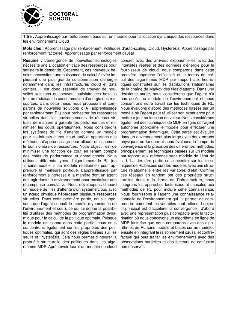
Titre : Apprentissage par renforcement base sur un modele pour l’allocation dynamique des ressources dansles environnements Cloud

Mots cles : Apprentissage par renforcement, Politiques d’auto-scaling, Cloud, Hysteresis, Apprentissage parrenforcement factorise, Apprentissage par renforcement causal

Resume : L’emergence de nouvelles technologiesnecessite une allocation efficace des ressources poursatisfaire la demande. Cependant, ces nouveaux be-soins necessitent une puissance de calcul elevee im-pliquant une plus grande consommation d’energienotamment dans les infrastructures cloud et datacenters. Il est donc essentiel de trouver de nou-velles solutions qui peuvent satisfaire ces besoinstout en reduisant la consommation d’energie des res-sources. Dans cette these, nous proposons et com-parons de nouvelles solutions d’IA (apprentissagepar renforcement RL) pour orchestrer les ressourcesvirtuelles dans les environnements de reseaux vir-tuels de maniere a garantir les performances et mi-nimiser les couts operationnels. Nous consideronsles systemes de file d’attente comme un modelepour les infrastructures cloud IaaS et apportons desmethodes d’apprentissage pour allouer efficacementle bon nombre de ressources. Notre objectif est deminimiser une fonction de cout en tenant comptedes couts de performance et operationnels. Nousutilisons differents types d’algorithmes de RL (du� sans-modele � au modele relationnel) pour ap-prendre la meilleure politique. L’apprentissage parrenforcement s’interesse a la maniere dont un agentdoit agir dans un environnement pour maximiser unerecompense cumulative. Nous developpons d’abordun modele de files d’attente d’un systeme cloud avecun nœud physique hebergeant plusieurs ressourcesvirtuelles. Dans cette premiere partie, nous suppo-sons que l’agent connaıt le modele (dynamiques del’environnement et cout), ce qui lui donne la possibi-lite d’utiliser des methodes de programmation dyna-mique pour le calcul de la politique optimale. Puisquele modele est connu dans cette partie, nous nousconcentrons egalement sur les proprietes des poli-tiques optimales, qui sont des regles basees sur lesseuils et l’hysteresis. Cela nous permet d’integrer lapropriete structurelle des politiques dans les algo-rithmes MDP. Apres avoir fourni un modele de cloud

concret avec des arrivees exponentielles avec desintensites reelles et des donnees d’energie pour lefournisseur de cloud, nous comparons dans cettepremiere approche l’efficacite et le temps de cal-cul des algorithmes MDP par rapport aux heuris-tiques construites sur les distributions stationnairesde la chaıne de Markov des files d’attente. Dans unedeuxieme partie, nous considerons que l’agent n’apas acces au modele de l’environnement et nousconcentrons notre travail sur les techniques de RL.Nous evaluons d’abord des methodes basees sur unmodele ou l’agent peut reutiliser son experience pourmettre a jour sa fonction de valeur. Nous consideronsegalement des techniques de MDP en ligne ou l’agentautonome approxime le modele pour effectuer uneprogrammation dynamique. Cette partie est evalueedans un environnement plus large avec deux nœudsphysiques en tandem et nous evaluons le temps deconvergence et la precision des differentes methodes,principalement les techniques basees sur un modelepar rapport aux methodes sans modele de l’etat del’art. La derniere partie se concentre sur les tech-niques de RL basees sur des modeles avec une struc-ture relationnelle entre les variables d’etat. Commeces reseaux en tandem ont des proprietes struc-turelles dues a la forme de l’infrastructure, nousintegrons les approches factorisees et causales auxmethodes de RL pour inclure cette connaissance.Nous fournissons a l’agent une connaissance rela-tionnelle de l’environnement qui lui permet de com-prendre comment les variables sont reliees. L’objec-tif principal est d’accelerer la convergence : d’abordavec une representation plus compacte avec la facto-risation ou nous concevons un algorithme en ligne deMDP factorise que nous comparons avec des algo-rithmes de RL sans modele et bases sur un modele ;ensuite en integrant le raisonnement causal et contre-factuel qui peut traiter les environnements avec desobservations partielles et des facteurs de confusionnon observes.

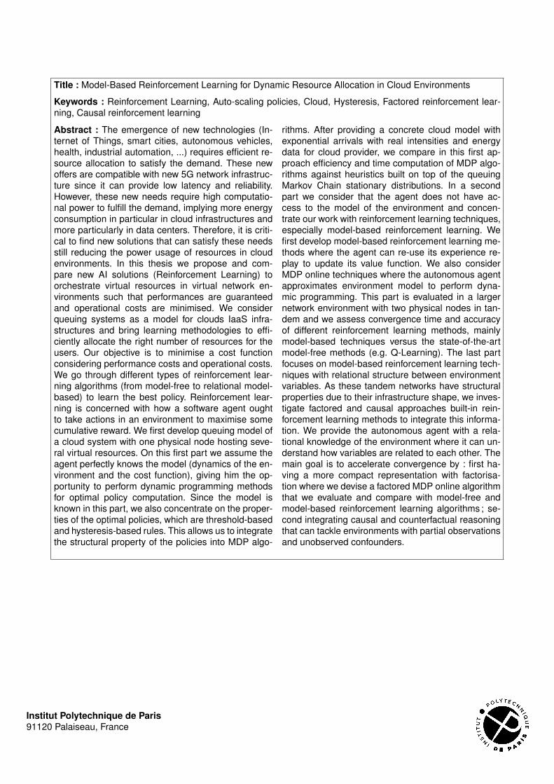
Title : Model-Based Reinforcement Learning for Dynamic Resource Allocation in Cloud Environments

Keywords : Reinforcement Learning, Auto-scaling policies, Cloud, Hysteresis, Factored reinforcement lear-ning, Causal reinforcement learning

Abstract : The emergence of new technologies (In-ternet of Things, smart cities, autonomous vehicles,health, industrial automation, ...) requires efficient re-source allocation to satisfy the demand. These newoffers are compatible with new 5G network infrastruc-ture since it can provide low latency and reliability.However, these new needs require high computatio-nal power to fulfill the demand, implying more energyconsumption in particular in cloud infrastructures andmore particularly in data centers. Therefore, it is criti-cal to find new solutions that can satisfy these needsstill reducing the power usage of resources in cloudenvironments. In this thesis we propose and com-pare new AI solutions (Reinforcement Learning) toorchestrate virtual resources in virtual network en-vironments such that performances are guaranteedand operational costs are minimised. We considerqueuing systems as a model for clouds IaaS infra-structures and bring learning methodologies to effi-ciently allocate the right number of resources for theusers. Our objective is to minimise a cost functionconsidering performance costs and operational costs.We go through different types of reinforcement lear-ning algorithms (from model-free to relational model-based) to learn the best policy. Reinforcement lear-ning is concerned with how a software agent oughtto take actions in an environment to maximise somecumulative reward. We first develop queuing model ofa cloud system with one physical node hosting seve-ral virtual resources. On this first part we assume theagent perfectly knows the model (dynamics of the en-vironment and the cost function), giving him the op-portunity to perform dynamic programming methodsfor optimal policy computation. Since the model isknown in this part, we also concentrate on the proper-ties of the optimal policies, which are threshold-basedand hysteresis-based rules. This allows us to integratethe structural property of the policies into MDP algo-

rithms. After providing a concrete cloud model withexponential arrivals with real intensities and energydata for cloud provider, we compare in this first ap-proach efficiency and time computation of MDP algo-rithms against heuristics built on top of the queuingMarkov Chain stationary distributions. In a secondpart we consider that the agent does not have ac-cess to the model of the environment and concen-trate our work with reinforcement learning techniques,especially model-based reinforcement learning. Wefirst develop model-based reinforcement learning me-thods where the agent can re-use its experience re-play to update its value function. We also considerMDP online techniques where the autonomous agentapproximates environment model to perform dyna-mic programming. This part is evaluated in a largernetwork environment with two physical nodes in tan-dem and we assess convergence time and accuracyof different reinforcement learning methods, mainlymodel-based techniques versus the state-of-the-artmodel-free methods (e.g. Q-Learning). The last partfocuses on model-based reinforcement learning tech-niques with relational structure between environmentvariables. As these tandem networks have structuralproperties due to their infrastructure shape, we inves-tigate factored and causal approaches built-in rein-forcement learning methods to integrate this informa-tion. We provide the autonomous agent with a rela-tional knowledge of the environment where it can un-derstand how variables are related to each other. Themain goal is to accelerate convergence by : first ha-ving a more compact representation with factorisa-tion where we devise a factored MDP online algorithmthat we evaluate and compare with model-free andmodel-based reinforcement learning algorithms ; se-cond integrating causal and counterfactual reasoningthat can tackle environments with partial observationsand unobserved confounders.

Institut Polytechnique de Paris91120 Palaiseau, France