a reinforcement learning -adaptive control architecture for morphing

JOURNAL OF AEROSPACE COMPUTING, INFORMATION, AND COMMUNICATIONVol. 2, April 2005

A Reinforcement Learning - Adaptive ControlArchitecture for Morphing

John Valasek,∗ Monish D. Tandale,† and Jie Rong‡

Texas A&M University, College Station, Texas 77843-3141

This paper develops a control methodology for morphing, which combines Machine Learn-ing and Adaptive Dynamic Inversion Control. The morphing control function, which usesReinforcement Learning, is integrated with the trajectory tracking function, which usesStructured Adaptive Model Inversion Control. Optimality is addressed by cost functions rep-resenting optimal shapes corresponding to specified operating conditions, and an episodicReinforcement Learning simulation is developed to learn the optimal shape change policy.The methodology is demonstrated by a numerical example of a 3-D morphing air vehicle,which simultaneously tracks a specified trajectory and autonomously morphs over a set ofshapes corresponding to flight conditions along the trajectory. Results presented in the papershow that this methodology is capable of learning the required shape and morphing into it,and accurately tracking the reference trajectory in the presence of parametric uncertaintiesand initial error conditions.

Nomenclatureα learning rateβ positive step-size parameterδ temporal difference errorε tracking error for linear statesε tracking error for angular statesγ discount factorπ reinforcement learning policy�j(s) basis functionρ density of airσ = [φ θ ψ]T 3-2-1 Euler angles that describe the orientation of the body axes relative to the inertial

axesσ r Euler angles for the reference trajectoryθpa parameter vector for approximating the preference functionθv parameter vector for approximating the value function� true inertia parameter vector� adaptive inertia parameter vector

Received 18 March 2001; revision received 30 July 2003; accepted for publication 26 August 2003. Copyright © 2005 bythe American Institute of Aeronautics and Astronautics, Inc. All rights reserved. Copies of this paper may be made for personalor internal use, on condition that the copier pay the $10.00 per-copy fee to the Copyright Clearance Center, Inc., 222 RosewoodDrive, Danvers, MA 01923; include the code 1542-9423/04 $10.00 in correspondence with the CCC.∗Associate Professor & Director, Flight Simulation Laboratory, Aerospace Engineering Department. Associate Fellow, [email protected], http://jungfrau.tamu.edu/valasek/† Graduate Research Assistant, Flight Simulation Laboratory, Aerospace Engineering Department. Student Member, [email protected]‡ Graduate Research Assistant, Flight Simulation Laboratory, Aerospace Engineering Department. Student Member, [email protected]

174

http://jungfrau.tamu.edu/valasek/

mailto: [email protected]

mailto: [email protected]

VALASEK, TANDALE, AND RONG

� error between adaptive and true inertia parameter vectorτ 6× 6 symmetric positive definite matrix� positive scalar constantω = [p q r]T angular velocity of the smart block along the body axesω matrix representation of the cross product between ω and a compatible vectorA(st ) set of actions available in state stcj preselected center states vectorCφ cos(φ)Cda,Kda design matricesCy,Cz center state vectorsf flight conditionF control forceFd drag forceH basis vector for function approximationI mass moments of inertia of the smart block in the body axesJl nonlinear transformation relating pc and vcJa nonlinear transformation relating σ and ω

J cost functionJy cost function component corresponding to the y dimensionJz cost function component corresponding to the z dimensionm mass of the smart blockm adaptive parameter that learns the massM control momentMd drag momentpc = [X Y Z]T position of the center of mass of the smart block along the inertial axesp(s, a) preference function: tendency to select action a at state sR rewardR weighting matrixS set of possible states for reinforcement learningSθ sin(θ)Sy(f ) optimal y dimension at flight condition fSz(f ) optimal z dimension at flight condition fvc = [u v w]T linear velocity of the smart block along the body axesV Lyapunov functionV π(s) state value function for policy πVy voltage control for the y dimensionVz voltage control for the z dimension[XbYbZb]T body axes[XNYNZN ]T inertial axes[x y z]T dimension of the smart block along the body axesYa(σ , σ , σ ) regression matrix

I. Introduction

CURRENT interest in morphing vehicles has been fuelled by advances in smart technologies, including mate-rials, sensors, actuators, and their associated support hardware and microelectronics. Morphing research has

led to a series of breakthroughs in a wide variety of disciplines that, when fully realized for aircraft applica-tions, have the potential to produce large increments in aircraft system safety, affordability, and environmentalcompatibility.1 Although there are several definitions and interpretations of the term morphing, it is generally agreedthat the concept refers to large scale shape changes or transfigurations. Various organizations which are researching

175


morphing technologies for both air and space vehicles have adopted their own definitions according to their needs.The National Aeronautics and Space Administration’s (NASA) Morphing Project defines morphing as an efficient,multi-point adaptability that includes macro, micro, structural and/or fluidic approaches. 2 The Defense AdvancedResearch Projects Agency (DARPA) uses the definition of a platform that is able to change its state substantially(on the order of 50%) to adapt to changing mission environments, thereby providing a superior system capabilitythat is not possible without reconfiguration. Such a design integrates innovative combinations of advanced materials,actuators, flow controllers, and mechanisms to achieve the state change.3

In spite of their relevance, these definitions do not adequately address or describe the supervisory and controlaspects of morphing. Reference 4 attempts to do so by making a distinction between Morphing for MissionAdaptation,and Morphing for Control. In the context of flight vehicles, Morphing for MissionAdaptation is a large scale, relativelyslow, in-flight shape change to enable a single vehicle to perform multiple diverse mission profiles. Conversely,Morphing for Control is an in-flight physical or virtual shape change to achieve multiple control objectives, such asmaneuvering, flutter suppression, load alleviation and active separation control. In this paper, the authors considerthe problem of Morphing for Mission Adaptation.

In the context of intelligent systems, three essential functionalities of a practical Morphing for Mission Adaptationcapability are:

1. When to reconfigure2. How to reconfigure3. Learning to reconfigureWhen to reconfigure is driven by mission priorities/tasks, and leads to optimal shape being a system parameter.

In the context of a reconfigurable vehicle such as an aircraft, each shape results in performance values (speed,range, endurance, etc.) at specific flight conditions (Mach number, altitude, angle-of-attack, and sideslip angle).It is a major issue, as the inability for a given aircraft to perform multiple missions successfully can directly beattributed to shape, at least if aerodynamic performance is the primary consideration. This is because for a given taskor mission, there is usually an ideal or optimal vehicle shape, e.g. configuration.4 However, this optimality criteriamay not be known over the entire flight envelope in actual practice, and the mission may be modified or completelychanged during operation. How to reconfigure is a problem of sensing, actuation, and control. 5 They are importantand challenging since large shape changes produce time-varying vehicle properties, and especially, time-varyingmoments and products of inertia. The controller must therefore be sufficiently robust to handle these potentiallywide variations. Learning to reconfigure is perhaps the most challenging of the three functionalities, and the onewhich has received the least attention. Even if optimal shapes are known, the actuation scheme(s) to produce themmay be only poorly understood, or not understood at all; Reinforcement Learning is therefore a candidate approach.It is important that learning how to reconfigure is also life-long learning. This will enable the vehicle to be moresurvivable, operate more safely, and be multi-role.

This paper proposes and develops a conceptual control architecture which addresses these essential functionalitiesof Morphing for Mission Adaptation. Called Adaptive-Reinforcement Learning Control (A-RLC), it is a marriage ofAdaptive Dynamic Inversion Control and Machine Learning. By comparison to morphing research reported in theliterature which focus on structures and actuation, A-RLC addresses the optimal shape changing of an entire vehicle.A-RLC learns the commands which produce the optimal shape, defined as a function of operating condition, whilemaintaining accurate trajectory tracking. A-RLC uses Structured Adaptive Model Inversion (SAMI) as the trajectorytracking controller for handling time-varying properties, parametric uncertainties, and disturbances. For learningthe optimality relations between the operating conditions and the shape, and learning how to produce the optimalshape at every operating condition over the life of the vehicle, A-RLC uses Reinforcement Learning. Optimality isaddressed with cost functions which penalize deviations from the optimal shape. The paper first defines the shapechanging dynamics of a hypothetical three-dimensional Smart Block air vehicle of constant volume, which can morphin all the three spatial dimensions. The Reinforcement Learning module of A-RLC is developed next, and uses anactor-critic method to learn how to morph into specified shapes. This is followed by development of the SAMIcontrol module, which handles Smart Block parametric uncertainties, and initial error conditions, while trackinga trajectory. The A-RLC methodology is demonstrated with a numerical example of the Smart Block air vehicleautonomously morphing over a set of optimal shapes, corresponding to specified flight conditions, while tracking aspecified trajectory.

176


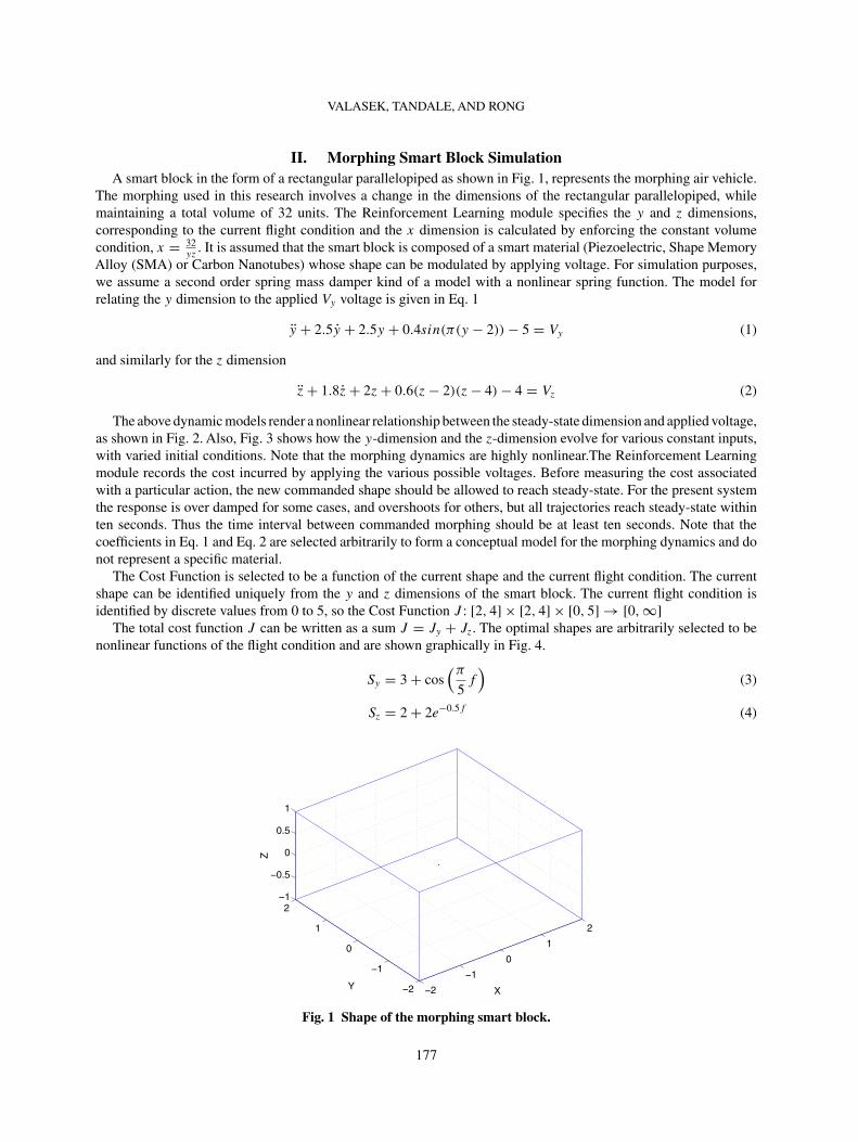
II. Morphing Smart Block SimulationA smart block in the form of a rectangular parallelopiped as shown in Fig. 1, represents the morphing air vehicle.

The morphing used in this research involves a change in the dimensions of the rectangular parallelopiped, whilemaintaining a total volume of 32 units. The Reinforcement Learning module specifies the y and z dimensions,corresponding to the current flight condition and the x dimension is calculated by enforcing the constant volumecondition, x = 32

yz. It is assumed that the smart block is composed of a smart material (Piezoelectric, Shape Memory

Alloy (SMA) or Carbon Nanotubes) whose shape can be modulated by applying voltage. For simulation purposes,we assume a second order spring mass damper kind of a model with a nonlinear spring function. The model forrelating the y dimension to the applied Vy voltage is given in Eq. 1

y + 2.5y + 2.5y + 0.4sin(π(y − 2))− 5 = Vy (1)

and similarly for the z dimension

z+ 1.8z+ 2z+ 0.6(z− 2)(z− 4)− 4 = Vz (2)

The above dynamic models render a nonlinear relationship between the steady-state dimension and applied voltage,as shown in Fig. 2. Also, Fig. 3 shows how the y-dimension and the z-dimension evolve for various constant inputs,with varied initial conditions. Note that the morphing dynamics are highly nonlinear.The Reinforcement Learningmodule records the cost incurred by applying the various possible voltages. Before measuring the cost associatedwith a particular action, the new commanded shape should be allowed to reach steady-state. For the present systemthe response is over damped for some cases, and overshoots for others, but all trajectories reach steady-state withinten seconds. Thus the time interval between commanded morphing should be at least ten seconds. Note that thecoefficients in Eq. 1 and Eq. 2 are selected arbitrarily to form a conceptual model for the morphing dynamics and donot represent a specific material.

The Cost Function is selected to be a function of the current shape and the current flight condition. The currentshape can be identified uniquely from the y and z dimensions of the smart block. The current flight condition isidentified by discrete values from 0 to 5, so the Cost Function J : [2, 4] × [2, 4] × [0, 5] → [0,∞]

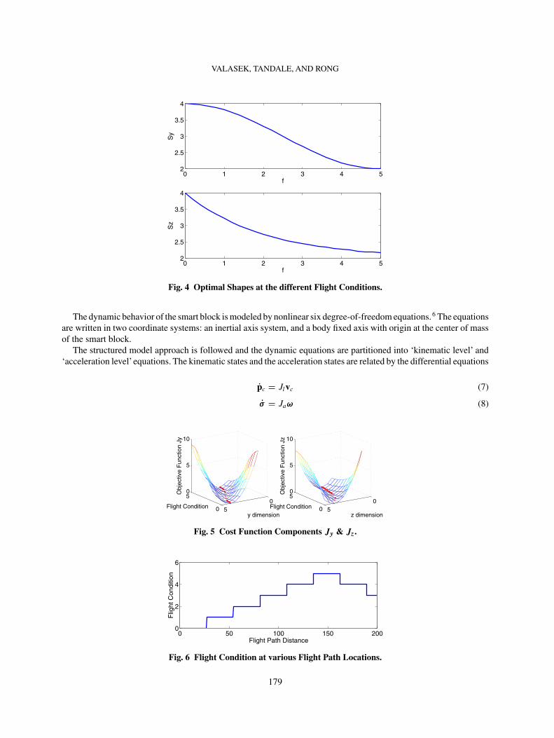
The total cost function J can be written as a sum J = Jy + Jz. The optimal shapes are arbitrarily selected to benonlinear functions of the flight condition and are shown graphically in Fig. 4.

Sy = 3+ cos(π

5f

)(3)

Sz = 2+ 2e−0.5f (4)

−2

−1

0

1

2

−2

−1

0

1

2−1

−0.5

0

0.5

1

XY

Z

Fig. 1 Shape of the morphing smart block.

177


0 1 2 3 4 52

2.5

3

3.5

4

Voltage − Vyy

dim

ensi

on

0 0.5 1 1.5 2 2.5 3 3.5 42

2.5

3

3.5

4

Voltage − Vz

z di

men

sion

Fig. 2 The Steady State Dimensions corresponding to the Applied Voltage.

With the optimal y dimension given by Eq. 3, the cost function Jy is defined as

Jy = (y − Sy(f ))2 (5)

The surface plot of Jy is shown in Fig. 5. Similarly, the cost function Jz is defined as

Jz = (z− Sz(f ))2 (6)

The surface plot of Jz is shown in Fig. 5. For the simulation we specify the flight conditions that the smart blockshould fly at various locations along a pre-designated flight path (Fig. 6). For this preliminary example the optimalshapes are not correlated to the flight path, but depend only on the flight condition.

The objective of the Reinforcement Learning Module is to learn the control policy that, for a specific flightcondition, commands the voltage which produces the optimal shapeSy andSz. Therefore, the Reinforcement Learningmodule seeks to minimize the total cost J over the entire flight trajectory.

A. Mathematical Model for the Dynamic Behavior of the Smart BlockThe dynamic behavior of the smart block is like a hovering air vehicle. The simulation assumes absence of gravity.

The vehicle has thrusters along all three axis which act as the control effectors. Note that the total velocity vector ofthe vehicle can point in any arbitrary direction.

0 5 101.5

2

2.5

3

3.5

4

4.5

Time (sec)

y di

men

sion

0 5 102

2.5

3

3.5

4

4.5

Time (sec)

z di

men

sion

Fig. 3 The Morphing Dynamics for y and z dimensions when subjected to various input voltages Vy and V z.

178


0 1 2 3 4 52

2.5

3

3.5

4

f

Sy

0 1 2 3 4 52

2.5

3

3.5

4

f

Sz

Fig. 4 Optimal Shapes at the different Flight Conditions.

The dynamic behavior of the smart block is modeled by nonlinear six degree-of-freedom equations.6 The equationsare written in two coordinate systems: an inertial axis system, and a body fixed axis with origin at the center of massof the smart block.

The structured model approach is followed and the dynamic equations are partitioned into ‘kinematic level’ and‘acceleration level’equations. The kinematic states and the acceleration states are related by the differential equations

pc = Jlvc (7)

σ = Jaω (8)

0

50

5

0

5

10

y dimensionFlight Condition

Obj

ectiv

e F

unct

ion

Jy

0

50

5

0

5

10

z dimensionFlight Condition

Obj

ectiv

e F

unct

ion

Jz

Fig. 5 Cost Function Components Jy & Jz.

0 50 100 150 2000

2

4

6

Flight Path Distance

Flig

ht C

ondi

tion

Fig. 6 Flight Condition at various Flight Path Locations.

179


where

Jl =CθCψ SφSθCψ − CφSψ CφSθCψ + SφSψCθSψ SφSθSψ + CφCψ CφSθSψ − SφCψ−Sθ SφCθ CφCθ

Ja =1 Sφtan(θ) Cφtan(θ)

0 Cφ −Sφ0 Sφsec(θ) Cφsec(θ)

(9)

The acceleration level differential equations are

mvc + ωmvc = F+ Fd (10)

I ω + Iω + ωIω =M+Md (11)

ω = 0 −r q

r 0 −p−q p 0

(12)

Note that for this study the motion of the smart block is simulated in the absence of gravity. Also Eq. 11 has anadditional term Iω, when compared to rigid body equations of motion. This term is a consequence of the shapechange and is responsible for speeding up or slowing down the rotation of the block due to the time rate of changein the moment of inertia about a particular axis.

The drag force Fd is modeled as a function of the air density ρ, the square of the velocity along the axis and thearea of the smart block perpendicular to the axis.

Fd = −ρ2

u2sgn(u)yz

v2sgn(v)xz

w2sgn(w)xy

(13)

Similarly, the drag moment Md is modeled as a function of the air density ρ, the square of the angular velocity alongthe axis and the area of the surfaces of the smart block parallel to the axis.

Md = −ρ2

p2sgn(p)x(y + z)q2sgn(q)y(x + z)r2sgn(r)z(x + y)

(14)

B. Trajectory GenerationThe reference trajectory is arbitrary and is generated as a combination of straight lines and sinusoidal curves.

Fig. 7 shows a sample reference trajectory that the smart block is required to track. The total flight path is divided intoan odd number of segments of variable lengths. During every odd numbered segment the Y and Z locations remain

0

20

40

60

80

100

050

5

X (m)

Y (m)

Z (

m)

Fig. 7 Reference Trajectory for Positions along Inertial Axis.

180


0 20 40 60 80 1000

2

4

X (m)

Y (

m)

0 50

2

4

Y (m)

Z (

m)

0 20 40 60 80 1000

2

4

X (m)

Z (

m)

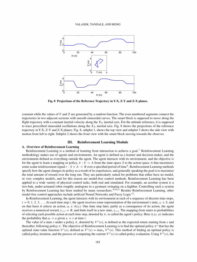
Fig. 8 Projections of the Reference Trajectory in Y-X, Z-Y and Z-X planes.

constant while the values of Y and Z are generated by a random function. The even numbered segments connect thetrajectories in two adjacent sections with smooth sinusoidal curves. The smart block is supposed to move along theflight trajectory with a constant inertial velocity along the XN inertial axis. For the attitude reference, it is supposedto trace prescribed sinusoidal oscillations along the XN inertial axis. Fig. 8 shows the projections of the referencetrajectory in Y-X, Z-Y and Z-X planes. Fig. 8, subplot 1, shows the top view and subplot 3 shows the side view withmotion from left to right. Subplot 2 shows the front view with the smart block moving towards the observer.

III. Reinforcement Learning ModuleA. Overview of Reinforcement Learning

Reinforcement Learning is a method of learning from interaction to achieve a goal.7 Reinforcement Learningmethodology makes use of agents and environments. An agent is defined as a learner and decision-maker, and theenvironment defined as everything outside the agent. The agent interacts with its environment, and the objective isfor the agent to learn a mapping or policy, π : S → A from the state-space S to the action space A that maximizessome scalar reinforcement signal r : S × A→ R over a specified period of time8. Reinforcement Learning methodsspecify how the agent changes its policy as a result of its experiences, and generally speaking the goal is to maximizethe total amount of reward over the long run. They are particularly suited for problems that either have no model,or very complex models, and for this reason are model-free control methods. Reinforcement Learning has beenapplied to a wide variety of physical control tasks, both real and simulated. For example, an acrobat system is atwo-link, under-actuated robot roughly analogous to a gymnast swinging on a highbar. Controlling such a systemby Reinforcement Learning has been studied by many researchers.9,10,11 Besides Reinforcement Learning, othermodel-free control approaches include artificial Neural Networks and Fuzzy Logic12.

In Reinforcement Learning, the agent interacts with its environment at each of a sequence of discrete time steps,t = 0, 1, 2, 3, . . .. At each time step t , the agent receives some representation of the environment’s state, st ∈ S, andon that basis it selects an action, at ∈ A(st ). One time step later, partly as a consequence of its action, the agentreceives a numerical reward, rt+1 = R, and finds itself in a new state, st+1. The mapping from states to probabilitiesof selecting each possible action at each time step, denoted by π , is called the agent’s policy. Here πt(s, a) indicatesthe probability that at = a given st = s at time t .

The value of a state s under a policy π , denoted by V π(s), is defined as the expected return starting from s andthereafter, following policy π . The objective of Reinforcement Learning is to find the optimal policy π∗ that has theoptimal state-value function V ∗(s), defined as V ∗(s) = maxπ V π(s). This method of finding an optimal policy iscalled policy iteration, and the process of computing the current V π(s) is called policy evaluation. Using V π(s), the

181


policy π can then be improved to policy π ′, and this process is called policy improvement. Finally, V π′(s) can then

be used in successive iterations to compute a yet more improved policy, π ′′.There are three major methods for policy iteration: Dynamic Programming, Monte Carlo methods, and Temporal-

Difference learning. Dynamic Programming refers to a collection of algorithms that can be used to compute optimalpolicies given a perfect model of the environment as a Markov decision process (MDP). The key idea is the use ofvalue functions to organize and structure the search for good policies. Classical Dynamic Programming algorithms13,14,15 are of limited utility in Reinforcement Learning, both because of their assumption of a perfect model and theirgreat computational expense. However, they are very important theoretically. Monte Carlo methods are employedto estimate functions using an iterative, incremental procedure. The term “Monte Carlo” is sometimes used morebroadly for any estimation method whose operation involves a significant random component. For the present contextit represents methods which solve the Reinforcement Learning problem based on averaging sample returns. To ensurethat well-defined returns are available, they are defined only for episodic tasks, and it is only upon the completion ofan episode that value estimates and policies are changed. By comparison with Dynamic Programming, Monte Carlomethods can be used to learn optimal behavior directly from interaction with the environment, with no model of theenvironment’s dynamics. They can be used with simulation, and it is easy and efficient to focus Monte Carlo methodson a small subset of the states. All Monte Carlo methods for Reinforcement Learning have been developed onlyrecently, and their convergence properties are not well understood. Temporal-Difference methods can be viewed as anattempt to achieve much the same effect as Dynamic Programming, but with less computation and without assuminga perfect model of the environment. Sutton’s method of Temporal-Differences is a form of the policy evaluationmethod in Dynamic Programming in which a control policy π0 is to be chosen16. The prediction problem becomesthat of learning the expected discounted rewards, V π(i), for each state i in S using π0. With the learned expecteddiscounted rewards, a new policy π1 can be determined that improves upon π0. The algorithm may eventuallyconverge to some policy under this iterative improvement procedure, as in Howard’s algorithm.17 Q-Learning isa form of the successive approximations technique of Dynamic Programming, first proposed and developed byWatkins.18 Q-learning learns the optimal value functions directly, as opposed to fixing a policy and determining thecorresponding value functions, like Temporal-Differences. It automatically focuses attention to where it is needed,thereby avoiding the need to sweep over the state-action space. Additionally, it is the first provably convergent directadaptive optimal control algorithm.

In many applications of Reinforcement Learning to control tasks, the state space is too large to enumerate thevalue function so function approximators must be used to compactly represent it. For example, tile coding has beenused in many Reinforcement Learning systems.19,20,21,22 Other commonly used approaches include neural networks,clustering, nearest-neighbor methods and cerebellar model articulator controller.

B. Implementation of Reinforcement Learning ModuleFor the present research, the agent in the smart block problem is its Reinforcement Learning module, which

attempts to minimize the total amount of cost over the entire flight trajectory. To reach this goal, it endeavors to learn,from its interaction with the environment, the optimal policy that, given the specific flight condition, commandsthe voltage that changes the smart block’s shape to the optimal one. The environment is the flight conditions whichthe smart block is flying in, along with its shape. We assume that the Reinforcement Learning module has no priorknowledge of the relationship between voltages and the dimensions of the block, as defined by morphing controlfunctions in Eq. 1 and Eq. 2. Also it does not know the relationship between the flight conditions, costs and theoptimal shapes as defined in Eq. 4 to Eq. 6. However, the Reinforcement Learning module does know all possiblevoltages that can be applied. It has accurate, real-time information of the smart block’s shape, the present flightcondition, and the current cost provided by a variety of sensors.

The Reinforcement Learning module learns the state value function using Actor-Critic methods.7 These areclassical Temporal-Difference learning methods that utilize two parametric structures, one called the actor, and theother called the critic. The actor consists of a parameterized control law or policy function, which is used to selectactions. The critic approximates a value function that is used to critique the actions made by the actor, therebycapturing the effect that the policy function will have on the future cost. At any given time, the critic providesguidance on how to improve the policy function. In return, the actor can be used to update the critic. An algorithm

182


that successively iterates between these two operations will converge to the optimal solution over time. An Actor-Critic method is selected for the current research primarily for convenience of implementation and evaluation, dueto it’s separate memory structure to explicitly represent the policy, independent of the value function. Since twoseparate modules are used to represent value functions and policies, modifications to one module (different typesof action sets, state-spaces, and reward functions) can be made without affecting the other module. Additionally,Actor-Critic methods are able to handle problems with a continuous state-space. One way to do this (shown below)is to use linear function approximation methods. A parameterized functional form with a parameter vector is used torepresent the value functions in the Critic, and the action preference functions in the Actor. Central to the operationof the Actor-Critic method is the Temporal-Difference error defined in Eq. 15, which is used to determine whetheran action is better or worse than expected.

δt = rt+1 + γV (st+1)− V (st ) (15)

At the same time, the critic updates its current estimated value function using the Temporal-Difference error

V (st )← V (st )+ δt (16)

In Eq. 15, V is the current estimated value function used by the critic. If the Temporal-Difference error is positive,it suggests that the tendency to select at when in state st should be strengthened for the future. If the Temporal-Difference error is negative, it suggests that the tendency should be weakened. The policy implemented by the actoris based on the preference functions, p(s, a) which indicate the tendency to select each a when in each state s.Example policies are, the greedy policy

πt(s, a) = argmaxap(s, a) (17)

and the Gibbs softmax policy7

πt(s, a) = Pr{at = a|st = s} = ep(s,a)∑a e

p(s,a)(18)

The strengthening or weakening tendency described above is implemented by increasing or decreasing p(st , at ),for instance, using

p(st , at )← p(st , at )+ βδt (19)

As shown in the Morphing Smart Block Simulation section, for this research the dimensions of the morphing blockare continuous. Therefore, the morphing block has a continuous state-space, and its state-value function V π(s) andaction-preference function Pat (s) are both defined on continuous domains. One approach to solving this type ofReinforcement Learning problem with a continuous state-space is function approximation methods. In the presentexample, the approximate state-value function V π(s) is represented using a parameterized functional form withparameter vector θv

V π(s) =N∑j=1

θvj�j (s), ∀s ∈ S (20)

where �j(s) is predetermined and satisfies

�i(s) ·�j(s) ={

1 if i = j0 if i �= j

}(21)

Thus the basis vector

H = [�i(s) �2(s) . . . �N(s)

]T(22)

is an orthogonal vector that satisfies

HHT = IN×N (23)

183


Using Eq. 22, Eq. 20 becomes

V π(s) = HT θv, ∀s ∈ S (24)

AsHT is fixed,V π(s) depends totally on θv , and varies from time step to time step only when θv changes. Updatingθv is related to the Temporal-Difference error δt as defined in Eq. 15. The process of deriving the updating formulafor θv is shown as follows: First, we selected the gradient descent method for updating V (st ), upon which Eq. 16becomes

V (st )← V (st )+ αδt (25)

Using Eq. 24, Eq. 25 becomes

HTt θv ← HT

t θv + αδt (26)

whereHt =[�1(st ) �2(st ) . . . �N(st )

], andHt is the known coefficient matrix. Using Eq. 23, the formula for

updating θv becomes

θv ← θv + αδtHt (27)

Note that the purpose of the Reinforcement Learning module is not to compute the exact V π(s), but to learn theoptimal policy π∗ with the optimal state-value function V ∗(s). In the process of policy iteration, an intermediatepolicy π can be improved to a better policy π ′ even if its state-value function V π(s) is not exactly computed.

Similarly for the actor, the preference function for each action is represented using a parameterized functionalform with parameter vector θpa .

pa(s) = HT θpa (28)

Since V (s) and pa(s) are both defined on the same state-space, the basis vector H can also be used for V (s). UsingEq. 19, and following a similar process from Eq. 25 to Eq. 27, the formula for updating θpa is

θpa ← θpa + αβδtHTt (29)

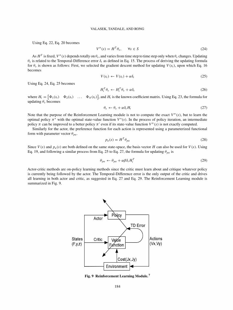
Actor-critic methods are on-policy learning methods since the critic must learn about and critique whatever policyis currently being followed by the actor. The Temporal-Difference error is the only output of the critic and drivesall learning in both actor and critic, as suggested in Eq. 27 and Eq. 29. The Reinforcement Learning module issummarized in Fig. 9.

Fig. 9 Reinforcement Learning Module.7

184


The Reinforcement Learning agent always encounters an exploration-exploitation dilemma when it selects thenext action given its current state7. If it selects a greedy action that has the highest preference for the current state,then it is exploiting its knowledge obtained so far, about the values of the actions. If instead it selects one of thenon-greedy actions, then it is exploring to improve its estimate of the non greedy actions’ values. In the early stage ofthe learning, the Reinforcement Learning agent employs a uniform probability policy under which each action hasthe same probability to be selected. In this way it can explore as many states and actions as possible. In the middlestage, it changes to a Gibbs Softmax Policy as described in Eq. 18, under which the actions with a higher preferencehave higher probability to be selected. Using this policy allows the module to partially explore and partially exploitat the same time. In the final stage, it uses a greedy policy, as described in Eq. 17, that allows it to totally exploit itsprevious experience.

IV. Structured Adaptive Model InversionA. A Brief Introduction to Structured Adaptive Model Inversion (SAMI)

The goal of the SAMI controller is to track the reference trajectories, even when the dynamic properties of thesmart block change, due to the morphing. Structured Adaptive Model Inversion (SAMI)23 is based on the concepts ofFeedback Linearization24, Dynamic Inversion, and Structured Model Reference Adaptive Control (SMRAC).25,26,27

In SAMI, dynamic inversion is used to solve for the control. The dynamic inversion is approximate, as the systemparameters are not modeled accurately. An adaptive control structure is wrapped around the dynamic inverter toaccount for the uncertainties in the system parameters.28,29,30 This controller is designed to drive the error betweenthe output of the actual plant and that the reference trajectories to zero, with prescribed error dynamics. Mostdynamic systems can be represented as two sets of differential equations, an exactly known kinematic level part, anda momentum level part with uncertain system parameters. The adaptation included in this framework can be limitedto only the uncertain momentum level equations, thus restricting the adaptation only to a subset of the state-space,enabling efficient adaptation. SAMI has been shown to be effective for tracking spacecraft31 and aggressive aircraftmaneuvers32. The SAMI approach has been extended to handle actuator failures and to facilitate correct adaptationin presence of actuator saturation.33,34,35

B. Mathematical Formulation of the SAMI Controller for Attitude ControlThe attitude equations of motion for the smart block are given by Eq. 8 and Eq. 11. Without the angular drag and

the Iω term, Eq. 8 and Eq. 11 can be manipulated to obtain the following form23

I ∗a (σ )σ + C∗a (σ , σ )σ = PTa (σ )M (30)

where the matrices I ∗a (σ ), C∗a (σ, σ ) and P(σ) are defined as

Pa(σ ) � J−1a (σ ) (31)

I ∗a (σ ) � PTa IPa (32)

C∗a (σ, σ ) � −I ∗a JaPa + PTa [Paσ ]IPa (33)

The left hand side of Eq. 30 can be linearly parameterized as follows

I ∗a (σ )σ + C∗a (σ , σ )σ = Ya(σ , σ , σ )� (34)

where and � is defined as � �[I11 I22 I33 I12 I13 I23

]T. It can be seen that the product of the inertia matrix

and a vector can be written as

Iν = (ν)�, ∀ν ∈ R3 (35)

where ∈ R3×6 is defined as

(ν) �

ν1 0 0 ν2 ν3 0

0 ν2 0 ν1 0 ν3

0 0 ν3 0 ν1 ν2

(36)

185


The terms on the left hand side of Eq. 30 can be written as

I ∗a σ = PTa IPa σ= PTa (Pa σ )� (37)

C∗a σ = −PTa IPaJaPa σ + PTa [Pa σ ]IPa σ= PTa {− (PaJaPa σ )+ [Pa σ ] (Pa σ )}� (38)

Combining Eqs. 37 and 38 we have the linear minimal parametrization for the inertia matrix36.

I ∗a (σ )σ + C∗a (σ , σ )σ= PTa { (Pa σ )− (PaJaPa σ )+ [Pa σ ] (Pa σ )}�= Ya(σ , σ , σ )� (39)

The attitude tracking problem can be formulated as follows. The control objective is to track an attitude trajectoryin terms of the 3-2-1 Euler angles. The desired reference trajectory is assumed to be twice differentiable with respectto time. Let ε � σ -σr be the tracking error. Differentiating twice and multiplying by I ∗a throughout

I ∗a ε = I ∗a σ − I ∗a σr (40)

Adding (Cda + C∗(σ , σ ))ε + Kda ε on both sides,

I ∗a ε + (Cda + C∗a (σ , σ ))ε +Kdaε = I ∗a σ − I ∗a σr + (Cda + C∗a (σ , σ ))ε +Kdaε (41)

The RHS of Eq. 41 can be written as

(I ∗a σ + C∗a (σ , σ )σ )− (I ∗a σr + C∗a (σ , σ )σr)+ Cda ε +Kdaε (42)

From Eq. 30 and the construction of Y similar to Eq. 39, the RHS of Eq. 41 can be further written as

PTa M− Ya(σ , σ , σr , σ r )�+ Cda ε +Kdaε (43)

So the control law can be now chosen as

M = P−Ta {Ya(σ , σ , σr , σ r )�− Cda ε −Kdaε} (44)

The above control law requires that the inertia parameters � be known accurately, but they may not be knownaccurately in actual practice. So by using the certainty equivalence principle30, adaptive estimates for the inertiaparameters � will be used for calculating the control.

M = P−Ta {Ya(σ , σ , σr , σ r )�− Cda ε −Kdaε} (45)

With the control law given in Eq. 45 the closed loop dynamics takes the following form

I ∗a ε + (Cda + C∗a (σ , σ ))ε +Kdaε = Ya(σ , σ , σ )� (46)

where � = �−�. The update for the parameter � and the stability proof can be obtained by doing a Lyapunovanalysis.

186


Consider the candidate Lyapunov function

V = 1

2εTI ∗a ε +

1

2εT Kdaε + 1

2�Tτ−1� (47)

Taking the derivative of the Lyapunov function along the closed loop trajectories given by Eq. 46

V = 1

2εTI ∗a ε + ε

TI ∗a ε + ε

TKdaε + 1

2˙�T

τ−1� (48)

which can be simplified as

V = εT [1

2I ∗a − C∗a ]ε − ε

TCda ε + (εT Ya(σ , σ , σr , σ r )+ ˙

�T

τ−1)� (49)

The first term vanishes because [ 12 I ∗a − C∗a ] is skew symmetric. Setting the coefficient of � to 0, to obtain the adaptivelaws.

˙� = −τYa(σ , σ , σr , σ r )

T ε (50)

From the definition of � and assuming that the true parameter � remains constant,

˙� = −τYa(σ , σ , σr , σ r )

T ε (51)

This update law renders the derivative of the Lyapunov function

V = −εTCda ε (52)

Thus the derivative is negative semi definite. From Eq. 47 and Eq. 52 it can be concluded that ε,ε and � are bounded.Using the standard procedure of application of Barbalat’s lemma30,37, asymptotic stability of the tracking errordynamics can be concluded for bounded reference trajectories.

C. Mathematical Formulation of the SAMI Controller for Control of Linear StatesFollowing similar lines as the attitude controller, Eq. 7 and Eq. 10, without the drag term can be cast in the

following form

I ∗l pc + C∗l pc = PTl F (53)

where the matrices I ∗l , C∗l and Pl are defined as

Pl � J−1l (54)

I ∗l � PTl mPl (55)

C∗l � −I ∗l JlPl + PTl ωmPl (56)

The control law with the adaptive parameter m is

F = P−Tl {Ylm− Cdl ε −Kdlε} (57)

where

Yl = PTl Pl pc(ref ) − PTl PlJlPl pc(ref ) + PTl ωPl pc(ref ) (58)

Subscript (ref ) indicates the respective reference state and ε� pc − pc(ref ) is the tracking error for the linear position.The update law for the adaptive parameter m is

˙m = −�YTl ε (59)

187


V. A-RLC Architecture FunctionalityThe Adaptive-Reinforcement Learning Control Architecture is composed of two sub-systems: Reinforcement

Learning and Structured Adaptive Model Inversion (SAMI) (Fig. 10). The two sub-systems interact significantlyduring both the episodic learning stage, when the optimal shape change policy is learned, and the operational stage,when the plant morphs and tracks a trajectory. For either type of stage, the system functions as follows.

Considering the Reinforcement Learning sub-system at the top of Fig. 10 and moving counterclockwise, theReinforcement Learning module initially commands an arbitrary action from the set of admissible actions. Thisaction is sent to the plant, which produces a shape change. The cost associated with the resultant shape changein terms of system states, parameters, and user defined performance measures, is evaluated with the cost functionand then passed to the Critic. The Critic calculates the Temporal-Difference error using its current estimated statevalue function, which is sent to the Actor. The Critic modifies it’s state value function according to the Temporal-Difference error, and likewise the Actor updates it’s action preference function. For the next episode, the Actorgenerates a new action based on the current policy and its updated action preference function, and the sequencerepeats itself.

Considering the SAMI sub-system at the bottom of Fig. 10, shape changes in the plant due to actions generatedby the Actor cause the plant dynamics to change. The SAMI controller maintains trajectory tracking irrespective ofthe changing dynamics of the plant due to these shape changes.

Fig. 10 Adaptive-Reinforcement Learning Control Architecture.

188


VI. Numerical ExampleA. Purpose and Scope

The purpose of the numerical example is to demonstrate the learning performance and the trajectory trackingperformance of the A-RLC architecture. To learn the optimal shape change policy a total of 200 learning episodesare used, each consisting of a single 200 second transit through a 100 meter long path. The reference trajectory tobe tracked in each episode is generated arbitrarily. The sequence of the flight conditions is random, and changestwice during each episode. At a particular flight condition the Reinforcement Learning Module commands arbitraryvoltages at ten second intervals, that result in the corresponding shape and records the cost expended due to thatshape. Thus it builds up its knowledge base and learns the optimal shape change policy.

After the learning episodes are complete, the learned knowledge of the Reinforcement Learning Module andthe trajectory tracking capability of the SAMI Controller have to be evaluated. These are evaluated with a singlepass through the path, with a randomly generated reference trajectory and an arbitrary flight condition change atapproximately 50 second intervals. Fig. 6 shows a typical flight condition sequence.

B. Learning the Optimal Policy for Shape ChangeFor the definitions of the morphing control functions and the cost functions defined by Eq. 1 to Eq. 5, this

Reinforcement Learning problem can be decoupled into two independent problems that correspond to the y and zdimensions respectively. For the y dimension Reinforcement Learning problem, the state has two elements: the valueof y dimension and the flight condition s = {y, f }. The state set consisting of all possible states is a 2-Dimensionalcontinuous Cartesian space S = [2, 4] × [0, 5]. For each state, the action set consists all possible voltages that can beapplied A(s) = {0, 0.5, 1, 1.5, 2, 2.5, 3, 3.5, 4, 4.5, 5}. Similarly for the z dimension, the state set is [2, 4] × [0, 5],and the action set is {0, 0.5, 1, 1.5, 2, 2.5, 3, 3.5, 4}. Note that the control can take only the discrete values shownabove.

For simplicity, the training is conducted only at six discrete flight conditions{0, 1, 2, 3, 4, 5}. For the functionapproximation for V πt (s) and pat (s), a relatively simple linear approximation method was used: tile coding. Thebasis function �j(s)is defined as follows

�j(s) ={

1 if (s − cj )TR−1(s − cj ) ≤ 10 if (s − cj )TR−1(s − cj ) > 1

(60)

For the y dimension, the set of all center state vectors is 2-dimensional,Cy = y × f , where f = {0, 1, 2, 3, 4, 5},and Cy has 102 total elements. The weighting matrix R−1 is defined as

R−1 =[r2

1 00 r2

2

]−1

r1 = 0.1, r2 = 0.0625 (61)

In tile coding, the basis function�j is called a binary feature or a tile. One advantage of tile coding is the capabilityof controlling the overall features which are activated at one time. In the present case, only one feature is present atone time. For the z dimension, the tile �j(s), the center state vector set Cz = z× f , and the weighting matrix R−1

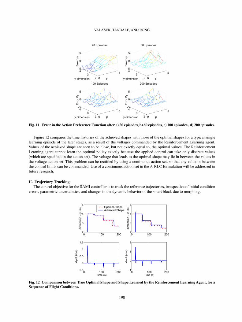
are defined in the same fashion.Fig. 11 is a graphical representation of the errors in the preferred voltages of the y-dimension selected by theActor,

when compared with the true values used for simulation. The preferred voltages are calculated based on the policy andthe estimated action preference functions currently used.As the learning progresses from 20 to 200 episodes, the errorplot becomes flatter and the errors at more points converge to zero. This indicates that the action preference functionsare being learned accurately. The decrease in error is less significant from 100 to 200 episodes than from 20 to 60episodes, since the focus shifts from exploration to exploitation, and the action preference functions asymptoticallyconverge to those of the optimal policy. Note that the error at y = 3.5 appears to increase with successive episodes.This point in the state-space has only been visited at flight condition 1 within 200 episodes, and not at any otherflight condition. Since a function approximation is being used, extrapolation is occurring and may give rise to anincorrect voltage, and therefore nonzero error. With a finer resolution of discrete voltages in the action set, thiswould not occur. However, here it does not affect the results since that point is never visited in this example (seeFig. 3).

189


0

5

23

4−5

0

5

F

20 Episodes

y dimensionE

rror

Vy

0

5

23

4−5

0

5

F

60 Episodes

y dimension

Err

or V

y

0

5

23

4−5

0

5

F

100 Episodes

y dimension

Err

or V

y

0

5

23

4−5

0

5

F

200 Episodes

y dimension

Err

or V

yFig. 11 Error in the Action Preference Function after a) 20 episodes, b) 60 episodes, c) 100 episodes , d) 200 episodes.

Figure 12 compares the time histories of the achieved shapes with those of the optimal shapes for a typical singlelearning episode of the later stages, as a result of the voltages commanded by the Reinforcement Learning agent.Values of the achieved shape are seen to be close, but not exactly equal to, the optimal values. The ReinforcementLearning agent cannot learn the optimal policy exactly because the applied control can take only discrete values(which are specified in the action set). The voltage that leads to the optimal shape may lie in between the values inthe voltage action set. This problem can be rectified by using a continuous action set, so that any value in betweenthe control limits can be commanded. Use of a continuous action set in the A-RLC formulation will be addressed infuture research.

C. Trajectory TrackingThe control objective for the SAMI controller is to track the reference trajectories, irrespective of initial condition

errors, parametric uncertainties, and changes in the dynamic behavior of the smart block due to morphing.

0 100 2002

3

4

5

dim

ensi

on −

y (

m) Optimal Shape

Achieved Shape

0 100 2002

3

4

5

dim

ensi

on −

z (

m)

0 100 200−0.5

0

0.5

1

1.5

Time (s)

dy/d

t (m

/s)

0 100 200−1

0

1

2

Time (s)

dz/d

t (m

/s)

Fig. 12 Comparison between True Optimal Shape and Shape Learned by the Reinforcement Learning Agent, for aSequence of Flight Conditions.

190


0 20 40 60 80 1000

2

4

X (m)

Y (

m)

Actual TrajectoryReference

0 50

2

4

Y (m)

Z (

m)

0 20 40 60 80 1000

2

4

X (m)

Z (

m)

Fig. 13 Projections of the Trajectory in Y-X, Z-Y and Z-X planes.

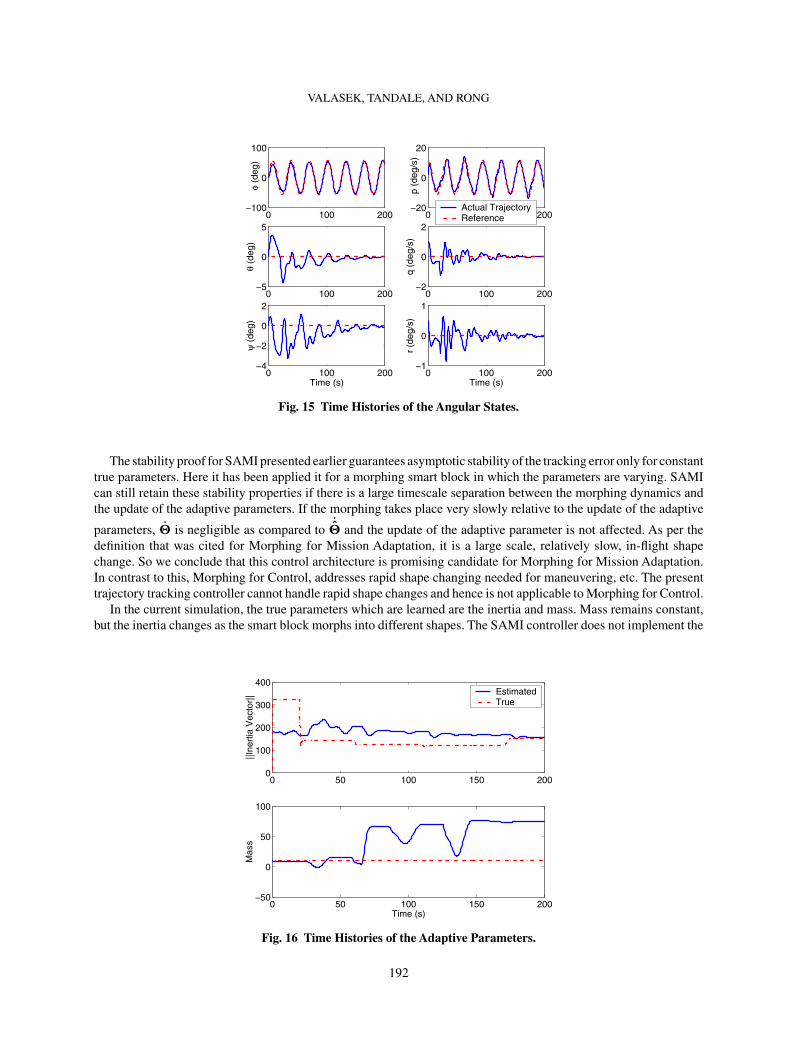
Figure 13 shows that the adaptive control maintains close tracking of the reference trajectories. Figure 14 andFig. 15 show the time histories of the linear and angular states respectively. The deviations from the referencetrajectory for the linear velocities v and w seen in Fig. 14, are due to rapid changes in the smart block’s dimensions.Also note that the vehicle has displacements along y and z inertial axes with commanded pitch and yaw angles zero.Since the conceptual air vehicle has thrusters on all three axes and is capable of hover, total velocity can be in anyarbitrary direction.

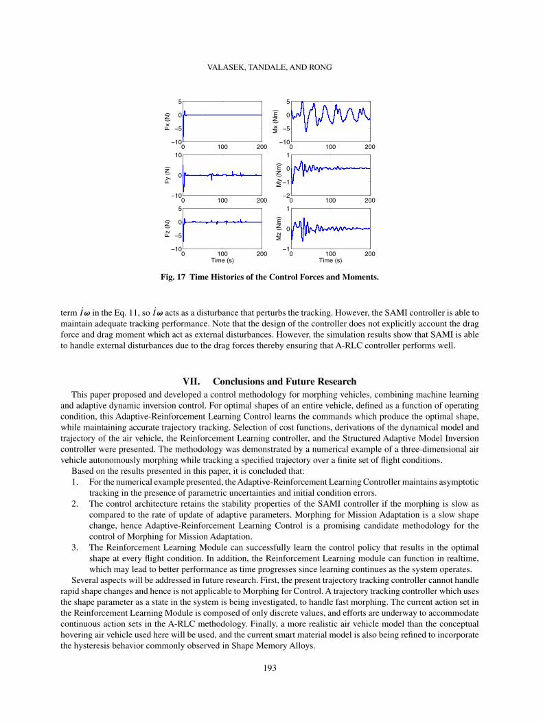
Figure 16 shows the variation in the true parameters and the update of the adaptive parameters. The adaptiveparameters do not converge to the true parameters, which is commonly seen in adaptive control systems. Theparameters only converge to the true values if the reference trajectory is persistently exciting. 30 Most importantly,Fig.16 shows that the adaptive parameters are bounded, and do not diverge. Figure 17 shows that the control forcesand moments are well behaved.

0 100 2000

50

100

150

X (

m)

0 100 2002

3

4

5

Y (

m)

0 100 2000

2

4

6

Z (

m)

Time (s)

0 100 2000

0.5

1

1.5

u (m

/s)


0 100 200−1

0

1

2

v (m

/s)

0 100 200−1

0

1

2

w (

m/s

)

Time (s)

Fig. 14 Time Histories of the Linear States.

191


0 100 200−100

0

100

φ (d

eg)

0 100 200−5

0

5

θ (d

eg)

0 100 200−4

−2

0

2

ψ (

deg)

Time (s)

0 100 200−20

0

20

p (d

eg/s

)


0 100 200−2

0

2

q (d

eg/s

)

0 100 200−1

0

1

r (d

eg/s

)

Time (s)

Fig. 15 Time Histories of the Angular States.

The stability proof for SAMI presented earlier guarantees asymptotic stability of the tracking error only for constanttrue parameters. Here it has been applied it for a morphing smart block in which the parameters are varying. SAMIcan still retain these stability properties if there is a large timescale separation between the morphing dynamics andthe update of the adaptive parameters. If the morphing takes place very slowly relative to the update of the adaptive

parameters, � is negligible as compared to ˙� and the update of the adaptive parameter is not affected. As per the

definition that was cited for Morphing for Mission Adaptation, it is a large scale, relatively slow, in-flight shapechange. So we conclude that this control architecture is promising candidate for Morphing for Mission Adaptation.In contrast to this, Morphing for Control, addresses rapid shape changing needed for maneuvering, etc. The presenttrajectory tracking controller cannot handle rapid shape changes and hence is not applicable to Morphing for Control.

In the current simulation, the true parameters which are learned are the inertia and mass. Mass remains constant,but the inertia changes as the smart block morphs into different shapes. The SAMI controller does not implement the

0 50 100 150 2000

100

200

300

400

||Ine

rtia

Vec

tor|

| EstimatedTrue

0 50 100 150 200−50

0

50

100

Mas

s

Time (s)

Fig. 16 Time Histories of the Adaptive Parameters.

192


0 100 200−10

−5

0

5

Fx

(N)

0 100 200−10

0

10

Fy

(N)

0 100 200−10

−5

0

5

Fz

(N)

Time (s)

0 100 200−10

−5

0

5

Mx

(Nm

)

0 100 200−2

−1

0

1

My

(Nm

)

0 100 200−1

0

1

Mz

(Nm

)

Time (s)

Fig. 17 Time Histories of the Control Forces and Moments.

term Iω in the Eq. 11, so Iω acts as a disturbance that perturbs the tracking. However, the SAMI controller is able tomaintain adequate tracking performance. Note that the design of the controller does not explicitly account the dragforce and drag moment which act as external disturbances. However, the simulation results show that SAMI is ableto handle external disturbances due to the drag forces thereby ensuring that A-RLC controller performs well.

VII. Conclusions and Future ResearchThis paper proposed and developed a control methodology for morphing vehicles, combining machine learning

and adaptive dynamic inversion control. For optimal shapes of an entire vehicle, defined as a function of operatingcondition, this Adaptive-Reinforcement Learning Control learns the commands which produce the optimal shape,while maintaining accurate trajectory tracking. Selection of cost functions, derivations of the dynamical model andtrajectory of the air vehicle, the Reinforcement Learning controller, and the Structured Adaptive Model Inversioncontroller were presented. The methodology was demonstrated by a numerical example of a three-dimensional airvehicle autonomously morphing while tracking a specified trajectory over a finite set of flight conditions.

Based on the results presented in this paper, it is concluded that:1. For the numerical example presented, theAdaptive-Reinforcement Learning Controller maintains asymptotic

tracking in the presence of parametric uncertainties and initial condition errors.2. The control architecture retains the stability properties of the SAMI controller if the morphing is slow as

compared to the rate of update of adaptive parameters. Morphing for Mission Adaptation is a slow shapechange, hence Adaptive-Reinforcement Learning Control is a promising candidate methodology for thecontrol of Morphing for Mission Adaptation.

3. The Reinforcement Learning Module can successfully learn the control policy that results in the optimalshape at every flight condition. In addition, the Reinforcement Learning module can function in realtime,which may lead to better performance as time progresses since learning continues as the system operates.

Several aspects will be addressed in future research. First, the present trajectory tracking controller cannot handlerapid shape changes and hence is not applicable to Morphing for Control. A trajectory tracking controller which usesthe shape parameter as a state in the system is being investigated, to handle fast morphing. The current action set inthe Reinforcement Learning Module is composed of only discrete values, and efforts are underway to accommodatecontinuous action sets in the A-RLC methodology. Finally, a more realistic air vehicle model than the conceptualhovering air vehicle used here will be used, and the current smart material model is also being refined to incorporatethe hysteresis behavior commonly observed in Shape Memory Alloys.

193


AcknowledgmentsThe authors wish to acknowledge the support of the Texas Institute for Intelligent Bio-Nano Materials and

Structures for Aerospace Vehicles. The material is based upon work supported by NASA under award no. NCC-1-02038. Any opinions, findings, and conclusions or recommendations expressed in this material are those of theauthor(s) and do not necessarily reflect the views of the National Aeronautics and Space Administration. The authorsthank the Associate Editor and reviewers for their many insightful comments and suggestions, which improved thepaper.

References1Wlezien, R., Horner, G., McGowan, A., Padula, A., Scott, M., Silcox, R., and Simpson, J., “The Aircraft Morphing Program,”

No. AIAA-98-1927.2McGowan, A.-M. R., Washburn, A. E., Horta, L. G., Bryant, R. G., Cox, D. E., Siochi, E. J., Padula, S. L., and Holloway,

N. M., “Recent Results from NASA’s Morphing Project,” Proceedings of the 9th Annual International Symposium on Structuresand Materials, No. SPIE Paper Number 4698-11, San Diego, CA, 17-21 March 2002.

3Wilson, J. R., “Morphing UAVs change the shape of warfare,” Aerospace America, February 2004, pp. 23–24.4Bowman, J., Weisshaar, T., and Sanders, B., “Evaluating The Impact Of Morphing Technologies On Aircraft Performance,”

43rd AIAA/ASME/ASCE/AHS/ASC Structures, Structural Dynamics, and Materials Conference, No. AIAA-2002-1631, Denver,CO, 22-25 April 2002.

5Scott, M. A., Montgomery, R. C., and Weston, R. P., “Subsonic Maneuvering Effectiveness of High Performance AircraftWhich Employ Quasi-Static Shape Change Devices,” Proceedings of the SPIE 5th Annual International Symposium on Structuresand Materials, San Diego, CA, March 1-6 1998.

6Nelson, R. C., Flight Stability and Automatic Control, chap. 3, McGraw-Hill, 1998, pp. 96–105.7Sutton, R. and Barto, A., Reinforcement Learning - An Introduction, The MIT Press, Cambridge, Massachusetts, 1998.8Si, J., Barto, A. G., Powell, W. B., and Wunsch, D., editors, Handbook of Learning and Approximate Dynamic Programming,

chap. 16, IEEE Press Series on Computational Intelligence, Wiley-IEEE Press, 2004, p. 411.9DeJong, G. and Spong, M. W., “Swinging up the acrobot: An example of intelligent control,” Proceedings of the American

Control Conference, 1994, pp. 2158–2162.10Boone, G., “Minimum-time control of the acrobot,” International Conference on Robotics and Automation, Albuquerque,

NM, 1997.11Sutton, R. S., “Generalization in reinforcement learning: Successful examples using sparse coarse coding,” Advances in

Neural Information Processing Systems: Proceedings of the 1995 Conference, edited by D. S. Touretzky, M. C. Mozer, and M. E.Hasselmo, MIT Press, Cambridge MA, pp. 1038–1044.

12Kartalopoulos, S. V., Understanding Neural Networks and Fuzzy Logic: Basic Concepts and Applications, IEEE PressUnderstanding Science & Technology Series, Wiley-IEEE Press, August 29 1995.

13Bellman, R. E., Dynamic Programming, Princeton University Press, Princeton, NJ, 1957.14Bellman, R. E. and Dreyfus, S. E., Applied Dynamic Programming, Princeton University Press, Princeton, NJ, 1962.15Bellman, R. E. and Kalaba, R. E., Dynamic Programming and Modern Control Theory, Academic Press, New York, 1965.16Sutton, R. S., “Learning to Predict by the method of Temporal Differences,” Machine Learning, Vol. 3, 1998, pp. 9–44.17Williams, R. J. and Baird, L. C., “Analysis of some incremental variants of policy iteration: First Steps toward Understanding

Actor-Critic Learning Systems,” Tech. Rep. NU-CCS-93-11, Boston, 1993.18Watkins, C. J. C. H. and Dayan, P., Learning from Delayed Rewards, Ph.D. thesis, Cambridge Unversity, Cambridge, UK,

1989.19Moore, A. W., Efficient Memory-Based Learning for Robot Control, Ph.D. thesis, University of Cambridge, Cambridge,

UK, 1990.20Shewchuk, J. and Dean, T., “Towards learning time-varying functions with high input dimensionality,” Proceedings of the

Fifth IEEE International Symposium on Intelligent Control, 1990, pp. 383–388.21Lin, C. S. and Kim, H., IEEE Transactions on Neural Networks, No. 530-533, 1991.22Miller, W. T., Scalera, S. M., and Kim, A., “A Neural Network control of dynamic balance for a biped walking robot,”

Proceedings on the Eighth Yale Workshop on Adaptive and Learning Systems, Dunham Laboratory, Yale University, Center forSystems Science, 1994, pp. 156–161.

23Subbarao, K., Sructured Adaptive Model Inversion: Theory and Applications to Trajectory Tracking for Non-LinearDynamical Systems, Ph.D. thesis, Aerospace Engineering Department, Texas A&M University, College Station, TX, 2001.

24Slotine, J. and Li, W., Applied Nonlinear Control, Prentice-Hall, Inc., Upper Saddle River, New Jersey 07458, 1991, pp.207–271.

194


25Akella, M. R., Structured Adaptive Control: Theory and Applications to Trajectory Tracking in Aerospace Systems, Ph.D.thesis, Aerospace Engineering Department, Texas A&M University, College Station, TX, 1999.

26Schaub, H., Akella, M. R., and Junkins, J. L., “Adaptive Realization of Linear Closed-Loop Tracking Dynamics in thePresence of Large System Model Errors,” The Journal of Astronautical Sciences, Vol. 48, October-December 2000, pp. 537–551.

27Akella, M. R. and Junkins, J. L., “Structured Model Reference Adaptive Control in the Presence of Bounded Disturbances,”AAS/AIAA Space Flight Mechanics Meeting, Monterey, CA, Feb 9-11 1998, pp. 98–121.

28Narendra, K. and Annaswamy, A., Stable Adaptive Systems, Prentice-Hall, Inc., Upper Saddle River, New Jersey 07458,1989.

29Sastry, S. and Bodson, M., Adaptive Control: Stability, Convergence, and Robustness, Prentice-Hall, Inc., Upper SaddleRiver, New Jersey 07458, 1989, pp. 14–156.

30Ioannou, P. A. and Sun, J., Robust Adaptive Control, chap. 1, Prentice-Hall, Inc., Upper Saddle River, New Jersey 07458,1996, pp. 10–11.

31Subbarao, K., Verma, A., and Junkins, J. L., “Structured Adaptive Model Inversion Applied to Tracking SpacecraftManeuvers,” Proceedings of the AAS/AIAA Spaceflight Mechanics Meeting, No. AAS-00-202, Clearwater, FL, 23-26 January2000.

32Subbarao, K., Steinberg, M., and Junkins, J. L., “Structured Adaptive Model Inversion Applied to Tracking AggressiveAircraft Maneuvers,” Proceedings of the AIAA Guidance, Navigation and Control Conference, No. AAS-00-202, MontrealCanada, 6-9 August 2001.

33Tandale, M. D. and Valasek, J., “Structured Adaptive Model Inversion Control to Simultaneously Handle Actuator Failureand Actuator Saturation,” AIAA Guidance, Navigation, and Control Conference, No. AIAA-2003-5325, Austin, TX, 11-14 August2003.

34Tandale, M. D., Subbarao, K., Valasek, J., and Akella, M. R., “Structured Adaptive Model Inversion Control with ActuatorSaturation Constraints Applied to Tracking Spacecraft Maneuvers,” Proceedings of the American Control Conference, Boston,MA, 2 July 2004.

35Tandale, M. D. and Valasek, J., “Adaptive Dynamic Inversion Control with Actuator Saturation Constraints Applied toTracking Spacecraft Maneuvers,” Proceedings of the 6th International Conference on Dynamics and Control of Systems andStructures in Space, Riomaggiore, Italy, 18-22 July 2004.

36Ahmed, J., Coppola, V. T., and Bernstein, D. S., “Adaptive Asymptotic Tracking of Spacecraft Attitude Motion with InertiaMatrix Identification,” AIAA Journal of Guidance Control and Dynamics, Vol. 21, Sept-Oct 1998, pp. 684–691.

37Khalil, H. K., Nonlinear Systems, Prentice Hall, Upper Saddle River, NJ, 3rd ed., 2001.

195

a reinforcement learning -adaptive control architecture for morphing

Documents