Reinforcement learning based adaptive metaheuristicsMichele TessariUniversity of Trento

Trento, Italymichele.tessari@studenti.unitn.it

Giovanni IaccaUniversity of Trento

Trento, Italygiovanni.iacca@unitn.it

ABSTRACTParameter adaptation, that is the capability to automatically ad-just an algorithm’s hyperparameters depending on the problembeing faced, is one of the main trends in evolutionary computa-tion applied to numerical optimization. While several handcraftedadaptation policies have been proposed over the years to addressthis problem, only few attempts have been done so far at apply-ing machine learning to learn such policies. Here, we introduce ageneral-purpose framework for performing parameter adaptationin continuous-domain metaheuristics based on state-of-the-art re-inforcement learning algorithms. We demonstrate the applicabilityof this framework on two algorithms, namely Covariance MatrixAdaptation Evolution Strategies (CMA-ES) and Differential Evolu-tion (DE), for which we learn, respectively, adaptation policies forthe step-size (for CMA-ES), and the scale factor and crossover rate(for DE). We train these policies on a set of 46 benchmark functionsat different dimensionalities, with various inputs to the policies,in two settings: one policy per function, and one global policy forall functions. Compared, respectively, to the Cumulative Step-sizeAdaptation (CSA) policy and to two well-known adaptive DE vari-ants (iDE and jDE), our policies are able to produce competitiveresults in the majority of cases, especially in the case of DE.

CCS CONCEPTS• Theory of computation→ Optimization with randomizedsearch heuristics; Reinforcement learning.

KEYWORDSEvolutionary Algorithms, Reinforcement Learning, Adaptation, Al-gorithm ConfigurationACM Reference Format:Michele Tessari and Giovanni Iacca. 2022. Reinforcement learning basedadaptive metaheuristics. In Genetic and Evolutionary Computation Confer-ence Companion (GECCO ’22 Companion), July 9–13, 2022, Boston, MA, USA.ACM, New York, NY, USA, 8 pages. https://doi.org/10.1145/3520304.3533983

1 INTRODUCTIONOne of the key reasons for the success of metaheuristics is theirbeing general-purposeness. Indeed, Evolutionary Algorithms (EAs),Swarm Intelligence (SI) algorithms and alike can be applied, moreor less straightforwardly, to a broad range of optimization problems.On the other hand, it is well-established that different algorithmscan produce different results on a given problem, and in fact it

GECCO ’22 Companion, July 9–13, 2022, Boston, MA, USA© 2022 Association for Computing Machinery.This is the author’s version of the work. It is posted here for your personal use. Notfor redistribution. The definitive Version of Record was published in Genetic andEvolutionary Computation Conference Companion (GECCO ’22 Companion), July 9–13,2022, Boston, MA, USA, https://doi.org/10.1145/3520304.3533983.

is impossible to identify an algorithm that works better than anyother algorithm on all possible problems [32].

Moreover, the performance of metaheuristics typically dependson their hyper-parameters. However, optimal parameters are usu-ally problem-dependent, and finding those parameters before per-forming an optimization process through trial-and-error or otherempirical approaches is usually tedious, and obviously suboptimal.One possible alternative is given by hyperheuristics [2, 6, 23], i.e.,algorithms that can either select the best metaheuristic for a givenproblem [3, 18, 21], or simply optimize the parameters of a givenmetaheuristic. Several tools, e.g. irace [20], exist for this purpose.

Another possibility is to endow the metaheuristic with a parame-ter adaptation strategy, i.e., a set or rules that change the parametersdynamically during the optimization process. Several handcrafted,successful policies have been proposed over the years to addressparameter adaptation [5]. However, finding an optimal adaptationpolicy is, in turn, challenging as different policies may performdifferently on different problems or during different stages of anoptimization process. Moreover, exploring manually the space ofsuch policies is infeasible. On the other hand, it is possible to castthe search for an adaptation policy as a reinforcement learning (RL)problem [29], where the agent observes the state of the optimiza-tion process and decides how to change the parameters accordingly.However, only few attempts have been done so far in this direc-tion. This is mostly due to the fact that the observation space of anoptimization process can be quite large, and finding relevant statemetrics (i.e., inputs to the policy) and rewards can be difficult.

Here, we aim to make steps in this direction by introducing ageneral-purpose framework for performing parameter adaptationin continuous-domain metaheuristics based on state-of-the-art RL.One reason for building such a framework is to relieve algorithmdesigners and practitioners from the need for building handcraftedadaptation strategies. Moreover, using such framework would allowto use pretrained strategies and apply them to new optimizationproblems.

In the experimentation, we focus on two well-known continuousoptimization algorithms (assuming, without loss of generalization,minimization of the objective function/fitness), namely the Covari-ance Matrix Adaptation Evolution Strategies (CMA-ES) [11] andDifferential Evolution (DE) [27], for which well-known successfulhandmade adaptation policies exist. In the case of CMA-ES, wetrain an adaptation policy for the step-size 𝜎 . In the case of DE,we instead adapt the scale factor 𝐹 and the crossover rate 𝐶𝑅. Wetrain these policies on a set of 46 benchmark functions at differentdimensionalities, with various state metrics, in two settings: onepolicy per function, and one global policy for all functions. Com-pared, respectively, to the Cumulative Step-size Adaptation (CSA)policy [4] and to two well-known adaptive DE variants (iDE [7]

arX

iv:2

206.

1223

3v2

[cs

.NE

] 2

9 Ju

n 20

22

GECCO ’22 Companion, July 9–13, 2022, Boston, MA, USA Tessari and Iacca

and jDE [1]), our policies are able to produce competitive results,especially in the case of DE.

The rest of the papers is structured as follows. In the next section,we briefly present the related works. In Section 3, we describe ourmethods. In Section 4, we then present our results. Finally, we drawthe conclusions in Section 5.

2 BACKGROUNDIn the context of DE, several works have shown the effect of usingan adaption strategy to choose 𝐹 and 𝐶𝑅. These parameters are,in fact, known to affect both diversity and optimization results[33]. For instance, some authors proposed using pools of differentparameters andmutation/crossover strategies, either as discrete setsof fixed values [14], or as continuous ranges [13]. Others proposedusing multiple mutation strategies [34], where each strategy isrepresented as an agent whose measured performance is used topromote its activation within an ensemble of strategies. Recently,the authors of [15] introduced a polynomial mutation for DE withdifferent approaches for controlling its parameter. The authors of[10] proposed instead an improvement on SHADE [31], which usesproximity-based local information to control the parameter settings.

Rather than engineering the parameter adaptation strategy, somestudies have tried to learn metaheuristics with RL. Some of theseworks are based on Q-learning: Li et al. [19] considered each in-dividual as an agent that learns the optimal strategy for solvinga multi-objective problem with DE; in a similar way, Hu et al.[12] used a Q-table for each individual to choose how much toincrease/decrease the 𝐹 parameter during a DE run to solve cir-cuit design problems; Sallam et al. [22] proposed an algorithm thatevolves two populations: one with CMA-ES, and one with Q-table,in order to choose between different DE operators and enhance theEA with a local search.

Other approaches are based on deep RL: Sharma et al. [26] pro-posed a method that uses deep RL that produces an adaptive DEstrategy based on the observation of several state metrics; Sun etal. [28] trained a Long-Short Term Memory (LSTM) with policygradient to control the 𝐹 and𝐶𝑅 parameters in DE; Shala et al. [25]trained a neural network with Guided Policy Search (GPS) [17]to control the step-size of CMA-ES by also sampling trajectoriescreated by Cumulative Step-size Adaptation (CSA) [4]; Lacerda etal. [16] used distributed RL to train several metaheuristics withTwin Delayed Deep Deterministic Policy Gradients [9].

3 METHODSThe proposed framework uses deep RL to learn parameter adapta-tion strategies for EAs, i.e., to learn a policy that is able to set theparameters of an EA at each generation of the optimization process.In that, our framework is similar to the approach presented in [25].However, differently from [25] we do not use GPS as RL algorithmand, most importantly, we do not partially sample the parameteradaptation trajectory from an existing adaptation strategy (in [25],CSA), but rather we build the adaptation trajectory from scratch,i.e., entirely based on the trained policy. Another important aspectis that our framework can be configured with different EAs and RLalgorithms, and can be easily extended in terms of state metrics,actions and rewards.

Next, we briefly describe the two EAs considered in our experi-mentation (Section 3.1), the RL setting (Section 3.2), the evaluationprocedure (Section 3.3) and the computational setup (Section 3.4).

3.1 Evolutionary algorithmsWe tested the framework using CMA-ES and DE since these aretwo well-known EAs for which several studies exist on parameteradaptation. In our comparisons, we considered two well-establishedadaptation strategies taken from the literature: for CMA-ES, Cumu-lative Step-size Adaptation (CSA) [4]; for DE, iDE [7] and jDE [1].More details on these adaptation strategies will follow.

3.1.1 Covariance Matrix Adaptation Evolution Strategies. CMA-ES[11] conducts the search by sampling adaptive mutations from amultivariate normal distribution (𝑥𝑖 ∼ 𝒎 + 𝜎 × N(0, 𝑪)). At eachgeneration, the mean 𝒎 is updated based on a weighted averageover the population, while the covariance matrix 𝑪 is updated byapplying a process similar to that of Principle Component Analysis.The remaining parameter, 𝜎 is the step size, which in turn is adaptedduring the process. Usually, 𝜎 is self-adapted using CSA [4]. In ourcase, the policy is learned and computed based on an observationof the current state of the search.

3.1.2 Differential Evolution. DE [27] is a very simple yet efficientEA. Starting from an initial random population, at each generationthe algorithm applies on each parent solution a differential mutationoperator, to obtain a mutant, which is then crossed over with theparent. While there are different mutation and crossover strategiesfor DE, in this study we consider only the “best/1/bin” strategy.According to this strategy, themutant is computed as 𝒙𝑘+1 = 𝒙𝑘

𝑏𝑒𝑠𝑡+

𝐹 × (𝒂−𝒃); where 𝒙𝑘𝑏𝑒𝑠𝑡

is the best individual at the 𝑘-th generation,𝒂 and 𝒃 are two mutually exclusive randomly selected individualsin the current population, and 𝐹 is the scale factor. The binarycrossover, on the other hand, swaps the genes of parent and mutantwith probability given by the crossover rate 𝐶𝑅.

Without adaptation, 𝐹 and𝐶𝑅 are fixed. In our case, we make thepolicy learn how to adapt them by using two different approaches:directly updating 𝐹 and 𝐶𝑅 with the policy, or sampling 𝐹 and 𝐶𝑅from a uniform/normal distribution parametrized by the policy.

3.2 Reinforcement learning settingAs for the RL setting, we chose the same model used in [25]: 2 fullyconnected hidden layers of 50 neurons each (thus with 50 × 50connections) with ReLU activation function. The size if the inputlayer depends on the observation space, while the size of the outputlayer depends on the action space. In the following, we describethe other details of the learning setting.

3.2.1 Proximal Policy Optimization. We chose Proximal Policy Op-timization (PPO) [24] to optimize the policy due to its good perfor-mances in general-purpose RL tasks. Here, for brevity we do notgo into details of the algorithm (for which we refer to [24]), but inshort the algorithm works as shown in Algorithm 1.

In our setup, 𝑁 = 1, 𝐾 = 200, and the other parameters are setas per their defaults value used in the ray-rllib library1. \ arethe parameters of the policy (in our case, the weights of the neural

1See https://docs.ray.io/en/latest/rllib/rllib-algorithms.html#ppo

Reinforcement learning based adaptive metaheuristics GECCO ’22 Companion, July 9–13, 2022, Boston, MA, USA

networks), 𝐿 is the loss function (see Eq. 9 from [24]) and 𝐴𝑡 is theadvantage estimate at iteration 𝑡 (see Eq. 11 from [24]).

3.2.2 Observation spaces. We experimented with different observa-tion spaces, each one defined as a set of state metrics. A state metriccomputes the state (or observation) of the model based on variouscombinations of fitness values, genotypes, and other parameters ofthe EA. More specifically, we used the following state metrics:

• Inter-generational Δ𝑓 : For the last 𝑔 generations, we take thebest fitness in the population at each generation and computethe normalized difference with the best fitness at the previousgeneration:

Δ𝑓 𝑖𝑛𝑡𝑒𝑟𝑔 =

[Δ𝑓 𝑖𝑛𝑡𝑒𝑟

𝑘,Δ𝑓 𝑖𝑛𝑡𝑒𝑟

𝑘−1 , . . . ,Δ𝑓 𝑖𝑛𝑡𝑒𝑟𝑘−(𝑔−1)

](1)

where Δ𝑓 𝑖𝑛𝑡𝑒𝑟𝑘

=𝑓 ∗𝑘− 𝑓 ∗

𝑘−1|𝑓 ∗𝑘− 𝑓 ∗

𝑘−1 | + |𝑓∗𝑘−1 | + 10

−5 (2)

where 𝑓 ∗𝑘is the best fitness value in the population at the 𝑘-th

generation. In this way, Δ𝑓 𝑖𝑛𝑡𝑒𝑟𝑘

∈ (−1, 1) and it is proportionalto the best fitness from the previous generation, saturating to ±1for 𝑓 ∗

𝑘→ ±∞. The constant 10−5 is needed to avoid divisions

by zero. The normalization of Δ𝑓 is fundamental to have stabletraining.• Intra-generational Δ𝑓 : For the last 𝑔 generations, we take the nor-malized difference between the maximum and minimum fitnessof the current population at each generation:

Δ𝑓 𝑖𝑛𝑡𝑟𝑎𝑘

=|𝑓𝑚𝑎𝑥𝑘

− 𝑓𝑚𝑖𝑛𝑘|

|𝑓𝑚𝑎𝑥𝑘

− 𝑓𝑚𝑖𝑛𝑘| + |𝑓 ∗

𝑘| + 10−5

. (3)

• Inter-generational Δ𝑿 : Similarly to the inter-generational Δ𝑓 ,the normalized difference between the best genotype in twoconsecutive generations are taken for the last 𝑔 generations. Inthis case, to maintain linearity, the normalization is done usingthe bounds of the search space:

Δ𝑿𝑖𝑛𝑡𝑒𝑟𝑘

=𝑿∗𝑘− 𝑿∗

𝑘−1Δ𝑿𝑏𝑜𝑢𝑛𝑑𝑠

(4)

where 𝑿∗𝑘is the genotype associated to the best fitness at genera-

tion 𝑘 and Δ𝑿𝑏𝑜𝑢𝑛𝑑𝑠 =

[Δ𝑿𝑏𝑜𝑢𝑛𝑑𝑠

1 , . . . ,Δ𝑿𝑏𝑜𝑢𝑛𝑑𝑠𝑑

]is the vector

containing, for each variable, the bounds of the search space,being 𝑑 the problem size. Since the size of this observation woulddepend on the problem size, the policy would work only withproblems of that fixed size. To solve this problem, we use asobservation the minimum and maximum values of Δ𝑿𝑖𝑛𝑡𝑒𝑟

𝑘:

Δ𝑿𝑖𝑛𝑡𝑒𝑟𝑘𝑚𝑖𝑛,𝑚𝑎𝑥

=

[min(Δ𝑿𝑖𝑛𝑡𝑒𝑟

𝑘),max(Δ𝑿𝑖𝑛𝑡𝑒𝑟

𝑘)]. (5)

The intra-generational Δ𝑿 is then defined as a history of theabove defined metric at the last 𝑔 generations:

Δ𝑿𝑖𝑛𝑡𝑒𝑟 =

[Δ𝑿𝑖𝑛𝑡𝑒𝑟

𝑘𝑚𝑖𝑛,𝑚𝑎𝑥,Δ𝑿𝑖𝑛𝑡𝑒𝑟

𝑘−1𝑚𝑖𝑛,𝑚𝑎𝑥, . . . ,Δ𝑿𝑖𝑛𝑡𝑒𝑟

𝑘−(𝑔−1)𝑚𝑖𝑛,𝑚𝑎𝑥

].

(6)

• Intra-generational Δ𝑿 : Given 𝑿𝑘𝑖 𝑗as the 𝑗-th dimension of the

𝑖-th individual of the population at the 𝑘-th generation, the intra-generational Δ𝑿 at the 𝑘-th generation is defined as:

Δ𝑿𝑖𝑛𝑡𝑟𝑎𝑘

=

[𝑿𝑖𝑛𝑡𝑟𝑎𝑘1

, . . . ,𝑿𝑖𝑛𝑡𝑟𝑎𝑘𝑑

](7)

where Δ𝑿𝑖𝑛𝑡𝑟𝑎𝑘 𝑗

=

���𝑿𝑘𝑚𝑎𝑥 𝑗

− 𝑿𝑘𝑚𝑖𝑛 𝑗

���Δ𝑿𝑏𝑜𝑢𝑛𝑑𝑠

𝑗

. (8)

Also in this case, we use as observation the minimum and maxi-mum values of Δ𝑿𝑖𝑛𝑡𝑟𝑎

𝑘:

Δ𝑿𝑖𝑛𝑡𝑟𝑎𝑘𝑚𝑖𝑛,𝑚𝑎𝑥

=

[min(Δ𝑿𝑖𝑛𝑡𝑟𝑎

𝑘),max(Δ𝑿𝑖𝑛𝑡𝑟𝑎

𝑘)]. (9)

The intra-generational Δ𝑿 is then defined as a history of theabove defined metric at the last 𝑔 generations:

Δ𝑿𝑖𝑛𝑡𝑟𝑎 =

[Δ𝑿𝑖𝑛𝑡𝑟𝑎

𝑘𝑚𝑖𝑛,𝑚𝑎𝑥,Δ𝑿𝑖𝑛𝑡𝑟𝑎

𝑘−1𝑚𝑖𝑛,𝑚𝑎𝑥, . . . ,Δ𝑿𝑖𝑛𝑡𝑟𝑎

𝑘−(𝑔−1)𝑚𝑖𝑛,𝑚𝑎𝑥

].

(10)

In all the experiments, we always include in the observation spacealso the previous model output, i.e., the parameters given by themodel in the previous generation.

1 for iteration = 1, 2, . . . 𝐼 do2 for actor = 1, 2, . . . 𝑁 do3 Run policy 𝜋\𝑜𝑙𝑑 in environment for 𝑇 timesteps4 Compute advantage estimates 𝐴1, . . . , 𝐴𝑇5 end6 Optimize loss 𝐿 w.r.t. \ , with 𝐾 epochs and minibatch

size𝑀 ≤ 𝑁 ×𝑇7 \𝑜𝑙𝑑 ← \

8 endAlgorithm 1: High-level description of PPO.

3.2.3 Action spaces. The action space of the policy depends onboth the specific EA and the approach used to parametrize it. Inour model, the action is taken at every generation, using the obser-vation from the previous one. In our experiments, we consideredthe following action spaces:

• CMA-ES (Step-size): 𝜎 ∈ [10−10, 3].• DE (Both 𝐹 and 𝐶𝑅): 𝐹 ∈ [0, 2],𝐶𝑅 ∈ [0, 1].• DE (Normal distribution): 𝐹 and𝐶𝑅 are sampled using two normaldistributions parametrized with mean and standard deviationdetermined by the learned policy, i.e., respectively,N(`𝐹 , 𝜎𝐹 ) andN(`𝐶𝑅, 𝜎𝐶𝑅). Thus, the action space is:

{`𝐹 ∈ [0, 2], 𝜎𝐹 ∈ [0, 1],

`𝐶𝑅 ∈ [0, 1], 𝜎𝐶𝑅 ∈ [0, 1]}.

• DE (uniform distribution): 𝐹 and 𝐶𝑅 are sampled using two uni-form distributions parametrized with lower and upper bound de-termined by the learned policy, i.e., respectively,U(𝐹𝑚𝑖𝑛, 𝐹𝑚𝑎𝑥 )andU(𝐶𝑅𝑚𝑖𝑛,𝐶𝑅𝑚𝑎𝑥 ). Thus, the action space is:

{𝐹𝑚𝑖𝑛 ∈ [0, 2],

𝐹𝑚𝑎𝑥 ∈ [0, 2],𝐶𝑅𝑚𝑖𝑛 ∈ [0, 1],𝐶𝑅𝑚𝑎𝑥 ∈ [0, 1]}.

GECCO ’22 Companion, July 9–13, 2022, Boston, MA, USA Tessari and Iacca

3.2.4 Reward. The reward is a scalar representing how good orbad was the performance of the policy during the training episodes(in our case, an episode is a full evolutionary run). It is computedevery generation using the Inter-generational Δ𝑓 without history,see Eq. (2). The use of this reward brings some advantages: it re-flects the progress of the optimization process, maintaining theindependence with different scales of the objective functions, andit yields better numerical stability during the training process. Allthe experiments have been done using this reward function (exceptthe one presented in Section 4.1.1).

3.2.5 Training procedure. We consider two policy configurations:single-function policy, and multi-function policy. In the first con-figuration, the model is trained separately on each function: in thisway, the policy specializes for each single optimization problem.If the ideal policy should work well on as many functions as pos-sible, a single-function policy can be useful to get an idea aboutthe top performance that the policy can get for each function. Or,single-function policies could used for similar functions. In thesecond configuration, the model is instead trained using the evo-lutionary runs on multiple functions. Quite surprisingly, with thisprocedure, we could obtain policies that are able to work betterthan the adaptive approaches from the literature.

In all our experiments, we trained the models for 5000 functionevolutionary runs (i.e., episodes), each consisting of 500 functionevaluations, hence meaning 2.5 × 106 function evaluations pereach policy training. Then, the trained policy is tested using theprocedure defined in Section 3.3.4.

3.3 Evaluation3.3.1 Benchmark functions. The experiments have been done with46 benchmark functions taken from the BBOB benchmark [8]. Foreach function, we used the default instance, i.e., without randomshift in the domain or codomain (as done in [25]). Future investiga-tions will extend the analysis to instances with shift.

The 46 functions are selected as follows. The first 10 functionsare: BentCigar, Discus, Ellipsoid, Katsuura, Rastrigin, Rosenbrock,Schaffers, Schwefel, Sphere, Weierstrass, all in 10 dimensions. Theremaining 36 functions are the same 12 functions, namely: Attrac-tiveSector, BuecheRastrigin, CompositeGR, DifferentPowers, Lin-earSlope, SharpRidge, StepEllipsoidal, RosenbrockRotated, Schaf-fersIllConditioned, LunacekBiR, GG101me, and GG21hi, each onein 5, 10 and 20 dimensions.

3.3.2 Compared methods. We compared the learned policies withthe following adaptive methods from the literature:(1) Cumulative Step-size adaptation [4]: CSA is considered the de-

fault step-size control method of CMA-ES. To compute 𝜎𝑡+1, acumulative path is defined as: 𝒑𝑡+1 = (1 − 𝑐)𝒑𝑡 +

√︁𝑐 (2 − 𝑐)𝝃 ∗𝑡 ,

where 𝑐 ∈ [0, 1] (1/𝑐 represents the lifespan of the informationcontained in 𝒑𝑡 ) and 𝝃 ∗𝑡 is the best children at the 𝑡-th genera-tion. The step-size is defined as:𝜎𝑡+1 = 𝜎𝑡𝑒𝑥𝑝 ( 𝑐𝑑𝜎 (

| |𝒑𝑡+1 | |𝐸 ( | |N (0,𝐼𝑛) | |) −

1)), where 𝑑𝜎 is the damping parameter that determines howmuch the step size can change (usually, 𝑑𝜎 = 1).

(2) iDE [7]: The iDE adaptivemethodmaintains a different 𝐹 and𝐶𝑅for each individual and updates them with a different rule thatdepends on the mutation/crossover strategy used. Since in our

DE experiments we use the best/1/bin strategy, the considerediDE update rules are:

𝐹 = 𝐹𝑏𝑒𝑠𝑡 + N(0, 0.5) · (𝐹𝑟1 − 𝐹𝑟2 ) (11)𝐶𝑅 = 𝐶𝑅𝑏𝑒𝑠𝑡 + N(0, 0.5) · (𝐶𝑅𝑟1 −𝐶𝑅𝑟2 ) (12)

where 𝐹𝑏𝑒𝑠𝑡 and 𝐶𝑅𝑏𝑒𝑠𝑡 are the 𝐹 and 𝐶𝑅 values correspondingto the best individual and 𝐹𝑟𝑖 (or 𝐶𝑅𝑟𝑖 ) is a random 𝐹 (or 𝐶𝑅)sampled from the best 𝐹 (or 𝐶𝑅) values until the current gener-ation (𝑖 is needed to selected mutually exclusive values for eachindividual).

(3) jDE [1]: jDE is a simple but effective adaptive DE variant. Withprobability 𝑝 = 0.1 the method samples 𝐹 fromU(0.1, 1). Oth-erwise, it uses the best 𝐹 until the current generation.

3.3.3 Evaluation metrics. In order to compare the different setupsof algorithms and models, we consider two metrics (similar to [25]):• Area Under the Curve (AUC): During each evolutionary run, theminimum fitness of the population at each generation is stored.The result is a monotonic non-increasing discrete function (as-suming elitism). The area under this curve is then calculatedusing the composite trapezoidal rule. This metric is a good indi-cation of how fast the optimization process is.• Best of Run: The best fitness found during the entire optimizationprocess.

As we assume minimization of the objective function, for both met-rics it holds that the lower their values, the better is the performanceof a policy.

3.3.4 Testing procedure. Given a RL based trained policy 𝜋𝐴 andan adaptive policy 𝜋𝐵 taken from the literature (e.g., CSA) that takeactions on the corresponding EA (e.g., CMA-ES), the two policiesare tested in the following way:(1) We take the policy 𝜋𝐴 and execute 50 runs, each one for 50

generations, with a population of 10 individuals. Thus, everyrun has 500 function evaluations.

(2) We do the same for policy 𝜋𝐵 .(3) For each run of both policies, we compute the two metrics (AUC

and Best of Run).(4) For both metrics, we calculate the probability that 𝜋𝐴 performs

better than 𝜋𝐵 as:

𝑝 (𝜋𝐴 < 𝜋𝐵) =1𝑛2

𝑛∑︁𝑖

𝑛∑︁𝑗

1𝜋𝐴𝑖<𝜋𝐵𝑗

(13)

where 1𝜋𝐴𝑖<𝜋𝐵𝑗

is 1 if the metric of 𝜋𝐴 on the 𝑖-th run is lessthan the metric of 𝜋𝐵 on the 𝑗-th run, otherwise it is 0.

3.4 Computational setupWe ran our experiments on an Azure Virtual Machine with an 8core 64-bit CPU (we noted that the CPU model would change overdifferent sessions, but usually the machine used an Intel Xeon with>2GHz and >30MB cache) and 16GB RAM, running Ubuntu 20.04.A training process of 5000 episodes takes ∼ 1 − 1.5 hours.

Our code is implemented in python (v3.8) using ray-rllib (v1.7),gym (v0.19) and numpy (v1.19). We took the CSA implementationfrom the cma (v3.1.1) library, as well as the BBOB benchmark func-tions [8]. The implementation of DEwas done by slightly modifyingthe scipy’s implementation in order to make it compatible with 𝐹

Reinforcement learning based adaptive metaheuristics GECCO ’22 Companion, July 9–13, 2022, Boston, MA, USA

and 𝐶𝑅 at the individual level. The implementation of iDE and jDEhas been realized by porting it from the C++ implementation avail-able in the pagmo (v2.18.0) library (that is based on the algorithmdescriptions presented in [7] and [1]).

4 RESULTSWe now present the results, separating the experiments with CMA-ES (Section 4.1) from those with DE (Section 4.2).

4.1 CMA-ES experiments4.1.1 Comparison between PPO and GPS. The first experimentwas done with CMA-ES and single-function training, trying toconfigure the model as similarly as possible to [25], in order to geta first comparative analysis. However, a direct comparison withthe results reported in [25] was not possible. In fact, the authorsof [25] used GPS as training algorithm, that is not implementedin the ray-rllib library. To avoid replicability issues, we thendecided to train our model using the available PPO implementationfrom ray-rllib. Furthermore, we did not use the sampling ratetechnique implemented in [25], i.e., in our case the trajectories ofthe step-size are taken entirely from the trained policy.

The rest of the setup is the same used in [25]. As mentionedearlier, we used 2 fully connected hidden layers of 50 neurons eachwith ReLU. The observation space is: differences between successivefitnesses from 40 previous generations (not normalized), the step-size history from 40 previous generations, the current cumulativepath length (Equation 2 from [25]). The reward is the negativeof the fitness (not normalized). The action space is 𝜎 ∈ [0.05, 3].Please note that these state metrics and reward are different fromthe ones described in Section 3.2, and have been used only in thispreliminary experiment for comparison with the results from [25].

We performed this experiment only with the first 10 functionsof the considered benchmark. The result of this experiment wasquite poor: the single-function trained policy obtained better testingresults than CSA (𝑝 (𝜋 < 𝐶𝑆𝐴) with both AUC and Best of Runmetrics) only on 2 functions. We found that the main reason for thisscarce performance is the noisy reward. In fact we observed that,depending on the function, the scale of the fitness differs acrossmultiple runs, and PPO is sensible to the reward scale. This seemsto explain why the authors of [25] chose GPS, which is robust todifferent reward scales.

Also, with this setup we encountered numerical instability prob-lems: with BentCigar, Rosenbrock and Schaffers we have not beenable to train the policy because at a certain point of the trainingprocess the weights of the model became NaN. This is very likelycaused by the noisy reward, which makes some gradient or lossfunction value go to infinity. Indeed, this problemwas almost totallyfixed using a normalized reward.

4.1.2 Normalizing the reward. We tried to improve the previoussetup by normalizing the reward and using a minimal observationspace. The reward in this case is the one explained in Section 3.2.4.The observation space is the inter-generational Δ𝑓 with 𝑔 = 40and the step-size of the previous generation. Testing the policyon all the 46 functions, it did better than CSA on 30.4% (14/46) ofthe functions. Moreover, we did not have training stability issues.

Overall, we found that CSA is a very good step-size adaptationstrategy and it is difficult to do better by means of RL.

4.2 DE experimentsAmore intensive experimentation has been conducted with DE. Westarted with single-function training policies, training one modelper function. Then we experimented with multi-function training,applying small changes in the model in order to get close to thesingle-function results.

4.2.1 Single-function policy. In Figure 1 we report the results ofthe single-function training policies using three action spaces toparametrize DE, and compare them with iDE and jDE. For brevity,we report only the results of the Best of Run metric. Green (red)cells indicate that the trained policy 𝜋 works better (worse) thanthe corresponding adaptive DE variant (thus, either iDE or jDE),with 𝜋 trained separately and tested on each function. Darker green(red) indicates higher (lower) probabilities. Black cells indicate thatthe policy could not be trained due to numerical instability issues:in fact DE, due to its random nature, is likely to produce differentfitness trajectories across evolutionary runs. This causes a noisyreward that can lead to numerical instabilities during the trainingprocess.

To solve this problem, it is necessary to design a custom lossfunction for the training algorithm. However, this would mean touse a variation of PPO, which falls outside the scope of this workwhere we are limiting ourselves to using the original PPO. A simpleworkaround was to run the training process multiple times: inmost cases, one or two attempts were enough to train the policywithout encounter this instability problem. Moreover, we observedthat using the hyperbolic tangent as activation function (insteadof ReLu) can help reduce the probability to encounter instabilities.However, we did not perform a deeper analysis on this.

The leftmost side of Figure 1 shows the percentage of the func-tions where the learned policy did better than iDE/jDE over thetotal number of functions: 𝑟𝑎𝑡𝑖𝑜 =

| |𝑝 (𝜋𝑖<𝑖𝐷𝐸/𝑗𝐷𝐸)>0.5 | |𝑛𝑓 𝑢𝑛𝑐𝑡𝑖𝑜𝑛𝑠

. It can beseen that the uniform distribution strategy gives the best resultsoverall. However, there are a few functions where the adaptivestrategies provided by iDE and jDE always do better.

4.2.2 Multi-function policy. After seeing the results of the normaland uniform distribution approaches in the single-function setting,we experimented with multi-function training using one policytrained for 5000 episodes on all the 46 functions, meaning ∼ 108evolutionary runs per function.We trained and compared 9 versionsof the model with different observation spaces combining the statemetrics defined in Section 3.2.2.

The results of this experiment are shown in Figure 2. All thepolicies have at least the inter-generational Δ𝑓 and the values ofthe precedent action as observation. The entries on the rightmostside of Figure 2 (starting with “w/”) denote what is included in theobservation space. Moreover, we also tried to double the numberof training episodes (“double training” labels) and increase the sizeof the model to 100 × 50 × 10 (“bigger net” label).

One of the main results that can be noted from Figure 2 is thedifferent performance between the normal and the uniform distri-bution approach. The latter is visibly superior with respect to the

GECCO ’22 Companion, July 9–13, 2022, Boston, MA, USA Tessari and Iacca

Figure 1: Single-function training policies compared with iDE (top) and jDE (bottom). The color is based on 𝑝 (𝜋 < 𝑎𝑑𝑎𝑝𝑡 .), seeEq. (13), calculated on the “Best of Run” metric, where 𝜋 is the policy trained separately and tested on each function, and“adapt.” is either iDE or jDE. Black cells indicate that the model has not been trained due to numerical instability. Green (red)cells indicate that the trained policy 𝜋 works better (worse) than the corresponding adaptive DE variant. Darker green (red)indicates higher (lower) probabilities. Percentages on the left side of the rows are calculated as no. green cells

no. green cells+no. red cells on thesame row.

Figure 2: Multi-function training policies with different observation spaces and training times, compared with iDE (first andthird row) and jDE (second and fourth row). The color is based on 𝑝 (𝜋 < 𝑎𝑑𝑎𝑝𝑡 .), see Eq. (13), calculated on the “Best of Run”metric, where 𝜋 is the policy trained on all functions and tested on each function, and “adapt.” is either iDE or jDE. In the firsttwo rows, the normal distribution approach is used; in the last two rows, the uniform distribution approach is used. Green(red) cells indicate that the trained policy 𝜋 works better (worse) than the corresponding adaptive DE variant. Darker green(red) indicates higher (lower) probabilities. Percentages on the left side of the rows are calculated as no. green cells

no. green cells+no. red cellson the same row.

former, and it gets very close to the single-function training perfor-mance shown in Figure 1, by only adding the intra-generational Δ𝑓to the observation space. The normal distribution approach over-comes iDE and jDE only by both adding intra-generational Δ𝑓 andintra-generational Δ𝑿 to the observation space and increasing themodel and its training time. This suggests the fact that this approach

could work but it is more difficult to train. Another considerationmay be that, in order to get a better balance between explorationand exploitation, 𝐹 and𝐶𝑅 must be highly variant, especially at theend of the evolution.

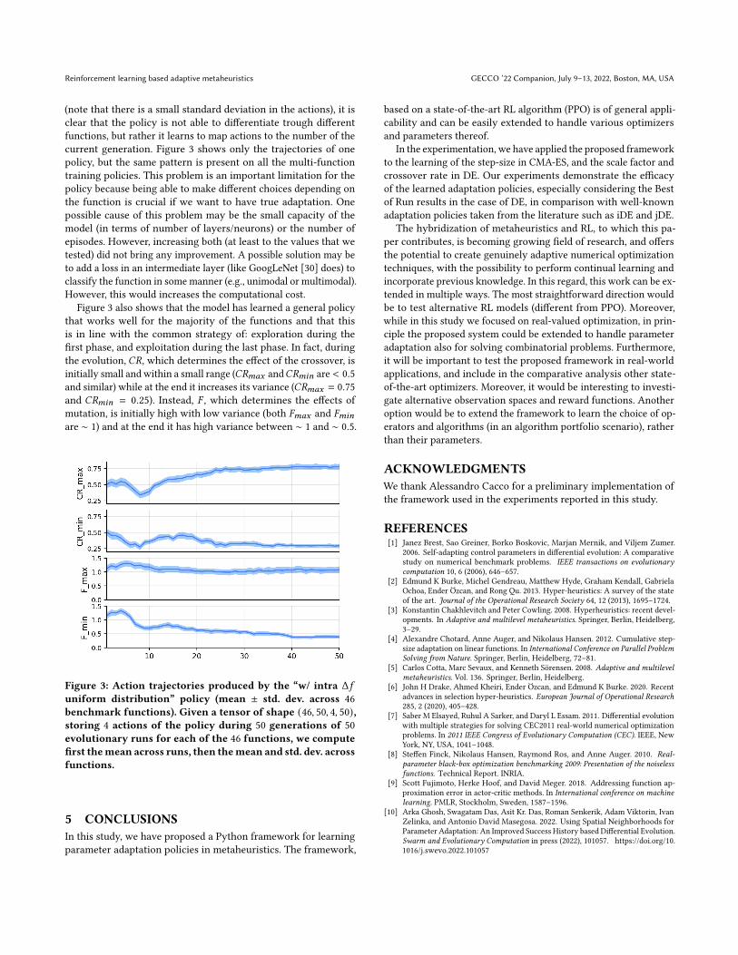
Another important observation can be made looking at Figure3. Because the trajectories are very similar across the functions

Reinforcement learning based adaptive metaheuristics GECCO ’22 Companion, July 9–13, 2022, Boston, MA, USA

(note that there is a small standard deviation in the actions), it isclear that the policy is not able to differentiate trough differentfunctions, but rather it learns to map actions to the number of thecurrent generation. Figure 3 shows only the trajectories of onepolicy, but the same pattern is present on all the multi-functiontraining policies. This problem is an important limitation for thepolicy because being able to make different choices depending onthe function is crucial if we want to have true adaptation. Onepossible cause of this problem may be the small capacity of themodel (in terms of number of layers/neurons) or the number ofepisodes. However, increasing both (at least to the values that wetested) did not bring any improvement. A possible solution may beto add a loss in an intermediate layer (like GoogLeNet [30] does) toclassify the function in somemanner (e.g., unimodal or multimodal).However, this would increases the computational cost.

Figure 3 also shows that the model has learned a general policythat works well for the majority of the functions and that thisis in line with the common strategy of: exploration during thefirst phase, and exploitation during the last phase. In fact, duringthe evolution, 𝐶𝑅, which determines the effect of the crossover, isinitially small and within a small range (𝐶𝑅𝑚𝑎𝑥 and𝐶𝑅𝑚𝑖𝑛 are < 0.5and similar) while at the end it increases its variance (𝐶𝑅𝑚𝑎𝑥 = 0.75and 𝐶𝑅𝑚𝑖𝑛 = 0.25). Instead, 𝐹 , which determines the effects ofmutation, is initially high with low variance (both 𝐹𝑚𝑎𝑥 and 𝐹𝑚𝑖𝑛

are ∼ 1) and at the end it has high variance between ∼ 1 and ∼ 0.5.

Figure 3: Action trajectories produced by the “w/ intra Δ𝑓uniform distribution” policy (mean ± std. dev. across 46benchmark functions). Given a tensor of shape (46, 50, 4, 50),storing 4 actions of the policy during 50 generations of 50evolutionary runs for each of the 46 functions, we computefirst themean across runs, then themean and std. dev. acrossfunctions.

5 CONCLUSIONSIn this study, we have proposed a Python framework for learningparameter adaptation policies in metaheuristics. The framework,

based on a state-of-the-art RL algorithm (PPO) is of general appli-cability and can be easily extended to handle various optimizersand parameters thereof.

In the experimentation, we have applied the proposed frameworkto the learning of the step-size in CMA-ES, and the scale factor andcrossover rate in DE. Our experiments demonstrate the efficacyof the learned adaptation policies, especially considering the Bestof Run results in the case of DE, in comparison with well-knownadaptation policies taken from the literature such as iDE and jDE.

The hybridization of metaheuristics and RL, to which this pa-per contributes, is becoming growing field of research, and offersthe potential to create genuinely adaptive numerical optimizationtechniques, with the possibility to perform continual learning andincorporate previous knowledge. In this regard, this work can be ex-tended in multiple ways. The most straightforward direction wouldbe to test alternative RL models (different from PPO). Moreover,while in this study we focused on real-valued optimization, in prin-ciple the proposed system could be extended to handle parameteradaptation also for solving combinatorial problems. Furthermore,it will be important to test the proposed framework in real-worldapplications, and include in the comparative analysis other state-of-the-art optimizers. Moreover, it would be interesting to investi-gate alternative observation spaces and reward functions. Anotheroption would be to extend the framework to learn the choice of op-erators and algorithms (in an algorithm portfolio scenario), ratherthan their parameters.

ACKNOWLEDGMENTSWe thank Alessandro Cacco for a preliminary implementation ofthe framework used in the experiments reported in this study.

REFERENCES[1] Janez Brest, Sao Greiner, Borko Boskovic, Marjan Mernik, and Viljem Zumer.

2006. Self-adapting control parameters in differential evolution: A comparativestudy on numerical benchmark problems. IEEE transactions on evolutionarycomputation 10, 6 (2006), 646–657.

[2] Edmund K Burke, Michel Gendreau, Matthew Hyde, Graham Kendall, GabrielaOchoa, Ender Özcan, and Rong Qu. 2013. Hyper-heuristics: A survey of the stateof the art. Journal of the Operational Research Society 64, 12 (2013), 1695–1724.

[3] Konstantin Chakhlevitch and Peter Cowling. 2008. Hyperheuristics: recent devel-opments. In Adaptive and multilevel metaheuristics. Springer, Berlin, Heidelberg,3–29.

[4] Alexandre Chotard, Anne Auger, and Nikolaus Hansen. 2012. Cumulative step-size adaptation on linear functions. In International Conference on Parallel ProblemSolving from Nature. Springer, Berlin, Heidelberg, 72–81.

[5] Carlos Cotta, Marc Sevaux, and Kenneth Sörensen. 2008. Adaptive and multilevelmetaheuristics. Vol. 136. Springer, Berlin, Heidelberg.

[6] John H Drake, Ahmed Kheiri, Ender Özcan, and Edmund K Burke. 2020. Recentadvances in selection hyper-heuristics. European Journal of Operational Research285, 2 (2020), 405–428.

[7] Saber M Elsayed, Ruhul A Sarker, and Daryl L Essam. 2011. Differential evolutionwith multiple strategies for solving CEC2011 real-world numerical optimizationproblems. In 2011 IEEE Congress of Evolutionary Computation (CEC). IEEE, NewYork, NY, USA, 1041–1048.

[8] Steffen Finck, Nikolaus Hansen, Raymond Ros, and Anne Auger. 2010. Real-parameter black-box optimization benchmarking 2009: Presentation of the noiselessfunctions. Technical Report. INRIA.

[9] Scott Fujimoto, Herke Hoof, and David Meger. 2018. Addressing function ap-proximation error in actor-critic methods. In International conference on machinelearning. PMLR, Stockholm, Sweden, 1587–1596.

[10] Arka Ghosh, Swagatam Das, Asit Kr. Das, Roman Senkerik, Adam Viktorin, IvanZelinka, and Antonio David Masegosa. 2022. Using Spatial Neighborhoods forParameter Adaptation: An Improved Success History based Differential Evolution.Swarm and Evolutionary Computation in press (2022), 101057. https://doi.org/10.1016/j.swevo.2022.101057

GECCO ’22 Companion, July 9–13, 2022, Boston, MA, USA Tessari and Iacca

[11] Nikolaus Hansen and Andreas Ostermeier. 2001. Completely derandomizedself-adaptation in evolution strategies. Evolutionary computation 9, 2 (2001),159–195.

[12] Zhenzhen Hu, Wenyin Gong, and Shuijia Li. 2021. Reinforcement learning-baseddifferential evolution for parameters extraction of photovoltaic models. EnergyReports 7 (2021), 916–928.

[13] Giovanni Iacca, Fabio Caraffini, and Ferrante Neri. 2015. Continuous ParameterPools in Ensemble Self-Adaptive Differential Evolution. In IEEE Symposium Serieson Computational Intelligence. IEEE, New York, NY, USA, 1529–1536.

[14] Giovanni Iacca, Ferrante Neri, Fabio Caraffini, and Ponnuthurai NagaratnamSuganthan. 2014. A differential evolution frameworkwith ensemble of parametersand strategies and pool of local search algorithms. In European conference on theapplications of evolutionary computation. Springer, Berlin, Heidelberg, 615–626.

[15] Kalyanmoy Deb Julian Blank. 2022. Parameter Tuning and Control: A Case Studyon Differential Evolution With Polynomial Mutation. https://www.egr.msu.edu/~kdeb/papers/c2022001.pdf

[16] Marcelo Gomes Pereira de LACERDA. 2021. Out-of-the-box parameter control forevolutionary and swarm-based algorithms with distributed reinforcement learning.Ph. D. Dissertation. Universidade Federal de Pernambuco.

[17] Sergey Levine and Vladlen Koltun. 2013. Guided policy search. In Internationalconference on machine learning. PMLR, Atlanta, GA, USA, 1–9.

[18] Wenwen Li, Ender Özcan, and Robert John. 2017. A learning automata-basedmultiobjective hyper-heuristic. IEEE Transactions on Evolutionary Computation23, 1 (2017), 59–73.

[19] Zhihui Li, Li Shi, Caitong Yue, Zhigang Shang, and Boyang Qu. 2019. Differen-tial evolution based on reinforcement learning with fitness ranking for solvingmultimodal multiobjective problems. Swarm and Evolutionary Computation 49(2019), 234–244.

[20] Manuel López-Ibáñez, Jérémie Dubois-Lacoste, Leslie Pérez Cáceres, Mauro Birat-tari, and Thomas Stützle. 2016. The irace package: Iterated racing for automaticalgorithm configuration. Operations Research Perspectives 3 (2016), 43–58.

[21] Alexander Nareyek. 2003. Choosing search heuristics by non-stationary re-inforcement learning. In Metaheuristics: Computer decision-making. Springer,Boston, MA, USA, 523–544.

[22] Karam M Sallam, Saber M Elsayed, Ripon K Chakrabortty, and Michael J Ryan.2020. Evolutionary framework with reinforcement learning-based mutationadaptation. IEEE Access 8 (2020), 194045–194071.

[23] Melissa Sánchez, Jorge M Cruz-Duarte, José carlos Ortíz-Bayliss, Hector Ceballos,Hugo Terashima-Marin, and Ivan Amaya. 2020. A systematic review of hyper-heuristics on combinatorial optimization problems. IEEE Access 8 (2020), 128068–128095.

[24] John Schulman, Filip Wolski, Prafulla Dhariwal, Alec Radford, and Oleg Klimov.2017. Proximal Policy Optimization Algorithms. arXiv:1707.06347.

[25] Gresa Shala, André Biedenkapp, Noor Awad, Steven Adriaensen, Marius Lindauer,and Frank Hutter. 2020. Learning step-size adaptation in CMA-ES. In InternationalConference on Parallel Problem Solving from Nature. Springer, Berlin, Heidelberg,691–706.

[26] Mudita Sharma, Alexandros Komninos, Manuel López-Ibáñez, and Dimitar Kaza-kov. 2019. Deep reinforcement learning based parameter control in differentialevolution. In Genetic and Evolutionary Computation Conference. ACM, New York,NY, USA, 709–717.

[27] Rainer Storn and Kenneth Price. 1997. Differential evolution–a simple andefficient heuristic for global optimization over continuous spaces. Journal ofglobal optimization 11, 4 (1997), 341–359.

[28] Jianyong Sun, Xin Liu, Thomas Bäck, and Zongben Xu. 2021. Learning adaptivedifferential evolution algorithm from optimization experiences by policy gradient.IEEE Transactions on Evolutionary Computation 25, 4 (2021), 666–680.

[29] Richard S Sutton and Andrew G Barto. 2018. Reinforcement learning: An intro-duction. MIT press, Cambridge, MA, USA.

[30] Christian Szegedy, Wei Liu, Yangqing Jia, Pierre Sermanet, Scott Reed, DragomirAnguelov, Dumitru Erhan, Vincent Vanhoucke, and Andrew Rabinovich. 2015.Going deeper with convolutions. In Conference on Computer Vision and Patternrecognition. IEEE, New York, NY, USA, 1–9.

[31] Ryoji Tanabe and Alex Fukunaga. 2013. Success-history based parameter adapta-tion for differential evolution. In Congress on Evolutionary Computation. IEEE,New York, NY, USA, 71–78.

[32] David H Wolpert and William G Macready. 1997. No free lunch theorems foroptimization. IEEE transactions on evolutionary computation 1, 1 (1997), 67–82.

[33] Anil Yaman, Giovanni Iacca, and Fabio Caraffini. 2019. A comparison of threedifferential evolution strategies in terms of early convergence with differentpopulation sizes. In AIP conference proceedings, Vol. 2070. AIP Publishing LLC,Melville, NY, USA, 020002.

[34] Anil Yaman, Giovanni Iacca, Matt Coler, George Fletcher, andMykola Pechenizkiy.2018. Multi-strategy differential evolution. In International Conference on theapplications of evolutionary computation. Springer, Berlin, Heidelberg, 617–633.