Sensors 2012, 12, 10990-11012; doi:10.3390/s120810990OPEN ACCESS

sensorsISSN 1424-8220

www.mdpi.com/journal/sensors

Article

A Comparison between Metaheuristics as Strategies forMinimizing Cyclic Instability in Ambient IntelligenceLeoncio A. Romero 1,?, Victor Zamudio 1,?, Rosario Baltazar 1, Efren Mezura 2, Marco Sotelo 1

and Vic Callaghan 3

1 Division of Research and Postgraduate Studies, Leon Institute of Technology, Leon, Guanajuato37290, Mexico; E-Mails: charobalmx@yahoo.com.mx (R.B.); masotelof@gmail.com (M.S.)

2 Laboratorio Nacional de Informatica Avanzada, Xalapa, Veracruz 91000, Mexico;E-Mail: emezura@lania.mx

3 School of Computer Science and Electronic Engineering, University of Essex,Wivenhoe Park CO4 3SQ, UK; E-Mail: vic@essex.ac.uk

? Authors to whom correspondence should be addressed; E-Mails: leoncior@acm.org (L.A.R.);vic.zamudio@ieee.org (V.Z.).

Received: 3 June 2012; in revised form: 3 July 2012 / Accepted: 10 July 2012 /Published: 8 August 2012

Abstract: In this paper we present a comparison between six novel approaches to thefundamental problem of cyclic instability in Ambient Intelligence. These approaches arebased on different optimization algorithms, Particle Swarm Optimization (PSO), Bee SwarmOptimization (BSO), micro Particle Swarm Optimization (µ-PSO), Artificial ImmuneSystem (AIS), Genetic Algorithm (GA) and Mutual Information Maximization for InputClustering (MIMIC). In order to be able to use these algorithms, we introduced the concept ofAverage Cumulative Oscillation (ACO), which enabled us to measure the average behavior ofthe system. This approach has the advantage that it does not need to analyze the topologicalproperties of the system, in particular the loops, which can be computationally expensive.In order to test these algorithms we used the well-known discrete system called the Gameof Life for 9, 25, 49 and 289 agents. It was found that PSO and µ-PSO have the bestperformance in terms of the number of agents locked. These results were confirmed usingthe Wilcoxon Signed Rank Test. This novel and successful approach is very promising andcan be used to remove instabilities in real scenarios with a large number of agents (includingnomadic agents) and complex interactions and dependencies among them.

Sensors 2012, 12 10991

Keywords: cyclic instability; ambient intelligence; locking

1. Introduction

Any computer system can have errors and Ambient Intelligence is not exempt from them. Cyclicalinstability is a fundamental problem characterized by the presence of unexpected oscillations caused bythe interaction of the rules governing the agents involved [1–4].

The problem of cyclical instability in Ambient Intelligence is a problem that has received littleattention by the designers of intelligent environments [2,5]. However in order to achieve the visionof AmI this problem must be solved.

In the literature there are several strategies reported based on analyzing the connectivity among theagents due to their rules. The first one the Instability Prevention System INPRES is based on analyzingthe topological properties of the Interaction Network. The Interaction Network is the digraph associatedto the system and captures the dependencies of the rules between agents. INPRES finds the loops andlocks a subset of agents on a loop, preventing them to change their state [1–4]. INPRES has been testedsuccessfully in system with low density of interconnections and static rules (nomadic devices and timevariant rules are not allowed). However when the number of agents involved in the system increases (withhigh dependencies among them) or when the agents are nomadic, the approach suggested by INPRES isnot practical, due to the computational cost.

Additionally Action Selection Algorithms map the relationship between agents, rules and selectionalgorithms, into a simple linear system [6]. However this approach has not been tested in real orsimulated scenarios nor nomadic agents.

The approach presented in this paper translates the problem of cyclic instability into a problem ofintelligent optimization, moving from exhaustive search techniques to metaheuristics searching.

In this paper we compare the results of Particle Swarm Optimization (PSO), Bee Swarm Optimization(BSO), micro Particle Swarm Optimization (µ-PSO), Artificial Immune System (AIS), Genetic Algorithm(GA) and Mutual Information Maximization for Input Clustering (MIMIC) when applied to the problemof cyclic instability. These algorithms find a good set of agents to be locked, in order to minimize theoscillatory behavior of the system. This approach has the advantage that there is no need to analyze thedependencies of the rules of the agents (as in the case of INPRES). We used the game of life [7] to testthis approach, where each cell represents an agent of the system.

2. Cyclic Instability in Intelligent Environments

The scenarios of intelligent environments are governed by a set of rules, which are directly involved inthe unstable behavior, and can lead the system to multiple changes over a period of time. These changescan cause interference with other devices, or unwanted behavior [1–4].

The state of a system s(t) is defined as the logarithm base 10 of the binary vectors of the agents.A turned-on agent was represented with 1 while a shut-down agent will be represented with 0. Therepresentation of the state of the system is shown in Equation (1):

Sensors 2012, 12 10992

s(t) = log(s) (1)

where s(t) is the state of the system at time t, and s is base-10 representation of the binary number ofthe state of the system.

3. Optimization Algorithms

3.1. Particle Swarm Optimization

The Particle Swarm Optimization (PSO) algorithm was proposed by Kennedy and Everhart [8,9]. It isbased on the choreography of a flock of birds [8–13], wing a social metaphor [14] where each individualbrings their knowledge to get a better solution. There are three factors that influence the change of theparticle state or behavior:

• Knowledge of the environment or adaptation is the importance given to past experiences.• Experience or local memory is the local importance given to best result found.• The experience of its neighbors or neighborhood memory is the importance given to the best result

achieved by their neighbors.

The basic PSO algorithm [9] uses two equations. Equation (2), which is used to find the velocity,describes the size and direction of the step that will be taken by the particles and is based on theknowledge achieved until that moment.

vi = wvi + c1r1 (lBesti − xi) + c2r2 (gBest− xi) (2)

where:vi is the velocity of the i-th particle, i = 1, 2 . . . , N ,N is the number of the population,w is the environment adjustment factor ,c1 is the memory factor of neighborhood ,c2 is memory factor ,r1 and r2 are random numbers in range [0, 1] ,lBest is the best local particle founded for the i-th particle ,gBest is the best general particle founded until that moment for all particles.

Equation (3) updates the current position of the particle to the new position using the result of thevelocity equation.

xi = xi + vi (3)

where xi is the position of the i-th particle.The PSO algorithm [9] is shown in the Algorithm 1:

Sensors 2012, 12 10993

Algorithm 1 PSO Algorithm.Data: P ∈ [3, 6] (number of particles), c1 ∈ R, c2 ∈ R, w ∈ [0, 1] , G (maximum allowed functionevaluations).Result: GBest (best solution found)

1. Initialize particles ’ position and velocity randomly;2. For g = 1 to G do

(a) Recalculate best particles position gBest(b) Select the local best position lBest(c) For each Xig, i = 1, . . . , P do

i. Recalculate particle speedii. Recalculate particle position

3.2. Binary PSO

Binary PSO [13,14] was designed to work in binary spaces. Binary PSO select the lBest and gBestparticles in the same way as PSO. The main difference between binary PSO and normal PSO are theequations that are used to update the particle velocity and position. The equation for updating thevelocity is based on probabilities but these probabilities must be in the range [0, 1]. A mapping isestablished for all real values of velocity to the range [0, 1]. The normalization Equation (4) used here isa sigmoid function.

vij (t) = sigmoid (vij (t)) =1

1 + e−vij(t)(4)

and Equation (5) is used to update the new particle position.

xij (t+ 1) =

{1 if rij < sigmoid (vij (t+ 1))

0 in other case(5)

where rij is a random vector with uniform values in the range [0, 1].

3.3. Micro PSO

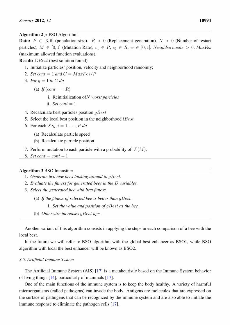
µ-PSO algorithm [15,16] is a modification made to the original PSO algorithm in order to work withsmall populations (See Algorithm 2). This algorithm use replacement and mutation to be included in theoriginal PSO algorithm, and allow to the algorithm avoid local optima.

3.4. Bee Swarm Optimization

BSO algorithm [14] is based on PSO and Bee algorithm (See Algorithm 3). It uses a local searchalgorithm to intensify the search. This algorithm was proposed by Sotelo [14], where the changes madeto PSO allowed finding a new best Global in the current population.

Sensors 2012, 12 10994

Algorithm 2 µ-PSO Algorithm.Data: P ∈ [3, 6] (population size). R > 0 (Replacement generation), N > 0 (Number of restartparticles), M ∈ [0, 1] (Mutation Rate), c1 ∈ R, c2 ∈ R, w ∈ [0, 1], Neighborhoods > 0, MaxFes(maximum allowed function evaluations).Result: GBest (best solution found)

1. Initialize particles’ position, velocity and neighborhood randomly;2. Set cont = 1 and G =MaxFes/P

3. For g = 1 to G do

(a) If (cont == R)

i. Reinitialization ofN worst particlesii. Set cont = 1

4. Recalculate best particles position gBest5. Select the local best position in the neighborhood lBest6. For each Xig, i = 1, . . . , P do

(a) Recalculate particle speed(b) Recalculate particle position

7. Perform mutation to each particle with a probability of P (M);8. Set cont = cont+ 1

Algorithm 3 BSO Intensifier.1. Generate two new bees looking around to gBest.2. Evaluate the fitness for generated bees in the D variables.3. Select the generated bee with best fitness.

(a) If the fitness of selected bee is better than gBest

i. Set the value and position of gBest as the bee.

(b) Otherwise increases gBest age.

Another variant of this algorithm consists in applying the steps in each comparison of a bee with thelocal best.

In the future we will refer to BSO algorithm with the global best enhancer as BSO1, while BSOalgorithm with local the best enhancer will be known as BSO2.

3.5. Artificial Immune System

The Artificial Immune System (AIS) [17] is a metaheuristic based on the Immune System behaviorof living things [14], particularly of mammals [17].

One of the main functions of the immune system is to keep the body healthy. A variety of harmfulmicroorganisms (called pathogens) can invade the body. Antigens are molecules that are expressed onthe surface of pathogens that can be recognized by the immune system and are also able to initiate theimmune response to eliminate the pathogen cells [17].

Sensors 2012, 12 10995

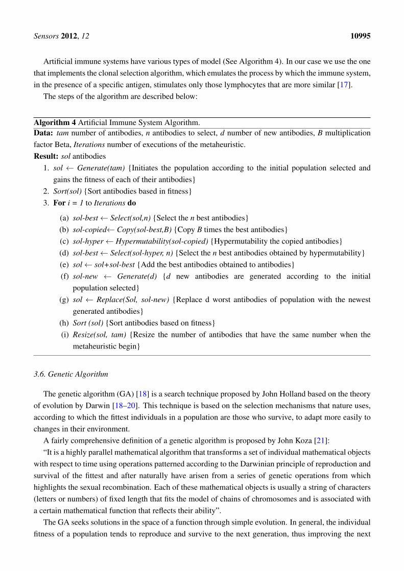
Artificial immune systems have various types of model (See Algorithm 4). In our case we use the onethat implements the clonal selection algorithm, which emulates the process by which the immune system,in the presence of a specific antigen, stimulates only those lymphocytes that are more similar [17].

The steps of the algorithm are described below:

Algorithm 4 Artificial Immune System Algorithm.Data: tam number of antibodies, n antibodies to select, d number of new antibodies, B multiplicationfactor Beta, Iterations number of executions of the metaheuristic.Result: sol antibodies

1. sol ← Generate(tam) {Initiates the population according to the initial population selected andgains the fitness of each of their antibodies}

2. Sort(sol) {Sort antibodies based in fitness}3. For i = 1 to Iterations do

(a) sol-best← Select(sol,n) {Select the n best antibodies}(b) sol-copied← Copy(sol-best,B) {Copy B times the best antibodies}(c) sol-hyper← Hypermutability(sol-copied) {Hypermutability the copied antibodies}(d) sol-best← Select(sol-hyper, n) {Select the n best antibodies obtained by hypermutability}(e) sol← sol+sol-best {Add the best antibodies obtained to antibodies}(f) sol-new ← Generate(d) {d new antibodies are generated according to the initial

population selected}(g) sol ← Replace(Sol, sol-new) {Replace d worst antibodies of population with the newest

generated antibodies}(h) Sort (sol) {Sort antibodies based on fitness}(i) Resize(sol, tam) {Resize the number of antibodies that have the same number when the

metaheuristic begin}

3.6. Genetic Algorithm

The genetic algorithm (GA) [18] is a search technique proposed by John Holland based on the theoryof evolution by Darwin [18–20]. This technique is based on the selection mechanisms that nature uses,according to which the fittest individuals in a population are those who survive, to adapt more easily tochanges in their environment.

A fairly comprehensive definition of a genetic algorithm is proposed by John Koza [21]:“It is a highly parallel mathematical algorithm that transforms a set of individual mathematical objects

with respect to time using operations patterned according to the Darwinian principle of reproduction andsurvival of the fittest and after naturally have arisen from a series of genetic operations from whichhighlights the sexual recombination. Each of these mathematical objects is usually a string of characters(letters or numbers) of fixed length that fits the model of chains of chromosomes and is associated witha certain mathematical function that reflects their ability”.

The GA seeks solutions in the space of a function through simple evolution. In general, the individualfitness of a population tends to reproduce and survive to the next generation, thus improving the next

Sensors 2012, 12 10996

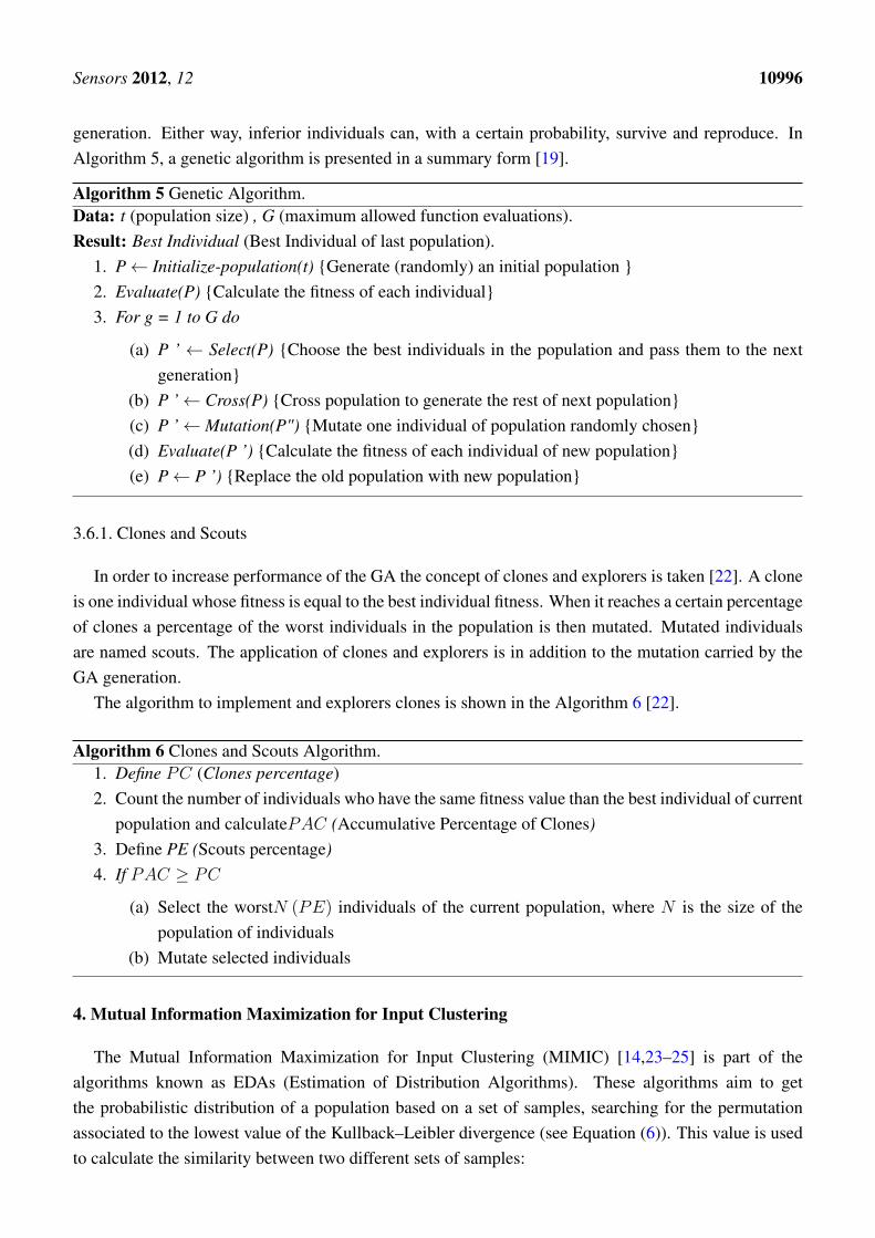
generation. Either way, inferior individuals can, with a certain probability, survive and reproduce. InAlgorithm 5, a genetic algorithm is presented in a summary form [19].

Algorithm 5 Genetic Algorithm.Data: t (population size) , G (maximum allowed function evaluations).Result: Best Individual (Best Individual of last population).

1. P← Initialize-population(t) {Generate (randomly) an initial population }2. Evaluate(P) {Calculate the fitness of each individual}3. For g = 1 to G do

(a) P ’ ← Select(P) {Choose the best individuals in the population and pass them to the nextgeneration}

(b) P ’← Cross(P) {Cross population to generate the rest of next population}(c) P ’← Mutation(P") {Mutate one individual of population randomly chosen}(d) Evaluate(P ’) {Calculate the fitness of each individual of new population}(e) P← P ’) {Replace the old population with new population}

3.6.1. Clones and Scouts

In order to increase performance of the GA the concept of clones and explorers is taken [22]. A cloneis one individual whose fitness is equal to the best individual fitness. When it reaches a certain percentageof clones a percentage of the worst individuals in the population is then mutated. Mutated individualsare named scouts. The application of clones and explorers is in addition to the mutation carried by theGA generation.

The algorithm to implement and explorers clones is shown in the Algorithm 6 [22].

Algorithm 6 Clones and Scouts Algorithm.1. Define PC (Clones percentage)2. Count the number of individuals who have the same fitness value than the best individual of current

population and calculatePAC (Accumulative Percentage of Clones)3. Define PE (Scouts percentage)4. If PAC ≥ PC

(a) Select the worstN (PE) individuals of the current population, where N is the size of thepopulation of individuals

(b) Mutate selected individuals

4. Mutual Information Maximization for Input Clustering

The Mutual Information Maximization for Input Clustering (MIMIC) [14,23–25] is part of thealgorithms known as EDAs (Estimation of Distribution Algorithms). These algorithms aim to getthe probabilistic distribution of a population based on a set of samples, searching for the permutationassociated to the lowest value of the Kullback–Leibler divergence (see Equation (6)). This value is usedto calculate the similarity between two different sets of samples:

Sensors 2012, 12 10997

Hπl = hl (Xin) +

n−1∑j=1

hl (xij|xij+1) (6)

where:h (X) = −

∑x p (X = x) log p (X = x) is Shannon’s entropy of X variable

h (X|Y ) = −∑

x p (X|Y ) log p (Y = y), whereh (X|Y = y) = −

∑X p (X = x|Y = y) log (X = x|Y = y), is the X entropy given Y .

This algorithm suppose that the different variables have a bivariate dependency described byEquation (7).

pπl (x) = pl (xi1|xi2) � pl (xi2|xi3) · . . . pl (xin−1|xin) pl (xin) (7)

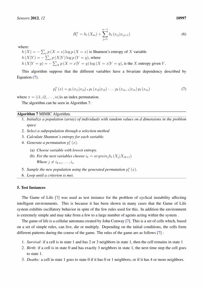
where π = (i1, i2, . . . , in)is an index permutation.The algorithm can be seen in Algorithm 7:

Algorithm 7 MIMIC Algorithm.1. Initialize a population (array) of individuals with random values on d dimensions in the problem

space2. Select a subpopulation through a selection method3. Calculate Shannon’s entropy for each variable.4. Generate a permutation pπl (x).

(a) Choose variable with lowest entropy.(b) For the next variables choose ik = argminjhl (Xj|Xik+1)

Where j 6= ik+i, . . . , in

5. Sample the new population using the generated permutation pπl (x).6. Loop until a criterion is met.

5. Test Instances

The Game of Life [7] was used as test instance for the problem of cyclical instability affectingintelligent environments. This is because it has been shown in many cases that the Game of Lifesystem exhibits oscillatory behavior in spite of the few rules used for this. In addition the environmentis extremely simple and may take from a few to a large number of agents acting within the system .

The game of life is a cellular automata created by John Conway [7]. This is a set of cells which, basedon a set of simple rules, can live, die or multiply. Depending on the initial conditions, the cells formdifferent patterns during the course of the game. The rules of the game are as follows [7] :

1. Survival: if a cell is in state 1 and has 2 or 3 neighbors in state 1, then the cell remains in state 12. Birth: if a cell is in state 0 and has exactly 3 neighbors in state 1, the next time step the cell goes

to state 1.3. Deaths: a cell in state 1 goes to state 0 if it has 0 or 1 neighbors, or if it has 4 or more neighbors.

Sensors 2012, 12 10998

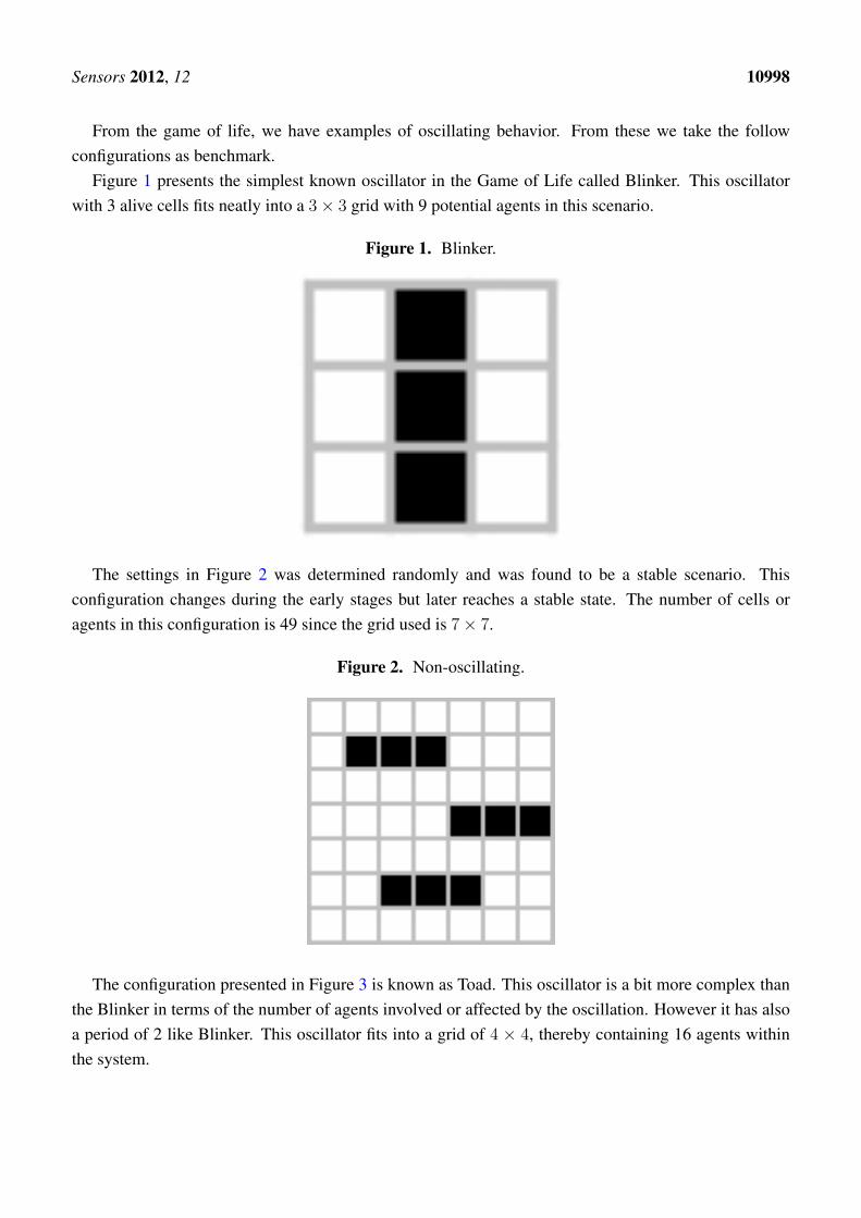
From the game of life, we have examples of oscillating behavior. From these we take the followconfigurations as benchmark.

Figure 1 presents the simplest known oscillator in the Game of Life called Blinker. This oscillatorwith 3 alive cells fits neatly into a 3× 3 grid with 9 potential agents in this scenario.

Figure 1. Blinker.

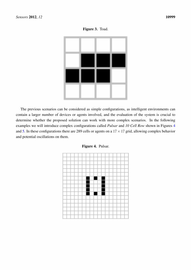
The settings in Figure 2 was determined randomly and was found to be a stable scenario. Thisconfiguration changes during the early stages but later reaches a stable state. The number of cells oragents in this configuration is 49 since the grid used is 7× 7.

Figure 2. Non-oscillating.

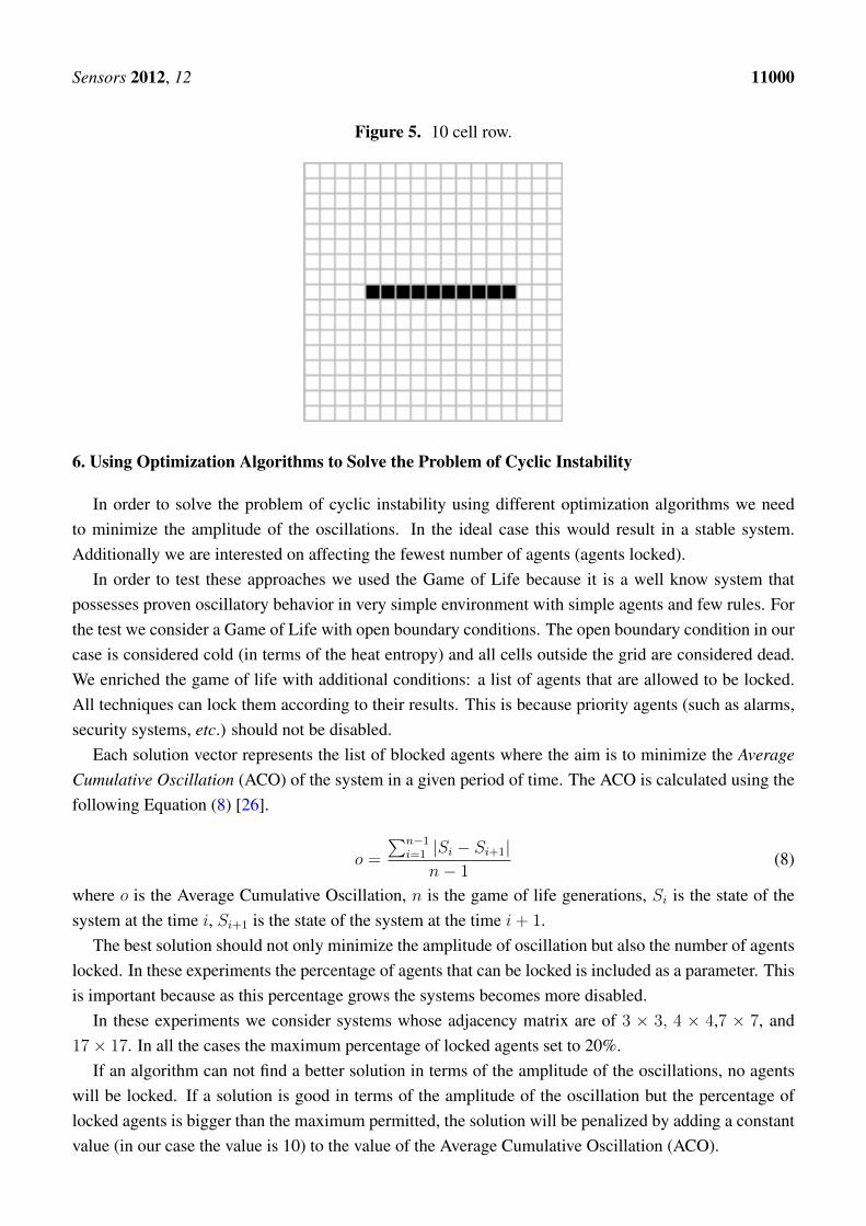
The configuration presented in Figure 3 is known as Toad. This oscillator is a bit more complex thanthe Blinker in terms of the number of agents involved or affected by the oscillation. However it has alsoa period of 2 like Blinker. This oscillator fits into a grid of 4 × 4, thereby containing 16 agents withinthe system.

Sensors 2012, 12 10999

Figure 3. Toad.

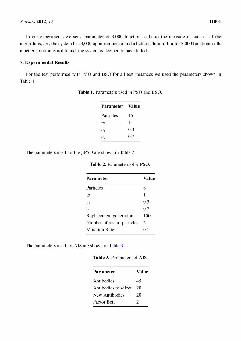
The previous scenarios can be considered as simple configurations, as intelligent environments cancontain a larger number of devices or agents involved, and the evaluation of the system is crucial todetermine whether the proposed solution can work with more complex scenarios. In the followingexamples we will introduce complex configurations called Pulsar and 10 Cell Row shown in Figures 4and 5. In these configurations there are 289 cells or agents on a 17× 17 grid, allowing complex behaviorand potential oscillations on them.

Figure 4. Pulsar.

Sensors 2012, 12 11000

Figure 5. 10 cell row.

6. Using Optimization Algorithms to Solve the Problem of Cyclic Instability

In order to solve the problem of cyclic instability using different optimization algorithms we needto minimize the amplitude of the oscillations. In the ideal case this would result in a stable system.Additionally we are interested on affecting the fewest number of agents (agents locked).

In order to test these approaches we used the Game of Life because it is a well know system thatpossesses proven oscillatory behavior in very simple environment with simple agents and few rules. Forthe test we consider a Game of Life with open boundary conditions. The open boundary condition in ourcase is considered cold (in terms of the heat entropy) and all cells outside the grid are considered dead.We enriched the game of life with additional conditions: a list of agents that are allowed to be locked.All techniques can lock them according to their results. This is because priority agents (such as alarms,security systems, etc.) should not be disabled.

Each solution vector represents the list of blocked agents where the aim is to minimize the AverageCumulative Oscillation (ACO) of the system in a given period of time. The ACO is calculated using thefollowing Equation (8) [26].

o =

∑n−1i=1 |Si − Si+1|

n− 1(8)

where o is the Average Cumulative Oscillation, n is the game of life generations, Si is the state of thesystem at the time i, Si+1 is the state of the system at the time i+ 1.

The best solution should not only minimize the amplitude of oscillation but also the number of agentslocked. In these experiments the percentage of agents that can be locked is included as a parameter. Thisis important because as this percentage grows the systems becomes more disabled.

In these experiments we consider systems whose adjacency matrix are of 3 × 3, 4 × 4,7 × 7, and17× 17. In all the cases the maximum percentage of locked agents set to 20%.

If an algorithm can not find a better solution in terms of the amplitude of the oscillations, no agentswill be locked. If a solution is good in terms of the amplitude of the oscillation but the percentage oflocked agents is bigger than the maximum permitted, the solution will be penalized by adding a constantvalue (in our case the value is 10) to the value of the Average Cumulative Oscillation (ACO).

Sensors 2012, 12 11001

In our experiments we set a parameter of 3,000 functions calls as the measure of success of thealgorithms, i.e., the system has 3,000 opportunities to find a better solution. If after 3,000 functions callsa better solution is not found, the system is deemed to have failed.

7. Experimental Results

For the test performed with PSO and BSO for all test instances we used the parameters shown inTable 1.

Table 1. Parameters used in PSO and BSO.

Parameter Value

Particles 45w 1c1 0.3c2 0.7

The parameters used for the µPSO are shown in Table 2.

Table 2. Parameters of µ-PSO.

Parameter Value

Particles 6w 1c1 0.3c2 0.7Replacement generation 100Number of restart particles 2Mutation Rate 0.1

The parameters used for AIS are shown in Table 3.

Table 3. Parameters of AIS.

Parameter Value

Antibodies 45Antibodies to select 20New Antibodies 20Factor Beta 2

Sensors 2012, 12 11002

The parameters used for GA are shown in Table 4.

Table 4. Parameters of GA.

Parameter Value

Chromosomes 45Mutation percentage 0.15Elitism 0.2Clones percentage 0.3Scouts percentage 0.8

For the test performed with MIMIC for all test instances we used the parameters shown in Table 5.

Table 5. Parameters used in MIMIC.

Parameter Value

Individuals 100Elitism 0.5

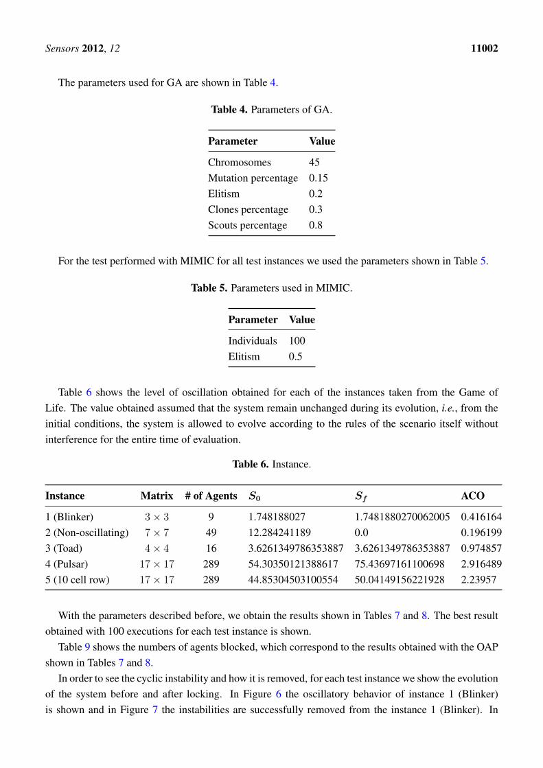
Table 6 shows the level of oscillation obtained for each of the instances taken from the Game ofLife. The value obtained assumed that the system remain unchanged during its evolution, i.e., from theinitial conditions, the system is allowed to evolve according to the rules of the scenario itself withoutinterference for the entire time of evaluation.

Table 6. Instance.

Instance Matrix # of Agents S0 Sf ACO

1 (Blinker) 3× 3 9 1.748188027 1.7481880270062005 0.4161642 (Non-oscillating) 7× 7 49 12.284241189 0.0 0.1961993 (Toad) 4× 4 16 3.6261349786353887 3.6261349786353887 0.9748574 (Pulsar) 17× 17 289 54.30350121388617 75.43697161100698 2.9164895 (10 cell row) 17× 17 289 44.85304503100554 50.04149156221928 2.23957

With the parameters described before, we obtain the results shown in Tables 7 and 8. The best resultobtained with 100 executions for each test instance is shown.

Table 9 shows the numbers of agents blocked, which correspond to the results obtained with the OAPshown in Tables 7 and 8.

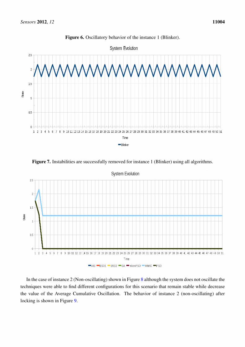
In order to see the cyclic instability and how it is removed, for each test instance we show the evolutionof the system before and after locking. In Figure 6 the oscillatory behavior of instance 1 (Blinker)is shown and in Figure 7 the instabilities are successfully removed from the instance 1 (Blinker). In

Sensors 2012, 12 11003

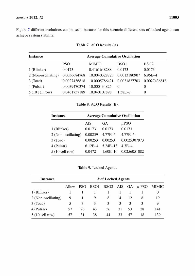
Figure 7 different evolutions can be seen, because for this scenario different sets of locked agents canachieve system stability.

Table 7. ACO Results (A).

Instance Average Cumulative Oscillation

PSO MIMIC BSO1 BSO21 (Blinker) 0.0173 0.4161648288 0.0173 0.01732 (Non-oscillating) 0.0036684768 10.0040328723 0.0013180907 6.96E–43 (Toad) 0.0027436818 10.0005786421 0.0031827703 0.00274368184 (Pulsar) 0.0039470374 10.000434825 0 05 (10 cell row) 0.0461757189 10.040107898 1.58E–7 0

Table 8. ACO Results (B).

Instance Average Cumulative Oscillation

AIS GA µPSO1 (Blinker) 0.0173 0.0173 0.01732 (Non-oscillating) 0.00239 4.77E–6 4.77E–63 (Toad) 0.00253 0.00253 0.00253079734 (Pulsar) 6.12E–4 5.24E–13 4.3E–45 (10 cell row) 0.0472 1.60E–10 0.0256051082

Table 9. Locked Agents.

Instance # of Locked Agents

Allow PSO BSO1 BSO2 AIS GA µ-PSO MIMIC1 (Blinker) 1 1 1 1 1 1 1 02 (Non-oscillating) 9 1 9 8 4 12 8 193 (Toad) 5 3 3 3 3 3 3 94 (Pulsar) 57 26 43 56 31 53 28 1415 (10 cell row) 57 31 38 44 33 57 18 139

Sensors 2012, 12 11004

Figure 6. Oscillatory behavior of the instance 1 (Blinker).

Figure 7. Instabilities are successfully removed for instance 1 (Blinker) using all algorithms.

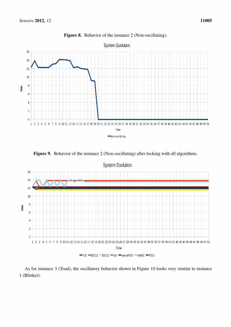
In the case of instance 2 (Non-oscillating) shown in Figure 8 although the system does not oscillate thetechniques were able to find different configurations for this scenario that remain stable while decreasethe value of the Average Cumulative Oscillation. The behavior of instance 2 (non-oscillating) afterlocking is shown in Figure 9.

Sensors 2012, 12 11005

Figure 8. Behavior of the instance 2 (Non-oscillating).

Figure 9. Behavior of the instance 2 (Non-oscillating) after locking with all algorithms.

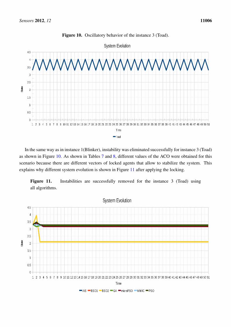
As for instance 3 (Toad), the oscillatory behavior shown in Figure 10 looks very similar to instance1 (Blinker).

Sensors 2012, 12 11006

Figure 10. Oscillatory behavior of the instance 3 (Toad).

In the same way as in instance 1(Blinker), instability was eliminated successfully for instance 3 (Toad)as shown in Figure 10. As shown in Tables 7 and 8, different values of the ACO were obtained for thisscenario because there are different vectors of locked agents that allow to stabilize the system. Thisexplains why different system evolution is shown in Figure 11 after applying the locking.

Figure 11. Instabilities are successfully removed for the instance 3 (Toad) usingall algorithms.

Sensors 2012, 12 11007

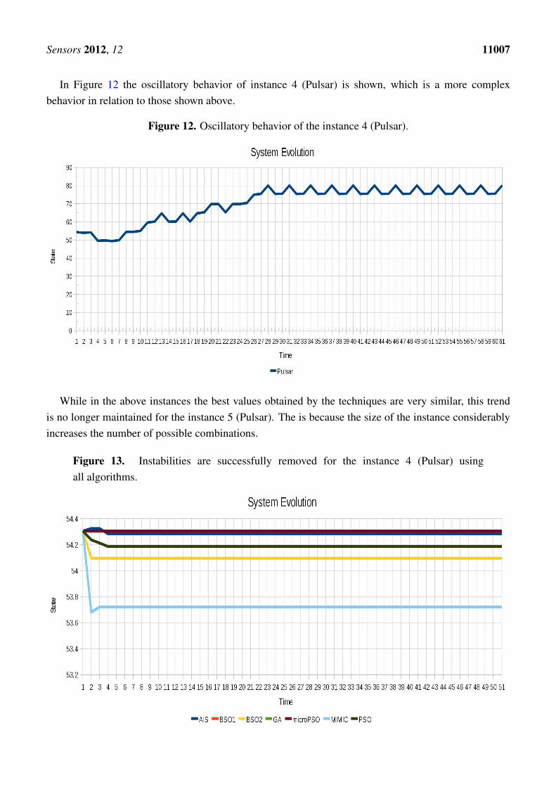
In Figure 12 the oscillatory behavior of instance 4 (Pulsar) is shown, which is a more complexbehavior in relation to those shown above.

Figure 12. Oscillatory behavior of the instance 4 (Pulsar).

While in the above instances the best values obtained by the techniques are very similar, this trendis no longer maintained for the instance 5 (Pulsar). The is because the size of the instance considerablyincreases the number of possible combinations.

Figure 13. Instabilities are successfully removed for the instance 4 (Pulsar) usingall algorithms.

Sensors 2012, 12 11008

Most importantly, despite the difference in the results between the various techniques, it was possibleto stabilize the system with different combinations of locked agents, showing that depending on thescenario there may be more than one set of locked agents with which the system can become stable. Thisis showcased by the different results obtained for the instance 4 (Pulsar) in the level of instability (referto Figure 13), where we can see how quickly the system stabilizes in each of the different configurationsachieved by the optimization techniques.

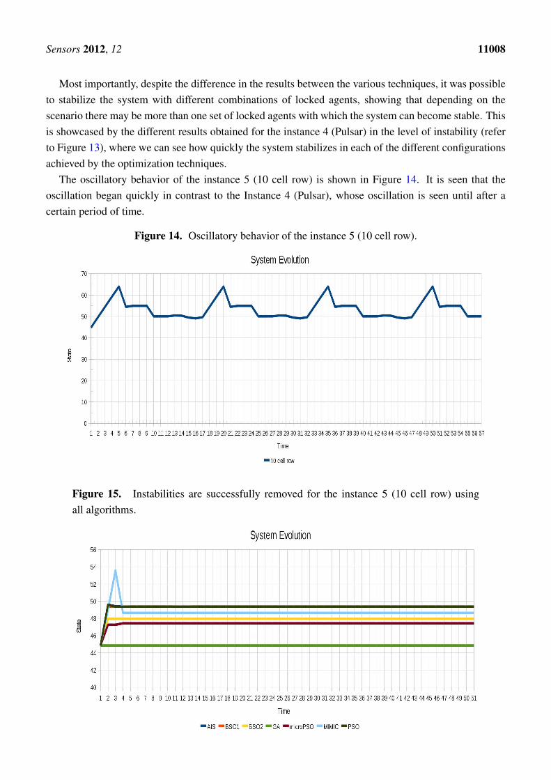
The oscillatory behavior of the instance 5 (10 cell row) is shown in Figure 14. It is seen that theoscillation began quickly in contrast to the Instance 4 (Pulsar), whose oscillation is seen until after acertain period of time.

Figure 14. Oscillatory behavior of the instance 5 (10 cell row).

Figure 15. Instabilities are successfully removed for the instance 5 (10 cell row) usingall algorithms.

Sensors 2012, 12 11009

For the instance 5 (10 cell row), again the number of agents represented is therefore significant. Theperformance results are similar to those described for instance 4 (Toad) and the best results obtained bythe techniques vary with respect to each other. The behavior without oscillation is shown in Figure 15.The difference between the behavior of each algorithm responds to the different sets of locked agents byeach of the techniques.

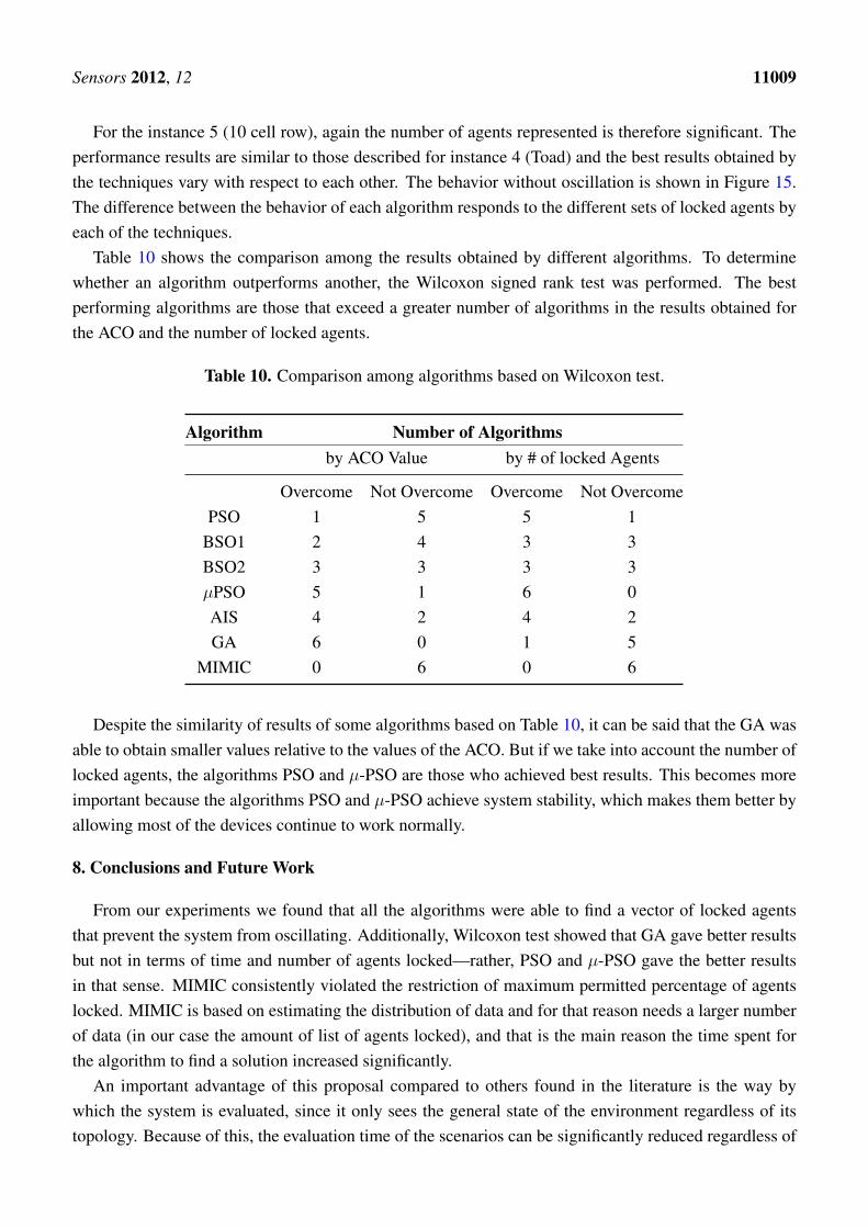
Table 10 shows the comparison among the results obtained by different algorithms. To determinewhether an algorithm outperforms another, the Wilcoxon signed rank test was performed. The bestperforming algorithms are those that exceed a greater number of algorithms in the results obtained forthe ACO and the number of locked agents.

Table 10. Comparison among algorithms based on Wilcoxon test.

Algorithm Number of Algorithmsby ACO Value by # of locked Agents

Overcome Not Overcome Overcome Not OvercomePSO 1 5 5 1

BSO1 2 4 3 3BSO2 3 3 3 3µPSO 5 1 6 0AIS 4 2 4 2GA 6 0 1 5

MIMIC 0 6 0 6

Despite the similarity of results of some algorithms based on Table 10, it can be said that the GA wasable to obtain smaller values relative to the values of the ACO. But if we take into account the number oflocked agents, the algorithms PSO and µ-PSO are those who achieved best results. This becomes moreimportant because the algorithms PSO and µ-PSO achieve system stability, which makes them better byallowing most of the devices continue to work normally.

8. Conclusions and Future Work

From our experiments we found that all the algorithms were able to find a vector of locked agentsthat prevent the system from oscillating. Additionally, Wilcoxon test showed that GA gave better resultsbut not in terms of time and number of agents locked—rather, PSO and µ-PSO gave the better resultsin that sense. MIMIC consistently violated the restriction of maximum permitted percentage of agentslocked. MIMIC is based on estimating the distribution of data and for that reason needs a larger numberof data (in our case the amount of list of agents locked), and that is the main reason the time spent forthe algorithm to find a solution increased significantly.

An important advantage of this proposal compared to others found in the literature is the way bywhich the system is evaluated, since it only sees the general state of the environment regardless of itstopology. Because of this, the evaluation time of the scenarios can be significantly reduced regardless of

Sensors 2012, 12 11010

the number of agents that form part of the system. Additionally, the possibility of a proposal able to workwith any scenario can be more clearly distinguished in real time, which helps to improve their operation.

This approach based on the concept of Average Cumulative Oscillation opens the possibility forother algorithms to be applied to the problem of cyclic instability, in general algorithms for discreteoptimization. In particular we are interested in testing this approach for the case of nomadic and weightedagents and with different percentage of locked agents. Also it is possible to improve the estimation of theoscillation in order to discriminate between stable systems with abrupt changes and systems with smalloscillations, because in some cases it is possible to get small values of Average Cumulative Oscillationin oscillating systems. We hope to report these results in future.

Acknowledgments

The authors want to thank Jorge Soria for their comments and suggestions to his work.Leoncio Romero acknowledges the support of the National Council for Science and TechnologyCONACyT. Additionally, E. Mezura acknowledges the support from CONACyT through projectNo. 79809.

References

1. Zamudio, V.M. Understanding and Preventing Periodic Behavior in Ambient Intelligence. Ph.D.Thesis, University of Essex, Southend-on-Sea, UK, 2008.

2. Zamudio, V.; Callaghan, V. Facilitating the ambient intelligent vision: A theorem, representationand solution for instability in rule-based multi-agent systems. Int. Trans. Syst. Sci. Appl. 2008, 4,108–121.

3. Zamudio, V.; Callaghan, V. Understanding and avoiding interaction based instability in pervasivecomputing environments. Int. J. Pervasive Comput. Commun. 2009, 5, 163–186.

4. Zamudio, V.; Baltazar, R.; Casillas, M. c-INPRES: Coupling analysis towards locking optimizationin ambient intelligence. In Proceedings of the 6th International Conference on IntelligentEnvironments IE10, Monash University (Sunway campus), Kuala Lumpur, Malaysia, July 2010.

5. Egerton, A.; Zamudio, V.; Callaghan, V.; Clarke, G. Instability and Irrationality: Destructive andConstructive Services within Intelligent Environments; Essex University: Southend-on-Sea, UK,2009.

6. Gaber, J. Action selection algorithms for autonomous system in pervasive environment:A computational approach. ACM Trans. Auton. Adapt. Syst. 2011, doi:1921641.1921651.

7. Nápoles, J.E. El juego de la Vida: Geometría Dinámica. M.S. Thesis, Universidad de la Cuencadel Plata, Corrientes, Argentina.

8. Carlise, A.; Dozier, G. An off-the-shelf PSO. In Proceedings of the Particle Swarm OptimizationWorkshop, Indianapolis, IN, USA, April 2001.

9. Eberhart, R.C.; Shi, Y. Particle swarm optimization: Developments, applications and resources. InProceedings of the Evolutionary Computation, Seoul, Korean, May 2001; pp. 82–86.

Sensors 2012, 12 11011

10. Coello, C.A.; Salazar, M. MOPSO: A proposal for multiple Objetive Particle Swarm Optimization.In Proceedings of the Evolutionary Computation, Honolulu, HI, USA, May 2002; pp. 1051–1056.

11. Das, S.; Konar, A.; Chakraborty, U.K. Improving particle swarm optimization with differentiallyperturbed velocity. In Proceedings of the 2005 Conference on Genetic and EvolutionaryComputation (GECCO), Washington, DC, USA, May 2005; pp. 177–184.

12. Parsopoulos, K.; Vrahatis, M.N. Initializing the particle swarm optimizer using the nonlinearsimplex method. In Advances in Intelligent Systems, Fuzzy Systems, Evolutionary Computation;WSEAS Press: Interlaken, Switzerland, 2002.

13. Khali, T.M.; Youssef, H.K.M.; Aziz, M.M.A. A binary particle swarm optimization for optimalplacement and sising of capacitor banks in radial distribution feeders with distored substationvoltages. In Proceedings of the AIML 06 International Conference, Queensland, Australia,September 2006.

14. Sotelo, M.A. Aplicacion de Metaheuristicas en el Knapsack Problem. M.S. Thesis, Leon Instituteof Technology, Guanajuato, Mexico, 2010.

15. Fuentes Cabrera, C.J.; Coello Coello, C.A. Handling constraints in particle swarm optimizationusing a small population size. In Proceeding of the 6th Mexican International Conference onArtificial Intelligence, Aguascalientes, Mexico, November 2007.

16. Viveros Jiménez, F.; Mezura Montes, E.; Gelbukh, A. Empirical analysis of a micro-evolutionaryalgorithm for numerical optimization. Int. J. Phys. Sci. 2012, 7, 1235–1258.

17. Cruz Cortés, N. Sistema inmune artificial para solucionar problemas de optimización. Availableonline: http://cdigital.uv.mx/bitstream/123456789/29403/1/nareli.pdf (accessed on 3 June 2012).

18. Holland, J. Adaptation in Natural and Artificial Systems; MIT Press: Cambridge, MA, USA, 1992.19. Houck, C.R.; Joines, J.A.; Kay, M.G. A Genetic Algorithm for Function Optimization: A Matlab

Implementation; Technical Report NCSU-IE-TR-95-09; North Carolina State University: Raleigh,NC, USA, 1995.

20. Coello Coello, C.A. Introducción a la Computación Evolutiva. Available online:http://delta.cs.cinvestav.mx/ ccoello/genetic.html (accessed on 3 June 2012).

21. Koza, J.R. Genetic Programming: On the Programming of Computers by Means of NaturalSelection; MIT Press: Cambridge, MA, USA, 1992.

22. Soria-Alcaraz, J.A.; Carpio-Valadez, J.M.; Terashima-Marin, H. Academic timetabling desingusing hyper-heuristics. Soft Comput. Intell. Control Mob. Robot. 2010, 318, 43–56.

23. De Bonet, J.S.; Isbell, C.L., Jr.; Paul, V. MIMIC: Finding Optima by Estimating ProbabilityDensities; Advances in Neural Proessing Systems MIT Press: Cambridge, MA, USA, 1997.

24. Bosman, P.A.N.; Thierens, D. Linkage information processing in distribution estimationalgorithms. Dep. Comput. Sci. 1999, 1, 60–67.

25. Larrañaga, P.; Lozano, J.A.; Mohlenbein, H. Algoritmos de Estimación de Distribuciones enProblemas de Optimización Combinatoria. Inteligencia Artificial, Revista Iberoamericana deInteligencia Artificial 2003, 7, 149–168.

Sensors 2012, 12 11012

26. Romero, L.A.; Zamudio, V.; Baltazar, R.; Sotelo, M.; Callaghan, V. A comparison between PSOand MIMIC as strategies for minimizing cyclic instabilities in ambient intelligence. In Proceedingsof the 5th International Symposium on Ubiquitous Computing and Ambient Intelligence UCAmI,Riviera Maya, Mexico, 5–9 December 2011.

c© 2012 by the authors; licensee MDPI, Basel, Switzerland. This article is an open access articledistributed under the terms and conditions of the Creative Commons Attribution license(http://creativecommons.org/licenses/by/3.0/).