experimental study of energy-minimizing point configurations
TRANSCRIPT
Experimental Study of Energy-MinimizingPoint Configurations on SpheresBrandon Ballinger, Grigoriy Blekherman, Henry Cohn, Noah Giansiracusa,Elizabeth Kelly, and Achill Schürmann
CONTENTS
1. Introduction2. Methodology3. Experimental Phenomena4. Conjectured Universal Optima5. Balanced Irreducible Harmonic Optima6. Challenges7. AppendixAcknowledgmentsReferences
2000 AMS Subject Classification: 52B11, 52C17, 52-04
Keywords: Energy minimization, polytopes, universal optimality
In this paper we report on massive computer experiments aimedat finding spherical point configurations that minimize potentialenergy. We present experimental evidence for two new uni-versal optima (consisting of 40 points in 10 dimensions and 64points in 14 dimensions), as well as evidence that there are noothers with at most 64 points. We also describe several othernew polytopes, and we present new geometrical descriptions ofsome of the known universal optima.
[T]he problem of finding the configurations of stableequilibrium for a number of equal particles actingon each other according to some law of force. . . isof great interest in connexion with the relation be-tween the properties of an element and its atomicweight. Unfortunately the equations which deter-mine the stability of such a collection of particlesincrease so rapidly in complexity with the numberof particles that a general mathematical investiga-tion is scarcely possible.
—J. J. Thomson, 1897
1. INTRODUCTION
What is the best way to distribute N points over the unitsphere Sn−1 in Rn? Of course the answer depends onthe notion of “best.” One particularly interesting caseis energy minimization. Given a continuous decreasingfunction f : (0, 4] → R, define the f -potential energy of afinite subset C ⊂ Sn−1 to be
Ef (C) =12
∑x,y∈Cx �=y
f(|x − y|2).
(The domain of f is only (0, 4] because |x − y|2 ≤ 4when |x|2 = |y|2 = 1. The factor of 1
2 is chosen forcompatibility with the physics literature, while the use ofsquared distance is incompatible but more convenient.)
c© A K Peters, Ltd.1058-6458/2009 $ 0.50 per page
Experimental Mathematics 18:3, page 257
258 Experimental Mathematics, Vol. 18 (2009), No. 3
How can one choose C ⊂ Sn−1 with |C| = N so as tominimize Ef (C)?
In this paper we report on lengthy computer searchesfor configurations with low energy. What distinguishesour approach from most earlier work on this topic (seefor example [Altschuler and Perez-Garrido 05, Altschulerand Perez-Garrido 06, Altschuler and Perez-Garrido07, Altschuler et al. 97, Aste and Weaire 08, Bausch et al.03, Bowick et al. 02, Bowick et al. 06, Cohn 56, Damelinand Maymeskul 05, Dragnev et al. 02, Edmundson 92,Einert et al. 05, Erber and Hockney 91, Foppl 12, Glasserand Every 92, Hardin and Saff 04, Hardin and Saff05, Hovinga 04, Katanforoush and Shahshahani 03, Kui-jlaars and Saff 98, Kottwitz 91, Livshits and Lozovik99, Martınez-Finkelshtein et al. 04, Melnyk et al. 77, Mor-ris et al. 96, Perez-Garrido et al. 97a, Perez-Garrido etal. 97b, Perez-Garrido and Moore 99, Rakhmanov et al.94, Rakhmanov et al. 95, Saff and Kuijlaars 97, Sloane00, Thomson 97, Whyte 52, Willie 86]) is that we attemptto treat many different potential functions on as even afooting as possible. Much of the mathematical structureof this problem becomes apparent only when one variesthe potential function f . Specifically, we find that manyoptimal configurations vary in surprisingly simple low-dimensional families as f varies.
The most striking possibility is that the family is asingle point; in other words, the optimum is indepen-dent of f . Cohn and Kumar [Cohn and Kumar 07] de-fined a configuration to be universally optimal if it min-imizes Ef for all completely monotonic f (i.e., f is in-finitely differentiable and (−1)kf (k)(x) ≥ 0 for all k ≥ 0and x ∈ (0, 4), as is the case for inverse power laws).They were able to prove universal optimality only forcertain very special arrangements. One of our primarygoals in this paper is to investigate how common uni-versal optimality is. Was the limited list of examplesin [Cohn and Kumar 07] an artifact of the proof tech-niques or a sign that these configurations are genuinelyrare?
Every universally optimal configuration is an optimalspherical code, in the sense that it maximizes the min-imal distance between the points. (Consider an inversepower law f(r) = 1/rs. If there were a configurationwith a larger minimal distance, then its f -potential en-ergy would be lower when s is sufficiently large.) How-ever, universal optimality is a far stronger condition thanoptimality as a spherical code. There are optimal spher-ical codes of each size in each dimension, but they arerarely universally optimal. In three dimensions, the onlyuniversal optima are a single point, two antipodal points,
an equilateral triangle on the equator, or the vertices ofa regular tetrahedron, octahedron, or icosahedron.
The universal optimality of these configurations wasproved in [Cohn and Kumar 07], building on previouswork by Yudin, Kolushov, and Andreev [Yudin 93, Ko-lushov and Yudin 94, Kolushov and Yudin 97, Andreev96, Andreev 97], and the completeness of this list followsfrom a classification theorem due to Leech [Leech 57].See [Cohn and Kumar 07] for more details.
In higher dimensions much less is known. Cohn andKumar’s main theorem provides a general criterion fromwhich they deduced the universal optimality of a numberof previously studied configurations. Specifically, theyproved that every spherical (2m−1)-design in which onlym distances occur between distinct points is universallyoptimal. Recall that a spherical d-design in Sn−1 is afinite subset C of Sn−1 such that every polynomial onRn of total degree d has the same average over C as overthe entire sphere. This criterion holds for every knownuniversal optimum except one case, namely the regular600-cell in R4 (i.e., the H4 root system), for which Cohnand Kumar proved universal optimality by a special ar-gument.
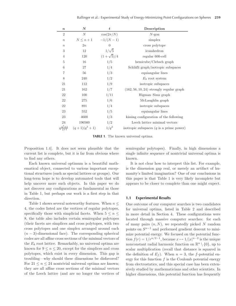
A list of all known universal optima is given in Table 1.Here n is the dimension of the Euclidean space, N is thenumber of points, and t is the greatest inner product be-tween distinct points in the configuration (i.e., the cosineof the minimal angle). For detailed descriptions of theseconfigurations, see [Cohn and Kumar 07, Section 1].
Each known universal optimum is uniquely deter-mined by the parameters listed in Table 1, except forthe configurations listed on the last line. For that case,when q = p� with p an odd prime, there are at least�(�−1)/2� distinct universal optima (see [Cameron et al.78] and [Kantor 86]). Classifying these optima is equiva-lent to classifying generalized quadrangles with parame-ters (q, q2), which is a difficult problem in combinatorics.In the other cases from Table 1, when uniqueness holds,we use the notation UN,n for the unique N -point univer-sal optimum in Rn.
Each of the configurations in Table 1 had been studiedbefore it appeared in [Cohn and Kumar 07], and wasalready known to be an optimal spherical code. In fact,when N ≥ 2n + 1 and n > 4, the codes on this list areexactly those that have been proved optimal. Cohn andKumar were unable to determine whether Table 1 is thecomplete list of universally optimal codes, except whenn ≤ 3.
All that is known in general is that any new universaloptimum must have N ≥ 2n + 1 [Cohn and Kumar 07,
Ballinger et al.: Experimental Study of Energy-Minimizing Point Configurations on Spheres 259
n N t Description
2 N cos(2π/N) N-gon
n N ≤ n+ 1 −1/(N − 1) simplex
n 2n 0 cross polytope
3 12 1/√
5 icosahedron
4 120 (1 +√
5)/4 regular 600-cell
5 16 1/5 hemicube/Clebsch graph
6 27 1/4 Schlafli graph/isotropic subspaces
7 56 1/3 equiangular lines
8 240 1/2 E8 root system
21 112 1/9 isotropic subspaces
21 162 1/7 (162, 56, 10, 24) strongly regular graph
22 100 1/11 Higman–Sims graph
22 275 1/6 McLaughlin graph
22 891 1/4 isotropic subspaces
23 552 1/5 equiangular lines
23 4600 1/3 kissing configuration of the following
24 196560 1/2 Leech lattice minimal vectors
q q3+1q+1
(q + 1)(q3 + 1) 1/q2 isotropic subspaces (q is a prime power)
TABLE 1. The known universal optima.
Proposition 1.4]. It does not seem plausible that thecurrent list is complete, but it is far from obvious whereto find any others.
Each known universal optimum is a beautiful math-ematical object, connected to various important excep-tional structures (such as special lattices or groups). Ourlong-term hope is to develop automated tools that willhelp uncover more such objects. In this paper we donot discover any configurations as fundamental as thosein Table 1, but perhaps our work is a first step in thatdirection.
Table 1 shows several noteworthy features. When n ≤4, the codes listed are the vertices of regular polytopes,specifically those with simplicial facets. When 5 ≤ n ≤8, the table also includes certain semiregular polytopes(their facets are simplices and cross polytopes, with twocross polytopes and one simplex arranged around each(n − 3)-dimensional face). The corresponding sphericalcodes are all affine cross sections of the minimal vectors ofthe E8 root lattice. Remarkably, no universal optima areknown for 9 ≤ n ≤ 20, except for the simplices and crosspolytopes, which exist in every dimension. This gap istroubling—why should these dimensions be disfavored?For 21 ≤ n ≤ 24 nontrivial universal optima are known;they are all affine cross sections of the minimal vectorsof the Leech lattice (and are no longer the vertices of
semiregular polytopes). Finally, in high dimensions asingle infinite sequence of nontrivial universal optima isknown.
It is not clear how to interpret this list. For example,is the dimension gap real, or merely an artifact of hu-manity’s limited imagination? One of our conclusions inthis paper is that Table 1 is very likely incomplete butappears to be closer to complete than one might expect.
1.1 Experimental Results
One outcome of our computer searches is two candidatesfor universal optima, listed in Table 2 and describedin more detail in Section 4. These configurations werelocated through massive computer searches: for eachof many pairs (n, N), we repeatedly picked N randompoints on Sn−1 and performed gradient descent to mini-mize potential energy. We focused on the potential func-tion f(r) = 1/rn/2−1, because x → 1/|x|n−2 is the uniquenonconstant radial harmonic function on Rn \ {0}, up toscalar multiplication (recall that distance is squared inthe definition of Ef ). When n = 3, the f -potential en-ergy for this function f is the Coulomb potential energyfrom electrostatics, and this special case has been exten-sively studied by mathematicians and other scientists. Inhigher dimensions, this potential function has frequently

260 Experimental Mathematics, Vol. 18 (2009), No. 3
n N t References
10 40 1/6 [Sloane 00, Hovinga 04]14 64 1/7 [Nordstrom and Robinson 67, de Caen and van Dam 99, Ericson and Zinoviev 01]
TABLE 2. New conjectured universal optima.
been studied as a natural generalization of electrostatics;we call it the harmonic potential function.
Because there are typically numerous local minimafor harmonic energy, we repeated this optimization pro-cedure many times with the hope of finding the globalminimum. For low numbers of points in low dimensions,the apparent global minimum occurs fairly frequently.Figure 1 shows data from three dimensions. In higherdimensions, there are usually more local minima and thetrue optimum can occur very infrequently.
For each conjectured optimum for harmonic energy,we attempted to determine whether it could be uni-versally optimal. We first determined whether it isin equilibrium under all possible force laws (i.e., “bal-anced” in the terminology of Leech [Leech 57]). Thatholds if and only if for each point x in the configu-ration and each distance d, the sum of all points inthe code at distance d from x is a scalar multiple ofx. If this criterion fails, then there is some inversepower law under which the code is not even in equilib-rium, let alone globally minimal, so it cannot possiblybe universally optimal. Most of the time, the code withthe lowest harmonic potential energy is not balanced.When it is balanced, we compared several potential func-tions to see whether we could disprove universal opti-mality. By [Widder 41, Theorem 9b, p. 154], it suf-fices to look at the potential functions f(r) = (4 − r)k
with k ∈ {0, 1, 2, . . .} (on each compact subinterval of(0, 4], every completely monotonic function can be ap-proximated arbitrarily closely by positive linear com-binations of these potential functions). Because thesefunctions do not blow up at r = 0, numerical cal-culations with them often converge more slowly thanthey do for inverse power laws (nearby points can ex-
Pro
babi
lity
0
1
2 64Number of points
FIGURE 1. Probabilities of local minima for harmonicenergy in R
3 (based on 1000 trials). White circlesdenote the conjectured harmonic optima.
perience only a bounded force pushing them apart),so they are not a convenient choice for initial experi-mentation. However, they play a fundamental role indetecting universal optima.
To date, our search has led us to 58 balanced config-urations with at most 64 points (and at least 2n + 1 indimension n) that appear to minimize harmonic energyand were not already known to be universally optimal.In all but two cases, we were able to disprove universaloptimality, but the remaining two cases (those listed inTable 2) are unresolved. We conjecture that they are infact universally optimal.
Figure 2 presents a graphical overview of our data.The triangle of white circles on the upper left representsthe simplices, and the diagonal line of white circles rep-resents the cross polytopes. Between them, one can seethat the pattern is fairly regular, but as one moves rightfrom the cross polytopes all structure rapidly vanishes.There is little hope of finding a simple method to predictwhere balanced harmonic optima can be found, let aloneuniversal optima. It also does not seem likely that gen-eral universal optima can be characterized by any variantof Cohn and Kumar’s criterion.
Besides the isotropic subspace universal optima fromTable 1 and the other universal optima with the sameparameters, we can conjecture only one infinite familyof balanced harmonic optima with more than 2n points
Dim
ensi
on
32
32 Number of points 64
FIGURE 2. Status of conjectured harmonic optimawith up to 64 points in at most 32 dimensions: whitecircle denotes universal optimum, large gray circle de-notes conjectured universal optimum, black circle de-notes balanced configuration that is not universallyoptimal, tiny black circle denotes unbalanced configu-ration.
Ballinger et al.: Experimental Study of Energy-Minimizing Point Configurations on Spheres 261
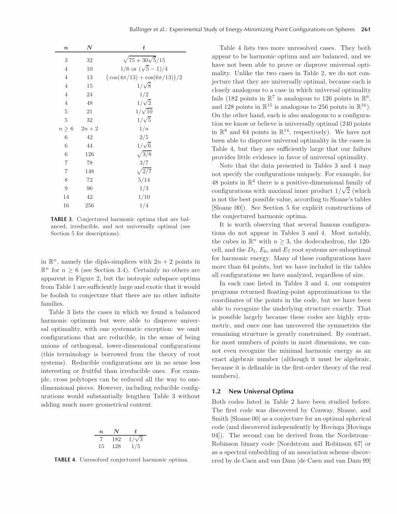
n N t
3 32√
75 + 30√
5/15
4 10 1/6 or (√
5 − 1)/4
4 13(cos(4π/13) + cos(6π/13)
)/2
4 15 1/√
8
4 24 1/2
4 48 1/√
2
5 21 1/√
10
5 32 1/√
5
n ≥ 6 2n+ 2 1/n
6 42 2/5
6 44 1/√
6
6 126√
3/8
7 78 3/7
7 148√
2/7
8 72 5/14
9 96 1/3
14 42 1/10
16 256 1/4
TABLE 3. Conjectured harmonic optima that are bal-anced, irreducible, and not universally optimal (seeSection 5 for descriptions).
in Rn, namely the diplo-simplices with 2n + 2 points inRn for n ≥ 6 (see Section 3.4). Certainly no others areapparent in Figure 2, but the isotropic subspace optimafrom Table 1 are sufficiently large and exotic that it wouldbe foolish to conjecture that there are no other infinitefamilies.
Table 3 lists the cases in which we found a balancedharmonic optimum but were able to disprove univer-sal optimality, with one systematic exception: we omitconfigurations that are reducible, in the sense of beingunions of orthogonal, lower-dimensional configurations(this terminology is borrowed from the theory of rootsystems). Reducible configurations are in no sense lessinteresting or fruitful than irreducible ones. For exam-ple, cross polytopes can be reduced all the way to one-dimensional pieces. However, including reducible config-urations would substantially lengthen Table 3 withoutadding much more geometrical content.
n N t
7 182 1/√
315 128 1/5
TABLE 4. Unresolved conjectured harmonic optima.
Table 4 lists two more unresolved cases. They bothappear to be harmonic optima and are balanced, and wehave not been able to prove or disprove universal opti-mality. Unlike the two cases in Table 2, we do not con-jecture that they are universally optimal, because each isclosely analogous to a case in which universal optimalityfails (182 points in R
7 is analogous to 126 points in R6,and 128 points in R15 is analogous to 256 points in R16).On the other hand, each is also analogous to a configura-tion we know or believe is universally optimal (240 pointsin R8 and 64 points in R14, respectively). We have notbeen able to disprove universal optimality in the cases inTable 4, but they are sufficiently large that our failureprovides little evidence in favor of universal optimality.
Note that the data presented in Tables 3 and 4 maynot specify the configurations uniquely. For example, for48 points in R4 there is a positive-dimensional family ofconfigurations with maximal inner product 1/
√2 (which
is not the best possible value, according to Sloane’s tables[Sloane 00]). See Section 5 for explicit constructions ofthe conjectured harmonic optima.
It is worth observing that several famous configura-tions do not appear in Tables 3 and 4. Most notably,the cubes in R
n with n ≥ 3, the dodecahedron, the 120-cell, and the D5, E6, and E7 root systems are suboptimalfor harmonic energy. Many of these configurations havemore than 64 points, but we have included in the tablesall configurations we have analyzed, regardless of size.
In each case listed in Tables 3 and 4, our computerprograms returned floating-point approximations to thecoordinates of the points in the code, but we have beenable to recognize the underlying structure exactly. Thatis possible largely because these codes are highly sym-metric, and once one has uncovered the symmetries theremaining structure is greatly constrained. By contrast,for most numbers of points in most dimensions, we can-not even recognize the minimal harmonic energy as anexact algebraic number (although it must be algebraic,because it is definable in the first-order theory of the realnumbers).
1.2 New Universal Optima
Both codes listed in Table 2 have been studied before.The first code was discovered by Conway, Sloane, andSmith [Sloane 00] as a conjecture for an optimal sphericalcode (and discovered independently by Hovinga [Hovinga04]). The second can be derived from the Nordstrom–Robinson binary code [Nordstrom and Robinson 67] oras a spectral embedding of an association scheme discov-ered by de Caen and van Dam [de Caen and van Dam 99]
262 Experimental Mathematics, Vol. 18 (2009), No. 3
(take t = 1 in [de Caen and van Dam 99, Theorem 2 andProposition 7(i)] and then project the standard orthonor-mal basis into a common eigenspace of the operators inthe Bose–Mesner algebra of the association scheme). Wedescribe both codes in greater detail in Section 4.
Neither code satisfies the condition from [Cohn andKumar 07] for universal optimality: both are spherical 3-designs (but not 4-designs), with four distances betweendistinct points in the 40-point code and three in the 64-point code. That leaves open the possibility of an adhoc proof, similar to the one Cohn and Kumar gave forthe regular 600-cell, but the techniques from [Cohn andKumar 07] do not apply.
To test universal optimality, we have carried out 1000random trials with the potential function f(r) = (4 −r)k for each k from 1 to 25. We have also carried out1000 trials using Hardin and Sloane’s program Gosset[Hardin and Sloane 03] to construct good spherical codes(to take care of the case when k is large). Of course theseexperimental tests fall far short of a rigorous proof, butthe codes certainly appear to be universally optimal.
We believe that they are the only possible new univer-sal optima consisting of at most 64 points, because wehave searched the space of such codes fairly thoroughly.By [Cohn and Kumar 07, Proposition 1.4], any new uni-versal optimum in R
n must contain at least 2n+1 points.There are 812 such cases with at most 64 points in di-mension at least 4. In each case, we have completed atleast 1000 random trials (and usually more). There isno guarantee that we have found the global optimum inany of these cases, because it could have a tiny basin ofattraction. However, a simple calculation shows that itis 99.99% likely that in every case we have found everylocal minimum that occurs at least 2% of the time. Wehave probably not always found the true optimum, butwe believe that we have found every universal optimumwithin the range we have searched.
We have made our tables of conjectured harmonic op-tima for up to 64 points in up to 32 dimensions availablevia the world wide web.1 They list the best energieswe have found and the coordinates of the configurationsthat achieve them. We would be grateful for any im-provements, and we intend to keep the tables up to date,with credit for any contributions received from others.
In addition to carrying out our own searches for uni-versal optima, we have examined Sloane’s tables [Sloane00] of the best spherical codes known with at most 130points in R
4 and R5, and we have verified that they con-
1Available at http://aimath.org/data/paper/BBCGKS2006/.
tain no new universal optima. We strongly suspect thatthere are no undiscovered universal optima of any size inR4 or R5, based on Sloane’s calculations as well as oursearches, but it would be difficult to give definitive ex-perimental evidence for such an assertion (we see no con-vincing arguments for why huge universal optima shouldnot exist).
In general, our searches among larger codes have beenfar less exhaustive than those up to 64 points: we haveat least briefly examined well over four thousand differ-ent pairs (n, N), but generally not in sufficient depth tomake a compelling case that we have found the globalminimum. (Every time we found a balanced harmonicoptimum, with the exception of 128 points in R15 and256 points in R16, we completed at least 1000 trials totest whether it was really optimal. However, we have notcompleted nearly as many trials in most other cases, andin any case 1000 trials is not enough when one is studyinglarge configurations.) Nevertheless, our strong impres-sion is that universal optima are rare, and certainly thatthere are few small universal optima with large basins ofattraction.
2. METHODOLOGY
2.1 Techniques
As discussed in the introduction, to minimize potentialenergy we apply gradient descent, starting from manyrandom initial configurations. That is an unsophisticatedapproach, because gradient descent is known to performmore slowly in many situations than competing meth-ods such as the conjugate gradient algorithm. However,it has performed adequately in our computations. Fur-thermore, gradient descent has particularly intuitive dy-namics. Imagine particles immersed in a medium withenough viscosity that they never build up momentum.When a force acts on them according to the potentialfunction, the configuration undergoes gradient descent.By contrast, for most other optimization methods themotion of the particles is more obscure, so for example itis more difficult to interpret information such as sizes ofbasins of attraction.
Once we have approximate coordinates, we can use themultivariate analogue of Newton’s method to computethem to high precision (by searching for a zero of thegradient vector). Usually we do not need to do this, be-cause the results of gradient descent are accurate enoughfor our purposes, but it is a useful tool to have available.
Obtaining coordinates is simply the beginning of ouranalysis. Because the coordinates encode not only the
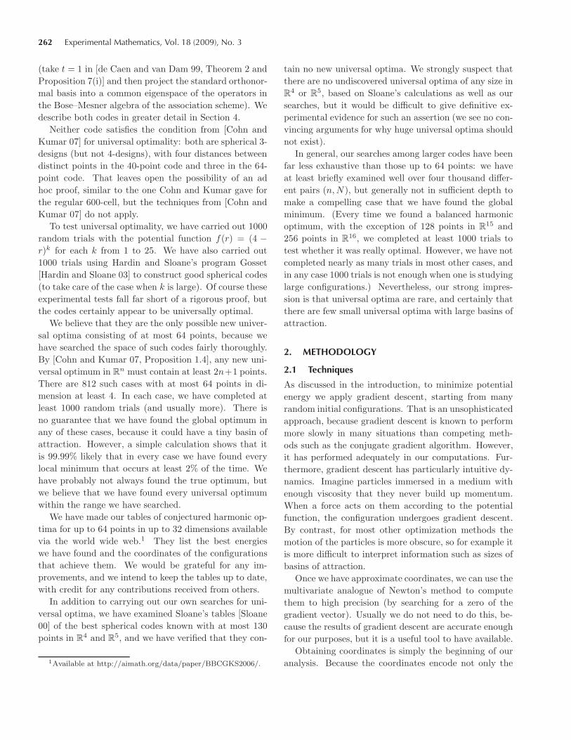
Ballinger et al.: Experimental Study of Energy-Minimizing Point Configurations on Spheres 263
FIGURE 3. The Gram matrix for a regular 600-cell(black denotes 1, white denotes −1, and gray inter-polates between them), with the points ordered as re-turned by our gradient descent software.
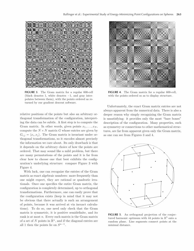
relative positions of the points but also an arbitrary or-thogonal transformation of the configuration, interpret-ing the data can be subtle. A first step is to compute theGram matrix. In other words, given points x1, . . . , xN ,compute the N ×N matrix G whose entries are given byGi,j = 〈xi, xj〉. The Gram matrix is invariant under or-thogonal transformations, so it encodes almost preciselythe information we care about. Its only drawback is thatit depends on the arbitrary choice of how the points areordered. That may sound like a mild problem, but thereare many permutations of the points and it is far fromclear how to choose one that best exhibits the config-uration’s underlying structure: compare Figure 3 withFigure 4.
With luck, one can recognize the entries of the Grammatrix as exact algebraic numbers: more frequently thanone might expect, they are rational or quadratic irra-tionals. Once one specifies the entire Gram matrix, theconfiguration is completely determined, up to orthogonaltransformations. Furthermore, one can easily prove thatthe configuration exists (keep in mind that it may notbe obvious that there actually is such an arrangementof points, because it was arrived at via inexact calcula-tions). To do so, one need only check that the Grammatrix is symmetric, it is positive semidefinite, and itsrank is at most n. Every such matrix is the Gram matrixof a set of N points in R
n, and if the diagonal entries areall 1 then the points lie on Sn−1.
FIGURE 4. The Gram matrix for a regular 600-cell,with the points ordered so as to display structure.
Unfortunately, the exact Gram matrix entries are notalways apparent from the numerical data. There is also adeeper reason why simply recognizing the Gram matrixis unsatisfying: it provides only the most “bare bones”description of the configuration. Many properties, suchas symmetry or connections to other mathematical struc-tures, are far from apparent given only the Gram matrix,as one can see from Figures 3 and 4.
FIGURE 5. An orthogonal projection of the conjec-tured harmonic optimum with 44 points in R
3 onto arandom plane. Line segments connect points at theminimal distance.
264 Experimental Mathematics, Vol. 18 (2009), No. 3
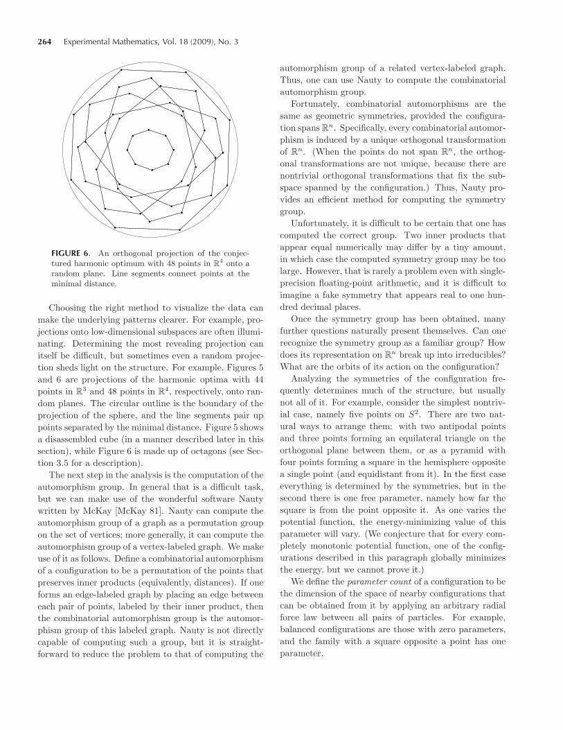
FIGURE 6. An orthogonal projection of the conjec-tured harmonic optimum with 48 points in R
4 onto arandom plane. Line segments connect points at theminimal distance.
Choosing the right method to visualize the data canmake the underlying patterns clearer. For example, pro-jections onto low-dimensional subspaces are often illumi-nating. Determining the most revealing projection canitself be difficult, but sometimes even a random projec-tion sheds light on the structure. For example, Figures 5and 6 are projections of the harmonic optima with 44points in R
3 and 48 points in R4, respectively, onto ran-dom planes. The circular outline is the boundary of theprojection of the sphere, and the line segments pair uppoints separated by the minimal distance. Figure 5 showsa disassembled cube (in a manner described later in thissection), while Figure 6 is made up of octagons (see Sec-tion 3.5 for a description).
The next step in the analysis is the computation of theautomorphism group. In general that is a difficult task,but we can make use of the wonderful software Nautywritten by McKay [McKay 81]. Nauty can compute theautomorphism group of a graph as a permutation groupon the set of vertices; more generally, it can compute theautomorphism group of a vertex-labeled graph. We makeuse of it as follows. Define a combinatorial automorphismof a configuration to be a permutation of the points thatpreserves inner products (equivalently, distances). If oneforms an edge-labeled graph by placing an edge betweeneach pair of points, labeled by their inner product, thenthe combinatorial automorphism group is the automor-phism group of this labeled graph. Nauty is not directlycapable of computing such a group, but it is straight-forward to reduce the problem to that of computing the
automorphism group of a related vertex-labeled graph.Thus, one can use Nauty to compute the combinatorialautomorphism group.
Fortunately, combinatorial automorphisms are thesame as geometric symmetries, provided the configura-tion spans R
n. Specifically, every combinatorial automor-phism is induced by a unique orthogonal transformationof Rn. (When the points do not span Rn, the orthog-onal transformations are not unique, because there arenontrivial orthogonal transformations that fix the sub-space spanned by the configuration.) Thus, Nauty pro-vides an efficient method for computing the symmetrygroup.
Unfortunately, it is difficult to be certain that one hascomputed the correct group. Two inner products thatappear equal numerically may differ by a tiny amount,in which case the computed symmetry group may be toolarge. However, that is rarely a problem even with single-precision floating-point arithmetic, and it is difficult toimagine a fake symmetry that appears real to one hun-dred decimal places.
Once the symmetry group has been obtained, manyfurther questions naturally present themselves. Can onerecognize the symmetry group as a familiar group? Howdoes its representation on R
n break up into irreducibles?What are the orbits of its action on the configuration?
Analyzing the symmetries of the configuration fre-quently determines much of the structure, but usuallynot all of it. For example, consider the simplest nontriv-ial case, namely five points on S2. There are two nat-ural ways to arrange them: with two antipodal pointsand three points forming an equilateral triangle on theorthogonal plane between them, or as a pyramid withfour points forming a square in the hemisphere oppositea single point (and equidistant from it). In the first caseeverything is determined by the symmetries, but in thesecond there is one free parameter, namely how far thesquare is from the point opposite it. As one varies thepotential function, the energy-minimizing value of thisparameter will vary. (We conjecture that for every com-pletely monotonic potential function, one of the config-urations described in this paragraph globally minimizesthe energy, but we cannot prove it.)
We define the parameter count of a configuration to bethe dimension of the space of nearby configurations thatcan be obtained from it by applying an arbitrary radialforce law between all pairs of particles. For example,balanced configurations are those with zero parameters,and the family with a square opposite a point has oneparameter.
Ballinger et al.: Experimental Study of Energy-Minimizing Point Configurations on Spheres 265
To compute the parameter count for an N -point con-figuration, start by viewing it as an element of (Sn−1)N
(by ordering the points). Within the tangent space ofthis manifold, for each radial force law there is a tangentvector. To form a basis for all these force vectors, lookat all distances d that occur in the configuration, andfor each of them consider the tangent vector that pusheseach pair of points at distance d in opposite directions buthas no other effects. All force vectors are linear combina-tions of these, and the dimension of the space they spanis the parameter count for the configuration. (One mustbe careful to use sufficiently high-precision arithmetic, aswhen computing the symmetry group.)
This information is useful because in a sense it showshow much humanly understandable structure we can ex-pect to find. For example, in the five-point configura-tion with a square opposite a point, the distance be-tween them will typically be some complicated numberdepending on the potential function. In principle onecan describe it exactly, but in practice it is most pleas-ant to treat it as a black box and describe all the otherdistances in the configuration in terms of it. The param-eter count tells how many independent parameters oneshould expect to arrive at. When the count is zero orone, it is reasonable to search for an elegant description,whereas when the count is twenty, it is likely that theconfiguration is unavoidably complex.
Figure 7 shows the parameter counts of the conjec-tured harmonic optima in R
3 with at most 64 points,compared with the dimension of the full space of all con-figurations of their size. The counts vary wildly but areoften quite a bit smaller than one might expect. Twostriking examples are 61 points with 111 parameters, forwhich there is likely no humanly understandable descrip-tion, and 44 points with one parameter. The 44-pointconfiguration consists of the vertices of a cube and cen-ters of its edges together with the 24-point orbit (underthe cube’s symmetry group) of a point on a diagonal ofa face, all projected onto a common sphere. The optimalchoice of the point on the diagonal appears complicated.
One subtlety in searching for local minima is that anygiven potential function will usually not detect all pos-sible families of local minima that could occur for otherpotential functions. For example, for five points in R
3,the family with a square opposite a point does not con-tain a local minimum for harmonic energy. One canattain a local minimum compared to the other mem-bers of the family, but it will be a saddle point in thespace of all configurations. Nevertheless, the family doescontain local minima for some other completely mono-
Par
amet
er c
ount
0
130
2 64Number of points
FIGURE 7. Parameter counts for conjectured har-monic optima in R
3. Horizontal or vertical lines occurat multiples of ten, and white circles denote the di-mension of the configuration space.
tonic potential functions (such as f(r) = 1/rs withs large).
2.2 Example
For a concrete example, consider Table 5, which showsthe results of 108 random trials for 27 points in R6 (alldecimal numbers in tables have been rounded). Theseparameters were chosen because, as shown in [Cohn andKumar 07], there is a unique 27-point universal optimumin R6, with harmonic energy 111; it is called the Schlafliconfiguration. The column labeled “frequency” tells howmany times each local minimum occurred. As one cansee, the universal optimum occurred more than 99.97%of the time, but we found a total of four others.
Strictly speaking, we have not proved that the localminima listed in Table 5 (other than the Schlafli configu-ration) even exist. They surely do, because we have com-puted them to five hundred decimal places and checkedthat they are local minima by numerically diagonalizingthe Hessian matrix of the energy function on the space ofconfigurations. However, we used high-precision floating-point arithmetic, so this calculation does not constitutea rigorous proof, although it leaves no reasonable doubt.It is not at all clear whether there are additional localminima. We have not found any, but the fact that oneof the local minima occurs only once in every ten mil-lion trials suggests that there might be others with evensmaller basins of attraction.
The local minimum with energy 112.736 . . . stands outin two respects besides its extreme rarity: it has manysymmetries and it depends on few parameters. That sug-
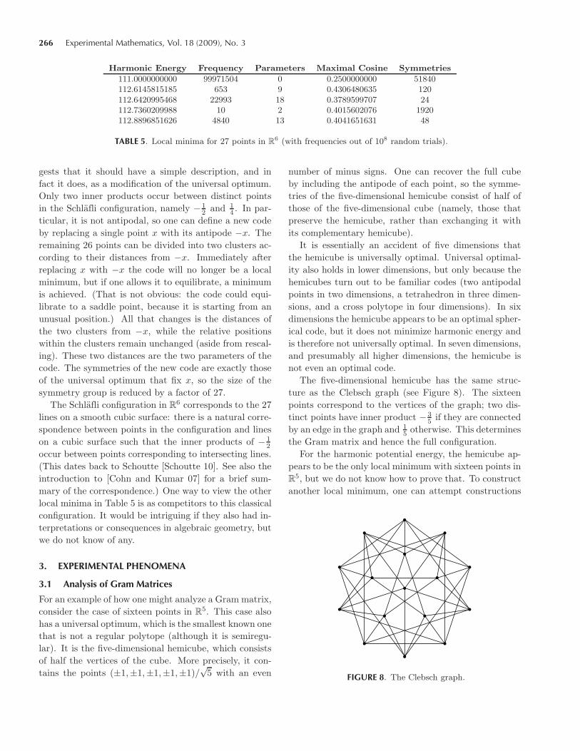
266 Experimental Mathematics, Vol. 18 (2009), No. 3
Harmonic Energy Frequency Parameters Maximal Cosine Symmetries
111.0000000000 99971504 0 0.2500000000 51840112.6145815185 653 9 0.4306480635 120112.6420995468 22993 18 0.3789599707 24112.7360209988 10 2 0.4015602076 1920112.8896851626 4840 13 0.4041651631 48
TABLE 5. Local minima for 27 points in R6 (with frequencies out of 108 random trials).
gests that it should have a simple description, and infact it does, as a modification of the universal optimum.Only two inner products occur between distinct pointsin the Schlafli configuration, namely − 1
2 and 14 . In par-
ticular, it is not antipodal, so one can define a new codeby replacing a single point x with its antipode −x. Theremaining 26 points can be divided into two clusters ac-cording to their distances from −x. Immediately afterreplacing x with −x the code will no longer be a localminimum, but if one allows it to equilibrate, a minimumis achieved. (That is not obvious: the code could equi-librate to a saddle point, because it is starting from anunusual position.) All that changes is the distances ofthe two clusters from −x, while the relative positionswithin the clusters remain unchanged (aside from rescal-ing). These two distances are the two parameters of thecode. The symmetries of the new code are exactly thoseof the universal optimum that fix x, so the size of thesymmetry group is reduced by a factor of 27.
The Schlafli configuration in R6 corresponds to the 27
lines on a smooth cubic surface: there is a natural corre-spondence between points in the configuration and lineson a cubic surface such that the inner products of − 1
2
occur between points corresponding to intersecting lines.(This dates back to Schoutte [Schoutte 10]. See also theintroduction to [Cohn and Kumar 07] for a brief sum-mary of the correspondence.) One way to view the otherlocal minima in Table 5 is as competitors to this classicalconfiguration. It would be intriguing if they also had in-terpretations or consequences in algebraic geometry, butwe do not know of any.
3. EXPERIMENTAL PHENOMENA
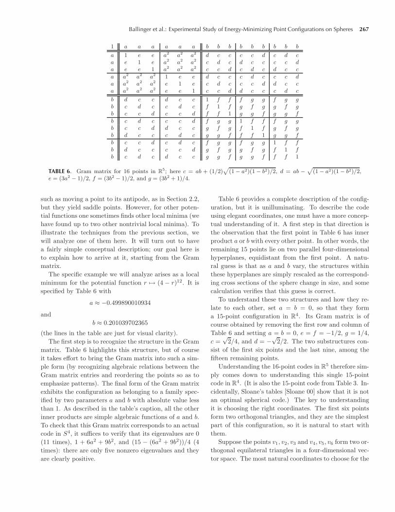
3.1 Analysis of Gram Matrices
For an example of how one might analyze a Gram matrix,consider the case of sixteen points in R
5. This case alsohas a universal optimum, which is the smallest known onethat is not a regular polytope (although it is semiregu-lar). It is the five-dimensional hemicube, which consistsof half the vertices of the cube. More precisely, it con-tains the points (±1,±1,±1,±1,±1)/
√5 with an even
number of minus signs. One can recover the full cubeby including the antipode of each point, so the symme-tries of the five-dimensional hemicube consist of half ofthose of the five-dimensional cube (namely, those thatpreserve the hemicube, rather than exchanging it withits complementary hemicube).
It is essentially an accident of five dimensions thatthe hemicube is universally optimal. Universal optimal-ity also holds in lower dimensions, but only because thehemicubes turn out to be familiar codes (two antipodalpoints in two dimensions, a tetrahedron in three dimen-sions, and a cross polytope in four dimensions). In sixdimensions the hemicube appears to be an optimal spher-ical code, but it does not minimize harmonic energy andis therefore not universally optimal. In seven dimensions,and presumably all higher dimensions, the hemicube isnot even an optimal code.
The five-dimensional hemicube has the same struc-ture as the Clebsch graph (see Figure 8). The sixteenpoints correspond to the vertices of the graph; two dis-tinct points have inner product − 3
5 if they are connectedby an edge in the graph and 1
5 otherwise. This determinesthe Gram matrix and hence the full configuration.
For the harmonic potential energy, the hemicube ap-pears to be the only local minimum with sixteen points inR5, but we do not know how to prove that. To constructanother local minimum, one can attempt constructions
FIGURE 8. The Clebsch graph.
Ballinger et al.: Experimental Study of Energy-Minimizing Point Configurations on Spheres 267
1 a a a a a a b b b b b b b b b
a 1 e e a2 a2 a2 d c c c c d c d ca e 1 e a2 a2 a2 c d c d c c c c da e e 1 a2 a2 a2 c c d c d c d c c
a a2 a2 a2 1 e e d c c c d c c c da a2 a2 a2 e 1 e c d c c c d d c ca a2 a2 a2 e e 1 c c d d c c c d c
b d c c d c c 1 f f f g g f g gb c d c c d c f 1 f g f g g f gb c c d c c d f f 1 g g f g g f
b c d c c c d f g g 1 f f f g gb c c d d c c g f g f 1 f g f gb d c c c d c g g f f f 1 g g f
b c c d c d c f g g f g g 1 f fb d c c c c d g f g g f g f 1 fb c d c d c c g g f g g f f f 1
TABLE 6. Gram matrix for 16 points in R5; here c = ab + (1/2)
√(1 − a2)(1 − b2)/2, d = ab − √
(1 − a2)(1 − b2)/2,e = (3a2 − 1)/2, f = (3b2 − 1)/2, and g = (3b2 + 1)/4.
such as moving a point to its antipode, as in Section 2.2,but they yield saddle points. However, for other poten-tial functions one sometimes finds other local minima (wehave found up to two other nontrivial local minima). Toillustrate the techniques from the previous section, wewill analyze one of them here. It will turn out to havea fairly simple conceptual description; our goal here isto explain how to arrive at it, starting from the Grammatrix.
The specific example we will analyze arises as a localminimum for the potential function r → (4 − r)12. It isspecified by Table 6 with
a ≈ −0.499890010934
andb ≈ 0.201039702365
(the lines in the table are just for visual clarity).The first step is to recognize the structure in the Gram
matrix. Table 6 highlights this structure, but of courseit takes effort to bring the Gram matrix into such a sim-ple form (by recognizing algebraic relations between theGram matrix entries and reordering the points so as toemphasize patterns). The final form of the Gram matrixexhibits the configuration as belonging to a family spec-ified by two parameters a and b with absolute value lessthan 1. As described in the table’s caption, all the otherinner products are simple algebraic functions of a and b.To check that this Gram matrix corresponds to an actualcode in S4, it suffices to verify that its eigenvalues are 0(11 times), 1 + 6a2 + 9b2, and (15 − (6a2 + 9b2))/4 (4times): there are only five nonzero eigenvalues and theyare clearly positive.
Table 6 provides a complete description of the config-uration, but it is unilluminating. To describe the codeusing elegant coordinates, one must have a more concep-tual understanding of it. A first step in that direction isthe observation that the first point in Table 6 has innerproduct a or b with every other point. In other words, theremaining 15 points lie on two parallel four-dimensionalhyperplanes, equidistant from the first point. A natu-ral guess is that as a and b vary, the structures withinthese hyperplanes are simply rescaled as the correspond-ing cross sections of the sphere change in size, and somecalculation verifies that this guess is correct.
To understand these two structures and how they re-late to each other, set a = b = 0, so that they forma 15-point configuration in R
4. Its Gram matrix is ofcourse obtained by removing the first row and column ofTable 6 and setting a = b = 0, e = f = −1/2, g = 1/4,c =
√2/4, and d = −√
2/2. The two substructures con-sist of the first six points and the last nine, among thefifteen remaining points.
Understanding the 16-point codes in R5 therefore sim-
ply comes down to understanding this single 15-pointcode in R4. (It is also the 15-point code from Table 3. In-cidentally, Sloane’s tables [Sloane 00] show that it is notan optimal spherical code.) The key to understandingit is choosing the right coordinates. The first six pointsform two orthogonal triangles, and they are the simplestpart of this configuration, so it is natural to start withthem.
Suppose the points v1, v2, v3 and v4, v5, v6 form two or-thogonal equilateral triangles in a four-dimensional vec-tor space. The most natural coordinates to choose for the
268 Experimental Mathematics, Vol. 18 (2009), No. 3
1 c c d b b −2a a a −2a a ac 1 c b d b a −2a a a −2a ac c 1 b b d a a −2a a a −2a
d b b 1 c c −2a a a −2a a ab d b c 1 c a −2a a a −2a ab b d c c 1 a a −2a a a −2a
−2a a a −2a a a 1 c c d b ba −2a a a −2a a c 1 c b d ba a −2a a a −2a c c 1 b b d
−2a a a −2a a a d b b 1 c ca −2a a a −2a a b d b c 1 ca a −2a a a −2a b b d c c 1
TABLE 7. Gram matrix for 12 points in R4; here 0 < a < 1
2, b = a− 1, c = −3a+ 1, and d = 4a− 1.
vector space are the inner products with these six points.Of course the sum of the three inner products with anytriangle must vanish (because v1+v2+v3 = v4+v5+v6 =0), so there are only four independent coordinates, butwe prefer not to break the symmetry by discarding twocoordinates.
The other nine points in the configuration are deter-mined by their inner products with v1, . . . , v6. Eachof them will have inner product d with one point ineach triangle and c with the remaining two points. Aspointed out above we must have d + 2c = 0, and in factd = −√
2/2 and c =√
2/4 because the points are all unitvectors. Note that one can read off all this informationfrom the c and d entries in Table 6.
There is an important conceptual point in the lastpart of this analysis. Instead of focusing on the internalstructure among the last nine points, it is most fruitfulto study how they relate to the previously understoodsubconfiguration of six points. However, once one hasa complete description, it is important to examine theinternal structure as well.
The pattern of connections among the last nine pointsin Table 6 is described by the Paley graph on nine ver-tices, which is the unique strongly regular graph withparameters (9, 4, 1, 2). (The Paley graph is isomorphicto its own complement, so the edges could correspondto inner product either f or g.) Strongly regular graphs,and more generally association schemes, frequently occuras substructures of minimal-energy configurations. It isremarkable to see such highly ordered structures sponta-neously occurring via energy minimization.
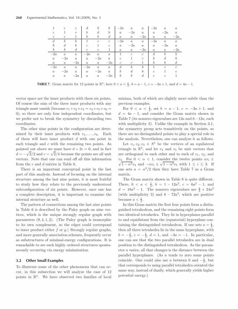
3.2 Other Small Examples
To illustrate some of the other phenomena that can oc-cur, in this subsection we will analyze the case of 12points in R
4. We have observed two families of local
minima, both of which are slightly more subtle than theprevious examples.
For 0 < a < 12 , set b = a − 1, c = −3a + 1, and
d = 4a − 1, and consider the Gram matrix shown inTable 7 (its nonzero eigenvalues are 12a and 6−12a, eachwith multiplicity 2). Unlike the example in Section 3.1,the symmetry group acts transitively on the points, sothere are no distinguished points to play a special role inthe analysis. Nevertheless, one can analyze it as follows.
Let v1, v2, v3 ∈ S1 be the vertices of an equilateraltriangle in R2, and let v4 and v5 be unit vectors thatare orthogonal to each other and to each of v1, v2, andv3. For 0 < α < 1, consider the twelve points αvi ±√
1 − α2v4 and −αvi ±√
1 − α2v5 with 1 ≤ i ≤ 3. Ifone sets a = α2/2 then they have Table 7 as a Grammatrix.
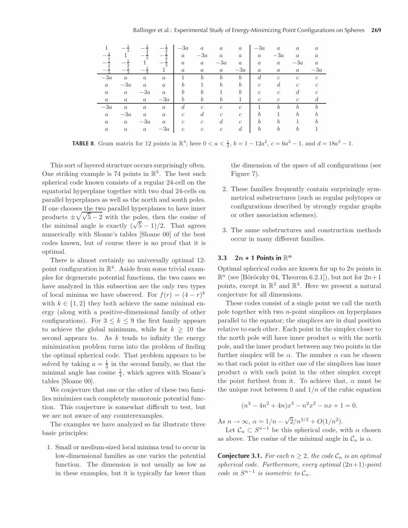
The Gram matrix shown in Table 8 is quite different.There, 0 < a < 1
3 , b = 1 − 12a2, c = 6a2 − 1, andd = 18a2 − 1. The nonzero eigenvalues are 4
3 + 24a2
(with multiplicity 3) and 8 − 72a2, which are positivebecause a < 1
3 .In this Gram matrix the first four points form a distin-
guished tetrahedron, and the remaining eight points formtwo identical tetrahedra. They lie in hyperplanes parallelto and equidistant from the (equatorial) hyperplane con-taining the distinguished tetrahedron. If one sets a = 1
3 ,then all three tetrahedra lie in the same hyperplane, withb = − 1
3 , c = − 13 , d = 1, and −3a = −1. In particular,
one can see that the two parallel tetrahedra are in dualposition to the distinguished tetrahedron. As the param-eter a varies, all that changes is the distance between theparallel hyperplanes. (As a tends to zero some pointscoincide. One could also use a between 0 and − 1
3 , butthat corresponds to using parallel tetrahedra oriented thesame way, instead of dually, which generally yields higherpotential energy.)
Ballinger et al.: Experimental Study of Energy-Minimizing Point Configurations on Spheres 269
1 − 13
− 13
− 13
−3a a a a −3a a a a− 1
31 − 1
3− 1
3a −3a a a a −3a a a
− 13
− 13
1 − 13
a a −3a a a a −3a a− 1
3− 1
3− 1
31 a a a −3a a a a −3a
−3a a a a 1 b b b d c c ca −3a a a b 1 b b c d c ca a −3a a b b 1 b c c d ca a a −3a b b b 1 c c c d
−3a a a a d c c c 1 b b ba −3a a a c d c c b 1 b ba a −3a a c c d c b b 1 ba a a −3a c c c d b b b 1
TABLE 8. Gram matrix for 12 points in R4; here 0 < a < 1
3, b = 1 − 12a2, c = 6a2 − 1, and d = 18a2 − 1.
This sort of layered structure occurs surprisingly often.One striking example is 74 points in R5. The best suchspherical code known consists of a regular 24-cell on theequatorial hyperplane together with two dual 24-cells onparallel hyperplanes as well as the north and south poles.If one chooses the two parallel hyperplanes to have innerproducts ±
√√5 − 2 with the poles, then the cosine of
the minimal angle is exactly (√
5 − 1)/2. That agreesnumerically with Sloane’s tables [Sloane 00] of the bestcodes known, but of course there is no proof that it isoptimal.
There is almost certainly no universally optimal 12-point configuration in R
4. Aside from some trivial exam-ples for degenerate potential functions, the two cases wehave analyzed in this subsection are the only two typesof local minima we have observed. For f(r) = (4 − r)k
with k ∈ {1, 2} they both achieve the same minimal en-ergy (along with a positive-dimensional family of otherconfigurations). For 3 ≤ k ≤ 9 the first family appearsto achieve the global minimum, while for k ≥ 10 thesecond appears to. As k tends to infinity the energyminimization problem turns into the problem of findingthe optimal spherical code. That problem appears to besolved by taking a = 1
4 in the second family, so that theminimal angle has cosine 1
4 , which agrees with Sloane’stables [Sloane 00].
We conjecture that one or the other of these two fami-lies minimizes each completely monotonic potential func-tion. This conjecture is somewhat difficult to test, butwe are not aware of any counterexamples.
The examples we have analyzed so far illustrate threebasic principles:
1. Small or medium-sized local minima tend to occur inlow-dimensional families as one varies the potentialfunction. The dimension is not usually as low asin these examples, but it is typically far lower than
the dimension of the space of all configurations (seeFigure 7).
2. These families frequently contain surprisingly sym-metrical substructures (such as regular polytopes orconfigurations described by strongly regular graphsor other association schemes).
3. The same substructures and construction methodsoccur in many different families.
3.3 2n + 1 Points in Rn
Optimal spherical codes are known for up to 2n points inRn (see [Boroczky 04, Theorem 6.2.1]), but not for 2n+1points, except in R2 and R3. Here we present a naturalconjecture for all dimensions.
These codes consist of a single point we call the northpole together with two n-point simplices on hyperplanesparallel to the equator; the simplices are in dual positionrelative to each other. Each point in the simplex closer tothe north pole will have inner product α with the northpole, and the inner product between any two points in thefurther simplex will be α. The number α can be chosenso that each point in either one of the simplices has innerproduct α with each point in the other simplex exceptthe point furthest from it. To achieve that, α must bethe unique root between 0 and 1/n of the cubic equation
(n3 − 4n2 + 4n)x3 − n2x2 − nx + 1 = 0.
As n → ∞, α = 1/n −√2/n3/2 + O(1/n2).
Let Cn ⊂ Sn−1 be this spherical code, with α chosenas above. The cosine of the minimal angle in Cn is α.
Conjecture 3.1. For each n ≥ 2, the code Cn is an optimalspherical code. Furthermore, every optimal (2n+1)-pointcode in Sn−1 is isometric to Cn.
270 Experimental Mathematics, Vol. 18 (2009), No. 3
On philosophical grounds it seems reasonable to ex-pect to be able to prove this conjecture: most of thedifficulty in packing problems comes from the idiosyn-crasies of particular spaces and dimensions, so when aphenomenon occurs systematically one expects a concep-tual reason for it. However, we have made no seriousprogress toward a proof.
One can also construct Cn as follows. Imagine addingone point to a regular cross polytope by placing it in thecenter of a facet. The vertices of that facet form a simplexequidistant from the new point, as do the vertices of theopposite facet. The structure is identical to the codeCn, except for the distances from the new point, and theproper distances can be obtained by allowing the code toequilibrate with respect to increasingly steep potentialfunctions.
It appears that for n > 2 these codes do not mini-mize harmonic energy, so they are not universally opti-mal. When n = 4, something remarkable occurs with the(conjectured) minimum for harmonic energy. That con-figuration consists of a regular pentagon together withtwo pairs of antipodal points that are orthogonal to eachother and the pentagon. If one uses gradient descentto minimize harmonic energy, it seems to converge withprobability 1 to this configuration, but the convergenceis very slow, much slower than for any other harmonicenergy minimum we have found. The reason is that thisconfiguration is a degenerate minimum for the harmonicenergy, in the sense that the Hessian matrix has morezero eigenvalues than one would expect.
Each of the nine points has three degrees of free-dom, so the Hessian matrix has twenty-seven eigenvalues.Specifically, they are 0 (ten times), 4, 7/4 (twice), 9/2(four times), 9 (twice), 25/8±√
209/8 (twice each), and31/8 ± √
161/8 (twice each). Six of the zero eigenvaluesare unsurprising, because they come from the problem’sinvariance under the six-dimensional Lie group O(4), butthe remaining four are surprising indeed.
The corresponding eigenvectors are infinitesimal dis-placements of the nine points that produce only a fourth-order change in energy, rather than the expected second-order change. To construct them, do not move the an-tipodal pairs of points at all, and move the pentagonpoints orthogonally to the plane of the pentagon. Eachmust be displaced by (1 − √
5)/2 times the sum of thedisplacements of its two neighbors. This yields a four-dimensional space of displacements, which are the sur-prising eigenvectors.
This example is noteworthy because it shows that har-monic energy is not always a Morse function on the space
of all configurations. One might hope to apply Morse the-ory to understand the relationship between critical pointsfor energy and the topology of the configuration space,but the existence of degenerate critical points could sub-stantially complicate this approach.
3.4 2n + 2 Points in Rn
After seeing a conjecture for the optimal (2n + 1)-pointcode in Sn−1, it is natural to wonder about 2n+2 points.A first guess is the union of a simplex and its dual sim-plex (in other words, the antipodal simplex), which wasnamed the diplo-simplex by Conway and Sloane [Conwayand Sloane 91]. One can prove using the linear program-ming bounds for real projective space that this code isthe unique optimal antipodal spherical code of its sizeand dimension (see [Conway and Sloane 99, Chapter 9]),but for n > 2 it is not even locally optimal as a sphericalcode (see Section 7) and we do not have a conjecture forthe true answer.
For the problem of minimizing harmonic energy, thediplo-simplex is suboptimal for 3 ≤ n ≤ 5 but appearsoptimal for all other n.
One particularly elegant case is n = 4. The midpointsof the edges of a regular simplex form a 10-point code inS3 with maximal inner product 1
6 , and Bachoc and Val-lentin [Bachoc and Vallentin 09] have proved that it isthe unique optimal spherical code. It is also the kissingconfiguration of the five-dimensional hemicube (the uni-versally optimal 16-point configuration in R5). In otherwords, it consists of the ten nearest neighbors of any pointin that code. This code appears to minimize harmonicenergy, but it is not the unique minimum: two orthogonalregular pentagons have the same harmonic energy.
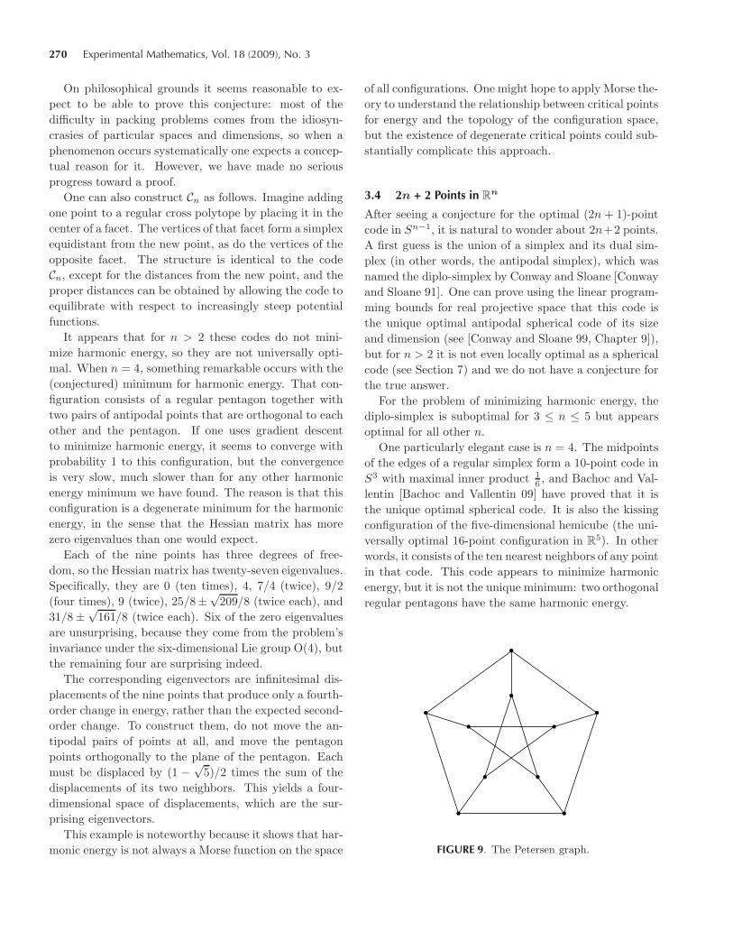
FIGURE 9. The Petersen graph.
Ballinger et al.: Experimental Study of Energy-Minimizing Point Configurations on Spheres 271
As pointed out in the introduction of [Cohn and Ku-mar 07], this code is not universally optimal, but it nev-ertheless seems to be an exceedingly interesting configu-ration. Only the inner products − 2
3 and 16 occur (besides
1, of course). If one forms a graph whose vertices are thepoints in the code and whose edges correspond to pairsof points with inner product − 2
3 , then the result is thefamous Petersen graph (Figure 9).
Like the nontrivial universal optima in dimensions 5through 8, this code consists of the vertices of a semireg-ular polytope that has simplices and cross polytopes asfacets, with a simplex and two cross polytopes meetingat each face of codimension 3. Its kissing configuration isalso semiregular, with square and triangular facets, butit is a suboptimal code (specifically, a triangular prism).
3.5 48 Points in R4
One of the most beautiful configurations we have found isa 48-point code in R4. The points form six octagons thatmap to the vertices of a regular octahedron under theHopf map from S3 to S2. Recall that if we identify R4
with C2 using the inner product 〈x, y〉 = Re xty on C2,then the Hopf map sends (z, w) to z/w ∈ C∪{∞}, whichwe can identify with S2 via stereographic projection toa unit sphere centered at the origin. The fibers of theHopf map are the circles given by intersecting S3 withthe complex lines in C2.
Sloane, Hardin, and Cara [Sloane et al. 03] found aspherical 7-design of this form, consisting of two dual24-cells, and it has the same minimal angle as our code(which is the minimal angle in an octagon), but it is adifferent code. In C
2, the Sloane–Hardin–Cara code isthe union of the orbits under multiplication by eighthroots of unity of the points (1, 0), (0, 1), (±1, 1)/
√2, and
(±i, 1)/√
2. Our code is the union of the orbits of (1, 0),(0, 1), (±ζ, ζ)/
√2, and (±iζ2, ζ2)/
√2, where ζ = eπi/12.
Each octagon has been rotated by a multiple of π/12radians. Because a regular octagon is invariant underrotation by π/4 radians, there are only three distinct ro-tations by multiples of π/12. Each such rotation occursfor the octagons lying over two antipodal vertices of theoctahedron in the base space S2 of the Hopf fibration.
It is already remarkable that performing these rota-tions yields a balanced configuration with lower harmonicenergy than the union of the 24-cell and its dual, butthe structure of the code’s convex hull is especially note-worthy. The facets can be computed using the programPolymake [Gawrilow and Joswig 00]. The facets of thedual 24-cell configuration are 288 irregular tetrahedra,all equivalent under the action of the symmetry group
(and each possessing eight symmetries). By contrast,our code has 128 facets forming two orbits under thesymmetry group: one orbit of 96 irregular tetrahedraand one of 32 irregular octahedra. The irregular octa-hedra are obtained from regular ones by rotating one ofthe facets, which are equilateral triangles, by an angleof π/12. We will use the term “twisted facets” to de-note the rotated facet and its opposite facet (by symme-try, either one could be viewed as rotated relative to theother).
The octahedra in our configuration meet other octahe-dra along their twisted facets and tetrahedra along theirother facets. Grouping the octahedra according to adja-cency therefore yields twisted chains of octahedra. Eachchain consists of eight octahedra, and they span the 3-sphere along great circles. The total twist amounts to8π/12 = 2π/3, from which it follows that the chains closewith facets aligned correctly. The 32 octahedra form foursuch chains, and the corresponding great circles are fibersin the same Hopf fibration as the vertices of the configu-ration. These Hopf fibers map to the vertices of a regulartetrahedron in S2. It is inscribed in the cube dual to theoctahedron formed by the images of the vertices of thecode.
Another way to view the facets of this polytope, orany spherical polytope, is as holes in the spherical code.More precisely, the (outer) facet normals of any full-dimensional polytope inscribed in a sphere are the holesin the spherical code (i.e., the points on the sphere thatare local maxima for distance from the code). The nor-mals of the octahedral facets are the deep holes in thiscode (i.e., the points at which the distance is globallymaximized). Notice that these points are defined usingthe intrinsic geometry of the sphere, rather than relyingon its embedding in Euclidean space.
The octahedral facets of our code can be thought ofas more important than the tetrahedral facets. The oc-tahedra appear to us to have prettier, clearer structure,and once they have been placed, the entire code is de-termined (the tetrahedra simply fill the gaps). This ideais not mathematically precise, but it is a common themein many of our calculations: when we examine the facetstructure of a balanced code, we often find a small num-ber of important facets and a large number of less mean-ingful ones.
3.6 Hopf Structure
As in the previous example, many notable codes inS3, S7, or S15 can be understood using the complex,quaternionic, or octonionic Hopf maps (see for example
272 Experimental Mathematics, Vol. 18 (2009), No. 3
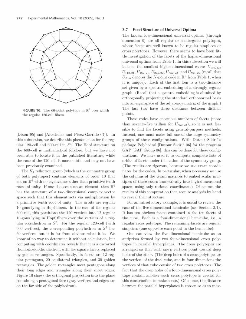
FIGURE 10. The 60-point polytope in R3 over which
the regular 120-cell fibers.
[Dixon 95] and [Altschuler and Perez-Garrido 07]). Inthis subsection, we describe this phenomenon for the reg-ular 120-cell and 600-cell in S3. The Hopf structure onthe 600-cell is mathematical folklore, but we have notbeen able to locate it in the published literature, whilethe case of the 120-cell is more subtle and may not havebeen previously examined.
The H4 reflection group (which is the symmetry groupof both polytopes) contains elements of order 10 thatact on R4 with no eigenvalues other than primitive tenthroots of unity. If one chooses such an element, then R
4
has the structure of a two-dimensional complex vectorspace such that this element acts via multiplication bya primitive tenth root of unity. The orbits are regular10-gons lying in Hopf fibers. In the case of the regular600-cell, this partitions the 120 vertices into 12 regular10-gons lying in Hopf fibers over the vertices of a reg-ular icosahedron in S2. For the regular 120-cell (with600 vertices), the corresponding polyhedron in S2 has60 vertices, but it is far from obvious what it is. Weknow of no way to determine it without calculation, butcomputing with coordinates reveals that it is a distortedrhombicosidodecahedron, with the square facets replacedby golden rectangles. Specifically, its facets are 12 reg-ular pentagons, 20 equilateral triangles, and 30 goldenrectangles. The golden rectangles meet pentagons alongtheir long edges and triangles along their short edges.Figure 10 shows the orthogonal projection into the planecontaining a pentagonal face (gray vertices and edges areon the far side of the polyhedron).
3.7 Facet Structure of Universal OptimaThe known low-dimensional universal optima (throughdimension 8) are all regular or semiregular polytopes,whose facets are well known to be regular simplices orcross polytopes. However, there seems to have been lit-tle investigation of the facets of the higher-dimensionaluniversal optima from Table 1. In this subsection we willlook at the smallest higher-dimensional cases: U100,22,U112,21, U162,21, U275,22, U552,23, and U891,22 (recall thatUN,n denotes the N -point code in Rn from Table 1, whenit is unique). Each of the first four is a two-distanceset given by a spectral embedding of a strongly regulargraph. (Recall that a spectral embedding is obtained byorthogonally projecting the standard orthonormal basisinto an eigenspace of the adjacency matrix of the graph.)The last two have three distances between distinctpoints.
These codes have enormous numbers of facets (morethan seventy-five trillion for U552,23), so it is not fea-sible to find the facets using general-purpose methods.Instead, one must make full use of the large symmetrygroups of these configurations. With Dutour Sikiric’spackage Polyhedral [Dutour Sikiric 06] for the programGAP [GAP Group 06], this can be done for these config-urations. We have used it to compute complete lists oforbits of facets under the action of the symmetry group.(The results are rigorous, because we use exact coordi-nates for the codes. In particular, when necessary we usethe columns of the Gram matrices to embed scalar mul-tiples of these codes isometrically into high-dimensionalspaces using only rational coordinates.) Of course, theresults of this computation then require analysis by handto reveal their structure.
For an introductory example, it is useful to review thecase of the five-dimensional hemicube (see Section 3.1).It has ten obvious facets contained in the ten facets ofthe cube. Each is a four-dimensional hemicube, i.e., aregular cross polytope. The remaining facets are regularsimplices (one opposite each point in the hemicube).
One can view the five-dimensional hemicube as anantiprism formed by two four-dimensional cross poly-topes in parallel hyperplanes. The cross polytopes arearranged so that each one’s vertices point toward deepholes of the other. (The deep holes of a cross polytope arethe vertices of the dual cube, and in four dimensions thevertices of that cube consist of two cross polytopes. Thefact that the deep holes of a four-dimensional cross poly-tope contain another such cross polytope is crucial forthis construction to make sense.) Of course, the distancebetween the parallel hyperplanes is chosen so as to max-
Ballinger et al.: Experimental Study of Energy-Minimizing Point Configurations on Spheres 273
imize the minimal distance. What is remarkable aboutthis antiprism is that it is far more symmetrical than onemight expect: normally the two starting facets of an an-tiprism play a very different role from the facets formedby taking the convex hull, but in this case extra symme-tries occur. The simplest case of such extra symmetriesis the construction of a cross polytope as an antiprismmade from two regular simplices in dual position.
The three universal optima U100,22, U112,21, andU162,21 are each given by an unusually symmetric an-tiprism construction analogous to that of the hemicube.In each case, the largest facets (i.e., those containing themost vertices) contain half the vertices. These facetsare themselves spectral embeddings of strongly regu-lar graphs (the Hoffman–Singleton graph, the Gewirtzgraph, and the unique (81, 20, 1, 6) strongly regulargraph). Within the universal optima, the largest facetsoccur in pairs in parallel hyperplanes, and the verticesof each facet in a pair point toward holes in the other.These holes belong to a single orbit under the symmetrygroup of the facet, and that orbit is the disjoint unionof several copies of the vertices of the facet: two copiesfor the Hoffman–Singleton and Gewirtz cases and four inthe third case. These holes are the deepest holes in theHoffman–Singleton case; in the other two cases, they arenot quite the deepest holes (there are not enough deepholes for the construction to work using them).
Brouwer and Haemers [Brouwer and Haemers 92,Brouwer and Haemers 93] discovered the underlying com-binatorics of these constructions (i.e., that the stronglyregular graphs corresponding to the universal optima canbe naturally partitioned into two identical graphs). How-ever, the geometric interpretation as antiprisms appearsto be new.
The universal optima U100,22, U112,21, and U162,21 areantiprisms, but that cannot possibly be true for U275,22,because 275 is odd. Instead, the McLaughlin config-uration U275,22 is analogous to the Schlafli configura-tion U27,6. Both are two-distance sets. In the Schlafliconfiguration, the neighbors of each point form a five-dimensional hemicube and the nonneighbors form a five-dimensional cross polytope. Both the hemicube and thecross polytope are unusually symmetric antiprisms, andtheir vertices point toward each other’s deep holes. (Thedeep holes of the hemicube form a cross polytope, andthose of the cross polytope form a cube consisting of twohemicubes.) The McLaughlin configuration is completelyanalogous: the neighbors of each point form U162,21 andthe nonneighbors form U112,21. They point toward eachother’s deep holes; this is possible because the deep holes
of U112,21 consist of four copies of U162,21, and its deepholes consist of two copies of U112,21. Furthermore, thedeep holes in these two universal optima are of exactlythe same depth (i.e., distance to the nearest point in thecode), as is also the case for the five-dimensional crosspolytope and hemicube used to form the Schlafli config-uration.
The Schlafli and McLaughlin configurations both havethe property that their deep holes are the antipodes oftheir vertices. Thus, it is natural to form antiprisms fromtwo parallel copies of them, with vertices pointed at eachother’s deep holes. That yields antipodal configurationsof 54 points in R
7 and 550 points in R23. If one also
includes the two points orthogonal to the parallel hyper-planes containing the original two copies, then this con-struction gives the universal optima U56,7 and U552,23.
Each high-dimensional universal optimum has manytypes of facets of different sizes. For example, the facetsof the Higman–Sims configuration U100,22 form 123 or-bits under the action of the symmetry group (see Ta-ble 9). The largest facets, which come from the Hoffman–Singleton graph as described above, are by far the mostimportant, but each type of facet appears to be of inter-est. They are often more subtle than one might expect.For example, it is natural to guess that the facets with42 vertices would be regular cross polytopes, based onthe number of vertices, but they are not. Instead, whenrescaled to the unit sphere they have the following struc-ture:
The facets with 42 vertices are two-distance sets onthe unit sphere in R
21, with inner products 1/29 and−13/29. If we define a graph on the vertices by lettingedges correspond to pairs with inner product −13/29,then this graph is the bipartite incidence graph for pointsand lines in the projective plane P2(F4). To embed thisgraph in R21, represent the 21 points in P2(F4) as thepermutations of (a, b, . . . , b), where a2 + 20b2 = 1 and2ab + 19b2 = 1/29. Specifically, take a = 0.9977 . . . andb = 0.0151 . . . (these are fourth-degree algebraic num-bers). Choose c and d so that 5c2 + 16d2 = 1 and8cd+ c2 +12d2 = 1/29 (specifically, take c = −0.4362 . . .
and d = 0.0550 . . . ). Then embed the 21 lines into R21 aspermutations of (c, c, c, c, c, d, . . . , d), where the five c en-tries correspond to the points contained in the line. Thisembedding gives the inner products of 1/29 and −13/29,as desired (and in fact those are the only inner productsfor which a construction of this form is possible).
As shown in Table 9, there are 92 different types ofsimplicial facets in the Higman–Sims configuration. Oneorbit consists of regular simplices: for each point in the
274 Experimental Mathematics, Vol. 18 (2009), No. 3
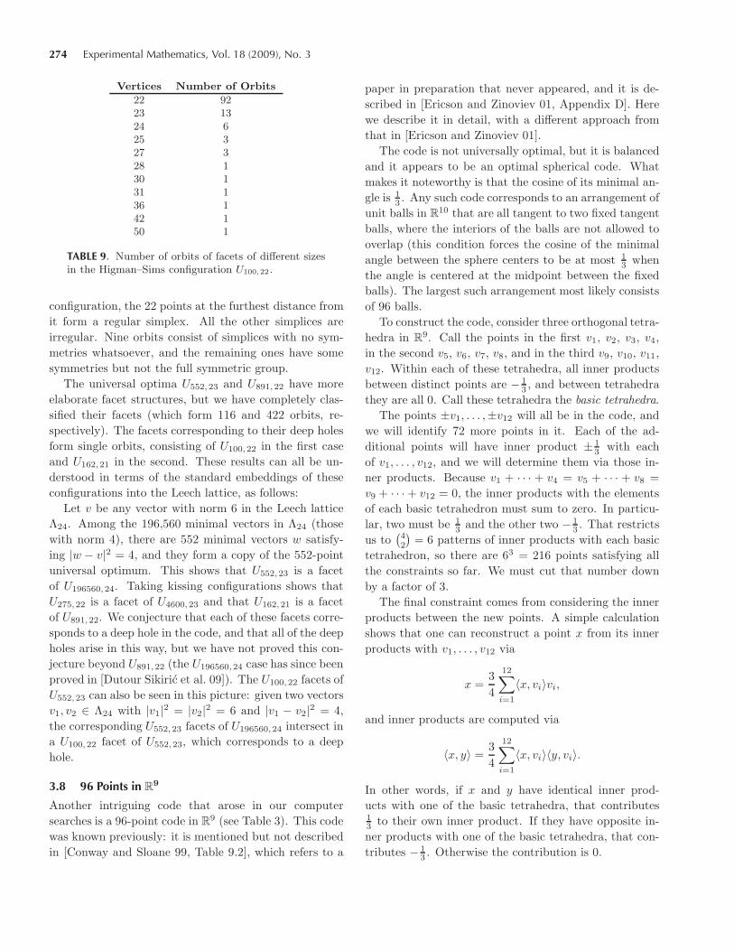
Vertices Number of Orbits
22 9223 1324 625 327 328 130 131 136 142 150 1
TABLE 9. Number of orbits of facets of different sizesin the Higman–Sims configuration U100,22 .
configuration, the 22 points at the furthest distance fromit form a regular simplex. All the other simplices areirregular. Nine orbits consist of simplices with no sym-metries whatsoever, and the remaining ones have somesymmetries but not the full symmetric group.
The universal optima U552,23 and U891,22 have moreelaborate facet structures, but we have completely clas-sified their facets (which form 116 and 422 orbits, re-spectively). The facets corresponding to their deep holesform single orbits, consisting of U100,22 in the first caseand U162,21 in the second. These results can all be un-derstood in terms of the standard embeddings of theseconfigurations into the Leech lattice, as follows:
Let v be any vector with norm 6 in the Leech latticeΛ24. Among the 196,560 minimal vectors in Λ24 (thosewith norm 4), there are 552 minimal vectors w satisfy-ing |w − v|2 = 4, and they form a copy of the 552-pointuniversal optimum. This shows that U552,23 is a facetof U196560,24. Taking kissing configurations shows thatU275,22 is a facet of U4600,23 and that U162,21 is a facetof U891,22. We conjecture that each of these facets corre-sponds to a deep hole in the code, and that all of the deepholes arise in this way, but we have not proved this con-jecture beyond U891,22 (the U196560,24 case has since beenproved in [Dutour Sikiric et al. 09]). The U100,22 facets ofU552,23 can also be seen in this picture: given two vectorsv1, v2 ∈ Λ24 with |v1|2 = |v2|2 = 6 and |v1 − v2|2 = 4,the corresponding U552,23 facets of U196560,24 intersect ina U100,22 facet of U552,23, which corresponds to a deephole.
3.8 96 Points in R9
Another intriguing code that arose in our computersearches is a 96-point code in R9 (see Table 3). This codewas known previously: it is mentioned but not describedin [Conway and Sloane 99, Table 9.2], which refers to a
paper in preparation that never appeared, and it is de-scribed in [Ericson and Zinoviev 01, Appendix D]. Herewe describe it in detail, with a different approach fromthat in [Ericson and Zinoviev 01].
The code is not universally optimal, but it is balancedand it appears to be an optimal spherical code. Whatmakes it noteworthy is that the cosine of its minimal an-gle is 1
3 . Any such code corresponds to an arrangement ofunit balls in R10 that are all tangent to two fixed tangentballs, where the interiors of the balls are not allowed tooverlap (this condition forces the cosine of the minimalangle between the sphere centers to be at most 1
3 whenthe angle is centered at the midpoint between the fixedballs). The largest such arrangement most likely consistsof 96 balls.
To construct the code, consider three orthogonal tetra-hedra in R9. Call the points in the first v1, v2, v3, v4,in the second v5, v6, v7, v8, and in the third v9, v10, v11,v12. Within each of these tetrahedra, all inner productsbetween distinct points are − 1
3 , and between tetrahedrathey are all 0. Call these tetrahedra the basic tetrahedra.
The points ±v1, . . . ,±v12 will all be in the code, andwe will identify 72 more points in it. Each of the ad-ditional points will have inner product ± 1
3 with eachof v1, . . . , v12, and we will determine them via those in-ner products. Because v1 + · · · + v4 = v5 + · · · + v8 =v9 + · · · + v12 = 0, the inner products with the elementsof each basic tetrahedron must sum to zero. In particu-lar, two must be 1
3 and the other two − 13 . That restricts
us to(42
)= 6 patterns of inner products with each basic
tetrahedron, so there are 63 = 216 points satisfying allthe constraints so far. We must cut that number downby a factor of 3.
The final constraint comes from considering the innerproducts between the new points. A simple calculationshows that one can reconstruct a point x from its innerproducts with v1, . . . , v12 via
x =34
12∑i=1
〈x, vi〉vi,
and inner products are computed via
〈x, y〉 =34
12∑i=1
〈x, vi〉〈y, vi〉.
In other words, if x and y have identical inner prod-ucts with one of the basic tetrahedra, that contributes13 to their own inner product. If they have opposite in-ner products with one of the basic tetrahedra, that con-tributes − 1
3 . Otherwise the contribution is 0.
Ballinger et al.: Experimental Study of Energy-Minimizing Point Configurations on Spheres 275
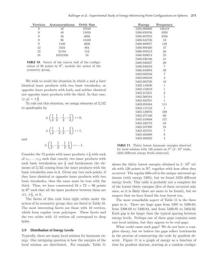
Vertices Automorphisms Orbit Size
9 16 276489 48 138249 48 46089 96 184329 1440 460812 1024 86412 31104 51216 10321920 18
TABLE 10. Facets of the convex hull of the configu-ration of 96 points in R
9, modulo the action of thesymmetry group.
We wish to avoid the situation in which x and y haveidentical inner products with two basic tetrahedra, oropposite inner products with both, and neither identicalnor opposite inner products with the third. In that case,〈x, y〉 = ± 2
3 .To rule out this situation, we assign elements of Z/3Z
to quadruples by
±(
13,13,−1
3,−1
3
)→ 0,
±(
13,−1
3,13,−1
3
)→ 1,
and
±(
13,−1
3,−1
3,13
)→ −1.
Consider the 72 points with inner products ± 13 with each
of v1, . . . , v12 such that exactly two inner products witheach basic tetrahedron are 1
3 and furthermore the ele-ments of Z/3Z coming from the inner products with thebasic tetrahedra sum to 0. Given any two such points, ifthey have identical or opposite inner products with twobasic tetrahedra, then the same must be true with thethird. Thus, we have constructed 24 + 72 = 96 pointsin R
9 such that all the inner products between them are±1, ± 1
3 , or 0.The facets of this code form eight orbits under the
action of its symmetry group; they are listed in Table 10.The most interesting facets are those with 16 vertices,which form regular cross polytopes. These facets andthe two orbits with 12 vertices all correspond to deepholes.
3.9 Distribution of Energy Levels
Typically, there are many local minima for harmonic en-ergy. One intriguing question is how the energies of thelocal minima are distributed. For example, Table 11
Energy Frequency
5395.000000 1864185398.650556 43935398.687876 23565400.842726 185400.880057 1495400.890460 475400.894513 265400.928674 255400.936106 415400.940237 285400.940550 75400.943094 385402.029556 75402.088248 35402.093726 105402.116636 15402.152619 15402.213231 25402.366164 15402.922701 15403.091064 1115403.115123 15403.129076 1085403.271100 665403.319898 1575403.326719 845403.347209 245403.455701 75403.462898 85403.488923 4
TABLE 11. Thirty lowest harmonic energies observedfor local minima with 120 points on S3 (2 · 105 trials,5223 different energy levels observed).
shows the thirty lowest energies obtained in 2 · 105 tri-als with 120 points in R4, together with how often theyoccurred. The regular 600-cell is the unique universal op-timum (with energy 5395), but we found 5223 differentenergy levels. This table is probably not a complete listof the lowest thirty energies (five of them occurred onlyonce, so it is likely there are more to be found), but wesuspect that we have found the true lowest ten.
The most remarkable aspect of Table 11 is the threegaps in it. There are huge gaps from 5395 to 5398.65,from 5398.69 to 5400.84, and from 5400.95 to 5402.02.Each gap is far larger than the typical spacing betweenenergy levels. Perhaps one of these gaps contains somerare local minima, but they appear to be real gaps.
What could cause such gaps? We do not have a com-plete theory, but we believe the gaps reflect bottlenecksin the process of constructing the code by gradient de-scent. Figure 11 is a graph of energy as a function oftime for gradient descent, starting at a random configu-
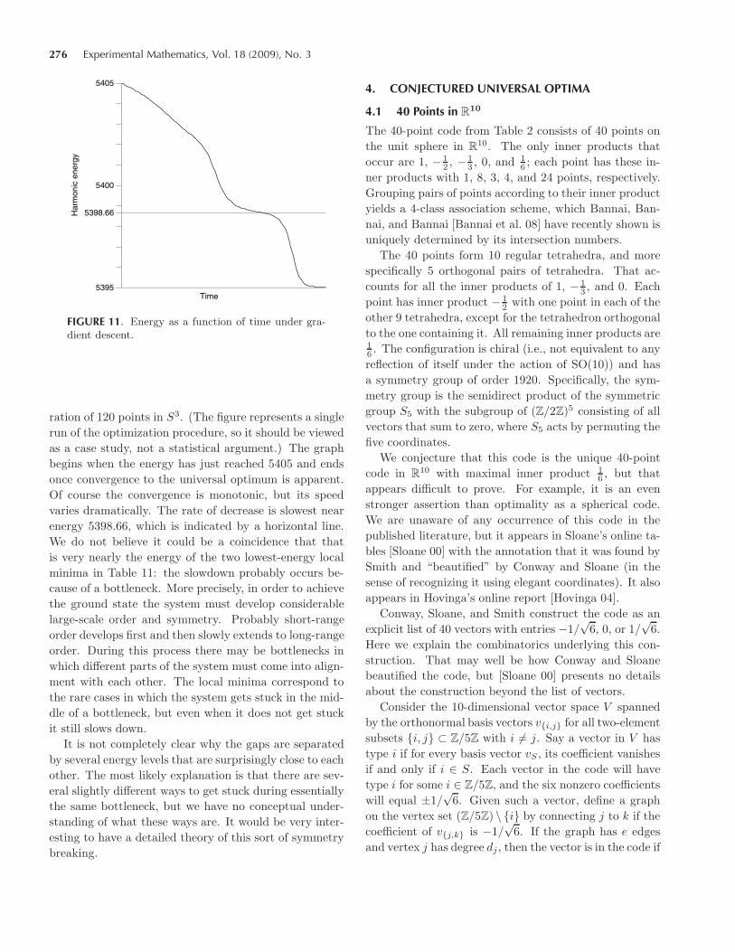
276 Experimental Mathematics, Vol. 18 (2009), No. 3
Time
Har
mon
ic e
nerg
y
5395
5400
5405
5398.66
FIGURE 11. Energy as a function of time under gra-dient descent.
ration of 120 points in S3. (The figure represents a singlerun of the optimization procedure, so it should be viewedas a case study, not a statistical argument.) The graphbegins when the energy has just reached 5405 and endsonce convergence to the universal optimum is apparent.Of course the convergence is monotonic, but its speedvaries dramatically. The rate of decrease is slowest nearenergy 5398.66, which is indicated by a horizontal line.We do not believe it could be a coincidence that thatis very nearly the energy of the two lowest-energy localminima in Table 11: the slowdown probably occurs be-cause of a bottleneck. More precisely, in order to achievethe ground state the system must develop considerablelarge-scale order and symmetry. Probably short-rangeorder develops first and then slowly extends to long-rangeorder. During this process there may be bottlenecks inwhich different parts of the system must come into align-ment with each other. The local minima correspond tothe rare cases in which the system gets stuck in the mid-dle of a bottleneck, but even when it does not get stuckit still slows down.
It is not completely clear why the gaps are separatedby several energy levels that are surprisingly close to eachother. The most likely explanation is that there are sev-eral slightly different ways to get stuck during essentiallythe same bottleneck, but we have no conceptual under-standing of what these ways are. It would be very inter-esting to have a detailed theory of this sort of symmetrybreaking.
4. CONJECTURED UNIVERSAL OPTIMA
4.1 40 Points in R10
The 40-point code from Table 2 consists of 40 points onthe unit sphere in R10. The only inner products thatoccur are 1, − 1
2 , − 13 , 0, and 1
6 ; each point has these in-ner products with 1, 8, 3, 4, and 24 points, respectively.Grouping pairs of points according to their inner productyields a 4-class association scheme, which Bannai, Ban-nai, and Bannai [Bannai et al. 08] have recently shown isuniquely determined by its intersection numbers.
The 40 points form 10 regular tetrahedra, and morespecifically 5 orthogonal pairs of tetrahedra. That ac-counts for all the inner products of 1, − 1
3 , and 0. Eachpoint has inner product − 1
2 with one point in each of theother 9 tetrahedra, except for the tetrahedron orthogonalto the one containing it. All remaining inner products are16 . The configuration is chiral (i.e., not equivalent to anyreflection of itself under the action of SO(10)) and hasa symmetry group of order 1920. Specifically, the sym-metry group is the semidirect product of the symmetricgroup S5 with the subgroup of (Z/2Z)5 consisting of allvectors that sum to zero, where S5 acts by permuting thefive coordinates.
We conjecture that this code is the unique 40-pointcode in R10 with maximal inner product 1
6 , but thatappears difficult to prove. For example, it is an evenstronger assertion than optimality as a spherical code.We are unaware of any occurrence of this code in thepublished literature, but it appears in Sloane’s online ta-bles [Sloane 00] with the annotation that it was found bySmith and “beautified” by Conway and Sloane (in thesense of recognizing it using elegant coordinates). It alsoappears in Hovinga’s online report [Hovinga 04].
Conway, Sloane, and Smith construct the code as anexplicit list of 40 vectors with entries −1/
√6, 0, or 1/
√6.
Here we explain the combinatorics underlying this con-struction. That may well be how Conway and Sloanebeautified the code, but [Sloane 00] presents no detailsabout the construction beyond the list of vectors.
Consider the 10-dimensional vector space V spannedby the orthonormal basis vectors v{i,j} for all two-elementsubsets {i, j} ⊂ Z/5Z with i �= j. Say a vector in V hastype i if for every basis vector vS , its coefficient vanishesif and only if i ∈ S. Each vector in the code will havetype i for some i ∈ Z/5Z, and the six nonzero coefficientswill equal ±1/
√6. Given such a vector, define a graph
on the vertex set (Z/5Z) \ {i} by connecting j to k if thecoefficient of v{j,k} is −1/
√6. If the graph has e edges
and vertex j has degree dj , then the vector is in the code if
Ballinger et al.: Experimental Study of Energy-Minimizing Point Configurations on Spheres 277
and only if di+1 ≡ di+2 ≡ e (mod 2) and di−1 ≡ di−2 �≡ e
(mod 2) (where i is the type of the vector).The facet structure of this code seems surprisingly
unilluminating compared to the others we have analyzed.There are 24 orbits of facets: 21 orbits of irregular sim-plices (with symmetry groups ranging from 2 to 768 insize), one orbit of 11-vertex facets, and two orbits of 12-vertex facets. The most symmetrical facets are thosein one of the two orbits of 12-vertex facets. They have3072 symmetries and are given by the orthogonal unionof three identical irregular tetrahedra in R3 (with eightsymmetries).
Our confidence in this code’s universal optimality isbased on detailed numerical experiments. One reason aconfiguration could be universally optimal is that it hasno competitors (i.e., except in degenerate cases there areno other local minima). That is not true for the 40-pointcode, but there are remarkably few competitors. In par-ticular, it appears to have only one “serious” competitor.We have found five other families of local minima, butfour of them are rare and never seem to come close tobeating our conjectured universal optimum. The bestexperimental evidence we can imagine for universal op-timality would be to describe explicitly each competingfamily that has been observed and prove that it nevercontains the global energy minimum. That might be pos-sible for this code, but we have not completed it. The fourrare families are sufficiently complicated that we have notanalyzed them explicitly (under the circumstances it didnot seem worth the effort). However, we have a completedescription of the serious competitor.
That family depends on a parameter α that must sat-isfy 0 < α2 ≤ 1/27. The configuration always contains afixed 16-point subset with the following structure. If wecall the 16 points wi,j with i, j ∈ {1, 2, 3, 4}, then
〈wi,j , wk,�〉 =
⎧⎪⎨⎪⎩
1 if (i, j) = (k, �),− 1
3 if i = k or j = � but not both, and19 otherwise.
In other words, if we arrange the points in a 4 × 4 grid,then the rows and columns are regular tetrahedra and allother inner products are 1
9 . To construct such a configu-ration, take the tensor product in R3 ⊗R R3 = R9 of tworegular tetrahedra in R
3.To describe the remaining 24 points, we will specify
their inner products with the first 16 points. That willdetermine their projections into the 9-dimensional sub-space containing the 16 points, so the only additional in-formation needed to pin them down will be whether they
are above or below that hyperplane (relative to some ori-entation).
Each of the 24 points will have inner product −3α
with four of the first 16 points and α with each of theothers. The only constraint is that it must have innerproduct −3α with exactly four points, one in each ofthe eight tetrahedra (i.e., one in each row and columnof the 4 × 4 grid). The 4 × 4 grid exhibits a one-to-one correspondence with permutations of four elements,so there are 4! = 24 ways to satisfy these constraints.The points corresponding to even permutations will beplaced above the 9-dimensional hyperplane, and thosecorresponding to odd permutations will be placed belowit. This construction yields a 40-point code in R
10 pro-vided that 0 < α2 ≤ 1/27. (When α = 0 some pointscoincide, and when α2 > 1/27 the inner products cannotbe achieved by unit vectors.)
We have not proved that the codes in this family neverimprove on the conjectured universal optimum, but weare confident that it is true. The best spherical code inthe family occurs when α = (
√109− 1)/54 = 0.1748 . . . ;
in this special case, α is also the maximal inner product,which is quite a bit larger than the maximal inner prod-uct 1
6 in the conjectured universal optimum. That impliesthat when k is sufficiently large, the conjectured opti-mum is better for the potential function f(r) = (4 − r)k
(because the energy is dominated asymptotically by thecontribution from the minimal distance). In principle onecould verify the finitely many remaining values of k by afinite computation. We have done enough exploration toconvince ourselves that it is true, but we have not founda rigorous proof.
4.2 64 Points in R14
The simplest construction we are aware of for the 64-point configuration in R14 uses the Nordstrom–Robinsonbinary code [Nordstrom and Robinson 67, Griess 08].Shortening that code twice yields a binary code of length14, size 64, and minimal distance 6, which is known tobe unique [MacWilliams and Sloane 77, pp. 74–75]. Onecan view it as a subset of the cube {−1, 1}14 instead of{0, 1}14. Then after rescaling by a factor of 1/
√14 to
yield unit vectors, this code is the 64-point configurationin R14 that we conjecture is universally optimal. Thesame process with less shortening yields the codes fromTables 3 and 4 with 128 points in R
15 and 256 pointsin R16; the 64-point and 128-point codes have previouslyappeared in [Ericson and Zinoviev 01, Appendix D] viathe same approach, as conjectures for optimal sphericalcodes.
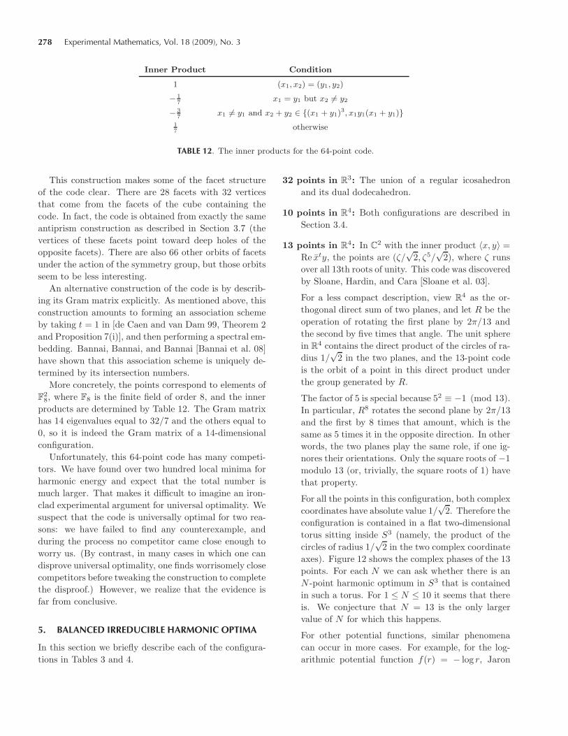
278 Experimental Mathematics, Vol. 18 (2009), No. 3
Inner Product Condition
1 (x1, x2) = (y1, y2)
− 17
x1 = y1 but x2 �= y2
− 37
x1 �= y1 and x2 + y2 ∈ {(x1 + y1)3, x1y1(x1 + y1)}
17
otherwise
TABLE 12. The inner products for the 64-point code.
This construction makes some of the facet structureof the code clear. There are 28 facets with 32 verticesthat come from the facets of the cube containing thecode. In fact, the code is obtained from exactly the sameantiprism construction as described in Section 3.7 (thevertices of these facets point toward deep holes of theopposite facets). There are also 66 other orbits of facetsunder the action of the symmetry group, but those orbitsseem to be less interesting.
An alternative construction of the code is by describ-ing its Gram matrix explicitly. As mentioned above, thisconstruction amounts to forming an association schemeby taking t = 1 in [de Caen and van Dam 99, Theorem 2and Proposition 7(i)], and then performing a spectral em-bedding. Bannai, Bannai, and Bannai [Bannai et al. 08]have shown that this association scheme is uniquely de-termined by its intersection numbers.
More concretely, the points correspond to elements ofF
28, where F8 is the finite field of order 8, and the inner
products are determined by Table 12. The Gram matrixhas 14 eigenvalues equal to 32/7 and the others equal to0, so it is indeed the Gram matrix of a 14-dimensionalconfiguration.
Unfortunately, this 64-point code has many competi-tors. We have found over two hundred local minima forharmonic energy and expect that the total number ismuch larger. That makes it difficult to imagine an iron-clad experimental argument for universal optimality. Wesuspect that the code is universally optimal for two rea-sons: we have failed to find any counterexample, andduring the process no competitor came close enough toworry us. (By contrast, in many cases in which one candisprove universal optimality, one finds worrisomely closecompetitors before tweaking the construction to completethe disproof.) However, we realize that the evidence isfar from conclusive.
5. BALANCED IRREDUCIBLE HARMONIC OPTIMA
In this section we briefly describe each of the configura-tions in Tables 3 and 4.
32 points in R3: The union of a regular icosahedron
and its dual dodecahedron.
10 points in R4: Both configurations are described inSection 3.4.
13 points in R4: In C
2 with the inner product 〈x, y〉 =Re xty, the points are (ζ/
√2, ζ5/
√2), where ζ runs
over all 13th roots of unity. This code was discoveredby Sloane, Hardin, and Cara [Sloane et al. 03].
For a less compact description, view R4 as the or-thogonal direct sum of two planes, and let R be theoperation of rotating the first plane by 2π/13 andthe second by five times that angle. The unit spherein R4 contains the direct product of the circles of ra-dius 1/
√2 in the two planes, and the 13-point code
is the orbit of a point in this direct product underthe group generated by R.
The factor of 5 is special because 52 ≡ −1 (mod 13).In particular, R8 rotates the second plane by 2π/13and the first by 8 times that amount, which is thesame as 5 times it in the opposite direction. In otherwords, the two planes play the same role, if one ig-nores their orientations. Only the square roots of −1modulo 13 (or, trivially, the square roots of 1) havethat property.
For all the points in this configuration, both complexcoordinates have absolute value 1/
√2. Therefore the
configuration is contained in a flat two-dimensionaltorus sitting inside S3 (namely, the product of thecircles of radius 1/
√2 in the two complex coordinate
axes). Figure 12 shows the complex phases of the 13points. For each N we can ask whether there is anN -point harmonic optimum in S3 that is containedin such a torus. For 1 ≤ N ≤ 10 it seems that thereis. We conjecture that N = 13 is the only largervalue of N for which this happens.
For other potential functions, similar phenomenacan occur in more cases. For example, for the log-arithmic potential function f(r) = − log r, Jaron
Ballinger et al.: Experimental Study of Energy-Minimizing Point Configurations on Spheres 279
FIGURE 12. The 13-point harmonic optimum in S3,drawn on a torus by plotting (φ, ψ) for the point(eiφ/
√2, eiψ/
√2).
Lanier has conjectured in a private communicationthat the minimal-energy configuration of 11 pointson S3 also lies on a flat torus. In C2, the points are(αζ,
√1 − α2ζ4), where ζ runs over all 11th roots of
unity and α is the unique root between 0 and 1 of
5α8 − 36α6 + 51α4 − 4α2 − 7 = 0.
15 points in R4: Described in Section 3.1.
24 points in R4: The regular 24-cell (equivalently, theD4 root system).
48 points in R4: Described in Section 3.5.
21 points in R5: The edge midpoints and face centersof a regular simplex (rescaled to lie on the samesphere).
32 points in R5: Start with a regular simplex v1, . . . , v6
in R5. The 32 points will be these six points andtheir negatives, along with 20 points determinedas follows by their inner products with v1, . . . , v6.Each will have inner product ±1/
√5 with each of
v1, . . . , v6, with three plus signs and three minussigns. There are
(63
)= 20 ways to choose these signs.
2n + 2 points in Rn (for n ≥ 6): Described in Sec-tion 3.4.
42 points in R6: The edge midpoints of a regular sim-plex and their antipodes.
44 points in R6: This code contains plus or minus an
orthonormal basis of R6 together with the 32 vec-tors whose coordinates with respect to that basisare ±1/
√6 and where the number of minus signs is
even. It other words, it consists of a cross polytopeand a hemicube within the cube dual to the crosspolytope. This code was previously conjectured tobe an optimal spherical code (see [Ericson and Zi-noviev 01, Table D.6]).
126 points in R6: The union of the minimal vectors of
the E6 and E∗6 lattices (rescaled to lie on the same
sphere). Equivalently, one can project the E7 rootsystem orthogonally to a minimal vector in E∗
7 , fol-lowed by rescaling as in the first construction.
78 points in R7: Like the 44 points in R
6, this codeconsists of a cross polytope and a hemicube withinthe cube dual to the cross polytope.
148 points in R7: The points are all the permutationsof
(±1,±1, 0, 0, 0, 0, 0)√2
and the hemicube consisting of the points
(±1,±1,±1,±1,±1,±1,±1)√7
that have an even number of minus signs. This is aseven-dimensional analogue of a construction of theE8 root system, but it is less symmetric, becausethe two types of points form distinct orbits underthe action of the symmetry group. This code waspreviously conjectured to be an optimal sphericalcode (see [Ericson and Zinoviev 01, Table D.7]).
182 points in R7: The union of the minimal vectors ofthe E7 and E∗
7 lattices (rescaled to lie on the samesphere). Equivalently, one can project the E8 rootsystem orthogonally to any root; 126 roots are un-changed, 112 project to 56 nonzero points, and 2project to the origin. Rescaling the nonzero projec-tions to lie on the unit sphere yields the 182-pointconfiguration.
72 points in R8: The edge midpoints of a regular sim-
plex and their antipodes. This code was previouslyconjectured to be an optimal spherical code (see [Er-icson and Zinoviev 01, Table D.8]).
96 points in R9: Described in Section 3.8.
280 Experimental Mathematics, Vol. 18 (2009), No. 3
42 points in R14: This code consists of seven disjointfive-dimensional regular simplices, whose verticeshave inner products − 1
5 with each other. Each pointhas inner product − 1
2 with a unique point in eachsimplex other than the one containing it, and allother inner products between points in different sim-plices are 1
10 . Grouping pairs of points accordingto their inner product yields a three-class associa-tion scheme that can be derived from the Hoffman–Singleton graph (see [van Dam 99, Section 5.1]). LetG be the Hoffman–Singleton graph, and let H beits second subconstituent. In other words, take anyvertex v in G, and let H be the vertices not equalto or adjacent to v. The vertices in H correspondto points in the 14-dimensional configuration, withinner product − 1
2 between adjacent vertices, − 15 be-
tween nonadjacent vertices with no common neigh-bor, and 1
10 between nonadjacent vertices with onecommon neighbor. This code was previously conjec-tured to be an optimal spherical code (see [Ericsonand Zinoviev 01, Table D.14]).
128 points in R15: Described in Section 4.2.
256 points in R16: Described in Section 4.2.
6. CHALLENGES
We conclude with a list of computational and theoreticalchallenges:
1. How often do 196,560 randomly chosen points on S23
converge to the Leech lattice minimal vectors un-der gradient descent for harmonic energy? For 240points on S7, one frequently obtains the E8 root sys-tem (855 times out of 1000 trials), and the Higman–Sims configuration of 100 points on S21 occurs fairlyoften (257 times out of 1000 trials); by contrast, theuniversal optimum with 112 points on S20 occursrarely (once in 1000 trials). This approach could bean intriguing construction of the Leech lattice, butwe have no intuition for how likely it is to work.
2. What are the potential energy barriers that sepa-rate the local minima in Table 5 (or any other case)?In other words, if one continuously transforms oneconfiguration into another, how low can one makethe greatest energy along the path connecting them?The lowest possible point of greatest energy will al-ways be a saddle point for the energy function.
3. How many harmonic local minima are there for 120points on S3 (Table 11), or even 64 points on S13? Isthe number small enough that one could conceivablycompile a complete list? Is the list for 27 points onS5 in Table 5 complete?
4. For large numbers of points, what can one say (ex-perimentally, heuristically, or rigorously) about thedistribution of energy levels for local minima, orabout the gaps in the distribution?
7. APPENDIX: LOCAL NONOPTIMALITYOF DIPLO-SIMPLICES
In this appendix we prove that (above dimension two)diplo-simplices are not even locally optimal as sphericalcodes. The motivation behind the calculations is the caseof n = 3, where the diplo-simplex is a cube. One can im-prove this spherical code by rotating one face relativeto the opposite face while moving them slightly closertogether. To carry out this approach in higher dimen-sions, we must understand the faces of the diplo-simplex(which is in general quite different from the hypercube).The diplo-simplex in R
n is the orthogonal projection ofthe vertices of the cross polytope in Rn+1 onto the hy-perplane on which the sum of the coordinates is zero.Its dual polytope is therefore the cross section of the hy-percube in Rn+1 by that hyperplane. The vertices ofthe cross section differ depending on whether n is odd oreven: (1, . . . , 1,−1, . . . ,−1) is a vertex when n+1 is even,and (1, . . . , 1, 0,−1, . . . ,−1) is when n + 1 is odd. Thatleads to the following description of the diplo-simplex,based on identifying its faces using this correspondence.
Let v1, . . . , vk and w1, . . . , wk be unit vectors formingtwo orthogonal (k−1)-dimensional regular simplices, andlet t be a unit vector orthogonal to both simplices. The(2k − 1)-dimensional diplo-simplex consists of the points
±(αvi +
√1 − α2t
)
and±
(αwi +
√1 − α2t
),
where α =√
(2k − 2)/(2k − 1). To improve its minimalangle, use the points
αvi +√
1 − α2t,
αwi +√
1 − α2t,
−(α
(βvi +
√1 − β2wi
)+
√1 − α2t
),
−(α
(√1 − β2vi − βwi
)+
√1 − α2t
),
Ballinger et al.: Experimental Study of Energy-Minimizing Point Configurations on Spheres 281
with β a small positive number and α slightly greaterthan
√(2k − 2)/(2k − 1). When k = 1, choosing α and
β optimally leads to the optimal 8-point code in R3, butwhen k = 3, Sloane’s tables [Sloane 00] show that thisapproach is suboptimal.
The situation is slightly more complicated for even-dimensional diplo-simplices. Again, let v1, . . . , vk andw, . . . , wk be unit vectors forming two orthogonal (k−1)-dimensional simplices. Let t and z be two unit vectorsorthogonal to both simplices and each other. The 2k-dimensional diplo-simplex consists of the points z, −z,
±(αvi + βz +
√1 − α2 − β2t
),
and±
(αwi − βz +
√1 − α2 − β2t
),
where α =√
(2k + 1)(2k − 2)/(2k) and β = 1/(2k).Note that α vanishes when k = 1 and our constructionbelow will not work. Indeed the hexagon, which is thediplo-simplex in the plane, is an optimal spherical code.To improve the minimal angle for k ≥ 2 use the pointsz, −z,
αvi + βz +√
1 − α2 − β2t,
αwi − βz +√
1 − α2 − β2t,
−(α
(γvi +
√1 − γ2wi
)− βz +
√1 − α2 − β2t
),
−(α
(√1 − γ2vi − γwi
)+ βz +
√1 − α2 − β2t
),
with γ a small positive number, α slightly larger than√(2k + 1)(2k − 2)/(2k), and β slightly less than 1/(2k).
The numbers α and β should be chosen such that α2+2β2
increases from its original value of (2k − 1)/(2k).
ACKNOWLEDGMENTS
We thank Eiichi Bannai, Christian Borgs, John Conway,Edwin van Dam, Charles Doran, Noam Elkies, FlorianGaisendrees, Robert Griess, Abhinav Kumar, Jaron Lanier,James Morrow, Frank Stillinger, and Salvatore Torquato forhelpful discussions.
Ballinger and Giansiracusa were supported by the Uni-versity of Washington Mathematics Department’s NSF VI-GRE grant. Schurmann was supported by the DeutscheForschungsgemeinschaft (DFG) under grant SCHU 1503/4-1.
REFERENCES
[Altschuler and Perez-Garrido 05] E. L. Altschuler and A.Perez-Garrido. “Global Minimum for Thomson’s Problemof Charges on a Sphere.” Phys. Rev. E 71 (2005), 047703:1–4.
[Altschuler and Perez-Garrido 06] E. L. Altschuler and A.Perez-Garrido. “Defect Free Global Minima in Thomson’sProblem of Charges on a Sphere.” Phys. Rev. E 73 (2006),036108:1–6.
[Altschuler and Perez-Garrido 07] E. L. Altschuler and A.Perez-Garrido, “Symmetric Four-Dimensional Polytopeand Visualization Method in Four, Eight, and SixteenDimensions Using Hopf Maps.” Phys. Rev. E 76 (2007),016705:1–6.
[Altschuler et al. 97] E. L. Altschuler, T. J. Williams, E.R. Ratner, R. Tipton, R. Stong, F. Dowla, and F.Wooten. “Possible Global Minimum Lattice Configurationsfor Thomson’s Problem of Charges on a Sphere.” Phys.Rev. Lett. 78 (1997), 2681–2685.
[Andreev 96] N. N. Andreev. “An Extremal Property of theIcosahedron.” East J. Approx. 2 (1996), 459–462.
[Andreev 97] N. N. Andreev. “Location of Points on a Spherewith Minimal Energy” (Russian). Tr. Mat. Inst. Steklova219 (1997), 27–31; translation in Proc. Steklov Inst. Math.219 (1997), 20–24.
[Aste and Weaire 08] T. Aste and D. Weaire. The Pursuit ofPerfect Packing , Second edition. New York: Taylor & Fran-cis, 2008.
[Bachoc and Vallentin 09] C. Bachoc and F. Vallentin. “Op-timality and Uniqueness of the (4, 10, 1/6) Spherical Code.”J. Combin. Theory, Ser. A 116 (2009), 195–204.
[Bannai et al. 08] E. Bannai, E. Bannai, and H. Bannai,“Uniqueness of Certain Association Schemes.” European J.Combin. 29 (2008), 1379–1395.
[Bausch et al. 03] A. R. Bausch, M. J. Bowick, A. Cacciuto,A. D. Dinsmore, M. F. Hsu, D. R. Nelson, M. G. Nikolaides,A. Travesset, and D. A. Weitz. “Grain Boundary Scars andSpherical Crystallography.” Science 299 (2003), 1716–1718.
[Boroczky 04] K. Boroczky, Jr. Finite Packing and Covering ,Cambridge Tracts in Mathematics 154. Cambridge: Cam-bridge University Press, 2004.
[Bowick et al. 02] M. Bowick, A. Cacciuto, D. R. Nelson, andA. Travesset. “Crystalline Order on a Sphere and the Gen-eralized Thomson Problem.” Phys. Rev. Lett. 89 (2002),185502:1–4.
[Bowick et al. 06] M. Bowick, A. Cacciuto, D. R. Nelson, andA. Travesset. “Crystalline Particle Packings on a Spherewith Long Range Power Law Potentials.” Phys. Rev. B 73(2006), 024115:1–16.
[Brouwer and Haemers 92] A. E. Brouwer and W. H.Haemers. “Structure and Uniqueness of the (81, 20, 1, 6)Strongly Regular Graph.” Discrete Math. 106/107 (1992),77–82.
[Brouwer and Haemers 93] A. E. Brouwer and W. H.Haemers. “The Gewirtz Graph: An Exercise in the The-ory of Graph Spectra.” European J. Combin. 14 (1993),397–407.
[de Caen and van Dam 99] D. de Caen and E. R. van Dam.“Association Schemes Related to Kasami Codes and Ker-dock Sets.” Des. Codes Cryptogr. 18 (1999), 89–102.
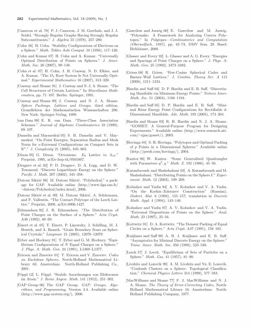
282 Experimental Mathematics, Vol. 18 (2009), No. 3
[Cameron et al. 78] P. J. Cameron, J. M. Goethals, and J. J.Seidel. “Strongly Regular Graphs Having Strongly RegularSubconstituents.” J. Algebra 55 (1978), 257–280.
[Cohn 56] H. Cohn. “Stability Configurations of Electrons ona Sphere.” Math. Tables Aids Comput. 10 (1956), 117–120.
[Cohn and Kumar 07] H. Cohn and A. Kumar. “UniversallyOptimal Distribution of Points on Spheres.” J. Amer.Math. Soc. 20 (2007), 99–148.
[Cohn et al. 07] H. Cohn, J. H. Conway, N. D. Elkies, andA. Kumar. “The D4 Root System Is Not Universally Opti-mal.” Experimental Mathematics 16 (2007), 313–320.
[Conway and Sloane 91] J. Conway and N. J. A. Sloane. “TheCell Structures of Certain Lattices.” In Miscellanea Math-ematica, pp. 71–107. Berlin: Springer, 1991.
[Conway and Sloane 99] J. Conway and N. J. A. Sloane.Sphere Packings, Lattices and Groups, third edition,Grundlehren der Mathematischen Wissenschaften 290.New York: Springer-Verlag, 1999.
[van Dam 99] E. R. van Dam. “Three-Class AssociationSchemes.” Journal of Algebraic Combinatorics 10 (1999),69–107.
[Damelin and Maymeskul 05] S. B. Damelin and V. May-meskul. “On Point Energies, Separation Radius and MeshNorm for s-Extremal Configurations on Compact Sets inR
n.” J. Complexity 21 (2005), 845–863.
[Dixon 95] G. Dixon. “Octonions: E8 Lattice to Λ16.”Preprint, 1995, arXiv:hep-th/9501007.
[Dragnev et al. 02] P. D. Dragnev, D. A. Legg, and D. W.Townsend. “Discrete Logarithmic Energy on the Sphere.”Pacific J. Math. 207 (2002), 345–358.
[Dutour Sikiric 06] M. Dutour Sikiric. “Polyhedral,” a pack-age for GAP. Available online (http://www.liga.ens.fr/∼dutour/Polyhedral/index.html), 2006.
[Dutour Sikiric et al. 09] M. Dutour Sikiric, A. Schurmann,and F. Vallentin. “The Contact Polytope of the Leech Lat-tice.” Preprint, 2009, arXiv:0906.1427.
[Edmundson 92] J. R. Edmundson. “The Distribution ofPoint Charges on the Surface of a Sphere.” Acta Cryst.A48 (1992), 60–69.
[Einert et al. 05] T. Einert, P. Lipowsky, J. Schilling, M. J.Bowick, and A. Bausch. “Grain Boundary Scars on Spher-ical Crystals.” Langmuir 21 (2005), 12076–12079.
[Erber and Hockney 91] T. Erber and G. M. Hockney. “Equi-librium Configurations of N Equal Charges on a Sphere.”J. Phys. A: Math. Gen. 24 (1991), L1369–L1377.
[Ericson and Zinoviev 01] T. Ericson and V. Zinoviev. Codeson Euclidean Spheres, North-Holland Mathematical Li-brary 63. Amsterdam: North-Holland Publishing Co.,2001.
[Foppl 12] L. Foppl. “Stabile Anordnungen von Elektronenim Atom.” J. Reine Angew. Math. 141 (1912), 251–302.
[GAP Group 06] The GAP Group. GAP: Groups, Algo-rithms, and Programming, Version 4.4. Available online(http://www.gap-system.org/), 2006.
[Gawrilow and Joswig 00] E. Gawrilow and M. Joswig.“Polymake: A Framework for Analyzing Convex Poly-topes.” In Polytopes—Combinatorics and Computation(Oberwolfach, 1997), pp. 43–73, DMV Sem. 29. Basel:Birkhauser, 2000.
[Glasser and Every 92] L. Glasser and A. G. Every. “Energiesand Spacings of Point Charges on a Sphere.” J. Phys. A:Math. Gen. 25 (1992), 2473–2482.
[Griess 08] R. Griess. “Few-Cosine Spherical Codes andBarnes–Wall Lattices.” J. Combin. Theory Ser. A 115(2008), 1211–1234.
[Hardin and Saff 04] D. P. Hardin and E. B. Saff. “Discretiz-ing Manifolds via Minimum Energy Points.” Notices Amer.Math. Soc. 51 (2004), 1186–1194.
[Hardin and Saff 05] D. P. Hardin and E. B. Saff. “Mini-mal Riesz Energy Point Configurations for Rectifiable d-Dimensional Manifolds. Adv. Math. 193 (2005), 174–204.
[Hardin and Sloane 03] R. H. Hardin and N. J. A. Sloane.“GOSSET: A General-Purpose Program for DesigningExperiments.” Available online (http://www.research.att.com/∼njas/gosset/), 2003.
[Hovinga 04] S. H. Hovinga. “Polytopes and Optimal Packingof p Points in n Dimensional Spheres.” Available online(http://presh.com/hovinga/), 2004.
[Kantor 86] W. Kantor. “Some Generalized Quadrangleswith Parameters q2, q.” Math. Z. 192 (1986), 45–50.
[Katanforoush and Shahshahani 03] A. Katanforoush and M.Shahshahani. “Distributing Points on the Sphere I.” Exper-iment. Math. 12 (2003), 199–209.
[Kolushov and Yudin 94] A. V. Kolushov and V. A. Yudin.“On the Korkin–Zolotarev Construction” (Russian).Diskret. Mat. 6 (1994), 155–157; translation in DiscreteMath. Appl. 4 (1994), 143–146.
[Kolushov and Yudin 97] A. V. Kolushov and V. A. Yudin.“Extremal Dispositions of Points on the Sphere.” Anal.Math. 23 (1997), 25–34.
[Kottwitz 91] D. A. Kottwitz. “The Densest Packing of EqualCircles on a Sphere.” Acta Cryst. A47 (1991), 158–165.
[Kuijlaars and Saff 98] A. B. J. Kuijlaars and E. B. Saff.“Asymptotics for Minimal Discrete Energy on the Sphere.”Trans. Amer. Math. Soc. 350 (1998), 523–538.
[Leech 57] J. Leech. “Equilibrium of Sets of Particles on aSphere.” Math. Gaz. 41 (1957), 81–90.
[Livshits and Lozovik 99] A. M. Livshits and Yu. E. Lozovik.“Coulomb Clusters on a Sphere: Topological Classifica-tion.” Chemical Physics Letters 314 (1999), 577–583.
[MacWilliams and Sloane 77] F. J. MacWilliams and N. J.A. Sloane. The Theory of Error-Correcting Codes, North-Holland Mathematical Library 16. Amsterdam: North-Holland Publishing Company, 1977.
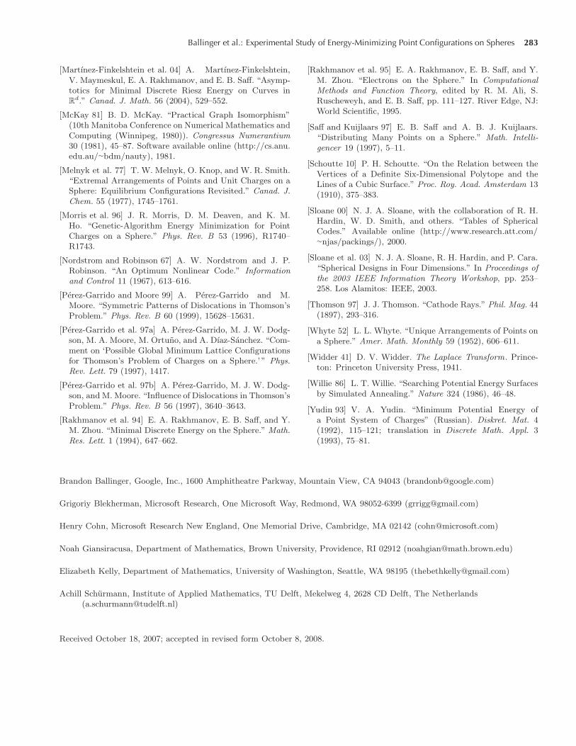
Ballinger et al.: Experimental Study of Energy-Minimizing Point Configurations on Spheres 283
[Martınez-Finkelshtein et al. 04] A. Martınez-Finkelshtein,V. Maymeskul, E. A. Rakhmanov, and E. B. Saff. “Asymp-totics for Minimal Discrete Riesz Energy on Curves inR
d.” Canad. J. Math. 56 (2004), 529–552.
[McKay 81] B. D. McKay. “Practical Graph Isomorphism”(10th Manitoba Conference on Numerical Mathematics andComputing (Winnipeg, 1980)). Congressus Numerantium30 (1981), 45–87. Software available online (http://cs.anu.edu.au/∼bdm/nauty), 1981.
[Melnyk et al. 77] T. W. Melnyk, O. Knop, and W. R. Smith.“Extremal Arrangements of Points and Unit Charges on aSphere: Equilibrium Configurations Revisited.” Canad. J.Chem. 55 (1977), 1745–1761.
[Morris et al. 96] J. R. Morris, D. M. Deaven, and K. M.Ho. “Genetic-Algorithm Energy Minimization for PointCharges on a Sphere.” Phys. Rev. B 53 (1996), R1740–R1743.
[Nordstrom and Robinson 67] A. W. Nordstrom and J. P.Robinson. “An Optimum Nonlinear Code.” Informationand Control 11 (1967), 613–616.
[Perez-Garrido and Moore 99] A. Perez-Garrido and M.Moore. “Symmetric Patterns of Dislocations in Thomson’sProblem.” Phys. Rev. B 60 (1999), 15628–15631.
[Perez-Garrido et al. 97a] A. Perez-Garrido, M. J. W. Dodg-son, M. A. Moore, M. Ortuno, and A. Dıaz-Sanchez. “Com-ment on ‘Possible Global Minimum Lattice Configurationsfor Thomson’s Problem of Charges on a Sphere.’ ” Phys.Rev. Lett. 79 (1997), 1417.
[Perez-Garrido et al. 97b] A. Perez-Garrido, M. J. W. Dodg-son, and M. Moore. “Influence of Dislocations in Thomson’sProblem.” Phys. Rev. B 56 (1997), 3640–3643.
[Rakhmanov et al. 94] E. A. Rakhmanov, E. B. Saff, and Y.M. Zhou. “Minimal Discrete Energy on the Sphere.” Math.Res. Lett. 1 (1994), 647–662.
[Rakhmanov et al. 95] E. A. Rakhmanov, E. B. Saff, and Y.M. Zhou. “Electrons on the Sphere.” In ComputationalMethods and Function Theory, edited by R. M. Ali, S.Ruscheweyh, and E. B. Saff, pp. 111–127. River Edge, NJ:World Scientific, 1995.
[Saff and Kuijlaars 97] E. B. Saff and A. B. J. Kuijlaars.“Distributing Many Points on a Sphere.” Math. Intelli-gencer 19 (1997), 5–11.
[Schoutte 10] P. H. Schoutte. “On the Relation between theVertices of a Definite Six-Dimensional Polytope and theLines of a Cubic Surface.” Proc. Roy. Acad. Amsterdam 13(1910), 375–383.
[Sloane 00] N. J. A. Sloane, with the collaboration of R. H.Hardin, W. D. Smith, and others. “Tables of SphericalCodes.” Available online (http://www.research.att.com/∼njas/packings/), 2000.
[Sloane et al. 03] N. J. A. Sloane, R. H. Hardin, and P. Cara.“Spherical Designs in Four Dimensions.” In Proceedings ofthe 2003 IEEE Information Theory Workshop, pp. 253–258. Los Alamitos: IEEE, 2003.
[Thomson 97] J. J. Thomson. “Cathode Rays.” Phil. Mag. 44(1897), 293–316.
[Whyte 52] L. L. Whyte. “Unique Arrangements of Points ona Sphere.” Amer. Math. Monthly 59 (1952), 606–611.
[Widder 41] D. V. Widder. The Laplace Transform. Prince-ton: Princeton University Press, 1941.
[Willie 86] L. T. Willie. “Searching Potential Energy Surfacesby Simulated Annealing.” Nature 324 (1986), 46–48.
[Yudin 93] V. A. Yudin. “Minimum Potential Energy ofa Point System of Charges” (Russian). Diskret. Mat. 4(1992), 115–121; translation in Discrete Math. Appl. 3(1993), 75–81.
Brandon Ballinger, Google, Inc., 1600 Amphitheatre Parkway, Mountain View, CA 94043 ([email protected])
Grigoriy Blekherman, Microsoft Research, One Microsoft Way, Redmond, WA 98052-6399 ([email protected])
Henry Cohn, Microsoft Research New England, One Memorial Drive, Cambridge, MA 02142 ([email protected])
Noah Giansiracusa, Department of Mathematics, Brown University, Providence, RI 02912 ([email protected])
Elizabeth Kelly, Department of Mathematics, University of Washington, Seattle, WA 98195 ([email protected])
Achill Schurmann, Institute of Applied Mathematics, TU Delft, Mekelweg 4, 2628 CD Delft, The Netherlands([email protected])
Received October 18, 2007; accepted in revised form October 8, 2008.