six-point configurations in the hyperbolic plane and ... - imj-prg
TRANSCRIPT
SIX-POINT CONFIGURATIONS IN THE HYPERBOLIC PLANE AND
ERGODICITY OF THE MAPPING CLASS GROUP
JULIEN MARCHE AND MAXIME WOLFF
Abstract. Let X be the space of isometry classes of ordered sextuples of points in the hyper-bolic plane such that the product of the six corresponding rotations of angle π is the identity.This space X is closely related to the PSL2(R)-character variety of the genus 2 surface Σ. Inthis article we study the topology and the natural symplectic structure on X, and we describethe action of the mapping class group of Σ on X. This completes the classification of the ergodiccomponents of the character variety in genus 2 initiated in [13]. MSC Classification: 58D29,
57M05, 20H10, 30F60.
1. Introduction and statements
1.1. A simple dynamical system. The hyperbolic plane H2 is naturally identified to thesubspace of PSL2(R) consisting of matrices (up to sign) of trace 0, via the map which associatesto a point x ∈ H2 the rotation sx of angle π.
In this article we will be studying the following space of configurations of sextuples,
Sex ={
(x1, . . . , x6) ∈(H2)6 | sx6 · · · sx1 = 1
},
and its quotient X = Sex /PSL2(R) by the natural diagonal action.Given a configuration (x1, . . . , x6) ∈ Sex, and i ∈ {1, . . . , 6}, we may perform a leapfrog move
Li, which consists in replacing xi with xi+1 (in cyclic notation) and xi+1 with sxi+1(xi). In thismove, xi “comes to xi+1 and pushes it by the same motion”: this evokes the leapfrog gameplayed by children, although it may be more accurate to think of a move in Chinese checkers.This move leaves invariant the four other points, as well as the product sxi+1sxi , hence preservesSex. We will denote by Mod(So) the group generated by these leapfrog moves; this notation willbecome clear later.
As a simple example of configuration (x1, . . . , x6) ∈ Sex we may choose x1, x3 and x5 arbi-trarily and set x2 = x1, x4 = x3 and x6 = x5. Such a configuration, as well as all the elementsof their Mod(So)-orbits, will be called pinched configurations. If moreover x1 = x3 = x5 wecall it a singular configuration: these configurations yield the only singular point of X. We willdenote by X∗ the space of isometry classes of non-singular configurations, and by X× the spaceof isometry classes of configurations of six points which do not lie in the same geodesic linein H2.
It will be a simple observation that X has three connected components; we will denote byX0 the one containing the isometry class of singular configurations. We will prove the followingstatements:
Theorem 1.1. Let x ∈ X0 be an isometry class of non-pinched configurations. There is asequence (γn)n≥0 in Mod(So) such that the sequence ([γn ·x])n≥0 converges to the isometry classof the singular configurations. The sequence is provided by a geometric algorithm.
Theorem 1.2. The group Mod(So) acts on X0 ergodically.1
2 JULIEN MARCHE AND MAXIME WOLFF
Along the way, we will show that X0 is homeomorphic to a conical neighbourhood of itssingularity and derive its homeomorphic type.
The space X0, being a real algebraic variety, has a natural (Lebesgue) class of measures forwhich it makes sense, as in Theorem 1.2, to say that the action of Mod(So) is ergodic. Moreover,X∗0 also has a natural symplectic structure, related to its interpretation as a character variety.
1.2. Sextuples and representation spaces. Let Σ be a genus two surface, let Γ denote thefundamental group of Σ, and let X(Γ) = Hom(Γ,PSL2(R))/PSL2(R) be the space of morphismsof Γ in PSL2(R) up to conjugacy. A representation ρ : Γ→ PSL2(R) is called elementary if it has
a finite orbit in H2. Equivalently, ρ is non-elementary if its image is Zariski-dense in PSL2(R).We denote by X×(Γ) the space of conjugacy classes of non-elementary representations. By workof W. Goldman [7] this is a smooth 6-dimensional symplectic manifold.
Let Mod(Σ) be the mapping class group of Σ. By the Dehn-Nielsen-Baer theorem, thisgroup may be viewed as the quotient Out+(Γ) = Aut+(Γ)/ Inn(Γ) of orientation-preservingautomorphisms of Γ up to inner automorphisms. A class [ϕ] ∈ Out+(Γ) acts on a conjugacyclass [ρ] ∈ X(Γ) by the formula [ϕ] · [ρ] = [ρ◦ϕ−1]. In genus two, Mod(Σ) has a special element,the hyperelliptic involution, which generates its center.
The Euler class eu: X(Γ) → {−2,−1, 0, 1, 2} measures the obstruction of lifting the repre-
sentations Γ→ PSL2(R) to the universal cover PSL2(R). By work of W. Goldman [8], for eachk ∈ {−2,−1, 1, 2}, the set X×k (Γ) of classes of representations of Euler class k is connected, and
we proved in [13] that the set X×0 (Γ) splits into two disjoint open sets X+0 (Γ) and X−0 (Γ), that
we denoted byM+ andM−. The hyperelliptic involution fixes X+0 (Γ) pointwise, whereas it acts
on X−0 (Γ) as the conjugation by orientation-reversing isometries of the plane. A consequence of[13], Proposition 1.2, is that both X+
0 (Γ) and X−0 (Γ) are connected. We will discuss briefly thisconnectedness in Section 3.3.
If ϕ ∈ Diff+(Σ) represents the hyperelliptic involution, the quotient So of Σ by the action ofϕ has the structure of a spherical orbifold with six points of order 2. Let Γo denote its orbifoldfundamental group. As Γo has the natural following presentation
Γo = 〈c1, c2, c3, c4, c5, c6 | c2i = 1, c1 · · · c6 = 1〉,
there is an obvious identification between Sex and the space Hom′(Γo,PSL2(R)) of morphismswhich do not kill any of the ci’s, hence the space X is in bijection with the character varietyX(Γo) = Hom′(Γo,PSL2(R))/PSL2(R).
Now if π : Σ → So is the quotient by the action of ϕ, the natural map π∗ : Γ → Γo induces amap π∗ : X(Γo) → X(Γ), which restricts to a canonical identification between X×0 and X+
0 (Γ).Furthermore, this identification is equivariant for the action of the group Mod(Γo) of leapfrogmoves on X×0 , and the action of Mod(Γ) on X+
0 (Γ).
1.3. Dynamics of the mapping class group on PSL2(R)-characters in genus two. In [13]we studied the dynamics of Mod(Σ) on X×(Γ), leaving behind the component X+
0 (Γ). Namely,we proved that Mod(Σ) acts ergodically on each of the components X×−1(Γ), X×1 (Γ) and X−0 (Γ),and proved the related result that every representation in these connected components sendssome simple closed curve to a non-hyperbolic element of PSL2(R). The proof of the ergodicityin [13] is strongly related to the existence of non-separating simple closed curves mapped tonon-hyperbolic elements, which we proved for almost every representation in these components.By Proposition 1.2 of [13], the same technique cannot be applied to representations in X+
0 (Γ).An easy consequence of Theorem 1.1 is that every representation in X+
0 (Γ) sends some sepa-rating simple closed curve either to the identity or to an elliptic element of PSL2(R). Then the
HOURGLASS REPRESENTATIONS 3
techniques for proving the ergodicity of Mod(Σ) are more involved than in [13]. Together withthe results of [13], Theorems 1.1 and 1.2 yield the following statements:
Theorem 1.3. Let ρ : Γ → PSL2(R) be a representation mapping every simple closed curve toa hyperbolic element. Then ρ is faithful and discrete.
Theorem 1.4. The mapping class group Mod(Σ) acts ergodically on each connected componentof non-extremal Euler class of X×(Γ).
Theorem 1.3 gives an affirmative answer to a question of B. Bowditch (see [1], question C)in the genus two case, while Theorem 1.4 proves a conjecture of W. Goldman in the genus twocase.
If a representation ρ : Γ → PSL2(R) sends a separating simple curve to an elliptic element,we may think of the restriction of ρ on the fundamental group of each of the two one-holed torias the holonomy of a conic hyperbolic structure on a torus with one cone point. Thus we maythink geometrically of a generic representation in X+
0 (Γ) as two such tori glued along their conepoints. For this reason, we like to call hourglass these representations.
1.4. Brief outline of the proofs. The dynamical system of sextuples of points in H2 actedon by leapfrog moves is simple enough to find, for every possible non-pinched configuration, anexplicit sequence of leapfrog moves which decreases the sum
∑6i=1 d(xi, xi+1). This is done case
by case, and leads to the proof of Theorem 1.1. This also yields a geometric algorithm which,given any non-elementary representation of Γo in PSL2(R), decides whether it is discrete; thusextending the results of [6] and [5] to the group Γo.
Theorem 1.1 enables to reduce the proof of Theorem 1.2 to a neighbourhood of the singularrepresentation as in [3]. This neighbourhood has several natural, simple and useful interpre-tations. First, as a set of limits of sextuple configurations in H2, it may be thought of as aset of configurations of six points in the Euclidean plane, satisfying extra conditions. Second,following [16] or [7], it can be interpreted in terms of the first cohomology group of Γo in sl2(R)with coefficients twisted by the adjoint action of the singular representation. This leads to athird interpretation as an open set in the cotangent bundle of the Grassmannian of Lagrangiansin the symplectic vector space H1(Σ,R). Each of these three models bears a natural symplec-tic structure, and we prove that the natural symplectic structure on X+
0 (Γ) converges to therelevant natural symplectic form on each model, at the singular representation.
The idea is then to use the Dehn twists along the separating curves which are mapped toelliptic elements. The strategy of the proof, as in [9], is to prove that if [ρ] is sufficientlyclose to the singular class of representations, the corresponding twist flows are transitive on aneighbourhood of [ρ]. In the situation at hand, we do not show whether these twist flows generatethe space of all directions around our representations (contrarily to [9] or [13]), but by using thethird model we prove that their directions generate a completely non-integrable distribution ofdirections, hence these flows are indeed transitive; this leads to the proof of Theorem 1.2.
1.5. Organisation of the article. We introduce some notation in Section 2 and relate oursimple dynamical system to the dynamics of the mapping class group in genus 2. In Section 3,we prove Theorem 1.3. Section 4 is devoted to the neighborhood of the singular configurationwhereas Section 5 contains the proof of Theorem 1.4.
1.6. Acknowledgements. This work was partially supported by the french ANR ModGroupANR- 11-BS01-0020 and SGT ANR-11-BS01-0018. The second author acknowledges support
4 JULIEN MARCHE AND MAXIME WOLFF
from U.S. National Science Foundation grants DMS 1107452, 1107263, 1107367 “RNMS: Geo-metric Structures and Representation Varieties” (the GEAR Network). We would like to thankTian Yang and Dick Canary for their kind interest.
2. Configurations of sextuples
The aim of this section is to expand on the relation, mentionned in the introduction, betweenthe space of sextuple configurations and the PSL2(R)-character variety of the surface of genustwo. We will first elaborate on the presentation of the marked groups Γ and Γo, in order to seethe group of leapfrog moves as a mapping class group. It is actually isomorphic to the 6-strandsbraid group of the sphere. We will then recall some elementary drawings relating products ofhalf-turns; these reminders will be useful later on. We will then expand on the natural mapbetween X(Γo) and X(Γ), and finally exhibit a complete list of types of sextuple configurations,which will be used in the following section.
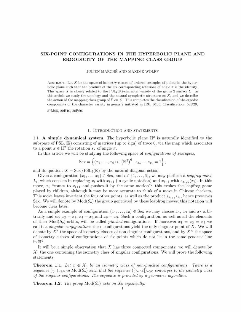
2.1. Markings of the groups Γ and Γo. With suitable markings, the groups Γ and Γo admitthe following presentations,
Γo = 〈c1, c2, c3, c4, c5, c6 | c2i = 1, c1 · · · c6 = 1〉,
Γ = 〈a1, b1, a2, b2 | [a1, b1][a2, b2] = 1〉,and the morphism π∗ associated to the quotient by the hyperelliptic involution is defined asfollows:
(1) π∗(a1) = c1c2, π∗(b1) = c3c2, π∗(a2) = c4c5, π∗(b2) = c6c5.
Figure 1 is meant to help the reader with the above conventions for presenting the groups Γ andΓo. It should be noted here that, since the product in a fundamental group uses concatenationof paths, words in these groups are to be read from left to right, and our convention for thecommutator here is: [a, b] = aba−1b−1. On the other hand, we prefer to think of PSL2(R) as
ϕ∗
b1
a2a1
b2
∗c1
· · · c4· · ·π
ΣSo
Figure 1. Markings of the groups Γ and Γo
acting on H2 on the left, hence we prefer to read words in PSL2(R) from right to left. Forthis reason, we will take the convention that morphisms ρ : Γ → PSL2(R) should be definedas satisfying the relation ρ(αβ) = ρ(β)ρ(α) for all α, β ∈ Γ. We will also denote, for A,B ∈PSL2(R), [A,B] = B−1A−1BA. This convention is reminiscent of [13] or [4].
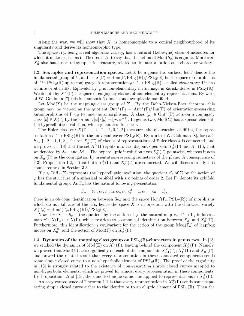
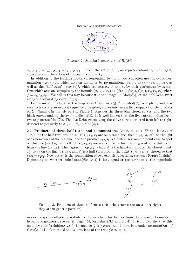
Every positive self-diffeomorphism ψ of Σ commutes, up to isotopy, with the hyperellipticinvolution ϕ, hence descends to a diffeomorphism of the sphere with six marked points. Thisdefines an isomorphism between the quotient Mod(Σ)/[ϕ] and the group B6(S2), the 6-strandsbraid group of the sphere. This group is generated by the “standard” generators, often denotedby σi, as schematised in Figure 2. As they are depicted in Figure 2 the diffeomorphisms σifix the base point of So hence act as automorphisms of Γo; we can read: σi∗(ci) = ci+1 and
HOURGLASS REPRESENTATIONS 5
?
pj
cjpi
pi+1
σi
Figure 2. Standard generators of B6(S2)
σi∗(ci+1) = c−1i+1cici+1 = ci+1cici+1. Hence, the action of σi on representations Γo → PSL2(R)
coincides with the action of the leapfrog move Li.In addition to the leapfrog moves corresponding to the σi, we will often use the cyclic per-
mutation σ5σ4 · · ·σ1, which acts on sextuples by permutation, (x1, . . . , x6) 7→ (x2, . . . , x1), aswell as the “half-twist” (σ1σ2σ1)2, which replaces c1, c2 and c3 by their conjugates by c1c2c3,thus which acts on sextuples by the formula (x1, . . . , x6) 7→ (f(x1), f(x2), f(x3), x4, x5, x6) wheref = sx3sx2sx1 . We call it this way because it is the image, in Mod(So), of the half-Dehn twistalong the separating curve [a1, b1].
Let us insist, finally, that the map Mod(Σ)/[ϕ] → B6(S2) = Mod(So) is explicit, and it iseasy to translate an explicit sequence of leapfrog moves into an explicit sequence of Dehn twistson Σ. Namely, in the left part of Figure 1, consider the three blue closed curves, and the twoblack curves making the two handles of Σ. It is well-known that the five corresponding Dehntwists generate Mod(Σ). The five Dehn twists along these five curves, ordered from left to right,descend respectively to σ1, . . . , σ5 in Mod(So).
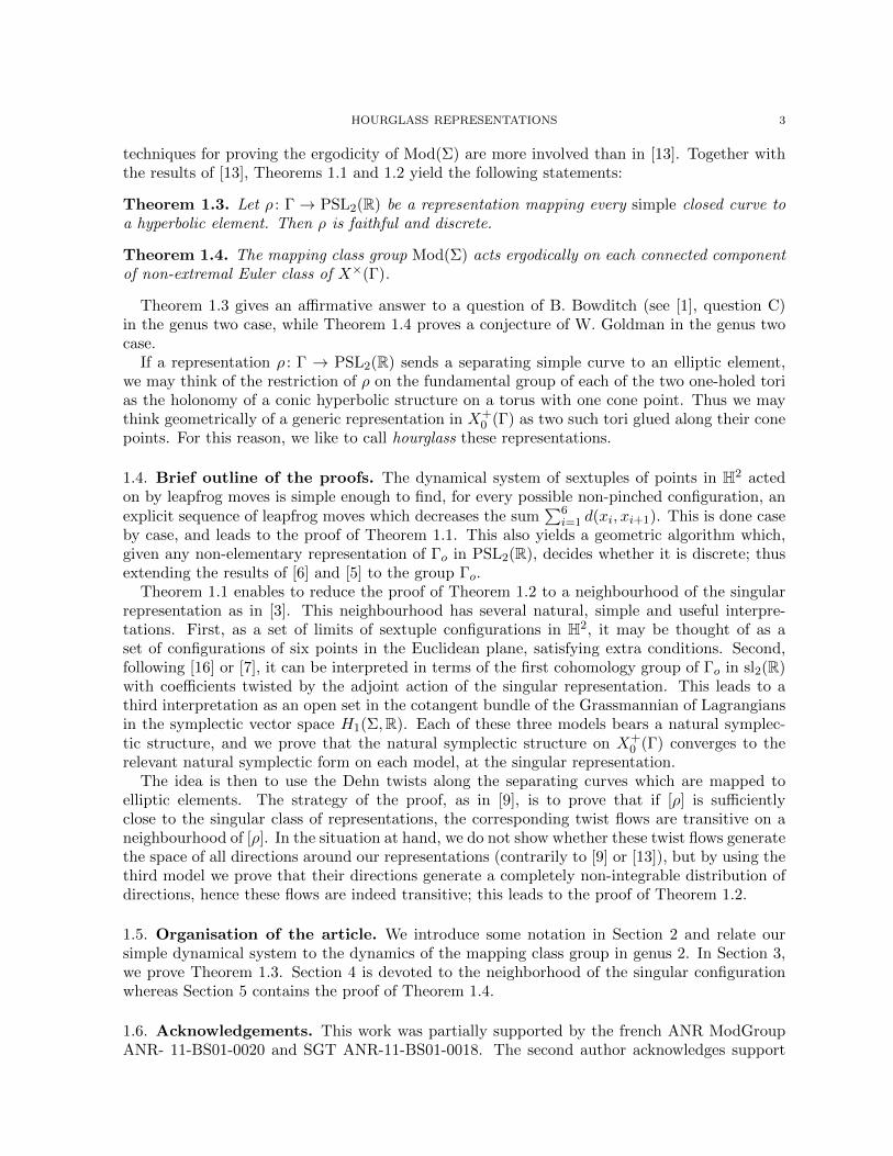
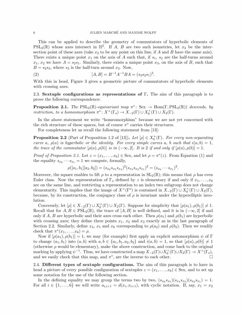
2.2. Products of three half-turns and commutators. Let x1, x2, x3 ∈ H2 and let si, i =1, 2, 3, be the half-turn around xi. If x1, x2, x3 are on a same line, then s1, s2, s3 can be thoughtof as isometries of the real line, and the product s3s2s1 is a half-turn around a point easy to spoton this line (see Figure 3, left). If x1, x2, x3 are not on a same line, then x3 is at some distance hfrom the line (x1, x2). Then s3s2s1 = s3s
′2s′1, where s′2 is the half-turn around the closest point,
x′2, to x3 on the line (x1, x2), and s′1 is a half-turn around the point x′1 ∈ (x1, x2) chosen so thats2s1 = s′2s
′1. Now s3s2s1 is the composition of two explicit reflections, r2r1 (see Figure 3, right).
Depending on whether sinh(h) sinh(d(x1, x2)) is less, equal or greater than 1, the hyperbolic
x1x2
x3
s3s2s1x′2
x′1
x1x2
x3
r2r1
h
Figure 3. Products of three half-turns (left: the centres are on a line; right:they are in generic position)
motion s3s2s1 is elliptic, parabolic or hyperbolic (this follows from the classical formulas inhyperbolic geometry, see eg [2], page 454, formulas 2.3.1 and 2.3.4). It is noteworthy that thisquantity sinh(h) sinh(d(x1, x2)) is equal to 1
2 Tr(s3s2s1) and is invariant under permutations ofthe x′is. It is often called the ∆-invariant of the triangle x1, x2, x3.
6 JULIEN MARCHE AND MAXIME WOLFF
This can be applied to describe the geometry of commutators of hyperbolic elements ofPSL2(R) whose axes intersect in H2. If A, B are two such isometries, let x2 be the inter-section point of these axes (take x2 to be any point on this line, if A and B have the same axis).There exists a unique point x1 on the axis of A such that, if s1, s2 are the half-turns aroundx1, x2 we have A = s2s1. Similarly, there exists a unique point x3, on the axis of B, such thatB = s2s3, where s3 is the half-turn around x3. Now,
(2) [A,B] = B−1A−1BA = (s3s2s1)2.
With this in head, Figure 3 gives a geometric picture of commutators of hyperbolic elementswith crossing axes.
2.3. Sextuple configurations as representations of Γ. The aim of this paragraph is toprove the following correspondence:
Proposition 2.1. The PSL2(R)-equivariant map π∗ : Sex → Hom(Γ,PSL2(R)) descends, byrestriction, to a homeomorphism π∗ : X×(Γo)→ X−2(Γ) ∪X+
0 (Γ) ∪X2(Γ).
In the above statement we write “homeomorphism” because we are not yet concerned withthe rich structure of these spaces, but of course π∗ carries their structures.
For completeness let us recall the following statement from [13]:
Proposition 2.2 (Part of Proposition 1.2 of [13]). Let [ρ] ∈ X+0 (Γ). For every non-separating
curve a, ρ(a) is hyperbolic or the identity. For every simple curves a, b such that i(a, b) = 1,the trace of the commutator [ρ(a), ρ(b)] is in (−∞, 2]. It is 2 if and only if [ρ(a), ρ(b)] = 1.
Proof of Proposition 2.1. Let z = (x1, . . . , x6) ∈ Sex, and let ρ = π∗(z). From Equation (1) andthe equality sx6 · · · sx1 = 1 we compute, formally,
ρ([a1, b1][a2, b2]) = (sx6sx5sx4)2(sx3sx2sx1)2 = (sx6 · · · sx1)2.
Moreover, the square enables to lift ρ to a representation in SL2(R); this means that ρ has evenEuler class. Now the representation of Γo defined by z is elementary if and only if x1, . . . , x6
are on the same line, and restricting a representation to an index two subgroup does not changeelementarity. This implies that the image of X×(Γo) is contained in X−2(Γ) ∪X+
0 (Γ) ∪X2(Γ),because, by its construction, the conjugacy class of ρ is invariant under the hyperelliptic invo-lution.
Conversely, let [ρ] ∈ X−2(Γ) ∪X+0 (Γ) ∪X2(Γ). Suppose for simplicity that [ρ(a1), ρ(b1)] 6= 1.
Recall that for A,B ∈ PSL2(R), the trace of [A,B] is well defined, and it is in (−∞, 2] if andonly if A, B are hyperbolic and their axes cross each other. Then ρ(a1) and ρ(b1) are hyperbolicwith crossing axes; they define three points x1, x2 and x3 exactly as in the last paragraph ofSection 2.2. Similarly, define x4, x5 and x6 corresponding to ρ(a2) and ρ(b2). Then we readilycheck that π∗(x1, . . . , x6) = ρ.
Now if [ρ(a1), ρ(b1)] = 1, we may (for example) first apply an explicit automorphism ψ of Γto change (a1, b1) into (a, b) with a, b ∈ {a1, b1, a2, b2} and i(a, b) = 1, so that [ρ(a), ρ(b)] 6= 1(otherwise ρ would be elementary), make the above construction, and come back to the originalmarking by applying ψ−1. Thus, we have constructed a map X−2(Γ)∪X+
0 (Γ)∪X2(Γ)→ X×(Γo),and we easily check that this map, and π∗, are the inverse to each other. �
2.4. Different types of sextuple configurations. The aim of this paragraph is to have inhead a picture of every possible configuration of sextuples z = (x1, . . . , x6) ∈ Sex, and to set upsome notation for the use of the following section.
In the defining equality we may group the terms two by two, (sx6sx5)(sx4sx3)(sx2sx1) = 1.For all i ∈ {1, . . . , 6} we will write ai,i+1 = d(xi, xi+1), with cyclic notation. If, say, x1 = x2
HOURGLASS REPRESENTATIONS 7
then the above relation implies that x3, x4, x5, x6 are on the same line. In this case, it is easy todeform z among sextuple configurations into a singular configuration. Now we want to describethe generic configurations, in which ai,i+1 6= 0 for all i. We then denote by Di,i+1 the line joiningxi and xi+1. Note that si+1si is a hyperbolic translation along that line.
It is elementary and classical to picture the product of two given hyperbolic motions, saysx2sx1 and sx4sx3 . If their axes D12 and D34 cross each other in H2, we decompose each of thesetwo motions into two rotations of angle π, one of them being around their intersection point (asin Paragraph 2.2). The resulting product is the product of the two other half turns. If D12 andD34 are disjoint in H2 ∪ ∂H2 we decompose each of the two motions into two reflections alonglines, one of them being the common perpendicular H23 of D12 and D34. Then sx6sx5 is theproduct of the reflections along the two other lines, which, therefore, cannot intersect each otherin H2 ∪ ∂H2. It follows that the lines D12, D34 and D56, together with the respective commonperpendiculars H23, H45 and H61, form a right-angled hexagon, which may be regular or skew,depending on whether the directions of the motions sx2sx1 and sx4sx3 agree or disagree (thismakes sense for instance by parallel transport along H23). The only remaining case is when D12
and D34 meet at ∂H2; the motions sx2sx1 and sx4sx3 are then contained in a parabolic subgroupof PSL2(R). The following lemma summarizes the above discussion.
Lemma 2.3. Let z = (x1, . . . , x6) ∈ Sex× be a non-aligned configuration with x1 6= x2, x3 6= x4
and x5 6= x6. Then one of the following holds.
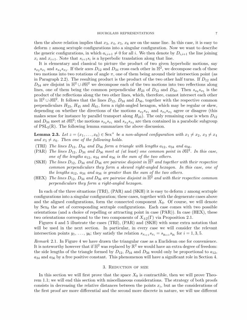
(TRI) The lines D12, D34 and D56 form a triangle with lengths a12, a34 and a56.(PAR) The lines D12, D34 and D56 meet at (at least) one common point in ∂H2. In this case,
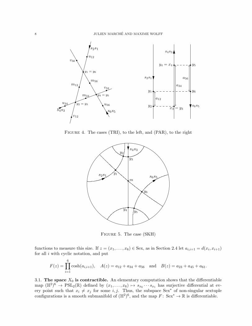
one of the lengths a12, a34 and a56 is the sum of the two others.(SKH) The lines D12, D34 and D56 are pairwise disjoint in H2 and together with their respective
common perpendiculars they form a skewed right-angled hexagon. In this case, one ofthe lengths a12, a34 and a56 is greater than the sum of the two others.
(HEX) The lines D12, D34 and D56 are pairwise disjoint in H2 and with their respective commonperpendiculars they form a right-angled hexagon.
In each of the three situations (TRI), (PAR) and (SKH) it is easy to deform z among sextupleconfigurations into a singular configuration; these cases, together with the degenerate cases aboveand the aligned configurations, form the connected component X0. Of course, we will denoteby Sex0 the set of corresponding sextuple configurations. Each case comes with two possibleorientations (and a choice of repelling or attracting point in case (PAR)). In case (HEX), thesetwo orientations correspond to the two components of X±2(Γ) via Proposition 2.1.
Figures 4 and 5 illustrate the cases (TRI), (PAR) and (SKH) with some extra notation thatwill be used in the next section. In particular, in every case we will consider the relevantintersection points y1, . . . , y6; they satisfy the relation sxi+1sxi = syi+1syi for i = 1, 3, 5.
Remark 2.1. In Figure 4 we have drawn the triangular case as a Euclidean one for convenience.It is noteworthy however that if H2 was replaced by R2 we would have an extra degree of freedom:the side lengths of the triangle formed by D12, D34 and D56 would only be proportional to a12,a34 and a56 by a free positive constant. This phenomenon will have a significant role in Section 4.
3. Reduction of size
In this section we will first prove that the space X0 is contractible, then we will prove Theo-rem 1.1; we will end this section with miscellaneous considerations. The strategy of both proofsconsists in decreasing the relative distances between the points xi, but as the considerations ofthe first proof are more differential and the second more discrete in nature, we will use different
8 JULIEN MARCHE AND MAXIME WOLFF
s2s1
s6s5s4s3
m34
y2 = y3
m12
y1 = y6
m56
y4 = y5
u12
u34 u56
v12
v34
v56
s2s1
s4s3
s6s5
y4 = x4
x3 = y3
y1
y2
y5
y6
a12
a34
a56
Figure 4. The cases (TRI), to the left, and (PAR), to the right
s4s3
s2s1 s6s5m
y1
y2
y3
y4 y5
y6
Figure 5. The case (SKH)
functions to measure this size. If z = (x1, . . . , x6) ∈ Sex, as in Section 2.4 let ai,i+1 = d(xi, xi+1)for all i with cyclic notation, and put
F (z) =6∏i=1
cosh(ai,i+1), A(z) = a12 + a34 + a56 and B(z) = a23 + a45 + a61.
3.1. The space X0 is contractible. An elementary computation shows that the differentiablemap (H2)6 → PSL2(R) defined by (x1, . . . , x6) 7→ sx6 · · · sx1 has surjective differential at ev-ery point such that xi 6= xj for some i, j. Thus, the subspace Sex∗ of non-singular sextupleconfigurations is a smooth submanifold of (H2)6, and the map F : Sex∗ → R is differentiable.
HOURGLASS REPRESENTATIONS 9
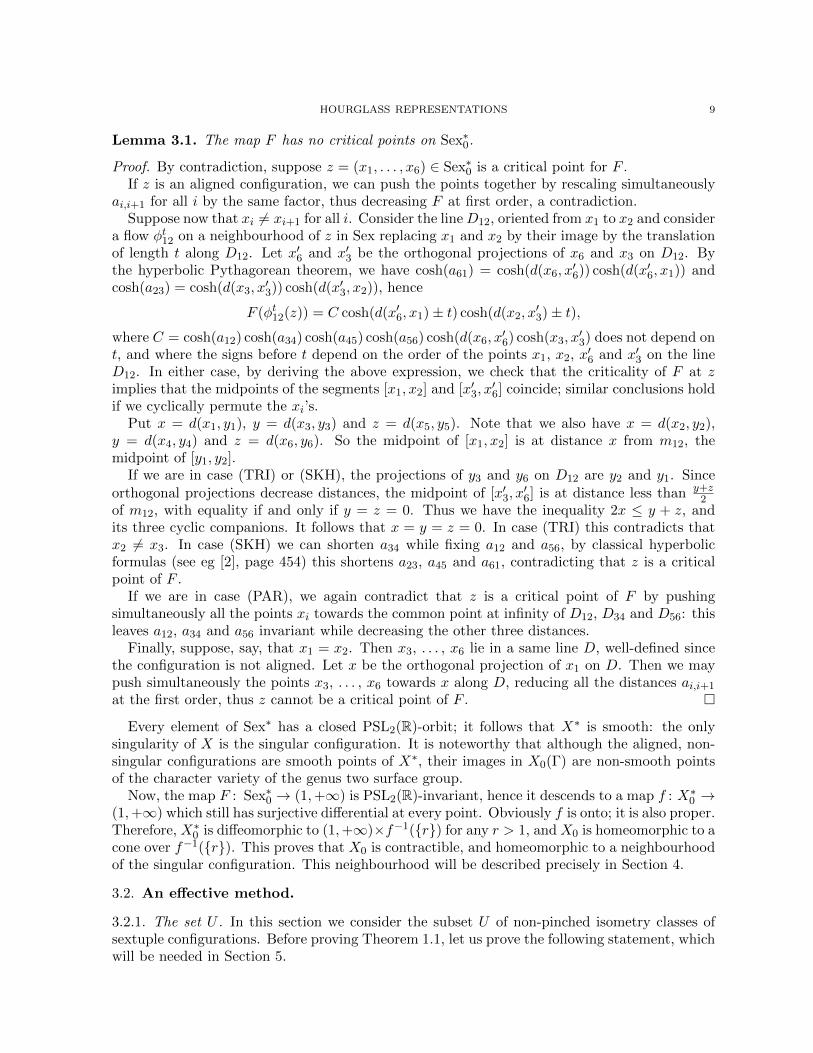
Lemma 3.1. The map F has no critical points on Sex∗0.
Proof. By contradiction, suppose z = (x1, . . . , x6) ∈ Sex∗0 is a critical point for F .If z is an aligned configuration, we can push the points together by rescaling simultaneously
ai,i+1 for all i by the same factor, thus decreasing F at first order, a contradiction.Suppose now that xi 6= xi+1 for all i. Consider the lineD12, oriented from x1 to x2 and consider
a flow φt12 on a neighbourhood of z in Sex replacing x1 and x2 by their image by the translationof length t along D12. Let x′6 and x′3 be the orthogonal projections of x6 and x3 on D12. Bythe hyperbolic Pythagorean theorem, we have cosh(a61) = cosh(d(x6, x
′6)) cosh(d(x′6, x1)) and
cosh(a23) = cosh(d(x3, x′3)) cosh(d(x′3, x2)), hence
F (φt12(z)) = C cosh(d(x′6, x1)± t) cosh(d(x2, x′3)± t),
where C = cosh(a12) cosh(a34) cosh(a45) cosh(a56) cosh(d(x6, x′6) cosh(x3, x
′3) does not depend on
t, and where the signs before t depend on the order of the points x1, x2, x′6 and x′3 on the lineD12. In either case, by deriving the above expression, we check that the criticality of F at zimplies that the midpoints of the segments [x1, x2] and [x′3, x
′6] coincide; similar conclusions hold
if we cyclically permute the xi’s.Put x = d(x1, y1), y = d(x3, y3) and z = d(x5, y5). Note that we also have x = d(x2, y2),
y = d(x4, y4) and z = d(x6, y6). So the midpoint of [x1, x2] is at distance x from m12, themidpoint of [y1, y2].
If we are in case (TRI) or (SKH), the projections of y3 and y6 on D12 are y2 and y1. Sinceorthogonal projections decrease distances, the midpoint of [x′3, x
′6] is at distance less than y+z
2of m12, with equality if and only if y = z = 0. Thus we have the inequality 2x ≤ y + z, andits three cyclic companions. It follows that x = y = z = 0. In case (TRI) this contradicts thatx2 6= x3. In case (SKH) we can shorten a34 while fixing a12 and a56, by classical hyperbolicformulas (see eg [2], page 454) this shortens a23, a45 and a61, contradicting that z is a criticalpoint of F .
If we are in case (PAR), we again contradict that z is a critical point of F by pushingsimultaneously all the points xi towards the common point at infinity of D12, D34 and D56: thisleaves a12, a34 and a56 invariant while decreasing the other three distances.
Finally, suppose, say, that x1 = x2. Then x3, . . . , x6 lie in a same line D, well-defined sincethe configuration is not aligned. Let x be the orthogonal projection of x1 on D. Then we maypush simultaneously the points x3, . . . , x6 towards x along D, reducing all the distances ai,i+1
at the first order, thus z cannot be a critical point of F . �
Every element of Sex∗ has a closed PSL2(R)-orbit; it follows that X∗ is smooth: the onlysingularity of X is the singular configuration. It is noteworthy that although the aligned, non-singular configurations are smooth points of X∗, their images in X0(Γ) are non-smooth pointsof the character variety of the genus two surface group.
Now, the map F : Sex∗0 → (1,+∞) is PSL2(R)-invariant, hence it descends to a map f : X∗0 →(1,+∞) which still has surjective differential at every point. Obviously f is onto; it is also proper.Therefore, X∗0 is diffeomorphic to (1,+∞)×f−1({r}) for any r > 1, and X0 is homeomorphic to acone over f−1({r}). This proves that X0 is contractible, and homeomorphic to a neighbourhoodof the singular configuration. This neighbourhood will be described precisely in Section 4.
3.2. An effective method.
3.2.1. The set U . In this section we consider the subset U of non-pinched isometry classes ofsextuple configurations. Before proving Theorem 1.1, let us prove the following statement, whichwill be needed in Section 5.
10 JULIEN MARCHE AND MAXIME WOLFF
Observation 3.2. The set U is connected, is dense and has full measure in X0.
Proof. Consider the following set P = {(x1, . . . , x6) ∈ Sex |x1 = x2, x3 = x4, x5 = x6, x2 6=x3} of pinched, non-singular configurations. It is a submanifold of dimension 6 of Sex∗, andit descends to a submanifold of dimension 3, hence of codimension 3, of X0. Now U is thecomplement of the orbit of this codimension 3 submanifold, under the countable group Mod(So);the statement of the observation follows. �
Now we turn to the proof of Theorem 1.1, restated as follows.
Theorem 3.3. For all [z] ∈ U , the adherence Mod(So) · [z] contains the isometry class ofsingular configurations.
3.2.2. The operations. To prove this statement we show how to construct an effective “geometricalgorithm” (we will comment later on this terminology) which reduces the size, measured by thefunctions A and B introduced above, of sextuple configurations. Suppose z = (x1, . . . , x6) is anon-aligned sextuple satisfying xi 6= xi+1 for i = 1, 3, 5. Consider the following operations on z,depending on the trichotomy of Lemma 2.3.
(Rot) Make a cyclic permutation, to obtain a sextuple z′ with A(z′) = B(z) and B(z′) = A(z).(Tri) If we are in case (TRI), apply (Rot) an even number of times, so that a12 ≥ a34 and
a12 ≥ a56. Then perform the leapfrog moves L1 to a power minimizing the distanced(x1, y1); apply similarly the moves L3 and L5. Then, if this further decreases B, applyagain L1 or its inverse, once. Then apply (Rot).
(Par) If we are in case (PAR), apply leapfrog moves L3 to push x3 and x4 towards the commonpoint at ∂H2 of D12, D34 and D56, until the distances along horocycles, from x3 or x4,
to D12 and D56, become less than A(z)12 . Then consider the points y1, y2, y5 and y6 as
in Figure 4, and apply powers of L1 and L5 to minimize the distances d(x1, y1) andd(x5, y5). Then apply (Rot).
(Skh0) If we are in case (SKH), first apply (Rot) an even number of times so that a34 > a12+a56,as in Figure 5. Apply powers of L1 and L5 to minimize d(x1, y1) and d(x5, y5). Apply apower of L3 to put x3 in the segment [y3,m] or x4 in the segment [m, y4].
(Skh1) If in case (SKH), apply (Skh0), and then apply the “half-twist move” (L1L2L1)2.
The effect of these operations is precised in the following lemmas.
Lemma 3.4. Suppose z is in case (TRI) or (PAR), and let z′ be the sextuple resulting fromapplying the relevant operation, (Tri) or (Par), to z. Then 24
23A(z′) ≤ B(z′) = A(z).
In the next lemmas, we write bi,i+1 = d(yi, yi+1) for i = 2, 4, 6, in the case (SKH), so that theright-angled skew hexagon has edge lengths ai,i+1 with i = 1, 3, 5 and bi,i+1 with i = 2, 4, 6.
Lemma 3.5. Suppose z is in case (SKH), and let z′ be the sextuple resulting from applyingthe operation (Skh1) to z. Then A(z′) < A(z). More precisely, if a34 > a12 + a56, then theoperation (Skh1) leaves a12 and a56 invariant and decreases cosh(a34) by a quantity larger than
2 sinh2(min(a12,a56))
cosh2(a34). Moreover, provided A(z) is small enough, we also have B(z′) ≤ B(z) +
4A(z)−min(1, b23, b45).
The operations described above do not suffice yet to prove Theorem 1.1; the next lemmaintroduces an additional operation.
Lemma 3.6 (Operation (Skh2)). Provided A(z) and mini=2,4,6(bi,i+1) are small enough, afterapplying (Skh0) the isometry sx′3sx′2sx′1 is a rotation of angle close (but not equal) to π. Then
there exists N ≥ 0 such that (sx′3sx′2sx′1)N is a rotation of angle close to ±π2 and such that the
HOURGLASS REPRESENTATIONS 11
move (L1L2L1)2N results in decreasing A, and such that, if the resulting configuration z′ is stillin case (SKH), then after applying again (Skh0) we have B(z′) ≤ B(z)− 1.
3.2.3. Proof of Theorem 1.1. Let z = (x1, . . . , x6) ∈ Sex such that [z] ∈ U , and let ε > 0, smallenough to apply Lemmas 3.5 and 3.6. We want to prove that there exists z′ ∈ B6(S2) · z suchthat A(z′) +B(z′) ≤ 2ε.
Let us suppose that the configuration is not aligned; we postpone the aligned case to the endof the proof. The case in which xi = xi+1 for some i is quite straightforward and we will dealwith it later. Thus, let us suppose now that our configuration z, as well as all the configurationswe deal with in the following process, satisfy the condition xi 6= xi+1 for all i.
As a first step, let us apply the operations (Tri) or (Par) or (Skh1), depending on whether z isin case (TRI), (PAR) or (SKH) of Lemma 2.3, and iterate this procedure, until A ≤ ε. This firstprocess stops in finite time. Indeed, in cases (TRI) and (PAR), A drops by a factor of at least2423 . The worst thing that could happen is to encounter only the case (SKH) after some iteration.Suppose it is the case. By Lemma 3.5, at each iteration, the three quantities a12, a34 and a56
all decrease, hence the biggest of them stays smaller than the starting quantity A(z). Hence, byLemma 3.5, at each iteration the biggest of cosh(a12), cosh(a34) and cosh(a56) decreases, by anadditive amount depending only on the smallest. Hence, should the process not stop in finitetime, the smallest of a12, a34 and a56 would have to converge to 0. But each iteration changesonly the biggest of a12, a34 and a56. Hence, these three quantities converge to 0, and this firststage of iterations does stop in finite time.
Now we have A(z′) ≤ ε. Of course, under this condition, if we encounter again the case(TRI) or (PAR) then we are done, by Lemma 3.4. Suppose we do not. Proceed as in the firststep until we have min(b23, b45, b61) ≤ ε in case (SKH). This will happen in finite time, by thesecond assertion of Lemma 3.5. Note that the operation (Skh0) leaves A invariant, and afterthis operation we have B ≤ b23 + b45 + b61 + 2A. So as a last step, we proceed by iteratingeither the operation (Skh1), or ((Skh2) followed by (Skh0)), depending on which decreases Bthe most. The conclusions of Lemmas 3.5 and 3.6 now imply that B converges to 0, hence islower than ε after finitely many iterations.
Let us deal now with the case when xi = xi+1 for some i. Up to applying (Rot), suppose thatx5 = x6. Now sx4sx4sx2sx1 = 1, so x1, x2, x3 and x4 have to lie on a same line. Since [z] ∈ U ,these four points need to be pairwise distinct, otherwise we could easily produce leapfrog movesleading to a configuration where xi = xi+1 for i = 1, 3, 5. Denote by ∆ be the line containingx1, . . . , x4 and orient this line. Up to applying powers of L3 we may suppose that x1 is to theleft of x2, x3 and x4 on ∆; this implies that x3 is at the right side of x1, x2, x4. Now putδ1 = d(x1, x2) and δ2 = d(x1, x4). If δ2 > δ1 apply the move L3, this changes (δ1, δ2) into(δ1, δ2− δ1). If δ1 < δ2 apply the move L−1
2 ; this changes (δ1, δ2) into (δ1− δ2, δ2). We recogniseEuclid’s algorithm. It follows from the condition [z] ∈ U that δ1 and δ2 have an irrationalratio, so this process pushes the points x1, x2, x3 and x4 close together. By applying thenpowers of L1 and L3 we may now push these four points as close as we want to the projectionof x5 = x6 on ∆. If x5 = x6 ∈ ∆ then we are done. Otherwise, according to the construction ofSection 2.2, the isometry sx6sx1sx2 is a rotation, of center as close as we want from x5, and ofangle close (but distinct) to π, hence it has an N -th power with angle close to π
2 . Then apply
the iterated half-twist, (L6L1L6)2N . This results in a configuration with A as small as we want(hence A ≤ ε), furthermore in this new configuration the lines (x1, x2) and (x3, x4) now crosseach other, hence this configuration is in case (TRI). Thus, it remains to apply the operation(Tri) in order to get A ≤ ε and B ≤ ε.
12 JULIEN MARCHE AND MAXIME WOLFF
The case of aligned configurations, finally, can be treated by mixing the strategy of case (PAR)and that of the degenerate case above, depending on whether xi = xi+1 for some i. �
3.2.4. Proofs of the lemmas.
Proof of Lemma 3.4. The leapfrog moves L1, L3 and L5 obviously do not change the distancesa12, a34 and a56 summing up to A(z). We need to prove that the moves as in Operations (Tri)and (Par), except the last rotation, lead to a configuration z′ with B(z′) < 23
24A(z). Here we usethe notation z′ even though we may not have reached yet the configuration as in the statementof the lemma; the notation z′ is subject to change in the course of the proof, accordingly to theappropriate moves. We make this abuse of notation here, and in the two subsequent proofs.
Suppose first that z is in the case (TRI). After applying the leapfrog moves minimizingthe distances d(x′i, yi), we have x′i ∈ [ui,i+1,mi,i+1] for i = 1, 3, 5 and x′i ∈ [mi−1,i, vi−1,i] fori = 2, 4, 6, where the points mi,i+1, ui,i+1 and vi,i+1, i = 1, 3, 5 are as in Figure 4. Thus,
d(x′1, y1) ≤ a12
2, d(x′2, y2) ≤ a12
2, d(x′3, y3) ≤ a34
2,
d(x′4, y4) ≤ a34
2, d(x′5, y5) ≤ a56
2, d(x′6, y6) ≤ a56
2.
As y1 = y6, y2 = y3 and y4 = y5 this already gives B(z′) ≤ A(z), by triangular inequalities.If B(z′) ≥ 23
24A(z), then the distances of each x′i to the closest end of its segment sum up to less
than A(z)24 . Suppose (without loss of generality) that a56 ≤ a34 ≤ a12, so that a56 ≤ A(z)
3 . Thesymmetry around y2 and the CAT(0) inequality (and the intercept theorem) imply d(v12, u34) =
d(m12,m34) ≤ a562 . If d(x′2,m12) + d(x′3,m34) ≤ A(z)
24 , or d(x′2, v12) + d(x′3, u34) ≤ A(z)24 , then by
triangle inequalities we get B(z′) ≤ 2124A(z), a contradiction. Thus d(x′2, v12)+d(x′3,m34) ≤ A(z)
24
or d(x′2,m12) + d(x′3, u34) ≤ A(z)24 . After an extra leapfrog move L±1
1 we have again d(x′2, x′3) ≤
a562 + A(z)
24 , and now we only have d(x′1, y1) ≤ a122 + A(z)
24 . Triangle inequalities this time give
B(z′) ≤ 2224A(z); this settles the triangle case.
The parabolic case is much simpler: the inequalities d(y2, x′3) ≤ A(z)
12 , d(x′4, y5) ≤ A(z)12 ,
d(y1, y6) ≤ A(z)6 , d(x′i, yi) ≤ a12
2 for i = 1, 2 and d(x′i, yi) ≤ a562 for i = 5, 6 directly yield,
by triangle inequalities, B(z′) ≤ 56A(z). �
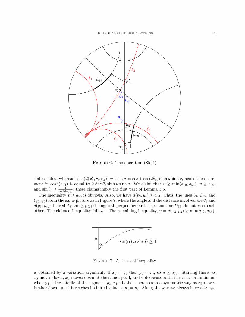
Proof of Lemma 3.5. Let z = (x1, . . . , x5) ∈ Sex be in the (SKH) configuration. Perform themoves according to the operation (Skh1), except the last “half-twist”. Without loss of generality,suppose that now x′3 ∈ [y3,m]. The moves we made so far do not change the value of A, andclearly, the half-twist then does not change the value of a12 or a56. In order to prove the firststatement of Lemma 3.5 we study the effect of this half-twist on a34.
This half-twist amounts to replace x′1, x′2 and x′3 by their image by the isometry sx′3sx′2sx′1 .Recall from Section 2.2 that this isometry is the product r`2r`1 of the reflections by the lines `1and `2, as constructed in Figure 6. Construct, similarly, the lines `3 and `4 such that sx′6sx′5sx′4 =
r`3r`4 . As z ∈ Sex, we have r`1r`2 = r`3r`4 . In particular these four lines either intersect in H2,or in ∂H2, or are all perpendicular to a common line, depending on whether sx′3sx′2sx′1 is elliptic,parabolic or hyperbolic: this is what we observe in Figure 6, but our reasoning will not dependon this trichotomy.
We want to compare a34 with the new distance, d(r`2r`1 ·x′3, x′4). This last distance is equal tod(x′3, r`3r`4 ·x′4) = d(x′3, r`3x
′4). Let p3 ∈ H2 and θ3 ∈ R be as in Figure 6, the intersection point of
`3 and D34 and their angle. Set u = d(x′3, p3) and v = d(p3, x′4). Then cosh(a34) = coshu cosh v+
HOURGLASS REPRESENTATIONS 13
`1
`2
`3
`4
p3
p2
x′3
x′4
a12
a56
θ3
θ2θm
Figure 6. The operation (Skh1)
sinhu sinh v, whereas cosh(d(x′3, r`3x′4)) = coshu cosh v + cos(2θ3) sinhu sinh v, hence the decre-
ment in cosh(a34) is equal to 2 sin2 θ3 sinhu sinh v. We claim that u ≥ min(a12, a56), v ≥ a56,and sin θ3 ≥ 1
cosh(a34) ; these claims imply the first part of Lemma 3.5.
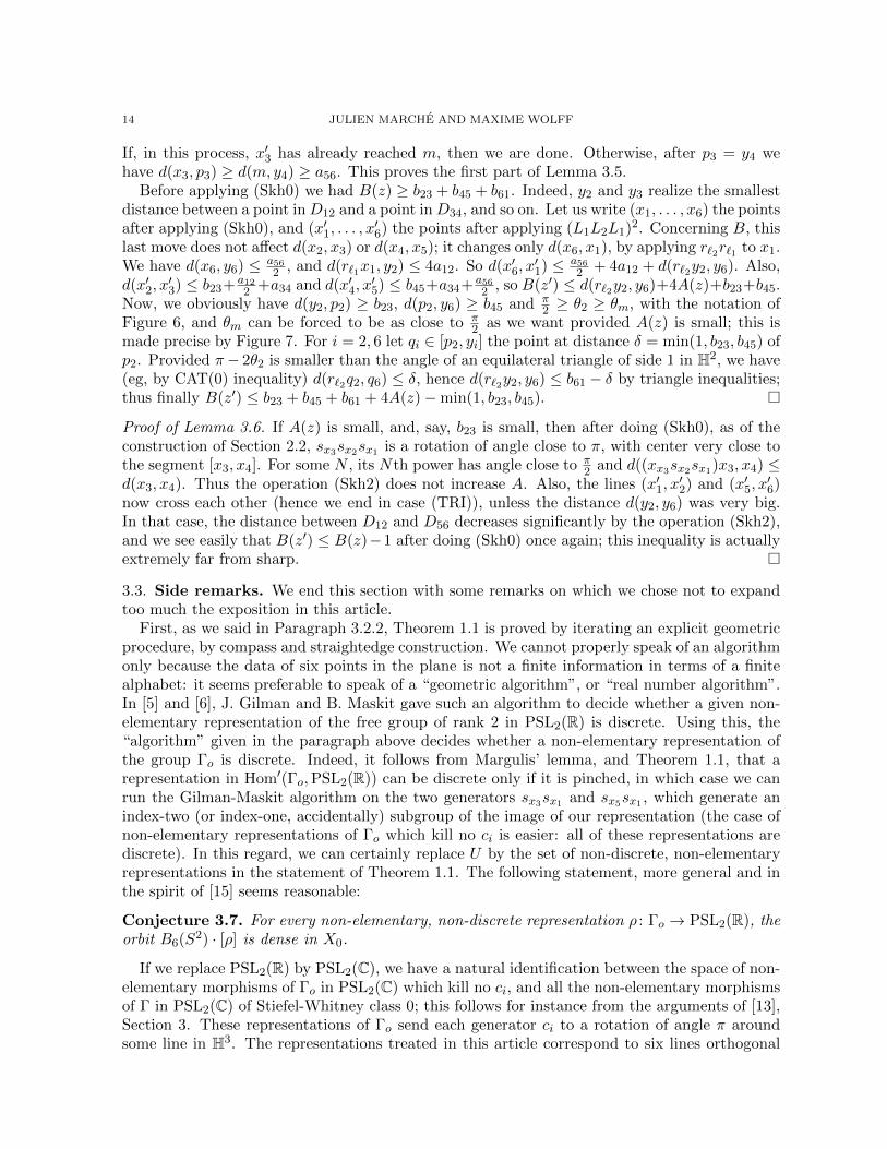
The inequality v ≥ a56 is obvious. Also, we have d(p3, y4) ≤ a34. Thus, the lines `3, D34 and(y4, y5) form the same picture as in Figure 7, where the angle and the distance involved are θ3 andd(p3, y4). Indeed, `3 and (y4, y5) being both perpendicular to the same line D56, do not cross eachother. The claimed inequality follows. The remaining inequality, u = d(x3, p3) ≥ min(a12, a56),
dα
sin(α) cosh(d) ≥ 1
Figure 7. A classical inequality
is obtained by a variation argument. If x3 = y3 then p3 = m, so u ≥ a12. Starting there, asx3 moves down, x4 moves down at the same speed, and v decreases until it reaches a minimumwhen y4 is the middle of the segment [p3, x4]. It then increases in a symmetric way as x3 movesfurther down, until it reaches its initial value as p3 = y4. Along the way we always have u ≥ a12.
14 JULIEN MARCHE AND MAXIME WOLFF
If, in this process, x′3 has already reached m, then we are done. Otherwise, after p3 = y4 wehave d(x3, p3) ≥ d(m, y4) ≥ a56. This proves the first part of Lemma 3.5.
Before applying (Skh0) we had B(z) ≥ b23 + b45 + b61. Indeed, y2 and y3 realize the smallestdistance between a point inD12 and a point inD34, and so on. Let us write (x1, . . . , x6) the pointsafter applying (Skh0), and (x′1, . . . , x
′6) the points after applying (L1L2L1)2. Concerning B, this
last move does not affect d(x2, x3) or d(x4, x5); it changes only d(x6, x1), by applying r`2r`1 to x1.We have d(x6, y6) ≤ a56
2 , and d(r`1x1, y2) ≤ 4a12. So d(x′6, x′1) ≤ a56
2 + 4a12 + d(r`2y2, y6). Also,d(x′2, x
′3) ≤ b23+ a12
2 +a34 and d(x′4, x′5) ≤ b45+a34+ a56
2 , so B(z′) ≤ d(r`2y2, y6)+4A(z)+b23+b45.Now, we obviously have d(y2, p2) ≥ b23, d(p2, y6) ≥ b45 and π
2 ≥ θ2 ≥ θm, with the notation ofFigure 6, and θm can be forced to be as close to π
2 as we want provided A(z) is small; this ismade precise by Figure 7. For i = 2, 6 let qi ∈ [p2, yi] the point at distance δ = min(1, b23, b45) ofp2. Provided π− 2θ2 is smaller than the angle of an equilateral triangle of side 1 in H2, we have(eg, by CAT(0) inequality) d(r`2q2, q6) ≤ δ, hence d(r`2y2, y6) ≤ b61 − δ by triangle inequalities;thus finally B(z′) ≤ b23 + b45 + b61 + 4A(z)−min(1, b23, b45). �
Proof of Lemma 3.6. If A(z) is small, and, say, b23 is small, then after doing (Skh0), as of theconstruction of Section 2.2, sx3sx2sx1 is a rotation of angle close to π, with center very close tothe segment [x3, x4]. For some N , its Nth power has angle close to π
2 and d((xx3sx2sx1)x3, x4) ≤d(x3, x4). Thus the operation (Skh2) does not increase A. Also, the lines (x′1, x
′2) and (x′5, x
′6)
now cross each other (hence we end in case (TRI)), unless the distance d(y2, y6) was very big.In that case, the distance between D12 and D56 decreases significantly by the operation (Skh2),and we see easily that B(z′) ≤ B(z)−1 after doing (Skh0) once again; this inequality is actuallyextremely far from sharp. �
3.3. Side remarks. We end this section with some remarks on which we chose not to expandtoo much the exposition in this article.
First, as we said in Paragraph 3.2.2, Theorem 1.1 is proved by iterating an explicit geometricprocedure, by compass and straightedge construction. We cannot properly speak of an algorithmonly because the data of six points in the plane is not a finite information in terms of a finitealphabet: it seems preferable to speak of a “geometric algorithm”, or “real number algorithm”.In [5] and [6], J. Gilman and B. Maskit gave such an algorithm to decide whether a given non-elementary representation of the free group of rank 2 in PSL2(R) is discrete. Using this, the“algorithm” given in the paragraph above decides whether a non-elementary representation ofthe group Γo is discrete. Indeed, it follows from Margulis’ lemma, and Theorem 1.1, that arepresentation in Hom′(Γo,PSL2(R)) can be discrete only if it is pinched, in which case we canrun the Gilman-Maskit algorithm on the two generators sx3sx1 and sx5sx1 , which generate anindex-two (or index-one, accidentally) subgroup of the image of our representation (the case ofnon-elementary representations of Γo which kill no ci is easier: all of these representations arediscrete). In this regard, we can certainly replace U by the set of non-discrete, non-elementaryrepresentations in the statement of Theorem 1.1. The following statement, more general and inthe spirit of [15] seems reasonable:
Conjecture 3.7. For every non-elementary, non-discrete representation ρ : Γo → PSL2(R), theorbit B6(S2) · [ρ] is dense in X0.
If we replace PSL2(R) by PSL2(C), we have a natural identification between the space of non-elementary morphisms of Γo in PSL2(C) which kill no ci, and all the non-elementary morphismsof Γ in PSL2(C) of Stiefel-Whitney class 0; this follows for instance from the arguments of [13],Section 3. These representations of Γo send each generator ci to a rotation of angle π aroundsome line in H3. The representations treated in this article correspond to six lines orthogonal
HOURGLASS REPRESENTATIONS 15
to a common plane. The representations in X−0 (Γ) correspond to configurations of six lines in aplane; the remaining real characters of representations in SO(3) correspond to six lines througha common point. The quickest proof of the connectedness of X−0 (Γ), to our mind, is throughthis correspondence, by writing, in that setting, the analog of Lemma 2.3; this is all elementaryand we leave the details to the reader. We can extend the methods of Theorem 1.1 to theserepresentations in X−0 (Γ), leading to a much nicer proof of Theorem 1.4 of [13] in the case ofEuler class 0; we chose not to elaborate on this point in this article. It seems more interesting,but also quite challenging, to find a subset of representations in PSL2(C), of positive measure,on which Theorem 1.1 could extend.
4. Neighbourhood of the singular representation
We saw in Theorem 1.1 that the orbit of almost every representation in X0(Γo) accumulates tothe singular representation. The classification of ergodic components of the character varietiestherefore reduces to a careful study of a neighbourhood of the singular representation in X0(Γo).This neighbourhood turns out to have a very rich structure; we devote this section to studyingit. This will provide all the material needed to prove the ergodicity statements in Section 5.
4.1. A Euclidean model. Suppose that zn = (xn1 , . . . , xn6 ) is a sequence of sextuples converging
to the singular configuration. Then, up to extraction and renormalization by a scalar, one cansuppose that the family zn converges in Gromov-Hausdorff sense to a configuration (p1, . . . , p6)in the Euclidean plane E . Consider the set of all limiting configurations up to affine isometryrespecting the orientation: the condition sn6 · · · sn1 = 1 implies the same condition for the Eu-clidean π-rotations over the p′is. This is equivalent to the condition
∑(−1)ipi = 0. Almost
every Euclidean configuration is triangular, and these limits of hyperbolic configurations alsohave to satisfy an extra condition reminiscent from Remark 2.1. We leave it to the reader as apleasant exercise in plane Euclidean geometry that this condition is equivalent to the equalitybetween signed areas as appearing in the following definition:
XE = {(p1, . . . , p6) ∈ E6/∑
(−1)ipi = 0,Area(p1, p2, p3) + Area(p4, p5, p6) = 0}/Isom+(E).
This space is the quotient by a circle action of a quadratic cone inside some vector space V .More precisely, consider the space V = {v = (z1, . . . , z6) ∈ C6/
∑(−1)izi = 0}/C where C acts
on C6 by diagonal translation, and define on V a Hermitian form h as follows:
h(v, v) = Area(z1, z2, z3) + Area(z4, z5, z6)
=1
2det(z2 − z1, z3 − z1) +
1
2det(z5 − z4, z6 − z4)
=1
2
∑1≤i<j≤6
(−1)i+j+1 det(zi, zj) =1
2
∑1≤i<j≤6
(−1)i+j Im(zizj)
=1
4i
∑i<j
(−1)i+j(zizj − zizj).
Also, put q(v) = h(v, v) the underlying real quadratic form and set C = q−1(0). The subset ofnon-aligned sextuples in C will be denoted by C×. With this notation, XE = C/S1 where S1
acts diagonally on V . A simple computation shows that h has signature (2, 2) on V ; in particularit is non-degenerate and its imaginary part gives a symplectic form on the real vector space V ,such that q is a moment map for the diagonal action of S1. This implies that XE has a naturalsymplectic form, being a symplectic quotient; see [14], Section 5.1 for a reminder.
16 JULIEN MARCHE AND MAXIME WOLFF
This symplectic structure has the property that the Hamiltonian flow of the length functiond(z1, z2) (for instance) is the transformation fixing z3, z4, z5, z6 and translating z1 and z2 alongthe line joining them. Moreover, the Hamiltonian flow of the function Area(z1, z2, z3) is givenby
Ψt123(z1, . . . , z6) = (Rtz1, Rtz2, Rtz3, z4, z5, z6)
where Rt is the rotation around the point z1 − z2 + z3 (see Section 2.2).
4.2. The Zariski tangent space. From now on in this section, it will be more convenient
to replace PSL2(R) by its isomorphic group PU(1, 1) =
{±(a b
b a
), a, b ∈ C, |a|2 − |b|2 = 1
}acting by homographies on the unit disc. At a representation ρ, the Zariski tangent space toHom(Γo,PU(1, 1)) may be described as the space of paths ρt : γ 7→ exp(tu(γ))ρ(γ) which, atfirst order, keep being representations of Γo. This condition amounts to the relation u(γ1γ2) =u(γ1) + Adρ(γ1) · u(γ2) for all γ1, γ2 where we have set Adρ(γ) · ξ = ρ(γ)ξρ(γ)−1; the set of suchmaps u is the space Z1(Γo,Adρ) of cocycles in group cohomology with coefficients in pu(1, 1)twisted by the adjoint action of ρ. Coboundaries, of the form γ 7→ u0 − Adρ(γ)u0, correspondto (actual) deformations of ρ by conjugation, and the Zariski tangent space to X(Γo) at a class[ρ] is expected to be isomorphic to H1(Γo,Adρ), see eg [16, 7]. This isomorphism holds at non-elementary representations, by Proposition 5.2 of [10]. In particular, if we denote by the sameletter ρ a representation of Γo and the corresponding representation of Γ, then Proposition 2.1implies that H1(Γo,Adρ) ' H1(Γ,Adρ) at every non-elementary representation.
At singular representations it may happen however that the Zariski tangent is not isomorphicto this cohomology group. We do not investigate this question here, as we are not concernedwith the algebraic structure of X(Γo).
At the singular representation, this cohomology group has a simpler description as we ex-
plain here. Define ρ0 : Γo → PU(1, 1) by ρ(ci) = s0 = ±(i 00 −i
), the half-turn around 0, for
i = 1, . . . , 6. In the natural decomposition pu(1, 1) =
{(ix zz −ix
), x ∈ R, z ∈ C
}' R⊕C, the
element Ad(s0) acts trivialy on R and by multiplication by −1 on C, so the cocycle condition im-plies (with γ1 = γ2 = ci for all i) that every cocycle has a trivial R-part, and (with six terms) that∑
i(−1)iu(ci) = 0, whereas a coboundary sends each ci to the same complex number 2u0; thisgives the natural identification V ' H1(Γo,Adρ0) ' H1(Γo, ε) where by ε we mean C-coefficientstwisted by the action ε(ci)z = −z for i = 1, . . . , 6. This is consistent in idea with the beginning
of Paragraph 4.1. Indeed, the matrix exp
(0 zz 0
)s0 = ±
(i cosh(ρ) −i sinh(ρ)eiθ
i sinh(ρ)e−iθ −i cosh(ρ)
), where
z = ρeiθ, acts on the disc by a half-turn around the point tanh(ρ2)eiθ. Thus, if u is an element of
H1(Γo, ε), the associated deformation ρt maps, at first order, ci to the half-turn around t2u(ci).
Now the inclusion map Γ → Γo yields a map Z1(Γo, ε) → Z1(Γ,C) where the C-coefficientsare not twisted any more since Γ = ker(ε). By checking on a basis, we will prove that this mapinduces an isomorphism as follows.
Proposition 4.1. There is a natural isomorphism between V and the cohomology space H1(Σ,C)such that the Hermitian form h corresponds to the form 1
4iv ·w where · denotes the cup productevaluated at the fundamental class.
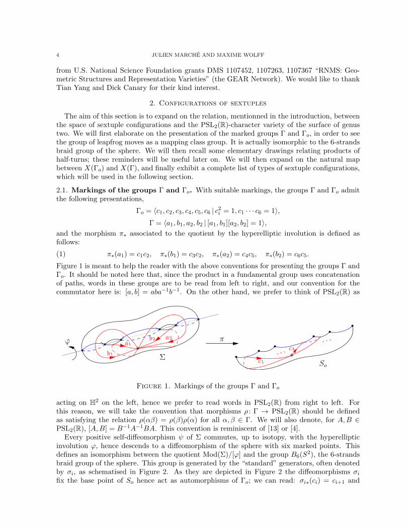
Proof. Let γ1, . . . , γ6 be as in Figure 8 and let γ]i ∈ H1(Σ,C) be the Poincare duals of the
corresponding cycles. From the signed intersections of the γi, we can read γ]i · γ]i+1 = −1,
γ]i · γ]i−1 = 1 for all i (with cyclic notation), and γ]i · γ
]j = 0 if j 6∈ {i − 1, i + 1} mod 6. By
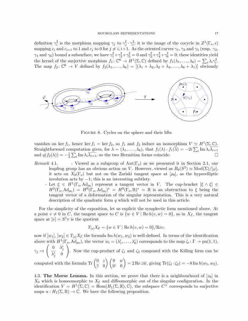
HOURGLASS REPRESENTATIONS 17
definition γ]i is the morphism mapping γj to γ]j · γ]i ; it is the image of the cocycle in Z1(Γo, ε)
mapping ci and ci+1 to 1 and cj to 0 for j 6= i, i+1. As the oriented curves γ1, γ3 and γ5 (resp. γ2,
γ4 and γ6) bound a subsurface, we have γ]1+γ]3+γ]5 = 0 and γ]2+γ]4+γ]6 = 0; these identities yield
the kernel of the surjective morphism f1 : C6 → H1(Σ,C) defined by f1(λ1, . . . , λ6) =∑
i λiγ]i .
The map f2 : C6 → V defined by f2(λ1, . . . , λ6) = [(λ1 + λ2, λ2 + λ3, . . . , λ6 + λ1)] obviously
γ1 γ2γ3 γ4
γ5
γ6ϕ π
pj
pi
pi+1
π(γi)
Figure 8. Cycles on the sphere and their lifts
vanishes on ker f1, hence ker f1 = ker f2, so f1 and f2 induce an isomorphism V ' H1(Σ,C).Straightforward computation gives, for λ = (λ1, . . . , λ6), that f1(λ) · f1(λ) = −2i
∑i Imλiλi+1
and q(f2(λ)) = −12
∑i Imλiλi+1, so the two Hermitian forms coincide. �
Remark 4.1. - Viewed as a subgroup of Aut(Γo) as we presented it in Section 2.1, ourleapfrog group has an obvious action on V . However, viewed as B6(S2) ' Mod(Σ)/[ϕ],it acts on X0(Γo) but not on the Zariski tangent space at [ρ0], as the hyperellipticinvolution acts by −1; this is an interesting subtlety.
- Let ξ ∈ H1(Γo,Adρ0) represent a tangent vector in V . The cup-bracket [ξ ∧ ξ] ∈H2(Γo,Adρ0) = H0(Γo,Adρ0)∗ = H0(Γo,R)∗ = R is an obstruction to ξ being thetangent vector of a deformation of the singular representation. This is a very naturaldescription of the quadratic form q which will not be used in this article.
For the simplicity of the exposition, let us explicit the symplectic form mentioned above. Ata point v 6= 0 in C, the tangent space to C is {w ∈ V | Reh(v, w) = 0}, so in XE , the tangentspace at [v] = S1v is the quotient
T[v]XE = {w ∈ V | Reh(v, w) = 0}/Riv;
now if [w1], [w2] ∈ T[v]XE the formula Imh(w1, w2) is well-defined. In terms of the identification
above with H1(Γo,Adρ0), the vector wi = (λi1, . . . , λi6) corresponds to the map ζi : Γ→ pu(1, 1),
γj 7→(
0 λijλij 0
). Now the cup-product of ζ1 and ζ2 composed with the Killing form can be
computed with the formula Tr
(0 zz 0
)(0 ww 0
)= 2 Re zw, giving Tr(ζ1 · ζ2) = −8 Imh(w1, w2).
4.3. The Morse Lemma. In this section, we prove that there is a neighbourhood of [z0] inX0 which is homeomorphic to XE and diffeomorphic out of the singular configuration. In theidentification V = H1(Σ,C) = Hom(H1(Σ,R),C), the subspace C× corresponds to surjectivemaps u : H1(Σ,R)→ C. We have the following proposition.
18 JULIEN MARCHE AND MAXIME WOLFF
Proposition 4.2. There exist neigbourhoods U of 0 in C, and W of ρ0 in Hom(Γo,PU(1, 1))which are S1-invariant, and an S1-equivariant homeomorphism f : U →W which
(1) is a diffeomorphism on U \ {0} to W \ {ρ0},(2) induces a diffeomorphism between (U \ {0})/S1 and (W \ {ρ0})/S1,(3) maps bijectively C× ∩ U to Hom×(Γo,PU(1, 1)) ∩W .
Proof. In this proof, we denote s0 =
(i 00 −i
)and for any z1, . . . , z6 ∈ C we set ξj =
(0 zjzj 0
).
We will look for a representation ρ ∈ Hom(Γo,PU(1, 1)) such that ρ(cj) = ± exp(ξj)s0. For thatreason, we define in a neighbourhood of 0 a map F : C6 → C and a map ϕ : C6 → R by theformula
exp(ξ6)s0 · · · exp(ξ1)s0 = − exp
(iϕ FF −iϕ
).
We observe that conjugating the equation by the matrix
(eiθ 00 e−iθ
)changes zj to e2iθzj , F to
e2iθF and does not change ϕ. Hence the map ϕ is S1-invariant and the map F is S1-equivariant.We have − exp(ξ6) · · · s0 exp(ξ1)s0 = exp(ξ6) exp(−ξ5) exp(ξ4) exp(−ξ3) exp(ξ2) exp(−ξ1) and
its logarithm is∑
i(−1)iξi +∑
j>i12 [(−1)jξj , (−1)iξi] up to order 2 terms thanks to the Baker-
Campbell-Hausdorff formula. Hence, the Taylor expansion gives F (z1, . . . , z6) =∑6
i=1(−1)izi +o(|z|) and ϕ(z1, . . . , z6) = −2q(z) + o(|z|2).
Consider the map H : C6 → C6 given by H(z1, . . . , z6) = (z1, . . . , z5, F (z1, . . . , z6)). By theinverse function theorem, this is a local diffeomorphism. We observe that by construction, themap F is S1-equivariant, hence the map H and its inverse are also S1-equivariant. For smallenough w′s, write ψ(w2, . . . , w5) = ϕ(H−1(0, w2, w3, w4, w5, 0)). The S1-invariant function ψ :C4 → R has a non-degenerate Hessian at 0 and vanish identically if the w′is are real. We concludeby applying the Morse Lemma 4.3. Indeed, if we denote by Φ the diffeomorphism provided bythe lemma, we simply set f(w2, w3, w4, w5) = H−1(0, x2, x3, x4, x5, 0) where (x2, x3, x4, x5) =Φ(w2, w3, w4, w5).
The sextuples (z1, . . . , z6) ∈ R6 correspond to linear maps v : H1(Σ,R) → C with values inR. Hence, the S1-orbit of real configurations correspond precisely to linear maps of rank 0 or 1and the diffeomorphism f preserve aligned configurations as expected. �
Observe that in the above computation, q appears as a second order obstruction for a co-cycle from being realized by deformations of representations; this is yet another language forunderstanding this quadratic form.
Lemma 4.3 (Equivariant Morse Lemma). Let ϕ : Cn → R be a smooth S1-invariant function,vanishing on Rn and such that ϕ(z) = Q(z) + o(|z|2) for a non-degenerate Hermitian formQ. Then there exist S1-invariant neighbourhoods U and V of 0 in Cn and an S1-equivariantdiffeomorphism Φ : U → V such that
- D0Φ is the identity,- Φ preserves Rn,- ϕ ◦ Φ(z) = Q(z) for z ∈ U .
Proof. This is a variation of the standard Morse Lemma with the same proof, using Moser’strick, see [12], Theorem 3.44. It is sufficient to check that the solution provided by the proofhas the properties required by the lemma. �
We observe that the space X×(Γo) as a subspace of X(Σ) is endowed with the Atiyah-Bottsymplectic structure denoted by ωAB. On the other hand, we explained thatXE is also symplectic
HOURGLASS REPRESENTATIONS 19
with a symplectic structure denoted by ω. We do not know whether one can make the localdiffeomorphism f symplectic but we will at least need the following weaker statement:
Lemma 4.4. The map f constructed in Proposition 4.2 is a symplectomorphism at first orderby which we mean that the following holds:
(f∗ωAB)v = −8ω + o(v).
Proof. Following Goldman (see [7]), the Atiyah-Bott structure at [ρ] ∈ X×(Σ) is induced bythe cup-product on H1(Σ,Adρ) followed by the trace. The claimed approximation follows fromProposition 4.2 and the computation ending Subsection 4.2. �
4.4. The Grassmannian of Lagrangians. There is yet another description of the space X×Eof non-aligned Euclidean configurations which will be crucial in the last step of the proof ofTheorem 1.2. It uses the Grassmannian of Lagrangians in H1(Σ,R) denoted by L. It is a3-dimensional manifold and the tangent space at L ⊂ H1(Σ,R) is canonically isomorphic tothe space of quadratic forms on L. Indeed, the tangent space at L to the Grassmannian of2-planes is canonically isomorphic to the space Hom(L,H1(Σ,R)/L) ' Hom(L,L∗), where weidentify H1(Σ,R)/L with L∗ by the symplectic pairing, and the Lagrangian condition amountsto the symmetry of the corresponding bilinear maps. Dually, the cotangent space of L at L isisomorphic to the space of quadratic forms on the dual space L∗. We denote by T ∗+L ⊂ T ∗L theset of pairs (L,α) where α is a positive definite quadratic form on L∗.
Proposition 4.5. There is a diffeomorphism Λ : X×E → T ∗+L which is equivariant with respectto the action of Sp(H1(Σ,R)).
Proof. Recall that an element of X×E is the S1-orbit of a surjective linear map u : H1(Σ,R)→ Csatisfying q(u) = 0. Set L = keru and show that q(u) = 0 if and only if L is Lagrangian.
The quantity q(u) is computed from any symplectic basis a1, b1, a2, b2 of H1(Σ,R) by the
formula q(u) = 14 Im(u(a1)u(b1) + u(a2)u(b2)). If L is Lagrangian, we can ensure that a1, a2
form a basis of L and hence u(a1) = u(a2) = 0 and q(u) = 0. If L is not Lagrangian, it issymplectic and we can form a basis of L with a1 and b1, which implies that u(a2) and u(b2) arelinearly independent and hence q(u) 6= 0.
Hence, given u : H1(Σ,R) → C with q(u) = 0 and L its (Lagrangian) kernel, the expressionα(x) = |u(x)|2 is a positive definite quadratic form on H1(Σ,R)/L ' L∗, hence α belongs toT ∗+L and does not change if we multiply u by a phase. This construction can be easily reversedand is symplectically invariant hence the map Λ : u 7→ (L,α) has the required properties. �
Lemma 4.6. The map Λ is a symplectomorphism up to a constant.
Proof. Let (L, g) be any point in T ∗+L, one can find a symplectic basis such that L = Span(a1, a2)and a∗1, a
∗2 is an orthonormal basis of L∗ with respect to g. The map u = Λ−1(L, g) is given
by u(a1) = u(a2) = 0, u(b1) = 1, u(b2) = i. There is a local coordinate system (pi, qi)i=1,2,3 onT ∗L given by setting Lp = Re1 ⊕ Re2 where e1 = (1, 0, p1, p2), e2 = (0, 1, p2, p3) and gq has
the matrix
(q1 q2
q2 q3
)in the basis e∗1, e
∗2. In that coordinate system, the symplectic form reads
ωL = Tr dgp ∧ dgq = dp1 ∧ dq1 + 2dp2 ∧ dq2 + dp3 ∧ dq3.The map up,q = Λ−1(Lp, gq) is defined by sending e1 and e2 to 0 and e3, e4 to any basis vq1, v
q2
of R2 whose Gram matrix is gq. Explicitly one has
up,q(a1) = −p1vq1 − p2v
q2, up,q(a2) = −p2v
q1 − p3v
q2, up,q(b1) = vq1, up,q(b2) = vq2.
20 JULIEN MARCHE AND MAXIME WOLFF
Writing as a vector the values taken on the symplectic basis we get at (0, 0, 0, 1, 0, 1) the followingderivatives:
∂Λ−1
∂p1= (−1, 0, 0, 0),
∂Λ−1
∂p2= (−i,−1, 0, 0),
∂Λ−1
∂p3= (0,−i, 0, 0).
Using the formulas∂vq1∂q1
= 12 ,
∂vq1∂q2
=∂vq1∂q3
= 0 and∂vq2∂q1
= 0,∂vq2∂q2
= 1,∂vq2∂q3
= i2 we get
∂Λ−1
∂q1= (0, 0,
1
2, 0),
∂Λ−1
∂q2= (0, 0, 0, 1),
∂Λ−1
∂q3= (0, 0, 0,
i
2).
On the other hand, the symplectic structure on V reads
(3) ωV (v, w) = −〈v(a1), w(b1)〉+ 〈w(a1), v(b1)〉 − 〈v(a2), w(b2)〉+ 〈w(a2), v(b2)〉.By checking in the basis, we find Λ∗ωV = 1
2ωL as asserted. �
4.5. Topology of hourglasses.
Proposition 4.7. The space X0 is homeomorphic to XE . The homeomorphism maps the con-figuration [ρ0] to 0, and C×/S1 to X×0 . In particular we have:
- X∗0 is connected, simply connected and satisfies π2(X∗0 ) = Z.- X×0 is homotopically equivalent to L. Hence it is connected and satisfies π1(X×0 ) =π2(X×0 ) = Z.
Proof. By Proposition 4.2, a punctured neighbourhood of ρ0 is diffeomorphic to X∗E . As we sawin Section 3.1, X∗0 is diffeomorphic to the set f−1(1, 1 + ε) for any ε and the result follows.The Hermitian form h has signature (2, 2) hence in some coordinates one has q(z1, w1, z2, w2) =|z1|2 + |z2|2 − |w1|2 − |w2|2. Normalizing the non-zero vectors (z1, z2) and (w1, w2) we get thehomeomorphism C∗ ' S3×S3×R and hence the homotopy equivalence X∗0 ' S3×S3/S1. Thelong exact sequence of the fibration S3 × S3 → (S3 × S3)/S1 gives the fundamental groups ofX∗0 claimed in the proposition.
Using the canonical Riemannian metric on X∗0 , the gradient flow of f preserves the set ofsextuples which are on the same line. Hence the same argument as above works for the spaceX×0 which is homeomorphic to C×/S1. This latter space is homeomorphic to T ∗+L which is a
fiber bundle over L with convex fiber. Finally we have the homotopy equivalence X×0 ' L.Considering the two-fold covering of L consisting of oriented Lagrangians in H1(Σ,R), we get a
space L = U(2)/SO2, see [14], Section 2.3. The exact sequence of this fibration gives π1(L) 'π2(L) ' Z and the same is true for L. �
5. Dynamics
5.1. The strategy. As in all proofs of ergodicity of mapping group actions on representationspaces, we will use the periodicity properties of Goldman twist flows. These flows are particularlysimple to describe in the framework of sextuples. Let z = (x1, . . . , x6) ∈ Sex0 be a sextuple andsuppose that s3s2s1 is an elliptic element, that is a rotation over a point y. Denote by Rt therotation of angle t over y and pick θ such that s3s2s1 = Rθ. Then the formula
Φt123z = (Rtx1, Rtx2, Rtx3, x4, x5, x6)
defines a 2π-periodic flow on X0 such that Φθ123 is the half-twist around the first three points.
A Mod(So)-invariant function on X0 is almost everywhere constant along the flow as the angleθ is almost everywhere irrational. However this argument works only when s3s2s1 is elliptic.
All such flows are indexed by partition curves, that is simple curves γ in Sp, the sphere minusthe six marked points, which divide the set of points into two subsets of cardinality 3. Indeed,
HOURGLASS REPRESENTATIONS 21
for any [ρ] ∈ X0(Γo) we set Θγ([ρ]) ∈ R/2πZ to be the rotation number of ρ(γ) (that is its angleif it is a rotation and 0 otherwise). Where Θγ is smooth, we define Xγ to be the symplecticgradient of Θγ and extend it by 0 where it is not defined. We denote by Φt
γ the flow of Xγ . Thisdefinition is coherent in the sense that Φ123 = Φγ for a standard partition curve enclosing the 3first points.
Remark 5.1. Let γ be the preimage of γ in the surface Σ: then Φtγ is the Goldman flow on X(Σ)
associated to the separating curve γ provided that ρ(γ) is elliptic.
Definition 5.1. For any z ∈ X0 we set
Dz = Span{Xγ(z), γ partition curve} ⊂ TzX0.
The aim of this section is to prove the following proposition:
Proposition 5.1. The distribution D is completely non-integrable on the subset U ⊂ X0 ofnon-pinched configurations.
By construction, the distribution is Mod(Γo)-invariant, and by Theorem 1.1, the Mod(Γo)-orbit of any point in U is adherent to the singular representation [ρ0]. Hence it is sufficient toprove Proposition 5.1 by replacing U with any neighbourhood of [ρ0]. This will be a significantsimplification for two reasons:
(1) For any partition curve γ, ρ(γ) is elliptic for ρ close enough to ρ0, hence the vector fieldsXγ will not vanish close to the singular representation.
(2) Being completely non-integrable is an open condition, hence, we can replace the functionsΘγ by their Taylor expansion around [ρ0] and reduce the problem to (symplectic) linearalgebra.
The proof of Proposition 5.1 is decomposed into two subsections: in Subsection 5.2 we computethe Taylor expansion of the trace function associated to a partition curve and in Subsection 5.3,we show that the derivatives of these trace functions generate the cotangent space around [ρ0].
To conclude this subsection, we recall the argument showing that Proposition 5.1 impliesthe ergodicity of Mod(Γo) on X0. Let f : X0 → R be a measurable invariant function. Usingstandard ergodicity arguments (see Proposition 5.4 in [9]), for any partition curve γ, there isa measure 0 subset Nγ ⊂ X0 × R such that f(Φt
γ(z)) = f(z) for all (z, t) /∈ Nγ . Using Fubinitheorem and the fact that the flows preserve nullsets, for any partition curves γ1, . . . , γn, we willhave f ◦ Φt1
γ1 ◦ · · ·Φtnγn(z) = f(z) for almost all (z, t1, . . . , tn) ∈ X0 × Rn.
Using cutoff functions one can smoothen the vector fieldsXγ without changing the distributionD - hence we suppose that the vector fields are smooth from now. Let z ∈ X0 be a point in U .By the orbit theorem (see [11], Theorem 1 p.33), the orbit N of z through the action of the flowsof Xγ is a submanifold. By Proposition 5.1, the vector fields Xγ and their brackets evaluatedat z generate TzX0. Hence N is an open subset of X0. Moreover the proof of the orbit theoremin [11] shows that for any z′ ∈ N there exist n ∈ N, curves γ1, . . . , γn and (t01, . . . , t
0n) ∈ Rn such
that the map F : Rn → N defined by
F (t1, . . . , tn) = Φt1γ1 ◦ · · · ◦ Φtn
γn(z)
satisfies F (t01, . . . , t0n) = z′ and rankDF (t01, . . . , t
0n) = dimN = 6. From the fact that f is almost
constant in the image of F , we get that f is almost everywhere constant in a neighborhood ofz′, hence in N , a neighborhood of z.
By Proposition 5.1, this argument works for any point in the connected set U which has fullmeasure, showing that f is almost everywhere constant.
22 JULIEN MARCHE AND MAXIME WOLFF
Remark 5.2. In the spirit of Section 3 we can imagine a proof by hand of the transitivity of theflows Φt
γ . This proof of Theorem 1.2 would be slightly more direct but less informative aboutthe structure of these hourglass representations, and we chose not to develop it here.
5.2. Taylor expansion of trace functions. The set
Sex = {ρ : π1(Sp)→ SL2(R) such that Tr ρ(ci) = 0 for i = 1, . . . , 6}.yields a regular covering of X0, which is contractible as we proved in Section 3.1. Thus, wemay choose once for all a lift ρ0 of the singular representation, and lift every representationρ accordingly. With this setting, for any partition curve γ, we set Fγ([ρ]) = Tr ρ(γ). This isa continuous function on X0, smooth on X×0 and which vanishes at [ρ0]. Our purpose is tocompute its Taylor expansion at [ρ0].
Proposition 5.2. For any partition curve γ ⊂ Sp, let γ ⊂ Σ be its (separating) pre-imagein Σ. Then Σ can be written as Σ′ ∪γ Σ′′. Write ξ ∈ C as ξ = ξ′ + ξ′′ using the decompo-sition H1(Σ,C) = H1(Σ′,C) ⊕ H1(Σ′′,C) and set qγ(ξ) = q(ξ′), then in the chart given byProposition 4.2 we have
Fγ(ξ) = ±8qγ(ξ) + o(|ξ|2).
Proof. Remark that as ξ is in C, we have q(ξ) = q(ξ′) + q(ξ′′) = 0, hence we can replace ξ′ withξ′′ in this formula. Up to the action of Mod(Σ) we can suppose that γ = c1c2c3. The samedirect computation as in the proof of Proposition 4.2 then gives
Tr ρ(c1)ρ(c2)ρ(c3) = ±Tr(eξ1e−ξ2eξ3s0) = ±1
2Tr s0([ξ1, ξ3]− [ξ1, ξ2]− [ξ2, ξ3]) + o(|ξ|2)
= ±∑
1≤j<k≤3
(−1)j+k(zjzk − zkzj) + o(|ξ|2) = ±8q(z1, z2, z3, 0, 0, 0) + o(|ξ|2),
with the same notation. �
The computation here relates the splitting of q into two terms with the orthogonal decompo-sition of the cohomology space. We already saw this splitting in the first definition of XE wherethe quadratic constraint appeared as a sum of two areas.
5.3. Generating the cotangent space. Let us go back to the proof of Proposition 5.1. Werecall that it amounts to proving that the Hamiltonian vector fields Xγ of the functions Fγgenerate a completely non-integrable distribution close enough to the singular configuration.Using Proposition 5.2 and the fact that being completely non-integrable is an open condition,it reduces to proving the following proposition:
Proposition 5.3. For any partition curve γ, let Yγ be the Hamiltonian vector field of thefunction qγ. For any z ∈ X×E , set
Ez = Span{Yγ(z), γ partition curve} ⊂ TzX×E .Then, E is a completely non-integrable distribution on X×E .
Proof. First, we recall that through the symplectic isomorphism TX×E ' T ∗X×E , the vector fieldYγ corresponds to the covector dqγ . Hence, the symplectic orthogonal Eω to the distribution Ehas the following description:
Eωz = {w ∈ TzX×E , Dzqγ(w) = 0,∀γ partition curve in Sp}.We will use the model X×E = C×/S1 where C× is the set of surjective maps v : H1(Σ,R)→ C
such that q(v) = h(v, v) = 0, with h(v, w) = − i4v · w. Recall that a vector w is tangent to C at
v 6= 0 if Reh(v, w) = 0.
HOURGLASS REPRESENTATIONS 23
Lemma 5.4. Let v ∈ C× and let w ∈ V be tangent to C at v and satisfy Dqγ(v)(w) = 0 forany partition curve γ. Then v and w, as linear maps from H1(Σ,R) to R2, satisfy the followingequation:
(4) ∀x, y ∈ H1(Σ,R), det(v(x), w(y)) = det(v(y), w(x)).
Proof. First, observe that for any symplectic basis a1, b1, a2, b2 of H1(Σ,R) we have
−4 Reh(v, w) = det(v(a1), w(b1))− det(v(b1), w(a1)) + det(v(a2), w(b2))− det(v(b2), w(a2)).
Now, for any partition curve γ, let pγ ∈ End(H1(Σ,C)) be the (h-orthogonal) projection onH1(Σ′,C) parallel to H1(Σ′′,C); note that Reh(pγ(·), ·) is a symmetric bilinear form, associatedto qγ . Hence the condition Dqγ(v)(w) is equivalent to Reh(pγ(v), w) = 0. If we choose x = a1
and y = b1 this condition is equivalent to Equation (4).The same holds if we replace (x, y) with its image by any transformation in Sp(4,Z). So the
map Sp(4,R)→ R sending g to det(v(gx), w(gy))− det(v(gy), w(gx)) vanishes on Sp(4,Z). Bythe Zariski-density of Sp(4,Z) in Sp(4,R), this forces Equation (4) to hold for any x, y ∈ H1(Σ,R)such that x · y = 1. By scaling x or y, this holds finally for any x and y and the lemma isproved. �
Fix v : H1(Σ,R) → C surjective and satisfying q(v) = 0. Recall from Subsection 4.4 that itskernel L has to be Lagrangian. Let w be in Eωv : Lemma 5.4 implies that w vanishes on L. Hence,f = w◦v−1 is a well defined endomorphism of R2 and writing x = v−1(x′) and y = v−1(y′) we getdet(f(x′), y′)+det(x′, f(y′)) = 0. Hence, f preserves infinitesimally the form det, or equivalentlyhas vanishing trace. On the other hand, the equation Reh(v, w) = 0 is automatically satisfiedin the preceding conditions. To sum up we have shown that the orthogonal distribution Eωv isthe following 2-dimensional space:
Eωv = {w ∈ Hom(H1(Σ,R),C), w|ker v = 0,Tr(w ◦ v−1) = 0}/Riv.If u ∈ Hom(H1(Σ,R),C) satisfies u|L = 0 then Reh(u, v) = 0. All such maps form a
Lagrangian containing Eωv . It follows that Ev contains this 3-dimensional space. This impliesthat one can express that u belongs to Ev by looking at the restriction of u to L.
Let us show that one has the following description:
(5) Ev = {u ∈ Hom(H1(Σ,R),C) s.t. ∃λ ∈ R, u|L = λ(v∗)−1}.In this formula, we see v as a map H1(Σ,R)/L → C and identify H1(Σ,R)/L with L∗ via theintersection form. Consider an adapted symplectic basis a1, b1, a2, b2 of H1(Σ,R). An elementw in Eωv vanishes on a1, a2 and its matrix M = (w(b1), w(b2)) has trace 0. Let u be in Ev andset N = (u(a1), u(a2)). From the expression of symplectic structure given by equation (3), wederive that the equation TrMN = 0 should be satisfied for all M with 0 trace. Hence N is ascalar matrix and the formula is proved.
This defines a 4-dimensional distribution on C×/S1. It remains to show that it is completelynon-integrable which is the content of the last lemma. �
Lemma 5.5. Let L be the Grassmanian of all Lagrangian subspaces of H1(Σ,R). Recall theidentification X×E : C×/S1 = T ∗+L and denote by π : T ∗L → L the standard projection.
Consider the exact sequence
0→ T ∗LL → T(L,g−1)T∗L dπ→ TLL → 0.
The distribution E corresponds to the distribution F(L,g−1) = dπ−1(Rg) and is completely non-integrable.
24 JULIEN MARCHE AND MAXIME WOLFF
Proof. We will show that the flows of the vector fields generated by elements of E act transitivelyon T ∗+L. By Frobenius theorem (see Theorem 4 p. 45 in [11]) and using the fact that T ∗+L is anhomogeneous space, this is equivalent to the complete non-integrability of E.
The identification between E and F is a simple transcription of Equation (5): it remains toshow that F is completely non-integrable. Let T+L ⊂ TL be the cone of positive directions. AsF contains all the directions of the fiber of π one can move from (L, g−1) to all elements of theform (L, (g′)−1) for g′ close to g. Following the corresponding direction g′ in L, one can movefrom L in L towards the direction of positive quadratic forms, moving again along the fiber ofπ, the problem reduces to show that the conical distribution T+L is completely non-integrablein L which is clear from the fact that definite (i.e. positive or negative) quadratic forms linearlygenerate the space of all quadratic forms. �
References
[1] B. H. Bowditch. Markoff triples and quasi-Fuchsian groups. Proc. London Math. Soc. (3), 77(3):697–736,1998.
[2] Peter Buser. Geometry and spectra of compact Riemann surfaces. Modern Birkhauser Classics. BirkhauserBoston Inc., Boston, MA, 2010. Reprint of the 1992 edition.
[3] Louis Funar and Julien Marche. The first Johnson subgroups act ergodically on SU2-character varieties. J.Differential Geom., 95(3):407–418, 2013.
[4] Daniel Gallo, Michael Kapovich, and Albert Marden. The monodromy groups of Schwarzian equations onclosed Riemann surfaces. Ann. of Math. (2), 151(2):625–704, 2000.
[5] J. Gilman and B. Maskit. An algorithm for 2-generator Fuchsian groups. Michigan Math. J., 38(1):13–32,1991.
[6] Jane Gilman. Two-generator discrete subgroups of PSL(2,R). Mem. Amer. Math. Soc., 117(561):x+204,1995.
[7] William M. Goldman. The symplectic nature of fundamental groups of surfaces. Adv. in Math., 54(2):200–225,1984.
[8] William M. Goldman. Topological components of spaces of representations. Invent. Math., 93(3):557–607.,1988.
[9] William M. Goldman and Eugene Z. Xia. Ergodicity of mapping class group actions on SU(2)-charactervarieties. In Geometry, rigidity, and group actions, Chicago Lectures in Math., pages 591–608. Univ. ChicagoPress, Chicago, IL, 2011.
[10] Michael Heusener and Joan Porti. The variety of characters in PSL2(C). Bol. Soc. Mat. Mexicana (3),10(Special Issue):221–237, 2004.
[11] Velimir Jurdjevic. Geometric control theory, volume 52 of Cambridge Studies in Advanced Mathematics.Cambridge University Press, Cambridge, 1997.
[12] Jacques Lafontaine. An Introduction to Differentiable Manifolds. Springer, second edition, 2010.[13] Julien Marche and Maxime Wolff. The modular action on PSL(2,R)-characters in genus two. Duke Math.
Journal, to appear.[14] Dusa McDuff and Dietmar Salamon. Introduction to symplectic topology. Oxford Mathematical Monographs.
The Clarendon Press, Oxford University Press, New York, second edition, 1998.[15] Joseph P. Previte and Eugene Z. Xia. Topological dynamics on moduli spaces. II. Trans. Amer. Math. Soc.,
354(6):2475–2494 (electronic), 2002.[16] Andre Weil. Remarks on the cohomology of groups. Ann. of Math. (2), 80:149–157, 1964.
Sorbonne Universites, UPMC Univ. Paris 06, Institut de Mathematiques de Jussieu-Paris RiveGauche, UMR 7586, CNRS, Univ. Paris Diderot, Sorbonne Paris Cite, 75005 Paris, France
E-mail address: [email protected]
Sorbonne Universites, UPMC Univ. Paris 06, Institut de Mathematiques de Jussieu-Paris RiveGauche, UMR 7586, CNRS, Univ. Paris Diderot, Sorbonne Paris Cite, 75005 Paris, France
E-mail address: [email protected]