A Binary Competition Tree forReinforcement LearningMagnus Borga Hans Knutsson LiTH-ISY-R-16231994

A Binary Competition Tree for Reinforcement LearningMagnus Borgamagnus@isy.liu.se Hans Knutssonknutte@iys.liu.seComputer Vision LaboratoryLink�oping UniversityS-581 83 Link�opingSwedenAugust 25, 1994AbstractA robust, general and computationally simple reinforcement learning system ispresented. It uses channel a representation which is robust and continuous. Theaccumulated knowledge is represented as a reward prediction function in the outerproduct space of the input- and output channel vectors. Each computational unitgenerates an output simply by a vector-matrix multiplication and the response cantherefore be calculated fast. The response and a prediction of the reward are calculatedsimultaneously by the same system, which makes TD-methods easy to implement ifneeded. Several units can cooperate to solve more complicated problems. A dynamictree structure of linear units is grown in order to divide the knowledge space into asu�ciently number of regions in which the reward function can be properly described.The tree continuously tests split- and prune criteria in order to adapt its size to thecomplexity of the problem.

1 IntroductionThe aim with our research is to develop e�cient learning algorithms for autonomous sys-tems (e.g. robots). Such a system is supposed to act in a closed loop with its environment,i.e. the system's output will in uence its input. In this case a supervised learning algo-rithm would not be very useful since it would be impossible for a teacher to foresee allpossible situations that can occur in an interaction with a realistic environment. Thismeans that the system must be able to learn from its own experiences and therefore areinforcement learning system is necessary.An autonomous system must also be able to handle a very large amount of input data inorder to use inputs from di�erent sensors (e.g. visual, tactile, etc.). The dimensionality ofthe output will probably be smaller but the total dimensionality of the decision space (i.e.input and output) will be very large and therefore a structure that can handle problemsof this size must be used.Furthermore, di�erent types of learning should be possible, depending on the availableinformation about the problem solution, i.e. if the correct responses are known it shouldbe possible to give them to the system, while the system should look for solutions by itselfif they are not supplied by a teacher.In this paper a new learning system is presented that is an attempt to handle thesedemands. It can handle supervised learning, reinforcement learning and even infrequentrewards in a similar manner. The large decision space is handled by using competingexperts that divide the space into local regions where the dimensionality of the problem canbe reduced. The experts are arranged in a binary tree structure that makes competitionsimple and the search for the best expert e�cient. Furthermore, it uses a biologicallyinspired channel representation that has several advantages compared to ordinary scalarrepresentations.2 Reinforcement LearningLearning systems can be classi�ed according to how the system is trained. Often thetwo classes unsupervised and supervised learning are suggested. Sometimes reinforcementlearning is considered as a separate class to emphasize the di�erence between reinforcementlearning and supervised learning in general.In unsupervised learning there is no external unit or teacher to tell the system what iscorrect. The knowledge of how to behave is built into the system. Most systems of thistype are only used to learn e�cient representations of signals by clustering or principalcomponent analysis.The opposite to unsupervised learning is supervised learning algorithms, where anexternal teacher must show the system the correct response for each input in a trainingset. The most used algorithm is back-propagation [?]. The problem with this method isthat the correct answers to the di�erent inputs have to be known, i.e. the problem has tobe solved from the beginning, at least for some representative cases from which the systemcan generalize by interpolation.In reinforcement learning, however, the teacher tells the system how good or bad itperformed but nothing about the desired responses. There are many problems where it isdi�cult or even impossible to tell the system which output is the desired for a given input(there could even be several equally acceptable outputs for each input) but where it is quiteeasy to decide when the system has succeeded or failed in a task. This makes reinforcementlearning more general than supervised learning since it can be used in problems where thesolutions are unknown. For instance, if an autonomous system (for instance a robot) is to1

learn how to act in a realistic environment it will be impossible for a teacher to foresee allpossible situations and therefore the system must learn from its own experiences.There is, however, a problem with the limited feedback. In supervised learning thedi�erence between the actual output and the desired output can be used to �nd thedirection in which to search for a better solution. This type of gradient information doesnot exist in reinforcement learning. The most common way of dealing with this problemin reinforcement learning is to introduce a noise in the algorithm and thereby search for abetter solution in a stochastic way.More details and examples of reinforcement learning can be found in [?, ?, ?, ?, ?, ?,?, ?, ?, ?, ?].2.1 TD-methods and Adaptive CriticWhen a system acts in a dynamic environment it can be di�cult do decide which of theactions in a sequence that are most responsible for the result since the feedback to the sys-tem may occur infrequently or, as in many cases, a long time after the responsible actionshave been taken. It is not certain that it is the last action that deserves credit or blame forthe system's performance. The problem is called the temporal credit assignment problem.This problem gets more complicated in reinforcement learning, where the information inthe feedback to the system is limited.In [?] Sutton describes the methods of temporal di�erences (TD). These methodsenable a system to learn to predict the future behaviour of an incompletely known en-vironment using past experience. In these cases the TD methods take into account thesequential structure of the input, which the classical supervised learning methods do not.Suppose that the system describes its environment as a number of discrete states and thatfor each state sk there is a value pk that is an estimate of the expected result (e.g. thetotal accumulated reinforcement). In TD methods the value of pk depends on the value ofpk+1 and not only on the �nal result. This makes it possible for TD methods to improvetheir predictions during a process without having to wait for the �nal result.The adaptive heuristic critic algorithm by Sutton [?] is an example of a TD-methodwhere a secondary or internal reinforcement signal is used to avoid the temporal creditassignment problem. In this algorithm a prediction of future reinforcement is calculatedat each time step. The system is divided into two parts; one that learns the output andanother that learns the reinforcement predictions.3 Channel RepresentationIt is a widely accepted fact that the internal representation of information may play adecisive role for system performance in general and for learning systems in particular. Themost obvious and probably most commonly used representation is the one that is usedto describe physical entities, like e.g. a scalar t for temperature or a three dimensionalvector p = (x y z) for a position in IR3. This is, however, not the only way and insome cases not even a very good way to represent information. For example consider anorientation in IR2 which can be represented by an angle ' 2 [��; �]. This is not a verysuitable representation since there exists a discontinuity at � that causes trouble e.g. whenaveraging [?].Another way to represent information is the so called channel representation [?]. Inthis representation a set of channels is used, where each channel is sensitive to some speci�cfeature value in the total signal, for example a certain temperature ti or a certain positionpi. The coding is designed so that the channel has its maximum value (e.g. 1) when the2

feature and the channel are exactly tuned to each other, and decreases to zero in a smoothway as the feature and the channel become less similar. This implies that each channelcan be seen as a response from a �lter that is tuned to some speci�c feature value. Thisis similar to the magnitude representation proposed by Granlund [?].In the example above the orientation in IR2 could be represented with a set of channelsevenly spread out on the unit circle. If three channels are used, with the formck = cos2�34('� pk)� (1)where p1 = 2�3 ; p2 = 0 and p3 = �2�3 , the orientation can be represented with the channelvector c = (c1 c2 c3)T which has a constant norm for all orientations and contains nodiscontinuities.The channel representation is in fact quite a natural way to handle information. It isinspired by biological systems where the nerve cells are sensitive to some speci�c featurevalue for which they responds strongly [?, ?, ?]. The channel representation is also arobust way to handle information. If for example a one-dimensional physical entity isrepresented with a set of su�ciently overlapping channels it can be reconstructed at leastapproximately even if one or a few channels fail to operate. This is not possible if a scalarrepresentation is used.Another appealing feature of the channel representation is that it seem possible to userather simple operations on a set of channels to implement a function that would needmuch more complicated operations if ordinary scalars were used. To see this, consider anycontinuous non-linear function y = f(x). If x is represented by a su�ciently large numberof channels ck of a suitable form, then the output y is simply a weighted sum of the inputchannels, y =Pwkck.It is not obvious how for instance a scalar value x is to be coded into channels. Ac-cording to he description above of a channel it should be positive and have its maximumfor one speci�c value of x and it should decrease smoothly to zero from this maximum. Inaddition, to be able to represent all values of x in an interval there must be overlappingchannels in this interval. It is also convenient if the norm of the channel vector is constant.One channel form that ful�lls these demands isck = ( cos2 ��3 (x� k)� jx� kj < 320 otherwise (2)This set of channels have not only a constant norm, but also a constant squared sum of its�rst derivatives. This means that a change �x in x always gives the same change �c in cfor any x. Of course, not only scalars can be coded into channel vectors. Any vector v ina vector space V can be mapped into the direction of a channel vector q in a larger vectorspace Q that is spanned by the channels. For more details about this type of channelrepresentation see Nordberg et al [?].4 A New Reinforcement Learning MethodAs mentioned earlier (section 3) the channel representation makes it possible to realizea rather complicated function as a linear function of the input channels. If supervisedlearning is used one would simply train a weight vector wi for each output channel qi.This could e.g. be done in the same way as in ordinary feed forward one layer neuralnetworks, i.e. to minimize some error function� =Xi jqi � ~qij2; (3)3

p

W

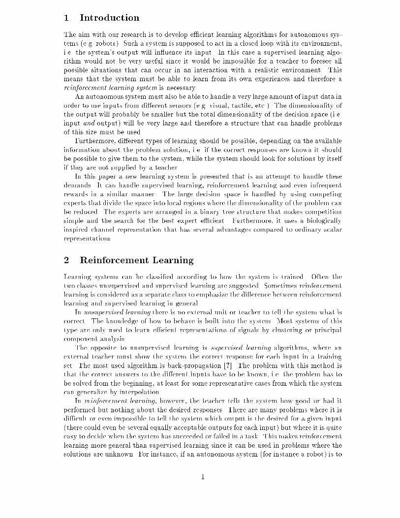
Tv q̂^Figure 1: The reward prediction p for a certain stimulus-response pair (v, q) viewed asa projection onto W in V Q.where ~qi is the correct output fore each output channel supplied by the teacher. Thismeans for the whole system that a matrix W is trained so that a correct output vector isgenerated as q =Wv: (4)In reinforcement learning, however, the correct output is not known and the onlyfeedback is a scalar r that is a measure of the performance of the system. But the rewardsignal is a function of the stimuli vector v and the response vector q, at leastfor anenvironment that is not completely stochastic. If this function can be represented in thesystem, then the best response for each stimulus can be found.4.1 Learning the Reward FunctionIf the reward function is continuous we can approximate it in some interval with a linearfunction of the outer product between the normalized input- and output vectors. Thisapproximation will be used as a prediction p of the reward and is calculated asp = hW j q̂v̂T i; (5)where h� j �i denotes the scalar product, see �gure 1. The space V Q will be calledthe decision space. The normalization implies that the algorithm does not di�er betweeninput vectors with the same orientation but of di�erent length. This is however not aproblem if the channel representation described in section 3 is used. In fact any vector vin an (n�1)-dimensional vector space can be mapped into the orientation of a unit-lengthvector in an n-dimensional space [?].NowWcan be trained in the same manner as in supervised learning but with the aimto minimize the error function � = jr� pj2: (6)Let each triple (v;q; r) of stimulus, response, and reward denote an experience. Con-sider a system that has learned a number of experiences. How should a proper responsebe chosen by the system? The prediction p in equation 5 can be rewritten asp = q̂TWv̂ = hq̂ jWv̂i: (7)The choice of q̂ that gives the highest predicted reward is obviously the q̂ that lies in thesame direction asWv. Now, if p is a good prediction of the reward r for a certain stimulusv that choice of q̂ would be the one that gives the best reward. An obvious choise of theresponse q is then q =Wv: (8)4

This equation together with equation 7 gives the prediction as a function of the stimulusvector, i.e. p = jWv̂j: (See appendix ??.) (9)4.2 The Learning AlgorithmThe training of the matrixW is a very simple algorithm. For a certain experience (v;q; r)the prediction p should in the optimal case equal r. This means that the aim is to minimizethe error in equation 6. The desired weight matrix W0 would yield a predictionp0 = r = hW0 j q̂v̂T i: (10)The direction to search forW0 can be found by calculating the derivative of � with respectto W. From equations 6 and 7 we get the error� = jr� hW j q̂v̂T ij2 (11)and the derivative becomes d�dW = 2(r� p)q̂v̂T : (12)This means that W0 can be obtained by changing W a certain amount a in the directionq̂v̂T , i.e. W0 =W + aq̂v̂T : (13)Equation 10 now gives thatr = p+ a(v̂T v̂) (See appendix??.) (14)which gives a = r � p: (15)To make the learning procedure stable, it is common to take only a small step in thegradient direction. The update rule therefore becomesW0 =W + �(r � p)q̂v̂T (16)where � is a \learning speed factor" (0 < � � 1).4.3 BootstrappingIn the beginning, the system su�ers from a more or less total lack of knowledge of whatresponses give high rewards. This is simply due to the fact that the system may neverhave tried a good response for the present stimulus. The only thing for the system to doin these cases is to generate random output and use the following reward to increase itsknowledge about the problem. This is a kind of bootstrapping mechanism and a standardprocedure in reinforcement learning.The simplest way to produce this behaviour is to add a noise to the output signal.The noise should be large in the beginning when the system has poor knowledge aboutthe problem and should decrease as the knowledge increases. The trivial way to do thiswould be to let the noise level be a monotonically decreasing function of time. A moresophisticated method is to use the predicted reward to decide the noise level. This seemslike a more natural way for the system to work. If the system predicts a high reward,it should mean that the system is rather sure of how to generate a good response and,opposite, if it predicts a low reward this should mean that the response is not very reliable.5

Consequently, a high predicted reward should give a low noise level and a low predictionshould give a high noise level.There are at least two obvious advantages with this approach compared to the timedependent noise. The �rst is that the noise decreasing rate does not have to be predeter-mined, but will be dependent on the problem. The second is that the noise level can bedi�erent for di�erent stimuli, since the system at a given instance probably have di�erentamounts of knowledge about di�erent parts of the problem space.4.4 Similarities to TD-methodsThe description above of the learning algorithm assumed a reward signal as a feedbackto the system for each single decision (i.e. stimulus-response pair). This is, however, notnecessary. Since the system produces a prediction of the following reward this predictioncan be used to produce an internal reward signal in a similar way as in the TD-methodsdescribed in section 2.1. This is simply done by using the next prediction as a rewardsignal when an external reward is lacking. In other wordsr̂ = ( r r > 0 p[t+ 1] r = 0 (17)where r̂ is the internal reward that replaces the external reward r in the algorithm describedabove, p[t+1] is the next predicted reward, and is a prediction decay factor (0 < � 1)that makes the predicted reward decay as the distance from the actual rewarded stateincreases. This means that the system can handle dynamic problems with infrequentreward signals.In fact, this system is more suited to use TD-methods than the earlier methods men-tioned in section 2.1 since those systems had to use a separate subsystem to calculate thepredicted reward. With the algorithm suggested here, this prediction is calculated by thesame system as the response.4.5 Competitive Reinforcement LearningIn a reinforcement learning system there is a problem with the limited feedback. Whenthe system receives the reward (or critic) from the teacher it can be di�cult for the systemto decide what part or parts of the system that is responsible for the rewarded action.This is called the structural credit assignment problem.One way to deal with the structural credit assignment problem is to divide the wholesystem into several subsystems and for each timestep let one of the subsystems decidethe response of the whole system. That subsystem is then the one that takes the creditor blame when receiving the feedback from the teacher. This is similar to the compet-ing experts presented by Jacobs, Jordan, Nowland, and Hinton [?] but here used in areinforcement learning system.Now, how should the system select which of the subsystems that should generatethe response? Since each subsystem calculates not only a potential response but also aprediction of the following reward the subsystem with the highest predicted reward shouldbe chosen.It is not certain that one of the subsystems will become the best for all possiblestimuli. On the contrary, if di�erent subsystems specializes on di�erent parts of theproblem they would together be able to solve a more complicated problem than eachsubsystem itself could solve. This implies that a rather complicated stimuli-responsefunction could be implemented and learned by a su�ciently large number of rather simple6

p

u

Three different subsystemsFigure 2: The global (thick line) and local (thin lines) reward prediction functions.computing units if the units can predict their performance for each stimulus. The total(global) reward prediction function will then be the maximum of the subsystems (local)prediction functions as showed in �gure 2If several systems of the kind described in section 4.2 are used as subsystems in alarger system the subsystem with the highest reward prediction is chosen to generate theresponse. When the reward signal is received it is then the selected subsystem's weightmatrix Wi that is modi�ed according to equation 16. If an internal reward signal is usedto handle infrequent rewards as described in section 4.4 the next predicted reward (p[t+1]in equation 17) is the prediction made by the subsystem that is the \winner" at t+ 1, i.e.the maximum of the predicted rewards. This may not be the same subsystem that usesthe prediction as internal reward to update its weight matrix, but that does not changethe theory since it is the global prediction function that is to be learned by the system.5 The TreeOne way to arrange the competing subsystems is to use a binary tree structure (see �gure3). This structure has several advantages. An obvious advantage is that if a large numberof subsystems is used the search time to �nd the winner will be of order O(log2 n) wheren is the number of experts, while it will be of order O(n) to search in a list of experts.Another feature is that the subdivision of the decision space will be simple since only twosubsystems will compete in each node.5.1 Generating responsesIn section 4 we described the basic functions (i.e. response generation and calculationof predicted reward) of one subsystem or node as it will be called when used in a treestructure. Here we will discuss some issues in the response generation that are dependentor caused by the tree architecture. We will consider a �xed tree that is already adapted tothe solution of the problem. The adaptive growing of the tree will be described in section5.2. 7

W

W W

W

W0

01 02

011 012

WW W

W

W

0 01

02012

011

W

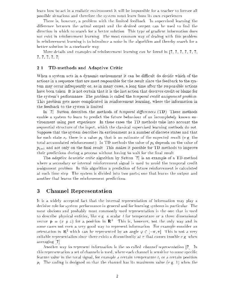
Figure 3: Left: An abstract illustration of a binary tree. Right: A geometric illustrationof the weight matrices in a tree structure (representing three linear functions). Split nodesare marked with a dot (�).Consider the tree in �gure 3. The root node is denoted byW0 and its two childrenW01and W02 respectively and so on. A node without children will be called a leaf node. Theweight matrixW used in a node will be the sum of all matrices from the root to that node.In �gure 3 node 012, for example, will use the weight matrixW =W0+W01+W012. Twonodes with the same father will be called brothers. Two brothers always have oppositedirections since their father lies in the \center of mass" of the brothers (as will be furtherexplained in section 5.2).Now, consider a tree with the two solutions WA =W0+W01 and WB =W0+W02.An input vector v can generate one of the two output vectors qA and qB asqA =WAv = (W0 +W01)v =W0v+W01v = q0 +W01v (18)and qB =WBv = (W0 +W02)v =W0v+W02v = q0 +W02v (19)respectively, where q0 is the solution of the root node. Since W01 and W02 will be ofopposite directions we can write W02 = ��W01, where � is a positive factor, and henceequation 19 can be written as qB = q0 � �W01v: (20)Adding equations 18 and 20 givesq0 = qA + qB � (1� �)W01v2 (21)Now, if WA and WB have equal masses (i.e. the solutions are equally good and equallycommon) then � = 1 and q0 = qA + qB2 ; (22)i.e. q0 will be the average of the two output vectors. IfWA is better or more common (i.e.more likely a priori to appear) than WB then � > 1 (W0 is closer to WA) and q0 willapproach qA. Equation 18 also implies that the response can be generated in a hierarchicalmanner starting with the coarse and global solution of of the root and then re�ning theresponse gradually by just adding to the present output vector the new vectors that are8

P1

1 2p − p

1Figure 4: Illustration of equation 23 for two di�erent cases of �i and ni. The black lineshows a case where the variation is smaller and/or the number of data is larger than inthe case shown by the broken line.generated when traversing the tree. In this way an approximate solution can be generatedvery fast since this solution don't have to wait until the best leaf node is found.The climbing of the tree in search of the best leaf node can be described as a recursiveprocedure.1. Start with the root node: W =W02. Let the current matrix be the father: Wf =W3. Select one of the children [Wf1;Wf2] as winner.4. Add the winner to the father: W =Wf +Wf;winner5. If W is not a leaf node goto 2.6. Generate response: q =Wv.This scheme does not describe the hierarchical response generation mentioned above. Thisis however easily implemented by moving the response generating step into the loop andadding each new output vector to the previous.Now, how should the winner be selected? Well, the most obvious way is to always selectthe child with the highest prediction p. This could, however, cause some problems. Ofreasons explained in section 5.2 the winner will be selected in a probabilistic way. Considertwo children with predictions p1 and p2 respectively. The probability P1 of selecting child1 as winner is P1 = 12 2664erf 0BB@ p1 � p2r�2highnhigh + �2lownlow 1CCA+ 13775 ; (23)Where �high and �low are the variances of the rewards for the choice of the child withhighest prediction and the lowest prediction respectively. nhigh and nlow are the samplesizes of these estimates. When the two predictions are equal the probability for each childto win is 0.5 (see �gure 4). When the variances decreases and the sample sizes increasesthe signi�cance increases in the hypothesis that it is better to chose the node with thehighest prediction as winner than to chose at random. This leads to a sharpening of theerror function and a decrease in the probability of selecting 'wrong' child. This function issimilar to the test of hypothesis on the means of two normal distributions using the pairedt-test i statistics. Here we have used the normal distribution instead of the t-distribution1to be able to use the error function.1The e�ect of this simpli�cation is probably not important since both distributions are unimodal andsymmetric with their maximum at the same point. The exact shape of the distribution is of less importance.9

m m

WW

W

WW12

f

f

12

∆∆

Figure 5: A geometric illustration of the update vectors of a father node and its two childnodes.5.2 Growing the treeSince the size of the tree in general can not bee known in advance we will have to startwith a single node and grow the tree until a satisfying solution is obtained. Hence, westart the learning by trying to solve the problem with a single linear function. This nodewill now try to approximate the optimal function as good as possible. If this solution isnot good enough (i.e. a low average reward is obtained) the node will be split. To �ndout when the node has converged to a solution (optimal or not optimal) a measure ofconsistency of the changes of W is calculated asc = ����� Pk k�WkPk j k�Wkj����� ; (24)where f : 0 < � 1g is the decay factor that makes the measure more sensitive to recentchanges than older ones. These sums are accumulated continuously during the learningprocess. Note that the consistency measure is normalized so that it does not depend uponthe step size in the learning algorithm.Now, if a node is split two new nodes will be created, each with a new weight matrix.The nodes will be selected with a probability that depends on the predicted reward. (Seeequation 23). Consider the case where the problem can be solved with two linear models.The solution developed by the �rst node (the root) will converge to an interpolation ofthe two linear models. This solution will be in between the two optimal solutions in thedecision space (V Q). If the node is split into two child nodes, they will �nd theirsolutions on each side of the father's solution. If the child nodes start in the same positionas their father in the decision space (i.e. they are initialized with zeros) the competitionwill be very simple. As soon as one child becomes closer to one solution the other childwill be closer to the other solution.The mass m of a node is de�ned as the mean reward obtained by that node over alldecisions made by that node or its brother, i.e. a node that often looses in the competitionwith its brother will get a low mass (even if it gets high rewards when it does win). Themass of a node will indicate the nodes share of the total success of itself and its brother.This means that the masses of a winner node and its brother are updated asmwinner :=mwinner + (r�mwinner) (25)and mloser :=mloser + (0�mloser) = (1� )mloser (26)10

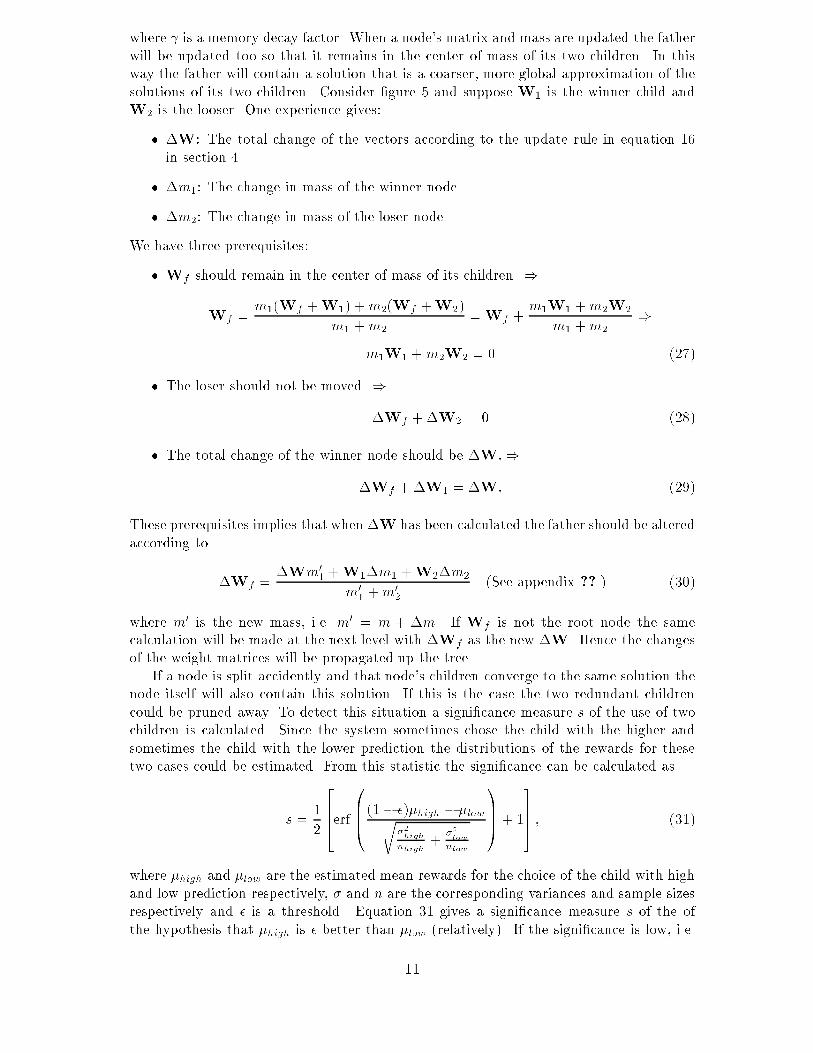
where is a memory decay factor. When a node's matrix and mass are updated the fatherwill be updated too so that it remains in the center of mass of its two children. In thisway the father will contain a solution that is a coarser, more global approximation of thesolutions of its two children. Consider �gure 5 and suppose W1 is the winner child andW2 is the looser. One experience gives:� �W: The total change of the vectors according to the update rule in equation 16in section 4.� �m1: The change in mass of the winner node� �m2: The change in mass of the loser nodeWe have three prerequisites:� Wf should remain in the center of mass of its children. )Wf = m1(Wf +W1) +m2(Wf +W2)m1 +m2 =Wf + m1W1 +m2W2m1 +m2 )m1W1 +m2W2 = 0 (27)� The loser should not be moved. )�Wf +�W2 = 0 (28)� The total change of the winner node should be �W:)�Wf +�W1 = �W: (29)These prerequisites implies that when �W has been calculated the father should be alteredaccording to �Wf = �Wm01 +W1�m1 +W2�m2m01 +m02 (See appendix ??.) (30)where m0 is the new mass, i.e. m0 = m + �m. If Wf is not the root node the samecalculation will be made at the next level with �Wf as the new �W. Hence the changesof the weight matrices will be propagated up the tree.If a node is split accidently and that node's children converge to the same solution thenode itself will also contain this solution. If this is the case the two redundant childrencould be pruned away. To detect this situation a signi�cance measure s of the use of twochildren is calculated. Since the system sometimes chose the child with the higher andsometimes the child with the lower prediction the distributions of the rewards for thesetwo cases could be estimated. From this statistic the signi�cance can be calculated ass = 12 2664erf 0BB@ (1� �)�high � �lowr�2highnhigh + �2lownlow 1CCA+ 13775 ; (31)where �high and �low are the estimated mean rewards for the choice of the child with highand low prediction respectively, � and n are the corresponding variances and sample sizesrespectively and � is a threshold. Equation 31 gives a signi�cance measure s of the ofthe hypothesis that �high is � better than �low (relatively). If the signi�cance is low, i.e.11

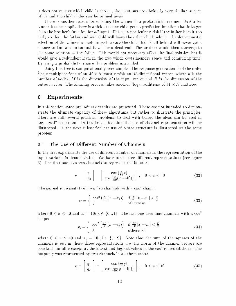
it does not matter which child is chosen, the solutions are obviously very similar to eachother and the child nodes can be pruned away.There is another reason for selecting the winner in a probabilistic manner. Just aftera node has been split there is a risk that one child gets a prediction function that is largerthan the brother's function for all input. This is in particular a risk if the father is split tooearly so that the father and one child will leave the other child behind. If a deterministicselection of the winner is made in such a case the child that is left behind will never get achance to �nd a solution and it will be a dead end. The brother would then converge tothe same solution as the father. This would not necessary a�ect the �nal solution but itwould give a redundant level in the tree which costs memory space and computing time.By using a probabilistic choice this problem is avoided.Using this tree is computationally very simple. The response generation is of the order2log n multiplications of an M �N matrix with an M -dimensional vector, where n is thenumber of nodes, M is the dimension of the input vector and N is the dimension of theoutput vector. The learning process takes another 2logn additions of M �N matrices.6 ExperimentsIn this section some preliminary results are presented. These are not intended to demon-strate the ultimate capacity of these algorithms but rather to illustrate the principles.There are still several practical problems to deal with before the ideas can be used inany \real" situations. In the �rst subsection the use of channel representation will beillustrated. In the next subsection the use of a tree structure is illustrated on the sameproblem.6.1 The Use of Di�erent Number of ChannelsIn the �rst experiments the use of di�erent number of channels in the representation of theinput variable is demonstrated. We have used three di�erent representations (see �gure6). The �rst one uses two channels to represent the input x:v = " v1v2 # = " cos � �80x�cos � �80(x� 40)� # ; 0 � x � 40 (32)The second representation uses �ve channels with a cos2 shape:vi = ( cos2 � �30 (x� xi)� if �30 jx� xij < �20 otherwise (33)where 0 � x � 40 and xi = 10i; i 2 f0:::4g. The last one uses nine channels with a cos2shape: vi = ( cos2 �2�30 (x� xi)� if 2�30 jx� xij < �20 otherwise (34)where 0 � x � 40 and xi = 10i; i 2 f0:::9g. Note that the sum of the squares of thechannels is one in these three representations, i.e. the norm of the channel vectors areconstant, for all x except at the lowest and highest values in the cos2 representations. Theoutput y was represented by two channels in all three cases:q = " q1q2 # = " cos � �80y�cos � �80(y � 40)� # ; 0 � y � 40 (35)12

0 5 10 15 20 25 30 35 400

0.5

1

0 5 10 15 20 25 30 35 400

0.5

1

0 5 10 15 20 25 30 35 400

0.5

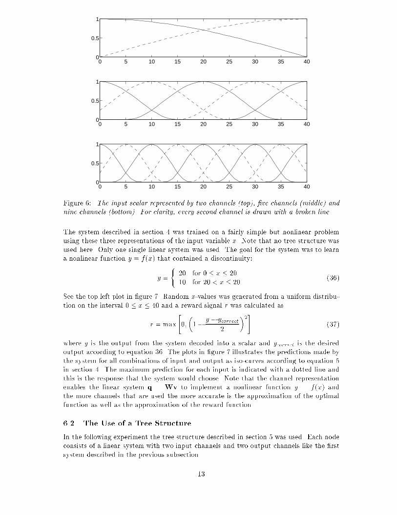
1Figure 6: The input scalar represented by two channels (top), �ve channels (middle) andnine channels (bottom). For clarity, every second channel is drawn with a broken line.The system described in section 4 was trained on a fairly simple but nonlinear problemusing these three representations of the input variable x. Note that no tree structure wasused here. Only one single linear system was used. The goal for the system was to learna nonlinear function y = f(x) that contained a discontinuity:y = ( 20 for 0 � x � 2010 for 20 < x � 20 (36)See the top left plot in �gure 7. Random x-values was generated from a uniform distribu-tion on the interval 0 � x � 40 and a reward signal r was calculated asr = max"0;�1� y � ycorrect2 �2# (37)where y is the output from the system decoded into a scalar and ycorrect is the desiredoutput according to equation 36. The plots in �gure 7 illustrates the predictions made bythe system for all combinations of input and output as iso-curves according to equation 5in section 4. The maximum prediction for each input is indicated with a dotted line andthis is the response that the system would choose. Note that the channel representationenables the linear system q = Wv to implement a nonlinear function y = f(x) andthe more channels that are used the more accurate is the approximation of the optimalfunction as well as the approximation of the reward function.6.2 The Use of a Tree StructureIn the following experiment the tree structure described in section 5 was used. Each nodeconsists of a linear system with two input channels and two output channels like the �rstsystem described in the previous subsection.13

0 5 10 15 20 25 30 35 400

5

10

15

20

25

30

35

40

5 10 15 20 25 30 35 40

5

10

15

20

25

30

35

40

5 10 15 20 25 30 35 40

5

10

15

20

25

30

35

40

5 10 15 20 25 30 35 40

5

10

15

20

25

30

35

40

Figure 7: The top left �gure displays the optimal function. The other three �gures illus-trates the predictions as iso-curves with the maximum prediction at the dotted line for two,�ve and nine channels in top right, bottom left and bottom right image respectively.14

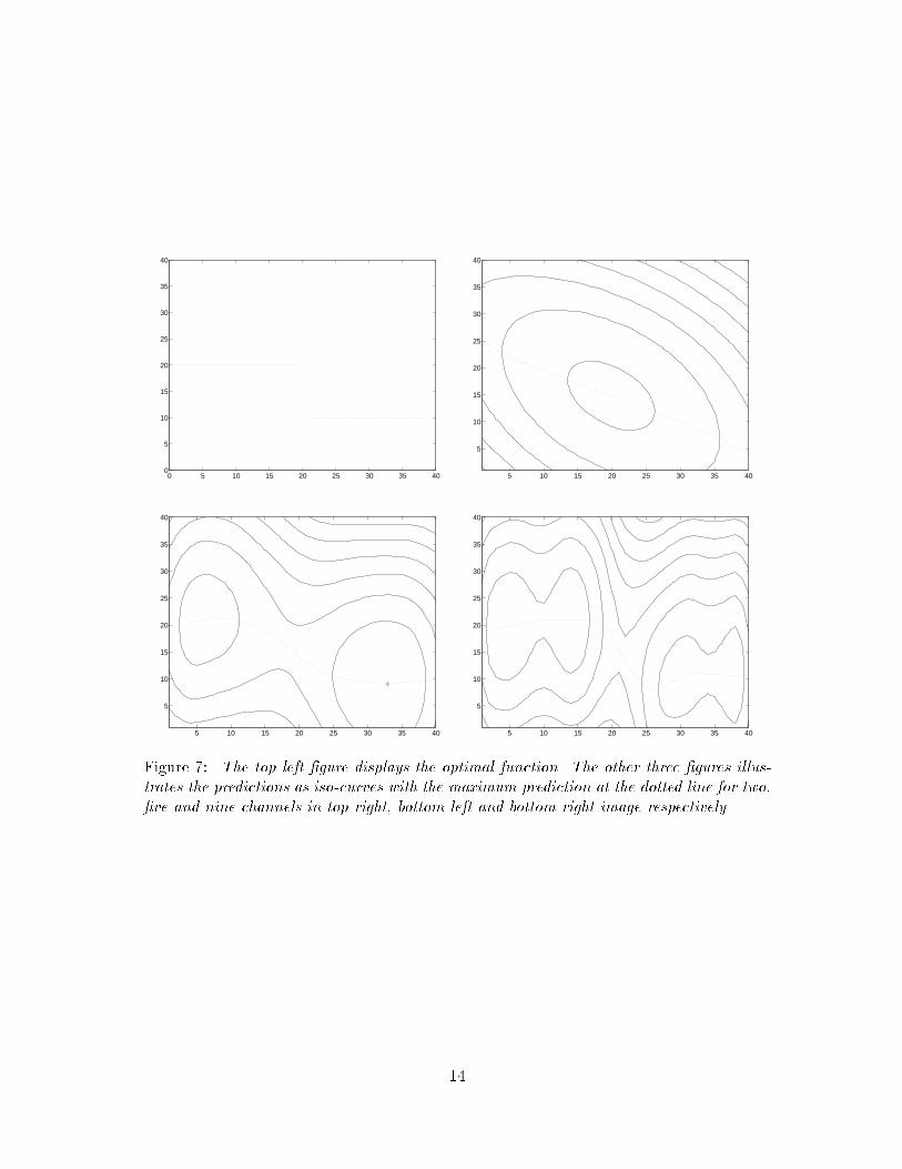
The system was trained on the same problem as in the previous subsection (equation36). The input variable was generated in the same way as above and the reward functionwas the same as in equation 37. Each iteration consists of one input, one output and areward signal. The result is plotted in �gure ??. It is obvious that this problem can besolved with a two-level tree and that is what the algorithm converged to. The discontinuityexplains the fact that this solution with only two channels is better than the solutions inthe previous experiments with more channels but with only one level.5 10 15 20 25 30 35 40

5

10

15

20

25

30

35

40

Figure 8: The result using a tree structure. The predictions are illustrated by iso-curveswith the maximum prediction at the dotted line. The optimal function is drawn as a solidline.6.3 The XOR-problemThe aim of this experiment is to demonstrate the use of the tree structure in a problemthat is impossible to solve even approximately on one single level, no matter how manychannel are fused. The problem is to implement a function similar to the Boolean XOR-function. The input consists of two parameters, x1 and x2, that each are represented bynine channels. The two channel vectors are concatenated to form an input channel vectorv with 18 channels.The function the system is to learn isy = ( 1 if (x1 > 0:5 AND x2 � 0:5) OR (x1 � 0:5 AND x2 > 0:5)0 otherwise (38)wich is illustrated left in �gure ??.7 DiscussionA new reinforcement learning algorithm has been presented that take advantage of thechannel representation. It can use simple linear models to implement non-linear functions.Since it generates predictions of the reward signals it can also be used for handling delayedrewards like the TD-methods.A dynamic binary tree structure for this type of reinforcement learning systems hasbeen developed. In this structure the nodes are competing experts that specialize onregions of the decision space where the function can be described in a simple (i.e. linear)way. The tree is dynamic in the sense that it continuously tests split- and prune criteria15

00.2

0.40.6

0.81

0

0.2

0.4

0.6

0.8

1−1

0

1

2

3

x1x2

y

00.2

0.40.6

0.81

0

0.2

0.4

0.6

0.8

1−1

0

1

2

3

x1x2

yFigure 9: Left: The correct XOR-function. Right: The result after 4000 itterations.and therefore it does not have a predetermined size. It can also have di�erent depths indi�erent parts of the decision space depending on the local complexity of the solution.We argue that reinforcement learning together with a dynamic tree structure willbe useful in the design of a learning autonomous system. Some experiments have beenpresented to illustrate the ideas applied on a simple but illustrative problem. There are,however, some di�culties left to solve before this method can be used on more complexproblems. We will end this report by describing a few problems more explicitly.7.1 Breakpoint InstabilityA function as the one described in �gure ?? could theoretically be represented exactlyby a two level tree with x represented by two channels. One reason that this solution inpractice does no yiel perfect resultes is due to the instability of the breakpoint betweenthe two child nodes. This problem is related to the fact that the shape of the predictionfunction is �x when only two channels are used. Hence, while this function is su�cient fora subsystem to select a best response for a certain stimulus, it is not completely reliablewhen compared to a prediction function of another subsystem.The reward prediction p as a function of the input variable x can, simpli�ed, bedescribed as a quadratic function in this case. The breakpoint x between two competingmodels can then be described bya� (x� xa)2 = b� (x� xb)2: (39)See �gure ?? This gives the following relation for the breakpoint:x = b� a+ x2a � x2b2(xa � xb) (40)If this equation is di�erentiated with respect to a we get@x@a = � 12(xa � xb) : (41)This indicates that the position of the breakpoint is very unstable when the centers ofthe reward functions lie close to each other. This is the case short after a split when thetwo child nodes contains almost the same solution. The factors a and b in this discussionrepresents the norm of the matrices WA and WB.The easiest way to deal with this problem is to use more channels to represent theinput parameters. 16

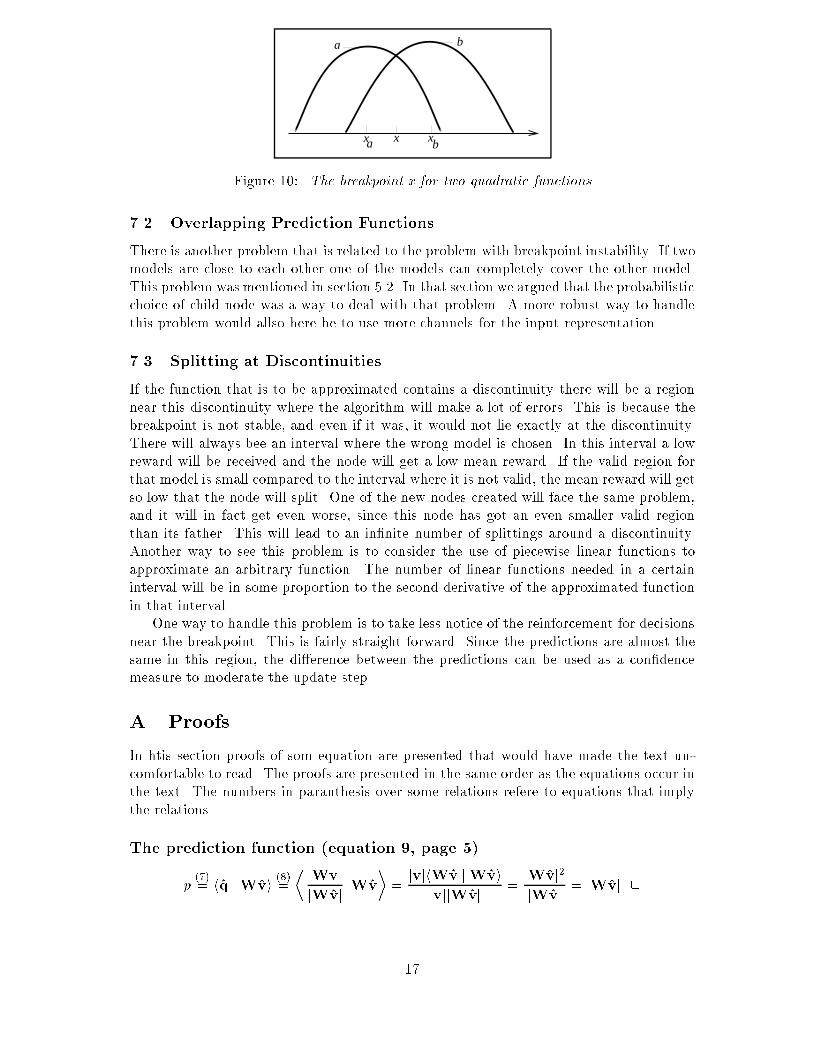
a b

x xxa bFigure 10: The breakpoint x for two quadratic functions7.2 Overlapping Prediction FunctionsThere is another problem that is related to the problem with breakpoint instability. If twomodels are close to each other one of the models can completely cover the other model.This problem was mentioned in section 5.2. In that section we argued that the probabilisticchoice of child node was a way to deal with that problem. A more robust way to handlethis problem would allso here be to use more channels for the input representation.7.3 Splitting at DiscontinuitiesIf the function that is to be approximated contains a discontinuity there will be a regionnear this discontinuity where the algorithm will make a lot of errors. This is because thebreakpoint is not stable, and even if it was, it would not lie exactly at the discontinuity.There will always bee an interval where the wrong model is chosen. In this interval a lowreward will be received and the node will get a low mean reward. If the valid region forthat model is small compared to the interval where it is not valid, the mean reward will getso low that the node will split. One of the new nodes created will face the same problem,and it will in fact get even worse, since this node has got an even smaller valid regionthan its father. This will lead to an in�nite number of splittings around a discontinuity.Another way to see this problem is to consider the use of piecewise linear functions toapproximate an arbitrary function. The number of linear functions needed in a certaininterval will be in some proportion to the second derivative of the approximated functionin that interval.One way to handle this problem is to take less notice of the reinforcement for decisionsnear the breakpoint. This is fairly straight forward. Since the predictions are almost thesame in this region, the di�erence between the predictions can be used as a con�dencemeasure to moderate the update step.A ProofsIn htis section proofs of som equation are presented that would have made the text un-comfortable to read. The proofs are presented in the same order as the equations occur inthe text. The numbers in paranthesis over some relations refere to equations that implythe relations.The prediction function (equation 9, page 5)p (7)= hq̂ jWv̂i (8)= � WvjWv̂j����Wv̂� = jvjhWv̂ jWv̂ijvjjWv̂j = jWv̂j2jWv̂j = jWv̂j 217

Derivation of the update rule (equation 14, page 5)r (10;13)= hW + aq̂v̂T j q̂v̂T i == hW j q̂v̂T i+ ahq̂v̂T j q̂v̂T i == p+ a(q̂T q̂v̂T v̂) == p+ a(v̂T v̂) 2The change of the father node (equation 30, page 11)After the update of mi and Wi we get(m1 +�m1)(W1 +�W1) + (m2 +�m2)(W2 +�W2) (27)= 0and this equation together with equations 27, 28 and 29 gives(m1 + �m1)(W1 + �W��Wf ) + (m2 + �m2)(W2 ��Wf) = 0:This leads to �Wf(m1 +�m1 +m2 +�m2) == (W1 + �W)(m1+ �m1) +W2(m2 +�m2) == W1m1 +W2m2| {z }=0 (27) +�W(m1 +�m1) +W1�m1 +W2�m2which with the substitution m0 = m+ �m gives the result:�Wf = �Wm01 +W1�m1 +W2�m2m01 +m02 2References[1] D. H. Ballard. Vision, Brain, and Cooperative Computation, chapter Cortical Con-nections and Parallel Processing: Structure and Function. MIT Press, 1987. M. A.Arbib and A. R. Hanson, Eds.[2] A. G. Barto, R. S. Sutton, and C. W. Anderson. Neuronlike adaptive elements thatcan solve di�cult learning control problems. IEEE Trans. on Systems, Man, andCybernetics, SMC-13(8):834{846, 1983.[3] M. Borga and T. Carlsson. A Survey of Current Techniques for Reinforcement Learn-ing. Report LiTH-ISY-I-1391, Computer Vision Laboratory, S{581 83 Link�oping,Sweden, 1992.[4] T. Denoeux and R. Lengell�e. Initializing back propagation networks with prototypes.Neural Networks, 6(3):351{363, 1993.[5] D. J. Field. What is the goal of sensory coding? Neural Computation, 1994. in press.[6] G. H. Granlund. Magnitude representation of features in image analysis. In The6th Scandinavian Conference on Image Analysis, pages 212{219, Oulu, Finland, June1989. 18

[7] V. Gullapalli. A stochastic reinforcement learning algorithm for learning real-valuedfunctions. Neural Networks, 3:671{692, 1990.[8] D. H. Hubel. Eye, Brain and Vision, volume 22 of Scienti�c American Library. W.H. Freeman and Company, 1988.[9] R. A. Jacobs, M. I. Jordan, S. J. Nowlan, and G. E. Hinton. Adaptive mixtures oflocal experts. Neural Computation, 3:79{87, 1991.[10] H. Knutsson. Representing local structure using tensors. In The 6th Scandina-vian Conference on Image Analysis, pages 244{251, Oulu, Finland, June 1989. Re-port LiTH{ISY{I{1019, Computer Vision Laboratory, Link�oping University, Sweden,1989.[11] C-S. Lin and H. Kim. CMAC-based adaptive critic self-learning control. IEEE Trans.on Neural Networks, 2(5):530{533, 1991.[12] J. L. Musgrave and K. A. Loparo. Entropy and outcome classi�cation in reinforcementlearning control. In IEEE Int. Symp. on Intelligent Control, pages 108{114, 1989.[13] K. Nordberg, G. Granlund, and H. Knutsson. Representation and learning of invari-ance. Report LiTH-ISY-I-1552, Computer Vision Laboratory, S{581 83 Link�oping,Sweden, 1994.[14] D. E. Rumelhart, G. E. Hinton, and R. J. Williams. Learning representations byback-propagating errors. Nature, 323:533{536, 1986.[15] Robert E. Smith and David E. Goldberg. Reinforcement learning with classi�er sys-tems. Proceedings. AI, Simulation and Planning in High Autonomy Systems, 6:284{192, 1990.[16] R. S. Sutton. Temporal credit assignment in reinforcement learning. PhD thesis,University of Massachusetts, Amherst, MA., 1984.[17] R. S. Sutton. Learning to predict by the methods of temporal di�erences. MachineLearning, 3:9{44, 1988.[18] Chris Watkins. Learning from delayed rewards. PhD thesis, Cambridge University,1989.[19] P. J. Werbos. Consistency of HDP applied to a simple reinforcement learning problem.Neural Networks, 3:179{189, 1990.[20] S. D. Whitehead, R. S. Sutton, and D. H. Ballard. Advances in reinforcement learn-ing and their implications for intelligent control. Proceedings of the 5th IEEE Int.Symposium on Intelligent Control, 2:1289{1297, 1990.19