imperfect competition

C H A P T E RFIFTEEN Imperfect Competition

This chapter discusses oligopoly markets, falling between the extremes of perfect compe-tition and monopoly.

Oligopolies raise the possibility of strategic interaction among firms. To analyze this stra-tegic interaction rigorously, we will apply the concepts from game theory that were intro-duced in Chapter 8. Our game-theoretic analysis will show that small changes in detailsconcerning the variables firms choose, the timing of their moves, or their information aboutmarket conditions or rival actions can have a dramatic effect on market outcomes. The firsthalf of the chapter deals with short-term decisions such as pricing and output, and thesecond half covers longer-term decisions such as investment, advertising, and entry.

Short-Run Decisions: PricingAnd OutputIt is difficult to predict exactly the possible outcomes for price and output when there arefew firms; prices depend on how aggressively firms compete, which in turn depends onwhich strategic variables firms choose, how much information firms have about rivals,and how often firms interact with each other in the market.

For example, consider the Bertrand game studied in the next section. The gameinvolves two identical firms choosing prices simultaneously for their identical products intheir one meeting in the market. The Bertrand game has a Nash equilibrium at point Cin Figure 15.1. Even though there may be only two firms in the market, in this equilib-rium they behave as though they were perfectly competitive, setting price equal to mar-ginal cost and earning zero profit. We will discuss whether the Bertrand game is arealistic depiction of actual firm behavior, but an analysis of the model shows that it ispossible to think up rigorous game-theoretic models in which one extreme—the competi-tive outcome—can emerge in concentrated markets with few firms.

At the other extreme, as indicated by point M in Figure 15.1, firms as a group may actas a cartel, recognizing that they can affect price and coordinate their decisions. Indeed,they may be able to act as a perfect cartel and achieve the highest possible profits—namely, the profit a monopoly would earn in the market. One way to maintain a cartel isto bind firms with explicit pricing rules. Such explicit pricing rules are often prohibitedby antitrust law. But firms need not resort to explicit pricing rules if they interact on themarket repeatedly; they can collude tacitly. High collusive prices can be maintained with

D E F I N I T I O N Oligopoly. A market with relatively few firms but more than one.

531

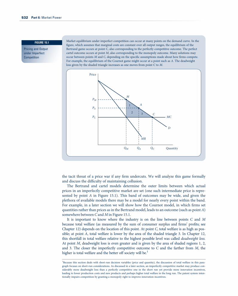
the tacit threat of a price war if any firm undercuts. We will analyze this game formallyand discuss the difficulty of maintaining collusion.

The Bertrand and cartel models determine the outer limits between which actualprices in an imperfectly competitive market are set (one such intermediate price is repre-sented by point A in Figure 15.1). This band of outcomes may be wide, and given theplethora of available models there may be a model for nearly every point within the band.For example, in a later section we will show how the Cournot model, in which firms setquantities rather than prices as in the Bertrandmodel, leads to an outcome (such as pointA)somewhere betweenC andM in Figure 15.1.

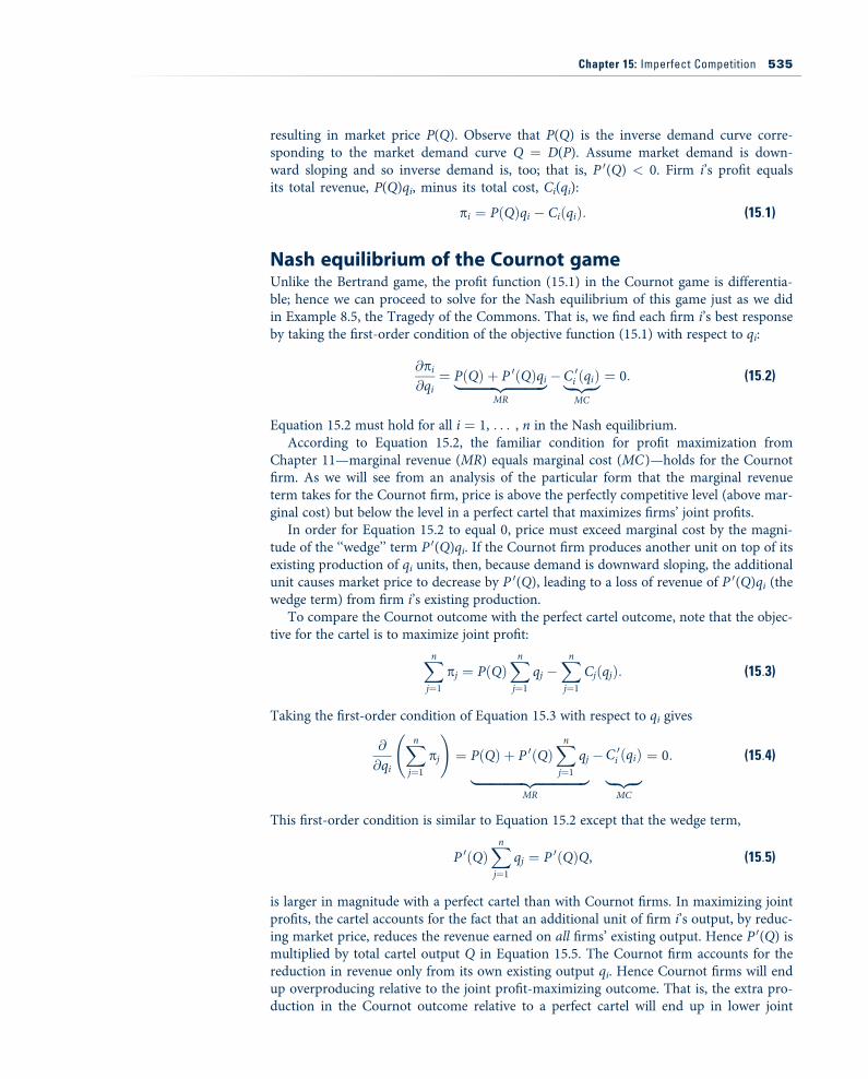
It is important to know where the industry is on the line between points C and Mbecause total welfare (as measured by the sum of consumer surplus and firms’ profits; seeChapter 12) depends on the location of this point. At point C, total welfare is as high as pos-sible; at point A, total welfare is lower by the area of the shaded triangle 3. In Chapter 12,this shortfall in total welfare relative to the highest possible level was called deadweight loss.At point M, deadweight loss is even greater and is given by the area of shaded regions 1, 2,and 3. The closer the imperfectly competitive outcome to C and the farther from M, thehigher is total welfare and the better off society will be.1

Market equilibrium under imperfect competition can occur at many points on the demand curve. In thefigure, which assumes that marginal costs are constant over all output ranges, the equilibrium of theBertrand game occurs at point C, also corresponding to the perfectly competitive outcome. The perfectcartel outcome occurs at point M, also corresponding to the monopoly outcome. Many solutions mayoccur between points M and C, depending on the specific assumptions made about how firms compete.For example, the equilibrium of the Cournot game might occur at a point such as A. The deadweightloss given by the shaded triangle increases as one moves from point C to M.

Price

PM

PA

PC

QM QA QC

MR

MCC

A

M

Quantity

D

1

2 3

1Because this section deals with short-run decision variables (price and quantity), the discussion of total welfare in this para-graph focuses on short-run considerations. As discussed in a later section, an imperfectly competitive market may produce con-siderably more deadweight loss than a perfectly competitive one in the short run yet provide more innovation incentives,leading to lower production costs and new products and perhaps higher total welfare in the long run. The patent system inten-tionally impairs competition by granting a monopoly right to improve innovation incentives.

FIGURE 15.1

Pricing and Outputunder ImperfectCompetition

532 Part 6: Market Power

Bertrand ModelThe Bertrand model is named after the economist who first proposed it.2 The model is agame involving two identical firms, labeled 1 and 2, producing identical products at aconstant marginal cost (and constant average cost) c. The firms choose prices p1 and p2simultaneously in a single period of competition. Because firms’ products are perfect sub-stitutes, all sales go to the firm with the lowest price. Sales are split evenly if p1 ! p2. LetD(p) be market demand.

We will look for the Nash equilibrium. The game has a continuum of actions, as doesExample 8.5 (the Tragedy of the Commons) in Chapter 8. Unlike Example 8.5, we cannotuse calculus to derive best-response functions because the profit functions are not differ-entiable here. Starting from equal prices, if one firm lowers its price by the smallestamount, then its sales and profit would essentially double. We will proceed by first guess-ing what the Nash equilibrium is and then spending some time to verify that our guesswas in fact correct.

Nash equilibrium of the Bertrand gameThe only pure-strategy Nash equilibrium of the Bertrand game is p"1 ! p"2 ! c. That is,the Nash equilibrium involves both firms charging marginal cost. In saying that thisis the only Nash equilibrium, we are making two statements that need to be verified:This outcome is a Nash equilibrium, and there is no other Nash equilibrium.

To verify that this outcome is a Nash equilibrium, we need to show that both firmsare playing a best response to each other—or, in other words, that neither firm has an in-centive to deviate to some other strategy. In equilibrium, firms charge a price equal tomarginal cost, which in turn is equal to average cost. But a price equal to average costmeans firms earn zero profit in equilibrium. Can a firm earn more than the zero it earnsin equilibrium by deviating to some other price? No. If it deviates to a higher price, thenit will make no sales and therefore no profit, not strictly more than in equilibrium. If itdeviates to a lower price, then it will make sales but will be earning a negative margin oneach unit sold because price would be below marginal cost. Thus, the firm would earnnegative profit, less than in equilibrium. Because there is no possible profitable deviationfor the firm, we have succeeded in verifying that both firms’ charging marginal cost is aNash equilibrium.

It is clear that marginal cost pricing is the only pure-strategy Nash equilibrium. Ifprices exceeded marginal cost, the high-price firm would gain by undercutting the otherslightly and capturing all the market demand. More formally, to verify that p"1 ! p"2 ! cis the only Nash equilibrium, we will go one by one through an exhaustive list of casesfor various values of p1, p2, and c, verifying that none besides p1 ! p2 ! c is a Nashequilibrium. To reduce the number of cases, assume firm 1 is the low-price firm—thatis, p l # p2. The same conclusions would be reached taking 2 to be the low-price firm.

There are three exhaustive cases: (i) c > p1, (ii) c < p1, and (iii) c ! p1. Case (i) cannotbe a Nash equilibrium. Firm 1 earns a negative margin pl $ c on every unit it sells, andbecause it makes positive sales, it must earn negative profit. It could earn higher profit bydeviating to a higher price. For example, firm 1 could guarantee itself zero profit by devi-ating to p1 ! c.

Case (ii) cannot be a Nash equilibrium either. At best, firm 2 gets only half of marketdemand (if p1 ! p2) and at worst gets no demand (if p1 < p2). Firm 2 could capture allthe market demand by undercutting firm 1’s price by a tiny amount e. This e could be

2J. Bertrand, ‘‘Theorie Mathematique de la Richess Sociale,’’ Journal de Savants (1883): 499–508.

Chapter 15: Imperfect Competition 533

chosen small enough that market price and total market profit are hardly affected. If p1! p2before the deviation, the deviation would essentially double firm 2’s profit. If pl < p2 beforethe deviation, the deviation would result in firm 2 moving from zero to positive profit.In either case, firm 2’s deviation would be profitable.

Case (iii) includes the subcase of p1 ! p2 ! c, which we saw is a Nash equilibrium.The only remaining subcase in which p1 # p2 is c ! p1 < p2. This subcase cannot be aNash equilibrium: Firm 1 earns zero profit here but could earn positive profit by deviat-ing to a price slightly above c but still below p2.

Although the analysis focused on the game with two firms, it is clear that the sameoutcome would arise for any number of firms n % 2. The Nash equilibrium of the n-firmBertrand game is p"1 ! p"2 ! & & & ! p"n ! c.

Bertrand paradoxThe Nash equilibrium of the Bertrand model is the same as the perfectly competitive out-come. Price is set to marginal cost, and firms earn zero profit. This result—that the Nashequilibrium in the Bertrand model is the same as in perfect competition even thoughthere may be only two firms in the market—is called the Bertrand paradox. It is paradoxi-cal that competition between as few as two firms would be so tough. The Bertrand para-dox is a general result in the sense that we did not specify the marginal cost c or thedemand curve; therefore, the result holds for any c and any downward-sloping demandcurve.

In another sense, the Bertrand paradox is not general; it can be undone by changingvarious of the model’s other assumptions. Each of the next several sections will present adifferent model generated by changing a different one of the Bertrand assumptions. Inthe next section, for example, we will assume that firms choose quantity rather than price,leading to what is called the Cournot game. We will see that firms do not end up chargingmarginal cost and earning zero profit in the Cournot game. In subsequent sections, wewill show that the Bertrand paradox can also be avoided if still other assumptions arechanged: if firms face capacity constraints rather than being able to produce an unlimitedamount at cost c, if products are slightly differentiated rather than being perfect substi-tutes, or if firms engage in repeated interaction rather than one round of competition.

Cournot ModelThe Cournot model, named after the economist who proposed it,3 is similar to the Ber-trand model except that firms are assumed to simultaneously choose quantities ratherthan prices. As we will see, this simple change in strategic variable will lead to a bigchange in implications. Price will be above marginal cost, and firms will earn positiveprofit in the Nash equilibrium of the Cournot game. It is somewhat surprising (but none-theless an important point to keep in mind) that this simple change in choice variablematters in the strategic setting of an oligopoly when it did not matter with a monopoly:The monopolist obtained the same profit-maximizing outcome whether it chose prices orquantities.

We will start with a general version of the Cournot game with n firms indexed byi ! 1, . . . , n. Each firm chooses its output qi of an identical product simultaneously.The outputs are combined into a total industry output Q ! q1 ' q2 ' & & & ' qn,

3A. Cournot, Researches into the Mathematical Principles of the Theory of Wealth, trans. N. T. Bacon (New York: Macmillan,1897). Although the Cournot model appears after Bertrand’s in this chapter, Cournot’s work, originally published in 1838, pre-dates Bertrand’s. Cournot’s work is one of the first formal analyses of strategic behavior in oligopolies, and his solution conceptanticipated Nash equilibrium.


resulting in market price P(Q). Observe that P(Q) is the inverse demand curve corre-sponding to the market demand curve Q ! D(P). Assume market demand is down-ward sloping and so inverse demand is, too; that is, P 0(Q) < 0. Firm i’s profit equalsits total revenue, P(Q)qi, minus its total cost, Ci(qi):

pi ! P(Q)qi $ Ci(qi): (15:1)

Nash equilibrium of the Cournot gameUnlike the Bertrand game, the profit function (15.1) in the Cournot game is differentia-ble; hence we can proceed to solve for the Nash equilibrium of this game just as we didin Example 8.5, the Tragedy of the Commons. That is, we find each firm i’s best responseby taking the first-order condition of the objective function (15.1) with respect to qi:

@pi

@qi! P(Q) ' P 0(Q)qi|!!!!!!!!!!!!{z!!!!!!!!!!!!}

MR

$C 0i (qi)|!!{z!!}MC

! 0: (15:2)

Equation 15.2 must hold for all i ! 1, . . . , n in the Nash equilibrium.According to Equation 15.2, the familiar condition for profit maximization from

Chapter 11—marginal revenue (MR) equals marginal cost (MC)—holds for the Cournotfirm. As we will see from an analysis of the particular form that the marginal revenueterm takes for the Cournot firm, price is above the perfectly competitive level (above mar-ginal cost) but below the level in a perfect cartel that maximizes firms’ joint profits.

In order for Equation 15.2 to equal 0, price must exceed marginal cost by the magni-tude of the ‘‘wedge’’ term P 0(Q)qi. If the Cournot firm produces another unit on top of itsexisting production of qi units, then, because demand is downward sloping, the additionalunit causes market price to decrease by P 0(Q), leading to a loss of revenue of P 0(Q)qi (thewedge term) from firm i’s existing production.

To compare the Cournot outcome with the perfect cartel outcome, note that the objec-tive for the cartel is to maximize joint profit:

Xn

j!1pj ! P(Q)

Xn

j!1qj $

Xn

j!1Cj(qj): (15:3)

Taking the first-order condition of Equation 15.3 with respect to qi gives

@

@qi

Xn

j!1pj

!

! P(Q) ' P 0(Q)Xn

j!1qj

|!!!!!!!!!!!!!!!!{z!!!!!!!!!!!!!!!!}MR

$C 0i (qi)

|!!{z!!}MC

! 0: (15:4)

This first-order condition is similar to Equation 15.2 except that the wedge term,

P 0(Q)Xn

j!1qj ! P 0(Q)Q, (15:5)

is larger in magnitude with a perfect cartel than with Cournot firms. In maximizing jointprofits, the cartel accounts for the fact that an additional unit of firm i’s output, by reduc-ing market price, reduces the revenue earned on all firms’ existing output. Hence P 0(Q) ismultiplied by total cartel output Q in Equation 15.5. The Cournot firm accounts for thereduction in revenue only from its own existing output qi. Hence Cournot firms will endup overproducing relative to the joint profit-maximizing outcome. That is, the extra pro-duction in the Cournot outcome relative to a perfect cartel will end up in lower joint


profit for the firms. What firms would regard as overproduction is good for societybecause it means that the Cournot outcome (point A, referring back to Figure 15.1) willinvolve more total welfare than the perfect cartel outcome (point M in Figure 15.1).

EXAMPLE 15.1 Natural-Spring Duopoly

As a numerical example of some of these ideas, we will consider a case with just two firms andsimple demand and cost functions. Following Cournot’s nineteenth-century example of twonatural springs, we assume that each spring owner has a large supply of (possibly healthful)water and faces the problem of how much to provide the market. A firm’s cost of pumping andbottling qi liters is Ci(qi) ! cqi, implying that marginal costs are a constant c per liter. Inversedemand for spring water is

P(Q) ! a$ Q, (15:6)

where a is the demand intercept (measuring the strength of spring water demand) and Q ! q1 ' q2is total spring water output. We will now examine various models of how this market might operate.

Bertrand model. In the Nash equilibrium of the Bertrand game, the two firms set price equalto marginal cost. Hence market price is P" ! c, total output is Q" ! a $ c, firm profit isp"i ! 0, and total profit for all firms is G" ! 0. For the Bertrand quantity to be positive wemust have a > c, which we will assume throughout the problem.

Cournot model. The solution for the Nash equilibrium follows Example 8.6 closely. Profitsfor the two Cournot firms are

p1 ! P(Q)q1 $ cq1 ! (a$ q1 $ q2 $ c)q1,p2 ! P(Q)q2 $ cq2 ! (a$ q1 $ q2 $ c)q2:

(15:7)

Using the first-order conditions to solve for the best-response functions, we obtain

q1 !a$ q2 $ c

2, q2 !

a$ q1 $ c2

: (15:8)

Solving Equations 15.8 simultaneously yields the Nash equilibrium

q"1 ! q"2 !a$ c3

: (15:9)

Thus, total output is Q" ! (2/3)(a $ c). Substituting total output into the inverse demand curveimplies an equilibrium price of P" ! (a ' 2c)/3. Substituting price and outputs into the profitfunctions (Equations 15.7) implies p"1 ! p"2 ! (1=9)(a$ c)2, so total market profit equalsG" ! p"1 ! p"2 ! (2=9)(a$ c)2.

Perfect cartel. The objective function for a perfect cartel involves joint profits

p1 ' p2 ! (a$ q1 $ q2 $ c)q1 ' (a$ q1 $ q2 $ c)q2: (15:10)

The two first-order conditions for maximizing Equation 15.10 with respect to q1 and q2 are thesame:

@

@q1(p1 ' p2) !

@

@q2(p1 ' p2) ! a$ 2q1 $ 2q2 $ c ! 0: (15:11)

The first-order conditions do not pin down market shares for firms in a perfect cartel becausethey produce identical products at constant marginal cost. But Equation 15.11 does pin down totaloutput: q"1 ' q"2 ! Q" ! (1=2)(a$ c). Substituting total output into inverse demand implies thatthe cartel price is P" ! (1/2)(a ' c). Substituting price and quantities into Equation 15.10 impliesa total cartel profit of G" ! (1/4)(a $ c)2.


Comparison. Moving from the Bertrand model to the Cournot model to a perfect cartel, becausea> c we can show that quantity Q" decreases from a$ c to (2 / 3)(a$ c) to (1 / 2)(a$ c). It can alsobe shown that price P" and industry profit G" increase. For example, if a! 120 and c! 0 (implyingthat inverse demand is P(Q)! 120$ Q and that production is costless), then market quantity is 120with Bertrand competition, 80 with Cournot competition, and 60 with a perfect cartel. Priceincreases from 0 to 40 to 60 across the cases, and industry profit increases from 0 to 3,200 to 3,600.

QUERY: In a perfect cartel, do firms play a best response to each other’s quantities? If not, inwhich direction would they like to change their outputs? What does this say about the stabilityof cartels?

EXAMPLE 15.2 Cournot Best-Response Diagrams

Continuing with the natural-spring duopoly from Example 15.1, it is instructive to solve for theNash equilibrium using graphical methods. We will graph the best-response functions given inEquation 15.8; the intersection between the best responses is the Nash equilibrium. Asbackground, you may want to review a similar diagram (Figure 8.8) for the Tragedy of theCommons.

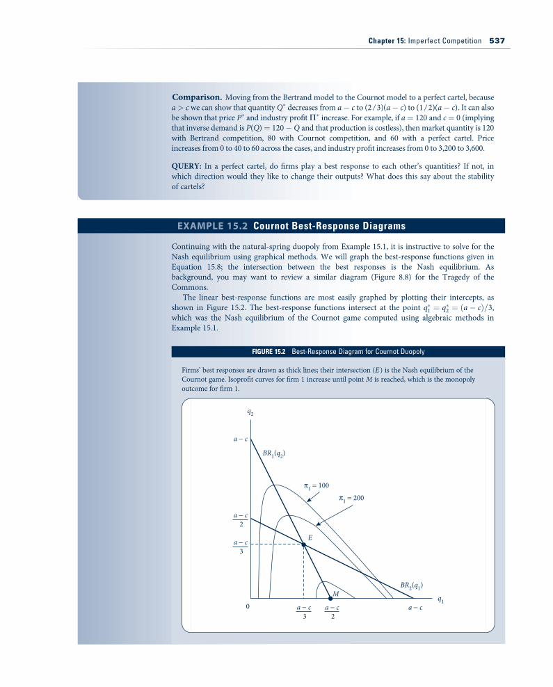
The linear best-response functions are most easily graphed by plotting their intercepts, asshown in Figure 15.2. The best-response functions intersect at the point q"1 ! q"2 ! (a$ c)=3,which was the Nash equilibrium of the Cournot game computed using algebraic methods inExample 15.1.

FIGURE 15.215Best-Response Diagram for Cournot Duopoly

Firms’ best responses are drawn as thick lines; their intersection (E ) is the Nash equilibrium of theCournot game. Isoprofit curves for firm 1 increase until point M is reached, which is the monopolyoutcome for firm 1.

a ! c

a ! c

a ! c

2

3

0

q2

q1M

E

BR1(q2)

BR2(q1)

"1 = 100

"1 = 200

a ! ca ! c2

a ! c3


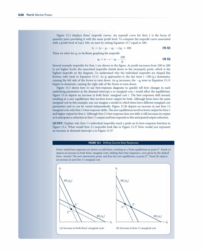
Figure 15.2 displays firms’ isoprofit curves. An isoprofit curve for firm 1 is the locus ofquantity pairs providing it with the same profit level. To compute the isoprofit curve associatedwith a profit level of (say) 100, we start by setting Equation 15.7 equal to 100:

p1 ! (a$ q1 $ q2 $ c)q1 ! 100: (15:12)

Then we solve for q2 to facilitate graphing the isoprofit:

q2 ! a$ c$ q1 $100q1

: (15:13)

Several example isoprofits for firm 1 are shown in the figure. As profit increases from 100 to 200to yet higher levels, the associated isoprofits shrink down to the monopoly point, which is thehighest isoprofit on the diagram. To understand why the individual isoprofits are shaped likefrowns, refer back to Equation 15.13. As ql approaches 0, the last term ($100 /q1) dominates,causing the left side of the frown to turn down. As ql increases, the $ql term in Equation 15.13begins to dominate, causing the right side of the frown to turn down.

Figure 15.3 shows how to use best-response diagrams to quickly tell how changes in suchunderlying parameters as the demand intercept a or marginal cost c would affect the equilibrium.Figure 15.3a depicts an increase in both firms’ marginal cost c. The best responses shift inward,resulting in a new equilibrium that involves lower output for both. Although firms have the samemarginal cost in this example, one can imagine a model in which firms have different marginal costparameters and so can be varied independently. Figure 15.3b depicts an increase in just firm 1’smarginal cost; only firm 1’s best response shifts. The new equilibrium involves lower output for firm 1and higher output for firm 2. Although firm 2’s best response does not shift, it still increases its outputas it anticipates a reduction in firm 1’s output and best responds to this anticipated output reduction.

QUERY: Explain why firm 1’s individual isoprofits reach a peak on its best-response function inFigure 15.2. What would firm 2’s isoprofits look like in Figure 15.2? How would you representan increase in demand intercept a in Figure 15.3?

FIGURE 15.315Shifting Cournot Best Responses

Firms’ initial best responses are drawn as solid lines, resulting in a Nash equilibrium at point E 0. Panel (a)depicts an increase in both firms’ marginal costs, shifting their best responses—now given by the dashedlines—inward. The new intersection point, and thus the new equilibrium, is point E 00. Panel (b) depictsan increase in just firm 1’s marginal cost.

q2 q2

BR1(q2) BR1(q2)

BR2(q1) BR2(q1)

q1 q1

E # E #

E$

E$

(a) Increase in both !rms’ marginal costs (b) Increase in !rm 1’s marginal cost


Varying the number of Cournot firmsThe Cournot model is particularly useful for policy analysis because it can represent thewhole range of outcomes from perfect competition to perfect cartel/monopoly (i.e., thewhole range of points between C and M in Figure 15.1) by varying the number of firmsn from n ! 1 to n ! 1. For simplicity, consider the case of identical firms, which heremeans the n firms sharing the same cost function C(qi). In equilibrium, firms will pro-duce the same share of total output: qi ! Q/n. Substituting qi ! Q/n into Equation 15.12,the wedge term becomes P 0(Q)Q/n. The wedge term disappears as n grows large; firmsbecome infinitesimally small. An infinitesimally small firm effectively becomes a price-taker because it produces so little that any decrease in market price from an increase inoutput hardly affects its revenue. Price approaches marginal cost and the market outcomeapproaches the perfectly competitive one. As n decreases to 1, the wedge term approachesthat in Equation 15.5, implying the Cournot outcome approaches that of a perfect cartel.As the Cournot firm’s market share grows, it internalizes the revenue loss from a decreasein market price to a greater extent.

EXAMPLE 15.3 Natural-Spring Oligopoly

Return to the natural springs in Example 15.1, but now consider a variable number n of firmsrather than just two. The profit of one of them, firm i, is

pi ! P(Q)qi $ cqi ! (a$ Q$ c)qi ! (a$ qi $ Q$i $ c)qi: (15:14)

It is convenient to express total output as Q ! qi ' Q$i, where Q$i ! Q $ qi is the output of allfirms except for i. Taking the first-order condition of Equation 15.14 with respect to qi, werecognize that firm i takes Q$i as a given and thus treats it as a constant in the differentiation,

@pi

@qi! a$ 2qi $ Q$i $ c ! 0, (15:15)

which holds for all i ! 1, 2, . . . , n.The key to solving the system of n equations for the n equilibrium quantities is to recognize

that the Nash equilibrium involves equal quantities because firms are symmetric. Symmetryimplies that

Q"$i ! Q" $ q"i ! nq"i $ q"i ! (n$ 1)q"i : (15:16)

Substituting Equation 15.16 into 15.15 yields

a$ 2q"i $ (n$ 1)q"i $ c ! 0, (15:17)

or q"i ! (a$ c)=(n' 1):Total market output is

Q" ! nq"i !n

n' 1

" #(a$ c), (15:18)

and market price is

P" ! a$ Q" ! 1n' 1

" #a' n

n' 1

" #c: (15:19)

Substituting for q"i , Q", and P" into the firm’s profit Equation 15.14, we have that total profit for

all firms is

P" ! np"i ! na$ cn' 1

" #2

: (15:20)


Prices or quantities?Moving from price competition in the Bertrand model to quantity competition in theCournot model changes the market outcome dramatically. This change is surprising onfirst thought. After all, the monopoly outcome from Chapter 14 is the same whether weassume the monopolist sets price or quantity. Further thought suggests why price andquantity are such different strategic variables. Starting from equal prices, a small reduc-tion in one firm’s price allows it to steal all the market demand from its competitors. Thissharp benefit from undercutting makes price competition extremely ‘‘tough.’’ Quantitycompetition is ‘‘softer.’’ Starting from equal quantities, a small increase in one firm’squantity has only a marginal effect on the revenue that other firms receive from theirexisting output. Firms have less of an incentive to outproduce each other with quantitycompetition than to undercut each other with price competition.

An advantage of the Cournot model is its realistic implication that the industry growsmore competitive as the number n of firms entering the market increases from monopolyto perfect competition. In the Bertrand model there is a discontinuous jump frommonopoly to perfect competition if just two firms enter, and additional entry beyond twohas no additional effect on the market outcome.

An apparent disadvantage of the Cournot model is that firms in real-world marketstend to set prices rather than quantities, contrary to the Cournot assumption that firmschoose quantities. For example, grocers advertise prices for orange juice, say, $3.00 a con-tainer, in newpaper circulars rather than the number of containers it stocks. As we willsee in the next section, the Cournot model applies even to the orange juice market if wereinterpret quantity to be the firm’s capacity, defined as the most the firm can sell giventhe capital it has in place and other available inputs in the short run.

Capacity ConstraintsFor the Bertrand model to generate the Bertrand paradox (the result that two firms essen-tially behave as perfect competitors), firms must have unlimited capacities. Starting fromequal prices, if a firm lowers its price the slightest amount, then its demand essentially dou-bles. The firm can satisfy this increased demand because it has no capacity constraints, giv-ing firms a big incentive to undercut. If the undercutting firm could not serve all thedemand at its lower price because of capacity constraints, that would leave some residualdemand for the higher-priced firm and would decrease the incentive to undercut.

Consider a two-stage game in which firms build capacity in the first stage and firmschoose prices p1 and p2 in the second stage.4 Firms cannot sell more in the second stage

Setting n ! 1 in Equations 15.18–15.20 gives the monopoly outcome, which gives the sameprice, total output, and profit as in the perfect cartel case computed in Example 15.1. Letting ngrow without bound in Equations 15.18–15.20 gives the perfectly competitive outcome, thesame outcome computed in Example 15.1 for the Bertrand case.

QUERY: We used the trick of imposing symmetry after taking the first-order condition for firm i’squantity choice. It might seem simpler to impose symmetry before taking the first-order condition.Why would this be a mistake? How would the incorrect expressions for quantity, price, and profitcompare with the correct ones here?

4The model is due to D. Kreps and J. Scheinkman, ‘‘Quantity Precommitment and Bertrand Competition Yield CournotOutcomes,’’ Bell Journal of Economics (Autumn 1983): 326–37.


than the capacity built in the first stage. If the cost of building capacity is sufficiently high,it turns out that the subgame-perfect equilibrium of this sequential game leads to thesame outcome as the Nash equilibrium of the Cournot model.

To see this result, we will analyze the game using backward induction. Consider thesecond-stage pricing game supposing the firms have already built capacities q1 and q2 inthe first stage. Let p be the price that would prevail when production is at capacity forboth firms. A situation in which

p1 ! p2 < p (15:21)

is not a Nash equilibrium. At this price, total quantity demanded exceeds total capacity;therefore, firm 1 could increase its profits by raising price slightly and continuing to sell q1.Similarly,

p1 ! p2 > p (15:22)

is not a Nash equilibrium because now total sales fall short of capacity. At least one firm(say, firm 1) is selling less than its capacity. By cutting price slightly, firm 1 can increaseits profits by selling up to its capacity, q1. Hence the Nash equilibrium of this second-stage game is for firms to choose the price at which quantity demanded exactly equals thetotal capacity built in the first stage:5

p1 ! p2 ! p: (15:23)

Anticipating that the price will be set such that firms sell all their capacity, the first-stage capacity choice game is essentially the same as the Cournot game. Therefore, theequilibrium quantities, price, and profits will be the same as in the Cournot game. Thus,even in markets (such as orange juice sold in grocery stores) where it looks like firms aresetting prices, the Cournot model may prove more realistic than it first seems.

Product DifferentiationAnother way to avoid the Bertrand paradox is to replace the assumption that the firms’products are identical with the assumption that firms produce differentiated products.Many (if not most) real-world markets exhibit product differentiation. For example,toothpaste brands vary somewhat from supplier to supplier—differing in flavor, fluoridecontent, whitening agents, endorsement from the American Dental Association, and soforth. Even if suppliers’ product attributes are similar, suppliers may still be differentiatedin another dimension: physical location. Because demanders will be closer to some sup-pliers than to others, they may prefer nearby sellers because buying from them involvesless travel time.

Meaning of ‘‘the market’’The possibility of product differentiation introduces some fuzziness into what we meanby the market for a good. With identical products, demanders were assumed to be indif-ferent about which firm’s output they bought; hence they shop at the lowest-price firm,leading to the law of one price. The law of one price no longer holds if demanders strictly

5For completeness, it should be noted that there is no pure-strategy Nash equilibrium of the second-stage game with unequalprices (p1 6! p2). The low-price firm would have an incentive to increase its price and/or the high-price firm would have an in-centive to lower its price. For large capacities, there may be a complicated mixed-strategy Nash equilibrium, but this can beruled out by supposing the cost of building capacity is sufficiently high.


prefer one supplier to another at equal prices. Are green-gel and white-paste toothpastesin the same market or in two different ones? Is a pizza parlor at the outskirts of town inthe same market as one in the middle of town?

With differentiated products, we will take the market to be a group of closely relatedproducts that are more substitutable among each other (as measured by cross-price elas-ticities) than with goods outside the group. We will be somewhat loose with this defini-tion, avoiding precise thresholds for how high the cross-price elasticity must be betweengoods within the group (and how low with outside goods). Arguments about which goodsshould be included in a product group often dominate antitrust proceedings, and we willtry to avoid this contention here.

Bertrand competition with differentiated productsReturn to the Bertrand model but now suppose there are n firms that simultaneouslychoose prices pi (i ! 1, . . . , n) for their differentiated products. Product i has its ownspecific attributes ai, possibly reflecting special options, quality, brand advertising, orlocation. A product may be endowed with the attribute (orange juice is by definitionmade from oranges and cranberry juice from cranberries), or the attribute may be theresult of the firm’s choice and spending level (the orange juice supplier can spend moreand make its juice from fresh oranges rather than from frozen concentrate). The variousattributes serve to differentiate the products. Firm i’s demand is

qi( pi, P$i, ai, A$i), (15:24)

where P$i is a list of all other firms’ prices besides i’s, and A$i is a list of all other firms’attributes besides i’s. Firm i’s total cost is

Ci(qi, ai) (15:25)

and profit is thus

pi ! piqi $ Ci(qi, ai): (15:26)

With differentiated products, the profit function (Equation 15.26) is differentiable, sowe do not need to solve for the Nash equilibrium on a case-by-case basis as we did in theBertrand model with identical products. We can solve for the Nash equilibrium as in theCournot model, solving for best-response functions by taking each firm’s first-order con-dition (here with respect to price rather than quantity). The first-order condition fromEquation 15.26 with respect to pi is

@pi

@pi! qi ' pi

@qi@pi|!!!!!!{z!!!!!!}

A

$ @Ci

@qi& @qi@pi|!!!!{z!!!!}

B

! 0: (15:27)

The first two terms (labeled A) on the right side of Equation 15.27 are a sort of marginalrevenue—not the usual marginal revenue from an increase in quantity, but rather themarginal revenue from an increase in price. The increase in price increases revenue onexisting sales of qi units, but we must also consider the negative effect of the reduction insales (@qi/@pi multiplied by the price pi) that would have been earned on these sales. Thelast term, labeled B, is the cost savings associated with the reduced sales that accompanyan increased price.

The Nash equilibrium can be found by simultaneously solving the system of first-orderconditions in Equation 15.27 for all i ! 1, . . . , n. If the attributes ai are also choice


variables (rather than just endowments), there will be another set of first-order conditionsto consider. For firm i, the first-order condition with respect to ai has the form

@pi

@ai! pi

@qi@ai$ @Ci

@ai$ @Ci

@qi& @qi@ai! 0: (15:28)

The simultaneous solution of these first-order conditions can be complex, and they yieldfew definitive conclusions about the nature of market equilibrium. Some insights fromparticular cases will be developed in the next two examples.

EXAMPLE 15.4 Toothpaste as a Differentiated Product

Suppose that two firms produce toothpaste, one a green gel and the other a white paste. Tosimplify the calculations, suppose that production is costless. Demand for product i is

qi ! ai $ pi 'pj2: (15:29)

The positive coefficient on pj, the other good’s price, indicates that the goods are gross substitutes.Firm i’s demand is increasing in the attribute ai, which we will take to be demanders’ inherentpreference for the variety in question; we will suppose that this is an endowment rather than achoice variable for the firm (and so will abstract from the role of advertising to promotepreferences for a variety).

Algebraic solution. Firm i’s profit is

pi ! piqi $ Ci(qi) ! pi ai $ pi 'pj2

$ %, (15:30)

where Ci(qi) ! 0 because i’s production is costless. The first-order condition for profit maximizationwith respect to pi is

@pi

@pi! ai $ 2pi '

pj2! 0: (15:31)

Solving for pi gives the following best-response functions for i ! 1, 2:

p1 !12

a1 'p22

$ %, p2 !

12

a2 'p12

$ %: (15:32)

Solving Equations 15.32 simultaneously gives the Nash equilibrium prices

p"i !815

ai '215

aj: (15:33)

The associated profits are

p"i !815

ai '215

aj

" #2

: (15:34)

Firm i’s equilibrium price is not only increasing in its own attribute, ai, but also in the otherproduct’s attribute, aj. An increase in aj causes firm j to increase its price, which increases firmi’s demand and thus the price i charges.

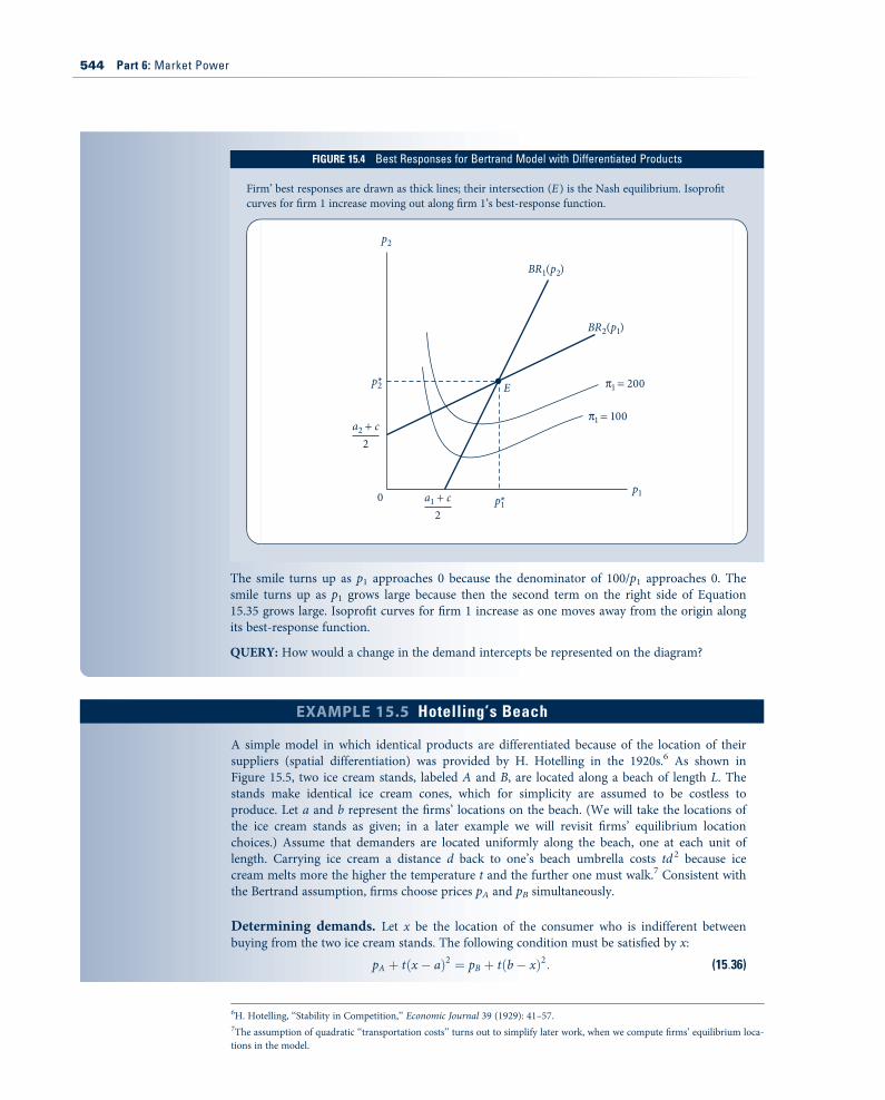
Graphical solution. We could also have solved for equilibrium prices graphically, as in Figure 15.4.The best responses in Equation 15.32 are upward sloping. They intersect at the Nash equilibrium,point E. The isoprofit curves for firm 1 are smile-shaped. To see this, take the expression for firm 1’sprofit in Equation 15.30, set it equal to a certain profit level (say, 100), and solve for p2 to facilitategraphing it on the best-response diagram.Wehave

p2 !100p1' p1 $ a1: (15:35)


EXAMPLE 15.5 Hotelling’s Beach

A simple model in which identical products are differentiated because of the location of theirsuppliers (spatial differentiation) was provided by H. Hotelling in the 1920s.6 As shown inFigure 15.5, two ice cream stands, labeled A and B, are located along a beach of length L. Thestands make identical ice cream cones, which for simplicity are assumed to be costless toproduce. Let a and b represent the firms’ locations on the beach. (We will take the locations ofthe ice cream stands as given; in a later example we will revisit firms’ equilibrium locationchoices.) Assume that demanders are located uniformly along the beach, one at each unit oflength. Carrying ice cream a distance d back to one’s beach umbrella costs td 2 because icecream melts more the higher the temperature t and the further one must walk.7 Consistent withthe Bertrand assumption, firms choose prices pA and pB simultaneously.

Determining demands. Let x be the location of the consumer who is indifferent betweenbuying from the two ice cream stands. The following condition must be satisfied by x:

pA ' t(x $ a)2 ! pB ' t(b$ x)2: (15:36)

The smile turns up as p1 approaches 0 because the denominator of 100/p1 approaches 0. Thesmile turns up as p1 grows large because then the second term on the right side of Equation15.35 grows large. Isoprofit curves for firm 1 increase as one moves away from the origin alongits best-response function.

QUERY: How would a change in the demand intercepts be represented on the diagram?

FIGURE 15.415Best Responses for Bertrand Model with Differentiated Products

Firm’ best responses are drawn as thick lines; their intersection (E ) is the Nash equilibrium. Isoprofitcurves for firm 1 increase moving out along firm 1’s best-response function.

p2

p1

E

p1*

p2*

a2 + c2

0 a1 + c2

BR1(p2)

BR2(p1)

"1 = 100

"1 = 200

6H. Hotelling, ‘‘Stability in Competition,’’ Economic Journal 39 (1929): 41–57.7The assumption of quadratic ‘‘transportation costs’’ turns out to simplify later work, when we compute firms’ equilibrium loca-tions in the model.


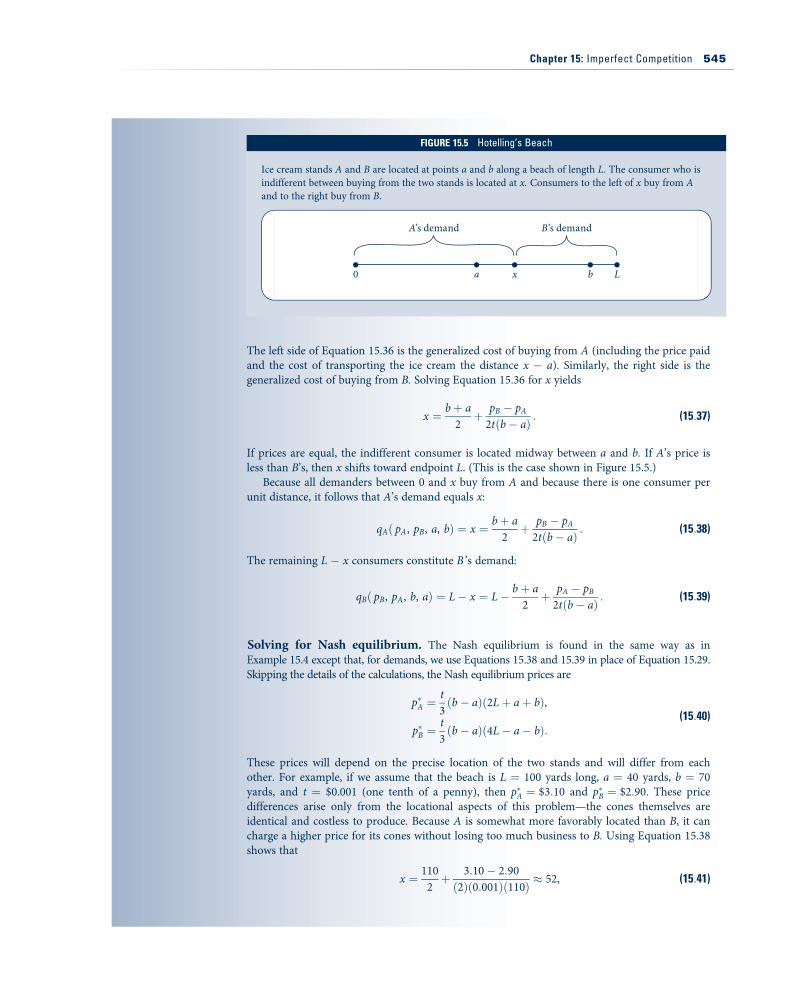
The left side of Equation 15.36 is the generalized cost of buying from A (including the price paidand the cost of transporting the ice cream the distance x $ a). Similarly, the right side is thegeneralized cost of buying from B. Solving Equation 15.36 for x yields

x ! b' a2' pB $ pA2t(b$ a)

: (15:37)

If prices are equal, the indifferent consumer is located midway between a and b. If A’s price isless than B’s, then x shifts toward endpoint L. (This is the case shown in Figure 15.5.)

Because all demanders between 0 and x buy from A and because there is one consumer perunit distance, it follows that A’s demand equals x:

qA( pA, pB, a, b) ! x ! b' a2' pB $ pA2t(b$ a)

: (15:38)

The remaining L $ x consumers constitute B ’s demand:

qB( pB, pA, b, a) ! L$ x ! L$ b' a2' pA $ pB2t(b$ a)

: (15:39)

Solving for Nash equilibrium. The Nash equilibrium is found in the same way as inExample 15.4 except that, for demands, we use Equations 15.38 and 15.39 in place of Equation 15.29.Skipping the details of the calculations, the Nash equilibrium prices are

p"A !t3(b$ a)(2L' a' b),

p"B !t3(b$ a)(4L$ a$ b):

(15:40)

These prices will depend on the precise location of the two stands and will differ from eachother. For example, if we assume that the beach is L ! 100 yards long, a ! 40 yards, b ! 70yards, and t ! $0.001 (one tenth of a penny), then p"A ! $3:10 and p"B ! $2:90. These pricedifferences arise only from the locational aspects of this problem—the cones themselves areidentical and costless to produce. Because A is somewhat more favorably located than B, it cancharge a higher price for its cones without losing too much business to B. Using Equation 15.38shows that

x ! 1102' 3:10$ 2:90(2)(0:001)(110)

* 52, (15:41)

FIGURE 15.515Hotelling’s Beach

Ice cream stands A and B are located at points a and b along a beach of length L. The consumer who isindifferent between buying from the two stands is located at x. Consumers to the left of x buy from Aand to the right buy from B.

A’s demand B’s demand

a0 x b L


Consumer search and price dispersionHotelling’s model analyzed in Example 15.5 suggests the possibility that competitors mayhave some ability to charge prices above marginal cost and earn positive profits even ifthe physical characteristics of the goods they sell are identical. Firms’ various locations—closer to some demanders and farther from others—may lead to spatial differentiation.The Internet makes the physical location of stores less relevant to consumers, especially ifshipping charges are independent of distance (or are not assessed). Even in this setting,firms can avoid the Bertrand paradox if we drop the assumption that demanders knowevery firm’s price in the market. Instead we will assume that demanders face a small costs, called a search cost, to visit the store (or click to its website) to find its price.

Peter Diamond, winner of the Nobel Prize in economics in 2010, developed a modelin which demanders search by picking one of the n stores at random and learning itsprice. Demanders know the equilibrium distribution of prices but not which store ischarging which price. Demanders get their first price search for free but then must pay sfor additional searches. They need at most one unit of the good, and they all have thesame gross surplus v for the one unit.8

Not only do stores manage to avoid the Bertrand paradox in this model, they obtainthe polar opposite outcome: All charge the monopoly price v, which extracts all consumersurplus! This outcome holds no matter how small the search cost s is—as long as s is pos-itive (say, a penny). It is easy to see that all stores charging v is an equilibrium. If allcharge the same price v, then demanders may as well buy from the first store they searchbecause additional searches are costly and do not end up revealing a lower price. It canalso be seen that this is the only equilibrium. Consider any outcome in which at least onestore charges less than v, and consider the lowest-price store (label it i) in this outcome.

so stand A sells 52 cones, whereas B sells only 48 despite its lower price. At point x, theconsumer is indifferent between walking the 12 yards to A and paying $3.10 or walking 18 yardsto B and paying $2.90. The equilibrium is inefficient in that a consumer slightly to the right of xwould incur a shorter walk by patronizing A but still chooses B because of A’s power to sethigher prices.

Equilibrium profits are

p"A !t18(b$ a)(2L' a' b)2,

p"B !t18(b$ a)(4L$ a$ b)2:

(15:42)

Somewhat surprisingly, the ice cream stands benefit from faster melting, as measured here bythe transportation cost t. For example, if we take L ! 100, a ! 40, b ! 70, and t ! $0.001 as inthe previous paragraph, then p"A ! $160 and p"B ! $140 (rounding to the nearest dollar). Iftransportation costs doubled to t ! $0.002, then profits would double to p"A ! $320 andp"B ! $280.

The transportation/melting cost is the only source of differentiation in the model. If t ! 0,then we can see from Equation 15.40 that prices equal 0 (which is marginal cost given thatproduction is costless) and from Equation 15.42 that profits equal 0—in other words, theBertrand paradox results.

QUERY: What happens to prices and profits if ice cream stands locate in the same spot? If theylocate at the opposite ends of the beach?

8P. Diamond, ‘‘A Model of Price Adjustment,’’ Journal of Economic Theory 3 (1971): 156–68.


Store i could raise its price pi by as much as s and still make all the sales it did before.The lowest price a demander could expect to pay elsewhere is no less than pt, and thedemander would have to pay the cost s to find this other price.

Less extreme equilibria are found in models where consumers have different searchcosts.9 For example, suppose one group of consumers can search for free and anothergroup has to pay s per search. In equilibrium, there will be some price dispersion acrossstores. One set of stores serves the low–search-cost demanders (and the lucky high–search-cost consumers who happen to stumble on a bargain). These bargain stores sell atmarginal cost. The other stores serve the high–search-cost demanders at a price thatmakes these demanders indifferent between buying immediately and taking a chance thatthe next price search will uncover a bargain store.

Tacit CollusionIn Chapter 8, we showed that players may be able to earn higher payoffs in the subgame-perfect equilibrium of an infinitely repeated game than from simply repeating the Nashequilibrium from the single-period game indefinitely. For example, we saw that, if playersare patient enough, they can cooperate on playing silent in the infinitely repeated versionof the Prisoners’ Dilemma rather than finking on each other each period. From the per-spective of oligopoly theory, the issue is whether firms must endure the Bertrand paradox(marginal cost pricing and zero profits) in each period of a repeated game or whetherthey might instead achieve more profitable outcomes through tacit collusion.

A distinction should be drawn between tacit collusion and the formation of an explicitcartel. An explicit cartel involves legal agreements enforced with external sanctions if theagreements (e.g., to sustain high prices or low outputs) are violated. Tacit collusion canonly be enforced through punishments internal to the market—that is, only those thatcan be generated within a subgame-perfect equilibrium of a repeated game. Antitrust lawsgenerally forbid the formation of explicit cartels, so tacit collusion is usually the only wayfor firms to raise prices above the static level.

Finitely repeated gameTaking the Bertrand game to be the stage game, Selten’s theorem from Chapter 8 tells usthat repeating the stage game any finite number of times T does not change the outcome.The only subgame-perfect equilibrium of the finitely repeated Bertrand game is to repeatthe stage-game Nash equilibrium—marginal cost pricing—in each of the T periods. Thegame unravels through backward induction. In any subgame starting in period T, theunique Nash equilibrium will be played regardless of what happened before. Becausethe outcome in period T $ 1 does not affect the outcome in the next period, it is asthough period T $ 1 is the last period, and the unique Nash equilibrium must be playedthen, too. Applying backward induction, the game unravels in this manner all the wayback to the first period.

Infinitely repeated gameIf the stage game is repeated infinitely many periods, however, the folk theorem applies.The folk theorem indicates that any feasible and individually rational payoff can be sus-tained each period in an infinitely repeated game as long as the discount factor, d, is closeenough to unity. Recall that the discount factor is the value in the present period of one

9The following model is due to S. Salop and J. Stiglitz, ‘‘Bargains and Ripoffs: A Model of Monopolistically Competitive PriceDispersion,’’ Review of Economic Studies 44 (1977): 493–510.


dollar earned one period in the future—a measure, roughly speaking, of how patient play-ers are. Because the monopoly outcome (with profits divided among the firms) is a feasi-ble and individually rational outcome, the folk theorem implies that the monopolyoutcome must be sustainable in a subgame-perfect equilibrium for d close enough to 1.Let’s investigate the threshold value of d needed.

First suppose there are two firms competing in a Bertrand game each period. Let GM

denote the monopoly profit and PM the monopoly price in the stage game. The firmsmay collude tacitly to sustain the monopoly price—with each firm earning an equal shareof the monopoly profit—by using the grim trigger strategy of continuing to collude aslong as no firm has undercut PM in the past but reverting to the stage-game Nash equilib-rium of marginal cost pricing every period from then on if any firm deviates by undercut-ting. Successful tacit collusion provides the profit stream

Vcollude ! PM

2' d &PM

2' d2 &PM

2' & & &

! PM

2(1' d' d2 ' & & &)

! PM

2

" #1

1$ d

" #: (15:43)

Refer to Chapter 8 for a discussion of adding up a series of discount factors1' d' d2 ' & & &. We need to check that a firm has no incentive to deviate. By undercut-ting the collusive price PM slightly, a firm can obtain essentially all the monopoly profitfor itself in the current period. This deviation would trigger the grim strategy punishmentof marginal cost pricing in the second and all future periods, so all firms would earn zeroprofit from there on. Hence the stream of profits from deviating is V deviate ! GM.

For this deviation not to be profitable wemust haveV collude%V deviate or, on substituting,

PM

2

" #1

1$ d

" #% PM: (15:44)

Rearranging Equation 15.44, the condition reduces to d % 1/2. To prevent deviation,firms must value the future enough that the threat of losing profits by reverting to theone-period Nash equilibrium outweighs the benefit of undercutting and taking the wholemonopoly profit in the present period.

EXAMPLE 15.6 Tacit Collusion in a Bertrand Model

Bertrand duopoly. Suppose only two firms produce a certain medical device used in surgery.The medical device is produced at constant average and marginal cost of $10, and the demandfor the device is given by

Q ! 5,000$ 100P: (15:45)

If the Bertrand game is played in a single period, then each firm will charge $10 and a total of4,000 devices will be sold. Because the monopoly price in this market is $30, firms have a clearincentive to consider collusive strategies. At the monopoly price, total profits each period are$40,000, and each firm’s share of total profits is $20,000. According to Equation 15.44, collusionat the monopoly price is sustainable if

20,0001

1$ d

" #% 40,000 (15:46)

or if d % 1/2, as we saw.


Is the condition d % 1/2 likely to be met in this market? That depends on what factors weconsider in computing d, including the interest rate and possible uncertainty about whether thegame will continue. Leave aside uncertainty for a moment and consider only the interest rate. Ifthe period length is one year, then it might be reasonable to assume an annual interest rate ofr ! 10%. As shown in the Appendix to Chapter 17, d ! 1/(1 ' r); therefore, if r ! 10%, thend ! 0.91. This value of d clearly exceeds the threshold of 1/2 needed to sustain collusion. For dto be less than the 1/2 threshold for collusion, we must incorporate uncertainty into thediscount factor. There must be a significant chance that the market will not continue into thenext period—perhaps because a new surgical procedure is developed that renders the medicaldevice obsolete.

We focused on the best possible collusive outcome: the monopoly price of $30. Wouldcollusion be easier to sustain at a lower price, say $20? No. At a price of $20, total profits eachperiod are $30,000, and each firm’s share is $15,000. Substituting into Equation 15.44, collusioncan be sustained if

15,0001

1$ d

" #% 30,000, (15:47)

again implying d % 1/2. Whatever collusive profit the firms try to sustain will cancel out fromboth sides of Equation 15.44, leaving the condition d % 1/2. Therefore, we get a discrete jump infirms’ ability to collude as they become more patient—that is, as d increases from 0 to 1.10 For dbelow 1/2, no collusion is possible. For d above 1/2, any price between marginal cost and themonopoly price can be sustained as a collusive outcome. In the face of this multiplicity ofsubgame-perfect equilibria, economists often focus on the one that is most profitable for thefirms, but the formal theory as to why firms would play one or another of the equilibria is stillunsettled.

Bertrand oligopoly. Now suppose n firms produce the medical device. The monopoly profitcontinues to be $40,000, but each firm’s share is now only $40,000/n. By undercutting themonopoly price slightly, a firm can still obtain the whole monopoly profit for itself regardless ofhow many other firms there are. Replacing the collusive profit of $20,000 in Equation 15.46 with$40,000/n, we have that the n firms can successfully collude on the monopoly price if

40,000n

11$ d

" #% 40,000, (15:48)

or

d % 1$ 1n: (15:49)

Taking the ‘‘reasonable’’ discount factor of d ! 0.91 used previously, collusion is possible when11 or fewer firms are in the market and impossible with 12 or more. With 12 or more firms, theonly subgame-perfect equilibrium involves marginal cost pricing and zero profits.

Equation 15.49 shows that tacit collusion is easier the more patient are firms (as we sawbefore) and the fewer of them there are. One rationale used by antitrust authorities to challengecertain mergers is that a merger may reduce n to a level such that Equation 15.49 begins to besatisfied and collusion becomes possible, resulting in higher prices and lower total welfare.

QUERY: A period can be interpreted as the length of time it takes for firms to recognizeand respond to undercutting by a rival. What would be the relevant period for competinggasoline stations in a small town? In what industries would a year be a reasonable period?

10The discrete jump in firms’ ability to collude is a feature of the Bertrand model; the ability to collude increases continuouslywith d in the Cournot model of Example 15.7.


EXAMPLE 15.7 Tacit Collusion in a Cournot Model

Suppose that there are again two firms producing medical devices but that each period they nowengage in quantity (Cournot) rather than price (Bertrand) competition. We will again investigatethe conditions under which firms can collude on the monopoly outcome. To generate themonopoly outcome in a period, firms need to produce 1,000 each; this leads to a price of $30,total profits of $40,000, and firm profits of $20,000. The present discounted value of the stream ofthese collusive profits is

V collude ! 20,0001

1$ d

" #: (15:50)

Computing the present discounted value of the stream of profits from deviating is somewhatcomplicated. The optimal deviation is not as simple as producing the whole monopoly outputoneself and having the other firm produce nothing. The other firm’s 1,000 units would beprovided to the market. The optimal deviation (by firm 1, say) would be to best respond to firm2’s output of 1,000. To compute this best response, first note that if demand is given byEquation 15.45, then inverse demand is given by

P ! 50$ Q100

: (15:51)

Firm 1’s profit is

p1 ! Pq1 $ cq1 ! q1 40$ q1 ' q2100

$ %: (15:52)

Taking the first-order condition with respect to q1 and solving for q1 yields the best-responsefunction

q1 ! 2,000$ q22: (15:53)

Firm 1’s optimal deviation when firm 2 produces 1,000 units is to increase its output from 1,000to 1,500. Substituting these quantities into Equation 15.52 implies that firm 1 earns $22,500 inthe period in which it deviates.

How much firm 1 earns in the second and later periods following a deviation depends on thetrigger strategies firms use to punish deviation. Assume that firms use the grim strategy ofreverting to the Nash equilibrium of the stage game—in this case, the Nash equilibrium of theCournot game—every period from then on. In the Nash equilibrium of the Cournot game, eachfirm best responds to the other in accordance with the best-response function in Equation 15.53(switching subscripts in the case of firm 2). Solving these best-response equations simultaneouslyimplies that the Nash equilibrium outputs are q"1 ! q"2 ! 4,000=3 and that profits arep"1 ! p"2 ! $17,778. Firm 1’s present discounted value of the stream of profits from deviation is

V deviate ! 22,500' 17,778 & d' 17,778 & d2 ' 17,778 & d3 ' & & &! 22,500' (17,778 & d)(1' d' d2 ' & & &)

! $22,500' $17,778d

1$ d

" #: (15:54)

We have V collude % V deviate if

$20,0001

1$ d

" #% $22,500' $17,778

d1$ d

" #(15:55)

or, after some algebra, if d % 0.53.Unlike with the Bertrand stage game, with the Cournot stage game there is a possibility of

some collusion for discount factors below 0.53. However, the outcome would have to involvehigher outputs and lower profits than monopoly.


Longer-Run Decisions: Investment,Entry, And ExitThe chapter has so far focused on the most basic short-run decisions regarding whatprice or quantity to set. The scope for strategic interaction expands when we introducelonger-run decisions. Take the case of the market for cars. Longer-run decisions includewhether to update the basic design of the car, a process that might take up to two yearsto complete. Longer-run decisions may also include investing in robotics to lower pro-duction costs, moving manufacturing plants closer to consumers and cheap inputs,engaging in a new advertising campaign, and entering or exiting certain product lines(say, ceasing the production of station wagons or starting production of hybrid cars). Inmaking such decisions, an oligopolist must consider how rivals will respond to it. Willcompetition with existing rivals become tougher or milder? Will the decision lead to theexit of current rivals or encourage new ones to enter? Is it better to be the first to makesuch a decision or to wait until after rivals move?

Flexibility versus commitmentCrucial to our analysis of longer-run decisions such as investment, entry, and exit is how easyit is to reverse a decision once it has been made. On first thought, it might seem that it is bet-ter for a firm to be able to easily reverse decisions because this would give the firm more flexi-bility in responding to changing circumstances. For example, a car manufacturer might bemore willing to invest in developing a hybrid-electric car if it could easily change the designback to a standard gasoline-powered one should the price of gasoline (and the demand forhybrid cars along with it) decrease unexpectedly. Absent strategic considerations—and so forthe case of a monopolist—a firm would always value flexibility and reversibility. The ‘‘optionvalue’’ provided by flexibility is discussed in further detail in Chapter 7.

Surprisingly, the strategic considerations that arise in an oligopoly setting may lead afirm to prefer its decision be irreversible. What the firm loses in terms of flexibility maybe offset by the value of being able to commit to the decision. We will see a number ofinstances of the value of commitment in the next several sections. If a firm can committo an action before others move, the firm may gain a first-mover advantage. A firm mayuse its first-mover advantage to stake out a claim to a market by making a commitmentto serve it and in the process limit the kinds of actions its rivals find profitable. Commit-ment is essential for a first-mover advantage. If the first mover could secretly reverse itsdecision, then its rival would anticipate the reversal and the firms would be back in thegame with no first-mover advantage.

We already encountered a simple example of the value of commitment in the Battle ofthe Sexes game from Chapter 8. In the simultaneous version of the model, there werethree Nash equilibria. In one pure-strategy equilibrium, the wife obtains her highest pay-off by attending her favorite event with her husband, but she obtains lower payoffs in theother two equilibria (a pure-strategy equilibrium in which she attends her less favored

QUERY: The benefit to deviating is lower with the Cournot stage game than with the Bertrandstage game because the Cournot firm cannot steal all the monopoly profit with a smalldeviation. Why then is a more stringent condition (d % 0.53 rather than d % 0.5) needed tocollude on the monopoly outcome in the Cournot duopoly compared with the Bertrandduopoly?


event and a mixed-strategy equilibrium giving her the lowest payoff of all three). In thesequential version of the game, if a player were given the choice between being the firstmover and having the ability to commit to attending an event or being the second moverand having the flexibility to be able to meet up with the first wherever he or she showedup, a player would always choose the ability to commit. The first mover can guaranteehis or her preferred outcome as the unique subgame-perfect equilibrium by committingto attend his or her favorite event.

Sunk costsExpenditures on irreversible investments are called sunk costs.

Sunk costs include expenditures on unique types of equipment (e.g., a newsprint-makingmachine) or job-specific training for workers (developing the skills to use the newsprintmachine). There is sometimes confusion between sunk costs and what we have calledfixed costs. They are similar in that they do not vary with the firm’s output level in a pro-duction period and are incurred even if no output is produced in that period. But insteadof being incurred periodically, as are many fixed costs (heat for the factory, salaries forsecretaries and other administrators), sunk costs are incurred only once in connectionwith a single investment.11 Some fixed costs may be avoided over a sufficiently longrun—say, by reselling the plant and equipment involved—but sunk costs can never berecovered because the investments involved cannot be moved to a different use. Whenthe firm makes a sunk investment, it has committed itself to that investment, and thismay have important consequences for its strategic behavior.

First-mover advantage in the Stackelberg modelThe simplest setting to illustrate the first-mover advantage is in the Stackelberg model,named after the economist who first analyzed it.12 The model is similar to a duopoly ver-sion of the Cournot model except that—rather than simultaneously choosing the quanti-ties of their identical outputs—firms move sequentially, with firm 1 (the leader) choosingits output first and then firm 2 (the follower) choosing after observing firm 1’s output.

We use backward induction to solve for the subgame-perfect equilibrium of this se-quential game. Begin with the follower’s output choice. Firm 2 chooses the output q2 thatmaximizes its own profit, taking firm 1’s output as given. In other words, firm 2 bestresponds to firm 1’s output. This results in the same best-response function for firm 2 aswe computed in the Cournot game from the first-order condition (Equation 15.2). Labelthis best-response function BR2(q1).

Turn then to the leader’s output choice. Firm 1 recognizes that it can influence the fol-lower’s action because the follower best responds to 1’s observed output. SubstitutingBR2(q1) into the profit function for firm 1 given by Equation 15.1, we have

p1 ! P (q1 ' BR2(q1))q1 $ C1(q1): (15:56)

D E F I N I T I O N Sunk cost. A sunk cost is an expenditure on an investment that cannot be reversed and has noresale value.

11Mathematically, the notion of sunk costs can be integrated into the per-period total cost function as

Ct (qt) ! S ' Ft ' cqt,

where S is the per-period amortization of sunk costs (e.g., the interest paid for funds used to finance capital investments), Ft isthe per-period fixed costs, c is marginal cost, and qt is per-period output. If qt ! 0, then Ct ! S ' Ft; but if the productionperiod is long enough, then some or all of Ft may also be avoidable. No portion of S is avoidable, however.12H. von Stackelberg, The Theory of the Market Economy, trans. A. T. Peacock (New York: Oxford University Press, 1952).


The first-order condition with respect to q1 is

@p1

@q1! P(Q) ' P 0(Q)q1 ' P 0(Q)BR2

0(q1)q1|!!!!!!!!!!!!{z!!!!!!!!!!!!}S

$Ci0(qi) ! 0: (15:57)

This is the same first-order condition computed in the Cournot model (see Equation15.2) except for the addition of the term S, which accounts for the strategic effect of firm1’s output on firm 2’s. The strategic effect S will lead firm 1 to produce more than itwould have in a Cournot model. By overproducing, firm 1 leads firm 2 to reduce q2 bythe amount BR02(q1); the fall in firm 2’s output increases market price, thus increasing therevenue that firm 1 earns on its existing sales. We know that q2 decreases with an increasein ql because best-response functions under quantity competition are generally downwardsloping; see Figure 15.2 for an illustration.

The strategic effect would be absent if the leader’s output choice were unobservable tothe follower or if the leader could reverse its output choice in secret. The leader must beable to commit to an observable output choice or else firms are back in the Cournotgame. It is easy to see that the leader prefers the Stackelberg game to the Cournot game.The leader could always reproduce the outcome from the Cournot game by choosing itsCournot output in the Stackelberg game. The leader can do even better by producingmore than its Cournot output, thereby taking advantage of the strategic effect S.

EXAMPLE 15.8 Stackelberg Springs

Recall the two natural-spring owners from Example 15.1. Now, rather than having them chooseoutputs simultaneously as in the Cournot game, assume that they choose outputs sequentially asin the Stackelberg game, with firm 1 being the leader and firm 2 the follower.

Firm 2’s output. We will solve for the subgame-perfect equilibrium using backward induction,starting with firm 2’s output choice. We already found firm 2’s best-response function inEquation 15.8, repeated here:

q2 !a$ q1 $ c

2: (15:58)

Firm 1’s output. Now fold the game back to solve for firm 1’s output choice. Substituting firm2’s best response from Equation 15.58 into firm 1’s profit function from Equation 15.56 yields

p1 ! a$ q1 $a$ q1 $ c

2

$ %$ c

h iq1 !

12(a$ q1 $ c)q1: (15:59)

Taking the first-order condition,

@p1

@q1! 1

2(a$ 2q1 $ c) ! 0, (15:60)

and solving gives q"1 ! (a$ c)=2. Substituting q"1 back into firm 2’s best-response function givesq"2 ! (a$ c)=4. Profits are p"1 ! (1=8)(a$ c)2 and p"2 ! (1=16)(a$ c)2.

To provide a numerical example, suppose a ! 120 and c ! 0. Then q"1 ! 60, q"2 ! 30,p"1 ! $1,800, and p"2 ! $900. Firm 1 produces twice as much and earns twice as much as firm 2.Recall from the simultaneous Cournot game in Example 15.1 that, for these numerical values,total market output was 80 and total industry profit was 3,200, implying that each of the twofirms produced 80/2 ! 40 units and earned $3,200/2 ! $1,600. Therefore, when firm 1 is the


first mover in a sequential game, it produces (60 $ 40)/40 ! 50% more and earns (1,800 $1,600)/1,600 ! 12.5% more than in the simultaneous game.

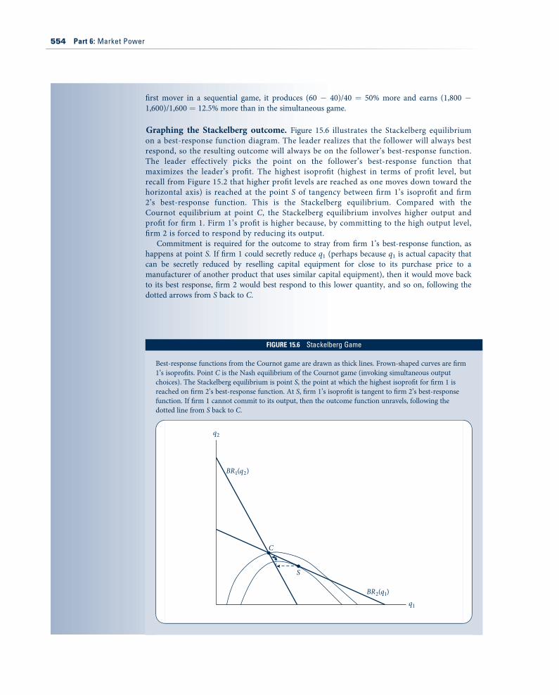
Graphing the Stackelberg outcome. Figure 15.6 illustrates the Stackelberg equilibriumon a best-response function diagram. The leader realizes that the follower will always bestrespond, so the resulting outcome will always be on the follower’s best-response function.The leader effectively picks the point on the follower’s best-response function thatmaximizes the leader’s profit. The highest isoprofit (highest in terms of profit level, butrecall from Figure 15.2 that higher profit levels are reached as one moves down toward thehorizontal axis) is reached at the point S of tangency between firm 1’s isoprofit and firm2’s best-response function. This is the Stackelberg equilibrium. Compared with theCournot equilibrium at point C, the Stackelberg equilibrium involves higher output andprofit for firm 1. Firm 1’s profit is higher because, by committing to the high output level,firm 2 is forced to respond by reducing its output.

Commitment is required for the outcome to stray from firm 1’s best-response function, ashappens at point S. If firm 1 could secretly reduce q1 (perhaps because q1 is actual capacity thatcan be secretly reduced by reselling capital equipment for close to its purchase price to amanufacturer of another product that uses similar capital equipment), then it would move backto its best response, firm 2 would best respond to this lower quantity, and so on, following thedotted arrows from S back to C.

FIGURE 15.615Stackelberg Game

Best-response functions from the Cournot game are drawn as thick lines. Frown-shaped curves are firm1’s isoprofits. Point C is the Nash equilibrium of the Cournot game (invoking simultaneous outputchoices). The Stackelberg equilibrium is point S, the point at which the highest isoprofit for firm 1 isreached on firm 2’s best-response function. At S, firm 1’s isoprofit is tangent to firm 2’s best-responsefunction. If firm 1 cannot commit to its output, then the outcome function unravels, following thedotted line from S back to C.

q2

q1

BR2(q1)

BR1(q2)

S

C


Contrast with price leadershipIn the Stackelberg game, the leader uses what has been called a ‘‘top dog’’ strategy,13

aggressively overproducing to force the follower to scale back its production. The leaderearns more than in the associated simultaneous game (Cournot), whereas the followerearns less. Although it is generally true that the leader prefers the sequential game to thesimultaneous game (the leader can do at least as well, and generally better, by playing itsNash equilibrium strategy from the simultaneous game), it is not generally true that theleader harms the follower by behaving as a ‘‘top dog.’’ Sometimes the leader benefits bybehaving as a ‘‘puppy dog,’’ as illustrated in Example 15.9.

QUERY: What would be the outcome if the identity of the first mover were not given andinstead firms had to compete to be the first? How would firms vie for this position? Do theseconsiderations help explain overinvestment in Internet firms and telecommunications duringthe ‘‘dot-com bubble?’’

EXAMPLE 15.9 Price-Leadership Game

Return to Example 15.4, in which two firms chose price for differentiated toothpaste brandssimultaneously. So that the following calculations do not become too tedious, we make thesimplifying assumptions that a1 ! a2 ! 1 and c ! 0. Substituting these parameters back intoExample 15.4 shows that equilibrium prices are 2/3 * 0.667 and profits are 4/9 * 0.444 for eachfirm.

Now consider the game in which firm 1 chooses price before firm 2.14 We will solve for thesubgame-perfect equilibrium using backward induction, starting with firm 2’s move. Firm 2’sbest response to its rival’s choice p1 is the same as computed in Example 15.4—which, onsubstituting a2 ! 1 and c ! 0 into Equation 15.32, is

p2 !12' p1

4: (15:61)

Fold the game back to firm 1’s move. Substituting firm 2’s best response into firm 1’s profitfunction from Equation 15.30 gives

p1 ! p1 1$ p1 '12

12' p1

4

" #& '! p1

8(10$ 7p1): (15:62)

Taking the first-order condition and solving for the equilibrium price, we obtain p"1 * 0:714.Substituting into Equation 15.61 gives p"2 * 0:679. Equilibrium profits are p"1 * 0:446 andp"2 * 0:460. Both firms’ prices and profits are higher in this sequential game than in thesimultaneous one, but now the follower earns even more than the leader.

As illustrated in the best-response function diagram in Figure 15.7, firm 1 commits to a highprice to induce firm 2 to raise its price also, essentially ‘‘softening’’ the competition between them.

13‘‘Top dog,’’ ‘‘puppy dog,’’ and other colorful labels for strategies are due to D. Fudenberg and J. Tirole, ‘‘The Fat Cat Effect,the Puppy Dog Ploy, and the Lean and Hungry Look,’’ American Economic Review Papers and Proceedings 74 (1984): 361–68.14Sometimes this game is called the Stackelberg price game, although technically the original Stackelberg game involved quantitycompetition.


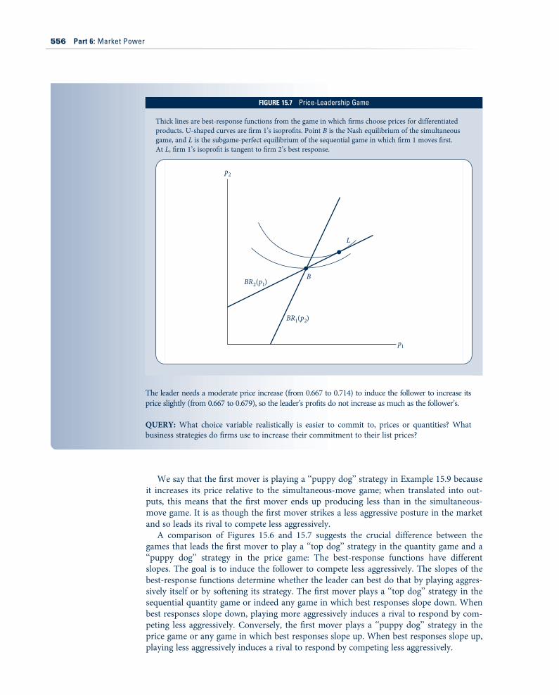
We say that the first mover is playing a ‘‘puppy dog’’ strategy in Example 15.9 becauseit increases its price relative to the simultaneous-move game; when translated into out-puts, this means that the first mover ends up producing less than in the simultaneous-move game. It is as though the first mover strikes a less aggressive posture in the marketand so leads its rival to compete less aggressively.

A comparison of Figures 15.6 and 15.7 suggests the crucial difference between thegames that leads the first mover to play a ‘‘top dog’’ strategy in the quantity game and a‘‘puppy dog’’ strategy in the price game: The best-response functions have differentslopes. The goal is to induce the follower to compete less aggressively. The slopes of thebest-response functions determine whether the leader can best do that by playing aggres-sively itself or by softening its strategy. The first mover plays a ‘‘top dog’’ strategy in thesequential quantity game or indeed any game in which best responses slope down. Whenbest responses slope down, playing more aggressively induces a rival to respond by com-peting less aggressively. Conversely, the first mover plays a ‘‘puppy dog’’ strategy in theprice game or any game in which best responses slope up. When best responses slope up,playing less aggressively induces a rival to respond by competing less aggressively.

The leader needs a moderate price increase (from 0.667 to 0.714) to induce the follower to increase itsprice slightly (from 0.667 to 0.679), so the leader’s profits do not increase as much as the follower’s.

QUERY: What choice variable realistically is easier to commit to, prices or quantities? Whatbusiness strategies do firms use to increase their commitment to their list prices?

FIGURE 15.715Price-Leadership Game

Thick lines are best-response functions from the game in which firms choose prices for differentiatedproducts. U-shaped curves are firm 1’s isoprofits. Point B is the Nash equilibrium of the simultaneousgame, and L is the subgame-perfect equilibrium of the sequential game in which firm 1 moves first.At L, firm 1’s isoprofit is tangent to firm 2’s best response.

p2

BR1(p2)

BR2(p1)B

L

p1


Therefore, knowing the slope of firms’ best responses provides considerable insight intothe sort of strategies firms will choose if they have commitment power. The Extensions atthe end of this chapter provide further technical details, including shortcuts for determin-ing the slope of a firm’s best-response function just by looking at its profit function.

Strategic Entry DeterrenceWe saw that, by committing to an action, a first mover may be able to manipulate thesecond mover into being a less aggressive competitor. In this section we will see that thefirst mover may be able to prevent the entry of the second mover entirely, leaving the firstmover as the sole firm in the market. In this case, the firm may not behave as an uncon-strained monopolist because it may have distorted its actions to fend off the rival’s entry.

In deciding whether to deter the second mover’s entry, the first mover must weigh thecosts and benefits relative to accommodating entry—that is, allowing entry to happen.Accommodating entry does not mean behaving nonstrategically. The first mover wouldmove off its best-response function to manipulate the second mover into being less com-petitive, as described in the previous section. The cost of deterring entry is that the firstmover would have to move off its best-response function even further than it would if itaccommodates entry. The benefit is that it operates alone in the market and has marketdemand to itself. Deterring entry is relatively easy for the first mover if the second movermust pay a substantial sunk cost to enter the market.

EXAMPLE 15.10 Deterring Entry of a Natural Spring

Recall Example 15.8, where two natural-spring owners choose outputs sequentially. We now addan entry stage: In particular, after observing firm 1’s initial quantity choice, firm 2 decideswhether to enter the market. Entry requires the expenditure of sunk cost K2, after which firm 2can choose output. Market demand and cost are as in Example 15.8. To simplify thecalculations, we will take the specific numerical values a ! 120 and c ! 0 [implying that inversedemand is P(Q) ! 120 $ Q, and that production is costless]. To further simplify, we willabstract from firm 1’s entry decision and assume that it has already sunk any cost needed toenter before the start of the game. We will look for conditions under which firm 1 prefers todeter rather than accommodate firm 2’s entry.

Accommodating entry. Start by computing firm 1’s profit if it accommodates firm 2’s entry,denoted pacc

1 . This has already been done in Example 15.8, in which there was no issue of deterringfirm 2’s entry. There we found firm 1’s equilibrium output to be (a$ c)=2 ! qacc1 and its profit tobe (a$ c)2=8 ! pacc

1 . Substituting the specific numerical values a ! 120 and c ! 0, we haveqacc1 ! 60 and pacc

1 ! (120$ 0)2=8 ! 1,800.

Deterring entry. Next, compute firm 1’s profit if it deters firm 2’s entry, denoted pdet1 . To

deter entry, firm 1 needs to produce an amount qdet1 high enough that, even if firm 2 bestresponds to qdet1 , it cannot earn enough profit to cover its sunk cost K2. We know from Equation15.58 that firm 2’s best-response function is

q2 !120$ q1

2: (15:63)

Substituting for q2 in firm 2’s profit function (Equation 15.7) and simplifying gives

p2 !120$ qdet1

2

" #2

$ K2: (15:64)


A real-world example of overproduction (or overcapacity) to deter entry is providedby the 1945 antitrust case against Alcoa, a U.S. aluminum manufacturer. A U.S. federalcourt ruled that Alcoa maintained much higher capacity than was needed to serve themarket as a strategy to deter rivals’ entry, and it held that Alcoa was in violation of anti-trust laws.

To recap what we have learned in the last two sections: with quantity competition, thefirst mover plays a ‘‘top dog’’ strategy regardless of whether it deters or accommodatesthe second mover’s entry. True, the entry-deterring strategy is more aggressive than theentry-accommodating one, but this difference is one of degree rather than kind. However,with price competition (as in Example 15.9), the first mover’s entry-deterring strategywould differ in kind from its entry-accommodating strategy. It would play a ‘‘puppy dog’’

Setting firm 2’s profit in Equation 15.64 equal to 0 and solving yields

qdet1 ! 120$ 2(((((K2p

; (15:65)

qdet1 is the firm 1 output needed to keep firm 2 out of the market. At this output level, firm 1’sprofit is

pdet1 ! 2

(((((K2p

120$ 2(((((K2p) *

, (15:66)

which we found by substituting qdet1 , a ! 120, and c ! 0 into firm 1’s profit function fromEquation 15.7. We also set q2 ! 0 because, if firm 1 is successful in deterring entry, it operatesalone in the market.

Comparison. The final step is to juxtapose p acc1 and p det

1 to find the condition under whichfirm 1 prefers deterring to accommodating entry. To simplify the algebra, let x ! 2

(((((K2p

. Thenpdet1 ! pacc

1 if

x2 $ 120x ' 1,800 ! 0: (15:67)

Applying the quadratic formula yields

x ! 120+(((((((((((7,200p

2: (15:68)

Taking the smaller root (because we will be looking for a minimum threshold), we have x ! 17.6(rounding to the nearest decimal). Substituting x ! 17.6 into x ! 2

(((((K2p

and solving for K2

yields

K2 !x2

$ %2! 17:6

2

" #2

* 77: (15:69)

If K2 ! 77, then entry is so cheap for firm 2 that firm 1 would have to increase its output all theway to qdet1 ! 102 in order to deter entry. This is a significant distortion above what it wouldproduce when accommodating entry: qacc1 ! 60. If K2 < 77, then the output distortion needed todeter entry wastes so much profit that firm 1 prefers to accommodate entry. If K2 > 77, outputneed not be distorted as much to deter entry; thus, firm 1 prefers to deter entry.

QUERY: Suppose the first mover must pay the same entry cost as the second, K1 ! K2 ! K.Suppose further that K is high enough that the first mover prefers to deter rather thanaccommodate the second mover’s entry. Would this sunk cost not be high enough to keep thefirst mover out of the market, too? Why or why not?


strategy if it wished to accommodate entry because this is how it manipulates the secondmover into playing less aggressively. It plays a ‘‘top dog’’ strategy of lowering its price rel-ative to the simultaneous game if it wants to deter entry. Two general principles emerge.

• Entry deterrence is always accomplished by a ‘‘top dog’’ strategy whether competitionis in quantities or prices, or (more generally) whether best-response functions slopedown or up. The first mover simply wants to create an inhospitable environment forthe second mover.

• If firm 1 wants to accommodate entry, whether it should play a ‘‘puppy dog’’ or ‘‘topdog’’ strategy depends on the nature of competition—in particular, on the slope ofthe best-response functions.

SignalingThe preceding sections have shown that the first mover’s ability to commit may afford ita big strategic advantage. In this section we will analyze another possible first-moveradvantage: the ability to signal. If the second mover has incomplete information aboutmarket conditions (e.g., costs, demand), then it may try to learn about these conditionsby observing how the first mover behaves. The first mover may try to distort its actionsto manipulate what the second learns. The analysis in this section is closely tied to thematerial on signaling games in Chapter 8, and the reader may want to review that mate-rial before proceeding with this section.

The ability to signal may be a plausible benefit of being a first mover in some settingsin which the benefit we studied earlier—commitment—is implausible. For example, inindustries where the capital equipment is readily adapted to manufacture other products,costs are not very ‘‘sunk’’; thus, capacity commitments may not be especially credible.The first mover can reduce its capacity with little loss. For another example, the price–leadership game involved a commitment to price. It is hard to see what sunk costs areinvolved in setting a price and thus what commitment value it has.15 Yet even in theabsence of commitment value, prices may have strategic, signaling value.

Entry-deterrence modelConsider the incomplete information game in Figure 15.8. The game involves a firstmover (firm 1) and a second mover (firm 2) that choose prices for their differentiatedproducts. Firm 1 has private information about its marginal cost, which can take on oneof two values: high with probability Pr(H) or low with probability Pr(L) ! 1 $ Pr(H). Inperiod 1, firm 1 serves the market alone. At the end of the period, firm 2 observes firm1’s price and decides whether to enter the market. If it enters, it sinks an entry cost K2

and learns the true level of firm 1’s costs; then firms compete as duopolists in the secondperiod, choosing prices for differentiated products as in Example 15.4 or 15.5. (We donot need to be specific about the exact form of demands.) If firm 2 does not enter, itobtains a payoff of zero, and firm 1 again operates alone in the market. Assume there isno discounting between periods.

Firm 2 draws inferences about firm 1’s cost from the price that firm 1 charges in thefirst period. Firm 2 earns more if it competes against the high-cost type because the

15The Query in Example 15.9 asks you to consider reasons why a firm may be able to commit to a price. The firm may gaincommitment power by using contracts (e.g., long-term supply contracts with customers or a most-favored customer clause,which ensures that if the firm lowers price in the future to other customers, then the favored customer gets a rebate on the pricedifference). The firm may advertise a price through an expensive national advertising campaign. The firm may have establisheda valuable reputation as charging ‘‘everyday low prices.’’


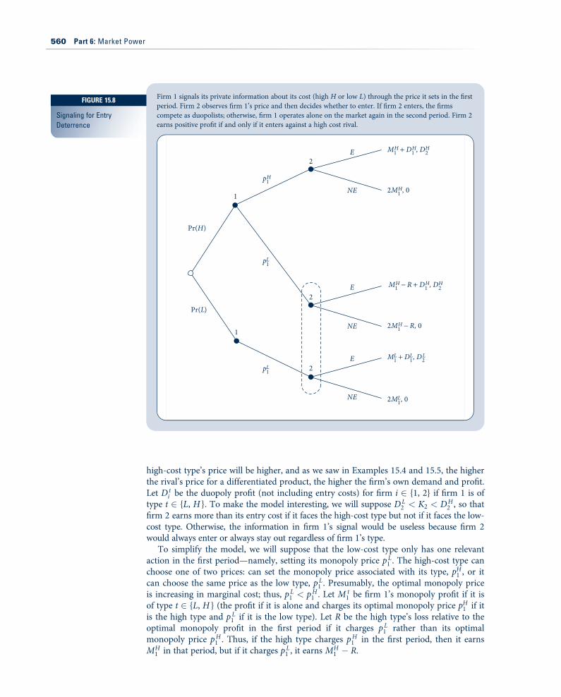
high-cost type’s price will be higher, and as we saw in Examples 15.4 and 15.5, the higherthe rival’s price for a differentiated product, the higher the firm’s own demand and profit.Let Dt

i be the duopoly profit (not including entry costs) for firm i 2 {1, 2} if firm 1 is oftype t 2 {L, H }. To make the model interesting, we will suppose DL

2 < K2 < DH2 , so that

firm 2 earns more than its entry cost if it faces the high-cost type but not if it faces the low-cost type. Otherwise, the information in firm 1’s signal would be useless because firm 2would always enter or always stay out regardless of firm 1’s type.

To simplify the model, we will suppose that the low-cost type only has one relevantaction in the first period—namely, setting its monopoly price pL

1 . The high-cost type canchoose one of two prices: can set the monopoly price associated with its type, pH1 , or itcan choose the same price as the low type, pL

1 . Presumably, the optimal monopoly priceis increasing in marginal cost; thus, pL

1 < pH1 . Let Mt

1 be firm 1’s monopoly profit if it isof type t 2 {L, H } (the profit if it is alone and charges its optimal monopoly price pH1 if itis the high type and pL

1 if it is the low type). Let R be the high type’s loss relative to theoptimal monopoly profit in the first period if it charges pL

1 rather than its optimalmonopoly price pH

1 . Thus, if the high type charges pH1 in the first period, then it earns

MH1 in that period, but if it charges pL

1 , it earns MH1 $ R.

Firm 1 signals its private information about its cost (high H or low L) through the price it sets in the firstperiod. Firm 2 observes firm 1’s price and then decides whether to enter. If firm 2 enters, the firmscompete as duopolists; otherwise, firm 1 operates alone on the market again in the second period. Firm 2earns positive profit if and only if it enters against a high cost rival.

E

E

E

NE

NE

NE

1

2

Pr(L)

Pr(H)

M1H + D1

H, D2H

M1H ! R + D1

H, D2H

M1L + D1

L, D2L

2M1H ! R, 0

2M1L, 0

2M1H, 0

p1H

p1L

p1L

2

2

1

FIGURE 15.8

Signaling for EntryDeterrence


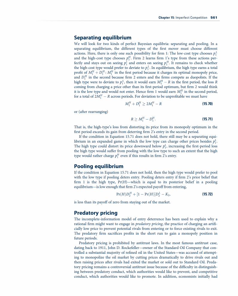
Separating equilibriumWe will look for two kinds of perfect Bayesian equilibria: separating and pooling. In aseparating equilibrium, the different types of the first mover must choose differentactions. Here, there is only one such possibility for firm 1: The low-cost type chooses pL

1and the high-cost type chooses pH1 . Firm 2 learns firm 1’s type from these actions per-fectly and stays out on seeing p11 and enters on seeing pH

1 . It remains to check whetherthe high-cost type would prefer to deviate to pL

1 . In equilibrium, the high type earns a totalprofit of MH

1 ' DH1 : MH

1 in the first period because it charges its optimal monopoly price,and DH

1 in the second because firm 2 enters and the firms compete as duopolists. If thehigh type were to deviate to pL

1 , then it would earn MH1 $ R in the first period, the loss R

coming from charging a price other than its first-period optimum, but firm 2 would thinkit is the low type and would not enter. Hence firm 1 would earn MH

1 in the second period,for a total of 2MH

1 $ R across periods. For deviation to be unprofitable we must have

MH1 ' DH

1 % 2MH1 $ R (15:70)

or (after rearranging)

R % MH1 $ DH

1 : (15:71)

That is, the high-type’s loss from distorting its price from its monopoly optimum in thefirst period exceeds its gain from deterring firm 2’s entry in the second period.

If the condition in Equation 15.71 does not hold, there still may be a separating equi-librium in an expanded game in which the low type can charge other prices besides pL1 .The high type could distort its price downward below pL1 , increasing the first-period lossthe high type would suffer from pooling with the low type to such an extent that the hightype would rather charge pH1 even if this results in firm 2’s entry.

Pooling equilibriumIf the condition in Equation 15.71 does not hold, then the high type would prefer to poolwith the low type if pooling deters entry. Pooling deters entry if firm 2’s prior belief thatfirm 1 is the high type, Pr(H)—which is equal to its posterior belief in a poolingequilibrium—is low enough that firm 2’s expected payoff from entering,

Pr(H)DH2 ' ,1$ Pr(H)-DL

2 $ K2, (15:72)

is less than its payoff of zero from staying out of the market.

Predatory pricingThe incomplete-information model of entry deterrence has been used to explain why arational firm might want to engage in predatory pricing, the practice of charging an artifi-cially low price to prevent potential rivals from entering or to force existing rivals to exit.The predatory firm sacrifices profits in the short run to gain a monopoly position infuture periods.

Predatory pricing is prohibited by antitrust laws. In the most famous antitrust case,dating back to 1911, John D. Rockefeller—owner of the Standard Oil Company that con-trolled a substantial majority of refined oil in the United States—was accused of attempt-ing to monopolize the oil market by cutting prices dramatically to drive rivals out andthen raising prices after rivals had exited the market or sold out to Standard Oil. Preda-tory pricing remains a controversial antitrust issue because of the difficulty in distinguish-ing between predatory conduct, which authorities would like to prevent, and competitiveconduct, which authorities would like to promote. In addition, economists initially had


trouble developing game-theoretic models in which predatory pricing is rational andcredible.

Suitably interpreted, predatory pricing may emerge as a rational strategy in theincomplete-information model of entry deterrence. Predatory pricing can show up in aseparating equilibrium—in particular, in the expanded model where the low-cost typecan separate only by reducing price below its monopoly optimum. Total welfare isactually higher in this separating equilibrium than it would be in its full-informationcounterpart. Firm 2’s entry decision is the same in both outcomes, but the low-cost type’sprice may be lower (to signal its type) in the predatory outcome.

Predatory pricing can also show up in a pooling equilibrium. In this case it is thehigh-cost type that charges an artificially low price, pricing below its first-period opti-mum to keep firm 2 out of the market. Whether social welfare is lower in the poolingequilibrium than in a full-information setting is unclear. In the first period, price islower (and total welfare presumably higher) in the pooling equilibrium than in a full-information setting. On the other hand, deterring firm 2’s entry results in higher second-period prices and lower welfare. Weighing the first-period gain against the second-periodloss would require detailed knowledge of demand curves, discount factors, and so forth.

The incomplete-information model of entry deterrence is not the only model of preda-tory pricing that economists have developed. Another model involves frictions in themarket for financial capital that stem perhaps from informational problems (betweenborrowers and lenders) of the sort we will discuss in Chapter 18. With limits on borrow-ing, firms may only have limited resources to ‘‘make a go’’ in a market. A larger firm mayforce financially strapped rivals to endure losses until their resources are exhausted andthey are forced to exit the market.

How Many Firms Enter?To this point, we have taken the number of firms in the market as given, often assumingthat there are at most two firms (as in Examples 15.1, 15.3, and 15.10). We did allow for ageneral number of firms, n, in some of our analysis (as in Examples 15.3 and 15.7) but weresilent about how this number n was determined. In this section, we provide a game-theoretic analysis of the number of firms by introducing a first stage in which a large numberof potential entrants can each choose whether to enter. We will abstract from first-moveradvantages, entry deterrence, and other strategic considerations by assuming that firmsmake their entry decisions simultaneously. Strategic considerations are interesting and im-portant, but we have already developed some insights into strategic considerations from theprevious sections and—by abstracting from them—we can simplify the analysis here.

Barriers to entryFor the market to be oligopolistic with a finite number of firms rather than perfectly com-petitive with an infinite number of infinitesimal firms, some factors, called barriers toentry, must eventually make entry unattractive or impossible. We discussed many of thesefactors at length in the previous chapter on monopoly. If a sunk cost is required to enterthe market, then—even if firms can freely choose whether to enter—only a limited num-ber of firms will choose to enter in equilibrium because competition among more thanthat number would drive profits below the level needed to recoup the sunk entry cost.Government intervention in the form of patents or licensing requirements may preventfirms from entering even if it would be profitable for them to do so.

Some of the new concepts discussed in this chapter may introduce additional barriersto entry. Search costs may prevent consumers from finding new entrants with lower


prices and/or higher quality than existing firms. Product differentiation may raise entrybarriers because of strong brand loyalty. Existing firms may bolster brand loyalty throughexpensive advertising campaigns, and softening this brand loyalty may require entrantsto conduct similarly expensive advertising campaigns. Existing firms may take other stra-tegic measures to deter entry, such as committing to a high capacity or output level,engaging in predatory pricing, or other measures discussed in previous sections.

Long-run equilibriumConsider the following game-theoretic model of entry in the long run. A large number ofsymmetric firms are potential entrants into a market. Firms make their entry decisionssimultaneously. Entry requires the expenditure of sunk cost K. Let n be the number offirms that decide to enter. In the next stage, the n firms engage in some form of competi-tion over a sequence of periods during which they earn the present discounted value ofsome constant profit stream. To simplify, we will usually collapse the sequence of periodsof competition into a single period. Let g (n) be the profit earned by an individual firm inthis competition subgame [not including the sunk cost, so g (n) is a gross profit]. Presum-ably, the more firms in the market, the more competitive the market is and the less anindividual firm earns, so g 0(n) < 0.

We will look for a subgame-perfect equilibrium in pure strategies.16 This will be thenumber of firms, n", satisfying two conditions. First, the n" entering firms earn enough tocover their entry cost: g (n") % K. Otherwise, at least one of them would have preferred tohave deviated to not entering. Second, an additional firm cannot earn enough to cover itsentry cost: g (n" ' 1) # K. Otherwise, a firm that remained out of the market could haveprofitably deviated by entering. Given that g 0(n) < 0, we can put these two conditions to-gether and say that n" is the greatest integer satisfying g (n") % K.

This condition is reminiscent of the zero-profit condition for long-run equilibriumunder perfect competition. The slight nuance here is that active firms are allowed to earnpositive profits. Especially if K is large relative to the size of the market, there may onlybe a few long-run entrants (thus, the market looks like a canonical oligopoly) earning wellabove what they need to cover their sunk costs, yet an additional firm does not enterbecause its entry would depress individual profit enough that the entrant could not coverits large sunk cost.

Is the long-run equilibrium efficient? Does the oligopoly involve too few or too manyfirms relative to what a benevolent social planner would choose for the market? Supposethe social planner can choose the number of firms (restricting entry through licenses andpromoting entry through subsidizing the entry cost) but cannot regulate prices or othercompetitive conduct of the firms once in the market. The social planner would choose nto maximize

CS(n) ' ng(n) $ nK; (15:73)

where CS(n) is equilibrium consumer surplus in an oligopoly with n firms, ng(n) is totalequilibrium profit (gross of sunk entry costs) across all firms, and nK is the total expendi-ture on sunk entry costs. Let n"" be the social planner’s optimum.

In general, the long-run equilibrium number of firms, n", may be greater or less thanthe social optimum, n"", depending on two offsetting effects: the appropriability effectand the business-stealing effect.

16A symmetric mixed-strategy equilibrium also exists in which sometimes more and sometimes fewer firms enter than can covertheir sunk costs. There are multiple pure-strategy equilibria depending on the identity of the n" entrants, but n" is uniquelyidentified.


• The social planner takes account of the benefit of increased consumer surplus fromlower prices, but firms do not appropriate consumer surplus and so do not take intoaccount this benefit. This appropriability effect would lead a social planner to choosemore entry than in the long-run equilibrium: n"" > n".

• Working in the opposite direction is that entry causes the profits of existing firms todecrease, as indicated by the derivative g 0(n) < 0. Entry increases the competitivenessof the market, destroying some of firms’ profits. In addition, the entrant ‘‘steals’’ somemarket share from existing firms—hence the term business-stealing effect. The mar-ginal firm does not take other firms’ loss in profits when making its entry decision,whereas the social planner would. The business-stealing effect biases long-run equilib-rium toward more entry than a social planner would choose: n"" < n".

Depending on the functional forms for demand and costs, the appropriability effect dom-inates in some cases, and there is less entry in long-run equilibrium than is efficient. Inother cases, the business-stealing dominates, and there is more entry in long-run equilib-rium than is efficient, as in Example 15.11.

EXAMPLE 15.11 Cournot in the Long Run

Long-run equilibrium. Return to Example 15.3 of a Cournot oligopoly. We will determinethe long-run equilibrium number of firms in the market. Let K be the sunk cost a firm must payto enter the market in an initial entry stage. Suppose there is one period of Cournot competitionafter entry. To further simplify the calculations, assume that a ! 1 and c ! 0. Substituting thesevalues back into Example 15.3, we have that an individual firm’s gross profit is

g(n) ! 1n' 1

" #2

: (15:74)

The long-run equilibrium number of firms is the greatest integer n" satisfying g (n") % K.Ignoring integer problems, n" satisfies

n" ! 1((((Kp $ 1: (15:75)

Social planner’s problem. We first compute the individual terms in the social planner’sobjective function (Equation 15.73). Consumer surplus equals the area of the shaded triangle inFigure 15.9, which, using the formula for the area of a triangle, is

CS(n) ! 12Q(n),a$ P(n)- ! n 2

2(n' 1)2; (15:76)

here the last equality comes from substituting for price and quantity from Equations 15.18 and15.19. Total profits for all firms (gross of sunk costs) equal the area of the shaded rectangle:

ng(n) ! Q(n)P(n) ! n

(n' 1)2: (15:77)

Substituting from Equations 15.76 and 15.77 into the social planner’s objective function(Equation 15.73) gives

n 2

2(n' 1)2' n

(n' 1)2$ nK: (15:78)

After removing positive constants, the first-order condition with respect to n is

1$ K(n' 1)3 ! 0, (15:79)


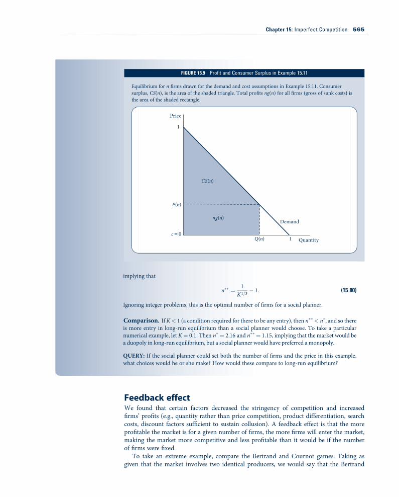
Feedback effectWe found that certain factors decreased the stringency of competition and increasedfirms’ profits (e.g., quantity rather than price competition, product differentiation, searchcosts, discount factors sufficient to sustain collusion). A feedback effect is that the moreprofitable the market is for a given number of firms, the more firms will enter the market,making the market more competitive and less profitable than it would be if the numberof firms were fixed.

To take an extreme example, compare the Bertrand and Cournot games. Taking asgiven that the market involves two identical producers, we would say that the Bertrand

implying that

n"" ! 1K1=3

$ 1: (15:80)

Ignoring integer problems, this is the optimal number of firms for a social planner.

Comparison. IfK< 1 (a condition required for there to be any entry), then n""< n", and so thereis more entry in long-run equilibrium than a social planner would choose. To take a particularnumerical example, let K! 0.1. Then n" ! 2.16 and n"" ! 1.15, implying that the market would bea duopoly in long-run equilibrium, but a social planner would have preferred amonopoly.

QUERY: If the social planner could set both the number of firms and the price in this example,what choices would he or she make? How would these compare to long-run equilibrium?

FIGURE 15.915Profit and Consumer Surplus in Example 15.11

Equilibrium for n firms drawn for the demand and cost assumptions in Example 15.11. Consumersurplus, CS(n), is the area of the shaded triangle. Total profits ng(n) for all firms (gross of sunk costs) isthe area of the shaded rectangle.

Price

1

Q(n)

P(n)

1

CS(n)

ng(n)

c = 0Quantity

Demand


game is much more competitive and less profitable than the Cournot game. This conclu-sion would be reversed if firms facing a sunk entry cost were allowed to make rationalentry decisions. Only one firm would choose to enter the Bertrand market. A second firmwould drive gross profit to zero, and so its entry cost would not be covered. The long-runequilibrium outcome would involve a monopolist and thus the highest prices and profitspossible, exactly the opposite of our conclusions when the number of firms was fixed! Onthe other hand, the Cournot market may have space for several entrants driving pricesand profits below their monopoly levels in the Bertrand market.

The moderating effect of entry should lead economists to be careful when drawingconclusions about oligopoly outcomes. Product differentiation, search costs, collusion,and other factors may reduce competition and increase profits in the short run, butthey may also lead to increased entry and competition in the long run and thus haveambiguous effects overall on prices and profits. Perhaps the only truly robust conclu-sions about prices and profits in the long run involve sunk costs. Greater sunk costsconstrain entry even in the long run, so we can confidently say that prices and profitswill tend to be higher in industries requiring higher sunk costs (as a percentage ofsales) to enter.17

InnovationAt the end of the previous chapter, we asked which market structure—monopoly or perfectcompetition—leads to more innovation in new products and cost-reducing processes. Ifmonopoly is more innovative, will the long-run benefits of innovation offset the short-rundeadweight loss of monopoly? The same questions can be asked in the context of oligop-oly. Do concentrated market structures, with few firms perhaps charging high prices, pro-vide better incentives for innovation? Which is more innovative, a large or a small firm?An established firm or an entrant? Answers to these questions can help inform policytoward mergers, entry regulation, and small-firm subsidies.

As we will see with the aid of some simple models, there is no definite answer as towhat level of concentration is best for long-run total welfare. We will derive some generaltrade-offs, but quantifying these trade-offs to determine whether a particular marketwould be more innovative if it were concentrated or unconcentrated will depend on thenature of competition for innovation, the nature of competition for consumers, and thespecification of demand and cost functions. The same can be said for determining whatfirm size or age is most innovative.

The models we introduce here are of product innovations, the invention of a product(e.g., plasma televisions) that did not exist before. Another class of innovations is that ofprocess innovations, which reduce the cost of producing existing products—for example,the use of robot technology in automobile manufacture.

Monopoly on innovationBegin by supposing that only a single firm, call it firm 1, has the capacity to innovate. Forexample, a pharmaceutical manufacturer may have an idea for a malaria vaccine thatno other firm is aware of. How much would the firm be willing to complete research anddevelopment for the vaccine and to test it with large-scale clinical trials? How does thiswillingness to spend (which we will take as a measure of the innovativeness of the firm)depend on concentration of firms in the market?

17For more on robust conclusions regarding industry structure and competitiveness, see J. Sutton, Sunk Costs and Market Struc-ture (Cambridge, MA: MIT Press, 1991).


Suppose first that there is currently no other vaccine available for malaria. If firm 1successfully develops the vaccine, then it will be a monopolist. Letting GM be themonopoly profit, firm 1 would be willing to spend as much as GM to develop the vaccine.Next, to examine the case of a less concentrated market, suppose that another firm (firm 2)already has a vaccine on the market for which firm 1’s would be a therapeutic substitute.If firm 1 also develops its vaccine, the firms compete as duopolists. Let pD be the duop-oly profit. In a Bertrand model with identical products, pD ! 0, but pD > 0 in othermodels—for example, models involving quantity competition or collusion. Firm 1 wouldbe willing to spend as much as pD to develop the vaccine in this case. Comparing thetwo cases, because GM > pD, it follows that firm 1 would be willing to spend more(and, by this measure, would be more innovative) in a more concentrated market. Thegeneral principle here can be labeled a dissipation effect: Competition dissipates some ofthe profit from innovation and thus reduces incentives to innovate. The dissipationeffect is part of the rationale behind the patent system. A patent grants monopoly rightsto an inventor, intentionally restricting competition to ensure higher profits and greaterinnovation incentives.

Another comparison that can be made is to see which firm, 1 or 2, has more of an in-centive to innovate given that it has a monopoly on the initial idea. Firm 1 is initiallyout of the market and must develop the new vaccine to enter. Firm 2 is already in themalaria market with its first vaccine but can consider developing a second one as well,which we will continue to assume is a perfect substitute. As shown in the previous para-graph, firm 1 would be willing to pay up to pD for the innovation. Firm 2 would not bewilling to pay anything because it is currently a monopolist in the malaria vaccine mar-ket and would continue as a monopolist whether or not it developed the second medi-cine. (Crucial to this conclusion is that the firm with the initial idea can decline todevelop it but still not worry that the other firm will take the idea; we will change thisassumption in the next subsection.) Therefore, the potential competitor (firm 1) is moreinnovative by our measure than the existing monopolist (firm 2). The general principlehere has been labeled a replacement effect: Firms gain less incremental profit and thushave less incentive to innovate if the new product replaces an existing product alreadymaking profit than if the firm is a new entrant in the market. The replacement effectcan explain turnover in certain industries where old firms become increasingly conserva-tive and are eventually displaced by innovative and quickly growing startups, as Micro-soft displaced IBM as the dominant company in the computer industry and as Googlenow threatens to replace Microsoft.

Competition for innovationNew firms are not always more innovative than existing firms. The dissipation effect maycounteract the replacement effect, leading old firms to be more innovative. To see thistrade-off requires yet another variant of the model. Suppose now that more than one firmhas an initial idea for a possible innovation and that they compete to see which can de-velop the idea into a viable product. For example, the idea for a new malaria vaccine mayhave occurred to scientists in two firms’ laboratories at about the same time, and thefirms may engage in a race to see who can produce a viable vaccine from this initial idea.Continue to assume that firm 2 already has a malaria vaccine on the market and that thisnew vaccine would be a perfect substitute for it.

The difference between the models in this and the previous section is that if firm 2does not win the race to develop the idea, then the idea does not simply fall by the way-side but rather is developed by the competitor, firm 1. Firm 2 has an incentive to win theinnovation competition to prevent firm 1 from becoming a competitor. Formally, if firm 1wins the innovation competition, then it enters the market and is a competitor with firm 2,


earning duopoly profit pD. As we have repeatedly seen, this is the maximum that firm 1would pay for the innovation. Firm 2’s profit is GM if it wins the competition for the inno-vation but pD if it loses and firm 1 wins. Firm 2 would pay up to the difference, GM $ pD,for the innovation. If GM > 2pD—that is, if industry profit under a monopoly is greaterthan under a duopoly, which it is when some of the monopoly profit is dissipated by duop-oly competition—then GM $ pD > pD, and firm 2 will have more incentive to innovatethan firm 1.

This model explains the puzzling phenomenon of dominant firms filing for ‘‘sleeping pat-ents’’: patents that are never implemented. Dominant firms have a substantial incentive—aswe have seen, possibly greater than entrants’—to file for patents to prevent entry and preservetheir dominant position. Whereas the replacement effect may lead to turnover in the marketand innovation by new firms, the dissipation effect may help preserve the position of domi-nant firms and retard the pace of innovation.

SUMMARY

Many markets fall between the polar extremes of perfectcompetition and monopoly. In such imperfectly competitivemarkets, determining market price and quantity is compli-cated because equilibrium involves strategic interactionamong the firms. In this chapter, we used the tools of gametheory developed in Chapter 8 to study strategic interactionin oligopoly markets. We first analyzed oligopoly firms’short-run choices such as prices and quantities and thenwent on to analyze firms’ longer-run decisions such as prod-uct location, innovation, entry, and the deterrence of entry.We found that seemingly small changes in modelingassumptions may lead to big changes in equilibrium out-comes. Therefore, predicting behavior in oligopoly marketsmay be difficult based on theory alone and may requireknowledge of particular industries and careful empiricalanalysis. Still, some general principles did emerge from ourtheoretical analysis that aid in understanding oligopolymarkets.

• One of the most basic oligopoly models, the Bertrandmodel involves two identical firms that set pricessimultaneously. The equilibrium resulted in the Ber-trand paradox: Even though the oligopoly is the mostconcentrated possible, firms behave as perfect competi-tors, pricing at marginal cost and earning zero profit.

• The Bertrand paradox is not the inevitable outcome inan oligopoly but can be escaped by changing assump-tions underlying the Bertrand model—for example,allowing for quantity competition, differentiated prod-ucts, search costs, capacity constraints, or repeated playleading to collusion.

• As in the Prisoners’ Dilemma, firms could profit bycoordinating on a less competitive outcome, but thisoutcome will be unstable unless firms can explicitly

collude by forming a legal cartel or tacitly collude in arepeated game.

• For tacit collusion to sustain supercompetitive profits,firms must be patient enough that the loss from a pricewar in future periods to punish undercutting exceedsthe benefit from undercutting in the current period.

• Whereas a nonstrategic monopolist prefers flexibility torespond to changing market conditions, a strategic oli-gopolist may prefer to commit to a single choice. Thefirm can commit to the choice if it involves a sunk costthat cannot be recovered if the choice is later reversed.

• A first mover can gain an advantage by committing toa different action from what it would choose in theNash equilibrium of the simultaneous game. To deterentry, the first mover should commit to reducing theentrant’s profits using an aggressive ‘‘top dog’’ strategy(high output or low price). If it does not deter entry,the first mover should commit to a strategy leading itsrival to compete less aggressively. This is sometimes a‘‘top dog’’ and sometimes a ‘‘puppy dog’’ strategy,depending on the slope of firms’ best responses.

• Holding the number of firms in an oligopoly constantin the short run, the introduction of a factor that soft-ens competition (e.g., product differentiation, searchcosts, collusion) will increase firms’ profit, but an off-setting effect in the long run is that entry—which tendsto reduce oligopoly profit—will be more attractive.

• Innovation may be even more important than lowprices for total welfare in the long run. Determiningwhich oligopoly structure is the most innovative is dif-ficult because offsetting effects (dissipation and replace-ment) are involved.


imperfect competition

Documents