Electronic copy available at: http://ssrn.com/abstract=603721

Imperfect competition in �nancial

markets and capital structure�

Sergei Gurievy Dmitriy Kvasovz

August 2007

�We are grateful to Philippe Aghion, Sudipto Bhattacharya, Patrick Bolton, Bengt Holmstrom,

Michael Riordan, Sergey Stepanov, Lars Stole, and Dimitri Vayanos, and seminar and conference par-

ticipants in Helsinki, Moscow, and Wellington for helpful comments. The �rst author acknowledges the

hospitality of Princeton University where the work has been started.yNew Economic School and CEPR. E-mail: sguriev@nes.ruzUniversity of Auckland. E-mail: d.kvasov@auckland.ac.nz

1

Electronic copy available at: http://ssrn.com/abstract=603721

Imperfect competition in �nancial markets and capital structure

Abstract.

We consider a model of corporate �nance with imperfectly competitive �nancial inter-

mediaries. Firms can �nance projects either via debt or via equity. Because of asymmetric

information about �rms�growth opportunities, equity �nancing involves a dilution cost.

Nevertheless, equity emerges in equilibrium whenever �nancial intermediaries have suf-

�cient market power. In the latter case, best �rms issue debt while the less pro�table

�rms are equity-�nanced. We also show that strategic interaction between oligopolistic

intermediaries results in multiple equilibria. If one intermediary chooses to buy more

debt, the price of debt decreases, so the best equity-issuing �rms switch from equity to

debt �nancing. This in turn decreases average quality of equity-�nanced pool, so other

intermediaries also shift towards more debt.

Keywords: capital structure, pecking order theory of �nance, oligopoly in �nancial

markets, second degree price discrimination

JEL Codes: D43, G32, L13

1 Introduction

The choice of capital structure is one of the central issues in corporate �nance. The

cornerstone paper by Modigliani and Miller (1958) established that capital structure is

irrelevant as long as �nancial markets are perfect. As �nancing decisions do matter in

the real world, corporate �nance literature has come up with a number of theories which

show how various imperfections explain the observed patterns of capital structure. These

explanations have mostly concentrated on the imperfections on the side of the �rm. In

these theories, the optimal capital structure minimizes the costs borne by investors as a

result of taxes, asymmetric information, con�icts of interest between management and

shareholders etc. Since the �nancial markets are assumed to be perfectly competitive,

these costs are passed back to the �rm in the form of a higher cost of capital thus providing

incentives to choose an optimal capital structure.

In this paper, we study how the capital structure is a¤ected by an imperfection on the

side of �nancial markets. We assume that �nancial intermediaries have market power.

There are many reasons to believe that �nancial markets are not perfectly competitive.

Financial services require reputational capital; information accumulation and processing

also create economies of scale and barriers to entry (Dell�Arricia et al., 1999). Morrison

and Wilhelm (2007) argue that the increasing codi�cation of certain investment banking

activities have recently resulted in even greater scale economies in the investment banking

business.

Not surprisingly, after the Glass-Steagall Act was repealed in 1999, the global �nancial

market has been increasingly dominated by a few �global, universal banks of new genera-

tion�(Calomiris, 2002) that provide both commercial and investment banking services (as

well as other �nancial services) as well as command a substantial market share in virtually

all �nancial markets, including debt and equity issues. According to Thomson Financial

(www.thomson.com) nine largest �nancial groups (Goldman Sachs, Lehman Brothers,

Merrill Lynch, Morgan Stanley, Citi, JP Morgan, Credit Suisse, Deutsche Bank, and

UBS) control more than 50% in every major �nancial market; in many markets top �ve

�nancial intermediaries control up to 70% of the market. Morrison and Wilhelm (2007)

cite Securities Data Corporation�s data to show that the top �ve (top ten) banks�share in

the US common stock o¤ering has risen from 38% (62%) in 1970 to 64% (87%) in 2003.

These trends have not been unnoticed by policymakers and academics. In 1999, the US

Department of Justice launched an antitrust investigation on the IPO fees (Smith, 1999).

The academic debate on the collusive nature of IPO fees clustering is not conclusive (see

1

Chen and Ritter, 2000 who argue that the IPO fees clustering around 7% in the US is a

sign of tacit collusion and Torstila (2003) for cross-country evidence and the summary of

the debate); yet, the very nature of this debate suggests that investment banking industry

is not perfectly competitive. This conjecture is also consistent with the legal analysis by

Gri¢ th (2006) who argues that underwriters possess market power and use it for price

discrimination.

Why does imperfect competition matter for capital structure? Once the �nancial

intermediaries behave strategically, the logic of conventional capital structure theories falls

apart. Under perfect competition, the investors�costs are passed onto the �rm because

investors earn zero rents on all �nancial instruments. We still assume that investors are

perfectly competitive, but the intermediaries between investors and �rms are oligopolistic.

In this case, �nancial intermediaries receive positive rents; these rents may di¤er for

debt and equity investments. Since �rms choose capital structure depending on their

growth opportunities, intermediaries can use capital structure as a means of the second

degree price discrimination (similarly to using monetary and barter contracts in Guriev

and Kvassov, 2004). The purpose of discrimination is to extract higher fees from more

pro�table �rms. We �nd that equilibrium capital structure is di¤erent in competitive and

concentrated markets. For expositional clarity, we assume away all possible costs of debt

�nancing. In this case, in line with the pecking order theory, debt crowds out equity as

long as �nancial markets are su¢ ciently competitive. However, as markets become more

concentrated, equity �nancing does emerge in equilibrium. Concentration of market power

results in a substantial wedge between the oligopolistic interest rate and intermediaries�

cost of funds. Hence, there is a pool of �rms that would borrow at rates which are below

the market interest rate on debt but still above intermediaries�cost of funds. In order

to serve these �rms without sacri�cing revenues from lending at a high rate to existing

borrowers, intermediaries use capital structure as a screening device. The better �rms

still prefer debt, while the less pro�table �rms are happy to issue equity. Therefore our

paper is consistent with the recent increase in concentration in investment banking and

the rise of equity issues worldwide in recent years.

What makes our paper more than just another model of capital structure is the study

of strategic interaction that results in multiple equilibria. As we show, these equilibria

di¤er in terms of both capital structure and asset prices even though all agents are fully

rational. This in turn provides a very simple rationale for stock market volatility, bubbles

and crashes without resorting to assumptions on bounded rationality or limits of arbitrage.

2

The intuition for multiplicity of equilibria is the strategic complementarity of portfolio

choices by the �nancial intermediaries.1 Suppose that one intermediary decides to move

from debt to equity. This raises interest rate on debt so that some �rms that used to

borrow can no longer a¤ord debt �nance. These �rms switch to equity which improves

average quality of the pool of equity-�nanced �rms (all debt-�nanced �rms are better than

equity-�nanced ones). This makes equity investment more attractive so other investors

also choose to shift from debt to equity. We show that multiple equilibria do exist for a

range of parameter values.

Our analysis has two kinds of empirical implications. First, ceteris paribus both across

countries and over time, higher concentration of �nancial market power should result in a

greater reliance on equity �nance. Secondly, the stock price volatility is higher for inter-

mediate ranges of concentration. If markets are perfectly competitive, there is a unique

equilibrium where debt �nance prevails; if markets are too concentrated, there is only one

equilibrium with a high share of equity �nancing. Unfortunately, both predictions are hard

to test as there are many other determinants of capital structure that are correlated with

changes in concentration of debt and equity markets. In particular, the cross-country

test of our hypothesis is problematic as legal protection of outside shareholders in the

US results in a widespread use of equity even though the US �nancial markets are very

competitive (La Porta et al., 1998). As for the within-US experience over time, it is

rather consistent with our results: the consolidation of �nancial industry in 1990s was

accompanied by a growth in equity �nance and in higher stock market volatility. In any

case, �nding appropriate instruments or locating a suitable natural experiment remains

a subject for future empirical work.

Related literature. Market concentration is not the only explanation of coexistence of

debt and equity under asymmetric information. In the pecking order literature equity

�nance may emerge in equilibrium either if debt is costly or if information production is

endogenous. In Bolton and Freixas (2000), both bank loans and public debt coexist in

equilibrium with equity. Although equity �nancing involves a dilution cost, it still emerges

in equilibrium since debt �nancing is also costly. Banks need to raise funds themselves and,

therefore, bear intermediation costs, while bond �nancing involves ine¢ cient liquidation.

Since dispersed bondholders cannot overcome the free-rider problem, they are less likely

to be �exible ex post (unlike banks). Again, each �rm chooses the capital structure which

1Our model is an application of Bulow et al.�s multi-market oligopoly model in the case where demands

rather than costs are interrelated across markets (as in Section VI.K of Bulow et al., 1985).

3

is the least costly one for the investors since the perfect competition in �nancial markets

translates investors�costs into a higher cost of capital for the �rm. Other potential costs

of excessive leverage include costs of bankruptcy and agency costs of debt (Bradley et al.,

1984). Cooney and Kalay (1993), consider the case of asymmetric information about both

mean and volatility of the project returns; equity �nance emerges in equilibrium. In Boot

and Thakor (1993) and in Fulghieri and Lukin (2001), equity issues provide incentives for

investors to produce information hence bringing stock price closer to fundamentals and

increasing issuer�s revenues.

Our model is based on the pecking order theory of capital structure (Myers and Ma-

jluf, 1984). There is no consensus in the literature whether the pecking order theory

outperforms the other explanations of capital structure � the trade-o¤ theory and the

agency theory. The empirical literature produces controversial results (see e.g. Myers,

2000, Baker and Wurgler, 2002, Mayer and Sussman, 2004, Welch, 2004, Fama and French

2005). It would probably be safe to say (see e.g. Fama and French, 2002, and Leary and

Roberts, 2007) that a simple pecking order theory is certainly outperformed by the �com-

plex pecking order theory�which incorporates features of the other theories. While we

use the original pecking order theory as a point of reference, our results certainly extend

to more general setups (see Section 4). Moreover, our analysis shows that even the simple

pecking order theory may be consistent with the data once the imperfect competition

in �nancial markets is taken into account. Once the perfect competition assumption is

relaxed, equity is issued even in this simple setup with all potential costs of debt �nancing

assumed away.

While most of the capital structure literature studies perfectly competitive �nancial

markets, there are a few papers that focus on imperfect competition. Petersen and Ra-

jan (1994, 1995) consider a model of a monopolistic creditor that performs better than

competitive market because it is able to form long-term ties and internalize the debtor�s

bene�ts from investment. In many ways, this arrangement is similar to our equity �-

nancing (which also emerges in highly concentrated markets). Faulkender and Petersen

(2006) also focus on the imperfections on the market�s side and show that underleverage

may be related to rationing by lenders rather than to �rms�characteristics. Neither pa-

per, however, considers oligopoly and therefore does not describe the e¤ects of strategic

interactions.

The paper by Degryse et al. (2007) also studies imperfect competition in banking and

focuses on the interaction between organizational structure and the imperfectly competi-

4

tive equilibrium. Our setup is similar but we focus on the interaction between debt and

equity markets (Degryse et al. only consider lending).

There is also a literature on market microstructure (e.g. Brunnermeier, 2001, ch. 3)

that explicitly models the competition between market makers in �nancial markets. Our

setting is most similar to Biais et al. (2000) who consider oligopolistic uninformed market

makers screening informed traders. However, the market microstructure models study

a single �nancial market while we focus on the situation where �nancial intermediaries

interact strategically in two markets (debt and equity) using capital structure to screen

�rms.

Our paper is also related to the literature on bubbles and crashes, as well as the one

on the IPO waves. While our model does not describe bubbles (de�ned as deviations of

stock prices from their fundamental values), we do show that there are multiple equilibria

with di¤erent stock returns and volumes of stock issued; in this respect our paper is sim-

ilar to Allen and Gale (2003) who discuss crises that are driven by endogenous change in

fundamental value per se. Our model provides a rational explanation for the widespread

market timing; the fact that �rms issue equity when stock price is high and repurchase

when low (Baker and Wurgler, 2002) can be explained by multiplicity of equilibria. Also,

our rationale for stock market crashes is somewhat similar to the one in Abreu and Brun-

nermeier (2000) who explain persistent bubbles by coordination failure between rational

arbitragers over time. Our analysis is also related to Asparouhova (2006) who studies

(both theoretically and experimentally) a setting with competitive lending to heteroge-

nous entrepreneurs under asymmetric information on their risks. To screen the borrowers,

the lenders o¤er menues of debt contracts; the experimental results are consistent with

theory predicting non-existence of equilibria for certain parameter values.

The rest of the paper is structured as follows. In Section 2, we set up the model. In

Section 3 we fully characterize the equilibria in a special case where the distribution of

�rms satis�es the monotone hazard rate condition; we show that if market structure is

su¢ ciently concentrated there may be two stable equilibria: one with debt and equity

�nance, and the other one with debt �nance only. We also consider an example with-

out the monotone hazard rate condition where there are multiple equilibria with equity.

Section 4 discusses extensions; in particular, we depart from the Cournot setup and con-

sider Bertrand competition with di¤erentiated goods. Section 5 concludes and describes

empirical implications.

5

2 The model

2.1 The setting

There are two periods: ex ante t = 1 (�nancing and investments) and ex post t = 2

(realization of returns and payo¤s). Discount rates are normalized to 1. There are a �nite

number of investors and a continuum of �rms normalized to 1.

Firms. Each �rm has an individual investment project that requires 1 unit of funds

in the �rst period and brings gross return � in the second period. The return is the �rm�s

private information at the time of �nancing but is publicly observable ex post. The �rms�

types � are distributed on [�; �] with c.d.f. F (�) without mass points. Firms have no cashand, therefore, have to rely on either debt or equity. We rule out a possibility of issuing

both equity and debt (until Section 4).2

Firms act in the interests of their existing shareholders. After production takes place

and payo¤s are realized, �rms are liquidated. The �rms�outside options are normalized

to zero.

Intermediaries. There are N �nancial intermediaries. The intermediaries have unlim-

ited access to investors�funds at a constant cost � (e.g., an interest rate to be paid to the

ultimate providers of funds). The intermediaries can choose how much to invest in bonds

or stocks. The intermediaries have market power and behave strategically; they take into

account the impact of their strategies on the market prices of debt and equity.

It is important to emphasize that continuum of �rms and a �nite number of interme-

diaries does not imply that intermediaries are scarce and projects are in in�nite supply.

On the contrary, the number of projects is limited (normalized to 1), and intermediaries

can bring in an unlimited amount of resources (at a marginal cost �):

Debt. In this model we do not distinguish between bank loans and bonds. The debt

contract is standard: �borrow D in the �rst period, pay back rD in the second period; if

the repayment is not made, the creditors take over the �rm.�The return on debt, r, is

endogenous and is determined in an (imperfectly competitive) market equilibrium model.

We assume that there is an in�nitesimal cost of bankruptcy. If the �rm is indi¤erent

between repaying or undergoing bankruptcy, it always chooses repayment. In the �rst

period, the �rm has no uncertainty about its second-period returns. As a result, the �rm

never borrows more than it can pay back and default on debt never happens.

The �rst-period price of a debt contract that promises to pay the investor $1 is p = 1=r.

2One can assume that each method of �nance may involve a �xed cost, e.g. same for debt and equity.

6

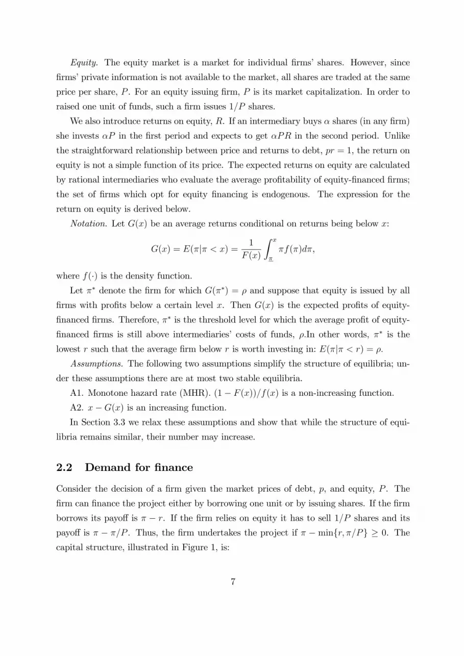
Equity. The equity market is a market for individual �rms�shares. However, since

�rms�private information is not available to the market, all shares are traded at the same

price per share, P . For an equity issuing �rm, P is its market capitalization. In order to

raised one unit of funds, such a �rm issues 1=P shares.

We also introduce returns on equity, R. If an intermediary buys � shares (in any �rm)

she invests �P in the �rst period and expects to get �PR in the second period. Unlike

the straightforward relationship between price and returns to debt, pr = 1, the return on

equity is not a simple function of its price. The expected returns on equity are calculated

by rational intermediaries who evaluate the average pro�tability of equity-�nanced �rms;

the set of �rms which opt for equity �nancing is endogenous. The expression for the

return on equity is derived below.

Notation. Let G(x) be an average returns conditional on returns being below x:

G(x) = E(�j� < x) = 1

F (x)

Z x

�

�f(�)d�,

where f(�) is the density function.Let �� denote the �rm for which G(��) = � and suppose that equity is issued by all

�rms with pro�ts below a certain level x. Then G(x) is the expected pro�ts of equity-

�nanced �rms. Therefore, �� is the threshold level for which the average pro�t of equity-

�nanced �rms is still above intermediaries� costs of funds, �:In other words, �� is the

lowest r such that the average �rm below r is worth investing in: E(�j� < r) = �:Assumptions. The following two assumptions simplify the structure of equilibria; un-

der these assumptions there are at most two stable equilibria.

A1. Monotone hazard rate (MHR). (1� F (x))=f(x) is a non-increasing function.A2. x�G(x) is an increasing function.In Section 3.3 we relax these assumptions and show that while the structure of equi-

libria remains similar, their number may increase.

2.2 Demand for �nance

Consider the decision of a �rm given the market prices of debt, p, and equity, P . The

�rm can �nance the project either by borrowing one unit or by issuing shares. If the �rm

borrows its payo¤ is � � r. If the �rm relies on equity it has to sell 1=P shares and its

payo¤ is � � �=P . Thus, the �rm undertakes the project if � � minfr; �=Pg � 0. The

capital structure, illustrated in Figure 1, is:

7

π

P

1

r0

π=rP

Debt

Equity

No investment

Figure 1: The choice of capital structure. A �rm with pro�t � facing interest rate r on

debt and equity price P chooses either debt or equity �nancing or no investment at all.

1. If P < 1; there is no equity �nancing. Good �rms (� > r) borrow, other �rms

(� < r) do not undertake the project. Firms with � = r are indi¤erent between

borrowing and not undertaking the project.

2. If P > 1; all �rms undertake the project. Better �rms (� > rP ) borrow, other �rms

(� < rP ) issue equity. The return on equity is R =G (rP )

P. Firms with � = rP

are indi¤erent between debt and equity �nancing.

3. If P = 1; better �rms (� > r) borrow, while other �rms (� � r) are indi¤erent

between issuing equity or not undertaking the project. The return on equity is

R = G (r).

There is no debt �nancing if � < r and there is no equity �nancing if P < 1. The

former condition is straightforward; the latter is related to the fact that each �rm needs

to raise a unit of funds. The �rms cannot sell shares at prices below 1 because raising

capital for the project requires giving out more than 100% of equity.

8

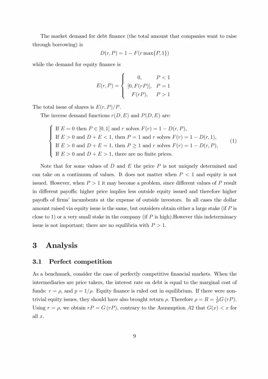
The market demand for debt �nance (the total amount that companies want to raise

through borrowing) is

D(r; P ) = 1� F (rmaxfP; 1g)

while the demand for equity �nance is

E(r; P ) =

8>><>>:0; P < 1

[0; F (rP )]; P = 1

F (rP ); P > 1

The total issue of shares is E(r; P )=P .

The inverse demand functions r(D;E) and P (D;E) are:8>>>><>>>>:If E = 0 then P 2 [0; 1] and r solves F (r) = 1�D(r; P ),If E > 0 and D + E < 1, then P = 1 and r solves F (r) = 1�D(r; 1),If E > 0 and D + E = 1, then P � 1 and r solves F (r) = 1�D(r; P ),If E > 0 and D + E > 1, there are no �nite prices.

(1)

Note that for some values of D and E the price P is not uniquely determined and

can take on a continuum of values. It does not matter when P < 1 and equity is not

issued. However, when P > 1 it may become a problem, since di¤erent values of P result

in di¤erent payo¤s; higher price implies less outside equity issued and therefore higher

payo¤s of �rms�incumbents at the expense of outside investors. In all cases the dollar

amount raised via equity issue is the same, but outsiders obtain either a large stake (if P is

close to 1) or a very small stake in the company (if P is high).However this indeterminacy

issue is not important; there are no equilibria with P > 1.

3 Analysis

3.1 Perfect competition

As a benchmark, consider the case of perfectly competitive �nancial markets. When the

intermediaries are price takers, the interest rate on debt is equal to the marginal cost of

funds: r = �, and p = 1=�. Equity �nance is ruled out in equilibrium. If there were non-

trivial equity issues, they should have also brought return �: Therefore � = R = 1PG (rP ).

Using r = �, we obtain rP = G (rP ), contrary to the Asuumption A2 that G(x) < x for

all x.

9

Thus, perfect competition implements the �rst best. All e¢ cient �rms (� � �) are�nanced, all ine¢ cient �rms are closed down. Equity is crowded out by debt because

equity �nancing involves a dilution cost due to asymmetric information. This is exactly

what a pecking order theory would imply in the absence of bankruptcy costs and costs of

�nancial distress. This result is also similar to Akerlof�s analysis of the lemons�problem.

In equilibrium with competitive intermediaries, equity should bring the same returns as

debt. But since only the best equity-�nanced �rms � = rP have returns equal to the

interest rate on debt, the average equity-�nanced �rm has quality below rP and is not

attractive to investors.

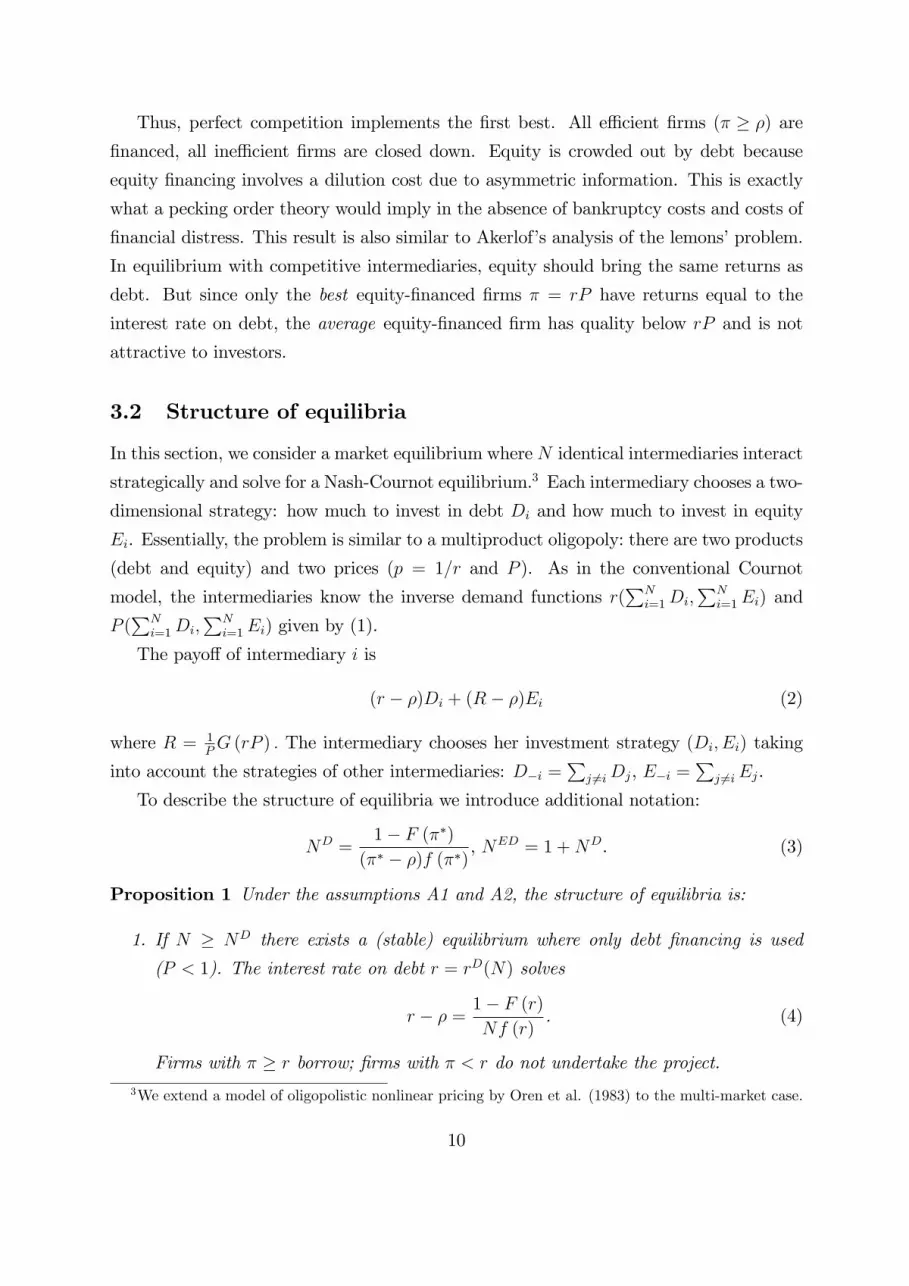
3.2 Structure of equilibria

In this section, we consider a market equilibrium where N identical intermediaries interact

strategically and solve for a Nash-Cournot equilibrium.3 Each intermediary chooses a two-

dimensional strategy: how much to invest in debt Di and how much to invest in equity

Ei. Essentially, the problem is similar to a multiproduct oligopoly: there are two products

(debt and equity) and two prices (p = 1=r and P ). As in the conventional Cournot

model, the intermediaries know the inverse demand functions r(PN

i=1Di;PN

i=1Ei) and

P (PN

i=1Di;PN

i=1Ei) given by (1).

The payo¤ of intermediary i is

(r � �)Di + (R� �)Ei (2)

where R = 1PG (rP ) : The intermediary chooses her investment strategy (Di; Ei) taking

into account the strategies of other intermediaries: D�i =P

j 6=iDj, E�i =P

j 6=iEj.

To describe the structure of equilibria we introduce additional notation:

ND =1� F (��)

(�� � �)f (��) , NED = 1 +ND. (3)

Proposition 1 Under the assumptions A1 and A2, the structure of equilibria is:

1. If N � ND there exists a (stable) equilibrium where only debt �nancing is used

(P < 1). The interest rate on debt r = rD(N) solves

r � � = 1� F (r)Nf (r)

. (4)

Firms with � � r borrow; �rms with � < r do not undertake the project.3We extend a model of oligopolistic nonlinear pricing by Oren et al. (1983) to the multi-market case.

10

2. If N � NED there exists a (stable) equilibrium where both debt and equity are used.

The price of equity is P = 1, the interest rate on debt solves

r �G(r) = 1� F (r)(N � 1) f (r) . (5)

Firms with � � r borrow, �rms with � < r issue equity.

3. If N 2�ND; NED

�there exists an (unstable) equilibrium where both equity and debt

are used. The price of equity is P = 1, the interest rate on debt is r = ��. Firms

with � � r borrow, �rms with � < r use equity or do not undertake the project.

The comparative statics of equilibria with respect to market structure N is illustrated

in Figure 2. If the �nancial markets are perfectly competitive, N ! 1, then equity iscompletely crowded out by debt and there exists a unique equilibrium which approxi-

mates the �rst best, rD(N) ! �. If the �nancial markets are highly concentrated, then

there exists a unique equilibrium in which all �rms are �nanced: good �rms borrow and

bad �rms issue equity.4 In the intermediate range of concentration, there are multiple

equilibria.

The intuition behind the structure of equilibria is quite straightforward. First, be-

cause �nancial markets are imperfectly competitive, the interest rate on debt is set above

investors�cost of funds and the markup, r� �, decreases with N . Secondly, at every levelof concentration, N , the interest rate on debt in equilibrium with both equity and debt is

higher than in equilibrium with debt only. The incentives to raise interest rates (through

reduced lending) in an equilibrium without equity are lower; by increasing interest rates

the intermediaries earn higher returns from borrowers but lose clients. In an equilibrium

with both debt and equity higher interest rates generate higher returns on borrowers.

The �rms which stop borrowing do not drop out but switch to equity �nance and bring

additional pro�ts to the intermediaries. Third, an equilibrium with equity exists if and

only if the interest rate on debt is su¢ ciently high, r � ��, so that the average quality ofequity-�nanced �rms is also high, G(r) � G(��) = �, while an equilibrium without equityrequires the opposite, r � ��.Multiple equilibria emerge as a result of the strategic complementarities generated

by the return-on-equity externality. When an intermediary decides to lend more, the

4This result is consistent with Petersen and Rajan (1995) who show that a monopoly lender is more

likely to form a relationship with the �rm e¤ectively obtaining a stake in �rm�s future pro�ts, similar to

equity �nancing in our model.

11

r

0NED

π*

Equilibria with debt and equity

Equilibria with debt

ND N

ρ

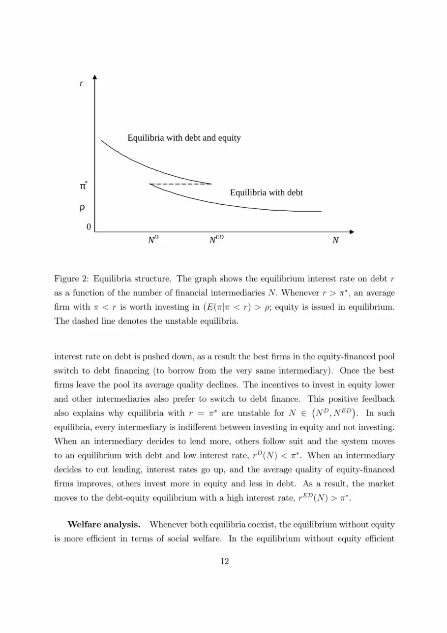
Figure 2: Equilibria structure. The graph shows the equilibrium interest rate on debt r

as a function of the number of �nancial intermediaries N: Whenever r > ��; an average

�rm with � < r is worth investing in (E(�j� < r) > �; equity is issued in equilibrium.

The dashed line denotes the unstable equilibria.

interest rate on debt is pushed down, as a result the best �rms in the equity-�nanced pool

switch to debt �nancing (to borrow from the very same intermediary). Once the best

�rms leave the pool its average quality declines. The incentives to invest in equity lower

and other intermediaries also prefer to switch to debt �nance. This positive feedback

also explains why equilibria with r = �� are unstable for N 2�ND; NED

�. In such

equilibria, every intermediary is indi¤erent between investing in equity and not investing.

When an intermediary decides to lend more, others follow suit and the system moves

to an equilibrium with debt and low interest rate, rD(N) < ��. When an intermediary

decides to cut lending, interest rates go up, and the average quality of equity-�nanced

�rms improves, others invest more in equity and less in debt. As a result, the market

moves to the debt-equity equilibrium with a high interest rate, rED(N) > ��.

Welfare analysis. Whenever both equilibria coexist, the equilibrium without equity

is more e¢ cient in terms of social welfare. In the equilibrium without equity e¢ cient

12

�rms with � 2 (�; rD(N)) are not �nanced resulting in the deadweight loss ofR rD(N)�

(���)f(�)d�. In the equilibrium with equity, intermediaries cannot discriminate among �rms

within the equity pool, � 2 [0; rED(N)]. As a result, ine¢ cient �rms � 2 [0; �) are also�nanced resulting in the deadweight loss of

R ��(� � �)f(�)d�. The equilibrium without

equity is less ine¢ cient when the average �rm that is denied �nancing should not have

been �nanced in the �rst best: G(rD(N)) < �: This condition is equivalent to rD(N) < ��

which follows from the existence of the equilibrium without equity.

Certainly, the welfare results should not be interpreted literally as a call to outlaw

equity �nancing. First, we assume away all the costs of debt. Second, it is very likely

that due to imperfections in the primary markets for funds for the banks, their costs of

funds � is above social cost of funds. Therefore when equity �nance helps to implement

projects with returns below �, it may actually be socially optimal.

Example. Consider f(�) = 1=(� � �) for � 2 [�; �]: Uniform distribution satis�es

both assumptions A1 and A2, so there can be at most two stable equilibria: one with

debt, and the other one with debt and equity. Indeed, G(�) = (� + �)=2; �� = 2� � �;NED = (� � �)=(� � �); ND = NED � 1. The equilibrium with debt �nancing exists

whenever N � ND: In this equilibrium the interest rate is rD(N) = (N� + �)=(N + 1);

the deadweight loss is (���)2= [2(N + 1)2(� � �)] : The equilibrium with debt and equity�nancing exists wheneverN � NED; the interest rate is rED(N) = ((N�1)�+2�)=(N+1);the deadweight loss is (�� �)2= [2(� � �)].

Monopoly. We do not consider the special case of monopolistic intermediary. It is

formally equivalent to the solution above at N = 1: The only di¤erence is that there are

no multiple equilibria: the monopolist chooses the one which is best for him. If E� > �;

the monopolistic equilibrium is one with equity P = 1; r = �; actually there is no debt

in this equilibrium. If E� < � < �; there is debt and no equity: P < 1; r = rD(1).

Cournot vs Bertrand competition. We have assumed above that the intermedi-

aries compete a la Cournot. One could also rede�ne our model as Bertrand competition

in a two-stage framework along the lines of Kreps and Scheinkman (1983). Suppose that

the �nancial intermediaries �rst have to precommit capacities (mostly human capital)

for delivering services in debt and equity markets; in the second stage the compete a la

Bertrand in stock and debt prices. This setup would be equivalent to our model; the

choice of capacities is exactly the choice of Di and Ei: In the �rst stage, the intermedi-

13

r

  (1­F(r))/f(r)   (N­1)(r­G(r))

Figure 3: Multiple equilibria with equity. The thick line depicts the left-hand side of (5);

the thin line is the right-hand side.

aries may set Di and Ei as high as they wish, but in the second stage, they cannot go

beyond these pre-committed capacities (or they can only at a marginal cost of resources

being much higher than �). In the Section 4.1 we study a model of Bertrand competition

with di¤erentiated goods which produces similar results even though being much more

complex.

3.3 An example: Multiple equilibria with equity

This Section provides an example illustrating that once the assumptions A1 and A2 are

relaxed, there can exist multiple equilibria of each type. In particular, it shows that there

can be two equilibria with equity which di¤er in terms of both stock returns and amounts

of equity �nancing.

Suppose that � is distributed on [�; �] with the density function:

f(�) =

8>>>><>>>>:0:6=(� � �), if � � � < 0:75� + 0:25�

1:4=(� � �), if 0:75� + 0:25� � � < 0:5� + 0:5�

0:6=(� � �), if 0:5� + 0:5� � � < 0:25� + 0:75�

1:4=(� � �), if 0:25� + 0:75� � � � �

which does not satisfy the monotone hazard ratio property (see Figure 3).

14

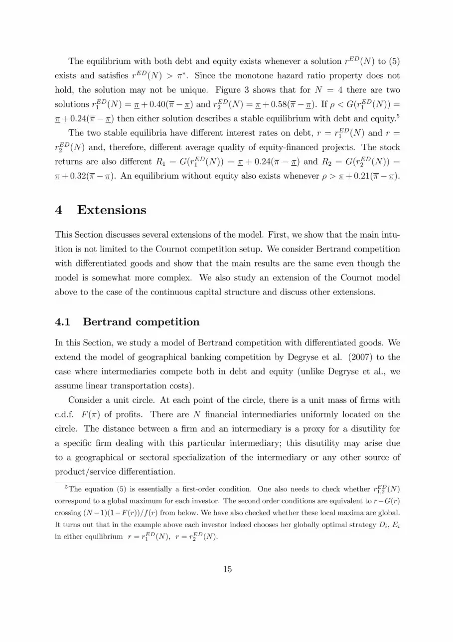
The equilibrium with both debt and equity exists whenever a solution rED(N) to (5)

exists and satis�es rED(N) > ��. Since the monotone hazard ratio property does not

hold, the solution may not be unique. Figure 3 shows that for N = 4 there are two

solutions rED1 (N) = �+0:40(�� �) and rED2 (N) = �+0:58(�� �). If � < G(rED1 (N)) =

�+0:24(�� �) then either solution describes a stable equilibrium with debt and equity.5

The two stable equilibria have di¤erent interest rates on debt, r = rED1 (N) and r =

rED2 (N) and, therefore, di¤erent average quality of equity-�nanced projects. The stock

returns are also di¤erent R1 = G(rED1 (N)) = � + 0:24(� � �) and R2 = G(rED2 (N)) =

�+0:32(�� �). An equilibrium without equity also exists whenever � > �+0:21(�� �).

4 Extensions

This Section discusses several extensions of the model. First, we show that the main intu-

ition is not limited to the Cournot competition setup. We consider Bertrand competition

with di¤erentiated goods and show that the main results are the same even though the

model is somewhat more complex. We also study an extension of the Cournot model

above to the case of the continuous capital structure and discuss other extensions.

4.1 Bertrand competition

In this Section, we study a model of Bertrand competition with di¤erentiated goods. We

extend the model of geographical banking competition by Degryse et al. (2007) to the

case where intermediaries compete both in debt and equity (unlike Degryse et al., we

assume linear transportation costs).

Consider a unit circle. At each point of the circle, there is a unit mass of �rms with

c.d.f. F (�) of pro�ts. There are N �nancial intermediaries uniformly located on the

circle. The distance between a �rm and an intermediary is a proxy for a disutility for

a speci�c �rm dealing with this particular intermediary; this disutility may arise due

to a geographical or sectoral specialization of the intermediary or any other source of

product/service di¤erentiation.

5The equation (5) is essentially a �rst-order condition. One also needs to check whether rED1;2 (N)

correspond to a global maximum for each investor. The second order conditions are equivalent to r�G(r)crossing (N�1)(1�F (r))=f(r) from below. We have also checked whether these local maxima are global.It turns out that in the example above each investor indeed chooses her globally optimal strategy Di; Eiin either equilibrium r = rED1 (N), r = rED2 (N):

15

The intermediaries face a cost of funds � and provide funding to the �rms either

through debt or through equity. Each intermediary i sets the interest on the debt ri and

the price of equity Pi. Each �rm then decides whether to undertake a project or not,

whether to �nance it via debt or equity, and which intermediary to choose: each �rm

solves maxi=1;:::;N maxf�� ri � �xi; �� �=Pi � �xi; 0g where � is the �rm�s returns, xi isthe distance to intermediary i; and � is the transportation cost per unit of distance.

The aggregate demand for debt and equity �nancing is therefore a function of prices

ri and Pi set by all the intermediaries. We will solve for a Nash equilibrium where each

intermediary chooses ri and Pi to maximize her pro�ts given the strategies r�i and P�iof all the other intermediaries.

We will only consider symmetric equilibria where all the intermediaries end up with

the same strategies ri = r�i and Pi = P�i. In these equilibria, all intermediaries compete

only with their neighbors on the circle. Therefore, instead of studying the circle, we can

limit our analysis to that of price competition on an interval of length 1=N .

The structure of equilibria depends on the intensity of competition (proxied by the

number of intermediaries N). In the case of perfect competition (N ! 1); the interestrate is set at ri = �; and there is no equity issue. If competition is strong (1=N is small)

then there are equilibria where �rms issue debt but not equity �the intermediaries know

that the equity issuing �rms are on average only worth �nancing at stock price below 1;

but at these prices �rms prefer not to issue equity at all. These equilibria are depicted in

the Figure 4a)

If the competition is su¢ ciently weak (1=N is large) then the equilibrium involves

equity issues. Similarly to the Cournot model above, the interest rate on debt is so

high, that the average �rm that cannot a¤ord issuing debt at these rates is su¢ ciently

pro�table. Hence, a stock price Pi � 1 pays o¤ for the intermediary. There are two typesof such equilibria: in the case shown in the Figure 4b, intermediaries competes between

each other only for the better �rms (which are �nanced via debt); this equilibrium takes

place if riPi = �=(2N) + ri: Figure 4c presents the other case where the intermediaries

compete both for the debt-issuing �rms and for the equity-issuing �rms.

In the Appendix B, we solve for the equilibria and show that the main results are

similar to those obtained in the Cournot model above. In particular, interest rate on

debt increases with market concentration 1=N ; in turn, the higher the interest rate, the

more valuable the equity-issued �rms are which in turn results in broader equity markets

(i.e. number of equity issuing �rms increases in 1=N). The important di¤erence from the

16

D1

π

x1/N0

E2E1

r1P1

D2

(c) Debt and equity

D1 D2

(b) Debt and equity

x

π

E1

1/N0

E2r1P1

D1 D2

(a) Debt only

x

π

1/N0

r1

Figure 4: Equilibria in Bertrand competition with di¤erentiated goods. (a) is the equi-

librium where only debt is issued. (b) and (c) are the equilibria where �rms issue debt

and equity. Areas Di and Ei denote �rms �nanced through intermediary i via debt and

equity, respectively. Other �rms do not invest.

Cournot setting is that the price of equity is above 1 (so that most equity issuers do earn

positive rents).

Figure 5 shows the equilibrium interest rate on debt as a function of number of inter-

mediaries N in the case where F (�) is a uniform distribution. The structure of equilibria

is much like the one in the Cournot model (see Fig. 2). First, equilibria with debt and

equity exist as long as market is su¢ ciently concentrated (in this example, N � 10). Sec-ond, equilibria with debt only �nancing exist if market is su¢ ciently competition (N � 5):Third, there is a range of market structures (in this example, for N 2 [5; 10]) when thetwo equilibria co-exist.

4.2 Continuous choice of capital structure.

The model above allowed only a binary choice of capital structure: either debt or equity.

If the �rms can choose any combination of debt and equity, capital structure provides

intermediaries with a more informative signal of the �rm�s type. As better �rms use

more debt, intermediaries will price higher the stock of �rms with lesser reliance on

outside equity. Yet, the strategic complementarity discussed above is still present. If one

17

0

1

2

3

4

0 2 4 6 8 10 12

N

r

Equilibria with debt and equity

Equilibria with debt

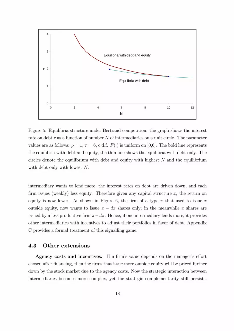
Figure 5: Equilibria structure under Bertrand competition: the graph shows the interest

rate on debt r as a function of number N of intermediaries on a unit circle. The parameter

values are as follows: � = 1; � = 6; c.d.f. F (�) is uniform on [0,6]. The bold line representsthe equilibria with debt and equity, the thin line shows the equilibria with debt only. The

circles denote the equilibrium with debt and equity with highest N and the equilibrium

with debt only with lowest N:

intermediary wants to lend more, the interest rates on debt are driven down, and each

�rm issues (weakly) less equity. Therefore given any capital structure x, the return on

equity is now lower. As shown in Figure 6, the �rm of a type � that used to issue x

outside equity, now wants to issue x � dx shares only; in the meanwhile x shares areissued by a less productive �rm ��d�. Hence, if one intermediary lends more, it providesother intermediaries with incentives to adjust their portfolios in favor of debt. Appendix

C provides a formal treatment of this signalling game.

4.3 Other extensions

Agency costs and incentives. If a �rm�s value depends on the manager�s e¤ort

chosen after �nancing, then the �rms that issue more outside equity will be priced further

down by the stock market due to the agency costs. Now the strategic interaction between

intermediaries becomes more complex, yet the strategic complementarity still persists.

18

Firm’stype π

π_π

Outsideequity1­α

Figure 6: Strategic complementarity in a setting with continuous choice of capital struc-

ture. In any equilibrium, better �rms issue (weakly) more debt. As interest rate goes

down, each �rm reduces its reliance on equity �nance. Therefore, for any given capi-

tal structure �; investors expect a lower type � and therefore lower returns to equity

investment.

As one intermediary purchases less debt, an increased interest rate drives marginal �rms

from debt to equity �nancing. While the value of the marginal �rm is negatively a¤ected

by the agency costs, the average quality of equity �nanced project improves. Thus other

intermediaries also move away from debt. In Appendix C we formally introduce agency

costs in our model.

Costs of �nancial distress. For simplicity, we have assumed away costs of debt

�nancing. If the project returns � are stochastic, and the �rm faces either the incentive

e¤ects of debt overhang, or costs of �nancial distress and ine¢ cient litigation, or costs

of intermediated bank lending (as in Bolton and Freixas, 2000), in any equilibrium some

�rms will use both debt and equity. Yet, as the structure of sorting does not change

(better �rms prefer more debt), the main result will remain intact.

Positive payo¤ to equity issuers. The fact that the equity issuing �rms obtain

trivial payo¤ and are indi¤erent between issuing equity and shutting down is an artefact

of the simple setup. As shown above, this issue disappears once we move away from

Cournot to Bertrand oligopoly. One could also consider a Cournot model with an outside

19

option: suppose that if the �rm does not invest, its owner-manager can earn a reservation

utility � > 0: Then the equilibrium with equity would involve the payo¤ of � to the �rm.

The capital structure choice would be as follows. If P < 1 + �=r then there is no equity

�nancing: good �rms (� > r+�) borrow, others do not invest. If P > 1+�=r, the choice

is even richer: best �rms (� > rP ) borrow, intermediate �rms (� 2 (�P=(P � 1); rP ))issue equity, the least pro�table �rms (� < �P=(P � 1)) do not invest. Therefore themarket demand for debt is D = 1 � F (maxfr + �; rPg); and the market demand forequity is F (rP ) � F (�P=(P � 1)) if P > 1 + �=r and zero otherwise. These functionshave the same features that drive our results: (i) the better �rms issue debt rather than

equity, and (ii) the higher the interest rate on debt, the more �rms switch from debt to

equity.

Observed heterogeneity. The pecking-order theory intuition that equity is subop-

timal to debt predicts that better and safer �rms use debt while �rms that are denied debt

�nancing or those that have already borrowed too much, resort to equity. In real world,

there are other factors that determine the choice of capital structure. Given that equity

�nance involves a �xed cost of issue, larger �rms are more likely to opt for stock market.

At the same time, the larger �rms may also have safer returns, so the sign of correlation

between capital structure and source of funding may change. Still, our model would be

relevant suggesting that among the �rms with the same observed characteristics (such as

size or sector), the ones that prefer debt are probably the ones with better prospects (this

is consistent with empirical evidence surveyed in Myers, 2000).

5 Conclusions

This paper studies a model of imperfect competition in �nancial markets with endogenous

capital structure. The model builds on the pecking order theory that assumes that �rms

are better informed about their growth opportunities than outside investors. An issue

of equity sends investors a negative signal about the �rm�s quality; the cost of equity

�nancing is always higher than that of debt �nance. Therefore, in the absence of the

costs of �nancial distress the �rms should �nance their investment via internal funds or

debt. Such conclusion, however, hinges on the assumption that �nancial markets are

perfectly competitive, so that all the imperfections of equity �nance are automatically

passed back to the �rm in the form of a higher cost of capital.

20

We show that when �nancial markets are concentrated, this does not have to be the

case: returns on equity and debt may di¤er. In the presence of oligopoly in �nancial

markets, some �rms issue equity even if there are no costs associated with debt �nancing.

The intuition is straightforward: oligopolistic �nancial intermediaries set interest rate

on debt above their cost of funds. Hence, there are �rms that would be �nanced in

perfectly-competitive economy but who cannot a¤ord to borrow under oligopoly. The

intermediaries are happy to �nance these �rms but do not like to lower interest rates

for their more pro�table debtors. Capital structure emerges as an e¤ective tool for the

(second degree) price discrimination: the most pro�table �rms prefer to be �nanced via

debt rather than switch to equity.

An important implication of our analysis is the multiplicity of equilibria due to strate-

gic interaction between oligopolistic �nancial intermediaries. The intermediaries�portfolio

choices are strategic complements: if one intermediary moves from debt- to equity-holding,

others �nd it pro�table to follow. When a large intermediary reduces lending and invests

more in equity, interest rate on debt goes up. Hence, some �rms that used to be �nanced

via debt have to switch to equity �nancing. As the marginal equity-�nanced �rms are al-

ways better than the average equity-�nanced �rms, this improves the expected returns on

equity. Therefore investing in equity becomes relatively more attractive to other investors

as well. The strategic complementarity results in multiplicity of equilibria. The latter

in turn may explain the volatility of stock returns, and stock market crashes. Strictly

speaking, there are no bubbles in the model: investors price each stock based on the

rationally updated expectations of this stock�s returns. However, the returns are endoge-

nous and are not uniquely determined given the multiplicity of equilibria. Our model

suggest that stock crashes can occur even if there are no bubbles. Certainly, in order to

fully explore the stock price dynamics, one has to build a multi-period setup which is an

exciting avenue for further research.

While we develop implications for the volatility in a public stock market, our model

if taken literally is a model of an entrepreneur raising capital for a new project. While

our intuition is not constrained to this case, a few formal extensions are due to make the

argument more convincing: �rst, consider the case with existing assets, second, consider

secondary markets for stocks, third, introduce a con�ict between management and initial

shareholders (Dybvig and Zender, 1993, showed the implications of the latter for the

validity of the pecking order theory).

21

Appendix A: Proofs

Proof of Proposition 1.

Equilibria without equity.

Suppose that the equilibrium price of equity is low, P < 1. Then, no equity is issued

and the equilibrium is a standard equilibrium of a single-product oligopoly. The inverse

demand function implies dr=dDi = �1=f(r). The �rst order condition for intermediary iis

(r � �)�Di=f(r) = 0

Summing up across investors i = 1; :::; N and dividing by N , we obtain (4). A1 implies

that the right-hand side of (4) decreases in r, hence there exists a unique solution denoted

by rd(N). Clearly, rd(N) decreases with N and as N ! 1, the solution approaches theperfectly competitive one, rd(N)! �.

This equilibrium exists whenever no intermediary could bene�t from equity invest-

ment. Hence, Ei must be an optimal strategy for every i. This is the case whenever

the average quality of stock of �rms that are not issuing debt is below the marginal cost

of funds R = G(r) � �: Thus, the equilibrium exists whenever rd(N) � �� which is

equivalent to N � ND:

Equilibria with equity.

Suppose that P � 1; so �rms with � � rP may issue equity. First, we will show thatP > 1 cannot hold in equilibrium. Suppose that there is an equilibrium with P = eP > 1,and r = er: Then the following conditions should hold: (i) PN

i=1Di +PN

i=1Ei = 1;

(ii)PN

i=1Di = 1 � F (rP ); (iii) there is an intermediary i who holds non-trivial equityposition Ei > 0:We will argue that this intermediary will always have incentives to reduce

her investment in equity. Even a small decrease in equity investment results in a discrete

drop in stock price from eP to 1: Since the supply of debt fundingPNi=1Di does not change,

the interest rate on debt will adjust accordingly to r = er eP so that Di+D�i = 1�F�er eP�

remains the same. Then the intermediary i�s payo¤will increase: the �rst term in (2) will

not change, while the second one will certainly increase: the decline in Ei is in�nitesimal,

while R jumps from G�er eP� = eP to G

�er eP� : Therefore equilibria with equity can onlyexist under P = 1:

There can be two types of equilibria P = 1: with full investmentPN

i=1Di+PN

i=1Ei =

1 and rationed investmentPN

i=1Di+PN

i=1Ei < 1. Let us �rst consider the equilibria with

full investment. Then intermediary i maximizes rDi+G (r)Ei: The �rst-order condition

22

is

0 = r �G(r)� 1

f(r)(Di +G

0(r)Ei)

Summing up and using G0(x) = (x�G(x))f(x)=F (x) we obtain (5). Under the assump-tions A1 and A2, the left-hand side increases in r while the right-hand side decreases in

r. Hence the solution rED(N) is unique and (as it is easy to show) decreases in N:

Full investment Di+Ei = 1� (D�i + E�i) is an equilibrium strategy if and only if the

maximum investment in equity is optimal. In other words, the return on equity should

be above the cost of funds: R = G(rED(N)) � �. In other words, rED(N) � �� which isequivalent to N � NED.

The last type of equilibria is the one with debt and equity where some �rms do not

undertake the project. This occurs when P = 1 but Di + Ei < 1 � (D�i + E�i). The

investors are indi¤erent about buying more equity. This may happen only if G(r) = �; or

r = ��: In this equilibrium, the �rst order condition for Di is as follows:

(r � �)� 1

f(r)(Di +G

0(r)Ei) = 0

Adding up for i = 1; :::; N we obtain

N(r � �)� 1� F (r)f(r)

� (r �G(r))PN

i=1EiF (r)

= 0

After substituting r = ��

NXi=1

Ei=F (��) = N � 1

r � �1� F (r)f(r)

The equilibrium exists whenever 0 <PN

i=1Ei < F (��): One can easily check that the left

inequality is equivalent to N > ND; while the right inequality is equivalent to condition

is equivalent to N < NED:

Appendix B: Bertrand competition

In this Appendix, we will describe the equilibria in Figure 4 and fully solve an example

with uniform distribution F (�) on [0; �] (assuming that � is su¢ ciently high).

Let us denote the transportation costs between two neighboring intermediaries � =

�=N and from now one measure the distances in terms of respective transportation costs.

23

Equilibria without equity. First, we will consider equilibria without equity (Fig.4a).

The condition for these equilibria to exist is to make sure that ri is su¢ ciently low in equi-

librium so even for the �rms with xi = 0 there is no equity issue in equilibrium even at

share price Pi = 1: This condition impliesR ri0(� � �)f(�)d� < 0:

Let us describe the intermediary 1�s optimization problem. Given the interest rate of

its neighbor r2; the �rst intermediary solve

maxri

Z �+r2�r12

0

(r1 � �)(1� F (r1 + x))dx

Di¤erentiating this equation with regard to r1 and then using the symmetric equilibrium

condition r1 = r2 = r; we �nd the following equation for the equilibrium interest rate:

0 =

Z �2

0

(1� F (r + x))dx� 12(r � �)

�1� F

�r +

�

2

��� (r � �)F

��

2

�Equilibrium with debt and equity Let�s �rst start with the case where interme-

diaries compete in debt markets only (Fig.4b). This is the case whenever

r1(P1 � 1) <1

2(� + r2 � r1) (6)

where r2 is the interest rate set by the competitor 2 and r1; P1 are the choice of the

intermediary 1.

The �rst intermediary�s total payo¤ is

U =

Z r1P1

0

��

P1� �

��(P1 � 1)

P1f(�)d� + (r1 � �)

Z �+r2+r12

r1P1

(� � r1)f(�)d� +

+(r1 � �)Z 1

�+r2+r12

�+ r2 � r12

f(�)d�

The f.o.c.s with regard to r and P are as follows

0 = Ur =

Z �+r2+r12

r1P1

f(�)d�(� � r1) +Z 1

�+r2+r12

f(�)d��+ r2 � r1

2� (7)

� (r1 � �)�1

2+1

2F

��+ r2 + r1

2

�� F (r1P1)

�

0 = UP =�1P 2

Z rP

0

�f(�)d�h� + �� 2 �

P

iAs the equilibrium is symmetric ri = r; Pi = P , these equations become

24

∆/2

C

B

A

Debt 1

r1P1

Equity 2

∆

x=π(P1­1)/P1

Debt 2

Equity 1

π

x

x=∆­π(P2­1)/P2

x=(∆+r2­r1)/2

r2P2

x=(∆+r2­π/P1)/2

x=(∆+π/P2­π/P1)/2

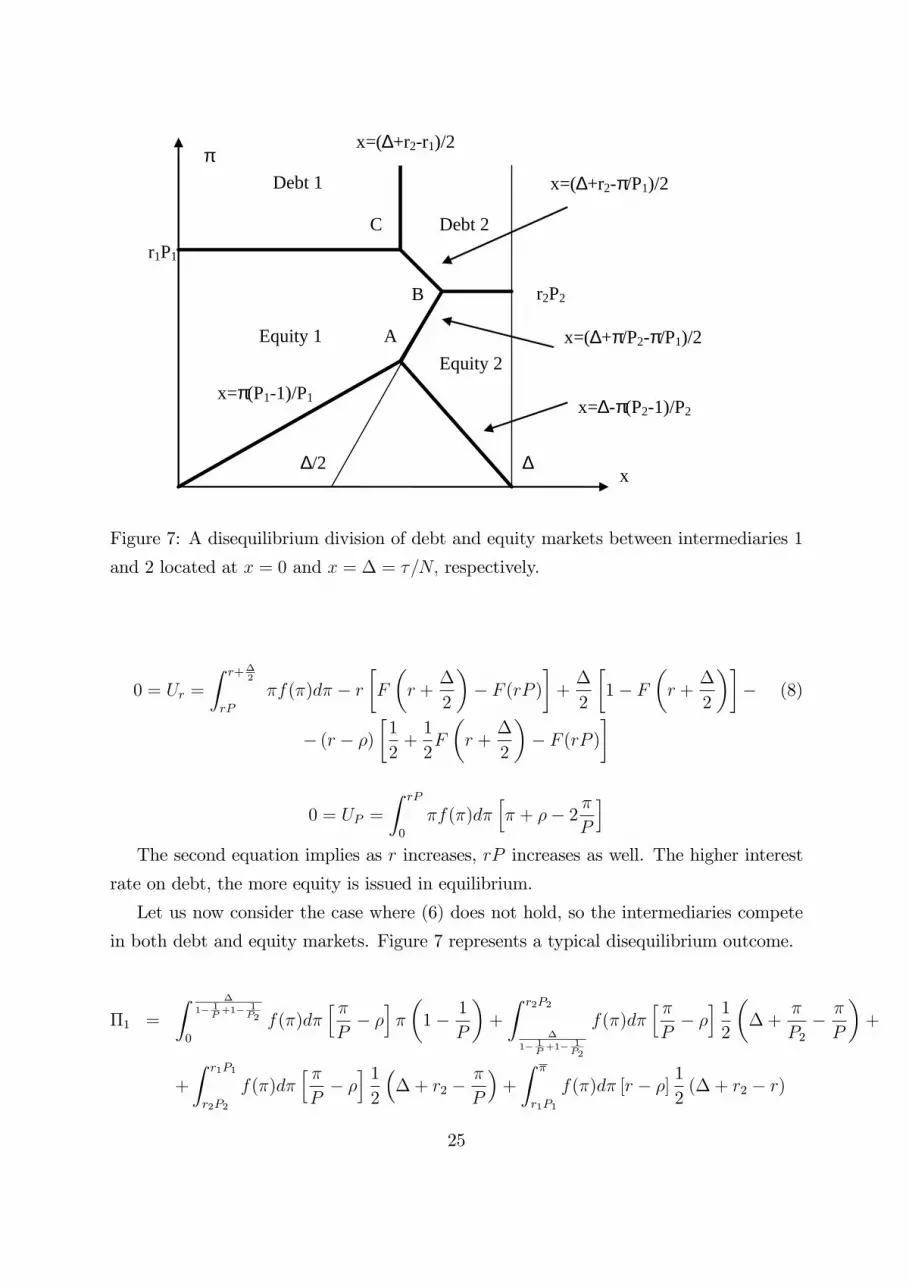
Figure 7: A disequilibrium division of debt and equity markets between intermediaries 1

and 2 located at x = 0 and x = � = �=N; respectively.

0 = Ur =

Z r+�2

rP

�f(�)d� � r�F

�r +

�

2

�� F (rP )

�+�

2

�1� F

�r +

�

2

��� (8)

� (r � �)�1

2+1

2F

�r +

�

2

�� F (rP )

�

0 = UP =

Z rP

0

�f(�)d�h� + �� 2 �

P

iThe second equation implies as r increases, rP increases as well. The higher interest

rate on debt, the more equity is issued in equilibrium.

Let us now consider the case where (6) does not hold, so the intermediaries compete

in both debt and equity markets. Figure 7 represents a typical disequilibrium outcome.

�1 =

Z �

1� 1P+1� 1

P2

0

f(�)d�h �P� �

i�

�1� 1

P

�+

Z r2P2

�

1� 1P+1� 1

P2

f(�)d�h �P� �

i 12

��+

�

P2� �

P

�+

+

Z r1P1

r2P2

f(�)d�h �P� �

i 12

��+ r2 �

�

P

�+

Z �

r1P1

f(�)d� [r � �] 12(� + r2 � r)

25

Let us �nd the �rst order conditions:

@U

@r=1

2[1� F (rP )] (r � �) (� + r2 � r) :

Hence the r1 = 12(� + �+ r2) : In the symmetric equilibrium r1;2 = �+�:

Let us now �nd the derivative with regard to the stock price:

@U

@ (1=P1)=

Z �

1� 1P+1� 1

P2

0

�f(�)d�

�� + �� 2 �

P1

�+1

2

Z r2P2

�

1� 1P+1� 1

P2

�f(�)d�

��+ �+

�

P2� 2 �

P1

�+

+1

2

Z r1P1

r2P2

f(�)d�

��+ �+ r2 � 2

�

P1

�:

As we solve for the symmetric equilibrium, this becomes

0 =

Z �P2(P�1)

0

�f(�)d�h� + �� 2 �

P

i+1

2

Z (�+�)P

�P2(P�1)

�f(�)d�h�+ �� �

P

i

Uniform distribution. A straightforward substitution of F (�) = �=� into the

equation above results in two quadratic equations and one cubic equation. Solving those

we obtain Fig. 5. Finally, it is easy to show that in the uniform case, the equilibria with

debt and equity exist whenever r > 32� while the equilibria with debt only exist whenever

r < 2�:

Appendix C: Continuous choice of capital structure

In this section, we add two ingredients to the model: we introduce agency costs and allow

for any combinations of debt and equity. We set up the model, introduce the equilibrium

concept, and show that there is a strategic complementarity similar to the one in the main

model. As one intermediary buys more debt, the interest rate goes down, better �rms

switch to debt. Hence quality of equity goes down, and other investors have incentives to

sell equity and buy debt.

Production technology. The �rm�s pro�t � is uncertain; its distribution depends

on the manager�s e¤ort. There are two outcomes: �low�� = �L > 0 and �high�� = �H =

�L+�; where � > 0: The manager�s e¤ort is measured in terms of probability of achieving

the high outcome.

26

The cost of e¤ort depends on the manager�s type �; the cost is �C(e; �); where Ce �0; Ce(0; �) = 0; Cee > 0; C� < 0; Ce� < 0: The type (productivity) � is distributed on

[0;1] with c.d.f. F (�):We assume an internal maximum; in other words, the parametersare such that even the �rst best choice of e¤ort (probability e that solves Ce(e; �) = 1) is

in [0; 1] for all �.

Financial contracts. The �rm needs to raise one unit of capital via issuing debt,

equity or a combination of the two. Given the price of debt p = 1=r (dollars raised per

dollar to be repaid) and price of equity is P (in dollars per 100 percent of cash �ows), the

�rm borrows D � 0 and issues 1� � shares. The budget constraint is as follows:

(1� �)P +D � 1: (9)

Given the pro�t is �i; i = L;H, the �rm pays rD to creditors and (1 � �)(�i � rD) tooutside shareholders keeping �(�i � rD) for itself.In what follows we assume that r < �L in equilibrium so there are no bankruptcies.

Under limited liability we only need to consider contracts with D � �L: Any contract

with � 2 [0; 1] and D > �L can be replicated by a contract with eD = �L and e� =���1

��H �D

�+:

E¤ort choice. The �rm maximizes

� = �(�L � rD)(1� e) + �(�H � rD)e� �C(e; �) = ��L � �rD + v(�; �)� (10)

where

v(�; �) = maxe2[0;1]

[�e� C(e; �)]

Using the envelope theorem (or monotone comparative statics), one can easily prove that

v� � 0; v� � 0; v�� � 0; v�� � 0 (the single crossing property holds).6 We denote e�(�; �)the solution to � = C(e; �): The e¤ort level e�(�; �) = v�(�; �) (weakly) increases both in

type � and in the share of equity � kept by the manager.

If the �rm does not undertake the project, the manager gets her reservation value u.

Since incentives depend on the capital structure �, the investors will certainly expect

lower returns on equity of �rms with higher outside equity 1 � �: Therefore, the stockprice P should depend on the capital structure � as well. Since there are no bankruptcies,

the rate of return on debt will be the same for all �rms (a dollar invested in debt always

brings r dollars whoever the borrower is).

6If C(e; �) = e2=(2�) then v(�; �) = ��2=2:

27

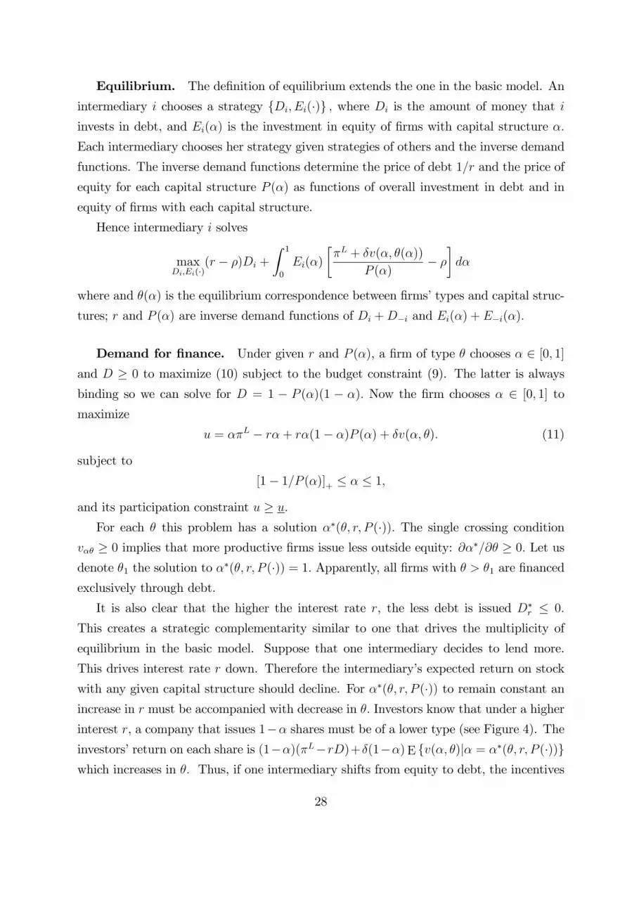
Equilibrium. The de�nition of equilibrium extends the one in the basic model. An

intermediary i chooses a strategy fDi; Ei(�)g ; where Di is the amount of money that i

invests in debt, and Ei(�) is the investment in equity of �rms with capital structure �:

Each intermediary chooses her strategy given strategies of others and the inverse demand

functions. The inverse demand functions determine the price of debt 1=r and the price of

equity for each capital structure P (�) as functions of overall investment in debt and in

equity of �rms with each capital structure.

Hence intermediary i solves

maxDi;Ei(�)

(r � �)Di +

Z 1

0

Ei(�)

��L + �v(�; �(�))

P (�)� �

�d�

where and �(�) is the equilibrium correspondence between �rms�types and capital struc-

tures; r and P (�) are inverse demand functions of Di +D�i and Ei(�) + E�i(�):

Demand for �nance. Under given r and P (�), a �rm of type � chooses � 2 [0; 1]and D � 0 to maximize (10) subject to the budget constraint (9). The latter is always

binding so we can solve for D = 1 � P (�)(1 � �): Now the �rm chooses � 2 [0; 1] tomaximize

u = ��L � r� + r�(1� �)P (�) + �v(�; �): (11)

subject to

[1� 1=P (�)]+ � � � 1;

and its participation constraint u � u:For each � this problem has a solution ��(�; r; P (�)): The single crossing condition

v�� � 0 implies that more productive �rms issue less outside equity: @��=@� � 0: Let usdenote �1 the solution to ��(�; r; P (�)) = 1: Apparently, all �rms with � > �1 are �nancedexclusively through debt.

It is also clear that the higher the interest rate r, the less debt is issued D�r � 0:

This creates a strategic complementarity similar to one that drives the multiplicity of

equilibrium in the basic model. Suppose that one intermediary decides to lend more.

This drives interest rate r down. Therefore the intermediary�s expected return on stock

with any given capital structure should decline. For ��(�; r; P (�)) to remain constant anincrease in r must be accompanied with decrease in �: Investors know that under a higher

interest r, a company that issues 1�� shares must be of a lower type (see Figure 4). Theinvestors�return on each share is (1��)(�L�rD)+�(1��) E fv(�; �)j� = ��(�; r; P (�))gwhich increases in �: Thus, if one intermediary shifts from equity to debt, the incentives

28

of others to invest in equity may also decline. Yet, unlike in the model of the previous

section, we also need to check for change in stock price P (�) in response to lower interest

rate. This is what is done below.

Solving for inverse demand functions. We will �nd r and P (�)�price of debt

and price of stock of �rm with capital structure ��given total amount borrowed D =PiDi and total funds raised via issues of equity by �rms with the same capital structure

E(�) =P

iEi(�) � 0 (we naturally assume E(1) = 0). We will also solve for the (weaklymonotonic) correspondence between �rm�s type and capital structure �(�):

First, we can �nd the lowest type that is �nanced �. By de�nition, this type has capital

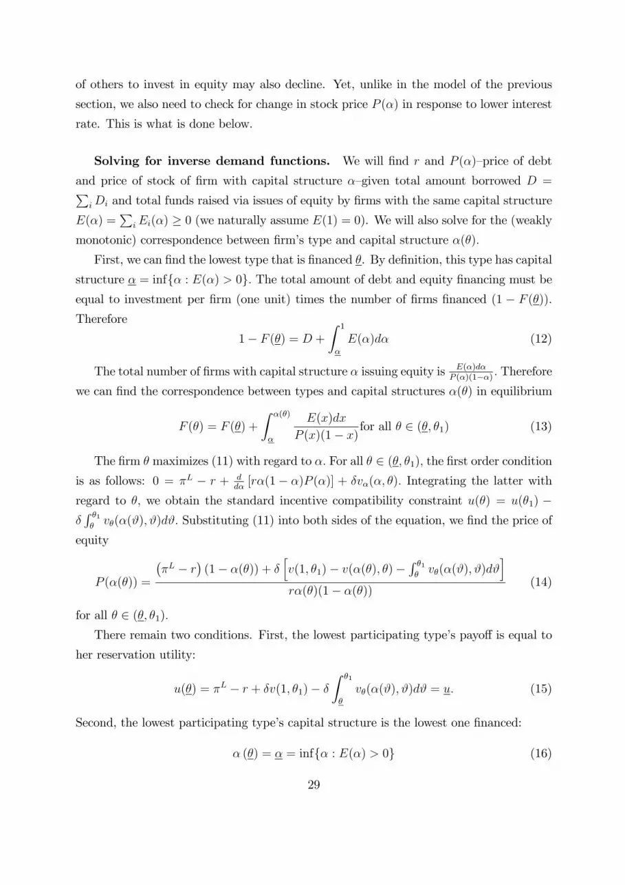
structure � = inff� : E(�) > 0g: The total amount of debt and equity �nancing must beequal to investment per �rm (one unit) times the number of �rms �nanced (1 � F (�)).Therefore

1� F (�) = D +Z 1

�

E(�)d� (12)

The total number of �rms with capital structure � issuing equity is E(�)d�P (�)(1��) : Therefore

we can �nd the correspondence between types and capital structures �(�) in equilibrium

F (�) = F (�) +

Z �(�)

�

E(x)dx

P (x)(1� x) for all � 2 (�; �1) (13)

The �rm � maximizes (11) with regard to �: For all � 2 (�; �1); the �rst order conditionis as follows: 0 = �L � r + d

d�[r�(1� �)P (�)] + �v�(�; �): Integrating the latter with

regard to �; we obtain the standard incentive compatibility constraint u(�) = u(�1) ��R �1�v�(�(#); #)d#: Substituting (11) into both sides of the equation, we �nd the price of

equity

P (�(�)) =

��L � r

�(1� �(�)) + �

hv(1; �1)� v(�(�); �)�

R �1�v�(�(#); #)d#

ir�(�)(1� �(�)) (14)

for all � 2 (�; �1):There remain two conditions. First, the lowest participating type�s payo¤ is equal to

her reservation utility:

u(�) = �L � r + �v(1; �1)� �Z �1

�

v�(�(#); #)d# = u: (15)

Second, the lowest participating type�s capital structure is the lowest one �nanced:

� (�) = � = inff� : E(�) > 0g (16)

29

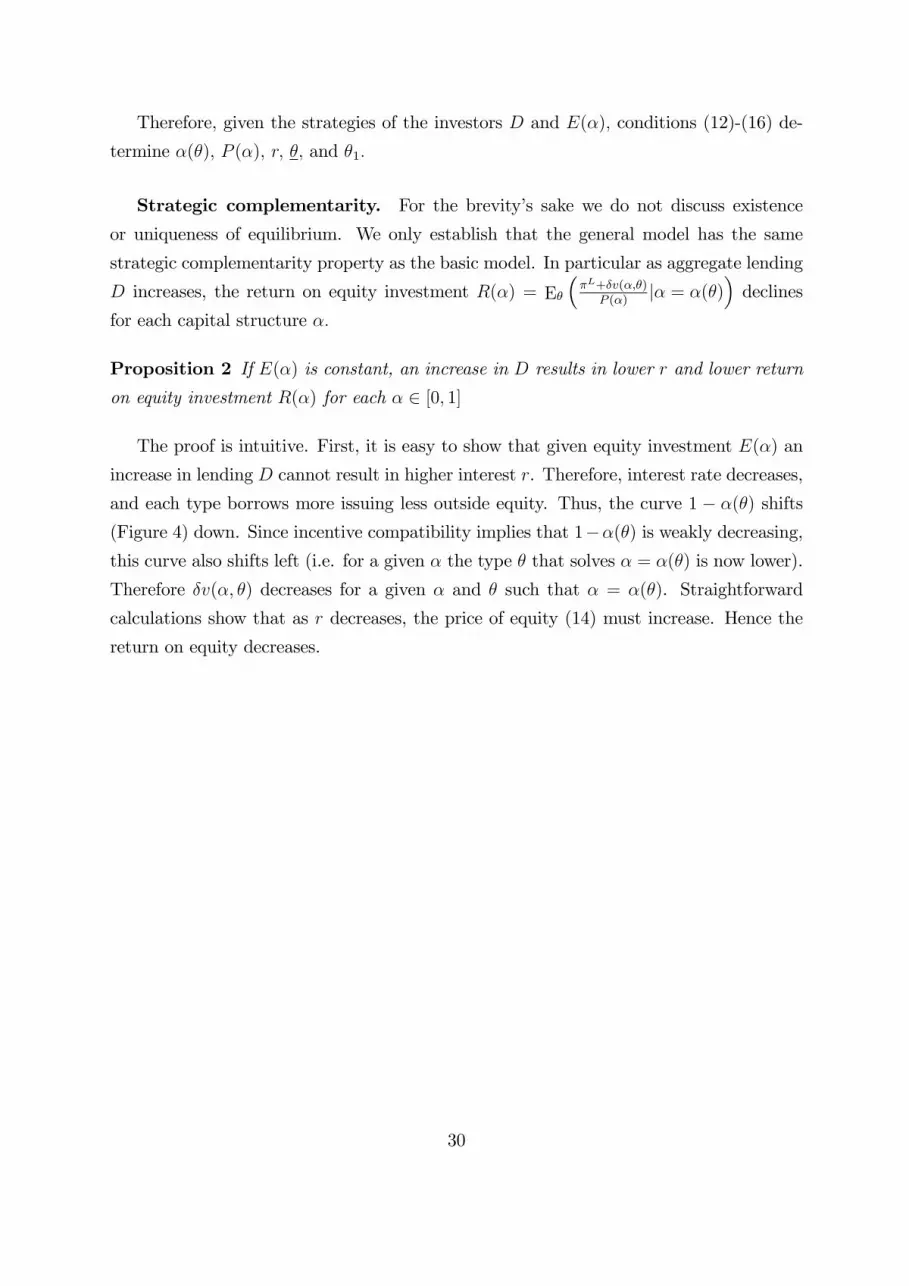
Therefore, given the strategies of the investors D and E(�); conditions (12)-(16) de-

termine �(�); P (�); r; �; and �1:

Strategic complementarity. For the brevity�s sake we do not discuss existence

or uniqueness of equilibrium. We only establish that the general model has the same

strategic complementarity property as the basic model. In particular as aggregate lending

D increases, the return on equity investment R(�) = E�

��L+�v(�;�)

P (�)j� = �(�)

�declines

for each capital structure �:

Proposition 2 If E(�) is constant, an increase in D results in lower r and lower return

on equity investment R(�) for each � 2 [0; 1]

The proof is intuitive. First, it is easy to show that given equity investment E(�) an

increase in lending D cannot result in higher interest r. Therefore, interest rate decreases,

and each type borrows more issuing less outside equity. Thus, the curve 1 � �(�) shifts(Figure 4) down. Since incentive compatibility implies that 1��(�) is weakly decreasing,this curve also shifts left (i.e. for a given � the type � that solves � = �(�) is now lower).

Therefore �v(�; �) decreases for a given � and � such that � = �(�). Straightforward

calculations show that as r decreases, the price of equity (14) must increase. Hence the

return on equity decreases.

30

References

Abreu, Dilip, and Marcus Brunnermeier (2003). �Bubbles and Crashes.�

Econometrica, 71(1), 173-204.

Allen, Franklin and Douglas Gale (2003). �Financial Fragility, Liquidity, and

Asset Prices.�Wharton Financial Institutions Center Working Paper 01-37-B.

Asparouhova, Elena (2006). �Competition in Lending: Theory and Experi-

ments,�Review of Finance, 10 (2), 189-219.

Baker, Malcolm, and Jeffrey Wurgler (2002). �Market Timing and Capital

Structure.�Journal of Finance, 57(1), 1-32.

Boot, Arnoud, and Anjan Thakor (1993). �Security design.� Journal of Fi-

nance, 48(4), 1349-1378.

Bolton, Patrick, and Xavier Freixas (2000). �Equity, Bonds, and Bank Debt:

Capital Structure and Financial Equilibrium Under Asymmetric Information.� Journal

of Political Economy, 108(2), 324-351.

Biais, Bruno, David Martimort, and Jean-Charles Rochet (2000). �Com-

peting mechanisms in a common value environment�, Econometrica, 68(4), 799�839.

Brunnermeier, Marcus (2001). Asset Pricing under Asymmetric Information �

Bubbles, Crashes, Technical Analysis, and Herding. Oxford University Press.

Bradley, Michael, Gregg Jarrell, and Han Kim (1984). �On the Existence

of Optimal Capital Structure: Theory and Evidence.� Journal of Financy, 39(3), 857-878.

Bulow, Jeremy, John Geanakoplos, and Paul Klemperer (1985). �Multi-

market Oligopoly: Strategic Substitutes and Complements.� Journal of Political Econ-

omy, 93(3), 488-511.

Calomiris, Charles W. (2002). �Banking Approaches the Modern Era.�Regula-

tion. Summer 2002, 14-20.

Chen, Hsuan-Chi, and Jay Ritter (2000). �The Seven Percent Solution.�Jour-

nal of Finance 55, 1105-1131.

Cooney, John, and Avner Kalay (1993). �Positive Information from Equity

Issue Announcements,�Journal of Financial Economics, 33(2), 149-172.

Degryse, Hans, Luc Laeven, Steven Ongena (2007). �The Impact of Organi-

zational Structure and Lending Technology on Banking Competition.�CEPR Discussion

Paper 6412.

Dell Ariccia, Giovanni, Ezra Friedman, and Robert Marquez (1999).

�Adverse selection as a barrier to entry in the banking industry.� RAND Journal of

31

Economics, 30(3), 515-534.

Dybvig, Philip, and Jaime Zender (1991). �Capital Structure and Dividend

Irrelevance with Asymmetric Information,�Review of Financial Studies, 4(1), 201-19.

Fama, Eugene, and Kenneth French (2002). �Testing Trade-O¤ and Pecking

Order Predictions about Dividends and Debt.�Review of Financial Studies, 15(1), 1-33.

Fama, Eugene, and Kenneth French (2005). �Financing Decisions: Who Issues

Stock?�Journal of Financial Economics, 76, 549-82.

Faulkender, Michael, and Mitchell A. Petersen (2006). �Does the Source

of Capital A¤ect Capital Structure?�Review of Financial Studies, 19(1), 45-79

Fulghieri, Paolo, and Dmitry Lukin (2001). �Information Production, Dilution

Costs, and Optimal Security Design.� Journal of Financial Economics, 61(1), 3-42.

Graham, John (2000). �How Big are the Tax Bene�ts of Debt?�, Journal of Finance

55, 1901-1941.

Griffith, Sean (2006). �Price Discrimination in Initial Public O¤erings.�in Helen

Perry, ed., Law and Regulation of Primary Securities Markets. Richmond Law and Tax.

Guriev, Sergei and Dmitry Kvassov (2004). �Barter for price discrimination�,

International Journal of Industrial Organization, 22(3), 329-350.

Jensen, Michael, and William Meckling (1976). �Theory of the Firm: Man-

agerial Behavior, Agency Costs and Ownership Structure.� Journal of Financial Eco-

nomics, 3(4), 305-60.

Kreps, David, and Jose Scheinkman (1983). �Quantity Precommitment and

Bertrand Competition Yield Cournot Outcomes.�The Bell Journal of Economics, 14(2),

pp. 326-337.

La Porta, Rafael, Florencio Lopez-de-Silanes, Andrei Shleifer, and

Robert W. Vishny (1998). �Law and Finance.�Journal of Political Economy, 106(6),pp.

1113-1155.

Leary, Mark, and Michael Roberts (2007). �The Pecking Order, Debt Capac-

ity, and Information Asymmetry,�Available at SSRN: http://ssrn.com/abstract=555805.

Mayer, Colin, and Oren Sussman (2004). �A New Test of Capital Structure.�

CEPR Discussion Paper 4239, London.

Modigliani, Franco, and Merton Miller (1958). �The Cost of Capital, Cor-

porate Finance, and the Theory of Investment.� American Economic Review, 48(4),

261-97.

Morrison, Alan, and William Wilhelm (2007). Investment Banking: Institu-

32

tions, Politics, and Law. Oxford University Press.

Myers, Stewart (2000). �Capital Structure.�Journal of Economic Perspectives,

15(2), 81-102.

Myers, Stewart, and Nicholas Majluf (1984). �Corporate Financing and In-

vestment Decisions When Firms Have Information That Investors Do Not Have.� Journal

of Financial Economics, 13(2), 187-221.

Oren, Shmuel, Stephen Smith and Robert Wilson (1983). �Competitive

Nonlinear Tari¤s�, Journal of Economic Theory, 29, pp.49-71.

Petersen, Mitchell, and Raghuram Rajan (1994). �The Bene�ts of Lending

Relationships: Evidence from Small Business Data.�Journal of Finance, 110(2), 407-443.

Petersen, Mitchell, and Raghuram Rajan (1995). �The E¤ect of Credit

Market Competition on Lending Relationships.�Quarterly Journal of Economics, 110(2),

407-443.

Smith, Randall (1999). �IPO Firms Face Probe of 7% Fee �US Antitrust Group

Questions a Standard,�The Wall Street Journal, May 3, C1.

Torstila, Sami (2003). �The clustering of IPO gross spreads: International evi-

dence.�Journal of Financial and Quantitative Analysis; 38 (3), 673-694.

Welch, Ivo (2004). �Capital Structure and Stock Returns.� Journal of Political

Economy, 112(1), 106-131.

33