Full Terms & Conditions of access and use can be found athttp://www.tandfonline.com/action/journalInformation?journalCode=raec20

Download by: [Oklahoma State University] Date: 23 September 2015, At: 10:15

Applied Economics

ISSN: 0003-6846 (Print) 1466-4283 (Online) Journal homepage: http://www.tandfonline.com/loi/raec20

Competition and price dispersion in the airlinemarkets

Durba Chakrabarty & Levent Kutlu

To cite this article: Durba Chakrabarty & Levent Kutlu (2014) Competition andprice dispersion in the airline markets, Applied Economics, 46:28, 3421-3436, DOI:10.1080/00036846.2014.931919

To link to this article: http://dx.doi.org/10.1080/00036846.2014.931919

Published online: 25 Jun 2014.

Submit your article to this journal

Article views: 243

View related articles

View Crossmark data

Citing articles: 1 View citing articles

Competition and price dispersion in

the airline markets

Durba Chakrabartya and Levent Kutlub,*aDepartment of Economics and Legal Studies, Oklahoma State University,Stillwater, OK 74074, USAbSchool of Economics, Georgia Institute of Technology, Atlanta, GA 30332, USA

We use two ticket-level data sets on one-way domestic flights for the US airlines toexamine the potentially nonlinear relationship between price dispersion and threeforms of competition: inter-firm, inter-flight and frequency competitions. The linearrelationship is rejected at any conventional significance levels. In particular, there isan S-shaped relationship between market concentration and price dispersion. Thiscan be a reason for the mixed results in the literature. Roughly speaking, the inter-flight and frequency competitions have opposite effects on price dispersion. Finally,in general, the size of aircraft has a positive effect on price. However, for very largeaircraft, the relationship becomes negative.

Keywords: airlines; competition; price dispersion

JEL Classification: D40; L10; L93

I. Introduction

The relationship between price dispersion and marketconcentration has been the subject of considerable numberof empirical studies. Borenstein and Rose (1994), Stavins(2001), Giaume and Guillou (2004) and Gaggero and Piga(2011) have demonstrated a negative relationship betweenprice dispersion and market concentration, while Gerardiand Shapiro (2009) have shown a positive relationship.1

However, Roos et al. (2010) found out an ambiguousrelationship between these two. So, an important questionis why we get a mixture of results involving the relationbetween price dispersion and market concentration. Onepotential answer is that all these studies in airline industrythat have been done so far concentrated only on the linearrelationship between these variables. Dai et al. (2014)have found a nonmonotonic inverse U-shaped relationshipbetween price dispersion and market power both

theoretically and empirically. Our article delves on thenonlinear relationship between other key variables thataffect price dispersion in addition to the nonlinear relation-ship of price dispersion and market concentration. Amongthese variables, we include two proxies which measureinter-flight and frequency competitions. Hence, our focusof study is also on other forms of competition besidesinter-firm competition as measured by market concentra-tion. Moreover, our data sets enable us to control manyimportant factors which could not be controlled because ofdata limitations in Dai et al. (2014).

The airlines employ different pricing strategies by offer-ing customers a range of tickets with different characteris-tics and restrictions. Hence, airlines price discriminateamong the travellers based on their individual preferences.They can offer a discount for the tickets purchased inadvance (known as advance purchase discounts), minimumstay requirements, round trip restrictions, Saturday night

*Corresponding author. E-mail: levent.kutlu@econ.gatech.edu1Kutlu andWang (2014) show a positive relationship between a conduct parameter measure of market power and price dispersion. Theyargue that the choice of market power measure may matter. However, we do not have a proper data set to estimate airline-specificconducts. For some details on conduct parameter models for market power in the airline settings, see Bresnahan (1989), Perloff et al.(2007) and Kutlu and Sickles (2012).

Applied Economics, 2014Vol. 46, No. 28, 3421–3436, http://dx.doi.org/10.1080/00036846.2014.931919

© 2014 Taylor & Francis 3421

Dow

nloa

ded

by [

Okl

ahom

a St

ate

Uni

vers

ity]

at 1

0:15

23

Sept

embe

r 20

15

stay over requirements and nonrefundable tickets as con-sidered by Gale and Holmes (1993), Dana, (1998), Stavins(2001) and Gerardi and Shapiro (2009). Thus, airlinesdesign such ticket restrictions as fencing devices to separatebusiness travellers who have low elasticity of demand andalso are time bound and less flexible as compared withleisure travellers. In this article, we consider two types ofprice dispersions. The first one is price dispersion caused byticket restrictions. We concentrate on restrictions based onnonrefundability. Once such tickets are purchased, the tra-veller cannot get his money back. Thus, the business tra-vellers who have higher valuation of time go in forrefundable options, which give them the flexibility in theirschedule of flights. Refundable tickets are unrestricted tick-ets and individuals have to pay extra money for releasingthe no-money-back restriction. The second type that weconsider is the inter-temporal price dispersion. The inter-temporal price discrimination is a major reason for this typeof price dispersion. The business travellers whose plans aregenerally at lastmoment have less elastic demand, while thetourists whose plans are flexible have relativelymore elasticdemand. Therefore, the airlines can group travellers basedon the day they want to buy a particular airline seat. Thisenables the airline to charge higher prices to high valuationtravellers based on their desired travel days, which leads toan inter-temporal dispersion in prices.

Our estimates indicate that there is no simple linearrelationship between market concentration and price dis-persion. More precisely, when the market concentration islow or high, there is a positive relationship between mar-ket concentration and price dispersion. In this range, therelationship agrees with the one suggested by Gerardi andShapiro (2009). However, for the medium values of mar-ket concentration, the relationship is negative, which is inline with the findings of Borenstein and Rose (1994) andStavins (2001). This can be a reason for the mixed resultsin the literature. The effects of inter-flight and frequencycompetitions on price dispersion are monotonic yet non-linear. The former is positively related and the latter isnegatively related to price dispersion. Hence, they haveopposite effects on price dispersion. Finally, in general,the size of aircraft has a positive effect on price. However,for very large aircraft, the relationship becomes negative.

An important feature of our article is the detailednature of our hand-collected data sets in terms of thevariables that are used. We use two data sets in ouranalysis. One of them is for price dispersion by refund-ability and the other is for inter-temporal price disper-sion. Prominent empirical studies that have been done sofar have obtained their data from the Databank of theDepartment of Transportation’s Origin and DestinationSurvey of Bureau of Transportation Statistics (BTS) as inBorenstein and Rose (1994) and Gerardi and Shapiro

(2009). Further, additional information about route char-acteristics is obtained from BTS T-100 DomesticSegment Database. These data sets do not contain infor-mation about date and time of departure, date and time ofarrival, ticket restrictions and so on. However, our handcollected data sets, like De Roos et al. (2010), have allsuch information.

As in Stavins (2001), we use data sets on individualticket prices and restrictions across US-based routes. Theadvantage of working with ticket level is providing a moreaccurate explanation for the shadow cost of airfares com-pared with earlier studies. The variation in airfares caneither be due to differences in cost (cost-based) or due toprice discrimination. So, we need to clarify between pricediscrimination and price dispersion. In this study, pricedispersion refers to the differences in prices charged to thetravellers on the same airline and route, and price discri-mination refers to such differences that are not cost-based.Therefore, when examining discriminatory practices bythe airlines in our article, those factors that affect airlineprices due to differences in costs should be controlled.

We describe our data and discuss the variables used inour estimations in Section II. Section III presents ourmodels and results and Section IV makes our conclusion.

II. Description of Data

Our study uses two hand-collected data sets of airfares toexamine price dispersion in the US domestic airline indus-try. The first data set calculates price dispersion throughticket restrictions and the second one calculates pricedispersion through inter-temporal price differences. Wecall these data sets as ‘refund’ and ‘inter-temporal’,respectively.

The refund data set includes ticket-level data on non-stop one-way first class and economy class travel forflights on 22 different directional routes operating on thesame day, Wednesday, 7 December 2011. The routes arelisted in Table 1.2 The number of observations in this dataset is 2713. The choice of city-pairs was done on the basisof nonstop flights. Many of the city-pairs are chosen sothat there is a single airport at each end. We have chosenboth first-class and economy-class travel to capture con-sumer heterogeneity since the first-class travellers areoffered a greater range and standard of service than theeconomy-class travellers and hence the first-class travel-lers are willing to pay higher costs associated with theseservices. The specific date was chosen to avoid peak holi-days as well as weekend travel. Further, we have selected asingle day to avoid price differences because of travel ondifferent days of the week. Also, the data were collectedon the thirty-fifth, twenty-first, fourteenth and second day

2To save space, we provide only the city-pair names that constitute the directional routes.

3422 D. Chakrabarty and L. Kutlu

Dow

nloa

ded

by [

Okl

ahom

a St

ate

Uni

vers

ity]

at 1

0:15

23

Sept

embe

r 20

15

before the scheduled travel date to get an idea about theprices offered prior to the departure date. This data set usesdata collected from an online site (Expedia), which com-prises domestic airfares of major US airlines. With variousonline travel agencies, the consumers have the ease ofsearching and comparing prices. The preliminary data con-tain airline information like origin airport, destination air-port, origin city, destination city, flight number, price, tax,total price (inclusive of all taxes and surcharges), departuretime, distance, duration and aircraft size (flight-specificnumber of seats).3 Based on the above information, wehave constructed a variety of dummy variables such asAMPEAK, PMPEAK, FIRST, REFUND, FIRMDUMMIES, SOLD, HUB, OD, BIGCITY and LCC. Thevariables DIST and DISTSQ represent minimum flightdistance between two endpoint airports (in miles) and itssquare, respectively. For visual purposes, in our regressionoutputs, DIST is divided by 1000. Hence, the unit of DISTvariable is 1000 miles. DUR and DURSQ represent theflight duration in number of hours. AMPEAK stands fordummy variable, which is equal to one for the morning timeperiod (6:30 am–8:30 am), and similarly PMPEAK is adummy variable for the evening peak time (4:30 pm–6:30pm). We have another dummy variable OD (operatingdummy), which equals to one when the marketing and theoperating firm are different. FIRST and REFUND aredummy variables equal to one for first-class tickets andrefundable tickets, respectively. SOLD stands for adummy variable which is equal to one only for the observa-tion just before the ticket disappears. For example, if the

ticket is sold out on the second day before the flight, thenthe sold dummy on fourteenth day will be equal to one andthe rest of them, that is, on thirty-fifth day and twenty-firstday are equal to zero. Of course, in this case, we do not havean observation for the second day. HUB is a dummy vari-able equal to one if either the origin or the destinationairport is a hub for the airline. LCC is a dummy variablewhich is equal to one for a route having at least one low costcarrier serving a nonstop flight on that route. The low costcarriers that determine the LCC variable are AirTranAirways, Frontier Airlines, JetBlue Airways andSouthwest Airlines. AP, APSQ and APCU stand for thenumber of days in advance the tickets are purchased beforethe actual flight date, its square and its cube, respectively.TNF, TNFSQ and TNFCU correspond to the total numberof flights, its square and its cube, respectively. Also, ASNF,ASNFSQ and ASNFCU are the firm-specific number offlights, its square and its cube, respectively. In our regres-sion outputs, TNF and ASNF are divided by 100. Whenmore than one airline shares the same flight, ASNF for theseairlines are increased by reciprocal of the number of airlinessharing the flight. For example, if two airlines share a flight,then this flight would increase ASNF of each airline by half.Another important variable is the SIZE, which stands forthe aircraft size. SIZESQ and SIZECU represent the squareand cube of SIZE, respectively. In our regression outputs,SIZE is divided by 100. Hence, the unit of SIZE variable is100 seats. The variable SHARE represents the market shareof each of the firms on a given route and is based on theavailable number of seats of each airline on a given route.The formula is:

SHARE ¼ number of seats of each airline=

total number of seats of all the airlines

Hirschman Herfindahl Index (HHI) has been con-structed to measure market concentration. It is the sumof squares of market shares and ranges from 0 to 1. We usethe available number of seats on a route to calculate air-lines’ market shares and market structure (as measured byHHI) instead of using the number of flights or the numberof carriers on a route as a basis for market concentrationcalculations. HHISQ and HHICU denote the square andcube of HHI, respectively. TEMPO and TEMPD corre-spond to the mean temperature (in Fahrenheit) in originand destination for December. At first, we considered theTEMP = TEMPD − TEMPO variable similar to Stavins(2001), where she has considered the absolute differencein mean January temperatures as a proxy for tourismbetween origin and destination. However, the TEMP vari-able captures only the size of tourist people but does not

Table 1. Routes and airlines for refund data set

City-pair Distance Airlines

Atlanta Baltimore* 578 FL, DLAtlanta Memphis 332 FL, DLBoston Cleveland 562 CO, UABoston Tampa 1185 B6Baltimore Philadelphia 90 USCleveland Charlotte 430 US, UA, COCharlotte Memphis 512 DL, USCincinnati Newark 580 UA, CO, DLDenver Las Vegas* 609 F9, UA, CODenver Phoenix* 590 US, UA, COPhiladelphia Tampa* 920 US, UA

Notes: A route is defined as a flight conducted between origincity and destination city. We list 11 city-pairs each with bothdirections making up 22 directional routes. The airlines havebeen named according to BTS airline code where CO:Continental, UA: United, DL: Delta, B6: Jet Blue, FL: AirTran,F9: Frontier, and US: US Airways. Bolded routes are consideredto be LCC routes. Routes in which Southwest provides nonstopservice are denoted by *.

3 For each ticket, the model of the aircraft is known. However, because of potential modifications, the actual numbers can differ. Becauseof difficulties in data collection procedure, we used the number of seats for unmodified aircraft.

Competition and price dispersion in the airline markets 3423

Dow

nloa

ded

by [

Okl

ahom

a St

ate

Uni

vers

ity]

at 1

0:15

23

Sept

embe

r 20

15

capture the relative sizes of tourist and the business peo-ple. Hence, we generated a new variable RFIRSTSHARE,which aims to overcome this issue. It stands for route first-class share variable and gives us the share of available firstclass seats on a route. It is calculated by dividing thenumber of available first class seats on a route by thenumber of available seats. The purpose of this variable iscapturing the heterogeneity of the routes. Although we donot know the real tourist/business people ratio, we can usethis variable as a proxy. The variable DIFFGAMBLErepresents the difference in the number of gambling insti-tutions between destination and origin. The state ofNevada has the largest number of gambling propertiesand the city of Las Vegas has the major share. BIGCITYis a dummy variable equal to one if the destination is a bigcity and not the origin. The variables POPO and POPDrepresent the population in 2010 in origin and destination,respectively. Similarly, PCIO and PCID stand for per-capita money income in origin and destination, respec-tively. POPO, POPD, PCIO and PCID have been collectedfrom US Census Bureau. Based on the above information,we constructed a set of other variables. The variable POP isthe average population for the city-pair in 1 000 000 s (ofpeople). That is, POP = (POPO + POPD)/2. The variablePCI stands for population weighted per capita income in$1000s. That is, PCI = (POPO × PCIO + POPD × PCID)/(POPO + POPD). POPPCI is the cross product of POP andPCI. The variables REFHHI, REFHHISQ, REFHHICU,REFTNF, REFTNFSQ, REFTNFCU, REFASNF,REASNFSQ, REFASNFCU, REFSIZE, REFSIZESQ,REFSIZECU, REFAP, REFAPSQ and REFAPCU repre-sent the cross products of REFUND and the relevant vari-ables. DISTSOLD stands for the cross product of DISTandSOLD. Finally, lnP stands for the logarithm of ticket price.

The inter-temporal data set includes the ‘minimum ticketprice’ data in a given day on one-way economy class travelfor flights on 417 different directional routes operating onthe same day, Tuesday, 20 November 2012. Unlike therefund data set, this data set includes tickets with up tothree stops. The number of observations in the final dataset is 86 142. This data set contains ticket information for alarger number of airlines. In particular, the airlines includedin this data set are American Airlines (AA), Alaska Airlines(AS), JetBlue Airways (B6), Delta Airlines (DL), FrontierAirlines (F9), AirTran Airways (FL), Spirit Airlines (NK),Sun Country Airlines (SY), United Airlines (UA), USAirways (US) and Virgin America (VX). Among theseairlines, the low cost carriers are JetBlue Airways (B6),Frontier Airlines (F9), AirTran Airways (FL), SpiritAirlines (NK), Sun Country airlines (SY) and Virgin

America (VX). As earlier, the LCC dummy includes allthese airlines as well as Southwest Airlines. The initial datawere collected on the twenty-ninth, twenty-second, fif-teenth, eighth and first day before the scheduled traveldate to get an idea about the prices offered prior to thedeparture date. Then, for any given number of stops andfor each flight, the minimum, PMIN, and maximum,PMAX, of the prices are calculated.4 Hence, two ticketsbetween the same city-pair with different number of stopsare treated separately when finding the minimum and max-imum prices. The ticket prices are obtained from the meta-search engine of Kayak web site, which searches the onlinesites: Priceline, Travelocity, Expedia, CheapOair,OneTravel and airline specific websites. The relevant vari-ables in this data set are generated similar to their refunddata set counterparts. The additional variables in this dataset are STOP, PDI, SOLDALL and DISTSOLDALL.STOP variable is the number of stops for an itinerary andPDI = PMAX/PMIN stands for inter-temporal price disper-sion. We call this inter-temporal price dispersion as it mea-sures the price variation over time. Since the inter-temporaldata set does not have time-dependent observations, theSOLD variable cannot be defined.5 Hence, we define asimilar variable, which we call SOLDALL. This variableis equal to one if the tickets for a flight are sold out the daybefore (or earlier) the flight. DISTSOLDALL variable is theproduct of DIST and SOLDALL variables. The descriptivestatistics for our data sets are given in Table 2.

III. Models and Results

In this section, we present our models and results. Weconsider two sets of estimates. The first set of estimatesis based on the refund data set and the second one is basedon the inter-temporal data set. These data sets enable us toexamine the price dispersion from different perspectives.We present the models and estimation results in the fol-lowing subsections.

Price dispersion by refundabilty model

There are at least two ways to price discriminate: setting theticket prices as a function of refundability and/or the time ofpurchase. The resulting price dispersion types are pricedispersion by refundability and inter-temporal price disper-sion, respectively. This section concentrates on price dis-persion by refundability. The models for the refund data setand estimates are presented in Tables 3 and 4.

4Note that, for the inter-temporal data set, the prices are already minimum prices for a given day. Hence, PMIN and PMAX are theminimum and maximum of these minimum prices over time, respectively. This is in line with the approach used by Gillen and Hazledine(2012) who examine price discrimination. See also Hazledine (2011) for a similar setup using inter-temporal minimal prices for airlines.5Remember that the prices for the inter-temporal data set are the minimum and maximum prices over time.

3424 D. Chakrabarty and L. Kutlu

Dow

nloa

ded

by [

Okl

ahom

a St

ate

Uni

vers

ity]

at 1

0:15

23

Sept

embe

r 20

15

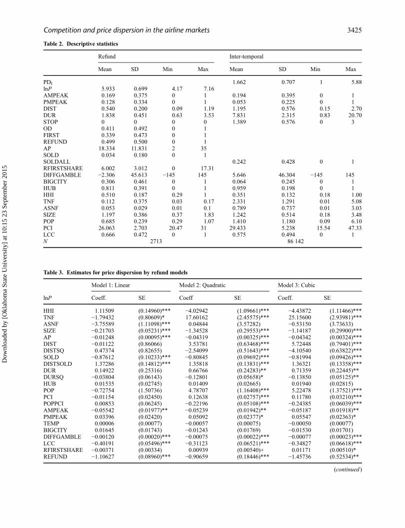
Table 3. Estimates for price dispersion by refund models

Model 1: Linear Model 2: Quadratic Model 3: Cubic

lnP Coeff. SE Coeff SE Coeff. SE

HHI 1.11509 (0.14960)*** −4.02942 (1.09661)*** −4.43872 (1.11466)***TNF −1.79432 (0.80609)* 17.60162 (2.45575)*** 25.15600 (2.93981)***ASNF −3.75589 (1.11098)*** 0.04844 (3.57282) −0.53150 (3.73633)SIZE −0.21703 (0.05231)*** −1.34528 (0.29553)*** −1.14187 (0.29900)***AP −0.01248 (0.00095)*** −0.04319 (0.00325)*** −0.04342 (0.00324)***DIST −0.01122 (0.86066) 3.53781 (0.63468)*** 5.72448 (0.79401)***DISTSQ 0.47374 (0.82655) −2.54099 (0.51643)*** −4.10540 (0.63822)***SOLD −0.87612 (0.10233)*** −0.80845 (0.09692)*** −0.81994 (0.09426)***DISTSOLD 1.37286 (0.14812)*** 1.35818 (0.13831)*** 1.36321 (0.13358)***DUR 0.14922 (0.25316) 0.66766 (0.24283)** 0.71359 (0.22445)**DURSQ −0.03804 (0.06143) −0.12801 (0.05658)* −0.13850 (0.05125)**HUB 0.01535 (0.02745) 0.01409 (0.02665) 0.01940 (0.02815)POP −0.72754 (1.50736) 4.78707 (1.16408)*** 5.22478 (1.37521)***PCI −0.01154 (0.02450) 0.12638 (0.02757)*** 0.11780 (0.03210)***POPPCI 0.00853 (0.06245) −0.22196 (0.05108)*** −0.24385 (0.06039)***AMPEAK −0.05542 (0.01977)** −0.05239 (0.01942)** −0.05187 (0.01918)**PMPEAK 0.03396 (0.02420) 0.05092 (0.02377)* 0.05547 (0.02363)*TEMP 0.00006 (0.00077) −0.00057 (0.00075) −0.00050 (0.00077)BIGCITY 0.01645 (0.01743) −0.01243 (0.01769) −0.01530 (0.01701)DIFFGAMBLE −0.00120 (0.00020)*** −0.00075 (0.00022)*** −0.00077 (0.00023)***LCC −0.40191 (0.05496)*** −0.31123 (0.06521)*** −0.34827 (0.06618)***RFIRSTSHARE −0.00371 (0.00334) 0.00939 (0.00540)+ 0.01171 (0.00510)*REFUND −1.10627 (0.08960)*** −0.90659 (0.18446)*** −1.45736 (0.52534)**

(continued )

Table 2. Descriptive statistics

Refund Inter-temporal

Mean SD Min Max Mean SD Min Max

PDI 1.662 0.707 1 5.88lnP 5.933 0.699 4.17 7.16AMPEAK 0.169 0.375 0 1 0.194 0.395 0 1PMPEAK 0.128 0.334 0 1 0.053 0.225 0 1DIST 0.540 0.200 0.09 1.19 1.195 0.576 0.15 2.70DUR 1.838 0.451 0.63 3.53 7.831 2.315 0.83 20.70STOP 0 0 0 0 1.389 0.576 0 3OD 0.411 0.492 0 1FIRST 0.339 0.473 0 1REFUND 0.499 0.500 0 1AP 18.334 11.831 2 35SOLD 0.034 0.180 0 1SOLDALL 0.242 0.428 0 1RFIRSTSHARE 6.002 3.012 0 17.31DIFFGAMBLE −2.306 45.613 −145 145 5.646 46.304 −145 145BIGCITY 0.306 0.461 0 1 0.064 0.245 0 1HUB 0.811 0.391 0 1 0.959 0.198 0 1HHI 0.510 0.187 0.29 1 0.351 0.132 0.18 1.00TNF 0.112 0.375 0.03 0.17 2.331 1.291 0.01 5.08ASNF 0.053 0.029 0.01 0.1 0.789 0.737 0.01 3.03SIZE 1.197 0.386 0.37 1.83 1.242 0.514 0.18 3.48POP 0.685 0.239 0.29 1.07 1.410 1.180 0.09 6.10PCI 26.063 2.703 20.47 31 29.433 5.238 15.54 47.33LCC 0.666 0.472 0 1 0.575 0.494 0 1N 2713 86 142

Competition and price dispersion in the airline markets 3425

Dow

nloa

ded

by [

Okl

ahom

a St

ate

Uni

vers

ity]

at 1

0:15

23

Sept

embe

r 20

15

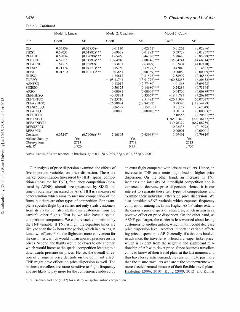
Our analysis of price dispersion examines the effects offive important variables on price dispersion. These aremarket concentration (measured by HHI), spatial compe-tition (measured by TNF), frequency competition (mea-sured by ASNF), aircraft size (measured by SIZE) andtime of purchase (measured by AP).6 HHI is a measure ofconcentration which aims to measure competition of thefirms, but there are other types of competition. For exam-ple, a specific flight by a carrier not only steals customersfrom its rivals but also steals own customers from thecarrier’s other flights. That is, we also have a spatialcompetition component. We capture such competition bythe TNF variable. If TNF is high, the departure times arelikely to span the 24 hour time period, which in turn has, atleast, two effects. First, the flights are more convenient forthe customers, which would put an upward pressure on theprices. Second, the flights would be closer to one another,which would increase the spatial competition leading to adownwards pressure on prices. Hence, the overall direc-tion of change in price depends on the dominant effect.TNF might have effects on price dispersion as well. Thebusiness travellers are more sensitive to flight frequencyand are likely to pay more for the convenience induced by

an extra flight compared with leisure travellers. Hence, anincrease in TNF on a route might lead to higher pricedispersion. On the other hand, an increase in TNFincreases the intensity of inter-flight competition and isexpected to decrease price dispersion. Hence, it is ourinterest to separate these two types of competitions andexamine their individual effects on price dispersion. Wealso consider ASNF variable which captures frequencycompetition among the firms. Higher ASNF values extendthe carrier’s price dispersion strategies, which in turn has apositive effect on price dispersion. On the other hand, asASNF gets larger, the carrier is less worried about losingcustomers to another airline, which in turn could decreaseprice dispersion level. Another important variable affect-ing price dispersion is AP. Generally, if a ticket is bookedin advance, the traveller is offered a cheaper ticket price,which is evident from the negative and significant rela-tionship of AP with ticket price. Since business travellerscome to know of their travel plans at the last moment andthus have less elastic demand, they are willing to pay morethan the leisure travellers who are at the other extremewithmore elastic demand because of their flexible travel plans.Hazledine (2006, 2010), Kutlu (2009, 2012) and Kumar

Table 3. Continued

Model 1: Linear Model 2: Quadratic Model 3: Cubic

lnP Coeff. SE Coeff SE Coeff. SE

OD 0.05539 (0.02855)+ 0.01130 (0.02851) 0.01262 (0.02996)FIRST 0.69031 (0.01882)*** 0.69658 (0.01893)*** 0.69729 (0.01857)***REFHHI 0.63034 (0.12090)*** 1.65460 (0.46730)*** 5.28610 (0.85729)***REFTNF 6.67115 (0.74793)*** −10.64940 (2.08246)*** −135.64741 (14.66314)***REFASNF 1.64515 (0.96899)+ 3.73881 (2.63099) 11.02404 (44.02110)REFSIZE 0.21374 (0.04171)*** 0.75250 (0.32127)* 0.42040 (0.14807)**REFAP 0.01210 (0.00111)*** 0.03851 (0.00389)*** 0.00082 (0.00009)***HHISQ 4.35617 (0.81593)*** 12.58997 (2.46862)***TNFSQ −108.13761 (13.91776)*** −60.58258 (6.20452)***ASNFSQ 9.13012 (42.77480) 4.01568 (5.69128)SIZESQ 0.50125 (0.14680)*** 0.24286 (0.73144)APSQ 0.00081 (0.00009)*** 0.04760 (0.00889)***REFHHISQ −0.93893 (0.33667)** −18.91787 (4.20830)***REFTNFSQ 79.23710 (8.51493)*** 626.71009 (65.07037)***REFASNFSQ −26.90084 (22.94592) 0.78396 (112.54489)REFSIZESQ −0.26597 (0.15905)+ −0.01157 (0.67049)REFAPSQ −0.00070 (0.00010)*** −0.00134 (0.00063)*REFHHICU 9.10555 (2.20661)***REFTNFCU −1,765.21822 (208.36137)***REFASNFCU −339.76329 (667.08259)REFSIZECU −0.02438 (0.19792)REFAPCU 0.00001 (0.00001)Constant 6.05247 (0.79006)*** 2.10503 (0.63968)** 1.09491 (0.79819)Airline Dummy Yes Yes YesObservations 2713 2713 2713Adj. R2 0.726 0.751 0.757

Notes: Robust SEs are reported in brackets. +p < 0.1, *p < 0.05, **p < 0.01, ***p < 0.001.

6 See Escobari and Lee (2012) for a study on spatial airline competition.

3426 D. Chakrabarty and L. Kutlu

Dow

nloa

ded

by [

Okl

ahom

a St

ate

Uni

vers

ity]

at 1

0:15

23

Sept

embe

r 20

15

and Kutlu (2014) exemplify some papers that model theairline demand under this assumption. Thus, according tothese papers, the consumers’ valuations of airline seats arenegatively related with the length of time between pur-chase and flight time, such that the keenest potentialcustomers are the last minute travellers. Hence, this vari-able captures inter-temporal price dispersion. Inclusion ofthe AP variable in our model enables us to examine thelinks of price dispersion by refundability and inter-tem-poral price dispersion. A particular question we seek to

answer is whether the price of refundability falls as theflight date approaches.

In the long run, where the capacities can easily beswitched, the equilibrium prices and capacity choices aremade either jointly by the interaction of multiple sellers andbuyers or by forward looking sellers who anticipate inter-action and pricing strategies. Hence, the capacity choicesand market structure may be endogenous if the airlines areflexible in changing their capacities. Similarly, it can beargued that TNF, ASNF, SIZE and functions of these

Table 4. Estimates for price dispersion by refund models: restricted quadratic

Model 4 Model 5 Model 6 Model 7 Model 8

lnP Coeff. SE. Coeff. SE Coeff. SE Coeff. SE Coeff. SE

HHI −2.3444 (0.9655)*HHISQ 2.8788 (0.7839)***REFHHI 3.1060 (0.4390)***REFHHISQ −2.3727 (0.3279)***TNF −1.0923 (1.9348)TNFSQ −21.0897 (10.1240)*REFTNF −13.9223 (2.1028)***REFTNFSQ 95.9034 (9.1104)***ASNF −9.9840 (3.1663)**ASNFSQ 57.0578 (30.6997)+REFASNF −0.4633 (2.5220)REFASNFSQ 75.8019 (21.3062)***SIZE −1.4619 (0.2877)***SIZESQ 0.4834 (0.1433)***REFSIZE 1.2198 (0.2801)***REFSIZESQ −0.3418 (0.1418)*AP −0.0418 (0.0035)***APSQ 0.0008 (0.0001)***REFAP 0.0365 (0.0043)***REFAPSQ −0.0007 (0.0001)***DIST −0.5439 (1.5493) −2.6650 (1.8122) −4.3440 (2.6068)+ −4.4192 (1.9918)* −3.8067 (1.8601)*DISTSQ 1.1308 (1.5125) 2.8533 (1.7434) 4.5867 (2.6212)+ 4.5901 (1.9458)* 4.1591 (1.8425)*SOLD −0.8739 (0.1019)*** −0.8408 (0.0964)*** −0.8347 (0.1161)*** −0.7777 (0.1205)*** −0.7896 (0.1153)***DISTSOLD 1.4439 (0.1474)*** 1.3718 (0.1381)*** 1.4000 (0.1676)*** 1.3024 (0.1769)*** 1.3469 (0.1622)***DUR 0.1520 (0.2628) −0.2214 (0.2409) −0.0870 (0.2806) 0.0581 (0.2512) −0.2913 (0.2397)DURSQ −0.0373 (0.0624) 0.0388 (0.0589) 0.0185 (0.0665) −0.0154 (0.0581) 0.0629 (0.0559)HUB 0.0612 (0.0295)* 0.0559 (0.0275)* 0.0403 (0.0275) 0.0146 (0.0276) 0.0678 (0.0293)*POP −1.9413 (2.4014) −1.1719 (3.0861) −3.9355 (5.2039) −2.9879 (3.4883) −2.8105 (3.3674)PCI −0.0175 (0.0339) 0.0190 (0.0495) −0.0304 (0.0837) 0.0029 (0.0528) −0.0010 (0.0510)POPPCI 0.0520 (0.0979) 0.0359 (0.1257) 0.1492 (0.2151) 0.1098 (0.1439) 0.1026 (0.1392)AMPEAK −0.0504 (0.0219)* −0.0556 (0.0207)** −0.0653 (0.0216)** −0.0634 (0.0220)** −0.0652 (0.0211)**PMPEAK 0.0427 (0.0270) 0.0220 (0.0254) 0.0257 (0.0259) 0.0297 (0.0262) 0.0320 (0.0261)TEMP −0.0002 (0.0009) −0.0003 (0.0008) −0.0004 (0.0008) −0.0005 (0.0008) −0.0005 (0.0008)BIGCITY 0.0064 (0.0208) 0.0816 (0.0181)*** 0.0678 (0.0221)** 0.0917 (0.0195)*** 0.0939 (0.0193)***DIFFGAMBLE −0.0009 (0.0003)*** −0.0005 (0.0002)* −0.0004 (0.0002)* −0.0003 (0.0002) −0.0002 (0.0002)LCC −0.4462 (0.0764)*** −0.6040 (0.0757)*** −0.7980 (0.1261)*** −0.6892 (0.0926)*** −0.7919 (0.0902)***RFIRSTSHARE 0.0032 (0.0051) −0.0068 (0.0040)+ −0.0064 (0.0065) −0.0086 (0.0057) −0.0126 (0.0060)*REFUND −0.3509 (0.1314)** 0.7498 (0.1109)*** 0.2825 (0.0600)*** −0.3874 (0.1116)*** 0.1767 (0.0295)***OD 0.1022 (0.0255)*** 0.0847 (0.0245)*** 0.0939 (0.0257)*** 0.0263 (0.0308) 0.0866 (0.0262)***FIRST 0.6742 (0.0204)*** 0.6732 (0.0195)*** 0.6709 (0.0196)*** 0.6869 (0.0211)*** 0.6787 (0.0207)***Constant 6.2382 (1.2624)*** 6.2256 (1.6962)*** 7.7025 (2.6751)** 7.3393 (1.8003)*** 7.0457 (1.7167)***Airline Dummy Yes Yes Yes Yes YesObservations 2713 2713 2713 2713 2713Adj. R2 0.660 0.694 0.673 0.664 0.671

Notes: Robust SEs are reported in brackets. +p < 0.1, *p < 0.05, **p < 0.01, ***p < 0.001.

Competition and price dispersion in the airline markets 3427

Dow

nloa

ded

by [

Okl

ahom

a St

ate

Uni

vers

ity]

at 1

0:15

23

Sept

embe

r 20

15

variables may also be endogenous. In line with Stavins(2001), we assume that HHI is exogenous since we areconsidering cross section data where we encounter shortrun HHI, which is less likely to change. HHI is not affectedin the very short run by prices. It would rather be affected byprices if we consider longer time periods. Thus, there is apossibility of changing HHI in panel data where we havelong run HHI. Another explanation can be that of Grahamet al. (1983) and Stavins (2001), where different entrybarriers such as limited gate access, hub spoke systemsand scale economies create high costs of entry for the newairlines and thus prevent them from entering the airlinemarket. By similar arguments, we argue that TNF, ASNFand SIZE may be treated as exogenous variables. A poten-tial issue which could bias the results is that the size ofaircraft is correlated with the DIST variable, implying thatomitting the SIZE variable would lead to omitted variablebias as pointed out by Gerardi and Shapiro (2009).However, Borenstein and Rose (1994) and Stavins (2001)either ignored this point or did not fully capture it. In otherwords, they did not use the SIZE variable in their estima-tions but only used the DIST variable. We include the SIZEvariable to avoid this problem. Another potential issue thatcan bias the results is the lack of inventory level data in ourestimations. That is, we do not have a data on sold inventorylevels. However, the inclusion of SOLD variable would atleast partially address this potential issue. In effect, theSOLD variable is equal to one when the sold inventorylevel is very high and it is equal to zero otherwise. Finally,the airline pricing is intrinsically a dynamic problem. Ifbuyers and sellers behave dynamically during advancesales, there would be a potential danger that simple OLSmay rule out these dynamics.7 Hence, a dynamic modelmay reveal more precise information about the relationshipbetween market power and price dispersion. However, thisis beyond the scope of this study.

We measure price dispersion in terms of unrestrictedtickets and capture it by the REFUND dummy and itscross products with HHI, TNF, ASNF, SIZE, AP and thesquares and cubes of these variables. Our measure of pricedispersion is the partial derivative of (100 times) logarithmof price with respect to REFUND variable, which givesthe approximate percentage change in price due to refund.The formula for price dispersion by refund (PDR) isgiven by

PDR ¼ 100@ lnP

@REFUND

The F-test rejects the linear (Model 1) and quadratic(Model 2) models against the cubic model (Model 3) at0.001 significance level.8 Based on both quadratic andcubic models, the effect of ASNF on price dispersion isnot significant.9 Hence, in this section, we concentrateonly on HHI, TNF, SIZE and AP. The linear model pre-dicts that all HHI, TNF, SIZE and AP have positive effecton price dispersion by refundability. The estimated direc-tion of inter-firm competition (HHI) effect on price dis-persion contrasts with the estimates of Stavins (2001).This result is robust to omitting SIZE variable and itscross products with other variables from the models.Hence, although our methodology is similar to the oneused by Stavins (2001), our results disagree with herfindings. Roughly speaking, based on the refund data setestimates, with some exceptions, it seems that TNF, SIZEand AP have a positive relationship with price dispersion.However, the linear model is not capable of capturing thedirection and magnitude of price dispersion for theextreme ends of competition. In particular, the directionof the relationship between HHI and price dispersiondepends on the value of HHI. In Model 4–8, we presentthe ‘restricted quadratic’ form estimation results whereonly one factor affects price dispersion at a time. Thesemodels suggest that price dispersion is nonlinearly relatedwith HHI, TNF, SIZE and AP. In what follows, we con-centrate on the estimates from Model 3, which allowsrelatively flexible nonlinear relationships.

As expected, the ticket prices are sensitive to traveltimes, and we find that AMPEAK tends to decrease theticket prices as compared with PMPEAK, which raises theticket prices significantly. So, if a traveller picks up morn-ing flights, he would be paying less than the evening peaktraveller. The other variables explaining the cost-relatedvariation in prices are the distance (DIST) and duration(DUR) variables and their squares DISTSQ and DURSQ.DISTSQ and DURSQ are included in the model so that wecan capture the nonlinear cost structure of flights becauseof huge take off cost and other distance-related factors.Another variable that might capture the cost-related varia-tion in prices is OD. As already mentioned, OD refers to thefact that the marketing and the operating firm can be differ-ent, and this can potentially lead to a rise in costs. Thecoefficient for OD variable is positive, but it is insignificantat any conventional significance levels. In addition to thesevariables, The FIRST variable also has effect on cost-related variation in price. The coefficient of FIRST variableis significant and positive. Usually, the first-class offers agreater range and standard of service than the economy-

7 See, for example, Deneckere and Peck (2012) and Escobari (2012) for such studies.8Adjusted R2 agrees with this conclusion.9 For the quadratic model, the p-value for the joint significance of REFASNF and REFASNFSQ is 0.3260. For the cubic model, thep-value for the joint significance of REFASNF, REFASNFSQ and REFASNFCU is 0.0941.

3428 D. Chakrabarty and L. Kutlu

Dow

nloa

ded

by [

Okl

ahom

a St

ate

Uni

vers

ity]

at 1

0:15

23

Sept

embe

r 20

15

class and which in turn has higher costs. Moreover, thesetickets target business travellers who have inelasticdemand. Hence, the first-class tickets are expected to bemore expensive than the economy-class tickets.

Following Borenstein and Rose (1994), we consider twotypes of peak-load pricing: (1) systematic and (2) stochas-tic.10 Peak load pricing is affected by the shadow cost ofcapacity. The shadow cost of additional seat is higherrelative to nonpeak times, since in peak time period be itdaily or weekly, almost all of the airline aircraft are flying.The airlines know their expected utilization rates andexpected airport congestion level for the peak time periods,and this is related to the systematic-type peak load pricing.Peak hour dummies are good candidates for explaining thesystematic peak load pricing, which we have already con-sidered. Borenstein and Rose (1994) did not have data onthe flight times. Instead, they use SD of cubed airline fleetutilization rate (SDCAPFLT) and cubed SD of airportoperations rate (SDCAPAPT) to reflect the variation inshadow cost. These variables are calculated for designatedmarkets as for some of the airports, and the full capacity isnot utilized even in the peak time periods. On the otherhand, stochastic peak load pricing is related to the demanduncertainty that cannot be estimated by historical data (suchas average price, average demand, and load factor) and getsresolved only after the equipment scheduling is made. Apotential variable that may be capturing stochastic peakload pricing would be the SOLD dummy. Note that thisdummy is flight-specific and is not systematic. When thisvariable is equal to one, it is understood that the tickets areabout to sell out. This variable captures the shadow costafter the capacity choice of the airline is made. Therefore, itappears to be a fairly good variable for capturing the sto-chastic peak load pricing. However, Borenstein and Rose(1994) did not have access to such kind of data.

We consider the impact of the DISTSOLD variablealong with the SOLD variable on ticket prices. TheSOLD variable not only captures the shadow cost relatedto the stochastic peak load but also the cost due to a heavierflight load as it indicates that the flight will be full. Ourestimates show that whenever the distance is high, the ticketprices are more expensive for those flights that are close tobe sold out. Usually, for long distances when the seatsbecome scarce, the travellers have no other choices but tobuy the ticket or do not travel. So, the airlines utilize the factthat air travellers for long distance have less elastic demandcompared with short distance travellers. On the other hand,our estimates show that for the short distance flights, theticket prices are less expensive for those flights that are

close to sold out. For flights of shorter distance, the travellercan go for other options such as car, train, bus and so on,and thus the competition with other travel options forces theairlines to drop prices so as to fill otherwise empty seats.But, for long distance flights, air travel is the only optionand thus the airlines tend to raise ticket prices. So, when thedistance is high, airlines enjoy higher market power (due toreduced competition with substitutes) and hence canincrease their prices.

The RFIRSTSHARE variable is significant. The TEMPvariable is insignificant at any conventional significancelevel. TEMP variable is not significant in Stavins (2001)as well. To consider the effect of leisure travellers on ticketprices, we have constructed the gamble difference variableDIFFGAMBLE, which has a negative and significantcoefficient. Mostly, the cities which have a greater numberof gambling institutions are visited by people on leisure orentertainment trips. It is an established result that thoseroutes having low cost carriers have lower prices in gen-eral. The LCC dummy variable is used to capture the effectof presence of low cost carriers on the prices. As expected,the prices are lower when low cost carriers serve in a route.Finally, we have included POP, PCI and their cross pro-ducts POPPCI to capture city-pair-specific heterogene-ities, BIGCITY and HUB to capture big city and hubeffects, and firm dummies to capture firm-specific hetero-geneities. The coefficients of both BIGCITY and HUBdummies are insignificant. The coefficient of HUB isinsignificant in the estimates of Stavins (2001) as well.

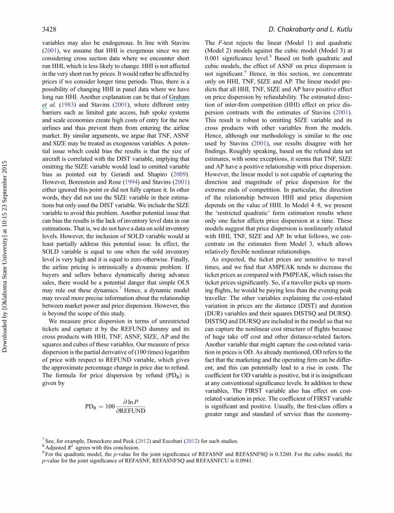
We summarize our estimates for price dispersion withthe help of four figures: (1) Price dispersion due to con-centration (HHI); (2) Price dispersion due to inter-flightcompetition (TNF); (3) Price dispersion due to aircraft size(SIZE); (4) Price dispersion due to advance purchase(AP).11 Each figure is calculated by fixing other fourvariables at their mean (or median) values and evaluatingthe variable of interest at the sample observations.12

Figures 1–4 give the price dispersion levels evaluated atsample HHI, TNF, SIZE and AP values.

Borenstein and Rose (1994) try to explain the effect ofconcentration on price dispersion by considering two typesof price dispersion. They refer to the dispersion based onthe customer’s ‘industry’ elasticity of demand (e.g. thedemand elasticity for the air travel on a given route) as themonopoly-type price dispersion and price dispersion basedon segmenting the customer based on cross elasticity ofdemand among brands as the competitive-type price dis-persion. The former type of price dispersion increases as themarket concentration increases, whereas the latter one

10 See Escobari (2009) for a paper presenting an empirical evidence for systematic peak-load pricing in airlines.11We omit the figure for ASNF as we did not find a significant relationship between ASNF and price dispersion. The authors would behappy to provide the figure if requested.12Discrete variables taking small number of distinct values are evaluated at their medians such as the dummy variables. The rest areevaluated at their means.

Competition and price dispersion in the airline markets 3429

Dow

nloa

ded

by [

Okl

ahom

a St

ate

Uni

vers

ity]

at 1

0:15

23

Sept

embe

r 20

15

decreases as the market concentration increases. Hence, theoverall effect of concentration is ambiguous. In our case, forsmaller values of HHI, the sample point estimates are in line

with the theory that price dispersion increases as the marketconcentration increases. For the larger values of HHI, therelationship becomes negative. One potential exception to

20

0 5Total Number of Flights

Quadratic Cubic Restricted Quadratic

10 15 20 0 5Total Number of Flights

10 15 20 0 5Total Number of Flights

10 15 20

4060

Pric

e D

ispe

rsio

n

8010

012

0

2040

60

Pric

e D

ispe

rsio

n

8010

012

0

2040

60

Pric

e D

ispe

rsio

n

8010

012

0

Fig. 2. Effect of TNF on price dispersion

8070

6050

40

Pric

e D

ispe

rsio

n

30

.2 .4 .6HHI

Quadratic Cubic Restricted Quadratic

.8 1

8070

6050

40

Pric

e D

ispe

rsio

n

30

.2 .4 .6HHI

.8 1

8070

6050

40

Pric

e D

ispe

rsio

n

30

.2 .4 .6HHI

.8 1

Fig. 1. Effect of HHI on price dispersion

8060

40

Pric

e D

ispe

rsio

n

20

0 50 100Size

Quadratic Cubic Restricted Quadratic

150 200 0 50 100Size

150 200 0 50 100Size

150 200

0

8060

40

Pric

e D

ispe

rsio

n

200

8060

40

Pric

e D

ispe

rsio

n

200

Fig. 3. Effect of SIZE on price dispersion

3430 D. Chakrabarty and L. Kutlu

Dow

nloa

ded

by [

Okl

ahom

a St

ate

Uni

vers

ity]

at 1

0:15

23

Sept

embe

r 20

15

this inverse U-shaped pattern seems to be the highly con-centrated markets cases such as monopolies. Therefore,based on our estimates, we might either have an inverseU-shaped or an S-shaped relationship between market con-centration and price dispersion. The refund data set does notseem to provide conclusive evidence that is supporting oneof these two possibilities against the other one. In the nextsection, where we examine the inter-temporal price disper-sion, we present further evidence supporting an S-shapedrelationship.

Borenstein and Rose (1994) measured market densityby total number of flights on the route (FLTOT), which issimilar to our TNF variable. They argue that an increase inthe number of flights increases the convenience of thepassengers, which leads to a rise in reservation prices oftravellers and thus lowering the industry elasticity ofdemand. The rise in reservation price is expected to behigher for a business traveller who has a higher valuationof time. Thus, a rise in the number of flights would lead toan increase in price dispersion under monopoly-type dis-persion. On the other hand, more frequency reduces thetime between the competing flights and thus increasingsubstitutability across flights. Since the cost of switchingflights is just a small share of the total costs to the travel-lers, under competitive-type of price dispersion, anincrease in flight frequency decreases price dispersion.

We observe that except when the TNF at a given route isnot very low, price dispersion increases as the TNF on aroute increases. TNF not only measures the level of inter-flight competition but also the convenience. Inter-flightcompetition effect is expected to have a negative effect onprice dispersion, that is as TNF increases, price dispersionwould decrease. On the other hand, convenience effect hasa positive effect on price dispersion. It turns out thatgenerally the convenience effect dominates the competi-tion effect. The exception is when the total number offlights is equal to three. The number of observations forthis case is 112, which is 4.13% of all observations. The

significance of nonlinearity with respect to TNF may bedriven by these data points. Since the refund data setconsists of only nonstop flights, the TNF values are rela-tively small. Hence, the relationship between TNF andprice dispersion can only be examined for a limitedrange of TNF values. In the next section, the inter-tem-poral data set, which consists of itineraries up to threestops, enables us to examine such relationship for amuch wider range of TNF values.

Price dispersion may also depend on airline-specificnumber of flights at a given route. An airline with largenumber of flights might be less responsive to a consumer’swillingness to switch flights compared with a carrier havingsmall number of flights, because it would expect that eventhe customer switches the flight, it is likely that he wouldstill fly with the same airline. Hence, the firm with largenumber of flights cares less about price dispersion strate-gies. On the other hand, having a larger number of flightsprovides the airline with a greater opportunity to implementstrategies that create price dispersion. Therefore, the overalleffect of ASNF on price dispersion depends on which oneof these effects dominates. For the cubic model, REFASNF,REFASNFSQ and REFASNFCU are jointly significantonly at 10% level, and they are individually insignificantat any conventional significance level. Hence, we chooseto examine this relationship in the next section where wehave a larger data set and have statistically significantrelationships.

Gerardi and Shapiro (2009) mention that aircraft size islikely to be a factor determining the price dispersion. Thelarger aircraft contain more seats and thus provide anairline with a greater opportunity to implement strategiesthat create price dispersion. Hence, they predict a positiverelationship between price dispersion and aircraft size.Moreover, larger aircraft are perceived to be safer andmore comfortable. Business travellers are expected tovalue comfort more than the leisure travellers, which isanother potential reason for the increase in price

0

0 10Days Before the Flight (AP)

20

Quadratic Cubic Restricted Quadratic

30 40 0 10Days Before the Flight (AP)

20 30 40 0 10Days Before the Flight (AP)

20 30 40

2040

60

Pric

e D

ispe

rsio

n

020

4060

Pric

e D

ispe

rsio

n

020

4060

Pric

e D

ispe

rsio

n

Fig. 4. Effect of AP on price dispersion

Competition and price dispersion in the airline markets 3431

Dow

nloa

ded

by [

Okl

ahom

a St

ate

Uni

vers

ity]

at 1

0:15

23

Sept

embe

r 20

15

dispersion as size of the aircraft gets larger. We argue thatthe direction of relationship between size and price dis-persion is ambiguous. The larger aircraft operates onlonger routes because of fuel considerations. However,with recent developments in technology, smaller aircraftare frequenting on long distance routes. When aircraft sizeis small, the per-passenger-mile cost of operating on a longroute is higher. The airlines which operate on such routesusing small aircraft are meager, forcing them to employtheir market power to implement more price discriminat-ing strategies. On the other hand, larger aircraft are not asexpensive to fly on longer routes. Thus, the airlines thatcompete with larger aircraft size are more relaxed com-pared with the airlines with smaller aircraft in terms ofemploying price dispersion. So, potentially price disper-sion can decrease when the aircraft size gets larger.13 Ourestimates from the refund data are in line with the predic-tion of Gerardi and Shapiro (2009) so that there is apositive relationship between size and price dispersion.This data set considers the flights with up to 183 seats. Inthe next section, we observe that a naïve extrapolation ofthis result to larger aircraft sizes (say, larger than 200 seats)may not be proper. More precisely, we show later that

when the size of aircraft exceeds a certain level, thisprediction breaks down so that the size of aircraft nega-tively affects price dispersion.

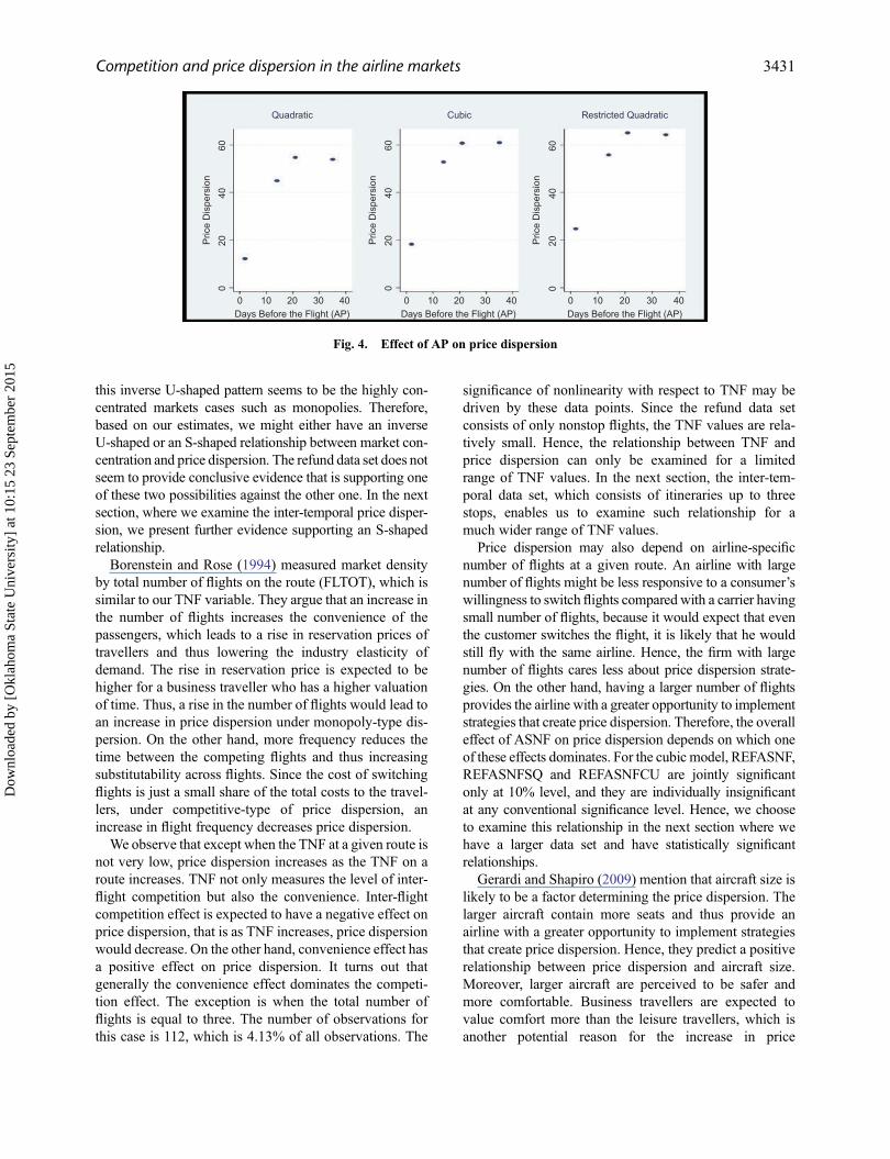
Figure 4 illustrates the link between time of purchaseand price dispersion because of refundable tickets. As it isapparent from the figure, as the flight date approaches, theprice dispersion due to refundable tickets decreases. Thiscan be attributed to the fact that as the flight dateapproaches, the uncertainty decreases, and so the travel-lers would be willing to pay less for a refundable ticket.

Price dispersion by inter-temporal pricing

The inter-temporal data set is much larger than the refunddata set. Moreover, the variation in the variables of inter-temporal data set is higher compared to the refund data set.Hence, we can examine the factors determining pricedispersion more precisely. For this purpose, we estimatethree models: linear, quadratic and cubic. The models forthe inter-temporal data set and estimates are presented inTable 5. The F test rejects linear and quadratic modelagainst the cubic model at 0.001 significance level.14 Inwhat follows, unless otherwise is stated, we will use the

Table 5. Estimates for inter-temporal price dispersion

Model 1: Linear Model 2: Quadratic Model 3: Cubic

PDI Coeff. SE Coeff. SE Coeff. SE

HHI −0.05563 (0.02063)** −0.23776 (0.08683)** 1.95530 (0.30484)***TNF 0.01211 (0.00291)*** −0.07850 (0.00942)*** 0.02406 (0.02324)ASNF −0.11484 (0.00445)*** −0.13035 (0.01443)*** −0.41205 (0.03620)***SIZE 0.07764 (0.00466)*** 0.22844 (0.01933)*** 0.08873 (0.05843)DIST 0.14726 (0.02254)*** 0.18853 (0.02300)*** 0.19368 (0.02301)***DISTSQ −0.02134 (0.00741)** −0.03028 (0.00750)*** −0.03269 (0.00753)***SOLDALL −0.21989 (0.01222)*** −0.21867 (0.01224)*** −0.21234 (0.01224)***DISTSOLDALL −0.02994 (0.00878)*** −0.02761 (0.00880)** −0.02966 (0.00880)***DUR −0.04648 (0.00815)*** −0.04586 (0.00814)*** −0.04513 (0.00813)***DURSQ 0.00091 (0.00049)+ 0.00082 (0.00049)+ 0.00079 (0.00049)HUB −0.02173 (0.01318)+ −0.00356 (0.01333) −0.00547 (0.01345)STOP1 −0.01564 (0.02062) −0.01146 (0.02062) −0.01520 (0.02056)STOP2 0.03203 (0.02202) 0.04110 (0.02204)+ 0.03451 (0.02199)STOP3 0.15122 (0.04203)*** 0.13456 (0.04219)** 0.14043 (0.04206)***POP −0.08472 (0.02918)** −0.17058 (0.02976)*** −0.16594 (0.02987)***PCI 0.00195 (0.00087)* 0.00021 (0.00087) 0.00054 (0.00088)POPPCI 0.00267 (0.00095)** 0.00531 (0.00097)*** 0.00528 (0.00097)***AMPEAK 0.02108 (0.00597)*** 0.01997 (0.00597)*** 0.01897 (0.00596)**PMPEAK −0.10207 (0.01088)*** −0.10282 (0.01089)*** −0.10370 (0.01087)***TEMP 0.00196 (0.00031)*** 0.00164 (0.00031)*** 0.00191 (0.00032)***BIGCITY 0.05591 (0.01100)*** 0.03208 (0.01121)** 0.03945 (0.01125)***DIFFGAMBLE 0.00068 (0.00006)*** 0.00058 (0.00006)*** 0.00066 (0.00006)***LCC 0.07820 (0.00539)*** 0.08427 (0.00551)*** 0.09745 (0.00560)***

(continued )

13 In the refund data, among 22 routes that we examine, 16 of them are long route (i.e. distance is more than 500 miles).14Adjusted R2 agrees with this conclusion.

3432 D. Chakrabarty and L. Kutlu

Dow

nloa

ded

by [

Okl

ahom

a St

ate

Uni

vers

ity]

at 1

0:15

23

Sept

embe

r 20

15

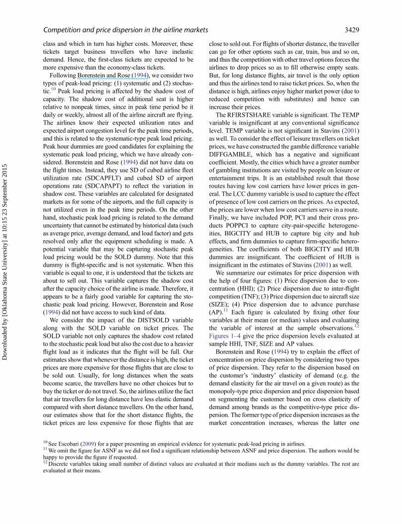
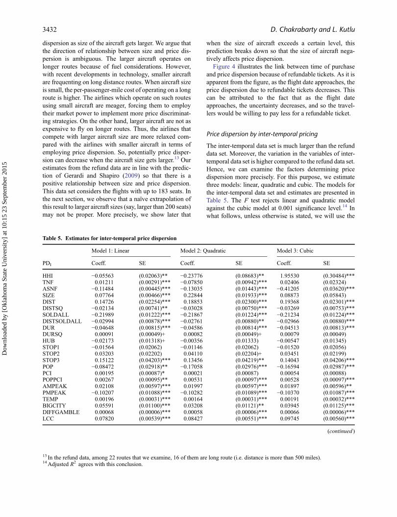
cubic model in our arguments. Figures 5–8 give the pricedispersion levels (measured by PDI = PMAX/PMIN) eval-uated at sample HHI, TNF, ANSF and SIZE values.

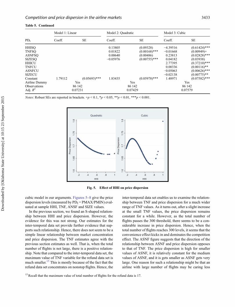
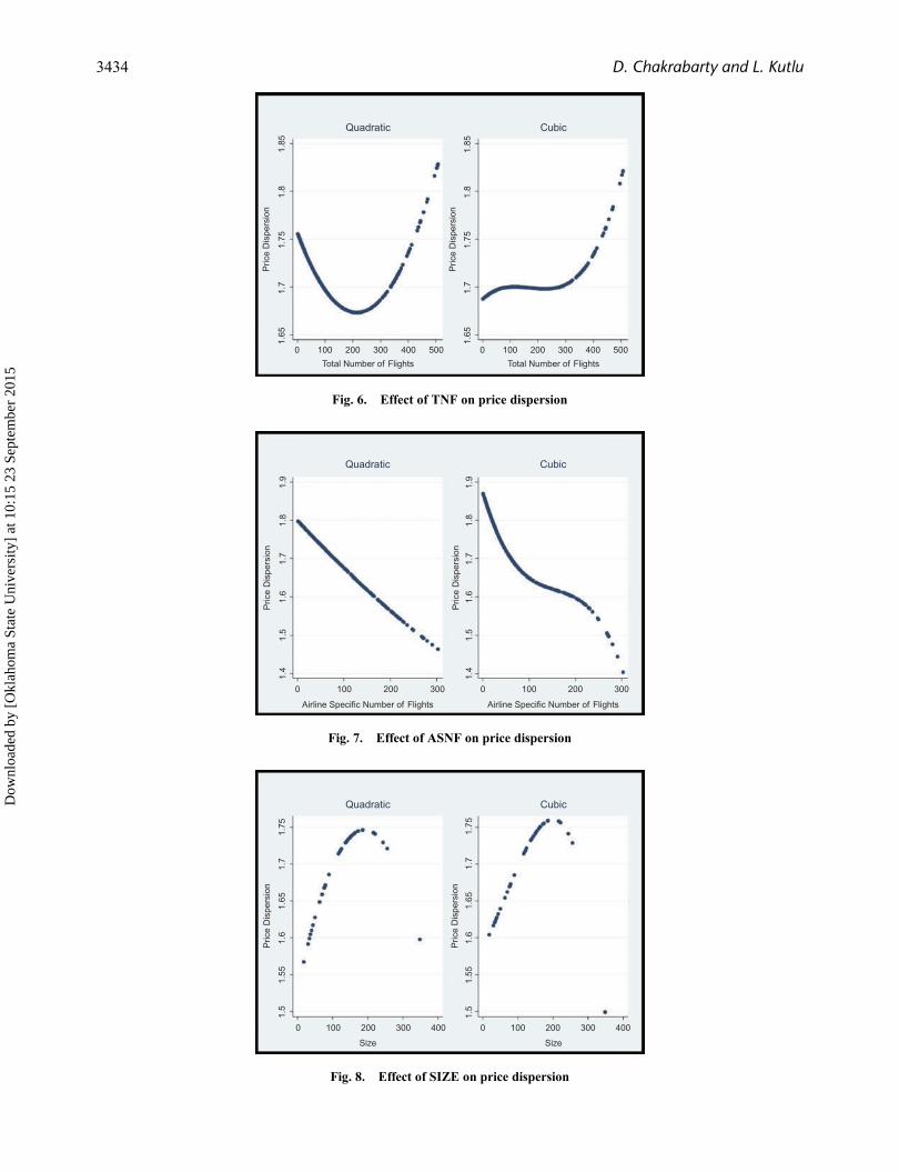
In the previous section, we found an S-shaped relation-ship between HHI and price dispersion. However, theevidence for this was not strong. Our estimates for theinter-temporal data set provide further evidence that sup-ports such relationship. Hence, there does not seem to be asimple linear relationship between market concentrationand price dispersion. The TNF estimates agree with theprevious section estimates as well. That is, when the totalnumber of flights is not large, there is a positive relation-ship. Note that compared to the inter-temporal data set, themaximum value of TNF variable for the refund data set ismuch smaller.15 This is mostly because of the fact that therefund data set concentrates on nonstop flights. Hence, the

inter-temporal data set enables us to examine the relation-ship between TNF and price dispersion for a much widerrange of TNF values. As it turns out, after a slight increaseat the small TNF values, the price dispersion remainsconstant for a while. However, as the total number offlights passes the 300 threshold, there seems to be a con-siderable increase in price dispersion. Hence, when thetotal number of flights reaches 300 levels, it seems that theconvenience effect kicks in and dominates the competitioneffect. The ASNF figure suggests that the direction of therelationship between ASNF and price dispersion opposesto that of TNF. The price dispersion is high for smallervalues of ASNF, it is relatively constant for the mediumvalues of ASNF, and it is gets smaller as ASNF gets verylarge. One reason for such a relationship might be that anairline with large number of flights may be caring less

Table 5. Continued

Model 1: Linear Model 2: Quadratic Model 3: Cubic

PDI Coeff. SE Coeff. SE Coeff. SE

HHISQ 0.13805 (0.09328) −4.39516 (0.61424)***TNFSQ 0.01822 (0.00168)*** −0.01668 (0.00949)+ASNFSQ 0.00640 (0.00486) 0.23813 (0.02828)***SIZESQ −0.05976 (0.00755)*** 0.04182 (0.03938)HHICU 2.77395 (0.37210)***TNFCU 0.00336 (0.00116)**ASNFCU −0.05063 (0.00626)***SIZECU −0.02138 (0.00775)**Constant 1.79112 (0.05693)*** 1.83435 (0.05978)*** 1.48971 (0.07582)***Airline Dummy Yes Yes YesObservations 86 142 86 142 86 142Adj. R2 0.07231 0.07429 0.07579

Notes: Robust SEs are reported in brackets. +p < 0.1, *p < 0.05, **p < 0.01, ***p < 0.001.

1.8

1.75

1.7

Pric

e D

ispe

rsio

n

1.65

.2 .4

Quadratic Cubic

.6

HHI

.8 1 .2 .4 .6

HHI

.8 1

1.6

1.8

1.75

1.7

Pric

e D

ispe

rsio

n

1.65

1.6

Fig. 5. Effect of HHI on price dispersion

15Recall that the maximum value of total number of flights for the refund data is 17.

Competition and price dispersion in the airline markets 3433

Dow

nloa

ded

by [

Okl

ahom

a St

ate

Uni

vers

ity]

at 1

0:15

23

Sept

embe

r 20

15

1.85

1.8

1.75

Pric

e D

ispe

rsio

n

1.7

1.65

1.85

1.8

1.75

Pric

e D

ispe

rsio

n

1.7

1.65

0 100 200 300

Total Number of Flights

Quadratic Cubic

400 500 0 100 200 300

Total Number of Flights

400 500

Fig. 6. Effect of TNF on price dispersion

1.9

1.8

1.7

1.6

Pric

e D

ispe

rsio

n

1.5

1.4

1.9

1.8

1.7

1.6

Pric

e D

ispe

rsio

n

1.5

1.4

0 100 200

Quadratic Cubic

300 0 100 200

Airline Specific Number of FlightsAirline Specific Number of Flights

300

Fig. 7. Effect of ASNF on price dispersion

1.75

1.7

1.65

1.6

Pric

e D

ispe

rsio

n

1.55

1.5

1.75

1.7

1.65

1.6

Pric

e D

ispe

rsio

n

1.55

1.5

0 100 200

Quadratic Cubic

300 400

Size

0 100 200 300 400

Size

Fig. 8. Effect of SIZE on price dispersion

3434 D. Chakrabarty and L. Kutlu

Dow

nloa

ded

by [

Okl

ahom

a St

ate

Uni

vers

ity]

at 1

0:15

23

Sept

embe

r 20

15

about price discrimination strategies. Finally, our esti-mates for SIZE agree with the former section estimatesagain. That is, the refund data set estimates a positiverelationship between SIZE and price dispersion.However, the maximum value of SIZE variable in thatdata set is 183. The inter-temporal data set covers a widerrange of values for the SIZE variable. As it turns out, oncethe number of seats reaches 200, we observe a slightdecrease in price dispersion.16 Therefore, for two differentmeasures of price dispersion and different data sets, ourconclusions about the relationships mostly agree. Thelinearity assumption seems to be strong, and higher orderapproximations are needed to evaluate the relationshipbetween price dispersion of competition.

IV. Conclusion

We examined the relationship between price dispersionand some of the factors that affect it. Unlike most studies,we allowed a nonlinear relationship between price disper-sion and these factors. This enabled us to capture thepotentially nonmonotonic relationships between price dis-persion and these factors. When the relationship betweenthese variables and the price dispersion is U-shaped,inverse U-shaped or S-shaped and we force a linear rela-tionship, it is possible to observe a zero overall effect sothat the estimate for that particular variable is insignificant.This can be a potential reason for mixture of results in theliterature.

One important factor for price dispersion is competi-tion. We considered three forms of competition: inter-firm (measured by HHI), inter-flight (measured by TNF)and frequency (measured by ASNF) competitions. Thetotal number of flights in a route measures also conve-nience. Hence, the overall effect of this variable on pricedispersion is ambiguous. It turned out that, when the totalnumber of flights is large (more than 300), the conveni-ence effect dominates the competition effect. Otherwise,there does not seem to be a strong connection betweentotal number of flights and price dispersion. After con-trolling for inter-flight competition (and other factors),the net effect of market concentration (HHI) on pricedispersion is S-shaped. For the low and high extremesof market concentration, there seems to be a positiverelationship, but for the medium values the relationshipis negative.

An interesting finding was that when the size of aircraftis larger than a certain level, the positive relationshipbetween price dispersion and aircraft size breaks downand becomes negative. This contrasts with the earlierstudies that conjecture a positive relationship between

price dispersion and size of aircraft. We believe that apotential explanation is that for longer routes; airlinesusing smaller aircraft are disadvantageous comparedwith airlines using larger aircraft. Therefore, they feelcompelled to use their price dispersion abilities to thebest extent so as to compensate their disadvantage.Hence, we stress out the importance of considering thenonlinear relationships in price dispersion modelling.

Acknowledgements

We thank Liza Kukharenko and Zhi Qu for their contribu-tions for data collection. The usual caveat applies.

References

Borenstein, S. and Rose, N. L. (1994) Competition and pricedispersion in the U.S. airline industry, Journal of PoliticalEconomy, 102, 653–83. doi:10.1086/261950.

Bresnahan, T. F. (1989) Empirical studies of industries withmarket power, in Handbook of Industrial Organization,Schmalensee, R. and Willig, R. D. (Eds), Vol. 2,North-Holland, Amsterdam, pp. 1011–57.

Dai, M., Liu, Q. and Serfes, K. (2014) Is the effect of competitionon price dispersion non-monotonic? Evidence from the U.S. airline industry, Review of Economics and Statistics, 96,161–70. doi:10.1162/REST_a_00362.

Dana Jr., J. D. (1998) Advance-purchase discounts and pricediscrimination in competitive markets, Journal of PoliticalEconomy, 106, 395–422. doi:10.1086/250014.

Deneckere, R. and Peck, J. (2012) Dynamic competition withrandom demand and costless search: a theory of price post-ing, Econometrica, 80, 1185–247. doi:10.3982/ECTA8806.

Escobari, D. F. (2009) Systematic peak-load pricing, congestionpremia and demand diverting: empirical evidence,Economics Letters, 103, 59–61. doi:10.1016/j.econlet.2009.01.019.

Escobari, D. F. (2012) Dynamic pricing, advance sales, andaggregate demand learning in airlines, The Journal ofIndustrial Economics, 60, 697–724. doi:10.1111/joie.12004.

Escobari, D. F. and Lee, S. Y. (2012) Demand shifting acrossflights and airports in a spatial competition model, Letters inSpatial and Resource Sciences, 5, 175–83. doi:10.1007/s12076-012-0081-4.

Gaggero, A. A. and Piga, C. A. (2011) Airline market powerand intertemporal price dispersion, The Journal ofIndustrial Economics, 59, 552–77. doi:10.1111/j.1467-6451.2011.00467.x

Gale, I. L. and Holmes, T. J. (1993) Advance-purchase discountsand monopoly allocation of capacity, American EconomicReview, 83, 135–46.

Gerardi, K. S. and Shapiro, A. H. (2009) Does competitionreduce price dispersion? New evidence from the airlineindustry, Journal of Political Economy, 117, 1–37.doi:10.1086/597328

Giaume, S. and Guillou, S. (2004) Price discrimination andconcentration in European airline markets, Journal of Air

16We also tried a fourth order polynomial approximation for the SIZE variable. This result was robust to that specification as well.

Competition and price dispersion in the airline markets 3435

Dow

nloa

ded

by [

Okl

ahom

a St

ate

Uni

vers

ity]

at 1

0:15

23

Sept

embe

r 20

15

Transport Management, 10, 305–10. doi:10.1016/j.jairtraman.2004.04.002.

Gillen, D. and Hazledine, T. (2012) Chapter 3 The newpricing in North American air travel markets: implica-tions for competition and antitrust, in Pricing Behaviorand Non-Price Characteristics in the Airline Industry(Advances in Airline Economics, Volume 3), Peoples, J.(Ed), Emerald Group Publishing, Bingley, pp. 55–82.doi:10.1108/S2212-1609(2011)0000003005.

Graham, D. R., Kaplan, D. P. and Sibley, D. S. (1983) Efficiencyand competition in the airline industry, The Bell Journal ofEconomics, 14, 118–38. doi:10.2307/3003541.

Hazledine, T. (2006) Price discrimination in Cournot-Nash oli-gopoly, Economics Letters, 93, 413–20. doi:10.1016/j.econlet.2006.06.006.

Hazledine, T. (2010) Oligopoly price discrimination with manyprices, Economics Letters, 109, 150–53. doi:10.1016/j.econlet.2010.09.009.

Hazledine, T. (2011) Price discrimination in Australasian airtravel markets, New Zealand Economic Papers, 45,311–24. doi:10.1080/00779954.2011.606600.

Kumar, R. and Kutlu, L. (2014) Price Discrimination in QuantitySetting Oligopoly, Unpublished Manuscript.

Kutlu, L. (2009) Price discrimination in Stackelberg competi-tion, The Journal of Industrial Economics, 57, 364.doi:10.1111/j.1467-6451.2009.00382.x

Kutlu, L. (2012) Price discrimination in Cournot competition,Economics Letters, 117, 540–43. doi:10.1016/j.econlet.2012.07.019.

Kutlu, L. and Sickles, R. C. (2012) Estimation of market powerin the presence of firm level inefficiencies, Journal ofEconometrics, 168, 141–55. doi:10.1016/j.jeconom.2011.11.001.

Kutlu, L. and Wang, R. (2014) Price Dispersion, Competition,and Efficiency in the US Airline Industry, UnpublishedManuscript.

Perloff, J. M., Karp, L. S. and Golan, A. (2007) EstimatingMarket Power and Strategies, Cambridge UniversityPress, Cambridge.

Roos, N. D., Mills, G. and Whelan, S. (2010) Pricing dynamicsin the Australian airline market, Economic Record, 86,545–62. doi:10.1111/j.1475-4932.2010.00653.x.

Stavins, J. (2001) Price discrimination in the airline market: theeffect of market concentration, Review of Economicsand Statistics, 83, 200–02. doi:10.1162/rest.2001.83.1.200.

3436 D. Chakrabarty and L. Kutlu

Dow

nloa

ded

by [

Okl

ahom

a St

ate

Uni

vers

ity]

at 1

0:15

23

Sept

embe

r 20

15