artificial binary data scenarios
TRANSCRIPT

Artificial Binary Data Scenarios
Sara DolnicarFriedrich Leisch
Andreas Weingessel
Working Paper No. 20September 1998

September 1998
SFB‘Adaptive Information Systems and Modelling in Economics and Management
Science’
Vienna University of Economicsand Business Administration
Augasse 2–6, 1090 Wien, Austria
in cooperation withUniversity of Vienna
Vienna University of Technology
http://www.wu-wien.ac.at/am
This piece of research was supported by the Austrian Science Foundation(FWF) under grant SFB#010 (‘Adaptive Information Systems and Modelling in
Economics and Management Science’).

Arti�cial Binary Data Scenarios
Sara Dolnicar� Friedrich Leischy Andreas Weingessely
1 Introduction
In order to evaluate the performance of di�erent algorithms for data segmentation data setshave to be used, where the \correct" solution is known in advance. Since for real-world datasets the data generating process is not known, arti�cial data with a prede�ned structure haveto be generated.
In Dolnicar et al. (1998b) various arti�cial data scenarios based on experience with empiricaldata sets have been de�ned. They were used to compare the performance of several \classical"cluster algorithms. In Dolnicar et al. (1998a) some new cluster algorithms have been appliedto these data.
In this manual we describe the data sets used in these experiments together with some newdata sets which complete the range of provided scenarios. Our goal is to set up a benchmarkset of scenarios with di�erent diÆculties which can be used by members of the SFB and otherresearchers to evaluate their cluster algorithms and compare them with previous results.
The data sets described in this manual are available as packages for R (Splus) and asASCII-�les under http://www.ci.tuwien.ac.at/SFB/. The description of the scenarios (seeSection 4) are written in the R-help format language and can be converted to LATEX (as in thismanual) or html. Algorithms for generating arti�cial data scenarios are described in Leischet al. (1998b).
2 Description of the Scenarios
The basic Scenario 1 consists of 12 binary variables which model answers to questions of aquestionnaire. These questions are grouped in 4 groups of 3 variables. Each group correspondsto one latent variable (which could for example describe the general interest in cultural activitiesduring holidays) which is represented by 3 manifest variables (like interest in museums, theaters,and opera). In the data there are 6 types of 1000 data points each which model di�erent answerbehaviors. Each type has a high probability (0.8) to answer \yes" to the questions of 2 latentvariables and a low probability (0.2) for the 2 other latent variables. This scenario is \easy' inthat sense that no cluster algorithm we considered thus far had diÆculties to �nd the 6 clusterstherein. The basic scenario can be made more diÆcult (and thus more realistic) by varying thefollowing parameters
� Size of the clusters (Scenario 5 & 8)
� Di�erent number of manifest variables per latent variable (Scenario 2)
� Smaller di�erence between the \high" and \low" probabilities (Scenario 3)
�Institut f�ur Tourismus und Freizeitwirtschaft,Wirtschaftsuniversit�atWien, Augasse 2-6, A-1090 Wien, Aus-tria. email: [email protected], http://www.wu-wien.ac.at/inst/tourism/locale.html
yInstitut f�ur Statistik, Wahrscheinlichkeitstheorie und Versicherungsmathematik, Technische Universit�atWien, Wiedner Hauptstra�e 8{10/1071, A-1040 Wien, Austria. email: �[email protected],http://www.ci.tuwien.ac.at
1

� Assymetric distribution of 0's and 1's (Scenario 6 & 7)
Scenario 9 models the observation that in real-world data two common \yes"-answers providemore similarity between two persons than two common \no"-answers (Leisch et al., 1998a).Finally, Scenario 0 is random with no prede�ned structure. This can be used as a test scenariosfor algorithms which predict the number of clusters in a data set.
In all these scenarios each variable has been modeled independently. The dependence be-tween manifest variables belonging to one latent variable is only modeled by the mixture of thedi�erent types. For Scenarios 1-3, 5, & 6 there are also data sets with a high correlation betweenthe variables belonging to one latent variable. Scenario 4 is only generated in the dependentform, it is the same as Scenario 1, but with a di�erent correlation structure. Table 1 gives anoverview over all scenarios and shows whether there is a dependent or independent (or both)version of them.
Name Description indep. dep.Scenario 0 Random Scenario XScenario 1 Basic Scenario X XScenario 2 Unequal Latent Variable Scenario X XScenario 3 Medium Importance Scenario X XScenario 4 Bad Indicator Scenario XScenario 5 Niche Segment Scenario X XScenario 6 Answer Tendencies Scenario X XScenario 7 Asymmetric Scenario XScenario 8 Extreme Segment Size Scenario XScenario 9 Important \Yes" Scenario X
Table 1: The Scenarios
The variable-names in R and the �lenames are of the form scen.x for the independentdata sets and scendep.x for the dependent ones, where x is the number of the scenario. InDolnicar et al. (1998a,b) slightly di�erent names of the scenarios have been used, Table 2 givesthe relation between the old and new names.
Old New1a 11b 53a 33b 6
Table 2: Old/New Scenario Names
3 Results
Tables 4-7 show the results of several cluster algorithms applied to the Scenarios 1-6. Table 3lists these cluster algorithms.
The values given in the table are the number of classes found and the number of thoseclusters which have never been found in 10 runs. class. rate map. gives the classi�cationrate only computed for the cluster centers which have been found, class. rate all gives theclassi�cation rate in percent of all data. (center-type)2 gives the Euclidean distance from thecenter to the speci�ed mean values and comp. range describes the variation of the resulting
2

HCL-ED Hard Competitive Learning, Euclidean DistanceHCL-AD Hard Competitive Learning, Absolute Distancek-means K-MeansNGAS-ED Neural Gas, Euclidean DistanceNGAS-AD Neural Gas, Absolute DistanceSOM Self Organizing MapsTRN Topology Representing NetworkHCL-BD Hard Competitive Learning, Binary Distancest-1 Improved Fixpoint Method, Euclidean Distancest-2 Improved Fixpoint Method, f(:) = k:k1:4
st-3 Improved Fixpoint Method, Absolute Distancest-4 Improved Fixpoint Method, f(:) = ln(cosh(k:k))
Table 3: Cluster Algorithms Used
prototypes. The values are given in the form minimum/average/maximum. More details aboutthe algorithms and a discussion of the results can be found in Dolnicar et al. (1998a,b).
4 The Scenarios
In the following we give a description of all the scenarios we have generated thus far. Aftera general description of the scenario, we give two empirical examples, where the structure ofthis scenario could be found in a real-world data set. In a summary section we give some basicdescription as the number of cases, the number of variables and how the manifest variablescorrespond to the latent variables, and the number of classes (=clusters) the scenario is madeof. The Bayes classi�cation rate is the optimal classi�cation rate for the corresponding datagenerating process under the assumption that the class structure is known. It serves as ameasure for the diÆculty of a scenario, see Dolnicar et al. (1998b) for details. The SectionClass Distributions gives the sizes of the classes. Finally, we give a table for the probabilitiesthat a certain variable is 1. For the independent data sets these are the probabilities of the datagenerating process, for the dependent data sets these are, due to computational reasons, themean values of the generated data. The variables are named LxIy, where x gives the numberof the latent variable and y gives the number of the manifest variable for the particular latentvariable.
3

scen.0 Scenario 0: Random Scenario
Description
The Random Scenario is not the result of modeling empirical data. The segment member-ships of the respondents (cases) are determined at random.
Data generation: no correlations between variables modeled (see Working Paper # 7 fordetails)
Summary
Type of variables: binaryNumber of cases: 6000Number of variables: 12Number of classes: 6Number of latent variables: 1Manifest variables per latent variable: 12Bayes classi�cation rate:
Class Distribution
Class Nr.: 1 2 3 4 5 6Number of cases: 1000 1000 1000 1000 1000 1000
Types
(mean values of data generating distribution)
L1I1 L1I2 L1I3 L1I4 L1I5 L1I6 L1I7 L1I8 L1I9 L1I10 L1I11 L1I121 0.5 0.5 0.5 0.5 0.5 0.5 0.5 0.5 0.5 0.5 0.5 0.52 0.5 0.5 0.5 0.5 0.5 0.5 0.5 0.5 0.5 0.5 0.5 0.53 0.5 0.5 0.5 0.5 0.5 0.5 0.5 0.5 0.5 0.5 0.5 0.54 0.5 0.5 0.5 0.5 0.5 0.5 0.5 0.5 0.5 0.5 0.5 0.55 0.5 0.5 0.5 0.5 0.5 0.5 0.5 0.5 0.5 0.5 0.5 0.56 0.5 0.5 0.5 0.5 0.5 0.5 0.5 0.5 0.5 0.5 0.5 0.5
4

scen.1 Scenario 1: Basic Scenario
Description
The basic scenario is not based on typical experiences from empirical data sets. It iscompletely symmetric with six di�erent variables above and six below the average value ofthe entire data set. Furthermore the same amount of individuals (cases) is generated ineach segment.
Data generation: no correlations between variables modeled (see Working Paper # 7 fordetails)
Empirical Examples
Marketing research example
In a survey among buyers of transistor radios 6000 customers or potential customers werequestioned about how important certain features are to them (e.g. technical features, color,size, . . . ). The goal of the study is to identify groups of tourists with the same preferencesthat can be addressed as homogeneous market segments by the marketing management(for product design, product modi�cation, advertising, . . . ). The questionnaire contains 12questions (features of transistor radios). Six segments of travelers with equal segment sizeare known to exist.
Service marketing research example
In a survey among tourists visiting Austria, 6000 travelers were questioned about howimportant certain vacation aspects are to them (e.g. security, comfort, landscape, . . . ). Thegoal of the study is to identify groups of tourists with the same vacation importances /expectations that can be addressed as homogeneous market segments by the destinationmanagement. The questionnaire contains 12 questions (vacation aspects). Six segments oftravelers with equal segment size are known to exist.
Summary
Type of variables: binaryNumber of cases: 6000Number of variables: 12Number of classes: 6Number of latent variables: 4Manifest variables per latent variable: 3-3-3-3Bayes classi�cation rate: 82.98%
Class Distribution
Class Nr.: 1 2 3 4 5 6Number of cases: 1000 1000 1000 1000 1000 1000
Types
(mean values of data generating distribution)
5

L1I1 L1I2 L1I3 L2I1 L2I2 L2I3 L3I1 L3I2 L3I3 L4I1 L4I2 L4I31 0.8 0.8 0.8 0.8 0.8 0.8 0.2 0.2 0.2 0.2 0.2 0.22 0.2 0.2 0.2 0.2 0.2 0.2 0.8 0.8 0.8 0.8 0.8 0.83 0.2 0.2 0.2 0.8 0.8 0.8 0.8 0.8 0.8 0.2 0.2 0.24 0.8 0.8 0.8 0.2 0.2 0.2 0.2 0.2 0.2 0.8 0.8 0.85 0.2 0.2 0.2 0.8 0.8 0.8 0.2 0.2 0.2 0.8 0.8 0.86 0.8 0.8 0.8 0.2 0.2 0.2 0.8 0.8 0.8 0.2 0.2 0.2
6

scendep.1 Scenario 1 (Dependent): Basic Scenario (Dependent)
Description
The basic scenario is not based on typical experiences from empirical data sets. It iscompletely symmetric with six di�erent variables above and below the average value of theentire data set. Furthermore the same amount of individuals (cases) is generated in eachsegment.
Data generation: autologistic model (correlations between variables modeled, see WorkingPaper # 7 for details)
Empirical Examples
Marketing research example
In a survey among buyers of transistor radios 6000 customers or potential customers werequestioned about how important certain features are to them (e.g. technical features, color,size, . . . ). The goal of the study is to identify groups of tourists with the same preferencesthat can be addressed as homogeneous market segments by the marketing management(for product design, product modi�cation, advertising, . . . ). The questionnaire contains12 questions (features of transistor radios), where groups of variables represent a latentdimension and are therefore answered in the same way (e.g. color, size of buttons, designare either all important to an individual or they are not. These variables could all be partof a more complex latent variable called \looks" etc.). Here we suppose that every factoris represented by three questions. These groups of variables are correlated with each other.Six segments of travelers with equal segment size are known to exist.
Service marketing research example
In a survey among tourists visiting Austria, 6000 travelers were questioned about howimportant certain vacation aspects are to them (e.g. security, comfort, landscape, . . . ). Thegoal of the study is to identify groups of tourists with the same vacation importances /expectations that can be addressed as homogeneous market segments by the destinationmanagement. The questionnaire contains 12 questions (vacation aspects), where groups ofvariables represent a latent dimension and are therefore answered in the same way (e.g.the variables landscape, environmental protection, fresh air are either all important to anindividual or they are not. These variables could all be part of a more complex latentvariable called \nature" etc.). Here we suppose that every factor is represented by threequestions. These groups of variables are correlated with each other. Six equally sizedsegments of travelers are known to exist.
Summary
Type of variables: binaryNumber of cases: 6000Number of variables: 12Number of classes: 6Number of latent variables: 4Manifest variables per latent variable: 3-3-3-3Bayes classi�cation rate: 69.52%
7

Class Distribution
Class Nr.: 1 2 3 4 5 6Number of cases: 1000 1000 1000 1000 1000 1000
Types
(mean values of classes)
L1I1 L1I2 L1I3 L2I1 L2I2 L2I3 L3I1 L3I2 L3I3 L4I1 L4I2 L4I31 0.84 0.85 0.86 0.84 0.86 0.86 0.17 0.18 0.20 0.19 0.19 0.202 0.18 0.19 0.18 0.18 0.17 0.18 0.85 0.85 0.86 0.83 0.84 0.853 0.20 0.18 0.19 0.86 0.86 0.86 0.85 0.85 0.85 0.19 0.18 0.194 0.84 0.84 0.85 0.19 0.18 0.18 0.19 0.17 0.19 0.84 0.85 0.845 0.19 0.18 0.18 0.85 0.85 0.86 0.18 0.20 0.20 0.85 0.85 0.876 0.85 0.86 0.85 0.17 0.17 0.17 0.83 0.85 0.84 0.18 0.19 0.20
8

scen.2 Scenario 2: Unequal Latent Variable Scenario
Description
The Unequal Latent Variable Scenario is equivalent to the Basic Scenario as far as symmetryof variables and equality of segment sizes is concerned. As is the case with the Basic Sce-nario, groups of variables represent latent variables (or factors). In the Basis Scenario threevariables represent latent variable indicators. The size of the homogeneous variable groupsranges from �ve variables loading on one latent variable to one single variable representingthe factor in the Unequal Latent Variable Scenario.
Data generation: no correlations between variables modeled (see Working Paper # 7 fordetails)
Empirical Examples
Marketing research example
In a survey among buyers of transistor radios 6000 customers or potential customers werequestioned about how important certain features are to them (e.g. technical features, color,size, . . . ). The goal of the study is to identify groups of tourists with the same preferencesthat can be addressed as homogeneous market segments by the marketing management(for product design, product modi�cation, advertising, . . . ). The questionnaire contains12 questions (features of transistor radios), where groups of variables represent a latentdimension and are therefore answered in the same way (e.g. color, size of buttons, designare either all important to an individual or they are not. These variables could all be partof a more complex latent variable called \looks" etc.). As it is often the case with empiricaldata, some latent variables include more or less actually posed questions. Here we supposethat e.g. factor analysis indicated that �ve questions are caused by the latent variable 1,four by the latent variable 2, two by the latent variable 3 and �nally latent variable 4 is onlyrepresented by one single item of the questionnaire. Six equally sized segments of travelersare known to exist.
Service marketing research example
In a survey among tourists visiting Austria, 6000 travelers were questioned about howimportant certain vacation aspects are to them (e.g. security, comfort, landscape, . . . ). Thegoal of the study is to identify groups of tourists with the same vacation importances /expectations that can be addressed as homogeneous market segments by the destinationmanagement. The questionnaire contains 12 questions (vacation aspects), where groups ofvariables represent a latent dimension and are therefore answered in the same way (e.g.the variables landscape, environmental protection, fresh air are either all important to anindividual or they are not. These variables could all be part of a more complex latentvariable called \nature" etc.). As it is often the case with empirical data, some latentvariables include more or less actually posed questions. Here we suppose that e.g. factoranalysis indicated that �ve questions are caused by the latent variable 1, four by the latentvariable 2, two by the latent variable 3 and �nally latent variable 4 is only represented byone single item of the questionnaire. Six equally sized segments of travelers are known toexist.
9

Summary
Type of variables: binaryNumber of cases: 6000Number of variables: 12Number of classes: 6Number of latent variables: 4Manifest variables per latent variable: 5-4-2-1Bayes classi�cation rate: 82.99%
Class Distribution
Class Nr.: 1 2 3 4 5 6Number of cases: 1000 1000 1000 1000 1000 1000
Types
(mean values of data generating distribution)
L1I1 L1I2 L1I3 L1I4 L1I5 L2I1 L2I2 L2I3 L2I4 L3I1 L3I2 L4I11 0.8 0.8 0.8 0.8 0.8 0.8 0.8 0.8 0.8 0.2 0.2 0.22 0.2 0.2 0.2 0.2 0.2 0.2 0.2 0.2 0.2 0.8 0.8 0.83 0.2 0.2 0.2 0.2 0.2 0.8 0.8 0.8 0.8 0.8 0.8 0.24 0.8 0.8 0.8 0.8 0.8 0.2 0.2 0.2 0.2 0.2 0.2 0.85 0.2 0.2 0.2 0.2 0.2 0.8 0.8 0.8 0.8 0.2 0.2 0.86 0.8 0.8 0.8 0.8 0.8 0.2 0.2 0.2 0.2 0.8 0.8 0.2
10

scendep.2Scenario 2 (Dependent): Unequal Latent Variable Scenario (De-pendent)
Description
The Unequal Latent Variable Scenario is equivalent to the Basic Scenario as far as symmetryof variables and equality of segment sizes is concerned. As is the case with the Basic Sce-nario, groups of variables represent latent variables (or factors). In the Basis Scenario threevariables represent latent variable indicators. The size of the homogeneous variable groupsranges from �ve variables loading on one latent variable to one single variable representingthe factor in the Unequal Latent Variable Scenario.
Data generation: autologistic model (correlations between variables modeled, see WorkingPaper # 7 for details)
Empirical Examples
Marketing research example
In a survey among buyers of transistor radios 6000 customers or potential customers werequestioned about how important certain features are to them (e.g. technical features, color,size, . . . ). The goal of the study is to identify groups of tourists with the same preferencesthat can be addressed as homogeneous market segments by the marketing management(for product design, product modi�cation, advertising, . . . ). The questionnaire contains12 questions (features of transistor radios), where groups of variables represent a latentdimension and are therefore answered in the same way (e.g. color, size of buttons, designare either all important to an individual or they are not. These variables could all be part ofa more complex latent variable called \looks" etc.). These groups of variables are correlatedwith each other. As it is often the case with empirical data, some latent variables includemore or less actually posed questions. Here we suppose that e.g. factor analysis indicatedthat �ve questions are caused by the latent variable 1, four by the latent variable 2, two bythe latent variable 3 and �nally latent variable 4 is only represented by one single item ofthe questionnaire. Six segments of travelers with equal segment size are known to exist.
Service marketing research example
In a survey among tourists visiting Austria, 6000 travelers were questioned about howimportant certain vacation aspects are to them (e.g. security, comfort, landscape, . . . ). Thegoal of the study is to identify groups of tourists with the same vacation importances /expectations that can be addressed as homogeneous market segments by the destinationmanagement. The questionnaire contains 12 questions (vacation aspects), where groups ofvariables represent a latent dimension and are therefore answered in the same way (e.g.the variables landscape, environmental protection, fresh air are either all important to anindividual or they are not. These variables could all be part of a more complex latentvariable called \nature" etc.). These groups of variables are correlated with each other. Asit is often the case with empirical data, some latent variables include more or less actuallyposed questions. Here we suppose that e.g. factor analysis indicated that �ve questions arecaused by the latent variable 1, four by the latent variable 2, two by the latent variable 3and �nally latent variable 4 is only represented by one single item of the questionnaire. Sixequally sized segments of travelers are known to exist.
11

Summary
Type of variables: binaryNumber of cases: 6000Number of variables: 12Number of classes: 6Number of latent variables: 4Manifest variables per latent variable: 5-4-2-1Bayes classi�cation rate: 69.88%
Class Distribution
Class Nr.: 1 2 3 4 5 6Number of cases: 1000 1000 1000 1000 1000 1000
Types
(mean values of classes)
L1I1 L1I2 L1I3 L1I4 L1I5 L2I1 L2I2 L2I3 L2I4 L3I1 L3I2 L4I11 0.86 0.85 0.84 0.83 0.81 0.84 0.87 0.87 0.87 0.17 0.18 0.162 0.20 0.18 0.18 0.15 0.12 0.11 0.13 0.16 0.16 0.81 0.82 0.813 0.21 0.19 0.19 0.17 0.12 0.83 0.85 0.85 0.86 0.81 0.82 0.164 0.87 0.87 0.84 0.84 0.82 0.10 0.15 0.16 0.16 0.16 0.16 0.835 0.21 0.18 0.18 0.17 0.12 0.83 0.87 0.87 0.87 0.18 0.17 0.856 0.85 0.86 0.85 0.83 0.81 0.10 0.12 0.14 0.17 0.82 0.84 0.16
12

scen.3 Scenario 3: Medium Importance Scenario
Description
The Medium Importance Scenario certainly comes closest to what reality is all about. Notgiving up symmetry and equal segment size (Basic Scenario), the restriction of variablesto either below or above average answers is abandoned. Each segment rates six (di�erent)variables higher then the average (of the entire data), but the remaining variables do notaid the distinction by being far below average.
Data generation: no correlations between variables modeled (see Working Paper # 7 fordetails)
Empirical Examples
Marketing research example
In a survey among buyers of transistor radios 6000 customers or potential customers werequestioned about how important certain features are to them (e.g. technical features, color,size, . . . ). The goal of the study is to identify groups of tourists with the same preferencesthat can be addressed as homogeneous market segments by the marketing management(for product design, product modi�cation, advertising, . . . ). The questionnaire contains12 questions (features of transistor radios). Six segments of travelers with equal segmentsize are known to exist, with each group attaching more than average importance to 6features, while attaching medium importance to the remaining attributes of transistor radios(as opposed to low importance statements in the Basic Scenario). Analysis might show(to produce some prejudice here), that heavy metal listeners do have some expectationsabout all features, but only the technical attributes like loudness and possibility to adjustthe bass level are crucial to them. This assumption is more realistic than believing thatevery respondent answers in an extreme manner (don't care at all/ very important) to allattributes listed.
Service marketing research example
In a survey among tourists visiting Austria, 6000 travelers were questioned about howimportant certain vacation aspects are to them (e.g. security, comfort, landscape, . . . ). Thegoal of the study is to identify groups of tourists with the same vacation importances /expectations that can be addressed as homogeneous market segments by the destinationmanagement. The questionnaire contains 12 questions (vacation aspects). Six segments oftravelers with equal segment size are known to exist, with each group attaching more thanaverage importance to 6 questions, while attaching medium importance to the remainingtravel aspects (as opposed to low importance statements in the Basic Scenario). For examplethe result of analysis could be, that culture tourists do not attach very high importanceto comfort and relaxation, but cultural o�ers and interesting sights are crucial variablesseen as extremely important for their stay in Austria. This assumption is more realisticthan believing that every respondent answers in an extreme manner (don't care at all/ veryimportant) to all vacation aspects listed.
13

Summary
Type of variables: binaryNumber of cases: 6000Number of variables: 12Number of classes: 6Number of latent variables: 4Manifest variables per latent variable: 3-3-3-3Bayes classi�cation rate: 48.93%
Class Distribution
Class Nr.: 1 2 3 4 5 6Number of cases: 1000 1000 1000 1000 1000 1000
Types
(mean values of data generating distribution)
L1I1 L1I2 L1I3 L2I1 L2I2 L2I3 L3I1 L3I2 L3I3 L4I1 L4I2 L4I31 0.8 0.8 0.8 0.8 0.8 0.8 0.5 0.5 0.5 0.5 0.5 0.52 0.5 0.5 0.5 0.5 0.5 0.5 0.8 0.8 0.8 0.8 0.8 0.83 0.5 0.5 0.5 0.8 0.8 0.8 0.8 0.8 0.8 0.5 0.5 0.54 0.8 0.8 0.8 0.5 0.5 0.5 0.5 0.5 0.5 0.8 0.8 0.85 0.5 0.5 0.5 0.8 0.8 0.8 0.5 0.5 0.5 0.8 0.8 0.86 0.8 0.8 0.8 0.5 0.5 0.5 0.8 0.8 0.8 0.5 0.5 0.5
14

scendep.3Scenario 3 (Dependent): Medium Importance Scenario (Depen-dent)
Description
The Medium Importance Scenario certainly comes closest to what reality is all about. Notgiving up symmetry and equal segment size (Basic Scenario), the restriction of variablesto either below or above average answers is abandoned. Each segment rates six (di�erent)variables higher then the average (of the entire data), but the remaining variables do notaid the distinction with far below-average values.
Data generation: autologistic model (correlations between variables modeled, see WorkingPaper # 7 for details)
Empirical Examples
Marketing research example
In a survey among buyers of transistor radios 6000 customers or potential customers werequestioned about how important certain features are to them (e.g. technical features, color,size, . . . ). The goal of the study is to identify groups of tourists with the same preferencesthat can be addressed as homogeneous market segments by the marketing management(for product design, product modi�cation, advertising, . . . ). The questionnaire contains12 questions (features of transistor radios), where groups of variables represent a latentdimension and are therefore answered in the same way (e.g. color, size of buttons, designare either all important to an individual or they are not. These variables could all be partof a more complex latent variable called \looks" etc.). Here we suppose that every factor isrepresented by three questions. These groups of variables are correlated with each other. Sixsegments of travelers with equal segment size are known to exist, with each group attachingmore than average importance to 6 questions, while attaching medium importance to theremaining transistor radio attributes (as opposed to low importance statements in the BasicScenario).
Service marketing research example
In a survey among tourists visiting Austria, 6000 travelers were questioned about howimportant certain vacation aspects are to them (e.g. security, comfort, landscape, . . . ). Thegoal of the study is to identify groups of tourists with the same vacation importances /expectations that can be addressed as homogeneous market segments by the destinationmanagement. The questionnaire contains 12 questions (vacation aspects), where groups ofvariables represent a latent dimension and are therefore answered in the same way (e.g.the variables landscape, environmental protection, fresh air are either all important to anindividual or they are not. These variables could all be part of a more complex latentvariable called \nature" etc.). Here we suppose that every factor is represented by threequestions. These groups of variables are correlated with each other. Six equally sizedsegments of travelers are known to exist, with each group attaching more than averageimportance to 6 questions, while attaching medium importance to the remaining travelaspects (as opposed to low importance statements in the Basic Scenario).
15

Summary
Type of variables: binaryNumber of cases: 6000Number of variables: 12Number of classes: 6Number of latent variables: 4Manifest variables per latent variable: 3-3-3-3Bayes classi�cation rate: 41.87%
Class Distribution
Class Nr.: 1 2 3 4 5 6Number of cases: 1000 1000 1000 1000 1000 1000
Types
(mean values of classes)
L1I1 L1I2 L1I3 L2I1 L2I2 L2I3 L3I1 L3I2 L3I3 L4I1 L4I2 L4I31 0.82 0.82 0.83 0.84 0.83 0.83 0.46 0.48 0.51 0.49 0.50 0.512 0.51 0.50 0.52 0.48 0.49 0.50 0.84 0.85 0.85 0.84 0.83 0.833 0.47 0.49 0.48 0.84 0.85 0.83 0.84 0.83 0.84 0.47 0.49 0.504 0.84 0.82 0.83 0.46 0.48 0.49 0.49 0.50 0.52 0.85 0.86 0.865 0.50 0.51 0.51 0.83 0.85 0.84 0.48 0.49 0.50 0.83 0.83 0.856 0.85 0.85 0.86 0.49 0.51 0.51 0.83 0.83 0.83 0.46 0.49 0.51
16

scendep.4 Scenario 4 (Dependent): Bad Indicator Scenario (Dependent)
Description
All dependent scenarios model correlation between those variables that result from the samelatent variable. In case of the Bad Indicator Scenario one of the variables within each groupof three is correlated with the remaining couple of items to a lower extent.
Data generation: autologistic model (correlations between variables modeled, see WorkingPaper # 7 for details)
Empirical Examples
Marketing research example
In a survey among buyers of transistor radios 6000 customers or potential customers werequestioned about how important certain features are to them (e.g. technical features, color,size, . . . ). The goal of the study is to identify groups of tourists with the same preferencesthat can be addressed as homogeneous market segments by the marketing management(for product design, product modi�cation, advertising, . . . ). The questionnaire contains12 questions (features of transistor radios), where groups of variables represent a latentdimension and are therefore answered in the same way (e.g. color, size of buttons, designare either all important to an individual or they are not. These variables could all bepart of a more complex latent variable called \looks" etc.). Here we suppose that everyfactor is represented by three questions. These groups of variables are correlated with eachother. But one variable is correlated to a lower extent, indicating that the question doesnot represent the underlying latent variable as well as the remaining two questions do (e.g.color and design better represent the \look of the radio" as the button size does). Sixsegments of travelers with equal segment size are known to exist.
Service marketing research example
In a survey among tourists visiting Austria, 6000 travelers were questioned about howimportant certain vacation aspects are to them (e.g. security, comfort, landscape, . . . ). Thegoal of the study is to identify groups of tourists with the same vacation importances /expectations that can be addressed as homogeneous market segments by the destinationmanagement. The questionnaire contains 12 questions (vacation aspects), where groups ofvariables represent a latent dimension and are therefore answered in the same way (e.g.the variables landscape, environmental protection, fresh air are either all important to anindividual or they are not. These variables could all be part of a more complex latentvariable called \nature" etc.). Here we suppose that every factor is represented by threequestions. These groups of variables are correlated with each other. But one variable iscorrelated to a lower extent, indicating that the question does not represent the underlyinglatent variable as well as the remaining two questions do (e.g. fresh air and landscapebetter represent \nature" as environmental protection does). Six equally sized segments oftravelers are known to exist.
17

Summary
Type of variables: binaryNumber of cases: 6000Number of variables: 12Number of classes: 6Number of latent variables: 4Manifest variables per latent variable: 3-3-3-3Bayes classi�cation rate: 81.2%
Class Distribution
Class Nr.: 1 2 3 4 5 6Number of cases: 1000 1000 1000 1000 1000 1000
Types
(mean values of classes)
L1I1 L1I2 L1I3 L2I1 L2I2 L2I3 L3I1 L3I2 L3I3 L4I1 L4I2 L4I31 0.84 0.86 0.89 0.83 0.85 0.86 0.19 0.17 0.12 0.20 0.21 0.152 0.17 0.20 0.14 0.18 0.19 0.16 0.86 0.86 0.89 0.85 0.86 0.903 0.16 0.18 0.16 0.84 0.85 0.89 0.84 0.85 0.87 0.19 0.19 0.154 0.85 0.86 0.90 0.19 0.21 0.13 0.16 0.19 0.14 0.84 0.87 0.875 0.18 0.19 0.13 0.84 0.84 0.88 0.18 0.18 0.12 0.85 0.87 0.896 0.84 0.86 0.88 0.19 0.21 0.15 0.86 0.86 0.89 0.20 0.21 0.14
18

scen.5 Scenario 5: Niche Segment Scenario
Description
The symmetry of above and below average variables is the same as for the Basic Scenario:In each segment generated six (di�erent) variables are above / below average. As opposedto the Basic Scenario, the number of individuals (cases) varies over the segments, with thetiny segment number 2 representing a niche.
Data generation: no correlations between variables modeled (see Working Paper # 7 fordetails)
Empirical Examples
Marketing research example
In a survey among buyers of transistor radios 6000 customers or potential customers werequestioned about how important certain features are to them (e.g. technical features, color,size, . . . ). The goal of the study is to identify groups of tourists with the same preferencesthat can be addressed as homogeneous market segments by the marketing management(for product design, product modi�cation, advertising, . . . ). The questionnaire contains 12questions (features of transistor radios). Six segments of travelers are known to exist. Asit is the case in reality, the size of these consumer segments varies.
Service marketing research example
In a survey among tourists visiting Austria, 6000 travelers were questioned about howimportant certain vacation aspects are to them (e.g. security, comfort, landscape, . . . ). Thegoal of the study is to identify groups of tourists with the same vacation importances /expectations that can be addressed as homogeneous market segments by the destinationmanagement. The questionnaire contains 12 questions (vacation aspects). Six segments oftravelers are known to exist. As it is the case in reality, the size of these consumer segmentsvaries.
Summary
Type of variables: binaryNumber of cases: 6000Number of variables: 12Number of classes: 6Number of latent variables: 4Manifest variables per latent variable: 3-3-3-3Bayes classi�cation rate: 88.85%
Class Distribution
Class Nr.: 1 2 3 4 5 6Number of cases: 1000 300 700 3000 500 500
Types
(mean values of data generating distribution)
19

L1I1 L1I2 L1I3 L2I1 L2I2 L2I3 L3I1 L3I2 L3I3 L4I1 L4I2 L4I31 0.8 0.8 0.8 0.8 0.8 0.8 0.2 0.2 0.2 0.2 0.2 0.22 0.2 0.2 0.2 0.2 0.2 0.2 0.8 0.8 0.8 0.8 0.8 0.83 0.2 0.2 0.2 0.8 0.8 0.8 0.8 0.8 0.8 0.2 0.2 0.24 0.8 0.8 0.8 0.2 0.2 0.2 0.2 0.2 0.2 0.8 0.8 0.85 0.2 0.2 0.2 0.8 0.8 0.8 0.2 0.2 0.2 0.8 0.8 0.86 0.8 0.8 0.8 0.2 0.2 0.2 0.8 0.8 0.8 0.2 0.2 0.2
20

scendep.5 Scenario 5 (Dependent): Niche Segment Scenario (Dependent)
Description
The symmetry of above and below average variables is the same as for the Basic Scenario:In each segment generated six (di�erent) variables are above / below average. As opposedto the Basic Scenario, the number of individuals (cases) varies over the segments, with thetiny segment number 2 representing a niche.
Data generation: autologistic model (correlations between variables modeled, see WorkingPaper # 7 for details)
Empirical Examples
Marketing research example
In a survey among buyers of transistor radios 6000 customers or potential customers werequestioned about how important certain features are to them (e.g. technical features, color,size, . . . ). The goal of the study is to identify groups of tourists with the same preferencesthat can be addressed as homogeneous market segments by the marketing management(for product design, product modi�cation, advertising, . . . ). The questionnaire contains12 questions (features of transistor radios), where groups of variables represent a latentdimension and are therefore answered in the same way (e.g. color, size of buttons, designare either all important to an individual or they are not. These variables could all be partof a more complex latent variable called \looks" etc.). Here we suppose that every factoris represented by three questions. These groups of variables are correlated with each other.Six segments of travelers are known to exist. As it is the case in reality, the size of theseconsumer segments varies.
Service marketing research example
In a survey among tourists visiting Austria, 6000 travelers were questioned about how im-portant certain aspects are to them (e.g. security, comfort, landscape, . . . ). The goal of thestudy is to identify groups of tourists with the same vacation importances / expectationsthat can be addressed as homogeneous market segments by the destination management.The questionnaire contains 12 questions (vacation aspects), where groups of variables rep-resent a latent dimension and are therefore answered in the same way (e.g. the variableslandscape, environmental protection, fresh air are either all important to an individual orthey are not. These variables could all be part of a more complex latent variable called\nature" etc.). Here we suppose that every factor is represented by three questions. Thesegroups of variables are correlated with each other. Six segments of travelers are known toexist. As it is the case in reality, the size of these consumer segments varies.
Summary
Type of variables: binaryNumber of cases: 6000Number of variables: 12Number of classes: 6Number of latent variables: 4Manifest variables per latent variable: 3-3-3-3Bayes classi�cation rate: 78.23%
21

Class Distribution
Class Nr.: 1 2 3 4 5 6Number of cases: 1000 300 700 3000 500 500
Types
(mean values of classes)
L1I1 L1I2 L1I3 L2I1 L2I2 L2I3 L3I1 L3I2 L3I3 L4I1 L4I2 L4I31 0.85 0.85 0.87 0.84 0.86 0.86 0.16 0.16 0.16 0.17 0.16 0.152 0.16 0.19 0.19 0.20 0.18 0.22 0.90 0.90 0.91 0.87 0.86 0.853 0.20 0.21 0.20 0.84 0.86 0.85 0.84 0.84 0.85 0.18 0.17 0.194 0.84 0.85 0.85 0.17 0.17 0.18 0.17 0.18 0.17 0.85 0.84 0.855 0.17 0.20 0.18 0.83 0.84 0.84 0.16 0.16 0.17 0.85 0.85 0.866 0.79 0.82 0.81 0.18 0.17 0.20 0.85 0.84 0.86 0.16 0.16 0.14
22

scen.6 Scenario 6: Answer Tendencies Scenario
Description
In reality numerous answer tendencies occur in empirical data sets. That is usually causedby personality traits of the respondents. In the Answer Tendencies Scenario two segmentsare modeled, that basically give the same answer on each one of the 12 questions. Thesymmetry of the Basic Scenario is thus given up, the segment sizes remain equal.
Data generation: no correlations between variables modeled (see Working Paper # 7 fordetails)
Empirical Examples
Marketing research example
In a survey among buyers of transistor radios 6000 customers or potential customers werequestioned about how important certain features are to them (e.g. technical features, color,size, . . . ). The goal of the study is to identify groups of tourists with the same preferencesthat can be addressed as homogeneous market segments by the marketing management(for product design, product modi�cation, advertising, . . . ). The questionnaire contains 12questions (features of transistor radios). Six segments of travelers with equal segment sizeare known to exist. While four segments have a di�erentiated view about the importanceof the attributes of transistor radios stated in the questionnaire, one group of consumersbelieves that not a single one of these attributes is important (imagine buyers who need alittle radio in the kitchen only to listen to the news from time to time when washing thedishes) and another group attaches high importance to each aspect (maybe the group ofmusic enjoyers).
Service marketing research example
Empirical example: In a survey among tourists visiting Austria, 6000 travelers were ques-tioned about how important certain vacation aspects are to them (e.g. security, comfort,landscape, . . . ). The goal of the study is to identify groups of tourists with the same vaca-tion importances / expectations that can be addressed as homogeneous market segments bythe destination management. The questionnaire contains 12 questions (vacation aspects).Six segments of travelers with equal segment size are known to exist. While four segmentshave a di�erentiated view about the importance of the vacation aspects stated in the ques-tionnaire, one tourist group believes, that not a single one of these attributes is important(they might be visiting friends and therefore primarily care about talking with them alot) and another group attaches high importance to each aspect (this could be a group oftourists that does not spend a vacation in a foreign country very often and therefore hasthe highest expectations concerning everything).
Summary
Type of variables: binaryNumber of cases: 6000Number of variables: 12Number of classes: 6Number of latent variables: 4Manifest variables per latent variable: 3-3-3-3Bayes classi�cation rate: 81.25%
23

Class Distribution
Class Nr.: 1 2 3 4 5 6Number of cases: 1000 1000 1000 1000 1000 1000
Types
(mean values of data generating distribution)
L1I1 L1I2 L1I3 L2I1 L2I2 L2I3 L3I1 L3I2 L3I3 L4I1 L4I2 L4I31 0.8 0.8 0.8 0.8 0.8 0.8 0.8 0.8 0.8 0.8 0.8 0.82 0.2 0.2 0.2 0.2 0.2 0.2 0.2 0.2 0.2 0.2 0.2 0.23 0.8 0.8 0.8 0.2 0.2 0.2 0.2 0.2 0.2 0.2 0.2 0.24 0.2 0.2 0.2 0.8 0.8 0.8 0.2 0.2 0.2 0.2 0.2 0.25 0.2 0.2 0.2 0.2 0.2 0.2 0.8 0.8 0.8 0.2 0.2 0.26 0.2 0.2 0.2 0.2 0.2 0.2 0.2 0.2 0.2 0.8 0.8 0.8
24

scendep.6 Scenario 6 (Dependent): Answer Tendencies Scenario (Dependent)
Description
In reality numerous answer tendencies occur in empirical data sets, that is usually causedby personality traits of the respondents. In the Answer Tendencies Scenario two segmentsare modeled, that basically give the same answer on each one of the 12 questions. Thesymmetry of the Basic Scenario id given up, the segment sizes remain equal.
Data generation: autologistic model (correlations between variables modeled, see WorkingPaper # 7 for details)
Empirical Examples
Marketing research example
In a survey among buyers of transistor radios 6000 customers or potential customers werequestioned about how important certain features are to them (e.g. technical features, color,size, . . . ). The goal of the study is to identify groups of tourists with the same preferencesthat can be addressed as homogeneous market segments by the marketing management(for product design, product modi�cation, advertising, . . . ). The questionnaire contains12 questions (features of transistor radios), where groups of variables represent a latentdimension and are therefore answered in the same way (e.g. color, size of buttons, designare either all important to an individual or they are not. These variables could all bepart of a more complex latent variable called \looks" etc.). Here we suppose that everyfactor is represented by three questions. These groups of variables are correlated with eachother. Six segments of travelers with equal segment size are known to exist. While foursegments have a di�erentiated view about the importance of the attributes of transistorradios stated in the questionnaire, one group of consumers believes, that not a single one ofthese attributes is important (imagine buyers who need a little radio in the kitchen only tolisten to the news from time to time when washing the dishes) and another group attacheshigh importance to each aspect (maybe the group of music enjoyers).
Service marketing research example
In a survey among tourists visiting Austria, 6000 travelers were questioned about how im-portant certain aspects are to them (e.g. security, comfort, landscape, . . . ). The goal of thestudy is to identify groups of tourists with the same vacation importances / expectationsthat can be addressed as homogeneous market segments by the destination management.The questionnaire contains 12 questions (vacation aspects), where groups of variables rep-resent a latent dimension and are therefore answered in the same way (e.g. the variableslandscape, environmental protection, fresh air are either all important to an individual orthey are not. These variables could all be part of a more complex latent variable called\nature" etc.). Here we suppose that every factor is represented by three questions. Thesegroups of variables are correlated with each other. Six equally sized segments of travelersare known to exist. While four segments have a di�erentiated view about the importanceof the vacation aspects stated in the questionnaire, one tourist group believes, that nota single one of these attributes is important (they might be visiting friends and thereforeprimarily care about talking with them a lot) and another group attaches high importanceto each aspect (this could be a group of tourists that does not spend a vacation in a foreigncountry very often and therefore has the highest expectations concerning everything).
25

Summary
Type of variables: binaryNumber of cases: 6000Number of variables: 12Number of classes: 6Number of latent variables: 4Manifest variables per latent variable: 3-3-3-3Bayes classi�cation rate: 71.08%
Class Distribution
Class Nr.: 1 2 3 4 5 6Number of cases: 1000 1000 1000 1000 1000 1000
Types
(mean values of classes)
L1I1 L1I2 L1I3 L2I1 L2I2 L2I3 L3I1 L3I2 L3I3 L4I1 L4I2 L4I31 0.80 0.81 0.80 0.92 0.93 0.93 0.83 0.83 0.83 0.79 0.80 0.812 0.06 0.08 0.10 0.16 0.19 0.20 0.07 0.07 0.08 0.06 0.08 0.083 0.82 0.83 0.84 0.18 0.21 0.22 0.18 0.18 0.21 0.18 0.18 0.204 0.16 0.19 0.20 0.92 0.93 0.93 0.18 0.20 0.21 0.17 0.20 0.215 0.19 0.19 0.20 0.20 0.20 0.21 0.83 0.83 0.84 0.18 0.20 0.216 0.19 0.19 0.20 0.17 0.18 0.21 0.17 0.18 0.20 0.81 0.81 0.81
26

scen.7 Scenario 7: Asymmetric Scenario
Description
The Asymmetric Scenario gives up the symmetry restriction of the Basic scenario hangingon to the assumption of the same number of respondent (cases) existing in each segment.
Data generation: no correlations between variables modeled
Empirical Examples
Marketing research example
In a survey among buyers of transistor radios 6000 customers or potential customers werequestioned about how important certain features are to them (e.g. technical features, color,size, . . . ). The goal of the study is to identify groups of tourists with the same preferencesthat can be addressed as homogeneous market segments by the marketing management(for product design, product modi�cation, advertising, . . . ). The questionnaire contains 12questions (features of transistor radios). Segments do not attach great importance to sixand low importance to the remaining six features listed in the questionnaire. Instead, upto nine product attributes are rated important by the di�erent segments. Six segments oftravelers with equal segment size are known to exist.
Service marketing research example
In a survey among tourists visiting Austria, 6000 travelers were questioned about howimportant certain vacation aspects are to them (e.g. security, comfort, landscape, . . . ). Thegoal of the study is to identify groups of tourists with the same vacation importances /expectations that can be addressed as homogeneous market segments by the destinationmanagement. The questionnaire contains 12 questions (vacation aspects). Segments do notattach great importance to six and low importance to the remaining six questions. Instead,up to nine vacation aspects are rated important by the di�erent segments. Six segments oftravelers with equal segment size are known to exist.
Summary
Type of variables: binaryNumber of cases: 6000Number of variables: 12Number of classes: 6Number of latent variables: 4Manifest variables per latent variable: 3-3-3-3Bayes classi�cation rate:
Class Distribution
Class Nr.: 1 2 3 4 5 6Number of cases: 1000 1000 1000 1000 1000 1000
Types
(mean values of data generating distribution)
27

L1I1 L1I2 L1I3 L2I1 L2I2 L2I3 L3I1 L3I2 L3I3 L4I1 L4I2 L4I31 0.8 0.8 0.8 0.8 0.8 0.8 0.2 0.2 0.2 0.2 0.2 0.22 0.2 0.2 0.2 0.8 0.8 0.8 0.8 0.8 0.8 0.8 0.8 0.83 0.2 0.2 0.2 0.8 0.8 0.8 0.8 0.8 0.8 0.2 0.2 0.24 0.8 0.8 0.8 0.2 0.2 0.2 0.2 0.2 0.2 0.8 0.8 0.85 0.2 0.2 0.2 0.2 0.2 0.2 0.2 0.2 0.2 0.8 0.8 0.86 0.8 0.8 0.8 0.2 0.2 0.2 0.8 0.8 0.8 0.8 0.8 0.8
28

scen.8 Scenario 8: Extreme Segment Size Scenario
Description
The Basic Scenario assumes that the same amount of respondents (cases) exists (and isthus generated) in each segment. The Niche Market Scenario gives up this restrictionby de�ning six groups of respondents with di�erent sizes each. In the Extreme SegmentScenario three small consumer groups (with the same size|n=300|as the tiny segment inthe Niche Market Scenario) are de�ned. The remaining three segments are equally sizedlarge segments including 1700 respondents.
Data generation: no correlations between variables modeled
Empirical Examples
Marketing research example
In a survey among buyers of transistor radios 6000 customers or potential customers werequestioned about how important certain features are to them (e.g. technical features, color,size, . . . ). The goal of the study is to identify groups of tourists with the same preferencesthat can be addressed as homogeneous market segments by the marketing management(for product design, product modi�cation, advertising, . . . ). The questionnaire contains12 questions (features of transistor radios). Six segments of travelers with equal segmentsize are known to exist, with three of them representing niche markets (with 300 customerseach) and three representing mass markets (with 1.700 respondents each).
Service marketing research example
In a survey among tourists visiting Austria, 6000 travelers were questioned about howimportant certain vacation aspects are to them (e.g. security, comfort, landscape, . . . ). Thegoal of the study is to identify groups of tourists with the same vacation importances /expectations that can be addressed as homogeneous market segments by the destinationmanagement. The questionnaire contains 12 questions (vacation aspects). Six segmentsof travelers are known to exist, with three of them representing niche markets (with 300customers each) and three representing mass segments (with 1.700 respondents each).
Summary
Type of variables: binaryNumber of cases: 6000Number of variables: 12Number of classes: 6Number of latent variables: 4Manifest variables per latent variable: 3-3-3-3Bayes classi�cation rate:
Class Distribution
Class Nr.: 1 2 3 4 5 6Number of cases: 300 300 300 1700 1700 1700
29
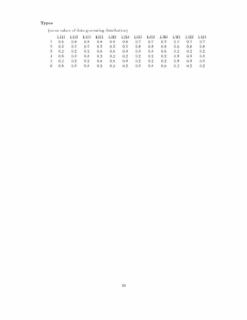
Types
(mean values of data generating distribution)
L1I1 L1I2 L1I3 L2I1 L2I2 L2I3 L3I1 L3I2 L3I3 L4I1 L4I2 L4I31 0.8 0.8 0.8 0.8 0.8 0.8 0.2 0.2 0.2 0.2 0.2 0.22 0.2 0.2 0.2 0.2 0.2 0.2 0.8 0.8 0.8 0.8 0.8 0.83 0.2 0.2 0.2 0.8 0.8 0.8 0.8 0.8 0.8 0.2 0.2 0.24 0.8 0.8 0.8 0.2 0.2 0.2 0.2 0.2 0.2 0.8 0.8 0.85 0.2 0.2 0.2 0.8 0.8 0.8 0.2 0.2 0.2 0.8 0.8 0.86 0.8 0.8 0.8 0.2 0.2 0.2 0.8 0.8 0.8 0.2 0.2 0.2
30

scen.9 Scenario 9: Important \Yes" Scenario
Description
The basic scenario is not based on typical experiences from empirical data sets. It iscompletely symmetric and assumes the same amount of individuals (cases) to be membersof the clusters generated. The Important \Yes" Scenario is more realistic concerning bothrestrictions: the average segment ratings do not have to be high in six variables and low inthe remaining six, the design is thus asymmetric. Also, the segments sizes di�er from eachother.
Data generation: no correlations between variables modeled
Empirical Examples
Marketing research example
In a survey among buyers of tiny portable transistor radios 6000 customers or potentialcustomers were questioned about the usage of these tiny portable radios (e.g. in the car,in the oÆce, at home, . . . ). The goal of the study is to identify groups of tourists withthe kinds of radio usage that can be addressed as homogeneous market segments by themarketing management (for product design, product modi�cation, advertising, . . . ). Thequestionnaire contains 12 questions (features of transistor radios). Six segments of travelerswith equal segment size are known to exist. Of course a large number of respondents willprobably not use these tiny portable transistor radios at all. The positive answers are thusmore informative for the behavioral segmentation desired and a large segment of non-userswill occur.
Service marketing research example
In a survey among tourists visiting Austria, 6000 travelers were questioned about whatvacation activities they engage in (e.g. tennis, jogging, skiing, sightseeing, . . . ). The goalof the study is to identify groups of tourists with the same vacation activities that can beaddressed as homogeneous market segments by the destination management. The ques-tionnaire contains 12 questions (activities). Each segment shows a di�erent pattern ofactivities. The fact, that tourists state an activity is more informative than the statement,not to e.g. play tennis. It is therefore important to identify segments with speci�c activitycombinations then to de�ne them by a lack of certain activities. Six segments of travelerswith di�erent segment size are known to exist, where a large amount of respondents doesnot indicate any activity at all.
Summary
Type of variables: binaryNumber of cases: 4000Number of variables: 10Number of classes: 5Number of latent variables: 4Manifest variables per latent variable: 2-3-2-3Bayes classi�cation rate:
31

Class Distribution
Class Nr.: 1 2 3 4 5Number of cases: 200 800 200 800 2000
Types
(mean values of data generating distribution)
L1I1 L1I2 L2I1 L2I2 L2I3 L3I1 L3I2 L4I1 L4I2 L4I31 0.9 0.9 0.9 0.9 0.9 0.1 0.1 0.1 0.1 0.12 0.9 0.9 0.2 0.2 0.2 0.1 0.1 0.1 0.1 0.13 0.1 0.1 0.1 0.1 0.1 0.9 0.9 0.9 0.9 0.94 0.1 0.1 0.1 0.1 0.1 0.9 0.9 0.2 0.2 0.25 0.1 0.1 0.1 0.1 0.1 0.1 0.1 0.1 0.1 0.1
32

Acknowledgement
This piece of research was supported by the Austrian Science Foundation (FWF) under grantSFB#010 (`Adaptive Information Systems and Modelling in Economics and ManagementScience'). The authors wish to thank Klaus Grabler, Kurt Hornik, Josef Mazanec, KlausP�otzelberger, and Helmut Strasser for helpful discussions and Christian Buchta for generat-ing the dependent data sets.
References
Dolnicar, S., Leisch, F., Steiner, G., & Weingessel, A. (1998a). A Comparison of SeveralCluster Algorithms on Arti�cial Binary Data Scenarios from Tourism Marketing: Part 2.Working Paper Series 19, SFB \Adaptive Information Systems and Modeling in Economicsand Management Science", http://www.wu-wien.ac.at/am.
Dolnicar, S., Leisch, F., Weingessel, A., Buchta, C., & Dimitriadou, E. (1998b). A Comparisonof Several Cluster Algorithms on Arti�cial Binary Data Scenarios from Tourism Marketing.Working Paper Series 7, SFB \Adaptive Information Systems and Modeling in Economicsand Management Science", http://www.wu-wien.ac.at/am.
Leisch, F., Weingessel, A., & Dimitriadou, E. (1998a). Competitive learning for binary valueddata. In Niklasson, L., Bod�en, M., & Ziemke, T. (eds.), Proceedings of the 8th InternationalConference on Arti�cial Neural Networks (ICANN 98), vol. 2, pp. 779{784, Sk�ovde, Sweden.Springer.
Leisch, F., Weingessel, A., & Hornik, K. (1998b). On the Generation of Correlated Arti�cialBinary Data. Working Paper Series 13, SFB \Adaptive Information Systems and Modelingin Economics and Management Science", http://www.wu-wien.ac.at/am.
33

Scenario
Algorithm
never
found
class.ratemap.
class.rateall
(center-type)2
comp.range
1
HCL-ED
6.00/6.00/6.00
0.82/0.82/0.83
0.82/0.82/0.83
0.13/0.14/0.15
0.03/0.07/0.12
HCL-AD
6.00/6.00/6.00
0.82/0.82/0.82
0.82/0.82/0.82
0.13/0.14/0.15
0.03/0.06/0.10
k-means
5.00/5.80/6.00
0.70/0.80/0.83
0.64/0.79/0.83
0.13/0.15/0.25
0.04/0.13/0.32
NGAS-ED
6.00/6.00/6.00
0.82/0.82/0.83
0.82/0.82/0.83
0.14/0.15/0.16
0.04/0.08/0.14
NGAS-AD
6.00/6.00/6.00
0.82/0.82/0.82
0.82/0.82/0.82
0.13/0.14/0.15
0.04/0.08/0.13
SOM
6.00/6.00/6.00
0.81/0.81/0.82
0.81/0.81/0.82
0.40/0.41/0.42
0.06/0.17/0.31
TRN
6.00/6.00/6.00
0.82/0.82/0.83
0.82/0.82/0.83
0.14/0.15/0.16
0.04/0.08/0.15
HCL-BD
6.00/6.00/6.00
0.82/0.82/0.83
0.82/0.82/0.83
0.66/0.67/0.68
0.00/0.04/0.15
st-1
6.00/6.00/6.00
0.82/0.83/0.83
0.82/0.83/0.83
0.13/0.13/0.13
0.01/0.06/0.12
st-2
6.00/6.00/6.00
0.82/0.82/0.83
0.82/0.82/0.83
0.13/0.13/0.13
0.02/0.07/0.12
st-3
6.00/6.00/6.00
0.82/0.82/0.83
0.82/0.82/0.83
0.13/0.13/0.13
0.01/0.05/0.11
st-4
6.00/6.00/6.00
0.82/0.82/0.83
0.82/0.82/0.83
0.13/0.13/0.13
0.01/0.07/0.12
2
HCL-ED
6.00/6.00/6.00
0.82/0.82/0.82
0.82/0.82/0.82
0.12/0.12/0.13
0.03/0.08/0.13
HCL-AD
6.00/6.00/6.00
0.82/0.82/0.82
0.82/0.82/0.82
0.12/0.13/0.13
0.04/0.07/0.13
k-means
4.00/5.50/6.00
0.71/0.79/0.82
0.55/0.74/0.82
0.08/0.13/0.20
0.00/0.08/0.37
NGAS-ED
6.00/6.00/6.00
0.82/0.82/0.82
0.82/0.82/0.82
0.10/0.11/0.11
0.01/0.04/0.08
NGAS-AD
6.00/6.00/6.00
0.82/0.82/0.82
0.82/0.82/0.82
0.10/0.11/0.11
0.01/0.04/0.09
SOM
5.00/5.80/6.00
0.78/0.79/0.79
0.67/0.76/0.79
0.27/0.33/0.35
0.01/0.07/0.17
TRN
6.00/6.00/6.00
0.82/0.82/0.83
0.82/0.82/0.83
0.12/0.12/0.13
0.03/0.07/0.18
HCL-BD
4.00/5.40/6.00
0.77/0.80/0.80
0.49/0.71/0.80
0.46/0.62/0.69
0.00/0.00/0.00
st-1
6.00/6.00/6.00
0.82/0.82/0.82
0.82/0.82/0.82
0.10/0.10/0.11
0.00/0.03/0.08
st-2
6.00/6.00/6.00
0.82/0.82/0.82
0.82/0.82/0.82
0.10/0.11/0.11
0.00/0.03/0.08
st-3
6.00/6.00/6.00
0.82/0.82/0.82
0.82/0.82/0.82
0.10/0.11/0.11
0.00/0.03/0.08
st-4
6.00/6.00/6.00
0.79/0.82/0.82
0.79/0.82/0.82
0.10/0.12/0.16
0.00/0.04/0.21
3
HCL-ED
1-2-4-6
0.00/0.40/2.00
0.35/0.36/0.37
0.04/0.07/0.12
0.13/0.15/0.21
0.00/0.16/0.62
HCL-AD
0.00/0.70/3.00
0.35/0.39/0.42
0.04/0.07/0.16
0.13/0.17/0.33
0.00/0.02/0.62
k-means
1-4
0.00/0.80/2.00
0.34/0.39/0.43
0.04/0.09/0.13
0.13/0.16/0.20
0.00/0.13/0.61
NGAS-ED
4
0.00/0.80/3.00
0.35/0.36/0.40
0.05/0.08/0.17
0.10/0.14/0.32
0.00/0.08/0.61
NGAS-AD
1-4-6
0.00/0.40/2.00
0.32/0.35/0.38
0.06/0.08/0.11
0.10/0.14/0.22
0.00/0.07/0.64
SOM
4-5-6
0.00/1.00/2.00
0.37/0.38/0.39
0.04/0.09/0.12
0.08/0.12/0.15
0.00/0.08/0.38
TRN
2
0.00/0.90/2.00
0.32/0.35/0.38
0.06/0.08/0.12
0.10/0.14/0.23
0.00/0.09/0.62
HCL-BD
1-2-3-4-5-6
0.00/0.00/0.00
0.00/0.00/0.00
0.00/0.00/0.00
0.00/0.00/0.00
0.00/0.00/0.00
st-1
1-2-4
0.00/0.50/1.00
0.35/0.37/0.40
0.06/0.07/0.07
0.09/0.10/0.10
0.00/0.05/0.36
st-2
1-4-5-6
0.00/0.20/1.00
0.36/0.37/0.39
0.07/0.07/0.07
0.09/0.09/0.09
0.00/0.00/0.00
st-3
1-4-6
0.00/0.40/1.00
0.34/0.37/0.39
0.04/0.06/0.07
0.09/0.10/0.13
0.00/0.07/0.63
st-4
1-2-4-5-6
0.00/0.40/1.00
0.33/0.36/0.39
0.05/0.06/0.07
0.09/0.10/0.12
0.06/0.27/0.61
Table4:SummaryoftheResultsontheIndependentDataSets,PartI
34

Scenario
Algorithm
never
found
class.ratemap.
class.rateall
(center-type)2
comp.range
5
HCL-ED
5.00/5.80/6.00
0.79/0.79/0.81
0.71/0.78/0.79
0.18/0.21/0.23
0.03/0.11/0.21
HCL-AD
6.00/6.00/6.00
0.83/0.84/0.84
0.83/0.84/0.84
0.16/0.18/0.19
0.05/0.11/0.22
k-means
4.00/4.70/6.00
0.76/0.79/0.82
0.51/0.67/0.79
0.15/0.19/0.27
0.02/0.17/0.36
NGAS-ED
2
5.00/5.00/5.00
0.79/0.80/0.81
0.71/0.71/0.72
0.16/0.19/0.21
0.04/0.12/0.27
NGAS-AD
5.00/5.70/6.00
0.83/0.84/0.85
0.74/0.81/0.85
0.16/0.18/0.21
0.04/0.12/0.29
SOM
2-5
2.00/3.40/4.00
0.79/0.84/0.90
0.51/0.66/0.74
0.16/0.26/0.33
0.05/0.19/0.39
TRN
5.00/5.90/6.00
0.79/0.79/0.80
0.72/0.78/0.79
0.20/0.20/0.21
0.02/0.10/0.27
HCL-BD
2
4.00/4.60/5.00
0.85/0.87/0.89
0.63/0.72/0.80
0.46/0.53/0.58
0.00/0.00/0.01
st-1
2
4.00/4.30/5.00
0.77/0.79/0.81
0.53/0.59/0.67
0.15/0.18/0.20
0.04/0.13/0.26
st-2
2
4.00/4.50/5.00
0.74/0.77/0.80
0.49/0.61/0.71
0.16/0.17/0.19
0.03/0.11/0.30
st-3
2
4.00/4.70/5.00
0.73/0.76/0.80
0.54/0.64/0.71
0.17/0.19/0.20
0.03/0.11/0.20
st-4
2
4.00/4.70/5.00
0.73/0.76/0.79
0.54/0.63/0.71
0.17/0.19/0.20
0.02/0.09/0.22
6
HCL-ED
6.00/6.00/6.00
0.81/0.81/0.82
0.81/0.81/0.82
0.12/0.12/0.13
0.02/0.05/0.10
HCL-AD
6.00/6.00/6.00
0.81/0.81/0.81
0.81/0.81/0.81
0.12/0.12/0.13
0.03/0.05/0.09
k-means
5.00/5.50/6.00
0.73/0.77/0.81
0.67/0.74/0.81
0.11/0.14/0.15
0.00/0.10/0.37
NGAS-ED
6.00/6.00/6.00
0.81/0.81/0.82
0.81/0.81/0.82
0.12/0.12/0.13
0.02/0.05/0.09
NGAS-AD
5.00/5.60/6.00
0.73/0.78/0.81
0.69/0.77/0.81
0.12/0.13/0.15
0.02/0.09/0.25
SOM
5.00/5.40/6.00
0.72/0.75/0.77
0.65/0.69/0.77
0.35/0.38/0.44
0.00/0.12/0.34
TRN
6.00/6.00/6.00
0.81/0.81/0.81
0.81/0.81/0.81
0.12/0.13/0.15
0.04/0.07/0.12
HCL-BD
2
5.00/5.00/5.00
0.67/0.67/0.67
0.59/0.61/0.62
0.58/0.58/0.58
0.00/0.00/0.00
st-1
5.00/5.90/6.00
0.75/0.81/0.82
0.67/0.80/0.82
0.11/0.11/0.14
0.00/0.05/0.25
st-2
6.00/6.00/6.00
0.81/0.81/0.82
0.81/0.81/0.82
0.11/0.11/0.11
0.00/0.02/0.06
st-3
6.00/6.00/6.00
0.81/0.81/0.81
0.81/0.81/0.81
0.12/0.12/0.12
0.00/0.02/0.05
st-4
5.00/5.90/6.00
0.72/0.80/0.81
0.72/0.80/0.81
0.12/0.13/0.25
0.00/0.06/0.52
Table5:SummaryoftheResultsontheIndependentDataSets,Part2
35

Scenario
Algorithm
never
found
class.ratemap.
class.rateall
(center-type)2
comp.range
1
HCL-ED
6.00/6.00/6.00
0.69/0.70/0.70
0.69/0.70/0.70
0.33/0.34/0.35
0.02/0.15/0.27
HCL-AD
6.00/6.00/6.00
0.69/0.70/0.70
0.69/0.70/0.70
0.32/0.33/0.35
0.02/0.17/0.27
k-means
4.00/4.70/6.00
0.62/0.68/0.71
0.45/0.54/0.70
0.20/0.27/0.37
0.03/0.22/0.46
NGAS-ED
6.00/6.00/6.00
0.69/0.70/0.70
0.69/0.70/0.70
0.33/0.34/0.35
0.02/0.15/0.28
NGAS-AD
6.00/6.00/6.00
0.69/0.70/0.70
0.69/0.70/0.70
0.32/0.34/0.37
0.03/0.19/0.31
SOM
5.00/5.80/6.00
0.67/0.67/0.69
0.57/0.65/0.69
0.41/0.49/0.53
0.21/0.31/0.44
TRN
6.00/6.00/6.00
0.69/0.70/0.70
0.69/0.70/0.70
0.33/0.34/0.37
0.02/0.18/0.26
HCL-BD
4.00/5.40/6.00
0.67/0.69/0.70
0.46/0.63/0.70
0.39/0.53/0.58
0.00/0.00/0.00
st-1
6.00/6.00/6.00
0.70/0.70/0.70
0.70/0.70/0.70
0.30/0.32/0.33
0.02/0.18/0.25
st-2
6.00/6.00/6.00
0.70/0.70/0.70
0.70/0.70/0.70
0.30/0.32/0.33
0.02/0.18/0.25
st-3
6.00/6.00/6.00
0.70/0.70/0.70
0.70/0.70/0.70
0.30/0.32/0.33
0.02/0.18/0.25
st-4
6.00/6.00/6.00
0.70/0.70/0.70
0.70/0.70/0.70
0.30/0.32/0.33
0.02/0.18/0.25
2
HCL-ED
4.00/5.30/6.00
0.61/0.68/0.69
0.44/0.60/0.68
0.27/0.37/0.42
0.01/0.06/0.44
HCL-AD
4.00/5.60/6.00
0.61/0.67/0.68
0.44/0.64/0.68
0.29/0.39/0.42
0.01/0.08/0.44
k-means
4.00/4.80/6.00
0.51/0.64/0.70
0.41/0.54/0.68
0.28/0.37/0.43
0.00/0.10/0.50
NGAS-ED
6.00/6.00/6.00
0.68/0.68/0.68
0.68/0.68/0.68
0.41/0.41/0.42
0.00/0.03/0.08
NGAS-AD
2.00/5.20/6.00
0.60/0.67/0.68
0.25/0.60/0.68
0.14/0.36/0.42
0.00/0.03/0.08
SOM
5.00/5.60/6.00
0.58/0.63/0.66
0.56/0.62/0.66
0.39/0.42/0.45
0.00/0.13/0.27
TRN
6.00/6.00/6.00
0.68/0.68/0.68
0.68/0.68/0.68
0.40/0.42/0.43
0.00/0.04/0.09
HCL-BD
4.00/4.60/6.00
0.66/0.68/0.69
0.44/0.52/0.69
0.36/0.43/0.56
0.00/0.00/0.00
st-1
6.00/6.00/6.00
0.68/0.68/0.68
0.68/0.68/0.68
0.41/0.41/0.41
0.00/0.00/0.02
st-2
6.00/6.00/6.00
0.68/0.68/0.68
0.68/0.68/0.68
0.41/0.41/0.41
0.00/0.00/0.02
st-3
6.00/6.00/6.00
0.68/0.68/0.68
0.68/0.68/0.68
0.41/0.41/0.41
0.00/0.00/0.02
st-4
6.00/6.00/6.00
0.68/0.68/0.68
0.68/0.68/0.68
0.41/0.41/0.41
0.00/0.00/0.02
3
HCL-ED
1.00/1.10/2.00
0.39/0.44/0.46
0.04/0.05/0.10
0.17/0.19/0.31
0.00/0.01/0.07
HCL-AD
6
2.00/2.10/3.00
0.40/0.45/0.47
0.08/0.09/0.15
0.31/0.34/0.46
0.00/0.12/0.61
k-means
0.00/1.50/2.00
0.45/0.47/0.48
0.04/0.07/0.09
0.16/0.27/0.35
0.00/0.06/0.21
NGAS-ED
1.00/1.10/2.00
0.38/0.44/0.46
0.04/0.05/0.11
0.17/0.19/0.30
0.00/0.04/0.56
NGAS-AD
2.00/2.10/3.00
0.39/0.44/0.47
0.08/0.09/0.15
0.32/0.34/0.47
0.00/0.14/0.58
SOM
2.00/2.00/2.00
0.36/0.40/0.46
0.08/0.10/0.12
0.12/0.16/0.18
0.00/0.10/0.42
TRN
1.00/1.10/2.00
0.39/0.44/0.47
0.04/0.05/0.11
0.17/0.19/0.31
0.00/0.05/0.58
HCL-BD
1.00/2.50/4.00
0.47/0.50/0.52
0.04/0.11/0.18
0.21/0.53/0.85
0.00/0.00/0.00
st-1
3-4
0.00/0.90/1.00
0.43/0.44/0.46
0.04/0.04/0.04
0.17/0.17/0.18
0.00/0.00/0.00
st-2
3-4
0.00/0.90/1.00
0.43/0.44/0.46
0.04/0.04/0.04
0.17/0.17/0.18
0.00/0.00/0.00
st-3
3-4
0.00/0.90/1.00
0.43/0.44/0.46
0.04/0.04/0.04
0.17/0.17/0.18
0.00/0.00/0.00
st-4
3-4
0.00/0.90/1.00
0.43/0.44/0.46
0.04/0.04/0.04
0.17/0.17/0.18
0.00/0.00/0.00
Table6:SummaryoftheResultsontheDependentDataSets,PartI
36

Scenario
Algorithm
never
found
class.ratemap.
class.rateall
(center-type)2
comp.range
4
HCL-ED
6.00/6.00/6.00
0.79/0.79/0.79
0.79/0.79/0.79
0.19/0.20/0.21
0.02/0.08/0.18
HCL-AD
6.00/6.00/6.00
0.78/0.79/0.79
0.78/0.79/0.79
0.19/0.20/0.21
0.02/0.08/0.17
k-means
4.00/4.60/6.00
0.74/0.77/0.79
0.49/0.59/0.79
0.15/0.17/0.19
0.08/0.14/0.27
NGAS-ED
6.00/6.00/6.00
0.78/0.79/0.79
0.78/0.79/0.79
0.20/0.20/0.21
0.03/0.11/0.19
NGAS-AD
6.00/6.00/6.00
0.79/0.79/0.79
0.79/0.79/0.79
0.19/0.20/0.20
0.02/0.10/0.18
SOM
6.00/6.00/6.00
0.74/0.75/0.76
0.74/0.75/0.76
0.49/0.50/0.51
0.08/0.28/0.41
TRN
6.00/6.00/6.00
0.79/0.79/0.79
0.79/0.79/0.79
0.19/0.20/0.21
0.02/0.10/0.20
HCL-BD
4.00/5.60/6.00
0.75/0.78/0.79
0.52/0.73/0.79
0.36/0.51/0.55
0.00/0.00/0.00
st-1
6.00/6.00/6.00
0.79/0.79/0.79
0.79/0.79/0.79
0.18/0.19/0.20
0.03/0.11/0.16
st-2
6.00/6.00/6.00
0.79/0.79/0.79
0.79/0.79/0.79
0.18/0.19/0.20
0.03/0.11/0.16
st-3
6.00/6.00/6.00
0.79/0.79/0.79
0.79/0.79/0.79
0.18/0.19/0.20
0.03/0.11/0.16
st-4
6.00/6.00/6.00
0.79/0.79/0.79
0.79/0.79/0.79
0.18/0.19/0.20
0.03/0.11/0.16
5
HCL-ED
3.00/4.00/5.00
0.68/0.75/0.84
0.49/0.54/0.61
0.16/0.28/0.42
0.00/0.12/0.48
HCL-AD
4.00/4.70/5.00
0.72/0.75/0.78
0.58/0.62/0.67
0.24/0.32/0.37
0.01/0.22/0.48
k-means
3.00/4.00/6.00
0.68/0.75/0.83
0.48/0.56/0.69
0.17/0.28/0.43
0.01/0.23/0.46
NGAS-ED
5
4.00/4.40/5.00
0.68/0.72/0.76
0.52/0.55/0.58
0.26/0.33/0.42
0.01/0.05/0.22
NGAS-AD
4.00/4.40/5.00
0.72/0.76/0.79
0.59/0.62/0.67
0.22/0.28/0.37
0.00/0.14/0.43
SOM
5
3.00/3.60/4.00
0.71/0.74/0.81
0.49/0.58/0.64
0.29/0.37/0.43
0.00/0.14/0.36
TRN
3.00/4.20/5.00
0.68/0.73/0.82
0.48/0.55/0.58
0.17/0.32/0.42
0.00/0.07/0.40
HCL-BD
2-5
3.00/3.10/4.00
0.79/0.83/0.85
0.49/0.52/0.57
0.28/0.29/0.38
0.00/0.00/0.00
st-1
4.00/5.40/6.00
0.62/0.70/0.79
0.57/0.64/0.69
0.23/0.41/0.53
0.02/0.20/0.59
st-2
4.00/5.40/6.00
0.62/0.70/0.79
0.57/0.64/0.69
0.23/0.41/0.53
0.02/0.20/0.59
st-3
4.00/5.40/6.00
0.62/0.70/0.79
0.57/0.64/0.69
0.23/0.41/0.53
0.02/0.20/0.59
st-4
4.00/5.40/6.00
0.62/0.70/0.79
0.57/0.64/0.69
0.23/0.41/0.53
0.02/0.20/0.59
6
HCL-ED
6.00/6.00/6.00
0.71/0.71/0.71
0.71/0.71/0.71
0.28/0.28/0.30
0.01/0.09/0.23
HCL-AD
4.00/5.00/6.00
0.60/0.63/0.72
0.47/0.57/0.70
0.21/0.34/0.39
0.00/0.20/0.57
k-means
3.00/4.60/5.00
0.56/0.62/0.67
0.34/0.54/0.61
0.22/0.29/0.35
0.01/0.21/0.50
NGAS-ED
5.00/5.40/6.00
0.64/0.71/0.73
0.57/0.64/0.72
0.20/0.26/0.31
0.03/0.18/0.35
NGAS-AD
4.00/5.00/6.00
0.54/0.65/0.73
0.51/0.60/0.72
0.21/0.29/0.35
0.08/0.21/0.37
SOM
4.00/4.60/5.00
0.63/0.64/0.65
0.45/0.53/0.59
0.27/0.32/0.35
0.00/0.15/0.33
TRN
6.00/6.00/6.00
0.71/0.71/0.72
0.71/0.71/0.72
0.28/0.29/0.29
0.01/0.10/0.23
HCL-BD
2
5.00/5.00/5.00
0.59/0.60/0.61
0.54/0.57/0.59
0.52/0.52/0.53
0.00/0.00/0.00
st-1
6.00/6.00/6.00
0.71/0.71/0.72
0.71/0.71/0.72
0.27/0.27/0.28
0.00/0.08/0.19
st-2
6.00/6.00/6.00
0.71/0.71/0.72
0.71/0.71/0.72
0.27/0.27/0.28
0.00/0.08/0.19
st-3
6.00/6.00/6.00
0.71/0.71/0.72
0.71/0.71/0.72
0.27/0.27/0.28
0.00/0.08/0.19
st-4
6.00/6.00/6.00
0.71/0.71/0.72
0.71/0.71/0.72
0.27/0.27/0.28
0.00/0.08/0.19
Table7:SummaryoftheResultsontheDependentDataSets,PartII
37