artificial neural network: artificial neural networks
TRANSCRIPT
1
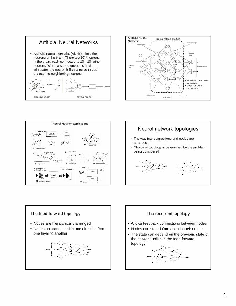
• Artificial neural networks (ANNs) mimic the neurons of the brain. There are 1011 neurons in the brain, each connected to 103- 105 other neurons. When a strong enough signal stimulates the neuron it fires a pulse through the axon to neighboring neurons
w1
wI-1
w2
wl
.
.
.
x1
x2
xl-1
xl
Σ Output
biological neuron artificial neuron
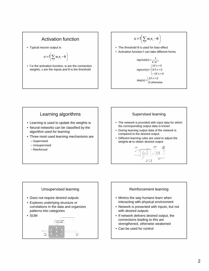
Artificial Neural NetworksInternal network structure
Hidden layer 1
Hidden layer 2Hidden layer 3
Network outputNetwork input
Neuron / NodeConnection weight
Input layer
Outputlayer
• Parallel and distributed computation
• Large number of connections
Artificial NeuralNetwork:
Σ
Σ
Σ
Σ
Σ
Σ
Σ
Σ
Σ
Σ
Σ
Σ
Σ
Σ
Σ
Σ
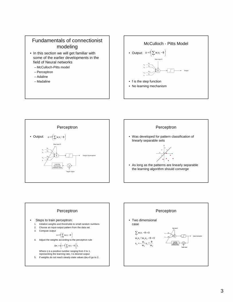
Neural Network applications
classification
clustering
regression prediction optimization
image analysis control
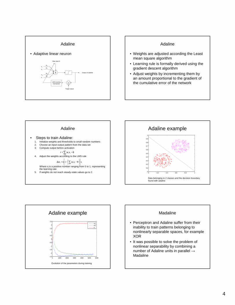
Neural network topologies
• The way interconnections and nodes are arranged
• Choice of topology is determined by the problem being considered
The feed-forward topology
• Nodes are hierarchically arranged• Nodes are connected in one direction from
one layer to another
The recurrent topology
• Allows feedback connections between nodes• Nodes can store information in their output
• The state can depend on the previous state of the network unlike in the feed-forward topology
2
Activation function
• Typical neuron output is
• f is the activation function, w are the connection weights, x are the inputs and θ is the threshold
−= ∑i
ii θxwfo
• The threshold θ is used for bias-effect• Activation function f can take different forms
>
=
<−=>
=
+= −
otherwise0
0xif1step(x)
0xif1
0xif0
0xif1
signum(x)
e11
sigmoid(x) x
−= ∑i
ii θxwfo
Learning algorithms
• Learning is used to update the weights w• Neural networks can be classified by the
algorithm used for learning• Three most used learning mechanisms are
– Supervised– Unsupervised– Reinforced
Supervised learning
• The network is provided with input data for which the corresponding output data is known
• During learning output data of the network is compared to the desired output
• Different learning rules are used to adjust the weights w to obtain desired output
Unsupervised learning
• Does not require desired outputs• Explores underlying structure or
correlations in the data and organizes patterns into categories
• SOM
Reinforcement learning
• Mimics the way humans learn when interacting with physical environment
• Network is presented with inputs, but not with desired outputs
• If network delivers desired output, the connections leading to this are strengthened, otherwise weakened
• Can be used for control
3
Fundamentals of connectionist modeling
• In this section we will get familiar with some of the earlier developments in the field of Neural networks – McCulloch-Pitts model– Perceptron– Adaline– Madaline
McCulloch - Pitts Model
• Output:
• f is the step function• No learning mechanism
w1
wI-1
w2
wl
.
.
.
x1
x2
xl-1
xl
Σ Output
Bias input θ
−= ∑i
ii θxwfo
Perceptron
• Output:
w1
wI-1
w2
wl
.
.
.
x1
x2
xl-1
xl
Σ Output of perceptron
Bias input θ
+-
Target output
LearningMechanism
(Hebbian Rule)
−= ∑i
ii θxwfo
Perceptron
• Was developed for pattern classification of linearly separable sets
• As long as the patterns are linearly separable the learning algorithm should converge
Perceptron
• Steps to train perceptron:1. Initialize weights and thresholds to small random numbers
2. Choose an input-output pattern from the data set
3. Compute output
4. Adjust the weights according to the perceptron rule
Where η is a positive number ranging from 0 to 1, representing the learning rate, t is desired output
5. If weights do not reach steady-state values ∆wi=0 go to 2.
−= ∑=
l
1iii θxwfo
ii
iii xθxwftη∆w
−−= ∑
Perceptron
• Two dimensional case
w2
w1x1
x2
Σ Output of perceptron
Bias input θ
+-
Target output
LearningMechanism
(Hebbian Rule)
w2
w1x1
x2
Σ Output of perceptron
Bias input θ
+-
Target output
LearningMechanism
(Hebbian Rule)
21
2
12
2211
iii
wθ
xww
x
0θxwxw
0θxw
+−=
=−+
=−∑
4
Adaline
• Adaptive linear neuron
w1
wI-1
w2
W l
.
.
.
x1
x2
xl-1
xl
Σ Output of adaline
Bias input θ
+-
Target output
LMS learningmechanism
Adaline
• Weights are adjusted according the Least mean square algorithm
• Learning rule is formally derived using the gradient descent algorithm
• Adjust weights by incrementing them by an amount proportional to the gradient of the cumulative error of the network
Adaline
• Steps to train Adaline:1. Initialize weights and thresholds to small random numbers2. Choose an input-output pattern from the data set3. Compute output before activation
4. Adjust the weights according to the LMS rule
Where η is a positive number ranging from 0 to 1, representingthe learning rate
5. If weights do not reach steady-state values go to 2.
∑=
−=l
1iii θxwr
ii
iii xθxwtη∆w
−−= ∑
Adaline example
0 0.2 0.4 0.6 0.8 10
0.1
0.2
0.3
0.4
0.5
0.6
0.7
0.8
0.9
1
Data belonging to 2 classes and the decision boundary found with adaline
Adaline example
Evolution of the parameters during training
0 1000 2000 3000 4000 5000 6000-2.5
-2
-1.5
-1
-0.5
0
0.5
1
1.5
2
2.5
w1w2θ
Madaline
• Perceptron and Adaline suffer from their inability to train patterns belonging to nonlinearly separable spaces, for example XOR
• It was possible to solve the problem of nonlinear separability by combining a number of Adaline units in parallel →Madaline
5
Madaline
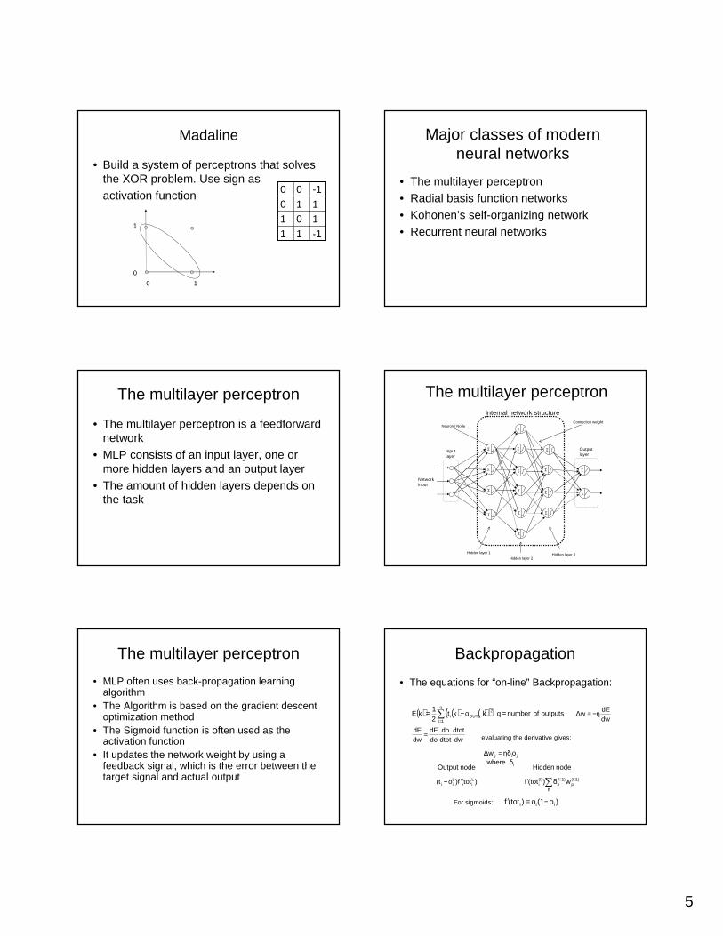
• Build a system of perceptrons that solves the XOR problem. Use sign asactivation function
-111
101110
-100
0 1
1
0
Major classes of modern neural networks
• The multilayer perceptron• Radial basis function networks• Kohonen’s self-organizing network• Recurrent neural networks
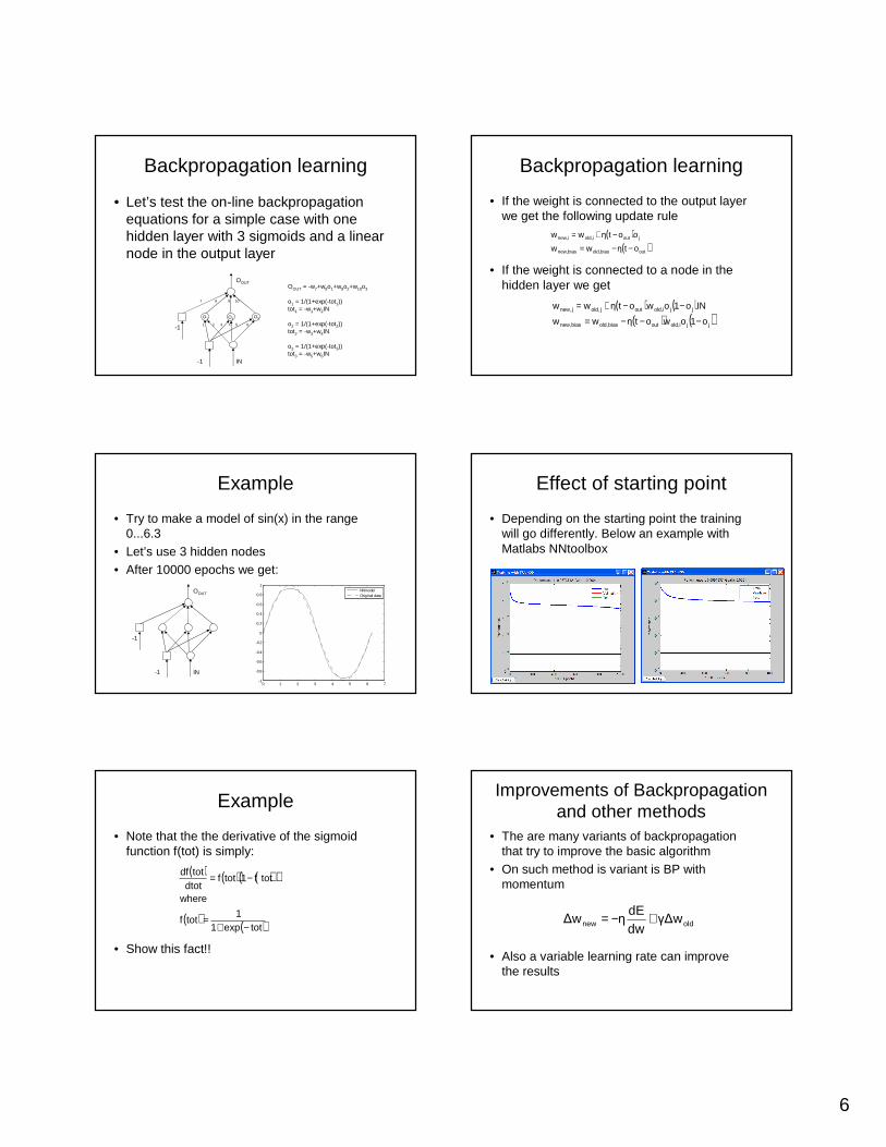
The multilayer perceptron
• The multilayer perceptron is a feedforwardnetwork
• MLP consists of an input layer, one or more hidden layers and an output layer
• The amount of hidden layers depends on the task
The multilayer perceptronInternal network structure
Hidden layer 1
Hidden layer 2Hidden layer 3
Network input
Neuron / NodeConnection weight
Input layer
Outputlayer
Σ
Σ
Σ
Σ
Σ
Σ
Σ
Σ
Σ
Σ
Σ
Σ
Σ
Σ
Σ
Σ
The multilayer perceptron
• MLP often uses back-propagation learning algorithm
• The Algorithm is based on the gradient descent optimization method
• The Sigmoid function is often used as the activation function
• It updates the network weight by using a feedback signal, which is the error between the target signal and actual output
Backpropagation
• The equations for “on-line” Backpropagation:
∑ ++′′−
=
p
1)(lp
1)(lp
(l)i
Li
Lii
i
jiij
wδ)(totf)(totf)o(t
node Hiddenδwhere
node Output
oηδ∆w
)o(1o)(totf iii −=′For sigmoids:
dwdE
η∆w −=( ) ( ) ( )( ) outputs of number q kokt21
kEq
1i
2iOUT,i =−= ∑
=
evaluating the derivative gives:dwdtot
dtotdo
dodE
dwdE =
6
Backpropagation learning
• Let’s test the on-line backpropagationequations for a simple case with one hidden layer with 3 sigmoids and a linear node in the output layer
-1 IN
-1 1 2 3 4 5 6
7 8 9 10
OOUT
O3O2O1
OOUT = -w7+w8o1+w9o2+w10o3
o1 = 1/(1+exp(-tot1))tot1 = -w1+w2IN
o2 = 1/(1+exp(-tot2))tot2 = -w3+w4IN
o3 = 1/(1+exp(-tot3))tot3 = -w5+w6IN
Backpropagation learning
• If the weight is connected to the output layer we get the following update rule
• If the weight is connected to a node in the hidden layer we get
( )( )outbiasold,biasnew,
joutiold,inew,
otηww
ootηww
−−=
−+=
( ) ( )( ) ( )jjiold,outbiasold,biasnew,
jjiold,outjold,jnew,
o1owotηww
INo1owotηww
−−−=
−−+=
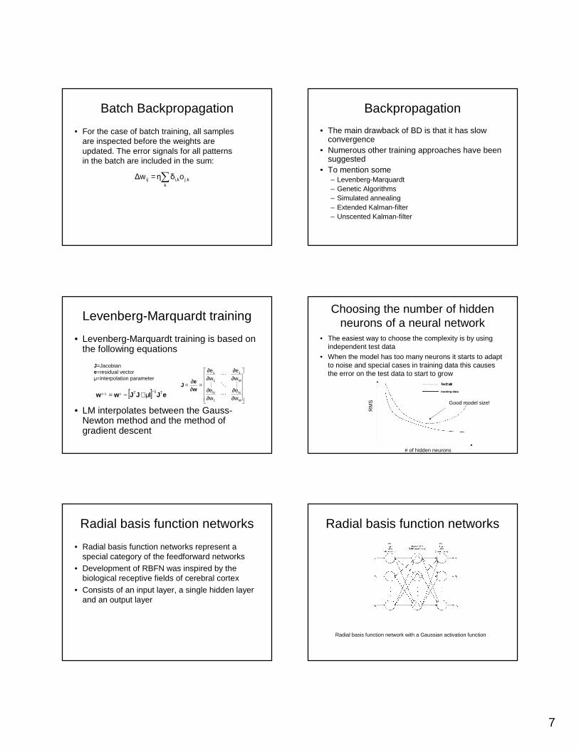
Example
• Try to make a model of sin(x) in the range 0...6.3
• Let’s use 3 hidden nodes• After 10000 epochs we get:
-1 IN
-1
OOUT
0 1 2 3 4 5 6 7-1
-0.8
-0.6
-0.4
-0.2
0
0.2
0.4
0.6
0.8
1
NNmodelOriginal data
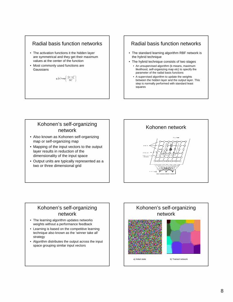
Effect of starting point
• Depending on the starting point the training will go differently. Below an example with Matlabs NNtoolbox
Example
• Note that the the derivative of the sigmoid function f(tot) is simply:
• Show this fact!!
( ) ( ) ( )( )
( ) ( )totexp11
totf
where
totf1totfdtot
totdf
−+=
−=
Improvements of Backpropagationand other methods
• The are many variants of backpropagationthat try to improve the basic algorithm
• On such method is variant is BP with momentum
• Also a variable learning rate can improve the results
oldnew γ∆wdwdE
η∆w +−=
7
Batch Backpropagation
• For the case of batch training, all samples are inspected before the weights are updated. The error signals for all patterns in the batch are included in the sum:
∑=k
j.kki,ij oδη∆w
Backpropagation
• The main drawback of BD is that it has slowconvergence
• Numerous other training approaches have been suggested
• To mention some – Levenberg-Marquardt– Genetic Algorithms– Simulated annealing– Extended Kalman-filter– Unscented Kalman-filter
Levenberg-Marquardt training
• Levenberg-Marquardt training is based on the following equations
• LM interpolates between the Gauss-Newton method and the method of gradient descent
[ ] eJIJJww T1T µk1k−
+−=+
∂∂
∂∂
∂∂
∂∂
=∂∂=
M
N
1
N
M
1
1
1
we
we
we
we
⋯
⋮⋱⋮
⋯
we
J
J=Jacobiane=residual vectorµ=interpolation parameter
Choosing the number of hidden neurons of a neural network
• The easiest way to choose the complexity is by using independent test data
• When the model has too many neurons it starts to adapt to noise and special cases in training data this causes the error on the test data to start to grow
# of hidden neurons
RM
S
training data
Good model size!
Radial basis function networks
• Radial basis function networks represent a special category of the feedforward networks
• Development of RBFN was inspired by the biological receptive fields of cerebral cortex
• Consists of an input layer, a single hidden layer and an output layer
Radial basis function networks
Radial basis function network with a Gaussian activation function
8
Radial basis function networks
• The activation functions it the hidden layer are symmetrical and they get their maximum values at the center of the function
• Most commonly used functions are Gaussians
( )
−−= 2
i
2
ii 2σ
vxexpxg
Radial basis function networks
• The standard learning algorithm RBF network is the hybrid technique
• The hybrid technique consists of two stages• An unsupervised algorithm (k-means, maximum
likelihood, self-organizing map etc) to specify the parameter of the radial basis functions
• A supervised algorithm to update the weights between the hidden layer and the output layer. This step is normally performed with standard least squares
Kohonen’s self-organizing network
• Also known as Kohonen self-organizing map or self-organizing map
• Mapping of the input vectors to the output layer results in reduction of the dimensionality of the input space
• Output units are typically represented as a two or three dimensional grid
Kohonen network
Kohonen’s self-organizing network
• The learning algorithm updates networks weights without a performance feedback
• Learning is based on the competitive learning technique also known as the ’winner take all’strategy
• Algorithm distributes the output across the input space grouping similar input vectors
Kohonen’s self-organizing network
a) Initial state b) Trained network
9
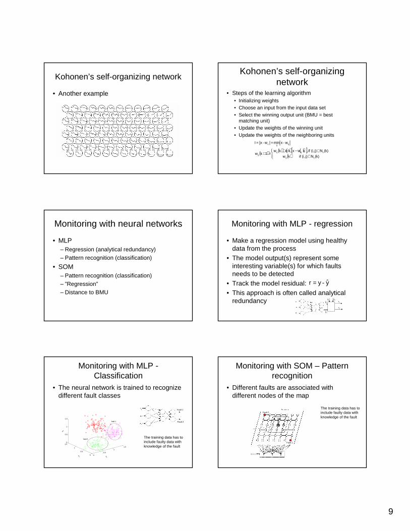
Kohonen’s self-organizing network
• Another example
Kohonen’s self-organizing network
• Steps of the learning algorithm• Initializing weights• Choose an input from the input data set• Select the winning output unit (BMU = best
matching unit)• Update the weights of the winning unit• Update the weights of the neighboring units
( ) ( ) ( ) ( )[ ]( )
∉∈−+
=+
==
(k)N j)(i, if kw
(k)N j)(i, if ,kwxkαkw1kw
w-xminw-x I
cij
cijijij
ijijc
Monitoring with neural networks
• MLP– Regression (analytical redundancy)– Pattern recognition (classification)
• SOM– Pattern recognition (classification)– ”Regression”– Distance to BMU
Monitoring with MLP - regression
• Make a regression model using healthy data from the process
• The model output(s) represent some interesting variable(s) for which faults needs to be detected
• Track the model residual:• This approach is often called analytical
redundancy
y -yr ˆ=
1y
2y
y1 y2r1
r2
Monitoring with MLP -Classification
• The neural network is trained to recognize different fault classes
Fault 1
Fault 2
0
0.5
1
1.5
0
0.5
1
1.50
0.5
1
1.5
x1
x2
x 3
fault 1
fault 2The training data has to include faulty data with knowledge of the fault
Monitoring with SOM – Pattern recognition
• Different faults are associated with different nodes of the map
The training data has to include faulty data with knowledge of the fault
Fault 1
Fault 2
10
Monitoring with SOM – ”regression”
• The model is based on fault free data• When new data is fed to the model the
BMU is found based on a subset of the input vector (the monitored variable y is left out)
• Check the value of y for the BMU• Calculate the residual between measured
y and y from BMU
Monitoring with SOM – Distance to BMU
• Find the BMU for the given input • Calculate distance between BMU and
input• If the distance exceeds the threshold a
fault has been detected
Recurrent neural networks
• With standard feed-forward networks only static mappings can be made.
• The models are without memory - they don’t have a state.
• In some cases this is not enough. E.g. if long term prediction capabilities and effective noise handling are important
• By introducing feedback to our networks we enable true dynamic modeling
Recurrent neural networks
• In recurrent neural networks, some outputs are directed back as inputs to nodes in the same or preceding layer
• These models have a memory – a state
• They are much more challenging to train
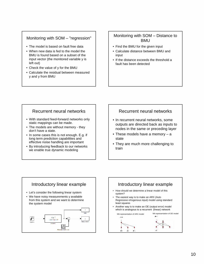
Introductory linear example
• Let’s consider the following linear system• We have noisy measurements y available
from this system and we want to determine the system model
input u
Introductory linear example• How should we determine a linear model of this
system?• The easiest way is to make an ARX (Auto
Regressive eXogenous input) model using standard least squares
• Another way is to make an OE (output error) model which is analogous to a recurrent (linear) network
NN representation of OE modelNN representation of ARX model
11
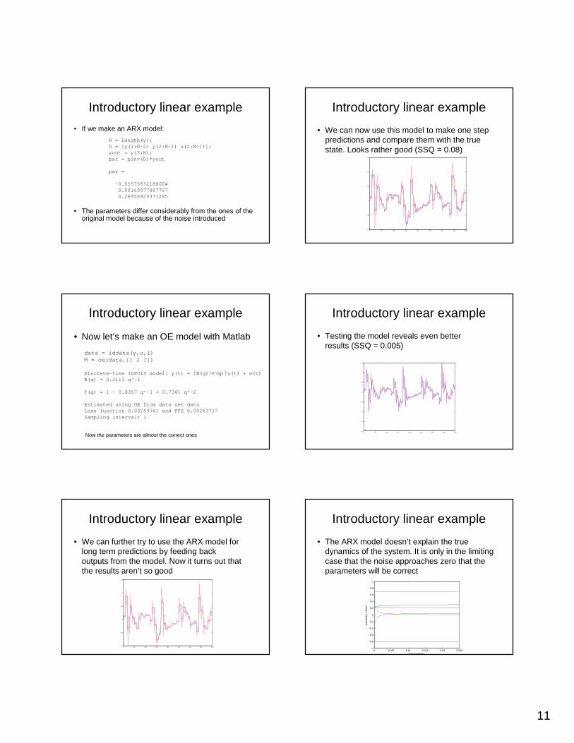
Introductory linear example
• If we make an ARX model:
• The parameters differ considerably from the ones of the original model because of the noise introduced
N = length(y);D = [y(1:N-2) y(2:N-1) u(2:N-1)];yout = y(3:N);par = pinv(D)*yout
par =
-0.055758321880040.001690778877670.26950929371295
Introductory linear example
• We can now use this model to make one step predictions and compare them with the true state. Looks rather good (SSQ = 0.08)
0 50 100 150 200 250 300 350 400-0.1
-0.05
0
0.05
0.1
0.15
Introductory linear example
• Now let’s make an OE model with Matlab
data = iddata(y,u,1)M = oe(data,[1 2 1])
Discrete-time IDPOLY model: y(t) = [B(q)/F(q)]u(t) + e(t)B(q) = 0.2113 q^-1
F(q) = 1 - 0.8357 q^-1 + 0.7361 q^-2
Estimated using OE from data set data Loss function 0.00259761 and FPE 0.00263717 Sampling interval: 1
Now the parameters are almost the correct ones
Introductory linear example
• Testing the model reveals even better results (SSQ = 0.005)
0 50 100 150 200 250 300 350 400-0.2
-0.15
-0.1
-0.05
0
0.05
0.1
0.15
Introductory linear example
• We can further try to use the ARX model for long term predictions by feeding back outputs from the model. Now it turns out that the results aren’t so good
0 50 100 150 200 250 300 350 400-0.1
-0.05
0
0.05
0.1
0.15
Introductory linear example
• The ARX model doesn’t explain the true dynamics of the system. It is only in the limiting case that the noise approaches zero that the parameters will be correct
0 0.005 0.01 0.015 0.02 0.025-1
-0.8
-0.6
-0.4
-0.2
0
0.2
0.4
0.6
0.8
1
noise variance
para
met
er v
alue
s
12
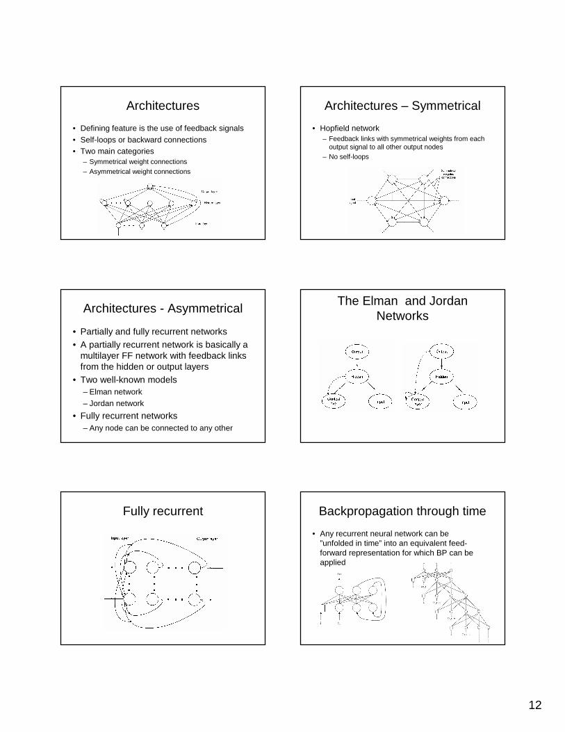
Architectures
• Defining feature is the use of feedback signals• Self-loops or backward connections• Two main categories
– Symmetrical weight connections– Asymmetrical weight connections
Architectures – Symmetrical
• Hopfield network– Feedback links with symmetrical weights from each
output signal to all other output nodes– No self-loops
Architectures - Asymmetrical
• Partially and fully recurrent networks• A partially recurrent network is basically a
multilayer FF network with feedback links from the hidden or output layers
• Two well-known models– Elman network– Jordan network
• Fully recurrent networks– Any node can be connected to any other
The Elman and Jordan Networks
Fully recurrent Backpropagation through time
• Any recurrent neural network can be ”unfolded in time” into an equivalent feed-forward representation for which BP can be applied
13
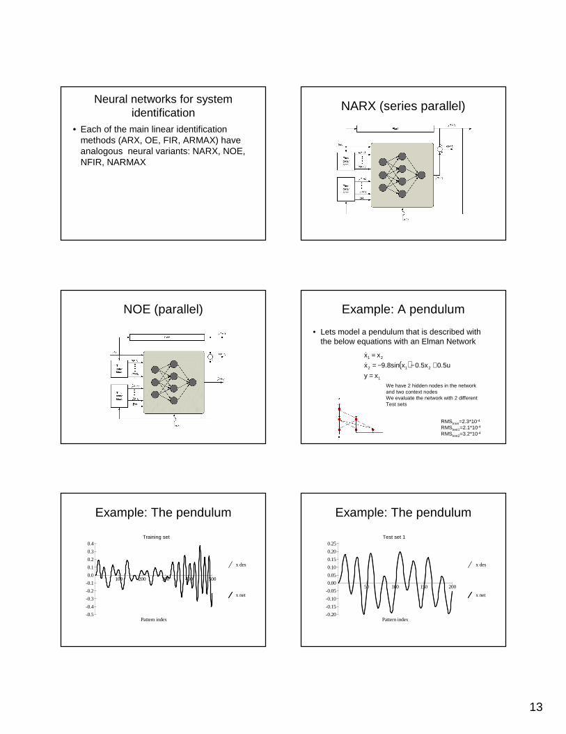
Neural networks for system identification
• Each of the main linear identification methods (ARX, OE, FIR, ARMAX) have analogous neural variants: NARX, NOE, NFIR, NARMAX
NARX (series parallel)
NOE (parallel) Example: A pendulum
• Lets model a pendulum that is described with the below equations with an Elman Network
( )1
212
21
xy
0.5u0.5xx9.8sinx
xx
=+−−=
=ɺ
ɺ
RMStrain=2.3*10-4
RMStest1=2.1*10-4
RMStest2=3.2*10-4
We have 2 hidden nodes in the networkand two context nodesWe evaluate the network with 2 different Test sets
Example: The pendulum
x des
x net
Pattern index
0.0
0.1
0.2
0.3
0.4
-0.1
-0.2
-0.3
-0.4
-0.5
100 200 300 400 500
Training set
Example: The pendulum
x des
x net
Pattern index
0.00
0.05
0.10
0.15
0.20
0.25
-0.05
-0.10
-0.15
-0.20
50 100 150 200
Test set 1
14
Example: The pendulum
x des
x net
Pattern index
0.00
0.05
0.10
0.15
0.20
0.25
-0.05
-0.10
-0.15
-0.20
50 100 150 200
Test set 2
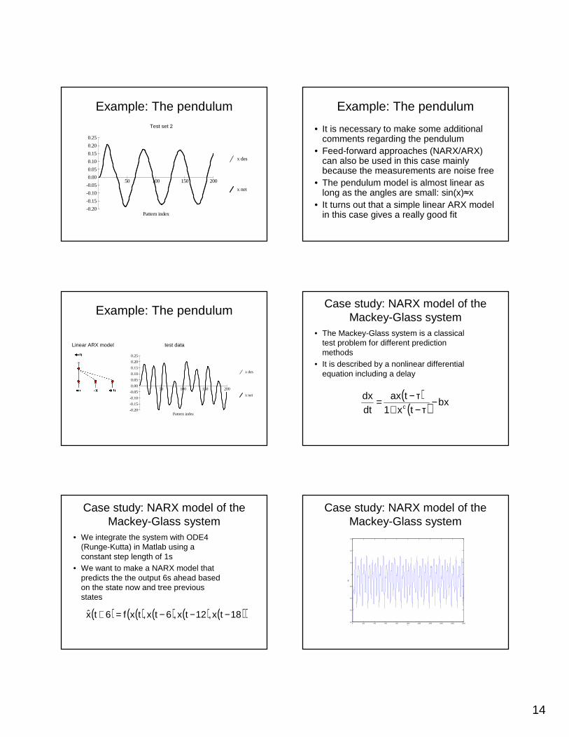
Example: The pendulum
• It is necessary to make some additional comments regarding the pendulum
• Feed-forward approaches (NARX/ARX) can also be used in this case mainly because the measurements are noise free
• The pendulum model is almost linear as long as the angles are small: sin(x)≈x
• It turns out that a simple linear ARX model in this case gives a really good fit
Example: The pendulum
x des
x net
Pattern index
0.00
0.05
0.10
0.15
0.20
0.25
-0.05
-0.10
-0.15
-0.20
50 100 150 200
test dataLinear ARX model
Case study: NARX model of the Mackey-Glass system
• The Mackey-Glass system is a classical test problem for different prediction methods
• It is described by a nonlinear differential equation including a delay
( )( ) bxτtx1τtax
dtdx
c −−+
−=
Case study: NARX model of the Mackey-Glass system
• We integrate the system with ODE4 (Runge-Kutta) in Matlab using a constant step length of 1s
• We want to make a NARX model that predicts the the output 6s ahead based on the state now and tree previous states
( ) ( ) ( ) ( ) ( )( )18tx,12tx,6tx,txf6tx −−−=+ˆ
Case study: NARX model of the Mackey-Glass system
0 200 400 600 800 1000 1200 1400 1600 1800 20000.2
0.4
0.6
0.8
1
1.2
1.4
1.6
t
x(t)
15
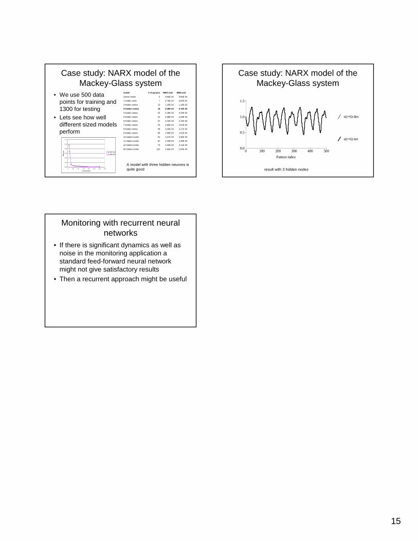
Case study: NARX model of the Mackey-Glass system
• We use 500 data points for training and 1300 for testing
• Lets see how well different sized models perform
0.00
0.02
0.04
0.06
0.08
0.10
0.12
0 20 40 60 80 100 120 140
# of parameters
RM
S e
rror
RMS train
RMS test
1.94E-031.52E-0312120 hidden nodes
2.11E-032.03E-037312 hidden nodes
2.30E-032.15E-036711 hidden nodes
2.49E-032.47E-036110 hidden nodes
2.81E-032.55E-03559 hidden nodes
3.17E-033.19E-03498 hidden nodes
3.91E-033.85E-03437 hidden nodes
4.14E-034.16E-03376 hidden nodes
4.44E-034.46E-03315 hidden nodes
5.33E-035.28E-03254 hidden nodes
6.15E-036.28E-03193 hidden nodes
1.14E-021.16E-02132 hidden nodes
6.82E-026.76E-0271 hidden node
9.66E-029.62E-025Linear model
RMS testRMS train# of paramsmodel
A model with three hidden neurons isquite good
Case study: NARX model of the Mackey-Glass system
x(t+6) des
x(t+6) net
Pattern index
0.0
0.5
1.0
1.5
0 100 200 300 400 500
result with 3 hidden nodes
Monitoring with recurrent neural networks
• If there is significant dynamics as well as noise in the monitoring application a standard feed-forward neural network might not give satisfactory results
• Then a recurrent approach might be useful