IEEE TRANSACTIONS ON PATTERN ANALYSIS AND MACHINE INTELLIGENCE, VOL. 20, NO. 2, FEBRUARY 1998 139

Closed-Loop Object Recognition UsingReinforcement Learning

Jing Peng and Bir Bhanu, Fellow, IEEE

Abstract—Current computer vision systems whose basic methodology is open-loop or filter type typically use image segmentationfollowed by object recognition algorithms. These systems are not robust for most real-world applications. In contrast, the systempresented here achieves robust performance by using reinforcement learning to induce a mapping from input images tocorresponding segmentation parameters. This is accomplished by using the confidence level of model matching as a reinforcementsignal for a team of learning automata to search for segmentation parameters during training. The use of the recognition algorithmas part of the evaluation function for image segmentation gives rise to significant improvement of the system performance byautomatic generation of recognition strategies. The system is verified through experiments on sequences of indoor and outdoorcolor images with varying external conditions.

Index Terms—Adaptive color image segmentation, function optimization, generalized learning automata, learning in computervision, model-based object recognition, multiscenario recognition, parameter learning, recognition feedback, segmentationevaluation.

—————————— ✦ ——————————

1 INTRODUCTION

MAGE segmentation, feature extraction, and modelmatching are the key building blocks of a computer

vision system for model-based object recognition [8], [23].The tasks performed by these building blocks are charac-terized as the low (segmentation), intermediate (featureextraction), and high (model matching) levels of com-puter vision. The goal of image segmentation is to extractmeaningful objects from an image. It is essentially apixel-based processing. Model matching uses a represen-tation such as shape features obtained at the intermediatelevel for recognition. It requires explicit shape models ofthe object to be recognized. There is an abstraction of im-age information as we move from low to high levels andthe processing becomes more knowledge-based or goal-directed.

Although there is an abundance of proposed computervision algorithms for object recognition, there have beenfew systems that achieve good performance for practicalapplications, for most such systems do not adapt to chang-ing environments [2]. The main difficulties, typically asso-ciated with systems that are mostly open-loop or filter type,can be characterized as follows.

1) The fixed set of parameters used in various vision al-gorithms often leads to ungraceful degradation inperformance.

2) The image segmentation, feature extraction, and se-lection are generally carried out as preprocessingsteps to object recognition algorithms for modelmatching. These steps totally ignore the effects of the

earlier results (image segmentation and feature ex-traction) on the future performance of the recognitionalgorithm.

3) Generally, the criteria used for segmentation andfeature extraction require elaborate human designs.When the conditions for which they are designed arechanged slightly, these algorithms fail. Furthermore,the criteria themselves can be a subject of debate [3].

4) Object recognition is a process of making sequences ofdecisions, i.e., applying various image analysis algo-rithms. Often the usefulness of a decision or the re-sults of an individual algorithm can only be deter-mined by the final outcome (e.g., matching confi-dence) of the recognition process. This is also knownas “vision-complete” problem [7], i.e., one cannotreally assign labels to the image without the knowl-edge of which parts of the image correspond to whatobjects.

This paper presents a learning-based vision frameworkin which the above problems can be adequately ad-dressed. The underlying theory is that any recognitionsystem whose decision criteria for image segmentationand feature extraction, etc., are developed autonomouslyfrom the outcome of the final recognition might transcendall these problems. A direct result of the theory is that thelow- and high-level components of a vision system mustinteract to achieve robust performance under changingenvironmental conditions. Our system accomplishes thisby incorporating a reinforcement learning mechanism tocontrol the interactions of different levels within it. Spe-cifically, the system takes the output of the recognitionalgorithm and uses it as a feedback to influence the per-formance of the segmentation process. As a result, therecognition performance can be significantly improvedover time with this method.

0162-8828/98/$10.00 © 1998 IEEE

¥¥¥¥¥¥¥¥¥¥¥¥¥¥¥¥

• The authors are with the College of Engineering, University of California,Riverside, CA 92521. E-mail: {jp, bhanu}@vislab.ucr.edu.

Manuscript received 11 Apr. 1996; revised 1 Dec. 1997. Recommended for accep-tance by L. Shapiro.For information on obtaining reprints of this article, please send e-mail to:tpami@computer.org, and reference IEEECS Log Number 106038.

I

140 IEEE TRANSACTIONS ON PATTERN ANALYSIS AND MACHINE INTELLIGENCE, VOL. 20, NO. 2, FEBRUARY 1998

One attractive feature of the approach is that it includesthe matching or recognition component as part of theevaluation function for image segmentation in a systematicway. An additional strength is that the system develops itsindependent decision criteria (segmentation parameters) tobest serve the underlying recognition task. It should be em-phasized that our interest is not in a simple mixture oflearning and computer vision, but rather in the principledintegration of the two fields at the algorithmic level. Notethat the goal here is to seek a general mapping from imagesto parameter settings of various algorithms based on recog-nition results. To our knowledge, however, no such approachexists in the computer vision field. Also, there is no work inthe neural network field (e.g., application of Neocognition[10]) for parameter adaptation of segmentation algorithms [3].

This work is most closely related to the work by Bhanu et al.[3], [5], [6], where they describe a system that uses geneticand hybrid algorithms for learning segmentation parameters.However, the recognition algorithm is not part of the evalua-tion function for segmentation in their system. The genetic orhybrid algorithms simply search for a set of parameters thatoptimizes a prespecified evaluation function (based on globaland local segmentation evaluation) that may not best servethe overall goal of robust object recognition. Furthermore, thepapers assume that the location of the object in the image isknown for specific photointerpretation application. In ourwork, we do not make such an assumption. We use explicitgeometric model of an object, represented by its polygonalapproximation, to recognize it in the image.

In addition, Wang and Binford [24] and Ramesh [21]have investigated statistical methods for performanceevaluation and tuning free parameters of an algorithm.Wang and Binford [24] presented a theoretical analysis foredge estimation and showed how one can select the gradi-ent threshold (tuning parameter) for edge detection.Ramesh [21] has developed a methodology for the analysisof computer vision algorithms and systems using systemengineering principles. To characterize the performance ofan algorithm he developed statistical models for ideal im-age features (such as edges and corners) and random per-turbations at input/output of an algorithm. Additionally,prior distributions for image features are also obtained.Using these models and a criterion function, he can char-acterize the performance of a given algorithm as a functionof tuning parameters and determine these parametersautomatically. Our approach presented in this paper differssignificantly from Ramesh’s [21] approach.

1) Ramesh’s approach is open loop, while our approach isclosed loop. In our approach, recognition results de-termine how the segmentation parameters should bechanged.

2) Ramesh is tuning the parameters of an individual al-gorithm—it is known that the optimization of indi-vidual components does not necessarily give the op-timal results for the system. We are working with acomplete recognition system (segmentation, featureextraction, and model matching components) andimproving the performance of the complete system.

3) Ramesh builds elaborate statistical models (usingthe training data) that require complex processes of

annotation and approximating the measured distribu-tions with mathematical functions to be used later. Ourlearning approach does not build explicit statisticalmodels. It uses geometrical models during modelmatching.

4) It is relatively easier to build statistical models for al-gorithms like edge and corner detection. For complexalgorithms like Phoenix, it is difficult to model the“perfect” algorithm behavior analytically, since the per-formance of segmentation depends nonlinearly withthe changes in parameter values, and there are someheuristics used in the algorithm. Considering the abovefactors, our approach is more general for the problemthat we are trying to solve. We have developed alearning-based approach presented in this paper.

Section 2 describes a general framework for reinforcementlearning-based adaptive image segmentation. Section 3 de-scribes the reinforcement learning paradigm and the par-ticular reinforcement learning algorithm employed in oursystem. Section 4 presents the experimental results evalu-ating the system, and Section 5 concludes the paper. Twoappendices describe the basic segmentation and modelmatching algorithms used to perform experiments forclosed-loop object recognition using reinforcement learning.

2 REINFORCEMENT LEARNING SYSTEM FORSEGMENTATION PARAMETER ESTIMATION

2.1 The ProblemConsider the problem of recognizing an object in an inputimage, assuming that the model of the object is given, andthat the precise location of the object in the image is un-known. The conventional method for the recognition prob-lem, shown in Fig. 1, is to first segment the input image,then extract and select appropriate features from the seg-mented image, and finally perform model matching usingthese features. If we assume that the matching algorithmproduces a real valued output indicating the degree of suc-cess upon its completion, then it is natural to use this realvalued output as feedback to influence the performance ofsegmentation and feature extraction, so as to bring aboutsystem’s earlier decisions favorable for more accuratemodel matching. The rest of the paper describes a rein-forcement learning-based vision system to achieve just that.

Fig. 1. Conventional multilevel system for object recognition.

PENG AND BHANU: CLOSED-LOOP OBJECT RECOGNITION USING REINFORCEMENT LEARNING 141

2.2 Learning to Segment ImagesOur current investigation into reinforcement learning-basedvision systems is focused on the problem of learning tosegment images. An important characteristic of our ap-proach is that the segmentation process takes into accountthe biases of the recognition algorithm to develop its owndecision strategies. A consequence of this is that the effec-tive search space of segmentation parameters can be dra-matically reduced. As a result, more accurate and efficientsegmentation and recognition performance can be expected.

2.2.1 Image SegmentationWe begin with image segmentation [13], because it is anextremely important and difficult low-level task. All subse-quent interpretation tasks including object detection, fea-ture extraction, object recognition, and classification relyheavily on the quality of the segmentation process. The dif-ficulty arises for image segmentation when only local imageproperties are used to define the region-of-interest for eachindividual object. It is known [2], [9] that correct localiza-tion may not always be possible. Thus, a good image seg-mentation cannot be done by grouping parts with similarimage properties in a purely bottom-up fashion. Difficultiesalso arise when segmentation performance needs to beadapted to the changes in image quality, which is affectedby variations in environmental conditions, imaging devices,lighting, etc. The following are the key characteristics [3] ofthe image segmentation problem:

1) When presented with a new image, selecting the ap-propriate set of algorithm parameters is the key to ef-fectively segmenting the image.

2) The parameters within most segmentation algorithmstypically interact in a complex, nonlinear fashion,which makes it difficult to model the parameters’ be-havior analytically.

3) The variations between images cause changes in thesegmentation results, the objective function that rep-resents segmentation quality varies from image toimage. Also, there may not be a consensus on seg-mentation quality measures.

2.2.2 Our ApproachEach combination of segmentation parameters produces,for a given input, a unique segmentation image fromwhich a confidence level of model matching can be com-puted. The simplest way to acquire high payoff parametercombinations is through trial and error. That is, generate acombination of parameters, compute the matching confi-dence, generate another combination of parameters, andso on, until the confidence level has exceeded a giventhreshold. Better yet, if a well-defined evaluation functionover the segmentation parameter space is available, thenlocal gradient methods, such as hill-climbers, suffice.While the trial-and-error methods suffer from excessivedemand for computational resources, such as time andspace, the gradient methods suffer from the unrealisticrequirement for an evaluation function. In contrast, rein-forcement learning performs trials and errors, yet does notdemand excessive computational resources; it performs hill-climbing in a statistical sense, yet does not require an

evaluation function. In addition, it can generalize overunseen images as we shall see later. Furthermore, it can beeasily adapted to multilevel computer vision systems. It isalso feasible to construct fast, parallel devices to imple-ment this technique for real-time applications. It thus fitsour goal nicely here.

Fig. 2 depicts the conceptual diagram of our reinforce-ment learning-based object recognition system that ad-dresses the parameter selection problem encountered inthe image segmentation task by using the recognition al-gorithm itself as part of the evaluation function for imagesegmentation. Note that the reinforcement learning com-ponent employs a particular reinforcement learning algo-rithm that will be described in the next section. Fig. 3shows the main steps of the algorithm we use, where thealgorithm terminates when either the number of itera-tions reaches a prespecified value (N) or the averagematching confidence over entire training data (denotedby rr) has exceeded a given threshold, called Rth . Notethat n denotes the number of images in the training set. Inthe event that the number of iterations has exceeded N,we will say that the object is not present in the image.Also, for simplicity, we assume that only one instance ofthe model is present in the image. Multiple instances ofthe model can be recognized by slight modification of thealgorithm.

Fig. 2. Reinforcement learning-based multilevel system for objectrecognition.

• LOOP:1. rr = 0 (rr: average matching confidence)2. For each image i in the training set do(a) Segment image i using current segmentation

parameters(b) Perform noise clean up(c) Get segmented regions (also called blobs or con-

nected components)(d) Perform feature extraction for each blob to obtain

token sets(e) Compute the matching of each token set against

stored model and return the highest confidencelevel, r

(f) rr = rr + r(g) Obtain new parameters for the segmentation algo-

rithm using r as reinforcement for the reinforcementlearning algorithm

• UNTIL number of iterations is equal to N or rr n Rth≥

Fig. 3. Main steps of the reinforcement learning-based object recogni-tion algorithm.

142 IEEE TRANSACTIONS ON PATTERN ANALYSIS AND MACHINE INTELLIGENCE, VOL. 20, NO. 2, FEBRUARY 1998

3 REINFORCEMENT LEARNING

In this section, we begin with a brief overview of the rein-forcement learning technique. We then describe reinforce-ment learning algorithms applicable to our task and themodifications of these algorithms to effectively solve theproblem identified in Section 2.1.

Reinforcement learning is an important machine learn-ing paradigm. It is a framework for learning to make se-quences of decisions in an environment [1]. It is distinctfrom supervised learning, like the popular backpropagationalgorithm, in that feedback it receives is evaluative insteadof instructive. That is, for supervised learning, the system ispresented with the correct output for each input instance,while for reinforcement learning, the system produces aresponse that is then evaluated using a scalar indicating theappropriateness of the response. As an example, a chessplaying computer program that uses the outcome of a gameto improve its performance is a reinforcement learningsystem. Knowledge about an outcome is useful for evalu-ating the total system’s performance, but it says nothingabout which actions were instrumental for the ultimate winor loss. In general, reinforcement learning is more widelyapplicable than supervised learning, since any supervisedlearning problem can be treated as a reinforcement learningproblem.

In the reinforcement learning framework, a learningsystem is given, at each time step, inputs describing its en-vironment. The system then makes a decision based onthese inputs, thereby causing the environment to deliver tothe system a reinforcement. The value of this reinforcementdepends on the environmental state, the system’s decision,and possibly random disturbances. In general, reinforce-ment measuring the consequences of a decision can emergeat a multitude of times after a decision is made. A distinc-tion can be made between associative and nonassociativereinforcement learning. In the nonassociative paradigm,reinforcement is the only information the system receivesfrom its environment. Whereas, in the associative para-digm, the system receives input information that indicatesthe state of its environment as well as reinforcement. Insuch learning systems, a “state” is a unique representationof all previous inputs to a system. In computer vision, this

state information corresponds to current input image. Ourobject recognition applications require us to take into ac-count the changes appearing in the input images. The ob-jective of the system is to select sequences of decisions tomaximize the sum of future reinforcement (possibly dis-counted) over time. It is interesting to note that, for a givenstate, an associative reinforcement learning problem be-comes a nonassociative learning problem.

As noted above, a complication to reinforcement learn-ing is the timing of reinforcement. In simple tasks, the sys-tem receives, after each decision, reinforcement indicatingthe goodness of that decision. Immediate reinforcementoccurs commonly in function optimization problems. Inmore complex tasks, however, reinforcement is often tem-porally delayed, occurring only after the execution of a se-quence of decisions. Delayed reinforcement learning is im-portant because, in many problem domains, immediatereinforcement regarding the value of a decision may notalways be available. For example, in object recognition, thegoodness of segmentation is not known until the recogni-tion decision has been made. Delayed reinforcement learn-ing is attractive and can play an important role in computervision [20]. Because delayed reinforcement learning doesnot concern us here, we do not discuss this subject further.

In this paper, we instead concentrate on the immediatereinforcement learning paradigm, for it provides a simple,yet principled framework within which the main problemsidentified above can be properly addressed. It also serves asa stepping stone for better understanding of the issues in-volved in computer vision that need to be addressed bydelayed reinforcement learning [20]. A well-understoodmethod in immediate reinforcement learning is the REIN-FORCE algorithm [25], a class of connectionist reinforce-ment learning algorithms, that performs stochastic hill-climbing, and which is the subject of our paper.

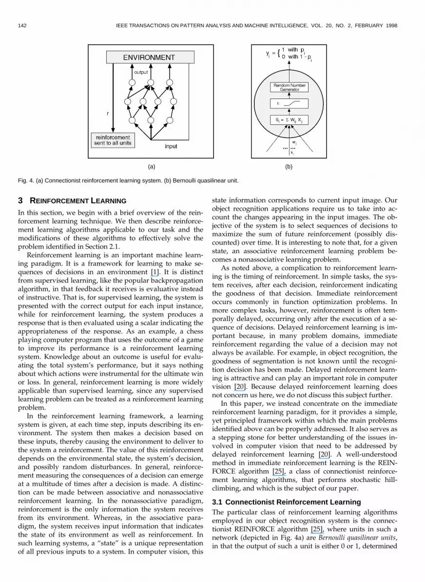
3.1 Connectionist Reinforcement LearningThe particular class of reinforcement learning algorithmsemployed in our object recognition system is the connec-tionist REINFORCE algorithm [25], where units in such anetwork (depicted in Fig. 4a) are Bernoulli quasilinear units,in that the output of such a unit is either 0 or 1, determined

(a) (b)

Fig. 4. (a) Connectionist reinforcement learning system. (b) Bernoulli quasilinear unit.

PENG AND BHANU: CLOSED-LOOP OBJECT RECOGNITION USING REINFORCEMENT LEARNING 143

stochastically using the Bernoulli distribution with parameterp = f(s), where f is the logistic function,

f(s) = 1/(1 + exp(-s)) (1)

and s w xi ii= Â is the usual weighted summation of input

values to that unit. For such a unit, p represents its prob-ability of choosing one as its output value. Fig. 4b depictsthe ith unit.

In the general reinforcement learning paradigm, thenetwork generates an output pattern and the environmentresponds by providing the reinforcement r as its evalua-tion of that output pattern, which is then used to drivethe weight changes according to the particular reinforce-ment learning algorithm being used by the network. Forthe Bernoulli quasilinear units used in this research, theREINFORCE algorithm prescribes weight incrementsequal to

Dw r b y p xij i i j= - -a1 62 7 (2)

where a is a positive learning rate, b serves as a reinforce-ment baseline, x j is the input to each Bernoulli unit, yi is the

output of the ith Bernoulli unit, and pi is an internal pa-

rameter to a Bernoulli random number generator (see (1)).Note that i takes values from one to n and j from one to m,where n and m are the number of the units in the networkand the number of input features, respectively.

It can be shown [25] that, regardless of how b is com-puted, whenever it does not depend on the immediatelyreceived reinforcement value r, and when r is sent to all theunits in the network, such an algorithm satisfies

E E rDW W WW= B = B= —a (3)

where E denotes the expectation operator, W represents theweight matrix (n ¥ (m + 1), m + 1 because of m inputs plus abias) of the network, and DW is the change of the weightmatrix. A reinforcement learning algorithm satisfying (3)has the property that the algorithm statistically climbs thegradient of expected reinforcement in weight space. That is,the algorithm is guaranteed to converge to a local optimum.

For adapting parameters of the segmentation algorithm, itmeans that the segmentation parameters change in the di-rection along which the expected matching confidence in-creases. The next two subsections describe the particularnetwork and the algorithm used in this paper.

3.2 The Team ArchitectureWe use a form of trial generating network in which all of theunits are output units and there are no interconnections be-tween them. This degenerate class of network corresponds towhat is called a team of automata in the literature on stochas-tic learning automata [18]. We, therefore, call these networksas teams of Bernoulli quasilinear units. The main thrust of thearchitecture is its simplicity and its generality as a functionapproximator. Fig. 5 depicts the team network used here,which corresponds directly to the reinforcement learningcomponent in Fig. 2. Each segmentation parameter is repre-sented by a set of Bernoulli quasilinear units, and the outputof each unit is binary as we have described earlier.

For any Bernoulli quasilinear unit, the probability that itproduces a 1 on any particular trial given the value of theweight matrix W is

Pr y p f se

i i i si= = = =

+-

11

1W< A 2 7

where s w xi ij jj= Â . Because all units pick their outputs

independently, it follows that, for such a team of Bernoulliquasilinear units, the probability of any particular outputvector y(t), corresponding to an instance of segmentationparameters, conditioned on the current value of the weightmatrix W is given by

Pr y W= B 2 7; @

= -

Œ

-

’ p piy

i ni

yi i

1

11

, ,�

. (4)

The weights wij are adjusted according to the particularlearning algorithm used. We note that when si = 0 and, hence,pi = 0.5, the unit is equally likely to pick yi either 0 or 1, whileincreasing si makes a 1 more likely. Adjusting the weights ina team of Bernoulli quasilinear units is thus tantamount toadjusting the probabilities (pis) for individual units.

Fig. 5. Team of Bernoulli units for learning segmentation parameters.

144 IEEE TRANSACTIONS ON PATTERN ANALYSIS AND MACHINE INTELLIGENCE, VOL. 20, NO. 2, FEBRUARY 1998

Note that, except bias terms, there are no input connec-tions in the team networks experimented in [26]. In con-trast, the team network used in this paper does have inputweights that play the role of long-term memory in associa-tive learning tasks.

3.3 The Team AlgorithmThe specific algorithm we used with the team architecturehas the following form: At the tth time step, after generat-ing output y(t) and receiving reinforcement r(t), i.e., theconfidence level indicating the matching result, incrementeach weight wij by

Dw t r t r t y t y t x w tij i i j ij0 5 0 5 0 52 7 0 5 0 52 7 0 5= - - - - -a d1 1 (5)

where a, the learning rate, and d, the weight decay rate, are

parameters of the algorithm. The term r t r t0 5 0 52 7- - 1 is

called the reinforcement factor and y t y ti i0 5 0 52 7- - 1 the eligi-

bility of the weight wij [25]. Generally, the eligibility of a

weight indicates the extent to which the activity at the inputof the weight was connected in the past with unit outputactivity. Note that this algorithm is a variant of the one de-

scribed in (2), where b is replaced by r and pi by yi .

r t0 5 is the exponentially weighted average, or trace, ofprior reinforcement values

r t r t r t1 6 1 6 1 6 1 6= - + -g g1 1 (6)

with r (0) = 0. The trace parameter g was set equal to 0.9for all the experiments reported here. Similarly, y ti0 5 is anaverage of past values of yi computed by the same expo-nential weighting scheme used for r . That is,

y t y t y ti i i1 6 1 6 1 6 1 6= - + -g g1 1 . (7)

Note that (3) does not depend on the eligibility. However,empirical study shows superior performance with this formof eligibility for function optimization [26].

The use of weight decay is chosen as a simple heuristicmethod to force sustained exploration of the weight spacesince it was found that REINFORCE algorithms withoutweight decay always seemed to converge prematurely. It isargued in [26] that having weight decay (the second termdwij(t) in (5)) is very closely related to having a nonzeromutation rate at a particular allele (feature value) in a ge-netic algorithm [11]. The size of the weight decay rate d waschosen to be 0.01 in all our experiments. Note that there areother ways to force sustained exploration. One possibility isto maximize a linear combination of system’s entropy andreinforcement. We omit here the detailed analysis of themethod except commenting that such a strategy seeks notonly a particular region of the space having high reinforce-ment values, but also a variety of such high value regions.

3.4 Implementation of the AlgorithmA different training strategy from that described in Fig. 3was used in the experiments reported here. Instead oflooping through every image in the training set, the train-ing procedure samples images proportional to the level ofmatching confidence the current system achieves. That is,the lower the matching confidence the system gets on animage, the more likely the image will be sampled. In this

way training is focused on those images having the lowestmatching confidence, and thus faster performance im-provement can be achieved. Fig. 6 shows the main steps ofthe proportional training algorithm, where MAXCONFID(= 1 in this paper) is the maximum confidence level thesystem can achieve, i.e., when a perfect matching occurs, nis the number of images in the training set, and N and Rth

are input parameters to the algorithm.

4 EXPERIMENTAL RESULTS

This section describes experimental results evaluating theperformance of our system on a variety of data, including aset of synthetic images, two sets of color images, one ofwhich is indoor and the other is outdoor, and a large set ofsimulated data. The system has been implemented on aSUN Ultra-1 workstation. For the real images the segmen-tation algorithm takes about one quarter of per iterationtime. Programming optimizations can reduce the expenseper iteration further.

4.1 Evaluation on Synthetic ImagesIn order to give insights into our approach this section usessynthetic images with controlled statistics to demonstratethat the proposed technique is indeed capable of learningcorrect segmentation parameters. An 80 ¥ 80 image con-sisting of a target region against a background is generated.The size of the target is 40 ¥ 40 pixels. Both the backgroundand the target are generated by two Gaussian distributionswith mb = 130 and mt = 145, and standard deviations sb = st

= s = 2, respectively. In this case, it is possible to analyti-cally compute a theoretical threshold [12] that minimizes atotal pixel misclassification error according to

TP

Pthb t

b t

t

b

=+

+-

m m s

m m2

2

ln , (8)

where Pb and Pt are the a priori probabilities of backgroundand target pixels, respectively. For this image, Tth = 138. To

• LOOP:1. For each image i in the training set do(a) Compute matching confidence for image i: CONFIDi(b) ni = MAXCONFID - CONFIDi(c) If nii is 0, then terminate.

(d) proportionn

ni

i

ii=

Â

2. rr = 0 (rr: average matching confidence)3. For k = 1 to n do(a) Sample image i according to proportioni(b) Segment image i using current segmentation pa-

rameters(c) Perform noise clean up(d) Get segmented regions (also called blobs or connected

components)(e) Perform feature extraction for each blob to obtain to-

ken sets(f) Compute the matching of each token set against stored

model and return the highest confidence level, r(g) Obtain new parameters for the segmentation algo-

rithm using r as reinforcement for the team REIN-FORCE algorithm

(h) rr = rr + r• UNTIL number of iterations is equal to N or rr/n ≥ Rth

Fig. 6. Main steps of the proportional training algorithm.

PENG AND BHANU: CLOSED-LOOP OBJECT RECOGNITION USING REINFORCEMENT LEARNING 145

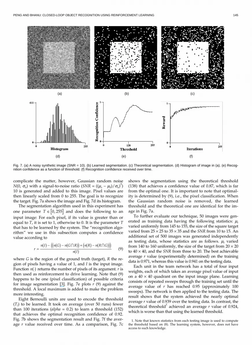
complicate the matter, however, Gaussian random noiseN(0, sn) with a signal-to-noise ratio (SNR = ((ms - mb)/sn)

2)

10 is generated and added to this image. Pixel values arethen linearly scaled from 0 to 255. The goal is to recognizethe target. Fig. 7a shows the image and Fig. 7d its histogram.

The segmentation algorithm used in this experiment has

one parameter T Π0 255, and does the following to an

input image: For each pixel, if its value is greater than orequal to T, it is set to 1, otherwise to 0. It is the parameter Tthat has to be learned by the system. The “recognition algo-rithm” we use in this subsection computes a confidencevalue according to

rn I n G n G R n R n R G

n I=

- - + -1 6 1 6 1 63 8 1 6 1 63 84 91 6

� � (9)

where G is the region of the ground truth (target), R the re-gion of pixels having a value of 1, and I is the input image.Function n ◊0 5 returns the number of pixels of its argument. r isthen used as reinforcement to drive learning. Note that (9)happens to be one (pixel classification) of possible criteriafor image segmentation [3]. Fig. 7e plots r (9) against thethreshold. A local maximum is added to make the problemmore interesting.

Eight Bernoulli units are used to encode the threshold(Tl) to be learned. It took on average (over 50 runs) fewerthan 100 iterations (alpha = 0.2) to learn a threshold (152)that achieves the optimal recognition confidence of 0.92.Fig. 7b shows the segmentation result and Fig. 7f the aver-age r value received over time. As a comparison, Fig. 7c

shows the segmentation using the theoretical threshold(138) that achieves a confidence value of 0.87, which is farfrom the optimal one. It is important to note that optimal-ity is determined by (9), i.e., the pixel classification. Whenthe Gaussian random noise is removed, the learnedthreshold and the theoretical one are identical for the im-age in Fig. 7a.

To further evaluate our technique, 50 images were gen-erated as training data having the following statistics: mt

varied uniformly from 145 to 155, the size of the square targetvaried from 25 ¥ 25 to 35 ¥ 35 and the SNR from 10 to 15. Anadditional set of 500 images was generated independentlyas testing data, whose statistics are as follows. mt variedfrom 140 to 160 uniformly, the size of the target from 20 ¥ 20to 40 ¥ 40, and the SNR from three to 20. The best achievableaverage r value (experimentally determined) on the trainingdata is 0.971, whereas this value is 0.941 on the testing data.

Each unit in the team network has a total of four inputweights, each of which takes an average pixel value of inputon a 40 ¥ 40 quadrant on the input image plane. Learningconsists of repeated sweeps through the training set until theaverage value of r has reached 0.95 (approximately 100sweeps). The network is then applied to the testing data. Theresult shows that the system achieved the nearly optimalaverage r value of 0.939 over the testing data. In contrast, thetheoretical threshold

1 achieved an average r value of 0.924,

which is worse than that using the learned threshold.

1. Note that known statistics from each testing image is used to computethe threshold based on (8). The learning system, however, does not haveaccess to such knowledge.

(a) (b) (c)

(d) (e) (f)

Fig. 7. (a) A noisy synthetic image (SNR = 10). (b) Learned segmentation. (c) Theoretical segmentation. (d) Histogram of image in (a). (e) Recog-nition confidence as a function of threshold. (f) Recognition confidence received over time.

146 IEEE TRANSACTIONS ON PATTERN ANALYSIS AND MACHINE INTELLIGENCE, VOL. 20, NO. 2, FEBRUARY 1998

These results show convincingly that the system can in-deed learn correct segmentation parameters and that whenimages are far from being ideal the learning system canactually outperform the theoretical method, at least forthose images presented here.

4.2 Evaluation on Real ImagesFor the color images the Phoenix algorithm [15] was chosenas the image segmentation component in our system be-cause it is a well-known method for the segmentation ofcolor images with a number of adjustable parameters. It hasbeen the subject of several PhD theses [19], [22]. Phoenixworks by splitting regions using histogram for color fea-tures. Appendix A provides a brief overview of the algo-rithm. Note that any segmentation algorithm with adjust-able parameters can be used in our approach.

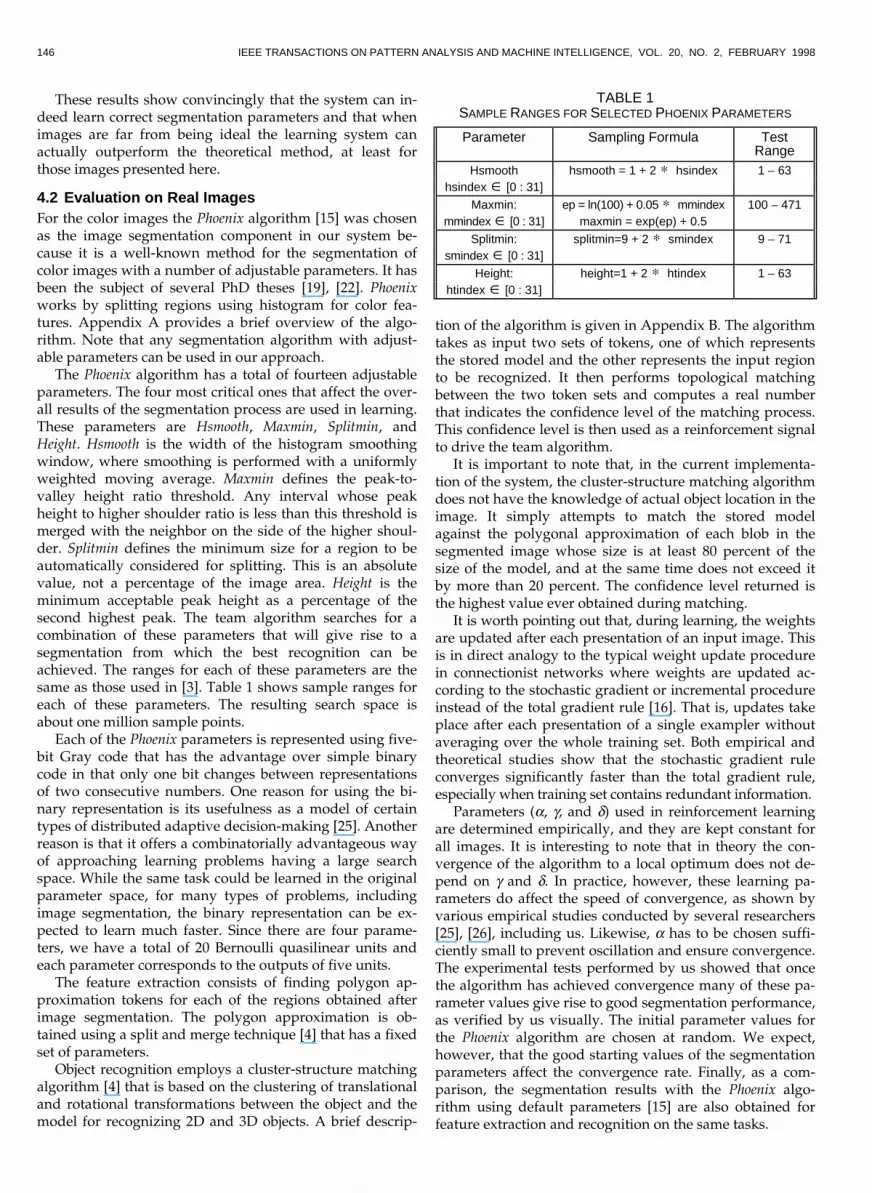
The Phoenix algorithm has a total of fourteen adjustableparameters. The four most critical ones that affect the over-all results of the segmentation process are used in learning.These parameters are Hsmooth, Maxmin, Splitmin, andHeight. Hsmooth is the width of the histogram smoothingwindow, where smoothing is performed with a uniformlyweighted moving average. Maxmin defines the peak-to-valley height ratio threshold. Any interval whose peakheight to higher shoulder ratio is less than this threshold ismerged with the neighbor on the side of the higher shoul-der. Splitmin defines the minimum size for a region to beautomatically considered for splitting. This is an absolutevalue, not a percentage of the image area. Height is theminimum acceptable peak height as a percentage of thesecond highest peak. The team algorithm searches for acombination of these parameters that will give rise to asegmentation from which the best recognition can beachieved. The ranges for each of these parameters are thesame as those used in [3]. Table 1 shows sample ranges foreach of these parameters. The resulting search space isabout one million sample points.

Each of the Phoenix parameters is represented using five-bit Gray code that has the advantage over simple binarycode in that only one bit changes between representationsof two consecutive numbers. One reason for using the bi-nary representation is its usefulness as a model of certaintypes of distributed adaptive decision-making [25]. Anotherreason is that it offers a combinatorially advantageous wayof approaching learning problems having a large searchspace. While the same task could be learned in the originalparameter space, for many types of problems, includingimage segmentation, the binary representation can be ex-pected to learn much faster. Since there are four parame-ters, we have a total of 20 Bernoulli quasilinear units andeach parameter corresponds to the outputs of five units.

The feature extraction consists of finding polygon ap-proximation tokens for each of the regions obtained afterimage segmentation. The polygon approximation is ob-tained using a split and merge technique [4] that has a fixedset of parameters.

Object recognition employs a cluster-structure matchingalgorithm [4] that is based on the clustering of translationaland rotational transformations between the object and themodel for recognizing 2D and 3D objects. A brief descrip-

tion of the algorithm is given in Appendix B. The algorithmtakes as input two sets of tokens, one of which representsthe stored model and the other represents the input regionto be recognized. It then performs topological matchingbetween the two token sets and computes a real numberthat indicates the confidence level of the matching process.This confidence level is then used as a reinforcement signalto drive the team algorithm.

It is important to note that, in the current implementa-tion of the system, the cluster-structure matching algorithmdoes not have the knowledge of actual object location in theimage. It simply attempts to match the stored modelagainst the polygonal approximation of each blob in thesegmented image whose size is at least 80 percent of thesize of the model, and at the same time does not exceed itby more than 20 percent. The confidence level returned isthe highest value ever obtained during matching.

It is worth pointing out that, during learning, the weightsare updated after each presentation of an input image. Thisis in direct analogy to the typical weight update procedurein connectionist networks where weights are updated ac-cording to the stochastic gradient or incremental procedureinstead of the total gradient rule [16]. That is, updates takeplace after each presentation of a single exampler withoutaveraging over the whole training set. Both empirical andtheoretical studies show that the stochastic gradient ruleconverges significantly faster than the total gradient rule,especially when training set contains redundant information.

Parameters (a, g, and d) used in reinforcement learningare determined empirically, and they are kept constant forall images. It is interesting to note that in theory the con-vergence of the algorithm to a local optimum does not de-pend on g and d. In practice, however, these learning pa-rameters do affect the speed of convergence, as shown byvarious empirical studies conducted by several researchers[25], [26], including us. Likewise, a has to be chosen suffi-ciently small to prevent oscillation and ensure convergence.The experimental tests performed by us showed that oncethe algorithm has achieved convergence many of these pa-rameter values give rise to good segmentation performance,as verified by us visually. The initial parameter values forthe Phoenix algorithm are chosen at random. We expect,however, that the good starting values of the segmentationparameters affect the convergence rate. Finally, as a com-parison, the segmentation results with the Phoenix algo-rithm using default parameters [15] are also obtained forfeature extraction and recognition on the same tasks.

TABLE 1SAMPLE RANGES FOR SELECTED PHOENIX PARAMETERS

Parameter Sampling Formula TestRange

Hsmooth hsmooth = 1 + 2 * hsindex 1 - 63hsindex Π[0 : 31]

Maxmin: ep = ln(100) + 0.05 * mmindex 100 - 471mmindex Π[0 : 31] maxmin = exp(ep) + 0.5

Splitmin: splitmin=9 + 2 * smindex 9 - 71smindex Π[0 : 31]

Height: height=1 + 2 * htindex 1 - 63htindex Π[0 : 31]

PENG AND BHANU: CLOSED-LOOP OBJECT RECOGNITION USING REINFORCEMENT LEARNING 147

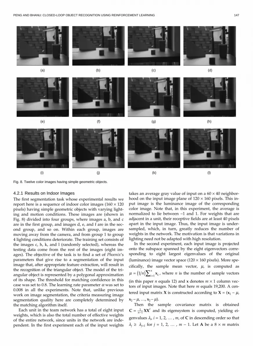
4.2.1 Results on Indoor ImagesThe first segmentation task whose experimental results wereport here is a sequence of indoor color images (160 ¥ 120pixels) having simple geometric objects with varying light-ing and motion conditions. These images are (shown inFig. 8) divided into four groups, where images a, b, and care in the first group, and images d, e, and f are in the sec-ond group, and so on. Within each group, images aremoving away from the camera, and from group 1 to group4 lighting conditions deteriorate. The training set consists ofthe images c, h, k, and l (randomly selected), whereas thetesting data come from the rest of the images (eight im-ages). The objective of the task is to find a set of Phoenix’sparameters that give rise to a segmentation of the inputimage that, after appropriate feature extraction, will result inthe recognition of the triangular object. The model of the tri-angular object is represented by a polygonal approximationof its shape. The threshold for matching confidence in thiscase was set to 0.8. The learning rate parameter a was set to0.008 in all the experiments. Note that, unlike previouswork on image segmentation, the criteria measuring imagesegmentation quality here are completely determined bythe matching algorithm itself.

Each unit in the team network has a total of eight inputweights, which is also the total number of effective weightsof the entire network, since units in the network are inde-pendent. In the first experiment each of the input weights

takes an average gray value of input on a 60 ¥ 40 neighbor-hood on the input image plane of 120 ¥ 160 pixels. This in-put image is the luminance image of the correspondingcolor image. Note that, in this experiment, the average isnormalized to lie between -1 and 1. For weights that areadjacent in a unit, their receptive fields are at least 40 pixelsapart in the input image. Thus, the input image is under-sampled, which, in turn, greatly reduces the number ofweights in the network. The motivation is that variations inlighting need not be adapted with high resolution.

In the second experiment, each input image is projectedonto the subspace spanned by the eight eigenvectors corre-sponding to eight largest eigenvalues of the original

(luminance) image vector space (120 ¥ 160 pixels). More spe-

cifically, the sample mean vector, m, is computed as

m ==Â1

1n

i

n2 7 xi , where n is the number of sample vectors

(in this paper n equals 12) and x denotes m ¥ 1 column vec-tors of input images. Note that here m equals 19,200. A cen-

tered input matrix X is constructed according to X = (x1 - m,

x2 - m, …, x2 - m).

Then the sample covariance matrix is obtained

C XX=-1

1nt and its eigensystem is computed, yielding ei-

genvalues li, i = 1, 2, … , m, of C in descending order so that

lj ≥ lj+1 for j = 1, 2, … , m - 1. Let A be a 8 ¥ m matrix

(a) (b) (c) (d)

(e) (f) (g) (h)

(i) (j) (k) (l)

Fig. 8. Twelve color images having simple geometric objects.

148 IEEE TRANSACTIONS ON PATTERN ANALYSIS AND MACHINE INTELLIGENCE, VOL. 20, NO. 2, FEBRUARY 1998

whose rows are formed from the eigenvectors of C, orderedso that the first row of A is the eigenvector correspondingto the largest eigenvalue, and the last row is the eigenvectorcorresponding to the eighth largest eigenvalue. Then newinputs are computed according to z = Ax where z denotes 8

¥ 1 column vectors. These inputs are normalized to lie be-

tween -1 and 1. Our goal is to see which experiment canoffer better performance. It turns out that the second ex-periment performed slightly better than the first one, as canbe seen below (Figs. 9 and 10). Note that, unless stated oth-erwise, all the figures in this section are obtained under thecondition that the system takes inputs from the subspacespanned by the first eight eigenvectors (major axes) corre-sponding to the eight largest eigenvalues of C.

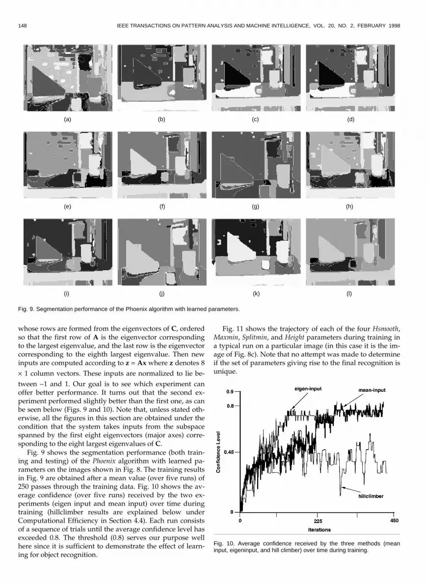
Fig. 9 shows the segmentation performance (both train-ing and testing) of the Phoenix algorithm with learned pa-rameters on the images shown in Fig. 8. The training resultsin Fig. 9 are obtained after a mean value (over five runs) of250 passes through the training data. Fig. 10 shows the av-erage confidence (over five runs) received by the two ex-periments (eigen input and mean input) over time duringtraining (hillclimber results are explained below underComputational Efficiency in Section 4.4). Each run consistsof a sequence of trials until the average confidence level hasexceeded 0.8. The threshold (0.8) serves our purpose wellhere since it is sufficient to demonstrate the effect of learn-ing for object recognition.

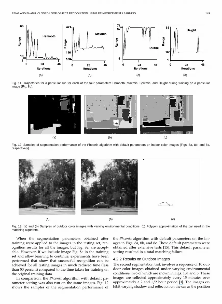
Fig. 11 shows the trajectory of each of the four Hsmooth,Maxmin, Splitmin, and Height parameters during training ina typical run on a particular image (in this case it is the im-age of Fig. 8c). Note that no attempt was made to determineif the set of parameters giving rise to the final recognition isunique.

(a) (b) (c) (d)

(e) (f) (g) (h)

(i) (j) (k) (l)

Fig. 9. Segmentation performance of the Phoenix algorithm with learned parameters.

Fig. 10. Average confidence received by the three methods (meaninput, eigeninput, and hill climber) over time during training.

PENG AND BHANU: CLOSED-LOOP OBJECT RECOGNITION USING REINFORCEMENT LEARNING 149

When the segmentation parameters obtained aftertraining were applied to the images in the testing set, rec-ognition results for all the images, but Fig. 8e, are accept-able. However, if we include image Fig. 8e in the trainingset and allow learning to continue, experiments have beenperformed that show that successful recognition can beachieved for all testing images in much reduced time (lessthan 50 percent) compared to the time taken for training onthe original training data.

In comparison, the Phoenix algorithm with default pa-rameter setting was also run on the same images. Fig. 12shows the samples of the segmentation performance of

the Phoenix algorithm with default parameters on the im-ages in Figs. 8a, 8b, and 8c. These default parameters wereobtained after extensive tests [15]. This default parametersetting resulted in a total matching failure.

4.2.2 Results on Outdoor ImagesThe second segmentation task involves a sequence of 10 out-door color images obtained under varying environmentalconditions, two of which are shown in Figs. 13a and b. Theseimages are collected approximately every 15 minutes overapproximately a 2 and 1/2 hour period [3]. The images ex-hibit varying shadow and reflection on the car as the position

(a) (b) (c) (d)

Fig. 11. Trajectories for a particular run for each of the four parameters Hsmooth, Maxmin, Splitmin, and Height during training on a particularimage (Fig. 8g).

(a) (b) (c)

Fig. 12. Samples of segmentation performance of the Phoenix algorithm with default parameters on indoor color images (Figs. 8a, 8b, and 8c,respectively).

(a) (b) (c)

Fig. 13. (a) and (b) Samples of outdoor color images with varying environmental conditions. (c) Polygon approximation of the car used in thematching algorithm.

150 IEEE TRANSACTIONS ON PATTERN ANALYSIS AND MACHINE INTELLIGENCE, VOL. 20, NO. 2, FEBRUARY 1998

of the sun changed and clouds came in and out the field ofview of the camera that had auto iris adjustment turned on.The overall goal is to recognize the car in the image. Theoriginal images are digitized at 480 ¥ 480 pixels in size andare then subsampled to produce 120 ¥ 120 pixel images. Fiveof these odd-numbered images are used as training data andfive even-numbered images as testing data.

Similar to the team network for the indoor images, eachunit here has a total of nine input weights, each of whichtakes an average gray value of input on a 40 ¥ 40 neighbor-hood on the input image plane of 120 ¥ 120 pixels. Theseaverages are normalized to lie between -1 and 1. Polygonalapproximation of the car shown in Fig. 13c is used as themodel in the cluster-structure matching algorithm. It wasextracted manually in an interactive session from the firstframe in the sequence.

Fig. 14 shows a sequence of segmentations for frame 1with Phoenix’s parameters sampled at iterations 20, 30, 40,50, 60, and 74 in a particular run during training, and corre-sponding parameter values at each of these intervals areshown in Table 2. Note that Fig. 14f shows the final seg-mentation result when the highest confidence matching hasbeen achieved. The threshold for acceptable matching con-fidence is set at 80 percent.

Figs. 15a and b show the Phoenix segmentation perform-ance on two testing images (frames 2 and 4) with learnedparameters obtained after training on frames 1, 3, 5, 7, and9. For frame 2, the matching is acceptable. However, forframe 4, the result is not acceptable, and learning is to beperformed similar to the indoor examples for the adapta-tion of parameters.

Finally, Figs. 15c and d show the samples of perform-ance of Phoenix with default parameters on the outdoorcolor images shown in Fig. 13. Note that these segmentationresults are totally unacceptable.

4.3 Evaluation on a Large Simulated Data SetThe simulated data experiment allows us to examine howthe system will behave with a large data set. We assume thefunction, F, representing segmentation, feature extractionand model matching components shown in Fig. 2, is given by

F Fk

kp px x0 5 0 5=

=

Â0

3

, (10)

and

F n x pki i

i kn

k n

p x1 6 4 91 6

= - -

= +

+

’2 5 14 1

1 4

. . (11)

where p Π{0, 1}n is a constant. F is a mapping from the n-

dimensional hypercube {0, 1}n into the real numbers, where

n = 20. Each point x in its domain is an n-dimensional bitvector.

TABLE 2CHANGES OF PARAMETER VALUES DURING TRAINING

Iteration Hsmooth Maxmin Splitmin Height 20 53 135 55 58

30 17 142 39 42

40 21 105 43 24

50 1 165 51 42

60 1 135 19 62

74 1 300 55 64

(a) (b) (c)

(d) (e) (f)

Fig. 14. Sequence of segmentations of the first frame during training.

PENG AND BHANU: CLOSED-LOOP OBJECT RECOGNITION USING REINFORCEMENT LEARNING 151

The function Fp(x) is computed as follows: Divide the 20bits into four equal-sized groups. For each group, computea score which is 2.5 n if all the bits in that group are thesame as those in p and is 0 otherwise. Then Fp(x) is the sumof these four scores. This function has a global maximum of200 at p. It also has very large plateaus over which thefunction is constant. These plateaus will confound any my-opic hillclimber.

In terms of the vision system described in the paper, xcorresponds to the encoding of segmentation parametersand Fp represents in abstract terms the matching confidenceresulting from applying Phoenix with x to a given inputimage p.

Note that since the precise nature of the function (10) to beoptimized is known, we can more reliably predict thestrengths and limitations of the system. In this experiment, pis randomly generated uniformly from {0, 1}

n. Then, 2,000

data points whose Hamming distance to p is at most fourare randomly generated from a distribution such that 80percent of the data points are produced by perturbing thefirst 10 bits of p, 10 percent by the first 15 bits, and the re-maining 10 percent by the entire 20 bits. Conceptually, eachof these data points may be viewed to simulate the seg-mentation parameter values for an image that will give riseto the best possible recognition result for the image.

Out of these 2,000 data points, 500 are randomly selectedas training data. The remaining 1,500 data points as testingdata. As in the real data experiments described above(Section 4.2), 15 normalized eigenfeatures are computed torepresent these data. Thus, there are 20 Bernoulli units,each of which has 15 input lines that encode a particularpattern to be searched for.

Training consists of repeated sweeps through the train-ing set until the average value of F has reached 190, whichis about 95 percent of the optimal value of 200 (see (10)). Anadded benefit is that it prevents the system from overfittingthe data, resulting in better generalization. The result showsthat after about 5,000 sweeps through the training data, thesystem achieved an average value of 180 over 90 percent ofthe testing data and an average value of 170 over the entiretesting data. Further examination revealed that the majorityof those testing data whose value is less than 180 comefrom 20 bit perturbation to p. These data were least repre-sented, and, therefore, resulted in relatively not-so-goodperformance. This generalization characteristic is typical inconnectionist networks. These results demonstrate that the

algorithm can be expected to perform reasonably well onlarge data sets in large problem domains.

4.4 Computational EfficiencyThe computational efficiency of the system should beevaluated against other systems having similar operatingcharacteristics. Currently there is no similar system in thecomputer vision field that directly uses recognition result asa feedback to drive learning for image segmentation. Thus,as a comparison we applied a stochastic hillclimber to thesame indoor images used for the experiments described inthe above (Section 4.2). We first applied the K-Means algo-rithm [17] to the eigenfeatures to determine K centers,where K = 4 in this experiment. Then four images that areclosest to the four centers are used as training data. Thereare, therefore, four sets of Phoenix parameters, each ofwhich is associated with a particular center. Again, 20 bitsare used to encode these Phoenix parameters. For a givenimage, generalization is made by searching for the nearestcluster center and then applying the set of Phoenix parame-ters associated with the cluster.

In the beginning, the hillclimber occasionally movesalong directions that are not very promising. However, assearch continues the probability of downhill movement isreduced. The annealing schedule (a schedule that reducesthe probability of downhill movement) used in this experi-ment is an inverse function of the number of iterations. It isimportant to note that if each dimension of the 20 dimen-sion input space at every iteration has to be examined toestimate the gradient, the amount of computation requiredwould be prohibitive. Instead, we randomly perturb threedimensions (where each dimension is equally likely to beselected) for each parameter set to move up the gradient.Thus, the amount of computation is three times of that re-quired by the reinforcement learning system at each itera-tion. The decision of where to look next critically influencesthe computational efficiency of the optimization process.Like the reinforcement learning method, however, a priorigradient information is not available. It has to be estimatedby sampling the search space. The average results (labeledas “hill-climber”) are shown in Fig. 10. A comparison ofthese results (Fig. 10) clearly demonstrates that the rein-forcement learning system performed significantly betterthan the stochastic hillclimber, despite the fact that it tookmore computation time at every iteration.

(a) (b) (c) (d)

Fig. 15. (a) and (b) Segmentation performance of the Phoenix algorithm on two testing images (frames 2 and 4) with learned parameters. (c) and(d) Samples of segmentation performance of the Phoenix algorithm with default parameters on the two images shown in Fig. 13.

152 IEEE TRANSACTIONS ON PATTERN ANALYSIS AND MACHINE INTELLIGENCE, VOL. 20, NO. 2, FEBRUARY 1998

5 CONCLUSIONS

Our choice of the team architecture is motivated by its sim-plicity and its generality as a representation scheme. Whatkind of problems an architecture can represent is to be de-termined experimentally and theoretically. In particular,one explanation for the successful results from the archi-tecture presented in this paper is that the images used ex-hibit well-behaved smoothness, that is, similar images infeature space require similar parameters for segmentation.We believe that this is true in general. In addition, deter-mining how close an architecture can approximate an un-known mapping is a classical problem, and many criteriahave been proposed, such as the Probably ApproximatelyCorrect (PAC) learning theory and the Minimum Descrip-tion Length (MDL) measure. It is in general an ill-posedproblem. In practice, however, it is often determined ex-perimentally through cross-validation. The architecturepresented in this paper seemed to approximate the un-known mappings sufficiently well, for nearly optimal per-formance has been achieved. These results shed light on thelarge potential of the proposed architecture, and present abasis for additional experiments to determine the scope ofapplicability of the architecture beyond the current problemreported in this paper.

The key contribution of the paper is the general frame-work for the usage of reinforcement learning in a model-based object recognition system. Our investigation into re-inforcement learning-based object recognition shows con-vincingly that a robust and adaptive system can be devel-oped that autonomously determines the criteria for seg-mentation of the input images and selects useful featuresthat result in a system with high recognition accuracy whenapplied to unseen images. Note that the performance of anylearning-based computer vision system depends on thevision algorithms that are used, e.g., the Phoenix algorithmused in this paper for the segmentation of color images.Future research will address extensions for enlarging thescope of the approach to encompass closed-loop 3D objectrecognition and problems in active vision where reinforce-ment learning could be extremely useful. Furthermore, in-corporation of “delayed” reinforcement learning couldadequately address the inherent multilevel nature of visionsystems [20].

APPENDIX A: THE PHOENIX SEGMENTATIONALGORITHM

The Phoenix image segmentation algorithm is based on arecursive region splitting technique [15]. It uses informationfrom the histograms of the red, green, and blue image com-ponents to split regions in the image into smaller sub-regions on the basis of a peak/valley analysis of each histo-gram. An input image typically consists of red, green, andblue image planes, although monochrome images, textureplanes, and other pixel-oriented data may also be used.Each plane is called a feature or feature plane.

Fig. 16 shows a conceptual description of the Phoenixsegmentation process. It begins with the entire image as asingle region. It then fetches this region and attempts tosegment it using histogram and spatial analyses. If it suc-

ceeds, the program fetches each of the new regions in turnand attempts to segment them. The process terminateswhen no region can be further segmented.

The histogram analysis phase computes a histogram foreach feature plane, analyzes it and selects thresholds orhistogram cutpoints that are likely to identify significanthomogeneous regions in the image. A set of thresholds forone feature is called an interval set. During the analysis, ahistogram is first smoothed with an unweighted windowaverage, where the window width is hsmooth. It is then bro-ken into intervals such that each contains a peak and two“shoulders.” A series of heuristics is applied to eliminatenoise peaks. When an interval is removed, it is merged withthe neighbor sharing the higher of its two shoulders. Split-min is the minimum area for a region to be automaticallyconsidered for splitting.

Two tests determine if an interval should be retained.First, the ratio of peak height to the height of its highershoulder must be greater than or equal to the maxminthreshold. Second, the interval area must be larger than anabsolute threshold and the relative area, percent of the totalhistogram area. The second highest peak can now be found,and peaks lower than the height percent of this peak aremerged. The lowest valley is then determined, and any in-terval whose right shoulder is higher than absmin (Phoenix’sparameter) times this valley is merged with its right neigh-bor. Finally, only intsmax (Phoenix’s parameter) intervals areretained by repeatedly merging intervals with low peak-to-shoulder ratio.

The spatial analysis selects the most promising intervalsets, thresholds the corresponding feature planes, and ex-tracts connected components for spatial evaluation. Thefeature and the interval set providing the best segmentation(the least noise area) are accepted as the segmentation fea-ture and the thresholds.

The histogram cutpoints are now applied to the featureplane as intensity thresholds and connected componentsare extracted. After each feature has been evaluated, theone producing the least total noise area is accepted as thesegmentation feature. If no suitable feature is found, theoriginal region is declared terminal. Otherwise, the valid

Fig. 16. Conceptual diagram of the Phoenix segmentation algorithm.

PENG AND BHANU: CLOSED-LOOP OBJECT RECOGNITION USING REINFORCEMENT LEARNING 153

patches, merged with the noise patches, are converted tonew regions and added to the segmentation record. In ei-ther case, a new segmentation pass is scheduled. For addi-tional details, see [15].

APPENDIX B: THE CLUSTER-STRUCTUREALGORITHM

The cluster-structure algorithm can be divided into the fol-lowing main steps:

1) Determine Disparity Matrix,2) Initial Clustering,3) Sequencing,4) Final Clustering,5) Transform Computation.

The algorithm first computes the disparity matrix. It deter-mines the segment length of each line and the angles be-tween successive lines from the set of vertices for the modeland the image input to the program. At this point, everysegment in the model will be compared against every seg-ment in the image. If segment lengths and successor anglesare compatible, the algorithm computes the rotational andtranslational disparity between pairs of segments. Thesevalues are stored in the disparity matrix and are indexed bythe segment numbers in the model and the image. The al-gorithm continues until all segments have been compared.It then computes the range of rotational and translationalvalues present in the matrix, and normalizes them overtheir appropriate range.

The initial clustering determines clusters from the nor-malized values in the disparity matrix. At each step, theprogram clusters all of the samples, recomputes the newcluster centers, and continues until none of the cluster cen-ters change their positions. The program then selects thecluster having the largest number of samples. Also selectedare the clusters that are within 20 percent of the largest one.Each cluster is considered separately and the final trans-form comes from the cluster that yields the highest confi-dence level.

The sequencing step uses the samples in the currentcluster to find all sequences in the samples. This providesthe critical structural information. Samples that are notplaced in any sequence are discarded. The program alsoremoves sequences that have a segment count of less thanthree (three segments comprise the basic local shape struc-ture). It then computes the rotational and translation aver-ages of each sequence that has been located.

Using the sequences and the sequence averages, the finalclustering step clusters these values to find those sequencesthat lead to the same rotational and translational results.This is achieved by using the iterative technique of cluster-ing, evaluating, clustering, etc. The program then selects thecluster that contains the largest number of sequences andpasses this cluster to the final step.

The final step of the algorithm computes the confidencelevel of the transformation determined by each cluster. Thecluster having the highest confidence level is selected as thefinal transformation cluster. It assembles the set of matchedsegments in the sequences in this cluster. The final output

of the program is the rotation and the vertical and hori-zontal translation necessary to locate the model within theimage. The program also produces a confidence level indi-cating the likelihood that the final matching is correct. Forfurther details, see [4].

ACKNOWLEDGMENTS

This work was supported by DARPA/AFOSR grantsF49620-97-1-0184 and F49620-95-1-0424. The contents of theinformation do not necessarily reflect the position or thepolicy of the U.S. Government.

REFERENCES

[1] A.G. Barto, R.S. Sutton, and C.J.C.H. Watkins, “Learning andSequential Decision Making,” COINS Technical Report 89-95,Dept. of Computer and Information Science, Univ. of Mass., Am-herst, Mass., 1989.

[2] B. Bhanu and T. Jones, “Image Understanding Research forAutomatic Target Recognition,” Proc. DARPA Image Understand-ing Workshop, pp. 249-259, 1992.

[3] B. Bhanu and S. Lee, Genetic Learning for Adaptive Image Segmenta-tion. Boston, Mass.: Kluwer Academic Publishers, 1994.

[4] B. Bhanu and J. Ming, “Recognition of Occluded Objects: A Clus-ter-Structure Algorithm,” Pattern Recognition, vol. 20, no. 2, pp.199-211, 1987.

[5] B. Bhanu, S. Lee, and S. Das, “Adaptive Image Segmentation Us-ing Genetic and Hybrid Search Methods,” IEEE Trans. Aerospaceand Electronic Systems, vol. 31, no. 4, pp. 1,268-1,291, Oct. 1995.

[6] B. Bhanu, S. Lee, and J. Ming, “Adaptive Image SegmentationUsing a Genetic Algorithm,” IEEE Trans. Systems, Man, and Cyber-netics, vol. 25, no. 12, pp. 1,543-1,567, Dec. 1995.

[7] D. Chapman, “Intermediate Vision: Architecture, Implementa-tion, and Use,” Cognitive Science, vol. 16, pp. 491-537, 1992.

[8] R.T. Chin and C.R. Dyer, “Model-Based Recognition in RobotVision,” ACM Computing Surveys, pp. 67-108, Mar. 1994.

[9] M.A. Fischler, “On the Representation of Natural Scenes,” Com-puter Vision Systems, A.R. Hanson and E.M. Riseman, eds. NewYork: Academic Press, 1978.

[10] K. Fukushima, S. Miyake, and T. Ito, “Neocognition: A NeuralNetwork Model for a Mechanism of Visual Pattern Recognition,”IEEE Trans. Systems, Man, and Cybernetics, vol. 13, no. 5, pp. 826-834, Sept. 1983.

[11] D.E. Goldberg and J.H. Holland, Special Issue on Genetic Algo-rithms, Machine Learning, 2/3, 1988.

[12] R.C. Gonzalez and P. Wintz, Digital Image Processing. Addison-Wesley Publishing Co., 1977.

[13] R.M. Haralick and L.G. Shapiro, “Image Segmentation Tech-niques,” Computer Vision, Graphics, and Image Processing, vol. 29,pp. 100-132, 1985.

[14] H.G. John, R. Kohavi, and K. Pfleger, “Irrelevant Features and theSubet Selection Problem,” Proc. 11th Int’l Conf. Machine Learning,pp. 121-129, 1994.

[15] K. Laws, “The Phoenix Image Segmentation System: Descriptionand Evaluation,” SRI Int’l Tech. Rep. TR289, Dec. 1982.

[16] Y. LeCun, B. Boser, J.S. Denker, D. Henderson, R.E. Howard, W.Hubbard, and L.D. Jackel, “Backpropagation Applied to Hand-written Zip Code Recognition,” Neural Computation, vol. 1, pp. 541-551, 1989.

[17] J.L. Marroquin and F. Girosi, “Some Extensions of the K-MeansAlgorithm for Image Segmentation and Pattern Classification,”A.I. Memo No. 1390, MIT AI Lab, 1993.

[18] K.S. Narendra and M.A.L. Thathatchar, Learning Automata: AnIntroduction. Englewood Cliffs, N.J.: Prentice Hall, 1989.

[19] R. Ohlander, K. Price, and D. R. Reddy, “Picture SegmentationUsing a Recursive Region Splitting Method,” Computer Graphicsand Image Processing, vol. 8, pp. 313-333, 1978.

[20] J. Peng and B. Bhanu, “Delayed Reinforcement Learning forClosed-Loop Object Recognition,” Proc. DARPA Image Under-standing Workshop, pp. 1,429-1,435, Feb. 1996.

154 IEEE TRANSACTIONS ON PATTERN ANALYSIS AND MACHINE INTELLIGENCE, VOL. 20, NO. 2, FEBRUARY 1998

[21] V. Ramesh, “Performance Characterization of Image Under-standing Algorithms,” PhD Thesis, Dept. of Electrical Eng., Univ.of Washington, Seattle, Washington, 1995.

[22] S. Shafer and T. Kanade, “Recursive Region Segmentation byAnalysis of Histograms,” Proc. IEEE Int’l Conf. Acoustics, Speech,and Signal Processing, pp. 1,166-1,171, 1982.

[23] P. Suetens, P. Fua, and A.J. Hanson, “Computational Strategiesfor Object Recognition,” ACM Computing Surveys, vol. 24, no. 1,pp. 5-59, 1992.

[24] S. Wang and T. Binford, “Local Step Edge Estimation—A NewAlgorithm, Statistical Model, and Performance Evaluation,” Proc.ARPA Image Understanding Workshop, pp. 1,063-1,070, Apr. 1993.

[25] R.J. Williams, “Simple Statistical Gradient-Following Algorithmsfor Connectionist Reinforcement Learning,” Machine Learning,vol. 8, pp. 229-256, 1992.

[26] R.J. Williams and J. Peng, “Function Optimization Using Connec-tionist Reinforcement Learning Algorithms,” Connection Science,vol. 3, no. 3, 1991.

Jing Peng received the BS degree in computerscience from the Beijing Institute of Aeronauticsand Astronautics, Beijing, China. He also re-ceived the MA degree in computer science fromBrandeis University and the PhD degree in com-puter science from Northeastern University,Boston, Mass. Recently, he has been a researchscientist with Visualization and Intelligent Sys-tems Laboratory at the University of California atRiverside. Dr. Peng’s research interests includemachine learning, computer vision, image data-

bases, and learning and vision applications.

Bir Bhanu received the SM and EE degrees inelectrical engineering and computer sciencefrom the Massachusetts Institute of Technology,Cambridge, Massachusetts, the PhD degree inelectrical engineering from the Image ProcessingInstitute, University of Southern California, LosAngeles, and the MBA degree from the Univer-sity of California, Irvine. He also received the BSdegree (with Honors) in electronics engineeringfrom the Institute of Technology, BHU, Varanasi,India, and the ME degree (with Distinction) in

electronics engineering from Birla Institute of Technology and Science,Pilani, India.

Since 1991, he has been a professor of electrical engineering andcomputer science and director of Visualization and Intelligent SystemsLaboratory at the University of California, Riverside. Previously, he wasa Senior Honeywell Fellow at Honeywell Systems and Research Cen-ter, Minneapolis, Minnesota. He has been on the faculty of the De-partment of Computer Science at the University of Utah, Salt Lake City,and has also worked with Ford Aerospace and Communications Cor-poration, INRIA-France, and IBM San Jose Research Laboratory,California. He has been the principal investigator of various programsfor DARPA, NASA, the U.S. National Science Foundation, AFOSR,ARO, and other agencies and industries in the areas of learning andvision, image understanding, pattern recognition, target recognition,navigation, image databases, and machine vision applications. He isthe coauthor of the books Computational Learning for Adaptive Com-puter Vision (Plenum, forthcoming), Genetic Learning for AdaptiveImage Segmentation (Kluwer, 1994), and Qualitative Motion Under-standing (Kluwer 1992). He received an outstanding paper award fromthe Pattern Recognition Society. He has also received industrialawards for technical excellence, outstanding contributions, and teamefforts. He has been the guest editor of several IEEE transactions andjournals and is on the editorial board of various journals. He holds 10U.S. and international patents and has published more than 150 re-viewed technical publications in the areas of his interest. He was theGeneral Chair for the first IEEE Workshop on Applications of ComputerVision, Chair for the DARPA Image Understanding Workshop, andGeneral Chair for the IEEE Conference on Computer Vision and Pat-tern Recognition.

Dr. Bhanu is a Fellow of the IEEE and AAAS (American Associationfor the Advancement of Science). He is a member of ACM, AAAI,Sigma Xi, Pattern Recognition Society, and SPIE.