University of PennsylvaniaScholarlyCommons

Real-Time and Embedded Systems Lab (mLAB) School of Engineering and Applied Science

5-6-2015

Technical Report: Abstraction-Tree For Closed-loop Model Checking of Medical DevicesZhihao JiangUniversity of Pennsylvania, zhihaoj@seas.upenn.edu

Houssam AbbasUniversity of Pennsylvania, habbas@seas.upenn.edu

Pieter J. MostermanMathWorks, Pieter.Mosterman@mathworks.com

Rahul MangharamUniversity of Pennsylvania, rahulm@seas.upenn.edu

Follow this and additional works at: http://repository.upenn.edu/mlab_papers

Part of the Computer Engineering Commons, and the Electrical and Computer EngineeringCommons

This paper is posted at ScholarlyCommons. http://repository.upenn.edu/mlab_papers/73For more information, please contact repository@pobox.upenn.edu.

Recommended CitationZhihao Jiang, Houssam Abbas, Pieter J. Mosterman, and Rahul Mangharam, "Technical Report: Abstraction-Tree For Closed-loopModel Checking of Medical Devices", . May 2015.

Technical Report: Abstraction-Tree For Closed-loop Model Checking ofMedical Devices

DisciplinesComputer Engineering | Electrical and Computer Engineering

This technical report is available at ScholarlyCommons: http://repository.upenn.edu/mlab_papers/73

Abstraction Trees for Closed-Loop ModelChecking of Medical Devices?

Zhihao Jiang1, Houssam Abbas1, Pieter J. Mosterman2,3, and RahulMangharam1

1 Department of Electrical and Systems Engineering, University of Pennsylvania2 School of Computer Science, McGill University, Canada

3 MathWorks, USA

Abstract. This paper proposes a methodology for closed-loop model check-ing of medical devices, and illustrates it with a case study on implantablecardiac pacemakers. To evaluate the performance of a medical device onthe human body, a model of the device’s physiological environment must bedeveloped, and the closed-loop consisting of device (e.g., pacemaker) andenvironment (e.g., the human heart) is model-checked. Formal modeling ofthe environment and its application in model checking pose several chal-lenges that are addressed in this paper. Pacemakers should guarantee safeoperations across large varieties of heart conditions, which are representedby an incomplete set of timed automata models. A set of domain-specificabstraction rules are developed that can over-approximate the timing be-haviors of a heart model or a group of heart models, such that the newbehaviors introduced by abstraction are mostly physiologically meaningful.The rules serve as a systematic method to cover heart conditions that maynot be explicitly accounted for in the initial set of heart models. Closed-loopmodel checking is systematically performed using the heart models in theabstraction tree, to obtain the most concrete counter-example(s) that cor-respond to property violation. These counter-examples, along with theirphysiological context, are then presented to the physician to determinetheir physiological validity. The proposed methodology creates a separa-tion between steps requiring physiological domain expertise (model cre-ation and abstraction rules definition) and steps that can be automated(rule application, model checking, and abstraction refinement). While themethodology is illustrated for pacemaker verification, it is more broadlyapplicable to the verification of other medical devices.

1 Introduction

Implantable medical devices such as pacemakers are designed to improve physiolog-ical conditions with very little human intervention. Their ability to autonomouslyaffect the physiological state of the patient makes the medical devices safety-critical, and sufficient evidence for their safety and efficacy should be providedbefore the devices can be implanted in the patients. Medical devices increasinglyrely on software, and device function and their clinical performance can be affectedby seemingly minor changes to software. 4

? NSF CAREER 1253842, NSF MRI 1450342. This work was also supported by STAR-net, a Semiconductor Research Corporation program, sponsored by MARCO andDARPA.

4 In what follows, the word ‘device’ is used to refer to the software of the device.

2

Over the course of the past four decades, cardiac rhythm management devicessuch as pacemakers and implantable cardioverter defibrillators (ICD) have grownin complexity and now have more than 80,000 to 100,000 lines of software code [2].In 1996, 10% of all medical device recalls were caused by software-related issuesand this rose to 15% between 2003-2012 [8,19]. There is currently no standard fortesting, validating, and verifying the software for implantable medical devices.

There are two categories of device bugs: 1) the device may fail to conform toits specifications, that is, the prescription of how it should react to certain inputs.2) the device may fail to improve the conditions of the patient as promised, evenif it conforms to its specifications. The desired physiological conditions that theclosed-loop system should achieve are captured in the physiological requirements;for example, for a pacemaker, the heart rate should always be maintained abovea certain threshold.

Bugs in the first category (non-conformance to specification) can be detectedvia systematic and extensive open-loop testing in which a set of input sequencesis fed to the device, and its output is compared with the expected output. Bugs inthe second category (violation of physiological requirements), on the other hand,require the availability of the closed-loop system, which consists of the device andits environment. For instance, the pacemaker and the heart as its environment. Inthe medical device industry, closed-loop verification of the physiological require-ments is mostly performed in terms of clinical trials, in which the actual devices areimplanted in human subjects over an extended duration. Unfortunately, becauseof the extremely high cost of clinical trials ($0.30 million to $24.03 million [9].with cardiac devices closer to the higher end), the amount and variety of humansubjects during the clinical trials are limited, which reduces the opportunity tofind bugs. Moreover, clinical trials are often conducted at the final design stage.Fixing bugs at this stage is very costly.

Closed-loop model checking enables closed-loop evaluation of the physiologi-cal requirements at an earlier design stage, which requires formal model(s) of thephysiological environment. In closed-loop model checking, there is only one devicemodel. However there can be a large number of environmental conditions whichrequire different models to represent them. For instance, a heart with atrial flutterhas an additional conduction pathway that is not available in a healthy heart,causing fast atrial rate. The timing and structural differences should be distin-guished in corresponding heart models. A set of initial models of the environmentcan be constructed but the set is inherently incomplete because of the large num-ber of environment conditions and their combinations. As a result, performingmodel checking using every model in the set cannot ensure full coverage of theenvironmental conditions.

In this paper, domain-specific over-approximation rules are developed that pro-duce abstract models that not only cover explicitly modeled environment condi-tions, but also cover timing behaviors and conditions not modeled in the set ofinitial models. The abstract models can be then used for closed-loop model check-ing of the device model. If the closed-loop system satisfies a requirement, the deviceunder verification satisfies the requirement under environment conditions coveredby the abstract models. However, if the requirement is not satisfied, the modelchecker returns a counter-example. In device modeling, the counter-example isconsidered spurious if it can not be produced by the device. However in environ-

3

Bugs

Device

InitialAbstraction

PredicateAbstraction

ℎ𝑖𝑛𝑖𝑡

Refinement 1

Refinement NHeart

Condition 2

Spurious Counter-example 1

Spurious Counter-example N

HeartCondition 3

HeartCondition 1

Abstraction 1.2

Abstraction 1.1

Abstraction 2.1

HeartCondition x

ℎ1

ℎ1

ℎ2

Abstraction Tree of Environment Models

Closed-loopModel Checking

Abstraction

Refinement

Concretized counter-examples with Physiological context Physician(a) (b) Bugs

Pacemaker

1 2

3

Fig. 1. (a) Device modeling with CEGAR framework (b) Closed-loop model checkingwith environment abstraction tree.

ment modeling, even if the counter-example can not be produced by any of theinitial environment models, it might still be a physiologically valid behavior. Thusthe validity of a counter-example cannot be determined by refining the environ-ment model, but can untimately only be determined by domain experts.

Counter-examples returned from abstract models can be difficult to interpretby domain experts. One abstract counter-example could be produced by multiplephysiologically valid conditions, which causes ambiguity. Thus, a rigorous frame-work is necessary to balance the need to cover a wide range of environmental con-ditions and the need to provide counter-examples to the physicians within theirphysiological context.

Another challenge for closed-loop model checking of medical devices is theamount of domain expertise needed during: 1) physiological modeling, 2) modelabstraction and refinement, and 3) checking the validity of counter-examples. Thusthe framework must also allow non-domain experts to perform verification (item2 above), and establish ‘hand-off’ points where the results of verification can behanded back to the experts for interpretation.

1.1 Contributions

In this paper a framework is proposed for environment modeling in closed-loopmodel checking of medical device software. The cardiac pacemaker is used as anexample of applying this framework. An expandable set of timed-automata heartmodels are first developed to represent different physiological conditions (Fig. 1Marker 1). A set of domain-specific abstraction rules are then developed basedon physiological knowledge, which help ensure the physiological relevance of thebehaviors introduced into the abstract models (Fig. 1 Marker 2). Then the rulesare applied to the initial set of physiological models to obtain an abstraction tree,which will be used for closed-loop model checking of the pacemaker. A straightfor-ward search procedure is then used to conduct model checking using suitable heartmodels and return the most concrete and unambiguous counter-examples to thephysicians for analysis (Fig. 1 Marker 3). In this framework, physiological knowl-edge is only needed when constructing the initial model set and when analyzingcounter-examples. The application of the physiological abstraction rules and theverification procedure can be automated. The proposed method can potentiallybe generalized to other domains in which the device operates in a large variety ofenvironmental conditions.

4

1.2 Related Work

Counter-Example Guided Abstraction Refinement (CEGAR) [6] has been pro-posed to over-approximate the behaviors of the device using predicate abstraction(Fig. 1.(a)). CEGAR works well during device modeling, however, it cannot beapplied to environment modeling for two reasons: 1) predicate abstraction doesnot guarantee the validity of behaviors introduced into the model. In fact, fordevice modeling, all additional behaviors introduced into the abstract model arespurious. 2) the validity of a counter-example cannot be checked automatically asin device modeling.

Proof-based approach has also been applied to verify abstractions and refine-ments of pacemaker specification using Event-B [7]. However, the authors did nottake into account environment behaviors thus the framework cannot be used forverifying physiological requirements.

Physiological modeling of cardiac activities has been studied at different levelsfor different applications. In [20] the electrical activities of the heart are modeled inhigh spatial fidelity to study the mechanisms of cardiac arrhythmia. In [10] formalabstractions of cardiac tissue have been studied to reduce the complexity of theheart tissue model. However, these two models do not focus on the interactionwith the pacemaker, therefore cannot be used for closed-loop model checking. In[5] hybrid automata models of the heart has been used to capture the complexbeat-to-beat dynamics of the heart tissue. However the model cannot be used tocover behaviors of multiple heart conditions.

In previous work [13] a set of formal heart models covering various heart condi-tions at different abstraction levels were developed, and closed-loop model checkinghas been performed on models of implantable pacemakers. However, the physio-logical knowledge required during each step of closed-loop model checking preventsthe method to be practical.

2 Technical preliminaries

Timed automata [4] are an extension of finite automata with a finite set of real-valued clocks. A timed automaton G is a tuple 〈S, S0, Σ,X, inv,E〉, where S is afinite set of locations. S0 ⊂ S is the set of initial locations. Σ is the set of events.X is the set of clocks. inv is the set of invariants for clock constraints at eachlocation. E is the set of edges. Each edge is a tuple 〈s, σ, ψ, λ, s′〉 which consists ofa source location s, an event σ ∈ Σ, clock constraints ψ, λ as a set of clocks to bereset and the target location s′. For the clock variables X, the clock constraints Ψcan be inductively defined by Ψ := x⊥c‖Ψ1 ∧Ψ2, where ⊥ ∈ ≤,=,≥, and c ∈ N.

Semantics of Timed Automata A state of a timed automaton is a pair 〈s, v〉which contains the location s ∈ S and the valuation v : X → R for all clocks. Theset of all states is Ω. For all λ ⊆ X, v[λ := 0] denotes the valuation which setsall clocks x ∈ λ as zero and the rest of the clocks unchanged. For all t ∈ R, v + tdenotes the valuation which increases all the clock value by t. There are two kindsof transitions between states. The discrete transition happens when the condition

5

𝛿1

𝛿3

𝛿′𝛿2

𝑠𝑖𝑚Ω𝜔ℬ(𝑀)

ℬ(𝑀′)Ω′𝜔

ℬ(𝑆𝑦𝑠1)

ℬ(𝑆𝑦𝑠2)

ℬ(𝜑)ℬ 𝜑

Fig. 2. Two models Sys1, Sys2 are over-approximated by model M such thatSys1, Sys2 t M . M ′ time-simulates M such that M t M

′. For a property ϕ ifM ′ 6|= ϕ, δ′ is returned as counter-example. However, δ′ corresponds to 3 different be-haviors in the original behavior space: δ1 satisfies ϕ and is produced by Sys1, δ2 falsifiesϕ and is produced by Sys2, and δ3 falsifies ϕ and belongs to neither behavior space.

of an edge has been met. So we have:

〈s, σ, ψ, λ, s′〉 ∈ E, v |= ψ, v[λ := 0] |= inv(s′)⇒ (s, v)σ−→ (s′, v[λ := 0])

The timed transition happens when the timed automaton can stay in the samelocation for certain amount of time. We have:

τ ∈ R,∀τ ′ ≤ τ, v + τ ′ |= inv(s)⇒ (s, v)τ−→ (s, v + τ)

Observable Timed Simulation For two timed automata T 1 =⟨S1, S1

0 , Σ1, X1, inv1, E1

⟩and T 2 =

⟨S2, S2

0 , Σ2, X2, inv2, E2

⟩, Σo ⊆ Σ1 ∩ Σ2 is a set of observable events,

an observable timed simulation relation is a binary relation simo ⊆ Ω1×Ω2 whereΩ1 and Ω2 are sets of states of T 1 and T 2. We say T 2 simulates T 1 (T 1 t T 2) ifthe following conditions holds:

– Initial states correspondence: (⟨s10,0

⟩,⟨s20,0

⟩) ∈ simo

– Timed transition: For every (〈s1, v1〉 , 〈s2, v2〉) ∈ simo, if 〈s1, v1〉τ−→ 〈s1, v1 + τ〉,

there exists 〈s2, v2 + τ〉 such that 〈s2, v2〉τ−→ 〈s2, v2 + τ〉 and

(〈s1, v1 + τ〉 , 〈s2, v2 + τ〉) ∈ simo.

– Observable discrete transition: For every (〈s1, v1〉 , 〈s2, v2〉) ∈ simo, if 〈s1, v1〉σo−→

〈s′1, v′1〉, in which σo ∈ Σo, there exists 〈s′2, v′2〉 such that 〈s2, v2〉σo−→ 〈s′2, v′2〉

and (〈s′1, v′1〉 , 〈s′2, v′2〉) ∈ simo.

Observable timed-simulation can also be used to cover the behaviors of multiplemodels. A model M ′simulates models M1 and M2 if M1 t M ′ and M2 t M ′,which is denoted as M1,M2 t M ′.

A trace of a timed automaton M is a sequence δ with 〈s1, v1〉 · · · 〈sn, vn〉 such

that ∀i ∈ [1 · · ·n − 1], 〈si, vi〉α−→ 〈si+1, vi+1〉 ∈ E for α ∈ Σ ∪ R. The reachable

behavior space of M is denoted as B(M) ⊂ Ωω. For a timed-automata M ′ suchthat M t M ′, for every trace δ ∈ B(M), there exists a trace δ′ ∈ B(M ′) with〈s′1, v′1〉 · · · 〈s′n, v′n〉 such that ∀i ∈ [1, n − 1], 〈s′i, v′i〉 →

⟨s′i+1, v

′i+1

⟩∈ E′, and also

(〈si, vi〉 , 〈s′i, v′i〉) ∈ simo. We abuse the notation of simo and denote (δ, δ′) ∈ simo.M ′ has more behaviors than M , and we say that M ′ over-approximates M .

Validity of a counter-example: Certain properties are preserved in timedsimulation relation. For ϕ ∈ ATCTL∗, ifM t M ′, we haveM ′ |= ϕ⇒M |= ϕ [6].

6

Retro

t<=Tcond_max

Ante

t<=Tcond_max

Idle

t>Tcond_minAct_node_1!

t>Tcond_minAct_node_2!

Act_path_1?Act_path_2?

Act_path_2?

t=0

Act_path_1?

t=0

ERPt<=Terp_max

temp

Rest

t<=Trest_maxt>Trest_min

t=0

t>Terp_mint=0

Act_path!

Act_node?t=0

Refractory

Time

V out

ERP Rest Rest

ERP Rest Rest

(b) Node Automaton N0

(c) Path Automaton P0

SALA

(d) Graph of timed automata(a)

1 2

RA

AV His

RV

RVA

LVA

LV

Fig. 3. (a) Action potential for a heart tissue and its tissue nearby (dashed). (b) Nodeautomaton. (c) Path automaton. (d) An example model of the heart consist of a networkof node and path automata. The nodes are labeled with the name of the correspondingphysiological structures.

However, in general M ′ 6|= ϕ⇒M 6|= ϕ does not hold. Violations of ATCTL yieldcounter-examples and the validity of which need to be checked. For two models suchthat M t M ′, δ′ ∈ B(M ′) is spurious if 6 ∃δ ∈ B(M) s.t. 〈δ, δ′〉 ∈ simo. However,for environment models such that M1,M2, ...Mn t M ′, and an execution δ′ ∈B(M ′), the following condition is enough to prove δ′ is spurious, but not necessarilyinvalid.

∀i 6 ∃δ ∈ B(Mi) s.t. 〈δ, δ′〉 ∈ simo

Since there may be a valid environment model Mc 6∈ M1,M2, ...Mn andB(Mc) ⊂ B(M ′) and δ′ ∈ B(Mc). It is thus up to the domain experts to determinethe validity of the counter-example.

3 Formal Models of the Environment

To perform closed-loop model checking of medical devices, formal models of theirphysiological environment are needed to represent different physiological condi-tions the devices may encounter. In this section, timed-automata [4] models ofthe human heart are developed as the environment model for implantable pace-maker [13,15]. Physiological requirements are formalized with monitors andATCTL∗

formula [3]. Model checking can then be performed on the closed-loop system inmodel checker UPPAAL [18].

3.1 Timed Automata Models of the Heart

At cellular level, a heart tissue can be activated by external voltage. Certain tissuealso has capability to self-activate, which contribute to natural heart beats. Onceactivated (Marker 1 in Fig. 3), the voltage outside the tissue changes over time,which is referred to as Action Potential (Fig. 3.(a)). The action potential can bedivided into two functional timing periods: The Effective Refractory Period (ERP),during which the tissue cannot be triggered by another activation; and the Restperiod, during which the tissue can be activated and at the end of which the tissuewill self-activate. The timing behaviors of the action potential are modeled as nodeautomaton Av (Fig. 3.(b)). A node automaton initializes with Rest state. From

7

Pacemaker

Fig. 4. (a) Lead placement for a dual chamber pacemaker (b) Electrogram (EGM) signalsfrom pacemaker leads and corresponding internal event markers

Rest state, the node can either self-activate or be activated by external activations(indicated by Act node). Upon activation the node transition to the ERP state andactivate all the paths connecting to the node (indicated by Act path). In the ERPstate the node does not respond to external activations. At the end of ERP statethe node transition to the Rest state. The duration a node automaton can stay inRest is in the range [Trest min, Trest max], and the duration it can stay in ERPis in the range [Terp min, Terp max]. For heart tissue without the capability toself-activate, the parameters Trest min and Trest max are set to ∞. Trest andTerp are referred to as parameters of the automaton Av.

The voltage change of the heart tissue will activate the tissue nearby with cer-tain delay (Marker 2 in Fig. 3). This timing delay between heart tissue is modeledusing path automata Ae (Fig. 3.(c)). The initial state of a path automaton is Idle,which corresponds to no conduction. A path has two conduction directions, forwardand backward. These are represented by the states Ante and Retro, named aftertheir standard physiological terms Antegrade and Retrograde. If Act path eventis received from one of the nodes (1 or 2) connected to the path, the transitionto Ante or Retro state will occur in the path automaton. At the end of Ante andRetro state the path will transition to Idle state and send Act node signal to thenode automaton connected to the other end of the path (2 or 1). The parametersof the path automaton Ae are Tcond.

A healthy heart generates periodic electrical impulses to control heart ratesaccording to physiological needs. These impulses propagate through the heart,triggering coordinated muscle contractions and pump blood to the rest of thebody. The underlying pattern and timing of these impulses determine the heart’srhythm and are the key to proper heart functions. Derangements in this rhythmare referred to as arrhythmia, which impair the heart’s ability to pump bloodand compromise the patients’ health. Arrhythmias are categorized into so-calledTachycardia and Bradycardia. Tachycardia features undesirable fast heart ratewhich results in inefficient blood pumping. Bradycardia features slow heart ratewhich results in insufficient blood supply. Different heart conditions can be distin-guished by the timing of the electrical conduction, and the topology of the electricalconduction system of the heart, which are researched in clinical setting referred toas Electrophysiology (EP)[17].

The spatial and temporal properties of a given human heart condition can bemodeled by a network of node and path automata with different parameters (i.e.,Fig. 3.(d)). Physiological structures of the heart are represented as node automata

8

ErrInittm>thresh_max || tm<thresh_min

tm<=thresh_max && tm>=thresh_min

tm=0

Event?Event?

tm=0

ErrCheck

Inittm<thresh_min || tm>thresh_max

tm>=thresh_min && tm<=thresh_max

Event1?

tm=0

Event2?Event1?

tm=0

(a) (b)

Fig. 5. (a) Msing for single event; (b) Mdoub for two events

and the path automata specify the connectivities of the nodes and the conductiondelays among them. The network can be viewed as a labeled directed graph:

Definition 31 [Labeled graph] A labeled graph is a directed graph G = (V,E,A)where V is a finite set of vertices, E ⊂ V × V is a finite set of directed edges,and A is a total labeling function A : V ∪ E → TA where TA is the set of timedautomata. The function A labels each vertex with a node automaton, and eachedge with an path automaton. For a graph G, we write E(G) := V (G) ∪ E(G).

The heart model structure has been used to model various heart conditions andall of them have been validated by electrophysiologists [14,12].

Implantable cardiac pacemakers are rhythm management devices designed totreat bradycardia. A typical dual chamber pacemaker has two leads inserted intothe heart through the veins which can measure the local electrical activities ofthe right atrium and right ventricle, respectively. According to the timing betweensensed impulses the pacemaker can deliver electrical pacing to the correspondingchamber to maintain proper heart rhythm (Fig. 4).

3.2 Formalizing Physiological Requirements

Physiological requirements must be formalized for closed-loop model checking. Inthe case of medical devices, the devices are designed to improve certain physio-logical conditions. Software developers are particularly interested in the scenarioin which a healthy open-loop physiological condition became an unhealthy closed-loop condition due to device intervention, which is a bug in the device.

In general, a closed-loop requirement ϕ is in the form of ϕE ⇒ ϕC , in whichϕE is the open-loop physiological condition that the device encounters, often inform of parameter ranges in the environment models, and ϕC is the closed-loopphysiological condition that the device should achieve. Then we have:

ME |= ϕE ∧ME ||MD |= ϕC ⇒ME ||MD |= ϕ (1)

The substates for a heart model are clocks and locations for each node and pathautomata. In [16], physiological heart conditions are mapped to constraints onsubstate variables of the heart models, which can be written as atomic proposi-tions. General monitors are also developed in Stateflow [1] for closed-loop testingof physiological requirements. The timed-automata version are shown in Fig. 5.TheMsing(event, thresh min, thresh max) enforces the time interval between twoevent signals within [thresh min, thresh max].Mdoub(event1, event2, thresh min, thresh max) enforces the time interval betweenevent1 and event2 signals within [thresh min, thresh max]. Model checking is

9

performed on the closed-loop system including the heart model MH , the pacemakermodel MP , and the monitor M . The requirement ϕP can be then represented withTCTL formula: A[] (not M.Err)

4 Physiological Abstraction rules

In this section, domain-specific abstraction rules are developed that can introducenew behaviors to a given heart model or a set of models. These new behaviorsare physiologically meaningful and might be manifested by a heart condition notexplicitly modeled in the initial set of models. The physician (or domain expert)remains the ultimate arbiter of what is physiologically meaningful. This is a pecu-liarity of environment modeling, borne out of the fact that the initial set of modelsis necessarily incomplete, and does not represent all valid behaviors.

Recall that heart conditions are modeled as finite directed labeled graphs asintroduced in Def. 31. Rules operate on a graph only if it has the appropriatestructure for that rule, and if its parameters meet certain rule-specific conditions(if any). Due to space limits only one abstraction rule is discussed in detail. Thefull set of rules and the proofs that these rules indeed produce over-approximationsof the behavior space are relegated to the technical report [11].

Rule 1: Convert Reentry Circuits to Activation Nodes Within the conduc-tion network of the heart, there can be multiple pathways between two locations,forming conduction loops. If the timing parameters of the tissue along the loopsatisfy certain property, there can be scenarios in which an depolarization wavecircling the circuit. The circuits are referred to as Reentry Circuits. Since the timeinterval for an activation wave to circle a reentry circuit is usually less than the in-trinsic heart cycle length, the heart rate will be ”‘hijacked”’ by the reentry circuitonce the cycling is triggered, causing tachycardia. Reentry is the most commonmechanism for tachycardia which can be modeled by our heart models [12].

The effect of reentry tachycardia is that activation signals coming out of thecircuit with cycle length equals to the sum of conduction delays of the conductionpaths forming the circuit. It is therefore reasonable to model a reentry circuit as aself-activation node with the self-activation range equal to the sum of conductiondelays. For more complex structures with multiple circuits, the self-activation rangewill be the minimum of the shortest circuit to the maximum of the longest circuit.The detailed rule description and implementation can be found in

Rule 2: Remove Irrelevant Structures The network of node and path au-tomata can be viewed as a graph,with nodes as vertices, paths as edges withconduction delay as weight. After the loops within the topology are removed, thetopology of the heart model is in form of tree. Within the network there are certainnodes that are more important in terms of model behaviors, we denote them asNodes of Interests, which include:

– Nodes with self-activations– Nodes which interact with the pacemaker

10

Graph algorithm can be performed on the heart model to identify the core struc-ture. Shortest paths can be calculated among nodes of interests. All the nodes andpaths along the shortest paths are regarded as core structure. All the other nodesand paths can be then removed without affecting the behaviors of the model.

Rule 3: Removing Unnecessary Non-self-activation Nodes The effect ofnon-self-activation nodes is blocking electrical events with interval shorter thanits ERP period. If the self-activation nodes at both ends of a core path have self-activation interval longer than the maximum ERP period of nodes along the corepath, the nodes can be removed.

For a core path from a self-activation node N1 to another core node N2, for anystructure P1 −Nn − P2 which Nn is a non-self-activation node, if Nn.ERPmax <min(N1.Restmin, N2.Restmin), replace P1 −Nn − P2 with P3 so that:

P3.condmin = P1.condmin + P2.condmin

P3.condmax = P1.condmax + P2.condmax

Rule R4: Merge Parameter Ranges Timing periods of heart tissue, like Restand ERP, are modeled as locations in the node and path automata. The minimumand maximum time an automaton can stay in a location is governed by the pa-rameters in the guards and invariants. By expanding these periods, we introducenew behavior where a heart may stay in Rest for longer, or (self-)activate a nodefaster, etc.(Sub)graph(s) to which it applies. This rule applies to a set of graphs Gi withthe same structure (i.e., they are pairwise isomorphic) but possibly with differentparameters: R(G1, . . . , Gn) = G′. See Fig. 7.Applicability conditions. None.Output (sub)graph. G′ has the same structure as the Gi. Thus there’s an iso-morphism f between every Gi and G′. Given an element x of G′, f−1(x′) =x1, . . . , xn are used to represent the set of elements that map to it via f , wherexi ∈ E(Gi).Effect on parameters For every automaton A(x′), x′ ∈ E(G′), and every param-eter θx

′of A(x′), θx

′

min = min(θxmin)x∈f−1(x′) and θx′

max = max(θxmax)x∈f−1(x′)

Rule 5: Merge Self-activation Nodes with Interaction Nodes The effectof self-activation nodes on the interaction of the pacemaker is triggering sensingevents within certain delay. In this rule we merge all the self-activation nodes totheir neariest interaction nodes. If there exists multiple self-activation nodes merg-ing to the same interaction node, the parameters of the new model are determinedfollowing Rule 3.

Rule R6: Replace Blocking With Non-deterministic Conduction Con-sider the structure N1P1N2P2N3 with three nodes and two paths, where N2 is apassive node (i.e. not self-activating). If N2 blocks an activation signal from N1

11

Rule 7tempRest

t<=Trest_max

t>Trest_min

t=0

Act_path!

Act_node?

t=0

Retro

t<=Tcond_max

Ante

t<=Tcond_maxIdle

Act_path_1?Act_path_2?

t>Tcond_minAct_node_1!

Act_path_2?

t=0

t>Tcond_minAct_node_2!

Act_path_1?

t=0

Act_path_2?

Act_path_1?

(b) Node automaton N1 (c) Path automaton P1

tempRest

t<=Trest_max

t>0

t=0

Act_path!

Act_node?

t=0

(d) Node automaton N2(a) Application Example

Fig. 6. (a) Rule 7 application example; (b)(c) Node and path automata used in H ′′′vt ; (d)

Node automata used in Hall

to N3, this is equivalent to the paths P1 or P2 not conducting. In this rule, thestructure P1N2P2 is replaced by a path P whose automaton can take a self loopwhen it receives an activation signal, thus effectively stopping the conduction. Thisis shown in Fig. 6: the extra transitions are marked Act path 1? and Act path 2?.Because the blocking effect of nodes is now incorporated into the paths, the nodeautomata of self-activating nodes can be modified to the one shown in Fig. 6,which doesn’t have the (now useless) ERP period.Subgraph to which it applies. Line graphs with 3 vertices N1P1N2P2N3, andself-activating nodes.Applicability conditions. N2 is a passive node.Output subgraph. N ′1P

′N ′3 A path P ′ whose path automaton is as shown inFig. 6.b. The self-activating nodes N are replaced by nodes N ′ with automatashown in Fig. 6.a.Effect on parameters For the new path, P.condmin = P1.condmin+P2.condminand P.condmax = P1.condmax + P2.condmax For the new nodes, N ′.T restmin =N.Terpmin +N.Trestmin and N ′.T restmax = N.Terpmax +N.Trestmax.

Interaction With the Pacemaker The interactions between the heart and thepacemaker are modeled by using binary event channels. For the atrial lead, wehave: NA.Act path!→AS!, and for ventricular lead we have NV .Act path!→VS!.The pacemaker accordingly generates atrial or ventricular pacing actions AP!→NA.Act node! and VP!→ NV .Act node!.

Rule R7: Replace Conduction With Self-activation We describe Rule R7as it illustrates both effects of an abstraction rule: structure change and modifi-cations to the automata. The effect of a conduction path is to conduct electricalactivity from a node. Since the pacemaker cannot distinguish self-activation of thenode and activation triggered by path conduction, we can use self-activation toreplace path conduction. If all self-activation nodes are allowed at any time bysetting their minimum Rest period to 0, all the conduction paths can be removed,while preserving the original behaviors (where the Rest period was constrained toa finite interval).Applicability conditions. This rule can only be applied after Rule 5 and Rule6 have been applied.Output graph. All edges are deleted: G′ = (V (G), ∅). The node automata arereplaced with the one shown in Fig. 6.d.Effect on parameters For every node automaton N in G′, N.Trestmin = 0.

12

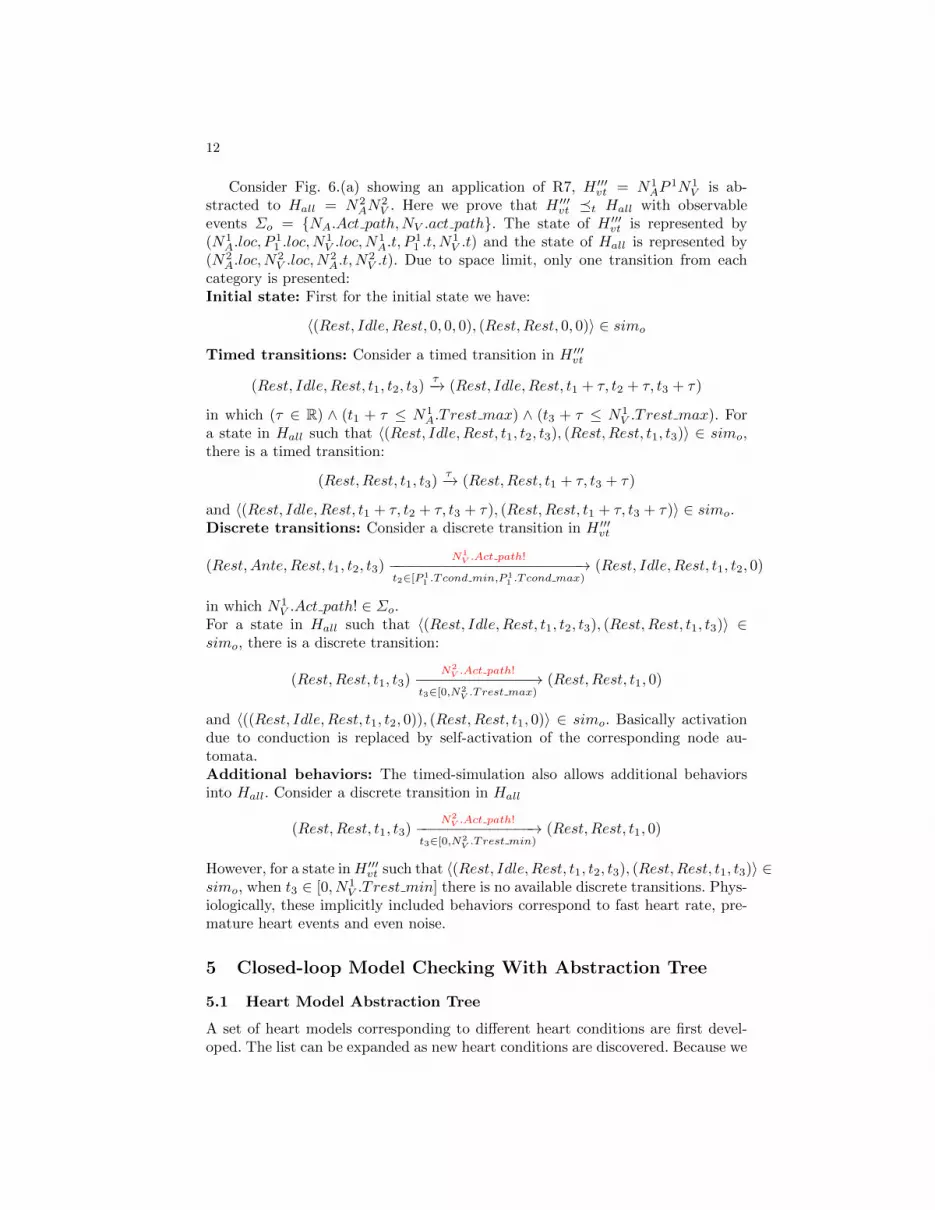
Consider Fig. 6.(a) showing an application of R7, H ′′′vt = N1AP

1N1V is ab-

stracted to Hall = N2AN

2V . Here we prove that H ′′′vt t Hall with observable

events Σo = NA.Act path,NV .act path. The state of H ′′′vt is represented by(N1

A.loc, P11 .loc,N

1V .loc,N

1A.t, P

11 .t, N

1V .t) and the state of Hall is represented by

(N2A.loc,N

2V .loc,N

2A.t, N

2V .t). Due to space limit, only one transition from each

category is presented:Initial state: First for the initial state we have:

〈(Rest, Idle, Rest, 0, 0, 0), (Rest,Rest, 0, 0)〉 ∈ simo

Timed transitions: Consider a timed transition in H ′′′vt

(Rest, Idle, Rest, t1, t2, t3)τ−→ (Rest, Idle, Rest, t1 + τ, t2 + τ, t3 + τ)

in which (τ ∈ R) ∧ (t1 + τ ≤ N1A.T rest max) ∧ (t3 + τ ≤ N1

V .T rest max). Fora state in Hall such that 〈(Rest, Idle,Rest, t1, t2, t3), (Rest,Rest, t1, t3)〉 ∈ simo,there is a timed transition:

(Rest,Rest, t1, t3)τ−→ (Rest,Rest, t1 + τ, t3 + τ)

and 〈(Rest, Idle,Rest, t1 + τ, t2 + τ, t3 + τ), (Rest,Rest, t1 + τ, t3 + τ)〉 ∈ simo.Discrete transitions: Consider a discrete transition in H ′′′vt

(Rest,Ante,Rest, t1, t2, t3)N1

V .Act path!−−−−−−−−−−−−−−−−−−−−−−−→t2∈[P 1

1 .T cond min,P11 .T cond max)

(Rest, Idle, Rest, t1, t2, 0)

in which N1V .Act path! ∈ Σo.

For a state in Hall such that 〈(Rest, Idle, Rest, t1, t2, t3), (Rest,Rest, t1, t3)〉 ∈simo, there is a discrete transition:

(Rest,Rest, t1, t3)N2

V .Act path!−−−−−−−−−−−−−−→t3∈[0,N2

V .Trest max)(Rest,Rest, t1, 0)

and 〈((Rest, Idle,Rest, t1, t2, 0)), (Rest,Rest, t1, 0)〉 ∈ simo. Basically activationdue to conduction is replaced by self-activation of the corresponding node au-tomata.Additional behaviors: The timed-simulation also allows additional behaviorsinto Hall. Consider a discrete transition in Hall

(Rest,Rest, t1, t3)N2

V .Act path!−−−−−−−−−−−−−−→t3∈[0,N2

V .Trest min)(Rest,Rest, t1, 0)

However, for a state inH ′′′vt such that 〈(Rest, Idle, Rest, t1, t2, t3), (Rest,Rest, t1, t3)〉 ∈simo, when t3 ∈ [0, N1

V .T rest min] there is no available discrete transitions. Phys-iologically, these implicitly included behaviors correspond to fast heart rate, pre-mature heart events and even noise.

5 Closed-loop Model Checking With Abstraction Tree

5.1 Heart Model Abstraction Tree

A set of heart models corresponding to different heart conditions are first devel-oped. The list can be expanded as new heart conditions are discovered. Because we

13

NormalSinus

Rhythm

Bradycardia

AV Block

BundleBranchBlock

SinusTachycardia

AtrialFlutter

AVNRT

AtrialFibrillation

PrematureVentricle

Contraction

VentricleTachycardia

VentricleFibrillation R4

R3

R2

R2

R4

R2

R2

R1

R1

R1

R1

R1

R5

R5

R3

R3

R6

R6

R6

R7

R7

R7

R2

R2

R2

R4

R4

R4

𝐻𝑎𝑙𝑙

𝐻𝑛′′

𝐻𝑎𝑡′′′′R2

R2

R4

R4

R4

R2

R4𝐻𝑣𝑡′′

R2R4

𝐻𝑛′𝐻𝑛

𝐻𝑛𝑠𝑟′

𝐻𝑏𝑟’

𝐻𝑎𝑣’

𝐻𝑏𝑏𝑏′

𝐻𝑠𝑡

𝐻𝑏𝑏𝑏

𝐻𝑎𝑣

𝐻𝑏𝑟

𝐻𝑛𝑠𝑟

𝐻𝑠𝑡′

𝐻𝑎𝑡′′ 𝐻𝑎𝑡′′′

𝐻𝑎𝑡′𝐻𝑎𝑡

𝐻𝑎𝑓’’

𝐻𝑎𝑣𝑛’’

𝐻𝑎𝑓𝑖𝑏’’

𝐻𝑎𝑓’

𝐻𝑎𝑣𝑛’

𝐻𝑎𝑓𝑖𝑏’

𝐻𝑝𝑣𝑐′𝐻𝑝𝑣𝑐

𝐻𝑣𝑟 ′′𝐻𝑣𝑟 ′𝐻𝑣𝑟

𝐻𝑣𝑓′′𝐻𝑣𝑓′𝐻𝑣𝑓

𝐻𝑣𝑡 𝐻𝑣𝑡’ 𝐻𝑣𝑡′′′

R4

R4

No

rmal

hea

rt s

tru

ctu

reFa

st A

tria

l Rat

eFa

st V

entr

icu

lar

Rat

e

Models with counter-examples

Fig. 7. Heart Model Abstraction Tree

start from a set of initial models, and each one may be abstracted using a numberof abstraction rules, we have a choice of which rules to apply to which models, andthe order in which to apply them. Depending on which rule is applied when, weend up with different abstract models. Thus we end with an abstraction tree THMfor the heart is created, as shown in Fig. 7.

5.2 Model Checking Procedure

After the abstraction tree is built, it can be used for closed-loop model checking bynon-domain experts. The question is which models to select from the abstractiontree to perform model checking, and provide the most concrete counter-examples.These counter-example are provided to the physicians, along with the heart modelsthat generated them, to determine their physiological validity.

Recall the definition of appropriateness from Section 2. In the technical report[11], we show that a sufficient condition for a model M to be appropriate for arequirement ϕ with monitor Mon is V ar(ϕ) ⊂ V ar(M) ∪ V ar(Mon).

14

Proof. To prove that V ar(ϕ) ⊂ V ar(M) is a sufficient condition for appropri-ateness, we introduce some standard terminology. For an integer n ≥ 1, [n] =1, . . . , n. Given a tuple (a1, a2, . . . , an) and a subset H ⊂ [n], the projectionfunction prH() retains the components indexed by H. E.g., pr1,3((a1, a2, a3)) =(a1, a3).

Let V = V1, . . . , Vn be variables with valuation domains D1, . . . , Dn, respec-tively. Let D = D1 × . . . Dn be the state space. Let AP be the set of atomicpropositions on V, i.e. expressions involving the variables in V. We write V ar(p)for the variables that appear in a given proposition p, and V ar(ϕ) = ∪p in ϕV ar(p).We define the map O : AP → 2D which assigns to each atomic proposition p asubset O(p) of states where the proposition holds. Conversely, O−1(s) is the setof atomic propositions that hold for a state s ∈ D.

Given a proposition p, if a variable v1 is not in V ar(p), then pr1(O(p)) =D1. I.e., p places no constraints on the value of variable v1. Given a trace x =s0s1s3 . . . ∈ Dω, we define a run for x to be the sequence pop1p2 . . . of atomicpropositions such that pi ∈ O−1(si). Let ϕ be a formula on AP . If two traces xand y have the same run and x |= ϕ, then y |= ϕ.

All our abstraction rules are projections: i.e., associated to each abstractionfunction h is a set H ⊂ [n] of indices such that to for every s = (a1, a2, . . . , an) ∈ D,h(s) = prH(s). For rule h4, H = [n].

Now let M be a model, h = pr2,...,n(·), and M ′ = h(M). Suppose thatV ar(ϕ) ⊂ V ar(M ′). Let x ∈ B(M ′) such that

x = s0s1s2 . . . |= ϕ

We want to prove that for any y ∈ h−1(x), y |= ϕ. First note that si ∈ D2×. . .×Dn.Let p0p1p2 . . . be the run corresponding to x. By definition of run, si ∈ O(pi) ∩pr2,...,n(D) = pr2,...,n(O(pi)). Since v1 /∈ V ar(M ′), then v1 /∈ V ar(pi) for all pi inϕ. Therefore

O(pi) = D1 × pr2,...,n(O(pi)) ∀i

For any y ∈ h−1(x), y = s0s1s2 . . . where si = (ai, si) ∈ D. Thus si ∈ O(pi), whichmeans that p0p1 . . . is a run of y as well. Therefore, y |= ϕ.

15

Algorithm 1 Algorithm 2

function [HM]=eligible(HM_tree,Req)BM = root of HM_treewhile (BM is not empty)For every model M in BMIf (Var(Req) is a subset of Var(M)+Var(Mon))Remove M from BMsave M in HMelseadd children of M in BMendifendforendwhileReturn HM

Input: system model PM, abstraction tree for environment HM_tree, requirement ReqOutput: Counter examples CE and corresponding model refinements, if any[HM]=eligible(HM_tree,Req);Mc= HM;while (Mc is not empty)For all M in Mc[satisfied,CE]=ModelChecking(M,PM,Req);Remove M from McIf satisfied==0

add the children of M to Mccache CE

elsesave CE from the parent model

endifendforendwhileReturn all saved CEs and their corresponding models

Fig. 8. Algorithms for closed-loop model checking with abstraction tree

1 23

Fig. 9. Basic timers for a dual chamber pacemaker. AS: Atrial Sense, VS: VentricularSense, AP: Atrial Pacing, VP: Ventricular Pacing.

An algorithm is developed to select the most abstract models from the abstrac-tion tree THM that are appropriate for a requirement Req. The detailed imple-mentation of the algorithm can be found in [11].

Upon requirement violation, an abstract counter-example is returned duringclosed-loop model checking. The counter-example may contain context ambigu-ities that should be resolved before sharing with the physician. An abstractiontree contains the information of how different environment conditions are over-approximated by more abstract models. By exploring the abstraction tree, themost concrete yet unambiguous counter-examples can be sent to the physiciansfor analysis. The detailed implementation of the algorithm can be found in [11].

16

6 Case Study: Closed-loop Model Checking of a DualChamber Pacemaker

6.1 Step 1: The Pacemaker Model

A pacemaker diagnoses heart conditions and delivers electrical pacing to the heartaccording to the timing intervals among timing events from the heart and the pace-maker itself. In this section we use a simple dual chamber pacemaker as examplefor closed-loop model checking. The detailed UPPAAL timed automata implemen-tation of the model can be found in [13]. A dual chamber pacemaker has severalbasic timers, which are shown in Fig. 9:Atrial Escape Interval (AEI) defines the maximum interval between the lastventricular event (VS,VP) to an atrial event (AS,AP). If no AS happened beforethe AEI timer expires, atrial pacing (AP) is delivered to the heart (Marker 1 inFig. 9).Atrio-Ventricular Interval (AVI) defines the maximum interval between themost recent atrial event (AS,AP) to an ventricular event (VS,VP). If no VS hap-pened before AVI timer expires, and the time since the most recent ventricularevent (VS,VP) is no less than URI, ventricular pacing (VP) is delivered to theheart (Marker 3 in Fig. 9).Post-Ventricular Atrial Refractory Period (PVARP) and VentricularRefractory Period (VRP) define the minimum period that a AS or VS canhappen since the most recent ventricular event (VS,VP).

6.2 Step 2: Requirement Encoding

The requirement below is designed to prevent the pacemaker from pacing too fast.If the intervals between self-activations of the atria are between 300ms to 1000ms(60bpm-200bpm), the intervals between ventricular paces should be no shorter than500ms.Self-activations of the atria is mapped to the location of node automaton NAand clock variable NA.t. The requirement can be formalized using the monitorMsing(V P, 500,∞):

Req1 : NA.loc = Rest&&NA.t ∈ [300, 1000]⇒ ¬Msing.loc == Err

6.3 Step 3: Choosing Appropriate Heart Models For the Requirement

To verify the closed-loop system with pacemaker model PM and heart modelabstraction tree THM (Fig. 7) against requirement Req1, the most abstract ap-propriate models are selected from the abstraction tree. The single event mon-itor Msing from Fig. 5.a with variables V ar(Msing) = Msing.t,Msing.loc isused for this requirement. The variables in the requirement are: V ar(Req1) =NA.t, NA.loc,Msing.loc.

At the root level heart model Hall, we have NA.t, NA.loc 6⊂ V ar(Hall) ∪V ar(Msing). As the result, Hall is not appropriate for Req1. All the childrenof Hall: H

′′n , H

′′′′at , H

′′′vt are appropriate for Req1, thus these 3 heart models are

outputted as the most abstract models that are appropriate for Req1.

17

𝐻𝑎𝑙𝑙

𝐻𝑛′′

𝐻𝑎𝑡′′′′

𝐻𝑣𝑡′′

𝐻𝑛′𝐻𝑛

𝐻𝑎𝑡′′ 𝐻𝑎𝑡′′′

𝐻𝑎𝑡′𝐻𝑎𝑡

𝐻𝑣𝑡 𝐻𝑣𝑡’ 𝐻𝑣𝑡′′′

𝐻𝑎𝑣𝑛’’

𝐻𝑎𝑓𝑖𝑏’’

𝐻𝑎𝑣𝑛’

𝐻𝑎𝑓𝑖𝑏’

𝐻𝑝𝑣𝑐′𝐻𝑝𝑣𝑐

𝐻𝑎𝑓’’𝐻𝑎𝑓’

𝐻𝑎𝑣𝑛

𝐻𝑎𝑓𝑖𝑏

𝐻𝑎𝑓

A

V

IAVIA

V

IAVIA

V

IAVI

VP VP VP

<500

𝐂𝐄𝒏

PVC A

V

IAVIA

V

IAVI A

V

IAVI

<500

VP VP VP

cond cond cond

𝐂𝐄𝑷𝑽𝑪

A

V

IAVIA

V

IAVI A

V

IAVI

VP VP VP

<500

𝐂𝐄𝐚𝐟

Heart

Pacemaker

Heart

Pacemaker

Heart

Pacemaker

Fig. 10. Finding the most concrete counter-examples using the abstraction tree

6.4 Step 4: Return The Most Concrete Counter-Examples

After the appropriate models for Req1 are selected, we have the initial set HM =H ′′n , H ′′′′at , H ′′′vt. Then we run Algorithm 2. By model checking on all 3 initialmodels in UPPAAL we have:

H ′′n ||PM 6|= Req1;H ′′′′at ||PM 6|= Req1;H ′′′vt ||PM 6|= Req1

The abstraction tree is then further explored. The heart models with counter-examples are illustrated in Fig. 7, and the most refined heart models with counter-examples are: Hn;Hpvc;Haf ;Havn;Hafib.

6.5 Step 5: Analysis of the Counter-examples

The counter-examples are then shared with physicians for analysis. In Fig. 10 wedemonstrate 3 counter-examples. In the counter-examples, the first signal showsthe intrinsic heart signals over time with up arrows as atrial activations and downarrows as ventricular activations. The second signal shows the pacemaker outputswith up arrows as atrial pacing and down arrows as ventricular pacing.

CEn is returned by Hn and none of its children models violate the require-ment. By careful analysis we found that CEn features the combination of fastintrinsic atrial rate and prolonged A-V conduction delay, which is the combina-tion of heart conditions Hst and Hav. This scenario shows that the abstractionrules can introduce physiological heart conditions that were not explicitly modeledin the initial model set. The pacemaker improved the open-loop heart conditionby pacing the ventricles AV I after each atrial event, which is a correct operationof the pacemaker despite the requirement violation.

CEpvc has a very similar execution to CEn. However, the activations of theatrial node are triggered by retrograde conduction from ventricular paces (markercond). The atrial activations trigger another ventricular pace after AV I, which willtrigger another retrograde conduction. In this case the heart rate is inappropriately

18

high, which corresponds to a dangerous closed-loop behavior referred to as EndlessLoop Tachycardia.

In CEaf the atrial rate is very high, which is also a sub-optimal but not dan-gerous heart condition. However, the ventricular rate can stay normal due to theblocking property of the AV node. Despite the filters in the pacemaker, the pace-maker still paces the ventricle for every 3 atrial activations, which extends fastatrial rate to more dangerous fast ventricular rate. This scenario is referred to asAtrial Tachycardia Response of a pacemaker.

From the analysis, pacemaker operations in CEpvc and CEaf must be re-vised. However, the revision should not affect the behavior in CEn. This exampledemonstrates that counter-examples from more refined models provide more de-tailed mechanism of the requirement violations, and distinguish the physiologicalconditions that can trigger the violations. The information is helpful for debuggingand improving the algorithm. The physicians can also improve the physiologicalrequirement so that these heart conditions can be then considered case by case.

7 Conclusions and Future ResearchIn this paper we addressed the challenges for environment modeling during closed-loop model checking of medical device software. Physiological abstraction rules canbe defined to increase coverage of physiological conditions beyond explicitly mod-eled conditions. By using the abstraction tree constructed by applying the phys-iological abstraction rules, closed-loop model checking returns the most concretecounter-examples with physiological context to the physician when a physiologicalrequirement is violated. In this paper we use implantable pacemaker as case studybut the framework can extend to other domains.

In the future, application of the abstraction rules will be automated. The ap-plication of this framework can also be extended to other domains like automotive.

References

[1] Matlab R2013a Documentation → Stateflow. http://www.mathworks.com/help/toolbox/stateflow.

[2] Personal communication with Paul L. Jones, Senior Systems/Software Engi-neer, Office of Science and Engineering Laboratories, Center for Devices andRadiological Health, US FDA. August, 2010.

[3] R. Alur, C. Courcoubetis, and D. Dill. Model-checking for real-time systems.In Logic in Computer Science, 1990. LICS ’90, Proceedings., Fifth AnnualIEEE Symposium on e, pages 414–425, 1990.

[4] R. Alur and D. L. Dill. A Theory of Timed Automata. Theoretical ComputerScience, 126:183–235, 1994.

[5] T. Chen, M. Diciolla, M. Kwiatkowska, and A. Mereacre. Quantitative veri-fication of implantable cardiac pacemakers over hybrid heart models. Infor-mation and Computation, 236(0):87 – 101, 2014.

[6] E. Clarke, O. Grumberg, S. Jha, Y. Lu, and H. Veith. Counter Example-Guided Abstraction Refinement for Symbolic Model Checking. J. ACM,50(5):752–794, 2003.

[7] Dominique Mery and Neeraj Kumar Singh. Pacemaker’s Functional Behaviorsin Event-B. Research Report, 2009.

19

[8] U. FDA. Medical Device Recall Report FY2003 to FY2012. 2012.[9] U. FDA. Human Subject Protection; Acceptance of Data from Clinical Stud-

ies for Medical Devices; Proposed Rule. 2013.[10] M. A. Islam, A. Murthy, A. Girard, S. A. Smolka, and R. Grosu. Composition-

ality results for cardiac cell dynamics. In Proceedings of the 17th InternationalConference on Hybrid Systems, HSCC ’14, pages 243–252, 2014.

[11] Z. Jiang, H. Abbas, P. Mosterman, and R. Mangharam. Tech Report:Abstraction-Tree For Closed-loop Model Checking of Medical Devices.http://repository.upenn.edu/mlab papers/73, 2015.

[12] Z. Jiang, A. Connolly, and R. Mangharam. Using the Virtual Heart Modelto Validate the Mode-Switch Pacemaker Operation. IEEE Engineering inMedicine and Biology Society, pages 6690 –6693, 2010.

[13] Z. Jiang, M. Pajic, R. Alur, and R. Mangharam. Closed-loop verification ofmedical devices with model abstraction and refinement. International Journalon Software Tools for Technology Transfer, pages 1–23, 2013.

[14] Z. Jiang, M. Pajic, A. Connolly, S. Dixit, and R. Mangharam. Real-TimeHeart Model for Implantable Cardiac Device Validation and Verification. In22nd Euromicro Conference on Real-Time Systems (ECRTS), pages 239 –248,July 2010.

[15] Z. Jiang, M. Pajic, and R. Mangharam. Cyber-Physical Modeling of Im-plantable Cardiac Medical Devices. Proceeding of IEEE Special Issue onCyber-Physical Systems, 2011.

[16] Z. Jiang, M. Pajic, and R. Mangharam. Model-based Closed-loop Testingof Implantable Pacemakers. In ICCPS’11: ACM/IEEE 2nd Intl. Conf. onCyber-Physical Systems, 2011.

[17] M. Josephson. Clinical Cardiac Electrophysiology. Lippincot Williams andWilkins, 2008.

[18] K. Larsen, P. Pettersson, and W. Yi. Uppaal in a Nutshell. InternationalJournal on Software Tools for Technology Transfer (STTT), 1997.

[19] K. Sandler, L. Ohrstrom, L. Moy, and R. McVay. Killed by Code: SoftwareTransparency in Implantable Medical Devices. Software Freedom Law Center,2010.

[20] N. A. Trayanova and P. M. Boyle. Advances in modeling ventricular arrhyth-mias: from mechanisms to the clinic. Wiley Interdisciplinary Reviews: SystemsBiology and Medicine, 6(2):209–224, 2014.