Lazy Abstraction for Size-Change Termination?

Michael Codish1, Carsten Fuhs2, Jurgen Giesl2, and Peter Schneider-Kamp3

1 Department of Computer Science, Ben-Gurion University, Israel2 LuFG Informatik 2, RWTH Aachen University, Germany

3 IMADA, University of Southern Denmark, Odense, Denmark

Abstract. Size-change termination is a widely used means of provingtermination where source programs are first abstracted to size-changegraphs which are then analyzed to determine if they satisfy the size-change termination property. Here, the choice of the abstraction is crucialto the success of the method, and it is an open problem how to choosean abstraction such that no critical loss of precision occurs. This papershows how to couple the search for a suitable abstraction and the test forsize-change termination via an encoding to a single SAT instance. In thisway, the problem of choosing the right abstraction is solved en passantby a SAT solver. We show that for the setting of term rewriting, theintegration of this approach into the dependency pair framework workssmoothly and gives rise to a new class of size-change reduction pairs.We implemented size-change reduction pairs in the termination proverAProVE and evaluated their usefulness in extensive experiments.

1 Introduction

Proving termination is a fundamental problem in verification. The challenge oftermination analysis is to design a program abstraction that captures the proper-ties needed to prove termination as often as possible, while providing a decidablesufficient criterion for termination. The size-change termination method (SCT)[21] is one such technique where programs are abstracted to size-change graphs.They describe how the sizes of program data are affected by the transitionsmade in a computation. Size is measured by a well-founded base order. A set ofsize-change graphs has the SCT property iff for every path through any infiniteconcatenation of these graphs, a value would descend infinitely often w.r.t. thebase order. The well-foundedness of the base order then leads to a contradiction,which implies termination of the original program. Lee et al. prove in [21] thatthe problem to determine if a set of size-change graphs has the SCT property isPSPACE-complete. The size-change termination method has been successfullyapplied in a variety of different application areas [2, 7, 19, 25, 28, 29].

Another approach emerges from the term rewriting community where termi-nation proofs are performed by identifying suitable orders on terms and showingthat every transition in a computation leads to a reduction w.r.t. the order. This? Supported by the G.I.F. grant 966-116.6, the DFG grant GI 274/5-3, and the Danish

Natural Science Research Council.

approach provides a decidable sufficient termination criterion for a given class oforders and can be considered as a program abstraction because terms are viewedmodulo the order. Tools based on these techniques have been successfully appliedto prove termination automatically for a wide range of different programminglanguages (e.g., Prolog [23, 27], Haskell [17], and Java Bytecode [24]).

A major bottleneck when applying SCT is due to the fact that this is a 2-phase process: First, a suitable program abstraction must be found, and then, theresulting size-change graphs are checked for termination. It is an open problemhow to choose an abstraction such that no critical loss of precision occurs. Thus,our aim is to couple the search for a suitable abstraction with the test for size-change termination. To this end we model the search for an abstraction as thesearch for an order on terms (like in term rewriting). Then we can encode boththe abstraction and the test for the SCT property into a single SAT instance.

Using a SAT-based search for orders to prove termination is well establishedby now. For instance [8, 9, 13, 26, 30] describe encodings for RPO, polynomial or-ders, or KBO. However, there is one major obstacle when using SAT for SCT.SCT is PSPACE-complete and hence (unless NP = PSPACE), there is no polyno-mial-size encoding of SCT to SAT. Thus, we focus on a subset of SCT which is inNP and can therefore be effectively encoded to SAT. This subset, called SCNP,is introduced by Ben-Amram and Codish in [5] where experimental evidenceindicates that the restriction to this subset of SCT hardly makes any differencein practice. We illustrate our approach in the context of term rewrite systems(TRSs). The basic idea is to give a SAT encoding for the following question:

For a given TRS (and a class of base orders such as RPO), is there a baseorder such that the resulting size-change graphs have the SCT property?

In [29], Thiemann and Giesl also apply the SCT method to TRSs and show howto couple it with the dependency pair (DP) method [1]. However, they take the2-phase approach, first (manually) choosing a base order, and then checking ifthe induced size-change graphs satisfy the SCT property. Otherwise, one mighttry a different order. The implementation of [29] in the tool AProVE [15] onlyuses the (weak) embedding order in combination with argument filters [1] as baseorder. It performs a naive search which enumerates all argument filters. The newapproach in this paper leads to a significantly more powerful implementation.

Using SCNP instead of SCT has an additional benefit. SCNP can be directlysimulated by a new class of orders which can be used for reduction pairs in theDP framework. Thus, the techniques (or “processors”) of the DP framework donot have to be modified at all for the combination with SCNP. This makes theintegration of the size-change method with DPs much smoother than in [29] andit also allows to use this integration directly in arbitrary (future) extensions ofthe DP framework. The orders simulating SCNP are novel in the rewriting area.

The paper is structured as follows: Sect. 2 and 3 briefly present the DPframework and the SCT method for DPs. Sect. 4 adapts the SCNP approach toterm rewriting. Sect. 5 shows how to encode the search for a base order whichsatisfies the SCNP property into a single SAT problem. Sect. 6 presents ourexperimental evaluation in the AProVE tool [15]. We conclude in Sect. 7.

2 Term Rewrite Systems and Dependency Pairs

We assume familiarity with term rewriting [3] and briefly introduce the mainideas of the DP method. The basic idea is (i) to describe all (finitely many)paths in the program from one function call to the next by special rewrite rules,called dependency pairs. Then (ii) one has to prove that these paths cannotfollow each other infinitely often in a computation.

To represent a path from a function call of f with arguments s1, . . . , sn to afunction call of g with arguments t1, . . . , tm, we extend the signature by two newtuple symbols F and G. Then a function call is represented by a tuple term, i.e.,by a term rooted by a tuple symbol, but where no tuple symbols occur belowthe root. The DP for this path is the rule F (s1, . . . , sn)→ G(t1, . . . , tm).

The DP framework operates on DP problems (P,R), which are pairs of twoTRSs. Here, for all s → t ∈ P, both s and t are tuple terms, whereas for alll→ r ∈ R, both l and r are base terms, i.e., they do not contain tuple symbols. Inthe initial DP problem (P,R), P contains all DPs and R contains all rules of theTRS. Then, to show that this problem does not allow infinite chains of functioncalls, there is a large number of processors for analyzing and simplifying suchDP problems. We refer to [1, 14, 16, 18] for further details on the DP framework.

The most common processor for simplifying DP problems is the reductionpair processor. In a reduction pair (%,�), % is a stable monotonic4 quasi-ordercomparing either two tuple terms or two base terms. Moreover, � is a stablewell-founded order on terms, where % and � are compatible (i.e., � ◦ % ⊆ �and % ◦ � ⊆ �). Given such a reduction pair and a DP problem (P,R), if wecan show a weak decrease (i.e., a decrease w.r.t. %) for all rules from R and allDPs from P, we can delete all those DPs from P that are strictly decreasing (i.e.,that decrease w.r.t. �). In other words, we are asking the following question:

For a given DP problem (P,R), is there a reduction pair that orients allrules of R and P weakly and at least one of the rules of P strictly?

If we can delete all DPs by repeatedly applying this processor, then the initialDP problem does not allow infinite chains of function calls. Consequently, thereis no infinite reduction with the original TRS R, i.e., R is terminating.

3 Size-Change Termination and Dependency Pairs

Size-change termination [21] is a program abstraction where termination is de-cidable. As mentioned in the introduction, an abstract program is a finite set ofsize-change graphs which describe, in terms of size-change, the possible transi-tions between consecutive function calls in the original program.

Size-change termination and the DP framework have some similarities: (i)size-change graphs provide a representation of the paths from one function callto the next, and (ii) in a second stage we show that these graphs do not allowinfinite descent. So these steps correspond to steps (i) and (ii) in the DP method.

The main difference between SCT and the DP method is the stage when the4 If monotonicity of % is not required, we speak of a non-monotonic reduction pair.

(a) F1//

��99

99 F1

F2 F2

F1

��99

99 F1

F2

BB�������F2

(b) F1//

��9999999 F1

F2 F2

F1 F1

F2//

BB�������F2

F1// F1

F2// F2

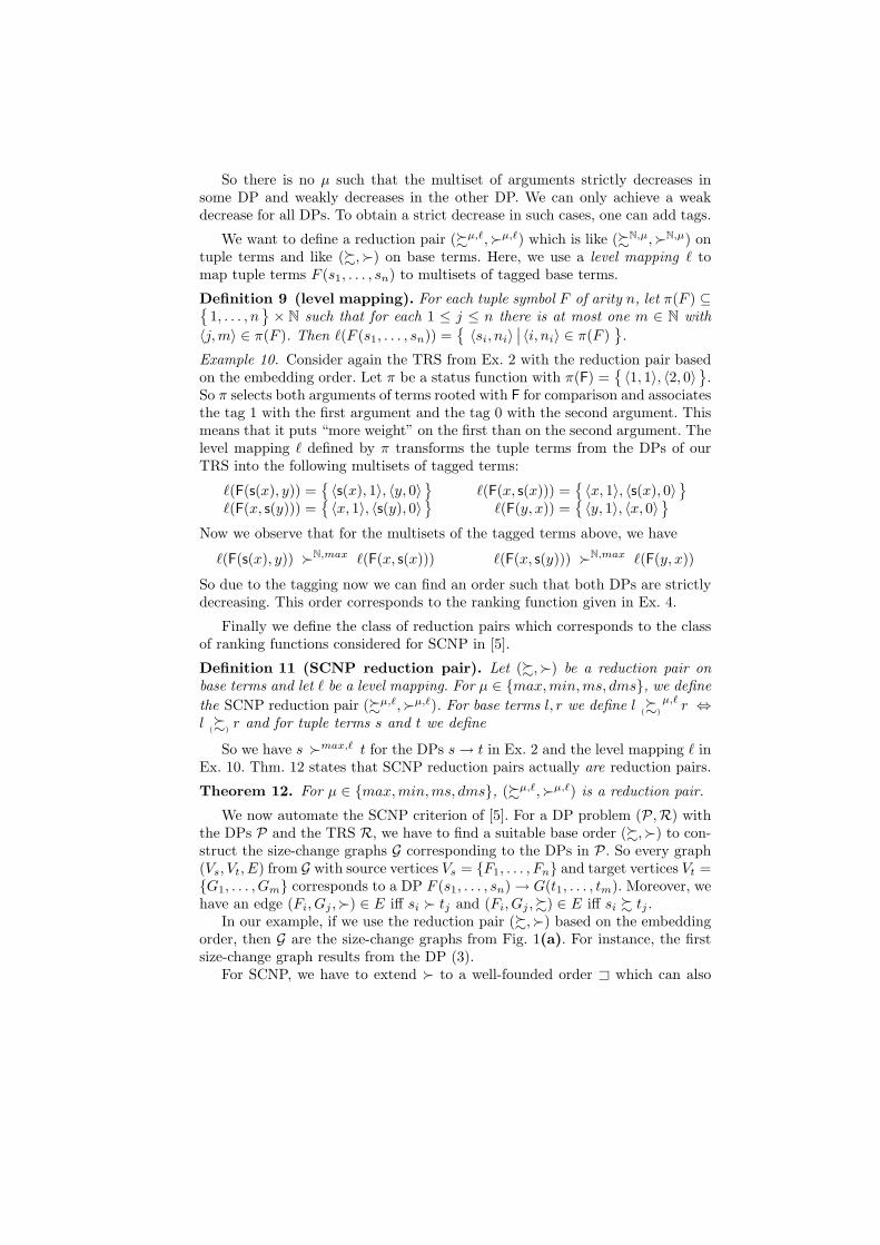
Fig. 1. Size-change graphs from Ex. 2

undecidable termination problem is abstracted to a decidable one. For SCT, weuse a base order to obtain the finite representation of the paths by size-changegraphs. For DPs, no such abstraction is performed and, indeed, the terminationof a DP problem is undecidable. Here, the abstraction step is only the secondstage where typically a decidable class of base orders is used.

The SCT method can be used with any base order. It only requires the infor-mation which arguments of a function call become (strictly or weakly) smallerw.r.t. the base order. To prove termination, the base order has to be well founded.For the adaptation to TRSs we will use a reduction pair (%,�) for this purposeand introduce the notion of a size-change graph directly for dependency pairs.

If the TRS has a DP F (s1, . . . , sn)→ G(t1, . . . , tm), then the correspondingsize-change graph has nodes {F1, . . . , Fn, G1, . . . , Gm} representing the argumentpositions of F andG. The labeled edges in the size-change graph indicate whetherthere is a strict or weak decrease between these arguments.

Definition 1 (size-change graphs). Let (%,�) be a (possibly non-monotonic)reduction pair on base terms, and let F (s1, . . . , sn)→ G(t1, . . . , tm) be a DP. Thesize-change graph resulting from this DP and this reduction pair is the graph(Vs, Vt, E) with source vertices Vs = {F1, . . . , Fn}, target vertices Vt = {G1, . . . ,Gm}, and labeled edges E = {(Fi, Gj ,�) | si � tj} ∪ {(Fi, Gj ,%) | si % tj}.

Size-change graphs are depicted as in Fig. 1. Each graph consists of sourcevertices, on the left, target vertices, on the right, and edges drawn as full anddashed arrows to indicate strict and weak decrease (i.e., corresponding to “�”and “%”, respectively). We introduce the main ideas underlying SCT by example.

Example 2. Consider the TRS {(1), (2)}. It has the DPs (3) and (4).

f(s(x), y)→ f(x, s(x)) (1)f(x, s(y))→ f(y, x) (2)

F(s(x), y)→ F(x, s(x)) (3)F(x, s(y))→ F(y, x) (4)

We use a reduction pair based on the embedding order where s(x) � x, s(y) � y,s(x) % s(x), s(y) % s(y). Then we get the size-change graphs in Fig. 1(a). Be-tween consecutive function calls, the first argument decreases in size or becomessmaller than the original second argument. In both cases, the second argumentweakly decreases compared to the original first argument. By repeated compo-sition of the size-change graphs, we obtain the three “idempotent” graphs inFig. 1(b). All of them exhibit in situ decrease (at F1 in the first graph, at F2 inthe second graph, and at both F1 and F2 in the third graph). This means thatthe original size-change graphs from Fig. 1(a) satisfy the SCT property.

Earlier work [29] shows how to combine SCT with term rewriting. Let R bea TRS and (%,�) a reduction pair such that if s � t (or s % t) then t containsno defined symbols of R, i.e., no root symbols of left-hand sides of rules fromR.5 Let G be the set of size-change graphs resulting from all DPs with (%,�). In[29] the authors prove that if G satisfies SCT then R is innermost terminating.

Example 3. If one restricts the reduction pair in Ex. 2 to just terms withoutdefined symbols, then one still obtains the same size-change graphs. Since thesegraphs satisfy the SCT property, one can conclude that the TRS is indeed in-nermost terminating. Note that to show termination without SCT, an order likeRPO would fail (since the first rule requires a lexicographic comparison andthe second requires a multiset comparison). While termination could be provedby polynomial orders, as in [29] one could unite these rules with the rules forthe Ackermann function. Then SCT with the embedding order would still work,whereas a direct application of RPO or polynomial orders fails.

So our example illustrates a major strength of SCT. A proof of termination isobtained by using just a simple base order and by considering each idempotentgraph in the closure under composition afterwards. In contrast, without SCT,one would need more complex termination arguments.

In [29] the authors show that when constructing the size-change graphs fromthe DPs, one can even use arbitrary reduction pairs as base orders, providedthat all rules of the TRS are weakly decreasing. In other words, this previouswork essentially addresses the following question for any DP problem (P,R):

For a given base order where R is weakly decreasing, do all idempotentsize-change graphs, under composition closure, exhibit in situ decrease?

Note that in [29], the base order is always given and the only way to search fora base order automatically would be a hopeless generate-and-test approach.

4 Approximating SCT in NP

In [5] the authors identify a subset of SCT, called SCNP, that is powerful enoughfor practical use and is in NP. For SCNP just as for SCT, programs are abstractedto sets of size-change graphs. But instead of checking SCT by the closure undercomposition, one identifies a suitable ranking function to certify the terminationof programs described by the set of graphs. Ranking functions map “programstates” to elements of a well-founded domain and one has to show that they(strictly) decrease on all program transitions described by the size-change graphs.

In the rewriting context, program states are terms. Here, instead of a rankingfunction one can use an arbitrary stable well-founded order A. Let (Vs, Vt, E) bea size-change graph with source vertices Vs = {F1, . . . , Fn}, target vertices Vt ={G1, . . . , Gm}, and let (%,�) be the reduction pair on base terms which wasused for the construction of the graph. Now the goal is to extend the order � toa well-founded order A which can also compare tuple terms and which satisfies5 Strictly speaking, this is not a reduction pair, since it is only stable under substitu-

tions which do not introduce defined symbols.

the size-change graph (i.e., F (s1, . . . , sn) A G(t1, . . . , tm)). Similarly, we say thatA satisfies a set of size-change graphs iff it satisfies all the graphs in the set.

If the size-change graphs describe the transitions of a program, then theexistence of a corresponding ranking function obviously implies termination ofthe program. As in [29], to ensure that the size-change graphs really describethe transitions of the TRS correctly, one has to impose suitable restrictions onthe reduction pair (e.g., by demanding that all rules of the TRS are weaklydecreasing w.r.t. %). Then one can indeed conclude termination of the TRS.

In [22], a class of ranking functions is identified which can simulate SCT.So if a set of size-change graphs has the SCT property, then there is a rankingfunction of that class satisfying these size-change graphs. However, this class istypically exponential in size [22]. To obtain a subset of SCT in NP, [5] considersa restricted class of ranking functions. A set of size-change graphs has the SCNPproperty iff it is satisfied by a ranking function from this restricted class.

Our goal is to adapt this class of ranking functions to term rewriting. Themain motivation is to facilitate the simultaneous search for a ranking functionon the size-change graphs and for the base order which is used to derive the size-change graphs from a TRS. It means that we are searching both for a programabstraction to size-change graphs, and also for the ranking function which provesthat these graphs have the SCNP (and hence also the SCT) property.

This is different from [5], where the concrete structure of the program has al-ready been abstracted away to size-change graphs that must be given as inputs. Itis also different from the earlier adaption of SCT to term rewriting in [29], wherethe base order was fixed. As shown by the experiments with [29] in Sect. 6, fixingthe base order for the size-change graphs leads to severe limitations in power.

The following example illustrates the SCNP property and presents a rankingfunction (resp. a well-founded order A) satisfying a set of size-change graphs.

Example 4. Consider the TRS from Ex. 2 and its size-change graphs in Fig. 1(a).Here, the base order is the reduction pair (%,�) resulting from the embeddingorder. We now extend � to an order A which can also compare tuple terms andwhich satisfies the size-change graphs in this example. To compare tuple termsF(s1, s2) and F(t1, t2), we first map them to the multisets { 〈s1, 1〉, 〈s2, 0〉 } and{ 〈t1, 1〉, 〈t2, 0〉 } of tagged terms (where a tagged term is a pair of a term and anumber). Now a multiset S of tagged terms is greater than a multiset T iff forevery 〈t,m〉 ∈ T there is an 〈s, n〉 ∈ S where s � t or both s % t and n > m.

For the first graph, we have s1 � t1 and s1 % t2 and hence the multiset{ 〈s1, 1〉, 〈s2, 0〉 } is greater than { 〈t1, 1〉, 〈t2, 0〉 }. For the second graph, s1 % t2and s2 � t1 also implies that the multiset { 〈s1, 1〉, 〈s2, 0〉 } is greater than{ 〈t1, 1〉, 〈t2, 0〉 }. Thus, if we define our well-founded order A in this way, thenit indeed satisfies both size-change graphs of the example. Since this order Abelongs to the class of ranking functions defined in [5], this shows that the size-change graphs in Fig. 1(a) have the SCNP property.

In term rewriting, size-change graphs correspond to DPs and the arcs of thesize-change graphs are built by only comparing the arguments of the DPs (whichare base terms). The ranking function then corresponds to a well-founded order

on tuple terms. We now reformulate the class of ranking functions of [5] in theterm rewriting context by defining SCNP reduction pairs. The advantage of thisreformulation is that it allows us to integrate the SCNP approach directly intothe DP framework and that it allows a SAT encoding of both the search forsuitable base orders and of the test for the SCNP property. In [5], the class ofranking functions for SCNP is defined incrementally. We follow this, but adaptthe definitions of [5] to the term rewriting setting and prove that the resultingorders always constitute reduction pairs. More precisely, we proceed as follows:step one: (%,�) is an arbitrary reduction pair on base terms that we start with(e.g., based on RPO and argument filters or on polynomial orders). The mainobservation that can be drawn from the SCNP approach is that it is helpfulto compare base terms and tuple terms in a different way. Thus, our goal is toextend (%,�) appropriately to a reduction pair (w,A) that can also comparetuple terms. By defining (w,A) in the same way as the ranking functions of [5],it can simulate the SCNP approach.step two: (%N,�N) is a reduction pair on tagged base terms, i.e., on pairs〈t, n〉, where t is a base term and n ∈ N. Essentially, (%N,�N) is a lexicographiccombination of the reduction pair (%,�) with the usual order on N.step three: (%N,µ,�N,µ) extends (%N,�N) to compare multisets of tagged baseterms. The status µ determines how (%N,�N) is extended to multisets.step four: (%µ,`,�µ,`) is a full reduction pair (i.e., it is the reduction pair(w,A) we were looking for). The level mapping ` determines which argumentsof a tuple term are selected and tagged, resulting in a multiset of tagged baseterms. On tuple terms, (%µ,`,�µ,`) behaves according to (%N,µ,�N,µ) on themultisets as determined by `, and on base terms, it behaves like (%,�).

Thus, we start with extending a reduction pair (%,�) on base terms to areduction pair (%N,�N) on tagged base terms. We compare tagged terms lexi-cographically by (%,�) and by the standard orders ≥ and > on numbers.

Definition 5 (comparing tagged terms). Let (%,�) be a reduction pair onterms. We define the corresponding reduction pair (%N,�N) on tagged terms:

– 〈t1, n1〉 %N 〈t2, n2〉 ⇔ t1 � t2 ∨ (t1 % t2 ∧ n1 ≥ n2).

– 〈t1, n1〉 �N 〈t2, n2〉 ⇔ t1 � t2 ∨ (t1 % t2 ∧ n1 > n2).

The motivation for tagged terms is that we will use different tags (i.e., num-bers) for the different argument positions of a function symbol. For instance,when comparing the terms s = F(s(x), y) and t = F(x, s(x)) as in Ex. 4, onecan assign the tags 1 and 0 to the first and second argument position of F, re-spectively. Then, if (%,�) is the reduction pair based on the embedding order,we have 〈s(x), 1〉 �N 〈x, 1〉 and 〈s(x), 1〉 �N 〈s(x), 0〉. In other words, the firstargument of s is greater than both the first and the second argument of t.

The following lemma states that if (%,�) is a reduction pair on terms, then(%N,�N) is a reduction pair on tagged terms (where we do not require mono-tonicity, since monotonicity is not defined for tagged terms). This lemma will beneeded for our main theorem (Thm. 12) which proves that the reduction pairdefined to simulate SCNP is really a reduction pair.

Lemma 6 (reduction pairs on tagged terms). Let (%,�) be a reductionpair. Then (%N,�N) is a non-monotonic reduction pair on tagged terms.6

The next step is to introduce a “reduction pair” (%N,µ,�N,µ) on multisetsof tagged base terms, where µ is a status which determines how (%N,�N) is ex-tended to multisets. Of course, there are many possibilities for such an extension.In Def. 7, we present the four extensions which correspond to the ranking func-tions defining SCNP in [5]. The main difference to the definitions in [5] is thatwe do not restrict ourselves to total base orders. Hence, the notions of maximumand minimum of a multiset of terms are not defined in the same way as in [5].

Definition 7 (multiset extensions of reduction pairs). Let (%,�) be areduction pair on (tagged) terms. We define an extended reduction pair (%µ,�µ)on multisets of (tagged) terms, for µ ∈ {max,min,ms, dms}. Let S and T bemultisets of (tagged) terms.

1. (max order) S %max T holds iff ∀t∈T. ∃s∈S. s % t.S �max T holds iff S 6= ∅ and ∀t∈T. ∃s∈S. s � t.

2. (min order) S %min T holds iff ∀s∈S. ∃t∈T. s % t.S �min T holds iff T 6= ∅ and ∀s∈S. ∃t∈T. s � t.

3. (multiset order [10]) S �ms T holds iff S = Sstrict ]{s1, . . . , sk

}, T =

Tstrict ]{t1, . . . , tk

}, Sstrict �max Tstrict, and si % ti for 1 ≤ i ≤ k.

S %ms T holds iff S = Sstrict ]{s1, . . . , sk

}, T = Tstrict ]

{t1, . . . , tk

},

either Sstrict �max Tstrict or Sstrict = Tstrict = ∅, and si % ti for 1 ≤ i ≤ k.4. (dual multiset order [4]) S �dms T holds iff S = Sstrict ]

{s1, . . . , sk

},

T = Tstrict ]{t1, . . . , tk

}, Sstrict �min Tstrict, and si % ti for 1 ≤ i ≤ k.

S %dms T holds iff S = Sstrict ]{s1, . . . , sk

}, T = Tstrict ]

{t1, . . . , tk

},

either Sstrict �min Tstrict or Sstrict = Tstrict = ∅, and si % ti for 1 ≤ i ≤ k.

Here �ms is to the standard multiset extension of an order � as used, e.g.,for the classical definition of RPO. However, our use of tagged terms as elementsof the multiset introduces a lexicographic aspect that is missing in RPO.

Example 8. Consider again the TRS from Ex. 2 with the reduction pair basedon the embedding order. We have {s(x), y} %max {x, s(x)}, since for both termsin {x, s(x)} there is an element in {s(x), y} which is weakly greater (w.r.t. %).Similarly, {x, s(y)} %max {y, x}. However, {x, s(y)} 6�max {y, x}, since not ev-ery element from {y, x} has a strictly greater one in {x, s(y)}. We also have{x, s(y)} %min {y, x}, but {s(x), y} 6%min {x, s(x)}, since for y in {s(x), y}, thereis no term in {x, s(x)} which is weakly smaller.

We have {s(x), y} 6�ms {x, s(x)}, since even if we take {s(x)} �max {x}, westill do not have y % s(x). Moreover, also {s(x), y} 6%ms {x, s(x)}. Otherwise,for every element of {x, s(x)} there would have to be a different weakly greaterelement in {s(x), y}. In contrast, we have {x, s(y)} �ms {y, x}. The element s(y)is replaced by the strictly smaller element y and for the remaining element x onthe right-hand side there is a weakly greater one on the left-hand side. Similarly,we also have {s(x), y} 6%dms {x, s(x)} and{x, s(y)} �dms {y, x}.6 All proofs can be found in [6].

So there is no µ such that the multiset of arguments strictly decreases insome DP and weakly decreases in the other DP. We can only achieve a weakdecrease for all DPs. To obtain a strict decrease in such cases, one can add tags.

We want to define a reduction pair (%µ,`,�µ,`) which is like (%N,µ,�N,µ) ontuple terms and like (%,�) on base terms. Here, we use a level mapping ` tomap tuple terms F (s1, . . . , sn) to multisets of tagged base terms.

Definition 9 (level mapping). For each tuple symbol F of arity n, let π(F ) ⊆{1, . . . , n

}× N such that for each 1 ≤ j ≤ n there is at most one m ∈ N with

〈j,m〉 ∈ π(F ). Then `(F (s1, . . . , sn)) ={〈si, ni〉

∣∣ 〈i, ni〉 ∈ π(F )}

.

Example 10. Consider again the TRS from Ex. 2 with the reduction pair basedon the embedding order. Let π be a status function with π(F) =

{〈1, 1〉, 〈2, 0〉

}.

So π selects both arguments of terms rooted with F for comparison and associatesthe tag 1 with the first argument and the tag 0 with the second argument. Thismeans that it puts “more weight” on the first than on the second argument. Thelevel mapping ` defined by π transforms the tuple terms from the DPs of ourTRS into the following multisets of tagged terms:

`(F(s(x), y)) ={〈s(x), 1〉, 〈y, 0〉

}`(F(x, s(x))) =

{〈x, 1〉, 〈s(x), 0〉

}`(F(x, s(y))) =

{〈x, 1〉, 〈s(y), 0〉

}`(F(y, x)) =

{〈y, 1〉, 〈x, 0〉

}Now we observe that for the multisets of the tagged terms above, we have

`(F(s(x), y)) �N,max `(F(x, s(x))) `(F(x, s(y))) �N,max `(F(y, x))

So due to the tagging now we can find an order such that both DPs are strictlydecreasing. This order corresponds to the ranking function given in Ex. 4.

Finally we define the class of reduction pairs which corresponds to the classof ranking functions considered for SCNP in [5].

Definition 11 (SCNP reduction pair). Let (%,�) be a reduction pair onbase terms and let ` be a level mapping. For µ ∈ {max,min,ms, dms}, we definethe SCNP reduction pair (%µ,`,�µ,`). For base terms l, r we define l (%)

µ,` r ⇔l (%) r and for tuple terms s and t we define

So we have s �max,` t for the DPs s→ t in Ex. 2 and the level mapping ` inEx. 10. Thm. 12 states that SCNP reduction pairs actually are reduction pairs.

Theorem 12. For µ ∈ {max,min,ms, dms}, (%µ,`,�µ,`) is a reduction pair.

We now automate the SCNP criterion of [5]. For a DP problem (P,R) withthe DPs P and the TRS R, we have to find a suitable base order (%,�) to con-struct the size-change graphs G corresponding to the DPs in P. So every graph(Vs, Vt, E) from G with source vertices Vs = {F1, . . . , Fn} and target vertices Vt ={G1, . . . , Gm} corresponds to a DP F (s1, . . . , sn)→ G(t1, . . . , tm). Moreover, wehave an edge (Fi, Gj ,�) ∈ E iff si � tj and (Fi, Gj ,%) ∈ E iff si % tj .

In our example, if we use the reduction pair (%,�) based on the embeddingorder, then G are the size-change graphs from Fig. 1(a). For instance, the firstsize-change graph results from the DP (3).

For SCNP, we have to extend � to a well-founded order A which can also

compare tuple terms and which satisfies all size-change graphs in G. For A,we could take any order �µ,` from an SCNP reduction pair (%µ,`,�µ,`). Toshow that A satisfies the size-change graphs from G, one then has to proveF (s1, . . . , sn) �µ,` G(t1, . . . , tm) for every DP F (s1, . . . , sn) → G(t1, . . . , tm).Moreover, to ensure that the size-change graphs correctly describe the transitionsof the TRS-program R, one also has to require that all rules of the TRS R areweakly decreasing w.r.t. % (cf. the remarks at the beginning of Sect. 4). Ofcourse, as in [29], this requirement can be weakened (e.g., by only regardingusable rules) when proving innermost termination.

As in [5], we as a lexicographic combination of several orders of the form�µ,`. We define the lexicographic combination of two reduction pairs as (%1,�1

) × (%2,�2) = (%1×2,�1×2). Here, s %1×2 t holds iff both s %1 t and s %2 t.Moreover, s �1×2 t holds iff s �1 t or both s %1 t and s �2 t. It is clear that(%1×2,�1×2) is again a reduction pair.

A suitable well-founded order A is now constructed automatically as follows.The pair of orders (w,A) is initialized by defining w to be the relation whereonly t w t holds for two tuple or base terms t and where A is the empty relation.As long as the set of size-change graphs G is not empty, a status µ and a levelmapping ` are synthesized such that (%µ,`,�µ,`) orients all DPs weakly andat least one DP strictly. In other words, the corresponding ranking functionsatisfies one size-change graph and “weakly satisfies” the others. Then the strictlyoriented DPs (resp. the strictly satisfied size-change graphs) are removed, and(w,A) := (w,A)× (%µ,`,�µ,`) is updated. In this way, the SCNP approach canbe simulated by a repeated application of the reduction pair processor in the DPframework, using the special class of SCNP reduction pairs.

So in our example, we could first look for a µ1 and `1 where the first DP (3)decreases strictly (w.r.t. �µ1,`1) and the second decreases weakly (w.r.t. %µ1,`1).Then we would remove the first DP and could now search for a µ2 and `2 suchthat the remaining second DP (4) decreases strictly (w.r.t. �µ2,`2). The resultingreduction pair would be (w,A) = (%µ1,`1 ,�µ1,`1)× (%µ2,`2 ,�µ2,`2).

While in [5], the set of size-change graphs remains fixed throughout the wholetermination proof, the DP framework allows to use a lexicographic combinationof SCNP reduction pairs which are constructed from different reduction pairs(%,�) on base terms. In other words, after a base order and a ranking functionsatisfying one size-change graph and weakly satisfying all others have been found,the satisfied size-change graph (resp. the corresponding DP) is removed, and onecan synthesize a possibly different ranking function and also a possibly differentbase order for the remaining DPs (i.e., different abstractions to different size-change graphs can be used in one single termination proof).

Example 13. We add a third rule to the TRS from Ex. 2: f(c(x), y)→ f(x, s(x)).Now no SCNP reduction pair based only on the embedding order can orient allDPs strictly at the same time anymore, even if one permits combinations witharbitrary argument filters. However, we can first apply an SCNP reduction pairthat sets all tags to 0 and uses the embedding order together with an argumentfilter to collapse the symbol s to its argument. Then the DP for the newly added

rule is oriented strictly and all other DPs are oriented weakly. After removingthe new DP, the SCNP reduction pair that we already used for the DPs of Ex. 2again orients all DPs strictly. Note that the base order for this second SCNPreduction pair is the embedding order without argument filters, i.e., it differsfrom the base order used in the first SCNP reduction pair.

By representing the SCNP method via SCNP reduction pairs, we can nowbenefit from the flexibility of the DP framework. Thus, we can use other termina-tion methods in addition to SCNP. More precisely, as usual in the DP framework,we can apply arbitrary processors one after another in a modular way. This al-lows us to interleave arbitrary other termination techniques with terminationproof steps based on size-change termination, whereas in [29], size-change proofscould only be used as a final step in a termination proof.

5 Automation by SAT Encoding

Recently, the search problem for many common base orders has been reducedsuccessfully to SAT problems [8, 9, 13, 26, 30]. In this section, we build on thisearlier work and use these encodings as components for a SAT encoding of SCNPreduction pairs. The corresponding decision problem is stated as follows:

For a DP problem (P,R) and a given class of base orders, is there astatus µ, a level mapping `, and a concrete base reduction pair (%,�)such that the SCNP reduction pair (%µ,`,�µ,`) orients all rules of R andP weakly and at least one of P strictly?We assume a given base SAT encoding J.Kbase which maps base term con-

straints of the form s (%)t to propositional formulas. Every satisfying assignmentfor the formula Js (%)tKbase corresponds to a particular order where s (%)t holds.

We also assume a given encoding for partial orders (on tags), cf. [9]. Thefunction J.Kpo maps partial order constraints of the form n1 ≥ n2 or n1 > n2

where n1 and n2 represent natural numbers (in some fixed number of bits) tocorresponding propositional formulas on the bit representations for the numbers.

For brevity, we only show the encoding for SCNP reduction pairs (%µ,`,�µ,`)where µ = max. The encodings for the other cases are similar: The encoding forthe min comparison is completely analogous. To encode (dual) multiset compar-ison one can adapt previous approaches to encode multiset orders [26].

First, for each tuple symbol F of arity n, we introduce natural number vari-ables denoted tagFi for 1 ≤ i ≤ n. These encode the tags associated with theargument positions of F by representing them in a fixed number of bits. In ourcase, it suffices to consider tag values which are less than the sum of the aritiesof the tuple symbols. In this way, every argument position of every tuple symbolcould get a different tag, i.e., this suffices to represent all possible level mappings.

Now consider a size-change graph corresponding to a DP δ = s → t withs = F (s1, . . . , sn) and t = G(t1, . . . , tm). The edges of the size-change graph aredetermined by the base order, which is not fixed. For any 1 ≤ i ≤ n and 1 ≤j ≤ m, we define a propositional formula weakδi,j which is true iff 〈s, tagFi 〉 %N

〈t, tagGj 〉. Similarly, strictδi,j is true iff 〈s, tagFi 〉 �N 〈t, tagGj 〉. The definition of

weakδi,j and strictδi,j corresponds directly to Def. 5. It is based on the encodingsJ.Kbase and J.Kpo for the base order and for the tags, respectively.

weakδi,j = Jsi � tjKbase ∨ (Jsi % tjKbase ∧ JtagFi ≥ tagGj Kpo)

strictδi,j = Jsi � tjKbase ∨ (Jsi % tjKbase ∧ JtagFi > tagGj Kpo)

To facilitate the search for level mappings, for each tuple symbol F of arityn we introduce propositional variables regFi for 1 ≤ i ≤ n. Here, regFi is trueiff the i-th argument position of F is regarded for comparison. The formulasJs %max,` tK and Js �max,` tK then encode that the DP s → t can be orientedweakly or strictly, respectively. By this encoding, one can simultaneously searchfor a base order that gives rise to the edges in the size-change graph and for alevel mapping that satisfies this size-change graph.

Js %max,` tK =∧

1≤j≤m

(regGj →∨

1≤i≤n

(regFi ∧ weakδi,j))

Js �max,` tK =∧

1≤j≤m

(regGj →∨

1≤i≤n

(regFi ∧ strictδi,j)) ∧∨

1≤i≤n

regFi

For any DP problem (P,R) we can now generate a propositional formula whichensures that the corresponding SCNP reduction pair orients all rules from Rand P weakly and at least one rule from P strictly:∧

l→r∈R

Jl % rKbase ∧∧

s→t∈PJs %max,` tK ∧

∨s→t∈P

Js �max,` tK

Similar to [8, 30], our approach is easily extended to refinements of the DPmethod where one only regards the usable rules of R and where these usablerules can also depend on the (explicit or implicit) argument filter of the order.

6 Implementation and Experiments

We implemented our contributions in the automated termination prover AProVE[15]. To assess their impact, we compared three configurations of AProVE. Inthe first, we use SCNP reduction pairs in the reduction pair processor of the DPframework. This configuration is parameterized by the choice whether we allowjust max comparisons of multisets or all four multiset extensions from Def. 7.Moreover, the configuration is also parameterized by the choice whether we useclassical size-change graphs or extended size-change graphs as in [29]. In an ex-tended size-change graph, to compare s = F (s1, . . . , sn) with t = G(t1, . . . , tm),the source and target vertices {s1, . . . , sn} and {t1, . . . , tm} are extended by ad-ditional vertices s and t, respectively. Now an edge from s to tj indicates thatthe whole term s is greater (or equal) to tj , etc. So these additional verticesalso allow us to compare the whole terms s and t. By adding these vertices,size-change termination incorporates the standard comparison of terms as well.

In the second configuration, we use the base orders directly in the reductionpair processor (i.e., here we disregard SCNP reduction pairs). In the third config-uration, we use the implementation of the SCT method as described in [29]. For

order SCNP fast SCNP max SCNP all reduction pairs SCT [29]

EMB proved 346 346 347 325 341runtime 2882.6 3306.4 3628.5 2891.3 10065.4

LPO proved 500 530 527 505 385runtime 3093.7 5985.5 7739.2 3698.4 10015.5

RPO proved 501 531 531 527 385runtime 3222.2 6384.1 8118.0 4027.5 10053.4

POLO proved 477 514 514 511 378runtime 3153.6 5273.6 7124.4 2941.7 9974.0

Table 1. Comparison of SCNP reduction pairs to SCT and direct reduction pairs.

a fair comparison, we updated that old implementation from the DP approach tothe modular DP framework and used SAT encodings for the base orders. (Whilethis approach only uses the embedding order and argument filters as the baseorder for the construction of size-change graphs, it uses more complex orders(containing the base order) to weakly orient the rules from the TRS.)

We considered all 1381 examples from the standard TRS category of the Ter-mination Problem Data Base (TPDB version 7.0.2) as used in the InternationalTermination Competition 2009.7 The experiments were run on a 2.66 GHz IntelCore 2 Quad and we used a time limit of 60 seconds per example. We appliedSAT4J [20] to transform propositional formulas to conjunctive normal form andthe SAT solver MiniSAT2 [11] to check the satisfiability of the resulting formulas.

Table 1 compares the power and runtimes of the three configurations depend-ing on the base order. The column “order” indicates the base order: embeddingorder with argument filters (EMB), lexicographic path order with arbitrary per-mutations and argument filters (LPO), recursive path order with argument fil-ters (RPO), and linear polynomial interpretations with coefficients from {0, 1}(POLO). For the first configuration, we used three different settings: full SCNPreduction pairs with extended size-change graphs (“SCNP all”), SCNP reductionpairs restricted to max-comparisons with extended size-change graphs (“SCNPmax”), and SCNP reduction pairs restricted to max comparisons and non-extended size-change graphs (“SCNP fast”). The second and third configurationare called “reduction pairs” and “SCT [29]”, respectively. For each experiment,we give the number of TRSs which could be proved terminating (“proved”) andthe analysis time in seconds for running AProVE on all 1381 TRSs (“runtime”).The “best” numbers are always printed in bold. For further details on the exper-iments, we refer to http://aprove.informatik.rwth-aachen.de/eval/SCNP.The table allows the following observations:

(1) Our SCNP reduction pairs are much more powerful and significantly fasterthan the implementation of [29]. By integrating the search for the base orderwith SCNP, our new implementation can use a much larger class of base ordersand thus, SCNP reduction pairs can prove significantly more examples. Thereason for the relatively low speed of [29] is that this approach iterates throughargument filters and then generates and analyzes size-change graphs for each of

7 http://www.termination-portal.org/wiki/Termination_Competition/

these argument filters. (So the low speed is not due to the repeated compositionof size-change graphs in the SCT criterion.)(2) Our new implementation of SCNP reduction pairs is more powerful thanusing the reduction pairs directly. Note that when using extended size-changegraphs, every reduction pair can be simulated by an SCNP reduction pair.(3) SCNP reduction pairs add significant power when used for simple orders likeEMB and LPO. The difference is less dramatic for RPO and POLO. Intuitively,the reason is that SCNP allows for multiset comparisons which are lacking inEMB and LPO, while RPO contains multiset comparisons and POLO can oftensimulate them. Nevertheless, SCNP also adds some power to RPO and POLO,e.g., by extending them by a concept like “maximum”. This even holds for morepowerful base orders like matrix orders [12]. In [6], we present a TRS whereall existing termination tools fail, but where termination can easily be provedautomatically by an SCNP reduction pair with a matrix base order.

7 Conclusion

We show that the practically relevant part of size-change termination (SCNP)can be formulated as a reduction pair. Thus, SCNP can be applied in the DPframework, which is used in virtually all termination tools for term rewriting.

Moreover, by combining the search for the base order and for the SCNP levelmapping into one search problem, we can automatically find the right base orderfor constructing size-change graphs. Thus, we now generate program abstractionsautomatically such that termination of the abstracted program can be shown.

The implementation in AProVE confirms the usefulness of our contribution.Our experiments indicate that the automation of our technique is more powerfulthan both the direct use of reduction pairs and the SCT adaptation from [29].

References

1. T. Arts and J. Giesl. Termination of term rewriting using dependency pairs. The-oretical Computer Science, 236:133–178, 2000.

2. J. Avery. Size-change termination and bound analysis. In Proc. FLOPS ’06, LNCS3945, pages 192–207, 2006.

3. F. Baader and T. Nipkow. Term Rewriting and All That. Cambridge, 1998.4. A. M. Ben-Amram and C. S. Lee. Size-change termination in polynomial time.

ACM Transactions on Programming Languages and Systems, 29(1), 2007.5. A. M. Ben-Amram and M. Codish. A SAT-based approach to size change ter-

mination with global ranking functions. In Proc. TACAS ’08, LNCS 4963, pages218–232, 2008.

6. M. Codish, C. Fuhs, J. Giesl, and P. Schneider-Kamp. Lazy abstraction for size-change termination. Technical Report AIB-2010-14, RWTH Aachen University,2010. http://aib.informatik.rwth-aachen.de.

7. M. Codish and C. Taboch. A semantic basis for termination analysis of logicprograms. Journal of Logic Programming, 41(1):103–123, 1999.

8. M. Codish, P. Schneider-Kamp, V. Lagoon, R. Thiemann, and J. Giesl. SATsolving for argument filterings. In Proc. LPAR ’06, LNAI 4246, pages 30–44, 2006.

9. M. Codish, V. Lagoon, and P. Stuckey. Solving partial order constraints for LPO

termination. J. Satisfiability, Boolean Modeling and Computation, 5:193–215, 2008.10. N. Dershowitz and Z. Manna. Proving termination with multiset orderings. Com-

munications of the ACM, 22(8):465–476, 1979.11. N. Een and N. Sorensson. MiniSAT. http://minisat.se.12. J. Endrullis, J. Waldmann, and H. Zantema. Matrix interpretations for proving

termination of term rewriting. J. Automated Reasoning, 40(2-3):195–220, 2008.13. C. Fuhs, J. Giesl, A. Middeldorp, R. Thiemann, P. Schneider-Kamp, and H. Zankl.

SAT solving for termination analysis with polynomial interpretations. In Proc.SAT ’07, LNCS 4501, pages 340–354, 2007.

14. J. Giesl, R. Thiemann, and P. Schneider-Kamp. The dependency pair framework:Combining techniques for automated termination proofs. In Proc. LPAR ’04, LNAI3542, pages 301–331, 2005.

15. J. Giesl, P. Schneider-Kamp, and R. Thiemann. AProVE 1.2: Automatic termina-tion proofs in the dependency pair framework. In Proc. IJCAR ’06, LNAI 4130,pages 281–286, 2006.

16. J. Giesl, R. Thiemann, P. Schneider-Kamp, and S. Falke. Mechanizing and im-proving dependency pairs. Journal of Automated Reasoning, 37(3):155–203, 2006.

17. J. Giesl, M. Raffelsieper, P. Schneider-Kamp, S. Swiderski, and R. Thiemann.Automated termination proofs for Haskell by term rewriting. ACM Transactionson Programming Languages and Systems, 2010. To appear. Preliminary versionappeared in Proc. RTA ’06, LNCS, 4098, pages 297-312, 2006.

18. N. Hirokawa and A. Middeldorp. Automating the dependency pair method. In-formation and Computation, 199(1,2):172–199, 2005.

19. N. D. Jones and N. Bohr. Termination analysis of the untyped lambda calculus.In Proc. RTA ’04, LNCS 3091, pages 1–23, 2004.

20. D. Le Berre and A. Parrain. SAT4J. http://www.sat4j.org.21. C. S. Lee, N. D. Jones, and A. M. Ben-Amram. The size-change principle for

program termination. In Proc. POPL ’01, pages 81–92, 2001.22. C. S. Lee. Ranking functions for size-change termination. ACM Transactions on

Programming Languages and Systems, 31(3):1–42, 2009.23. M. T. Nguyen, D. De Schreye, J. Giesl, and P. Schneider-Kamp. Polytool: Polyno-

mial interpretations as a basis for termination analysis of logic programs. Theoryand Practice of Logic Programming, 2010. To appear.

24. C. Otto, M. Brockschmidt, C. von Essen, and J. Giesl. Automated terminationanalysis of Java Bytecode by term rewriting. In Proc. RTA ’10, LIPIcs 6, pages259–276, 2010.

25. A. Podelski and A. Rybalchenko. Transition Invariants. In Proc. 19th LICS, pages32–41. IEEE, 2004.

26. P. Schneider-Kamp, R. Thiemann, E. Annov, M. Codish, and J. Giesl. Provingtermination using recursive path orders and SAT solving. In Proc. FroCoS ’07,LNAI 4720, pages 267–282, 2007.

27. P. Schneider-Kamp, J. Giesl, A. Serebrenik, and R. Thiemann. Automated termi-nation proofs for logic programs by term rewriting. ACM Transactions on Com-putational Logic, 11(1):1–52, 2009.

28. D. Sereni and N. D. Jones. Termination analysis of higher-order functional pro-grams. In Proc. APLAS ’05, LNCS 3780, pages 281–297, 2005.

29. R. Thiemann and J. Giesl. The size-change principle and dependency pairs fortermination of term rewriting. Applicable Algebra in Engineering, Communicationand Computing, 16(4):229–270, 2005.

30. H. Zankl, N. Hirokawa, and A. Middeldorp. KBO orientability. Journal of Auto-mated Reasoning, 43(2):173–201, 2009.