Lazy Training of Radial Basis Neural Networks

Jose M. Valls, Ines M. Galvan, and Pedro Isasi

Universidad Carlos III de Madrid - Departamento de Informatica,Avenida de la Universidad, 30 - 28911 Leganes (Madrid), Spain

jvalls@inf.uc3m.es

Abstract. Usually, training data are not evenly distributed in the inputspace. This makes non-local methods, like Neural Networks, not very ac-curate in those cases. On the other hand, local methods have the problemof how to know which are the best examples for each test pattern. In thiswork, we present a way of performing a trade off between local and non-local methods. On one hand a Radial Basis Neural Network is used likelearning algorithm, on the other hand a selection of the training patternsis used for each query. Moreover, the RBNN initialization algorithm hasbeen modified in a deterministic way to eliminate any initial conditioninfluence. Finally, the new method has been validated in two time seriesdomains, an artificial and a real world one.

Keywords: Lazy Learning, Local Learning, Radial Basis Neural Net-works, Pattern Selection.

1 Introduction

When the training data are not evenly distributed in the input space, thenon-local learning methods could be affected by decreasing their generaliza-tion capabilities. One way of resolving such problem is by using local learningmethods[3,9]. Local methods use only partially the set of examples during thelearning process. They select, from the whole examples set, those that considermore appropriate for the learning task. The selection is made for each new testpattern presented to the system, by means of some kind of similarity measure-ment to that pattern. k-NN [4] is a typical example of these systems, in which theselected learning patterns are the k closest to the test pattern by some distancemetric, usually the Euclidean distance.

Those methods, usually known as lazy learning or instance-based learningalgorithms [1], have the inconvenience of being computationally slow, and highlydependent on the number of examples selected and on the metric used, beingfrequent the situations where an Euclidean metric might not be appropriate.

Bottou and Vapnik [2] introduce a dual, local/non-local, approach to give goodgeneralization results in non-homogeneous domains. This approach is based onthe selection, for each test pattern, of the k closest examples from the trainingset. With these examples, a neural network is trained in order to predict thetest pattern. This is a good combination between local and non-local learning.However, the neural network used is a linear classifier and the method assumes

© 1

that Euclidean distance is an appropriate metric. Besides, it considers that alltest patterns have the same structure but some domains would require differentbehaviors when being in different regions.

In this work we introduce some modifications in the general procedure of [2],by considering the use of Radial Basis Neural Networks (RBNN)[6,5]. RBNNhave some advantages when using dual techniques: they are non-linear, universalapproximators [7] and therefore the metric becomes a non-critical factor; besides,their training is very fast, without increasing significatively the computationalcost of standard lazy approaches.

We propose to use RBNN with a lazy learning approach, making the selectionof training patterns based on a kernel function. This selection is not homoge-neous, as happened in [2]; by opposite it is detected, for each testing pattern,how many training patterns would be needed, and what is the importance in thelearning process of each one of them. This importance is taken into consideration,in the form of a weight, in the learning process of the network.

When a lazy approach is combined with RBNN, two important aspects mustbe taken into account. In one hand, the initialization of the RBNN training al-gorithm is a critical factor that influences their performance. This algorithm hasbeen modified in a deterministic way to eliminate any initial condition influence.In other hand, it may occur that no training pattern is selected for certain testpatterns, due to the distribution of data in the input space. In those case thesystem must provide some answer. We propose two different approaches to treatthis problem.

The final method results to be a dual local non-local method, where the ini-tialization of the network is deterministic and the method is able to determinethe degree of locality of each region of the space, by means of a kernel functionthat could be considered as a parameter, and modified appropriately. In somecases a test pattern could be considered as non-local in the sense that it corre-sponds to more frequent situations. In this case almost the totality of the trainingpatterns will be selected, and the method behaves like an non-local approach.This transaction between local and non-local behavior is made automatically.

2 Description of the Method

The learning method proposed in this work has been called LRBNN (Lazy RBNNmethod) and is based on the selection, from the whole training data, of an appro-priate subset of training patterns in order to improve the answer of the networkfor a novel pattern. For each new pattern received or query, a new subset oftraining examples is selected. The main idea consists of selecting those pat-terns close to the new query instance, in terms of the Euclidean distance. Inorder to give more importance to the closest examples, a weighting measurethat assigns a weight to each training example is applied. This is done by usinga kernel function which depends on the Euclidean distance from the trainingpattern to the query. In this work, the inverse function (K(d) = 1/d, where d

2

is the distance from the training pattern to the new query) is used. A moredetailed information about the use of this function can be found in [8].

To carry out this idea, a n-dimensional sphere centered at the test pattern isestablished, in order to select only those patterns placed into it. Its normalizedradius (respect to the maximum distance from any example to the query), calledrr, will be used to select the training patterns situated into the sphere, beingrr a parameter that must be established before the application of the learningalgorithm. Next, the sequential structure of LRBNN method is summarized.

Let q = (q1, ..., qn) be the query instance. Let X be the whole available training dataset:X = {(xk,yk) k = 1 . . . N ;xk = (xk1, . . . , xkn);yk = (yki, . . . , ykm)}. For each q,

1. The standard Euclidean distances dk from the query to each training example arecalculated. Then, the relative distance drk is calculated for each training pattern:drk = dk/dmax, where dmax is the distance from the novel pattern to the furthesttraining pattern.

2. A kernel function K() is used to calculate a weight for each training pattern fromits distance to the query. This function is the inverse of the relative distance drk:K(xk) = 1/drk; k = 1 . . . N

3. These values K(xk) are normalized in such a way that the sum of them equals thenumber of training patterns in X. These normalized values are called normalizedfrequencies, fnk.

4. Both drk and fnk are used to decide whether the training pattern is selected and-in that case- how many times is included in the training subset. They are used togenerate a natural number, nk, following the next rule:

if drk < rr then nk = int(fnk) + 1 else nk = 0 (1)

At this point, each training pattern in X has an associated natural number, nk,which indicates how many times the pattern (xk, yk) will be used to train theRBNN in order to predict the query q.

5. A new training subset associated to q, Xq , is built up. Given a pattern (xk, yk)from the original training set X, it will be included in Xq if nk > 0. Besides,(xk, yk) will be randomly placed nk times in Xq .

6. The RBNN is trained using Xq : the neurons centers are calculated in an unsuper-vised way using K-means algorithm in order to cluster the input training patternsincluded in the subset Xq . The neurons widths are evaluated as the geometricmean of the distances from each neuron center to its two nearest centers, and theRBNN weights are estimated in a supervised way in order to minimize the meansquare error measured in the training subset Xq.

In order to apply the learning method to train RBNN, two features mustbe taken into account: On one hand, the results would depend on the randominitialization of the K-means algorithm which is used to determine the locationsof the RBNN centers and must be applied for each query. On the other hand,when the test pattern is located in a region of the input space where the examplesare scarce, it could happen that no training examples are selected. We presentsolutions to both problems, which are described next.

3

K-means initialization. Having the objective of achieving the best perfor-mance, a deterministic initialization, instead of the usual random ones, is pro-posed. The idea is to obtain a prediction of the network with a deterministicinitialization of the centers whose accuracy is similar to the one obtained whenseveral random initializations are done. The initial location of the centers will de-pend on the location of the closest training examples selected. The deterministicinitialization is obtained as follows:

– Let (x1,x2, . . . ,xl) be the l selected training patterns, inversely ordered bytheir distance to the query instance. Let m be the number of hidden neuronesof the RBNN to be trained.

– If m ≤ l then the center of the ith neuron is initialized to the xi position,for i = 1, 2, . . . , m. Otherwise (m > l), l neurones will be initialized to thexi position, for i = 1, 2, . . . , l, and the remaining m − l neurones (lets callthis number p) will be randomly initialized in the following way:

• Mq, the centroid of the set Xq, is evaluated.• p centers (c1q, c2q, ....cpq) are randomly generated, such as

‖cjq − Mq‖ < ε, j = 1, 2, . . . , p , where ε is a very small real number.

Empty training set. It has been observed that when the input space data ishighly dimensional, in certain regions of it the data density can be so small thatthe sphere centered at the query instance does not include any train patterninto it if the relative radius is small. When this situation occurs, an alternativeway to select the training patterns must be taken. In our work, we propose twodifferent approaches which are experimentally evaluated.

1. If the subset Xq associated to a query q is empty, then we apply the methodof selection to the closest training pattern, as if it was the test pattern. Thus,the selected set will have, at least, one element.

2. If Xq is empty, then the network is trained with X , the set formed by allthe training patterns. In other words, the network is trained as usual, withall the available patterns.

3 Experimental Validation

We have applied LRBNN to two domains, the Mackey-Glass and the VeniceLagoon time series. As it was remarked in section 2, the relative radius rr mustbe given as an external parameter of the method in order to study its influenceon the performance of the model. Besides, RBNN with different architectures -i.e. different number of hidden neurons- must be trained so that the influence ofthe network architecture can also be studied.

The method incorporates solutions regarding to the initialization of centersand the possibility of having empty training sets. These solutions are validatedin the experiments where we have applied the lazy approach with both waysof initializing the centers: the random and the deterministic one. Moreover, inthe cases where some test patterns can not be predicted because the associ-ated training subset is empty, the approaches mentioned in section 2 have beenapplied.

4

3.1 An Artificial Time Series Prediction Problem: TheMackey-Glass Time Series

The Mackey-Glass time series is a well known artificial time series widely used inthe literature about RBNN, [10],[6]. The data used in this work has been gener-ated following the studies mentioned above. The task for the RBNN is to predictthe value of the time series at point x[t + 50] from the earlier points (x[t], x[t −6], x[t − 12], x[t − 18]). 1000 data points form the training set, corresponding tothe sample time between 3500 and 4499. The test set is composed by the pointscorresponding to the time interval [4500, 5000]. Both sets have been normalizedin the interval [0, 1]. The proposed LRBNN method has been applied to this arti-ficial time series, where RBNN of different architectures have been trained during500 learning cycles varying the relative radius from 0.04 to 0.24.

Table 1. Mean errors with random initialization of centers. Mackey-Glass time series

Hidden Neuronesrr 7 11 15 19 23 27 NP %PP

0.04 0.02527 0.02641 0.02683 0.02743 0.02691 0.02722 45 910.08 0.02005 0.01891 0.01705 0.01571 0.01716 0.01585 0 1000.12 0.02379 0.01954 0.01792 0.01935 0.01896 0.01940 0 1000.16 0.02752 0.02223 0.01901 0.02106 0.02228 0.02263 0 1000.2 0.03031 0.02427 0.02432 0.02287 0.02281 0.02244 0 100

Table 2. Mean errors with deterministic initialization. Mackey-Glass time series

Hidden Neuronesrr 7 11 15 19 23 27 NP %PP

0.04 0.02904 0.03086 0.03096 0.03109 0.03231 0.03295 45 910.08 0.01944 0.01860 0.01666 0.01565 0.01551 0.01585 0 1000.12 0.02131 0.01742 0.01644 0.01607 0.01628 0.01602 0 1000.16 0.02424 0.02029 0.01812 0.01729 0.01783 0.01809 0 1000.2 0.02837 0.02083 0.01927 0.01874 0.02006 0.02111 0 100

In order to show that the deterministic initialization lead to an appropri-ate performance of RBNN when they are trained following the lazy learningapproach, experiments with the lazy approach where the neurons centers arerandomly initialized are also made. Table 1 shows the mean performance of themethod for five random initializations, when RBNN with different number ofhidden neurons are trained. Each value of the error for a specific number ofneurons and radius corresponds to the mean value of five different mean errors.On the other hand, when the proposed deterministic initialization is applied, theobtained results are shown in table 2. We can observe that the error values areslightly better than the ones obtained when the neurons centers were randomlylocated. We must emphasize the advantage of this method where a single run is

5

needed whereas if the usual K-means algorithm is applied, several initializationsmust be made in order to ensure an adequate performance of the method.

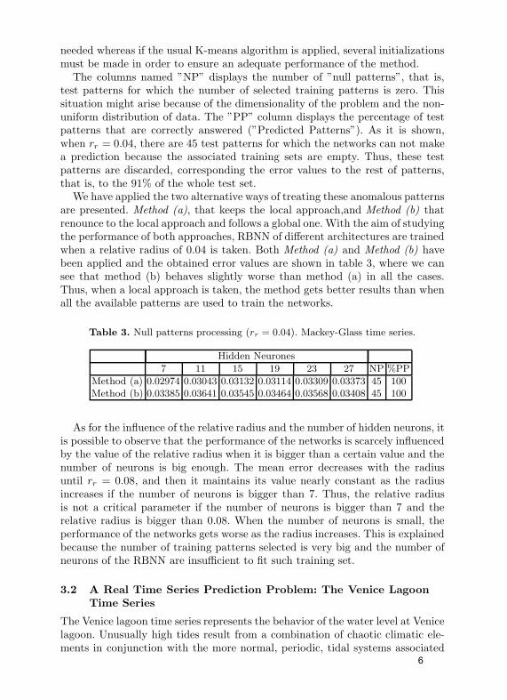
The columns named ”NP” displays the number of ”null patterns”, that is,test patterns for which the number of selected training patterns is zero. Thissituation might arise because of the dimensionality of the problem and the non-uniform distribution of data. The ”PP” column displays the percentage of testpatterns that are correctly answered (”Predicted Patterns”). As it is shown,when rr = 0.04, there are 45 test patterns for which the networks can not makea prediction because the associated training sets are empty. Thus, these testpatterns are discarded, corresponding the error values to the rest of patterns,that is, to the 91% of the whole test set.

We have applied the two alternative ways of treating these anomalous patternsare presented. Method (a), that keeps the local approach,and Method (b) thatrenounce to the local approach and follows a global one. With the aim of studyingthe performance of both approaches, RBNN of different architectures are trainedwhen a relative radius of 0.04 is taken. Both Method (a) and Method (b) havebeen applied and the obtained error values are shown in table 3, where we cansee that method (b) behaves slightly worse than method (a) in all the cases.Thus, when a local approach is taken, the method gets better results than whenall the available patterns are used to train the networks.

Table 3. Null patterns processing (rr = 0.04). Mackey-Glass time series.

Hidden Neurones7 11 15 19 23 27 NP %PP

Method (a) 0.02974 0.03043 0.03132 0.03114 0.03309 0.03373 45 100Method (b) 0.03385 0.03641 0.03545 0.03464 0.03568 0.03408 45 100

As for the influence of the relative radius and the number of hidden neurons, itis possible to observe that the performance of the networks is scarcely influencedby the value of the relative radius when it is bigger than a certain value and thenumber of neurons is big enough. The mean error decreases with the radiusuntil rr = 0.08, and then it maintains its value nearly constant as the radiusincreases if the number of neurons is bigger than 7. Thus, the relative radiusis not a critical parameter if the number of neurons is bigger than 7 and therelative radius is bigger than 0.08. When the number of neurons is small, theperformance of the networks gets worse as the radius increases. This is explainedbecause the number of training patterns selected is very big and the number ofneurons of the RBNN are insufficient to fit such training set.

3.2 A Real Time Series Prediction Problem: The Venice LagoonTime Series

The Venice lagoon time series represents the behavior of the water level at Venicelagoon. Unusually high tides result from a combination of chaotic climatic ele-ments in conjunction with the more normal, periodic, tidal systems associated

6

with a particular area. The most famous example of flooding in the Venice lagoonoccurred in November 1966 when, driven by strong winds, the Venice Lagoonrose by nearly 2 m. above the normal water level. That phenomenon is known as“high water” and many efforts have been made in Italy to develop systems forpredicting sea levels in Venice and mainly for the prediction of the high waterphenomenon [11].

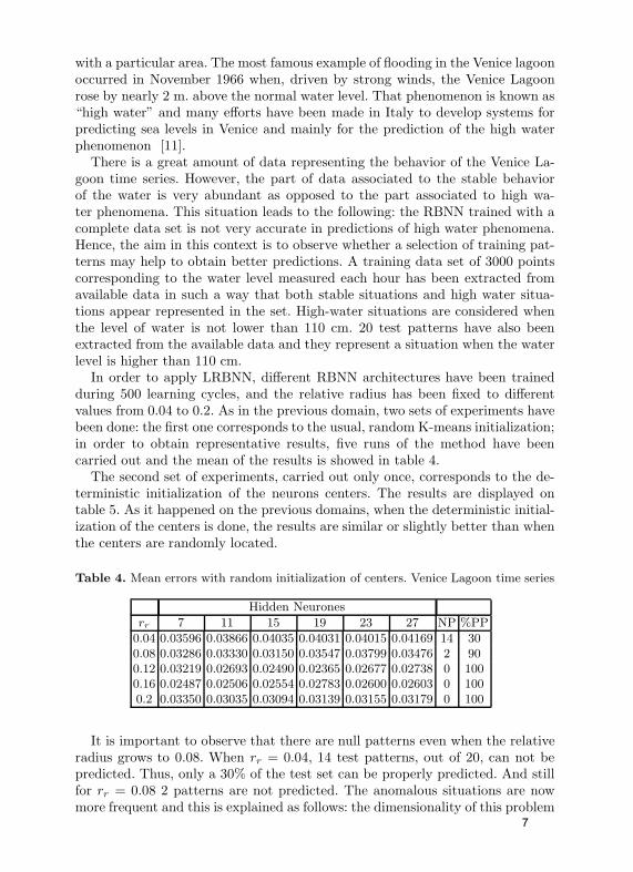
There is a great amount of data representing the behavior of the Venice La-goon time series. However, the part of data associated to the stable behaviorof the water is very abundant as opposed to the part associated to high wa-ter phenomena. This situation leads to the following: the RBNN trained with acomplete data set is not very accurate in predictions of high water phenomena.Hence, the aim in this context is to observe whether a selection of training pat-terns may help to obtain better predictions. A training data set of 3000 pointscorresponding to the water level measured each hour has been extracted fromavailable data in such a way that both stable situations and high water situa-tions appear represented in the set. High-water situations are considered whenthe level of water is not lower than 110 cm. 20 test patterns have also beenextracted from the available data and they represent a situation when the waterlevel is higher than 110 cm.

In order to apply LRBNN, different RBNN architectures have been trainedduring 500 learning cycles, and the relative radius has been fixed to differentvalues from 0.04 to 0.2. As in the previous domain, two sets of experiments havebeen done: the first one corresponds to the usual, random K-means initialization;in order to obtain representative results, five runs of the method have beencarried out and the mean of the results is showed in table 4.

The second set of experiments, carried out only once, corresponds to the de-terministic initialization of the neurons centers. The results are displayed ontable 5. As it happened on the previous domains, when the deterministic initial-ization of the centers is done, the results are similar or slightly better than whenthe centers are randomly located.

Table 4. Mean errors with random initialization of centers. Venice Lagoon time series

Hidden Neuronesrr 7 11 15 19 23 27 NP %PP

0.04 0.03596 0.03866 0.04035 0.04031 0.04015 0.04169 14 300.08 0.03286 0.03330 0.03150 0.03547 0.03799 0.03476 2 900.12 0.03219 0.02693 0.02490 0.02365 0.02677 0.02738 0 1000.16 0.02487 0.02506 0.02554 0.02783 0.02600 0.02603 0 1000.2 0.03350 0.03035 0.03094 0.03139 0.03155 0.03179 0 100

It is important to observe that there are null patterns even when the relativeradius grows to 0.08. When rr = 0.04, 14 test patterns, out of 20, can not bepredicted. Thus, only a 30% of the test set can be properly predicted. And stillfor rr = 0.08 2 patterns are not predicted. The anomalous situations are nowmore frequent and this is explained as follows: the dimensionality of this problem

7

Table 5. Mean errors with deterministic initialization. Venice Lagoon time series.

Hidden Neuronesrr 7 11 15 19 23 27 NP %PP

0.04 0.03413 0.03378 0.03328 0.03465 0.03404 0.03389 14 300.08 0.03181 0.03028 0.03062 0.03041 0.03148 0.03017 2 900.12 0.02967 0.02682 0.02269 0.02234 0.02235 0.02643 0 1000.16 0.02869 0.02398 0.02913 0.02059 0.02514 0.02552 0 1000.2 0.03769 0.02420 0.02411 0.02728 0.02288 0.03336 0 100

is higher than the former one because this series problem has been modeled as asix-dimension function; besides, there are regions of the input space whose datadensity is very low. The test set has been generated so that its data representthe high water situations, and the training examples which corresponds to theseunfrequent situations are very scarce. Thus, the null patterns processing methodspresented in this work are essential in the LRBNN model. Table 6 shows theerrors obtained when both methods (a) and (b) are applied if null patterns arefound. It is important to realize that, although it seems that the results are worsethan those seen on table 5, a 100% of the test patterns are properly predicted.

Table 6. Null patterns processing. Venice Lagoon time series.

Hidden Neuronesrr Meth 7 11 15 19 23 27 NP %PP

0.04 (a) 0.06042 0.06276 0.06292 0.06186 0.06330 0.06352 14 1000.04 (b) 0.09542 0.08128 0.06672 0.06239 0.06333 0.06500 14 1000.08 (a) 0.03685 0.03447 0.03011 0.03197 0.02792 0.03231 2 1000.08 (b) 0.04497 0.04382 0.03572 0.03407 0.03266 0.03441 2 100

In this domain, the differences between both methods are significant, speciallywhen the relative radius is 0.04. In this case, 14 null patterns are found, that is,70% of the whole test set. We can appreciate that method (a) achieves lower er-rors that method (b). Thus, when a lazy learning approach is applied the result isbetter than when the RBNN are trained with all the available training patterns.

It is possible to observe that, as in previous cases, when the relative radiusis small, mean errors are high, due to the shortage of selected training patterns,and as the relative radius increases, the mean error decreases and then it doesnot change significatively. Thus, as it happened with the previous domains, therelative radius is not a critical parameter if the number of neurons and therelative radius are bigger enough.

3.3 Lazy Learning Versus Global Learning

In order to compare the lazy learning strategy (LRBNN) with the traditional one,RBNN with different number of hidden neurons (from 5 to 150) have been trained,

8

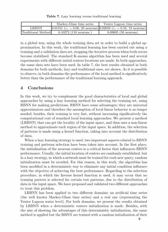
Table 7. Lazy learning versus traditional learning

Mackey-Glass time series Venice Lagoon time seriesLRBNN 0.01551 (rr = 0.08, 23 neurons) 0.02059 (rr = 0.16, 19 neurons)

Traditional Method 0.10273 (110 neurons ) 0.09605 (50 neurons)

in a global way, using the whole training data set in order to build a global ap-proximation. In this work, the traditional learning has been carried out using atraining and a validation data set, stopping the iterative process when both errorsbecome stabilized. The standard K-means algorithm has been used and severalexperiments with different initial centers locations are made. In both approaches,the same data sets have been used. In table 7, the best results obtained in bothdomains for both methods, lazy and traditional ones, are shown. As it is possibleto observe, in both domains the performance of the local method is significativelybetter than the performance of the traditional learning approach.

4 Conclusions

In this work, we try to complement the good characteristics of local and globalapproaches by using a lazy learning method for selecting the training set, usingRBNN for making predictions. RBNN have some advantages: they are universalapproximators and therefore the assumption of local linear behavior is no longerneeded; besides, their training is very fast, without increasing significatively thecomputational cost of standard local learning approaches. We present a method(LRBNN) that can get the locality of the input space, and then uses a non-linearmethod to approximate each region of the input space. In addition, the selectionof patterns is made using a kernel function, taking into account the distributionof data.

When a lazy learning strategy is used, two important aspects related to RBNNtraining and patterns selection have been taken into account. In the first place,the initialization of the neurons centers is a critical factor that influences RBNNperformance. Usually, the initial location of centers are randomly established, butin a lazy strategy, in which a network must be trained for each new query, randominitialization must be avoided. For this reason, in this work, the algorithm hasbeen modified in a deterministic way to eliminate any initial condition influencewith the objective of achieving the best performance. Regarding to the selectionprocedure, in which the Inverse kernel function is used, it may occur that notraining pattern is selected for certain test patterns, due to the distribution ofdata in the input space. We have proposed and validated two different approachesto treat this problem.

LRBNN has been applied to two different domains: an artificial time series(the well known Mackey-Glass time series) and a real one (representing theVenice Lagoon water level). For both domains, we present the results obtainedby LRBNN when a deterministic centers initialization is made. Besides, withthe aim of showing the advantages of this deterministic initialization, the samemethod is applied but the RBNN are trained with a random initialization of their

9

centers. We show the mean results of several random initializations. As we saidbefore, LRBNN provides two alternative ways of guarantying the selection oftraining examples for all the query instances. When the use of these alternativemethods is necessary, the obtained results are also showed. Finally, LRBNNperformance is compared with the performance of RBNN trained using a globalapproach, that is, using the whole training set.

The results obtained by LRBNN improves significatively the ones obtained byRBNN trained in a global way. Besides, the proposed deterministic initializationof the neurons centers produces similar or slightly better results than the usualrandom initialization, being thus preferable because only one run is necessary.Moreover, the method is able to predict 100% of the test patterns, even inthose extreme cases when no train examples would be selected using the normalselection method. The experiments show that the relative radius, parameter ofthe method, is not a critical factor because if it reaches a minimum value andthe network has a sufficient number of neurons, the error on the test set keepsits low value relatively constant.

Thus, we can conclude that the combination of lazy learning and RBNN, canproduce significant improvements in some domains.

Acknowledgments. This article has been financed by the Spanish foundedresearch MEC project OPLINK::UC3M, Ref: TIN2005-08818-C04-02

References

1. D.W. Aha, D. Kibler, and M.K. Albert. Instance-based learning algorithms. Ma-chine Learning, 6:37–66, 1991.

2. L. Bottou and V. Vapnik. Local learning algorithms. Neural Computation,4(6):888–900, 1992.

3. C.G. Atkenson, A.W. Moore, and S. Schaal. Locally weighted learning. ArtificialIntelligence Review, 11:11–73, 1997.

4. B.V. Dasarathy (Editor). Nearest neighbour(NN) norms: NN pattern classificationtechniques. IEEE Computer Society Press, 1991.

5. J. Ghosh and A. Nag. An Overview of Radial Basis Function Networks. R.J.Howlett and L.C. Jain (Eds). Physica Verlag, 2000.

6. J.E. Moody and C. Darken. Fast learning in networks of locally tuned processingunits. Neural Computation, 1:281–294, 1989.

7. J. Park and I.W. Sandberg. Universal approximation and radial-basis-functionnetworks. Neural Computation, 5:305–316, 1993.

8. J.M. Valls, I.M. Galvan, and P. Isasi. Lazy learning in radial basis neural networks: away of achieving more accurate models. Neural Processing Letters, 20:105–124, 2004.

9. D. Wettschereck and T. Dietterich. Improving the perfomance of radial basisfunction networks by learning center locations. Advances in Neural InformationProcessing Systems, 4:1133–1140, 1992.

10. L. Yingwei, N. Sundararajan, and P. Saratchandran. A sequential learning schemefor function approximation using minimal radial basis function neural networks.Neural Computation, 9:461–478, 1997.

11. J.M. Zaldıvar, E. Gutierrez, I.M. Galvan, F. Strozzi, and A. Tomasin. Forecastinghigh waters at Venice Lagoon using chaotic time series analysis and nonlinearneural networks. Journal of Hydroinformatics, 2:61–84, 2000.

10