Final version, Contributed article submitted to Neural Networks, section Engineering and Design

Sensitivity Analysis Applied to the Construction

of Radial Basis Function Networks

D. Shi1, D. S. Yeung2 and J. Gao3

1School of Computer Engineering, Nanyang Technological University, Singapore 639798

2Department of Computing, Hong Kong Polytechnic University, Hung Hom, Kowloon, Hong Kong

3School of Mathematics, Statistics and Computer Science, University of New England, Australia

Contact author: Dr. Daming Shi, School of Computer Engineering,

Nanyang Technological University, Singapore 639798

Tel: +65 6790 6245 Fax: +65 6792 6559 Email: asdmshi@ntu.edu.sg

29 March 2005

1

Sensitivity Analysis Applied to the Construction of

Radial Basis Function Networks

D. Shi1*, D. S. Yeung2 and J. Gao3

1School of Computer Engineering, Nanyang Technological University, Singapore 639798

2Department of Computing, Hong Kong Polytechnic University, Hung Hom, Kowloon, Hong Kong

3School of Mathematics, Statistics and Computer Science, University of New England, Australia

( *Corresponding author, Email: asdmshi@ntu.edu.sg)

Abstract

Conventionally, a radial basis function (RBF) network is constructed by obtaining

cluster centers of basis function by maximum likelihood learning. This paper proposes

a novel learning algorithm for the construction of radial basis function using

sensitivity analysis. In training, the number of hidden neurons and the centers of their

radial basis functions are determined by the maximization of the output’s sensitivity

to the training data. In classification, the minimal number of such hidden neurons with

the maximal sensitivity will be the most generalizable to unknown data. Our

experimental results show that our proposed sensitivity-based RBF classifier

outperforms the conventional RBFs and is as accurate as support vector machine

(SVM). Hence, sensitivity analysis is expected to be a new alternative way to the

construction of RBF networks.

Keywords: Sensitivity analysis, radial basis function neural network, orthogonal least

square learning, network pruning

2

1. Introduction

As one of the most popular neural network models, radial basis function (RBF)

network attracts lots of attentions on the improvement of its approximate ability as

well as the construction of its architecture. Bishop (1991) concluded that an RBF

network can provide a fast, linear algorithm capable of representing complex non-

linear mappings. Park and Sandberg (1993) further showed that RBF network can

approximate any regular function. In a statistical sense, the approximate ability is a

special case of statistical consistency. Hence, Xu et al. (1994) presented upper bounds

for the convergence rates of the approximation error of RBF networks, and proved

constructively the existence of a consistent estimator point-wise and L2 convergence

rates of the best consistent estimator for RBF networks. Their results can be a guide to

optimize the construction of an RBF network, which includes the determination of the

total number of radial basis functions along with their centers and widths.

There are three ways to construct an RBF network, namely, clustering, pruning and

critical vector learning. Bishop (1991) and Xu (1998) follow the clustering method, in

which the training examples are grouped and then each neuron is assigned to a cluster.

The pruning method, such as Chen et al. (1991) and Mao (2002), creates a neuron for

each training example and then to prune the hidden neurons by example selection.

The critical vector learning method, exemplified by Schokopf et al. (1997) constructs

an RBF with the critical vectors, rather than cluster centers.

3

Moody and Darken (1989) located optimal set of centers using both the k-means

clustering algorithm and learning vector quantization. The drawback of this method is

that it considers only the distribution of the training inputs, yet the output values

influence the positioning of the centers. Bishop (1991) introduced the Expectation-

Maximization (EM) algorithm to optimize the cluster centers with two steps:

obtaining initial centers by clustering and optimization of the basis functions by

applying the EM algorithm. Such a treatment actually does not perform a maximum

likelihood learning but a suboptimal approximation. Xu (1998) extended the model

for mixture of experts to estimate basis functions, output neurons and the number of

basis functions all together. The maximum likelihood learning and regularization

mechanism can be further unified to his established Bayesian Ying Yang (BYY)

learning framework (Xu, 2004a, 2004b, 2004c), in which any problem can be

decomposed into Ying space or invisible domain (e.g., the hidden neurons in RBFs),

and Yang space or visible domain (e.g., the training examples in RBFs), and the

invisible/unknown parameters can be estimated through harmony learning between

these two domains.

Chen et al. (1991) proposed orthogonal least square (OLS) learning to determine the

optimal centers. The OLS combines the orthogonal transform with the forward

regression procedure to select model terms from a large candidate term set. The

advantage of employing orthogonal transform is that the responses of the hidden layer

neurons are decorrelated so that the contribution of individual candidate neurons to

the approximation error reduction can be evaluated independently. However, the

original OLS learning algorithm lacks generalization and global optimization abilities.

Mao (2002) employed OLS to decouple the correlations among the responses of the

4

hidden units so that the class separability provided by individual RBF neurons can be

evaluated independently. This method can select a parsimonious network architecture

as well as centers providing large class separation.

The common feature of all the above methods is that the radial basis function centers

are a set of the optimal cluster centers of the training examples. Schokopf et al. (1997)

calculated support vectors using a support vector machine (SVM), and then used

these support vectors as radial basis function centers. Their experimental results

showed that the support-vector-based RBF outperforms conventional RBFs.

Although the motivation of these researchers was to demonstrate the superior

performance of a full support vector machine over either conventional or support-

vector-based RBFs, their idea of critical vector learning is worth borrowing.

This paper proposes a novel approach to determining the centers of RBF networks

based on sensitivity analysis. The remainder of this paper is organized as follows: In

section 2, we describe the concepts of sensitivity analysis. In section 3, the most

critical vectors are obtained by OLS in terms of sensitivity analysis. Section 4

contains our experiments and Section 5 offers our conclusions.

2. Sensitivity Analysis on Neural Networks

Sensitivity is initially investigated for the construction of a network prior to its design,

since problems (such as weight perturbation, which is caused by machine imprecision

5

and noisy input) significantly affect network training and generalization (Widrow,

1960). Stevenson (1990) established sensitivity analysis to weight error and derive an

analytical expression for the probability of error in Madaline. Typically, one can

simulate hardware imprecision by introducing perturbation on weight and input to

measure the sensitivity. Zurada et al. (1997) extended this idea of sensitivity analysis

to network pruning.

There are two different methods to measure sensitivity, one is noise-to-signal ratio,

the other is expectation of output error. Sensitivity analysis is conducted by measuring

the response of the network when parameter perturbations are introduced

intentionally.

Treating all network inputs, weights, input perturbations, and weight perturbations as

random variables, Piche (1995) defined sensitivity as the noise-to-signal-ratio (NSR)

of the output layer:

2

2

2

2

2

2 4

w

w

x

x

y

yNSRσσ

σσ

πσσ

∆∆∆ +== , (1)

where , , , , and refer to the variances of output y, inputs x,

weights w, output error , input perturbation

2yσ 2

xσ 2wσ 2

y∆σ2x∆σ

2w∆σ

y∆ x∆ and weight perturbation ,

respectively. Piche’s stochastic model is not generally valid because: (1) All neurons

in the same layer are assumed to have the same activation function, but this is not the

case in some network models. (2) To satisfy the central limit theorem, the number of

neurons in hidden layers is assumed to be large. (3) Weight perturbations are assumed

w∆

6

to be very small, but this would be too restrictive for network training. To address

these problems, Yeung and Sun (2002) generalized Piche (1995)’s work in two

significant ways: (1) No restriction on input and output perturbation, which widens

the application areas of sensitivity analysis; (2) The commonly--used activation

functions are approximated by a general function expression whose coefficient will be

involved in the sensitivity analysis. This treatment provides a way to sensitivity

analysis on activation functions.

Zeng and Yeung ( 2001, 2003) proposed a quantified measure and its computation for

the sensitivity of the MLP to its input perturbation. The sensitivity of a single

neuron i in layer l is defined as the mathematical expectation of the absolute value of

its output deviation caused by the perturbation

lis

lX∆ :

( )⎟⎟⎟

⎠

⎞

⎜⎜⎜

⎝

⎛−

⎟⎟⎟

⎠

⎞

⎜⎜⎜

⎝

⎛∆+= l

ill

illl

i WfWfEs **)(_____

XXX (2)

A bottom-up approach was adopted. After the sensitivities of single neurons are

calculated, the sensitivity of the entire MLP network will be computed. Some

applications of the MLP, such as improving error tolerance, measuring generalization

ability, and pruning the network architecture, would benefit from their theoretical

study. However, this method would be even more useful if it took into considerations

of correlation among training examples.

7

3. Construction of RBF Networks with Sensitivity Analysis

An RBF classifier is a three-layer neural network model, in which an N-dimensional

input vector x=(x1 x2 … xN) is broadcast to each of K neurons in the hidden layer.

Each hidden neuron produces an activation function, typically a Gaussian kernel:

⎟⎟

⎠

⎞

⎜⎜

⎝

⎛ −−= 2

2

2exp

i

iih

σcx

, i=1,2,…,K, (3)

where and are the center and width of the Gaussian basis function of the ith

hidden unit, respectively. The units in the output layer have interconnections with all

the hidden units. The jth output neuron has the form:

ic 2iσ

∑= ⎟

⎟

⎠

⎞

⎜⎜

⎝

⎛ −−==

K

i i

iijjj wf

12

2

2exp)(

σcx

hwx (4)

where h=(h1 h2 … hK) is the input vector from the hidden layer, and the is the

interconnection weight between the jth output neuron and the ith hidden neuron.

ijw

In this section, RBF classifier’s sensitivity is defined as the mathematical expectation

of the square of output deviations caused by the perturbation of RBF centers. An

algorithm will be given that can be used to select critical vectors.

8

3.1 RBF Classifiers’ Sensitivity to the Kernel Function Centers

We use symbols and ic iσ to denote the values of center and width of the ith hidden

neuron under a perturbation. Then the deviation resulting from this perturbation is:

∑∑== ⎟

⎟

⎠

⎞

⎜⎜

⎝

⎛ −−−

⎟⎟

⎠

⎞

⎜⎜

⎝

⎛ −−=−=∆

K

i i

iij

K

i i

iijjjj wwy

12

2

12

2

2exp

ˆ2ˆ

expˆˆˆσσcxcx

hwhw (5)

Here, are the centers deviated from the centers under the perturbations,

and the interconnection weights under the perturbations are

iii ccc ∆+=ˆ

jjj www ∆+=ˆ , where

can be calculated using a pseudo matrix inversion, or data training. Although

there are ways to specify RBF widths, such as (Xu et al. 2004), the most common

method for selecting RBF widths is to make all of them equal to a constant value

depending on the prior knowledge of the given application. With pre-defined RBF

widths, we just focus on the perturbations on the centers and their interconnection

weights in this research. The perturbation on the ith RBF center and the weights

connected to the jth output, and

jw

ic∆ jw∆ , can be generated following a Gaussian

distribution with 0 means and variances icσ ,

jwσ , respectively:

⎟⎟

⎠

⎞

⎜⎜

⎝

⎛ ∆∆−=∆

⎟⎟⎠

⎞⎜⎜⎝

⎛ ∆∆−=∆

2

2

2exp

)2(1)(

2exp

)2(1)(

jj

ii

jTj

Kj

iTi

Ni

p

p

ww

cc

www

ccc

σπσ

σπσ (6)

where N is the dimension of the input x, K is the number of RBF centers.

9

The RBF centers will be selected recursively in the next subsection. To make the

sensitivity analysis cater for the construction of RBF networks, a recursive definition

of sensitivity is given below. At the Kth time, suppose there are a number (K –1) of

RBF centers fixed already, the newcomer is observed. Hence, the jth output

neuron’s sensitivity to the current number K of RBF centers is defined as the

mathematical expectation of (square of output deviations caused by the

perturbations of RBF centers) with respect to all

ic

2)( jy∆

ic∆ and the training example set

, which is expressed as { }LllD 1== x

)(KjS ])[( 2

jyE ∆=

= wcccxccx

cwx

∆∆⎟⎟

⎠

⎞

⎜⎜

⎝

⎛ ∆−−−

∆−−−∆∆∫ ∑∑

=∈

ddwwppn

nnl

m

mmlnj

K

nmmj

Dl

2

2

2

2

1, 22expˆˆ)()(

σσ

wcccxccx

cwx

∆∆⎟⎟

⎠

⎞

⎜⎜

⎝

⎛ ∆−−−

∆−−−∆∆− ∫ ∑∑

=∈

ddwwppn

nnl

m

mmlnj

K

nmmj

Dl

2

2

2

2

1, 22expˆ)()(2

σσ

wcccxccx

cwx

∆∆⎟⎟

⎠

⎞

⎜⎜

⎝

⎛ ∆−−−

∆−−−∆∆+ ∫ ∑∑

=∈

ddwwppn

nnl

m

mmlnj

K

nmmj

Dl

2

2

2

2

1, 22exp)()(

σσ

= (7) 321 2 III +−

where , and are figured out by integrating over 1I 2I 3I c∆ and w∆ , so

= 1I( )

( ) ⎟⎟

⎠

⎞

⎜⎜

⎝

⎛

+

−−

+

−−

++∑∑

≠=∈ )(2)(2exp

))((22

2

22

2

2222

22

;1, nmnm

l n

nl

m

mlN

nm

N

nmnj

K

nmnmmj

Dww

cccc

x

cxcxσσσσσσσσ

σσ

( )

( )∑∑=∈ ⎟

⎟

⎠

⎞

⎜⎜

⎝

⎛

+

−−

+++

K

m m

mlN

m

N

mmj

D mm

j

l

w1

22

2

22

222

)2(exp

)2()(

cc

wx

cxσσσσ

σσ ,

10

and similarly, we have

= 2I( )

( ) ⎟⎟

⎠

⎞

⎜⎜

⎝

⎛ −−

+

−−

+∑∑

=∈2

2

22

2

22

2

1, 2)(2exp

)( n

nl

m

mlN

m

N

mnj

K

nmmj

D mm

l

wwσσσσσ

σ cxcx

cc

x,

= 3I⎟⎟

⎠

⎞

⎜⎜

⎝

⎛ −−

−−∑∑

=∈2

2

2

2

1, 22exp

n

nl

m

mlnj

K

nmmj

Dww

lσσ

cxcx

x

.

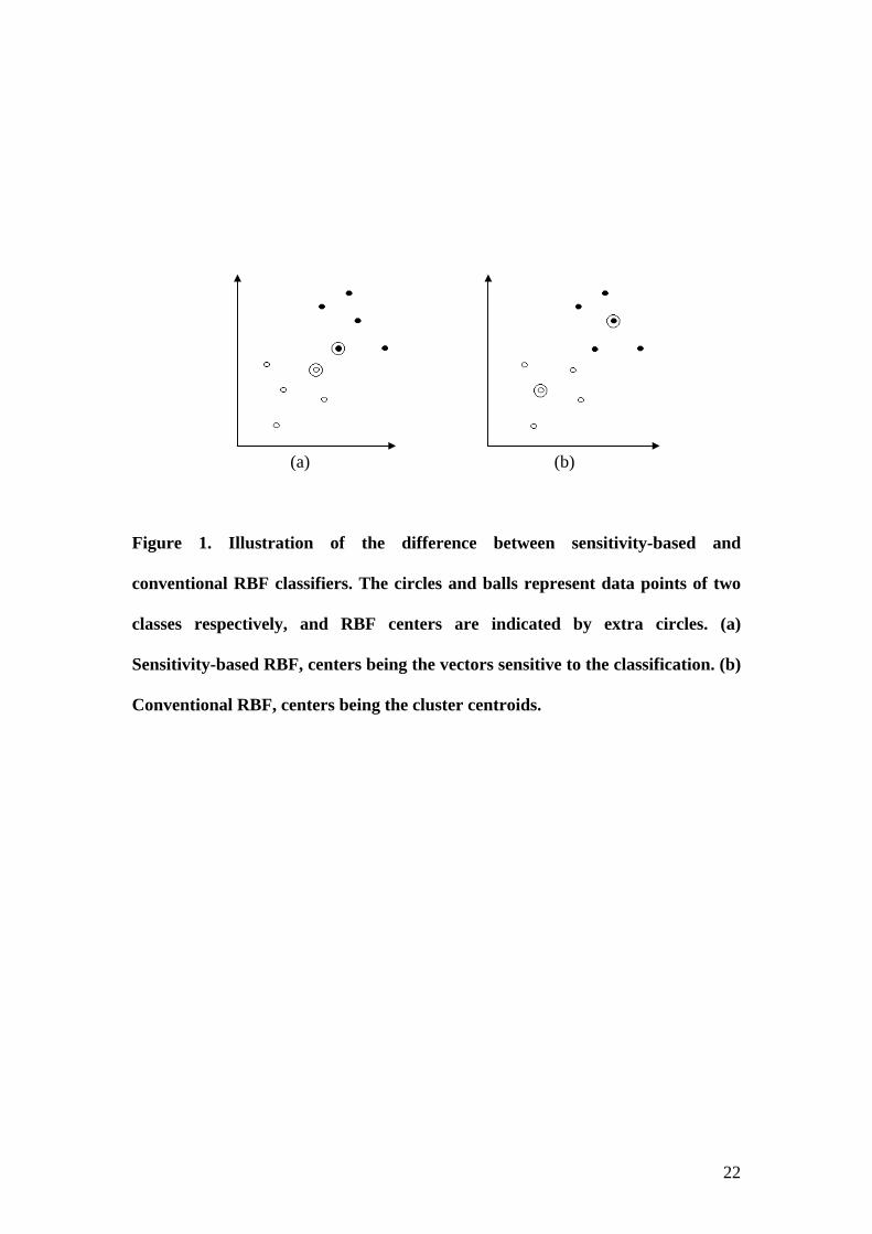
Similar to the comparison between support-vector-based and clustering-based RBF

networks in Scholkopf et al. (1997), the difference between the sensitivity-based and

the conventional RBF networks can be shown in Figure 1.

[Figure 1] 3.2 Orthogonal Least Square Transform

The most critical vectors can be found by equation (7). However, the RBF centers

cannot be determined by sensitivity measure only, because some of critical vectors

may be correlated. The OLS (Chen et al. 1991) can alleviate this problem of

redundant or correlated centers.

11

Let Y=(y1, y2… yL)T be the output matrix corresponding to all the number L of

training examples, yi (i=1,2,…,L) an M-dimensional vector, denoting number M of

output units. We have

Y=HW=(QA)W (8)

Where Y, H, W are MLLLML ××× ,, matrices, respectively. The selection of RBF

centers is equivalent to the selection of the most critical columns of H. The matrix H

can be decomposed into QA, where Q is an LL× matrix with orthogonal columns

[q1, q2, …, qL], and A is an upper triangular matrix as follows: LL×

⎥⎥⎥⎥⎥⎥

⎦

⎤

⎢⎢⎢⎢⎢⎢

⎣

⎡

=

LLL

L

hh

hhhhh

LL

M

MM

M

L

1

1212

11211

H , . (9)

⎥⎥⎥⎥⎥⎥

⎦

⎤

⎢⎢⎢⎢⎢⎢

⎣

⎡

=

−

10010

010

1

)1(

23

112

LL

M

MOM

M

LL

LL

L

a

aaa

A

Only one column of H is orthogonalized in each iteration. At the Kth iteration, one

column is made orthogonal to each of the K-1 previously orthogonalized columns.

The computational procedure can be represented as follows (Chen et al. 1991):

⎪⎪⎪⎪

⎩

⎪⎪⎪⎪

⎨

⎧

−=

=

=

∑−

=

1

1

11

,

,

K

iiiKKK

i

KTi

ik

a

a

hhq

qhq

hq

Ki <≤1 , (10)

12

then the RBF centers are selected by sorting these columns.

3.3 Critical Vector Selection

Let denote the sensitivity of the previous (K-1) RBF centers and a candidate

RBF center which is corresponding to at the Kth time, where .

)()(i

K cS

ic iq Li ≤≤1

Substitute any interconnection weight in equations (5) and (7) by:

∑=

⋅=L

lijli

Kij waw

1

)( , (11)

and calculate the sensitivity for all the possible K-center RBF networks. Let

denote the orthogonal matrix at the Kth time, then the columns in are sorted in

the order:

)(KQ

)(KQ

)()()( )(2

)(1

)(L

KKK cScScS ≥≥≥ L . (12)

A formal statement of the algorithm for the selection of critical vectors is given as

follows:

STEP 1. Initialization. Form the matrix H in equation (8) by the RBF function

responses of all the training examples.

STEP 2. First critical vector neuron selection. Calculate sensitivity of each column

of H with equation (7). The column that provides the maximum sensitivity is selected

as the first column of matrix . Calculate the classification error Err)1(Q (1) with the

selected RBF center. Let K=2.

13

STEP 3. Orthogonalization and critical vector selection. Orthogonalize all

remaining columns of H with all the columns of using equation (10). )1( −KQ

STEP 4. Each training example, , is a candidate for the Kth RBF center, which is

corresponding to the orthogonalized column , (

ic

iq LiK ≤≤ ). Calculate

interconnection weights using a pseudo matrix inversion and compute the sensitivity

of the previous (K-1) RBF centers with each candidate center with the

weights updated by equation (11). Sort the columns in with equation (12), and

the one yielding the maximum sensitivity is selected as the Kth column of .

Calculate the classification error Err

)()(i

K cS

)(KQ

)(KQ

(K) with the selected RBF centers.

STEP 5. If (Err(K)- Err(K-1) ) is smaller than a predefined threshold, go to STEP 7.

STEP 6. K++, go to STEP 3.

STEP 7. End.

The critical vectors corresponding to the first K columns in will be selected as

hidden neurons.

)(KQ

4. Experiments and Results

Our experiments were conducted on 2 datasets from UCI Repository (Blake and

Merz, 1998), and 2 datasets from the Statlog collection (Michie et al. 1994). The

experiments are described as follows:

14

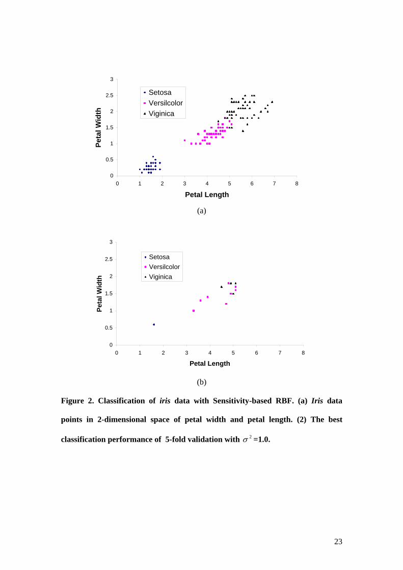
UCI Iris Plants (iris). This is the best--known database in the pattern recognition

literature. The dataset contains 3 classes referring to 3 types of iris plant: Setosa,

Versicolour and Virginica, respectively. One class is linearly separable from the

others, but the other two classes are not linearly separable from each other. There are

150 instances (50 in each class), which are described by 4 attributes, sepal length,

sepal width, petal length and petal width. 5-fold cross validation is conducted on the

entire data set. Figure 2(a) shows the whole set of training examples, and Figure 2(b)

shows the best score with the number of critical vectors being 13.

UCI Glass Identification (glass). This study is motivated by criminological

investigation using the glass as evidence at the scene of the crime. There are 214 of

instances from 6 classes. The 9 features include glass material information, such as

sodium, silicon, or iron. 5-fold cross validation is conducted on the entire dataset and

the best score is reported.

Statlog Satellite Images (satimage). There are 4435 training examples and 2000

testing examples in this dataset. Each instance consists of the pixel values in the 4

spectral bands of each of the 9 pixels in the 33× neighborhood, that are contained in

a frame of a Landsat satellite image. The objective is to classify the central pixels into

6 attributes, such as red soil, or cotton crop.

Statlog Letters (letter). This dataset comprises a collection of 20,000 stimuli,

consisting of 26 categories of capital English letters on different fonts. Each stimulus

was converted into 16 primitive numerical attributes, such as statistical moments and

15

edge counts. The first 15000 items are chosen to be training examples and remaining

5000 items to be testing examples.

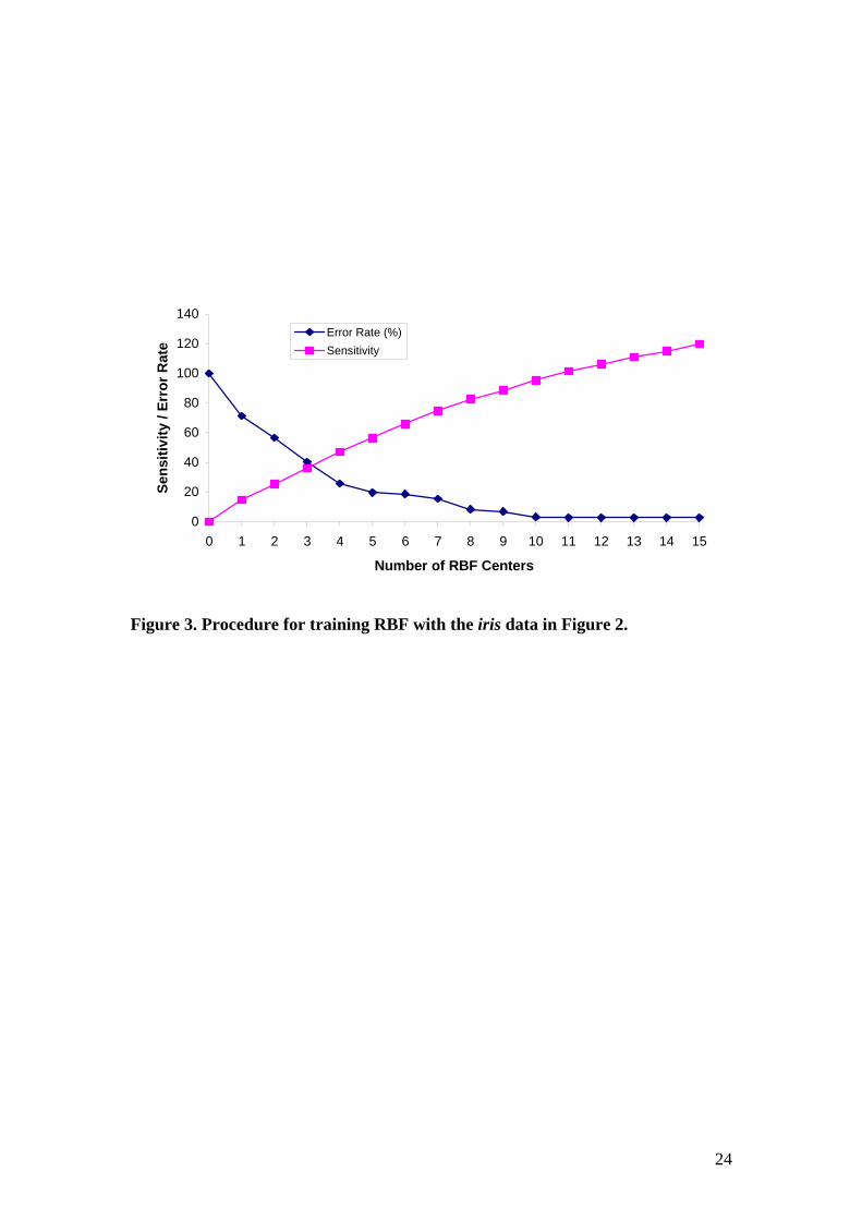
[Figure 2] Figure 3 shows the procedure for training RBF with iris data in figure 2. It can be

seen that the output error decreases with respect to the number of critical vectors,

while the sensitivity increases. However, the change of output error turns out to be flat

earlier than that of the sensitivity.

[ Figure 3 ] Table 1 compares the classification accuracies achieved with the proposed sensitivity-

based RBF (SenV-RBF), support vector machine (Hsu and Lin, 2002), conventional

RBF (Bishop, 1991), and decision tree C4.5 (Quinlan, 1993). The training examples

and testing examples for all the methods are the same as those chosen for our

proposed SenV-RBF.

[Table 1]

16

As table 1 shows, data classification based on the proposed sensitivity-based RBF

classifier performs better than the conventional RBF and the C4.5. The exception to

this, glass, indicates that from case to case the Gaussian kernel function may have

some blind spots. As also shown in Table 1, the sensitivity-based RBF is time-

consuming in training. Firstly, this is not a problem, as it provides a very fast and

accurate classification in run-time, our area of concern. Secondly, SenV-RBF enjoys

shorter computational time for multiple-class problems than SVM. It can also be seen

that both the sensitivity-based RBF and the SVM achieve basically the same level of

accuracy, but the former performs better in multiple-class problems and more robust

against noisy data.

5. Conclusions and Future Work

The conventional approach to constructing an RBF network is to search for the

optimal cluster centers among the training examples. This paper proposes a novel

approach to RBF construction that uses critical vectors selected by sensitivity

analysis. Sensitivity is defined as the expectation of the square of output deviation

caused by the perturbation of RBF centers. In training, orthogonal least square

incorporated with a sensitivity measure is employed to search for the optimal critical

vectors. In classification, the selected critical vectors will take on the role of the RBF

centers. Our experimental results show that our proposed RBF classifier performs

better than the conventional RBFs and C4.5. The sensitivity-based RBF can achieve

17

the same level of accuracy as SVM, but strikes a balance between critical vector

learning and robustness against noisy data.

Our future work includes the development of a decomposition method for large scale

classification problems, as well as the optimization of RBF widths integrated into

sensitivity analysis.

Acknowledgements The authors would like to express their gratitude to the reviewers, whose valuable

comments are very helpful in revising the paper. The first author thanks Fei Chen for

the help in the experiments.

References

Bianchini, M., Frasconi, P. & Gori, M. (1995). Learning without local minima in radial basis function

networks, IEEE Transactions on Neural Networks, 6(3):749-756.

Bishop, C. M. (1991). Improving the generalization properties of radial basis function neural networks,

Neural Computation, 3(4):579-581.

Bishop, C. M. (1995). Training with noise is equivalent to Tikhonov regularization, Neural

Computation, 7(1):108-116.

Blake, C. L., & Merz, C. J. (1998). UCI Repository of machine learning databases. School of

Information and Computer Science, University of California, Irvine, CA. [Online]. Available:

http://www.ics.uci.edu/~mlearn/MLRepository.html.

18

Chen, S., Crown, C. F., & Grant, P. M. (1991). Orthogonal least squares learning algorithms for radial

basis function networks, IEEE Transactions on Neural Networks, 2(2):302-309.

Choi, J. Y., & Choi, C. H. (1992). Sensitivity analysis of multilayer perceptron with differentiable

activation functions, IEEE Transactions on Neural Networks, 3(1):101-107, 1992.

Kadirkamanathan, V., & Niranjan, M. (1993). A function estimation approach to sequential learning

with neural networks, Neural Computation, 5(6):954-975.

Hsu, C. W., & Lin, C. J. (2002). A comparison of methods for multi-class support vector machines,

IEEE Transactions on Neural Networks, 13(2):415-425.

Mao, K. Z. (2002). RBF neural network center selection based on fisher ratio class separability

measure, IEEE Transactions on Neural Networks, 13(5):1211-1217.

Michie, D., Spiegelhalter, D. J., & Taylor, C. C. (1994). Machine learning, neural and statistical

classification. [Online]. Available: http://www.liacc.up.pt/ML/statlog/datasets.html.

Moody, J., & Darken, C. J. (1989). Fast learning in networks of locally-tuned processing units, Neural

Computation, 1:281-294.

Park, J., & Sandberg, I. W. (1993). Approximation and radial basis function networks, Neural

Computation, 5:305-316.

Piche, S. W. (1995). The selction of Weight Accuracies for Madalines, IEEE Transactions on Neural

Networks, 6(2):432-445, 1995.

Quinlan, J. R. (1993). C4.5: Programs for Machine Learning. San Mateo, CA: Morgan Kaufmann.

19

Scholkopf, B., Sung, K. K., Burges, C. J. C., Girosi, F., Niyogi, P., Poggio, T., & Vapnik, V. (1997).

Comparing support vector machines with Gaussian kernels to radial basis function classifiers, IEEE

Transactions on Signal Processing, 45(11):2758-2765.

Stevenson, M., Winter, R., & Widrow, B. (1990). Sensitivity of feedforward neural networks to weight

errors, IEEE Transactions on Neural Networks, 1(1):71-80.

Wang, Z., & Zhu, T. (2000). An efficient learning algorithm for improving generalization performance

of radial basis function neural networks, Neural Networks, 13(4):545-553.

Widrow, B., (1960), Adaptive switching circuits, in IREWESCON Convention Record, pp. 96-104,

New York.

Xu, L., Krzyzak, A. & Yuille A. (1994). On radial basis function nets and kernel regression: statistical

consistency, convergence rates, and receptive field size, Neural Networks, 7(4):609-628.

Xu, L., (1998). RBF nets, mixture experts, and Bayesian Ying-Yang learning, Neuocomputing,

19:223-257.

Xu, L. (2004a), Bayesian Ying Yang Learning (I): A Unified Perspective for Statistical Modeling, In:

Intelligent Technologies for Information Analysis, N. Zhong and J. Liu (eds), Springer, pp.615-659.

Xu, L. (2004b), Bayesian Ying Yang Learning (II): A New Mechanism for Model Selection and

Regularization, In: Intelligent Technologies for Information Analysis, N. Zhong and J. Liu (eds),

Springer, pp.661-706.

Xu, L. (2004c), Advances on BYY Harmony Learning: Information Theoretic Perspective, Generalized

Projection Geometry, and Independent Factor Auto-determination, IEEE Trans on Neural Networks,

15(4):885-902.

20

Yeung, D. S., & Sun, X. (2002). Using function approximation to analyze the sensitivity of MLP with

antisymmetric squashing activation function, IEEE Transactions on Neural Networks, 13(1):34-44.

Zeng, X., & Yeung, D. S. (2001). Sensitivity analysis of multilayer perceptron to input and weight

perturbation, IEEE Transactions on Neural Network, 12(6):1358-1366.

Zeng, X., & Yeung, D. S. (2003). A quantified sensitivity measure for multilayer perceptron to input

perturbation, Neural Computation, 15:183-212.

Zurada, J. M., Malinowski, A., & Usui, S. (1997). Perturbation method for deleting redundant inputs of

perceptron networks. Neurocomputing, 14(2):177-193.

21

(a) (b)

Figure 1. Illustration of the difference between sensitivity-based and

conventional RBF classifiers. The circles and balls represent data points of two

classes respectively, and RBF centers are indicated by extra circles. (a)

Sensitivity-based RBF, centers being the vectors sensitive to the classification. (b)

Conventional RBF, centers being the cluster centroids.

22

0

0.5

1

1.5

2

2.5

3

0 1 2 3 4 5 6 7 8

Petal Length

Peta

l Wid

thSetosaVersilcolorViginica

(a)

0

0.5

1

1.5

2

2.5

3

0 1 2 3 4 5 6 7 8

Petal Length

Peta

l Wid

th

SetosaVersilcolorViginica

(b)

Figure 2. Classification of iris data with Sensitivity-based RBF. (a) Iris data

points in 2-dimensional space of petal width and petal length. (2) The best

classification performance of 5-fold validation with =1.0. 2σ

23

0

20

40

60

80

100

120

140

0 1 2 3 4 5 6 7 8 9 10 11 12 13 14 15

Number of RBF Centers

Sens

itivi

ty /

Erro

r Rat

e

Error Rate (%)Sensitivity

Figure 3. Procedure for training RBF with the iris data in Figure 2.

24

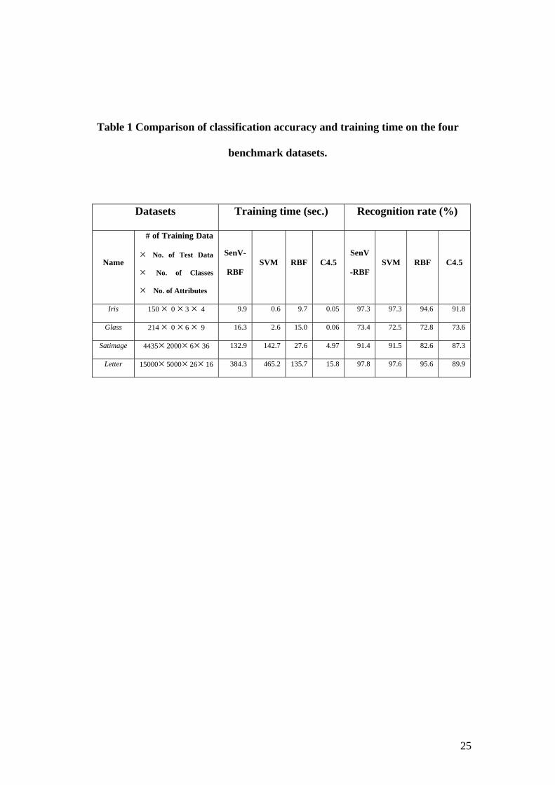
Table 1 Comparison of classification accuracy and training time on the four

benchmark datasets.

Datasets Training time (sec.) Recognition rate (%)

Name

# of Training Data

No. of Test Data

No. of Classes

No. of Attributes

×

×

×

SenV-

RBF SVM RBF C4.5

SenV

-RBF SVM RBF C4.5

Iris 150 × 0 × 3 × 4 9.9 0.6 9.7 0.05 97.3 97.3 94.6 91.8

Glass 214 × 0 × 6 × 9 16.3 2.6 15.0 0.06 73.4 72.5 72.8 73.6

Satimage 4435× 2000× 6× 36 132.9 142.7 27.6 4.97 91.4 91.5 82.6 87.3

Letter 15000× 5000× 26× 16 384.3 465.2 135.7 15.8 97.8 97.6 95.6 89.9

25

FIGURE LEGENDS

Figure 1. Illustration of the difference between sensitivity-based and conventional

RBF classifiers. The circles and balls represent data points of two classes respectively,

and RBF centers are indicated by extra circles. (a) Sensitivity-based RBF, centers

being the vectors sensitive to the classification. (b) Conventional RBF, centers being

the cluster centroids.

Figure 2. Classification of iris data with Sensitivity-based RBF. (a) Iris data points in

2-dimensional space of petal width and petal length. (2) The best classification

performance of 5-fold validation with =1.0. 2σ

Figure 3. Procedure for training RBF with the iris data in Figure 2.

26

TABLE LEGENDS

Table 1 Comparison of classification accuracy and training time on the four

benchmark datasets.

27