LAZY ENTREPRENEURS OR DOMINANT BANKS?

AN EMPIRICAL ANALYSIS OF THE MARKET

FOR SME LOANS IN THE UK

Otto Toivanen*

Email: toivanen@hkkk.fi

Economics Department, Helsinki School of Economics

PO Box 1210, 00101 Helsinki

Finland

and

Robert Cressy

Email: R.Cressy@city.ac.uk

City University Business School

London

United Kingdom

First version January 1998; this version December 2000

ABSTRACTAn encompassing model of a business loan contract with the bank is constructed toestablish the roles and relative importance of asymmetry of information, marketpower, borrower (entrepreneurial) effort and quality in explaining contract features.Special cases of the model include symmetric versus asymmetric information regimes,competition versus monopoly power, adverse selection versus moral hazard. Themodel is tested on a large SME database from a large UK bank. Results indicate thatthe model is a good description of the data; that the bank has considerable marketpower; and that there is moral hazard but no adverse selection in the market

Keywords: optimal loan contracts, adverse selection, moral hazard, symmetric information, monopoly,

empirical contract theory

JEL classification: D82, G21

* We would like to thank Ari Hyytinen, Leena Mörttinen, Hashem Pesaran and seminar participants

at the Helsinki microeconomics workshop and University of Cambridge for helpful comments. The

usual disclaimer applies.

1

I. INTRODUCTION

A considerable research effort has been directed to further our understanding

of the characteristics and determinants of loan contracts. One objective has been to

explain the stylized facts of such contracts: there is growing evidence that interest rate

margins, loan sizes and the level of collateral vary between seemingly similar customers

(see e.g. Cressy and Toivanen, 1998). But whilst during the last two decades, much

progress has been made in advancing our theoretical knowledge on how asymmetric

information affects optimal loan contracts (see Jaffee and Russell, 1976; Stiglitz and

Weiss, 1981; Bester, 1985; and Broecker, 1990). As is so often the case in economics,

theoretical work has predated the applied: very little has been achieved in terms of

structural empirical analysis. In addition to the general interest in what conditions

prevail when real world contracts are designed and how these conditions affect the

nature of the contracts, theoretical research would ideally need empirical results for

guidance.

The objective of this paper is therefore to contribute to the literature firstly, by

theoretically modeling optimal loan decisions under both symmetric and asymmetric

information when the loan contract has several (up to four) dimensions instead of the

usual two (interest rate and collateral); secondly, by allowing explicitly for imperfect

competition in the banking market (see Besanko and Thakor, 1987, for such a model);

and thirdly, by testing the model using loan level data from a representative UK bank.

We will use as a starting point of our analysis our recent paper by (Toivanen and

Cressy, 1998) where we built and estimated a model with a three dimensional (loan

size, collateral, and interest rate) loan contract, exogenous effort and competitive

banking markets that explained the stylized facts of credit markets under both

2

symmetric and asymmetric information (adverse selection). We found support for the

model’s predictions, and could not reject the null hypothesis of symmetric information.

Most of the existing theoretical literature adopts modeling structures that result

in a first best equilibrium where collateral plays no role. As we argued in (Toivanen

and Cressy, 1998, (CT), such models, although well suited for generating theoretical

insights, do not lend themselves to the task of generating testable hypotheses on the

informational structure of the credit market as they by assumption rule out one

possible structure, that of symmetric information. Likewise, the bulk of the emerging

empirical literature testing for a regime of asymmetric information (Puelz and Snow,

1994, Chiappori and Salanie, 1996, 1997, and Dionne et al., 1997) relies on reduced

form estimations. Though again well suited for the specific task of testing for an

asymmetric information regime, do not yield results on the wider issue of the

characteristics of the optimal contract. The existing empirical papers on loan contracts

(Berger and Udell, 1990 and 1992, Boot et al., 1991) also tend to focus on one or the

other dimension of the loan contract, and do not (explicitly) test the nature of the

informational regime. In addition, to the best of our knowledge, CT is the only paper

that explicitly derives an econometric test of the nature of the informational regime

from a theoretical model, and executes this test.

In the current paper we avoid the problems (from an empirical standpoint)

present in most of the theoretical banking literature by constructing a model that has a

role for collateral even under symmetric information. The intuition behind the result is

very straightforward: collateral represents an alternative means of payment. By

pledging collateral the customer raises the expected profit of the bank and can

therefore expect a lower interest rate in return. The customer then optimizes between

these alternative ways of paying the loan. Concentrating on banking and loan contracts

3

allows us to assume that both contracting parties are risk-neutral: we thereby avoid the

modeling problems presented by risk-aversion of one or the other party.

We use as a starting point the modeling framework of CT, but relax several of

the assumptions made there. Whereas they assumed competitive banking markets, we

allow for imperfect competition. This is done by modeling theoretically the two polar

cases of a monopolistic bank and a bank operating in fully competitive markets. We are

then able to show (in all but one version) of the model that only one parameter of the

loan contract (the interest rate) differs when the market structure assumption is

changed, and that one can therefore easily build an empirical model that encompasses

the two versions (monopoly, competitive markets) of the theoretical model. A

corollary of this is that our model of optimal loan contracts gives a theoretical

justification for the approach taken in several industrial organization-based studies on

banking competition (e.g. Spiller and Favaro, 1984, Suominen, 1994) where the

researchers have only modeled the interest rate, not the whole loan contract. One

novelty of our model is that it allows us to measure the degree of market power by

using data from a single firm (bank).

Whereas in CT we assumed that the type of the customer is exogenous, we

allow for the possibility that the type (i.e., the success probability) is an endogenous

variable. It turns out that this has distinct effects on the form of the optimal contract

both under symmetric and asymmetric information (moral hazard). The consensus view

in the literature in what is becoming known as ‘empirical contract theory’ seems to be

that one cannot distinguish moral hazard from adverse selection econometrically. One

contribution of this paper is to show that this indeed can be done. In fact, we show that

more than this is possible as we demonstrate a test for endogeneity of effort even

under symmetric information. Conditional on the model fitting the data, we are thus in

4

a position to test i) whether effort is endogenous or exogenous; ii) whether information

is symmetric or asymmetric; and iii) the degree of market power that the bank

possesses.

The next Section of the paper presents the basic model. We then solve in

Section III the monopoly and perfect competition versions of the model under the twin

assumptions of exogenous effort and symmetric information. After that, we relax the

assumption of symmetric information to allow for adverse selection, and again solve

the model under both competition regimes. We then proceed to analyze the case of

endogenous effort first under symmetric and then under asymmetric information (moral

hazard), and under both modes of competition, in Section IV. In Section V we discuss

how to build an empirical model that nests the different versions of the theoretical

model so as to allow the econometrician to test different assumptions. In the sixth

Section, we present the data and the estimation results. Section VII concludes and

summarizes.

II. THE BASIC MODEL

The basic structure of our model follows closely that adopted in CT. A risk

neutral entrepreneur maximizes expected profits by investing L either in a riskless

project with a rate of return r or in a risky project with gross return R(Xi, L) in success

states and 0 otherwise. R is an increasing, strictly concave and twice continuously

differentiable function of L, the size of the loan. Xi is a vector of observable,

quantitative entrepreneurial characteristics. Entrepreneurs have to finance their

projects entirely by bank loan.1 The success probability, denoted p X i i( , )θ , is a function

of Xi and a potentially endogenous and/or unobservable variable θ i called “effort”. We

assume that if exogenous, θ i is distributed according to some known density function

5

with support [ ]θ θ, . If endogenous, it is chosen from the interval [ [θ,∞ . The success

probability satisfies the following assumptions: p X i i( , )θ > 0 , p’>0, p’’<0 (where

primes denote derivatives w.r.t θ i ) and p X i( , )∞ <1 . These assumptions capture the

essential features of effort: that there is some lower limit of effort that results in a

positive probability of success; that the success probability is increasing in effort, but at

a decreasing rate; and that no level of effort guarantees success. The entrepreneur

negotiates the loan terms with a risk neutral, profit-maximizing bank. The loan terms

consist of loan size L, interest rate α , collateral C and possibly (under the assumptions

of endogenous effort and symmetric information) the level of effort θ . As in CT, we

assume that the cost of pledging collateral, f(Xi,C), is an increasing, twice

differentiable, strictly convex function of C. In order to allow that some firms find it

optimal to pledge zero collateral, it is assumed that f(0)>0 and f’(0)≤β , where a prime

again denotes a derivative,2 and β is a parameter of the model (see below). In case of

default, the firm’s value is zero in excess of whatever collateral was pledged: this

assumption (taken from CT) allows us to treat inside and outside collateral equally,

and conforms with the real-life definition of default.

The bank manager uses available quantitative information Xi to categorize3

entrepreneurs into different groups i, i=1,...,k, where the number of entrepreneurs in

group i is denoted Ni. The success probability p varies over entrepreneurs i, and within

each group with θ . Under symmetric information and exogenous effort the bank is

able to identify those customers within group i that have the same θ θ= j . The number

of customers within these subgroups is nij, which satisfies n Nij ij

J

==∑

1

. The bank hence

optimizes the loan for customers that exhibit similar characteristics, and is assumed to

6

be able to discriminate a) between customers with different observable and quantifiable

characteristics under all informational regimes and, b) between customers with

different observable, exogenous, qualitative characteristics under symmetric

information and exogenous effort. When effort is endogenous and information

symmetric, we assume that there exists some enforcement mechanism that enables the

bank to write the contract contingent on the effort level promised by the entrepreneur.

We do not specify in any more detail what form such a mechanism might take.

The entrepreneur’s objective function is then given by:

θθαθπ )(),()),(1(]),()[,( VifipiRipiF XVCXfXpLLXRXp −−−−= (1)

where V(XVi) is a cost of effort multiplier, and the cost of effort (in line with most of

the literature) is linear in the level of effort θ i . The vectors Xji, j∈{p,R,f,V}, may

contain common elements. This formulation allows for both exogenous effort (in

which case V(XVi)=0 for all i, and θ i is fixed) and endogenous effort. The objective

function of the bank is

π α β δB p L p C rL K= + − − − − =( )( )1 0 (2)

where r is the bank’s exogenously given cost of funds (deposit or world bond market

interest rate), K>0 is a fixed cost of writing the loan contract and β and δ are

parameters. We assume 0 1< ≤β and δ≥ 0 to hold. This set up allows for the

possibility that the bank does not recover the full market value of collateral in case of

default, and for the possibility that the bank has to incur some fixed cost in liquidating

the collateral.

Different combinations of assumptions on the symmetry of information, the

endogeneity of effort, and the level of competition in the loan market yield a total of

7

eight different regimes for which the model has to be solved. We will analyse this, and

state the results, in the following two Sections.

III. EXOGENOUS EFFORT

A. Symmetric Information

We start the analysis by assuming that the bank is able to discover the value of

θ i , which is here assumed to be exogenous. In other words, entrepreneurs in group Ni

vary, but the bank is able to find out the value of the qualitative characteristics of the

entrepreneurs, and can discriminate on the basis of that information. This means it can

offer loan contracts conditional on the value of θ i .

To solve for the optimal loan contract under the assumption of competitive

loan markets we solve the following program:

max , ,imize L CF

α π s.t. πB ≥ 0 (3)

It is easily established that the objective function is (strictly) concave and the constraint

(strictly) convex in their arguments,4 and hence the first order conditions of (3)

characterize the unique maximum. Based on these we can state the following

Proposition (see CT for a proof):5

PROPOSITION 1: a) Under the assumptions of i) competitive loan markets, ii)

exogenous effort and iii) symmetric information,

a) the optimal loan size is given (implicitly) by

R Lrp

' ( *) = (4)

b) the optimal interest rate is given by

α β δ*

*( * )

*= + − − −r

p pKL

pp

CL

1 1 (5)

c) and the optimal level of collateral (implicitly) by

8

f C'( *) = β (6)

where * denotes the equilibrium (optimal) value.

It follows from Proposition 1 that the level of collateral depends only on

exogenous variables; that entrepreneurs with a high probability of success get a larger

loan; and that they pay a lower interest rate than entrepreneurs with a low probability

of success if and only if ( * ) * *β δ αC L− < (or, equivalently, β δC rL K* *− < + ). Although

it is an empirical matter to establish whether the last claim holds, we will from now on

in the theoretical treatment assume this to be the case. When we change the

assumption of competitive loan markets to one of a monopoly bank, the program that

yields the optimal loan terms changes to

max , ;imize L CB

α π s.t. πF ≥ 0 (7)

Again, it can be shown that the first order conditions yield a unique maximum which

we characterize in the following Proposition:

PROPOSITION 2: a) Under the assumptions of i) a monopoly bank, ii) exogenous

effort and iii) symmetric information,

a) the optimal loan contract is otherwise determined by the same equations as in

Proposition 1, but the interest rate is given by equation

α*( *)

*( *)

*= − −R L

Lp

pf C

L1 (8)

b) One can empirically nest the monopoly bank and competitive loan market models

by estimating the following interest rate equation:

α γ γ β δ*

( *)*

( *)*

( )*

( * )*

= − −

+ − + − − −

R LL

pp

f CL

rp p

KL

pp

CL

11

1 1 (9)

where γ (satisfying [ ]γ∈ 01, ) is a measure of the monopoly power of the bank.

9

The intuition behind these results is that as the size of the loan determines the

total surplus, a monopoly bank has every incentive to give a loan that maximizes this.

The bank then uses the interest rate to capture the surplus left after the optimal amount

of collateral has been pledged. As the loan size (and therefore the surplus created by

the entrepreneur) is an increasing function of θ i , the interest rate is also an increasing

function of θ i . Proposition 2b follows simply from attaching weights to the interest

rate equations generated under the monopoly bank and competitive loan market

assumptions respectively. Under the current assumptions, we are thus able to infer

from the coefficient of the bank’s cost of funds (r) the level of market power enjoyed

by the bank.

B. Asymmetric Information (Adverse Selection)

We now change the assumption of symmetric information to allow for the

possibility that the bank is not able to find out the value of θ i . This means that within

each category Ni, the bank has to resort to incentive compatible contracts. For

simplicity, and in line with most of the literature (and CT), we assume that θ i can take

two values that satisfy θ θG B> (subscripts stand for “Good” and “Bad” borrowers

respectively). This assumption yields the following probabilities of success:

1 0> > >p pG B . We further assume that the bank knows the proportion χ of Good

borrowers in group Ni ( χN ni iG= )

If the loan market is competitive, the bank makes zero expected profits from

the loans it grants to entrepreneurs, and the program that the bank has to solve for

entrepreneur of type j (within group i) takes the form6

max , ;imize L C jF

α π s.t. πB ≥ 0 , π α π αjF

j j j jF

k k kL C L C( , , ) ( , , )≥ ,

10

π αjF

j j jL C( , , ) ≥ 0 j=G,B, j k≠

(10)

The new constraint is the familiar incentive compatibility constraint. As is common in

this type of models, the only constraint that binds (in addition to the bank’s zero profits

constraint) is the incentive compatibility constraint of the Bad borrower. We

summarize the results in Proposition 3 without proof (as the Proposition is identical in

content to that of Proposition 2 in CT):

PROPOSITION 3: Under the assumptions of i) competitive loan markets, ii)

exogenous effort and iii) asymmetric information, a separating equilibrium exists

where

a) the optimal loan contract of the Bad borrower is identical to that described in

Proposition 1;

b) A Good borrower’s optimal loan contract is otherwise similar to that described in

Proposition 1, but she pledges more collateral than a Bad borrower as determined by

equation (11):

f C f Cp

pR L L R L LG B

B

BG G G B B B( *) ( *) {[ ( *) * *] [ ( *) * *]}= +

−− − −

1α α (11)

We thus obtain the standard adverse selection result where the Good borrower

pledges more collateral than she would under symmetric information. This she does in

order to avoid dissembling by the Bad borrower. We next change the assumption of

competitive loan markets to that of a monopoly bank. The program that the bank

solves then takes the form

max ( ), ,imize G GB

B BBχπ χ π+ −1 s.t. π α π αj

Fj j j j

Fk k kL C L C( , , ) ( , , )≥ ,

π αjF

j j jL C( , , ) ≥ 0 j=G,B, j k≠

(12)

11

where the first subscript stands for the type of the entrepreneur, and the second for the

type of entrepreneur for whom the contract has been designed (i.e., πG GB

, gives the

profit of the bank from a contract that is designed for a Good borrower, and made

with an entrepreneur who is a Good borrower7). An important feature to be noted is

that under the current assumptions, it is the Good borrowers’ participation constraint

that is binding (if any). This is a consequence of characterizing the types via first order

stochastic dominance and hence holds e.g. in the models of Besanko and Thakor

(1987) and Wang and Williamson (1994; see Vauhkonen, 1997). In our model, it can

be shown that as long as the optimal contract is a separating one, the optimal loan sizes

are not affected by the other characteristics of the contract. The loan sizes in turn

determine in our model the surplus created by the contract, and from this fact and the

above feature of the model it follows that the bank can use the other dimensions of the

contract to capture this surplus without having to fear that the size of the surplus is

thereby affected. The bank would then ideally want to design contracts where the

participation constraints of both types bind: it can be shown that this is possible in our

model if and only if there are no non-pecuniary costs of bankrupCTy, i.e., f(0)=0. If

this condition does not hold, the bank has three options: it either designs a pooling

contract such that the participation constraint of one or the other type is binding (as in

Besanko and Thakor, 1987), or it designs a separating contract where the Bad

borrowers’ participation constraint is binding. Which of these three emerges as the

equilibrium contract depends on the (relative) expected surpluses created by the two

types, and the proportion of the types in the customer population. The results from

solving the program (12) are summarized in Proposition 4:

PROPOSITION 4: a) Under the assumptions of i) a monopoly bank, ii) exogenous

effort and iii) asymmetric information,

12

a) if f(0)=0 holds, the optimal loan sizes and interest rates of the Bad and the Good

borrower are identical to those described in Proposition 2, the optimal level of

collateral of the Good type is identical to that described in Proposition 2, and the

optimal collateral of the Bad type is zero

b) if f(0)=0 does not hold, the bank either

i) chooses a pooling contract that is identical to the contract of the Good or the Bad

borrower as described in Proposition 2 (which of these depends on the relative

profitability of the two contracts, and the proportion of Good and Bad types in the

customer population: see Appendix A for precise characterizations) or

ii) designs a separating contract.

The changes induced by a change in the assumption of the competitiveness of

the loan market are thus more dramatic under asymmetric information than symmetric

information when effort is exogenous. The result of Proposition 2b,i) resembles that of

Besanko and Thakor (1987) who in a model with exogenous loan size found that a

monopoly bank may set the interest rate such that Bad borrowers do not participate,

and the Good borrowers’ participation constraint is binding. Our results imply that

credit rationing in equilibrium is less likely than in the model of Besanko and Thakor:

the reason for the difference is that in our model, loan size is endogenous, and the cost

of collateral to the entrepreneur nonlinear. The above Proposition has crucial

repercussion to empirical testing of our model. These are summarized in the following

Corollary:

COROLLARY 1: If the bank is a monopolist, one can empirically distinguish an

exogenous effort, symmetric information version from the exogenous effort,

asymmetric information version of the model as long as the optimal contract under

13

asymmetric information is a separating contract. One can also test whether the

observed contracts are pooling or separating contracts.

The Corollary means that the test employed in CT to test for adverse selection

is not sensitive to the level of competition in the market as long as the optimal

monopoly contract under adverse selection is not a pooling contract.8

IV. ENDOGENOUS EFFORT

A. Symmetric information

In this Section we change the assumption of the exogeneity of θ i and assume

that it is endogenously chosen after the loan contract is signed. As discussed earlier,

we assume that under symmetric information the bank and the entrepreneur are able to

write a contract that is contingent on the level of effort exerted after the contract is

signed, and that there exists some mechanism that allows the bank to enforce the

agreed level of effort. This setup means that the loan contract has as its fourth

dimension the level of effort, and under the assumptions of symmetric information and

a competitive loan market the program to be solved changes from (3) to (14):

max , , ,imize L CF

α θπ s.t. πB ≥ 0 (14)

where p X i i( , )θ , is a function of θ i , which in turn is endogenously determined. Our

assumptions define a decreasing returns to scale technology with respect to producing

success with effort. The cost of effort is assumed linear as stated in (1). Solving (14)

yields Proposition 5:

PROPOSITION 5: Under the assumptions of i) competitive loan markets, ii)

symmetric information and iii) endogenous effort,

a) the optimal loan size, interest rate, and level of collateral are determined by

equations (4) - (6) as described in Proposition 1;

14

b) the following comparative statics w.r.t to the effort hold:

∂θ∂L

> 0 , ∂θ∂C

= 0 , ∂θ∂α

= 0 , ∂θ∂r

= 0 , ∂θ∂V

< 0 .

What emerges is that the equations determining the interest rate and loan size

are robust to the endogeneity of effort, as is the collateral equation (when compared to

the exogenous effort, symmetric information model). As effort is now part of the

contract, Proposition 5b defines the comparative statics of it with respect to other

variables of interest. It turns out that effort is an increasing function of loan size. None

of the other endogenous variables nor the bank’s cost of funds affects on effort. Not

surprisingly, increasing the cost of effort leads to a decrease in the level of it.

When changing the assumption from competitive loan markets to a monopoly

bank the program to be solved becomes

max , , ,imize L CB

α θπ s.t. πF ≥ 0 (15)

The results of solving (15) are summarized in Proposition 6:

PROPOSITION 6: Under the assumptions of i) monopoly bank, ii) symmetric

information and iii) endogenous effort,

a) the optimal loan size, interest rate, and collateral are determined as described in

Proposition 2;

b) the comparative statics w.r.t to the effort are as described in Proposition 5.

A monopolistic loan market shares the same features regardless of whether or

not effort is endogenous. The one departure from this rule is naturally the endogeneity

of effort: in this respect monopolistic and competitive loan markets are identical.

B. Asymmetric information (Moral Hazard)

We now relax the assumption that the bank observes the level of effort, and

that the parties can contract on it. Our assumptions on the technology and preferences

15

enable us to use the first-order approach (see e.g. Grossman and Hart, 1981,

Rogerson, 1985). In our model this means adding the constraint

[ ]p R L L f C V' ( ) ( )− + − ≥α 0 (16)

to the program which, if the banking market is competitive, now becomes

max , , ,imize L CF

α θπ s.t. πB ≥ 0 and (16). (17)

This results in Proposition 7:

PROPOSITION 7: a) Under the assumptions of i) competitive loan markets, ii)

asymmetric information and iii) endogenous effort,

a) the optimal loan size and interest rate are give by equation (4) and (5) as described

in Proposition 1;

b) the following comparative statics w.r.t to collateral hold:

∂∂CL

>< 0 when R' <

> α , ∂∂α

C > 0 , ∂∂Cr

= 0 , ∂∂

CV

> 0

c) the following comparative statics w.r.t to effort hold:

∂θ∂L

>< 0 when R' >

< α , ∂θ∂C

> 0 , ∂θ∂α

< 0 , ∂θ∂r

= 0 , ∂θ∂V

< 0

This time the changes compared to symmetric information are large: whereas

under symmetric information the level of collateral is a function of exogenous variables

only, under asymmetric information it is a function of loan size and interest rate in

addition to being a function of exogenous variables. Also should be noted that whereas

the exogenous variables work under symmetric information only through the cost of

collateral function f(.), they now affect the level of collateral in addition through the

probability of success and the cost of effort functions p(.) and V(.). When one

compares the comparative statics of effort, the most important (and anticipated)

difference is that under asymmetric information the level of collateral affects positively

on the level of effort, i.e., collateral can be (is) used to induce the entrepreneur to exert

16

effort. Under symmetric information there was no need for this. In addition, the level

of effort is a negative function of the interest rate. One should also note that the

collateral and effort comparative statics with respect to loan size are intertwined: when

the former is positive (negative), the latter has to be negative (positive).

With moral hazard, the level of collateral is identical for all customers within a

given group i. This level of collateral can be zero if the cost of effort is sufficiently

high. In such a case, the bank offers customers within a group a contract that is based

on their success probability when their effort level is θ . Empirically we observe

however that the level of collateral varies within groups (see Table 2 in CT). The

reason for this could be, e.g., that our vector of exogenous variables is not identical to

that used by the bank.

Changing the assumption on the competitiveness of the loan market to a

monopoly results now in the following program

max , , ,imize L CB

α θπ s.t. πF ≥ 0 and (16) (18)

and Proposition:

PROPOSITION 8: Under the assumptions of i) a monopoly bank, ii) asymmetric

information and iii) endogenous effort

a) the optimal loan size and the interest rate equation are determined as described in

Proposition 2;

b) the comparative statics w.r.t to collateral and the level the effort are identical to

those described in Proposition 7.

Once again, the only change that a shift in the competitiveness of the loan

market induces is a change in the interest rate equation. Otherwise the monopoly

17

bank’s optimal loan contract is determined by the same equations, and same

comparative statics, as that of a bank facing a competitive loan market.

V. THE ECONOMETRIC MODEL

A. The general model

The aim in this Section is to build an econometric model that nests the different

versions of the theoretical model explored in the two previous Sections. The equations

that determine the optimal loan contract under different assumptions are presented in

Table 1. As can be seen, the loan size equation is not affected by changes in the

assumptions about the symmetry of information, endogeneity of effort, or level of

competition. Although the equation stays the same, there is a difference between the

two effort assumptions in that when effort is endogenous, the loan size is a function of

one other endogenous variable (effort) whereas under exogenous effort it is

determined solely by exogenous variables. The interest rate equation depends on the

level of competition, but not on the symmetry of information or the endogeneity of

effort. As stated earlier, one can therefore easily build an estimation equation that nests

both the competitive loan market and the monopoly bank interest rate equations. The

level of collateral depends on whether information is symmetric or asymmetric, and

(under asymmetric information) on whether effort is endogenous or not. Lastly,

optimal effort (when endogenous), is affected by the assumption on the symmetry of

information, but not by the competitiveness of the loan market.

[TABLE 1: PREDICTIONS OF THE THEORY]

The above theoretical model suggests the following system of estimating

equations that nests all the eight different regimes that have been studied:

L* = g1(p*,r,XLi) (17)

α *= g2(L*,C*,p*,r,Xαi) (18)

18

p* = g3(α * ,L*,C*, r,Xpi) (19)

C* = g4(α * ,L*, p*,r,XCi) (20)

Where the Xji are vectors of exogenous variables. Our exogenous variables are

a vector (43) of industry dummies; a vector (6) of purpose of loan dummies; year and

quarter dummies indicating the timing of the loan; bank’s cost of funds (bank’s Prime

rate); GDP in the quarter of making the loan contract; duration of the loan and its

square; and interactions between these. We include industry dummies into all

equations; purpose of loan dummies into the loan size and collateral equations; year

dummies into the interest rate, collateral and success equations; quarter dummies into

all equations; GDP into all others but the loan size equation (it was insignificant in the

loan size equation and therefore dropped); and finally, purpose of loan dummy- and

duration of the loan-bank’s cost of fund interactions into the loan size equation. We

discuss the identification of the model in more detail below.

We will proxy effort by the probability of success as the comparative statics for

these two are (almost) identical.

B. The Estimation Strategy

Based on the above general empirical model (equations (17)-(20)), one can

then use the following estimation strategy to test the model and its different

assumptions:

1. The validity of the model can be tested using the loan size equation (17) and the

interest rate equation (18). Neither of them is affected by the endogeneity of effort

(apart from having to use instruments instead of observed values for some variables) or

the symmetry of information.

2. The level of bank market power: The interest rate equation will also produce a

measure of the market power of the bank as equation (8) tells that the coefficient of r

19

is ( )1 − γ /p, and γis a measure of the market power of the bank. If the loan size and

interest rate equations show that the model fits the data, we can proceed to test

3. The endogeneity of effort with equation (19). If effort is endogenous, it will be a

function of loan size; if exogenous, it will not be affected by any of the endogenous

variables. The comparative statics differ with changes in the symmetry of information,

and under asymmetric information effort is increasing in the level of collateral and

decreasing in the level of the interest rate, in addition to being a function of loan size.

The effort equation can therefore also be used to test whether there is

4a. Symmetric or asymmetric information if effort turns out to be endogenous.

Our comparative statics tell that collateral is also an increasing function of

effort if either effort is endogenous, or if effort is exogenous, but there is asymmetric

information. It is hence possible that we could detect a positive correlation between

these two variables in both the effort and the collateral equations. However, the timing

of events in the case of moral hazard suggests that the causality is one way, and more

specifically, that it runs from collateral to effort. The sequence of events in a standard

moral hazard model as ours is that at the time of contracting the parties agree on the

level of collateral, and the agent (the entrepreneur in our model) thereafter exerts the

amount of effort that is in her best interest, conditional on the terms of the contract.

The timing of events in the endogenous effort case suggests thus that the level of effort

in the collateral equation measures the existence of adverse selection.

Finally, no matter what the results from the effort equation, we can use the

collateral equation to test for

4b. (A)symmetry of information: if the effort estimation revealed that effort is

exogenous, the possibility of adverse selection still remains. In this case we include the

variable proxying success into the collateral equation as an exogenous variable to test

20

for adverse selection (as done in CT). Under symmetric information collateral is not a

function of the success probability, whereas under adverse selection the Good

borrowers are more likely to pledge collateral than Bad borrowers if the market is

competitive or the monopoly bank chooses separating contracts.

If, on the other hand, the effort estimation proves that effort is indeed

endogenous, the collateral equation will bring (further) light to the question of whether

or not loan contracts are made under symmetric or asymmetric information. Under

symmetric information collateral is a function of exogenous variables (those relating to

the type of the entrepreneur) only, whereas under asymmetric information (moral

hazard) it is a function of loan size (with a sign that is opposite to that in the effort

equation) and an increasing function of the interest rate.

C. Identification and Estimation

We identify each equation using exclusion restrictions. We instrument loan

size using purpose of loan – bank’s cost of fund interactions; the interest rate by the

bank’s cost of funds; and collateral mostly by purpose of loan dummies. In the interest

rate estimation we include the purpose of loan dummies into the second stage

equation, and therefore have to use a different instrument for collateral. We resort to

the same solution that we apply to the instrumenting of effort (our proxy for effort is

whether or not the loan succeeded): we use as an instrument the predicted value from

a semi-parametric (probit) estimation of the endogenous variable on a 3rd degree

polynomial of exogenous variables. The reason for using this approach is that linear

instruments turned out to work badly with effort. The reason for this is twofold: firstly,

only a relatively small proportion of all loans default; secondly, the relationship

between exogenous variables and success turned out to be highly nonlinear.

21

For each estimation equation, we report i) a Hausman test of the endogeneity

of each endogenous explanatory variable; ii) a Bound et al. (1998) test of instrument

validity, again for each endogenous variable separately;9 and iii) a Hausman test of

overidentification restrictions. We thus statistically test for the need of instrumenting

and the properness of our instruments both in the sense of them being sufficiently

correlated with the endogenous variable they instrument, and in the sense of not using

as instruments variables that ought to be included into the structural equation(s).

Two of our endogenous variables are discrete, suggesting the use of nonlinear

estimation methods. However, Angrist (1991) reports Monte Carlo evidence that when

the functional form is misspecified, a linear probability model (LPM) yields good

results especially when a dummy endogenous variable is used as an explanatory

variable. Both conditions apply to our data. It is unclear what the correct distributional

assumption is for the collateral and success equations (although CT report that their

collateral equation results are robust to changes in the functional form assumptions).

Both equations also contain a dummy endogenous variable. We therefore report LPM

estimates for both success and collateral. Also, we do not employ 3SLS to avoid

letting the misspesification of one equation affect the estimation of others.

VI. DATA AND EMPIRICAL RESULTS

A. Data

We employ the same data set as in CT; it consists of 2767 term loans granted to

small and medium sized enterprises by a single, representative UK bank between April

1st, 1987 and December 31st, 1990. We observe the industry of the entrepreneur, the

purpose of the loan (6 categories), its duration (in months), and the time of granting

the loan (by year and quarter). These are all treated as exogenous variables. In addition

we have collected information on the level of GDP in the quarter the loan was granted

22

(this was not used in CT). We also observe the bank’s prime rate in each quarter, and

use that to measure the bank’s cost of funds. The overall descriptive statistics are

presented in Table 2.

[TABLE 2: DESCRIPTIVE STATISTICS]

We treat the size of the loan and its interest rate as endogenous variables. Our

other two endogenous variables are discrete, namely whether or not collateral is part

of the loan contract, and whether or not the loan ‘succeeded’ (did not default fail by

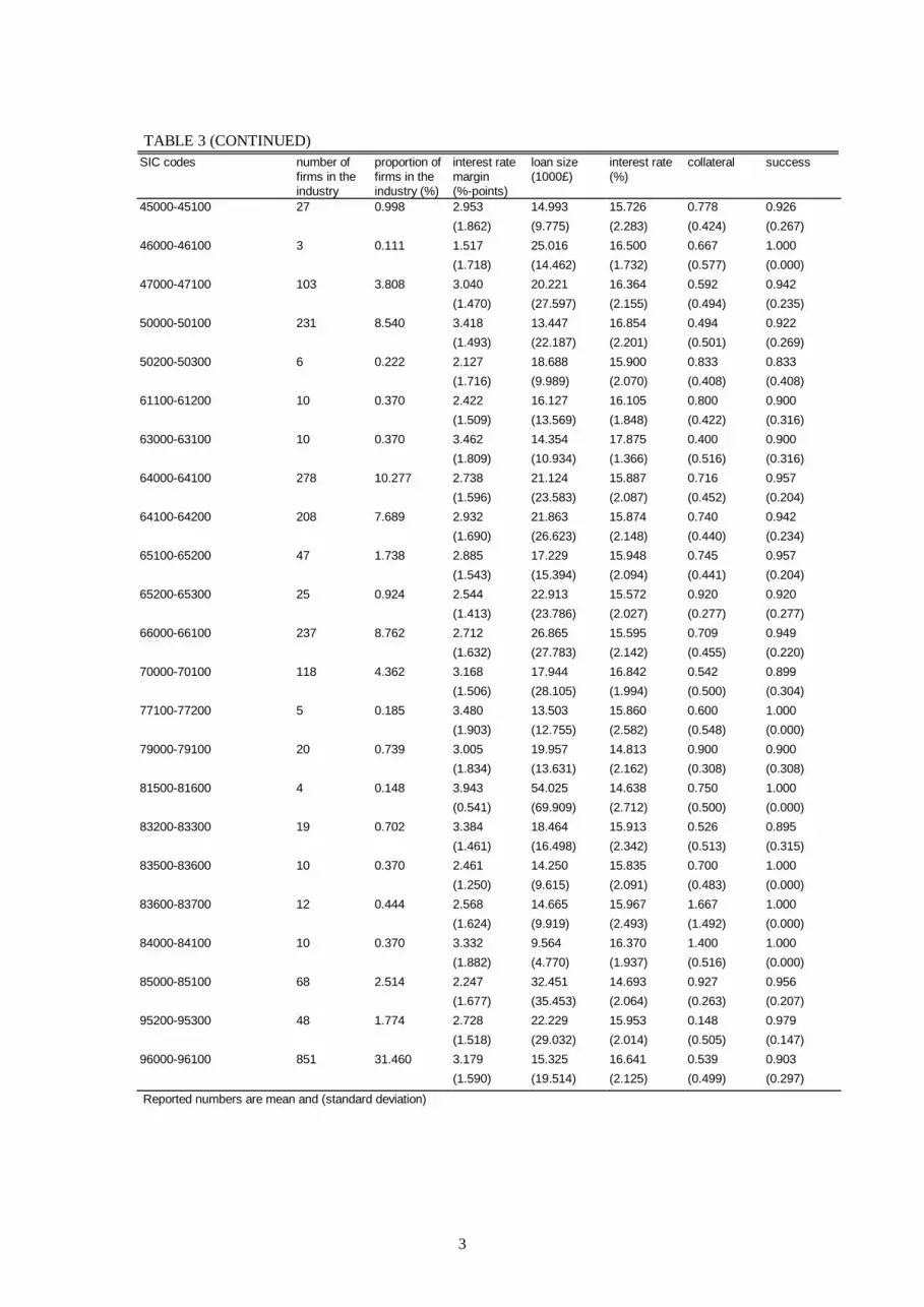
end of Quarter 1, 1993). Table 3 (reproduced from CT) gives the industry weighted

averages of the most important variables. The loans are small on average (£19 000)

and the interest rate margin is circa 3 percentage points. Over 60% of loans are

collateralized, and the average duration is 90 months. Some 8 per cent of the loans

defaulted (yielding a zero value for the success variable). As can be seen, there is large

variation (e.g. measured by the coefficient of variation) in each of the contract

variables. As CT discuss at length, this variation remains even when one controls for

the industry of the entrepreneur, and the purpose of the loan.10

[TABLE 3: INDUSTRY AVERAGES]

B. Empirical Results

Estimation results are presented in Table 4. In the lower half of the Table, we

report for each estimation the exogenous variables included into the (2nd stage)

equation, and the results of the tests discussed above. In the first column we report the

results of the loan size equation. As can be seen, the exogeneity of success is strongly

rejected.11 However, in line with our theoretical model, better firms (those with higher

effort) get a larger loan. This result leads us to reject the existence of a pooling

equilibrium (a possibility with a monopoly bank and adverse selection in our model;

and in other settings, too. See e.g. de Meza and Webb, 1989). In a pooling equilibrium

23

all types would get the same contract, and a positive and significant SUC coefficient

implies that Good applicants get a larger loan than Bad applicants. Loan size is a

decreasing function of bank’s cost of funds. Notice that the total effect of bank’s cost

of funds consists of the linear coefficient plus the coefficients of the purpose of loan-

bank’s cost of fund interactions, and the duration of the loan-purpose of the loan

interaction coefficient. The relationship between loan size and duration of the loan is

nonlinear, as already documented by CT. Our instruments for SUC pass both the

Hausman overidentification test and the Bound et al. test.

[TABLE 4: ESTIMATION RESULTS]

In Column 2, the interest rate is a negative function of loan size, though this is

only marginally significant. One should note that CT found, with this same data, and

treating loan size as endogenous, that the interest rate is an increasing function of loan

size. There are differences in the instruments used, and in that now we instrument SUC

in addition to loan size and collateral. This time, we cannot reject the Null that loan

size is exogenous to the interest rate (as suggested by our theoretical model). The

value of the Bound et al. test suggests that the result is genuine, and not due to weak

instruments. We therefore report in Column 3 the results of an estimation where loan

size is treated as exogenous. Now the coefficient of loan size is positive and

significant, in line with the CT results.

Bank’s cost of funds carries a positive coefficient of .154, although this is

significant at the 13% level only when we treat loan size as endogenous. When loan

size is treated as exogenous, the coefficient of bank’s cost of funds is significant at the

10% level with a slightly higher value of .198. Recall that 1/p times one minus the

coefficient on bank’s cost of funds is a measure of the market power of the bank.

Employing the point estimate from the equation where loan size is exogenous, and the

24

expected success rate in the sample, our estimate of bank market power is .794 on a

scale from 0 to one, 0 representing a monopoly.

One can make at least two kinds of comparisons to theoretical models. Firstly,

one could denote by 0 the price cost margin that a monopolist achieves in some

theoretical model, and calculate the number of firms needed to achieve the level of

competition suggested by our point estimate. Thus, to achieve a value .794, a linear

demand homogenous goods Cournot oligopoly should have (should act as

competitively as if there were) 1.5 firms. Alternatively, one could start from the

observation that in our model, the monopoly bank captures (almost) all the surplus.

One could therefore compare the industry surplus (total firm profits) to social surplus

generated by a given market structure in some theoretical model. In the linear demand

Cournot, a monopoly captures 2/3 of the social surplus, whereas our estimate suggests

that the bank captures 79%.

Turning to other variables, we find that the interest rate is a decreasing function

of both effort (success) and collateral, as predicted by our model. Duration affects the

interest rate in a nonlinear fashion, confirming the findings of CT. We conclude that

both the interest rate equation and the loan size equation suggest that our model is a

reasonable description of the data, and proceed to discuss the success (effort) and

collateral equations.

The success equation, reported in Column 4, is important both as a test of the

endogeneity of effort, and as a test of the (a)symmetry of information. Recall that if

effort is exogenous, success should not be a function of any of the other endogenous

variables; that if effort is endogenous and information symmetric, it should be a

function of loan size only (of the endogenous variables); and that if effort is

endogenous and there is asymmetric information (moral hazard), it should be a positive

25

function of collateral. Our specification passes the over-identification and instrument

validity tests. We find that success is not a function of loan size, and that we cannot

reject the Null that loan size is exogenous (treating it as exogenous did not change the

results, and we therefore only report the results from the estimation where loan size is

treated as endogenous). Interest rate obtains a coefficient of 5.150, which is significant

at the 13% level only. Therefore neither loan size nor the interest rate coefficients yield

support to the hypothesis that effort is endogenous. The collateral variable, in contrast,

obtains a positive coefficient that is significant at the 5% level. This results turned out

to be very robust to various experiments both with regard to instruments used (in the

reported equation, collateral is instrumented by the purpose of loan dummies vector),

and to exogenous variables included into the 2nd stage regression. The result leads us

to reject both the Null of exogenous effort, and the Null of symmetric information

(conditional on endogenous effort), and suggests that the data can be characterized by

moral hazard. Note that as almost 40% of loans are uncollateralized, this results

implies that these loans have no collateral because the cost of providing (more than the

minimum amount of) effort is too costly.

In the last column we report the results of the collateral estimation. This can be

used for verification of the moral hazard result of the success equation. If there is

moral hazard, collateral is a positive function of loan size, whereas otherwise it is not a

function of any of the other endogenous variables. We find a positive, statistically

significant coefficient for loan size, whereas the other two endogenous explanatory

variables (success, interest rate) carry imprecisely measured coefficients. We interpret

this as further evidence in favor of moral hazard. We fail to reject the Null of

exogeneity for both success and the interest rate. The insignificant coefficient of SUCC

means that, in line with CT, we cannot reject the Null of symmetric information against

26

the alternative of adverse selection (of course, the Null of symmetric information was

rejected in favor of moral hazard in the success estimation).

VII. CONCLUSIONS

Our objective in this paper was to build upon earlier theoretical and empirical

work in uncovering how loan contract terms are determined. We sought to generalize

an existing model so as to allow for different potential features of real life loan

contracts and contracting situations. In particular, we allowed the contract to have

several dimensions (up to four: loan size, interest rate, collateral and effort); and the

environment to vary in three ways (the degree of competition, the symmetry of

information, and the endogeneity of effort). This theoretical approach produced eight

versions of our basic model, each capable of a priori explaining the stylized facts of

credit markets. We then showed that one can build a general econometric model that

encompasses the different versions of the theoretical model, and devised a testing

strategy that starts from an empirical verification of the model, and continues with tests

of the different key assumptions that influence the determinants of loan contracts. Our

theoretical model shows how the empirical predictions of adverse selection and moral

hazard differ, and thereby allows us to test for the existence of one or the other. Most

previous empirical work on the (a)symmetry of information has tested reduced form

equations that do not allow the researcher to identify whether the form of asymmetric

information (if any) is adverse selection or moral hazard.

Our theoretical model showed that earlier results that suggest that monopoly

power of the bank may lead to pooling contracts and credit rationing are sensitive to

the specification of the model. In particular, making loan size endogenous and cost of

collateral nonlinear results in the possibility of separating contracts and no credit

rationing. Our model displays however the same feature as that of Besanko and

27

Thakor (1987) in that a monopoly bank facing adverse selection may not resort to

collateral as a signaling device and that there may be credit rationing in equilibrium. A

corollary of this is that the test used in our earlier paper to distinguish symmetric

information from adverse selection is not sensitive to the level of market power

possessed by the bank as long as we observe separating contracts.

We implemented this testing strategy using a data set explored in earlier work

(Toivanen and Cressy, 1998) and were careful to maintain comparability of our results

with those reported earlier. Our empirical results showed that the model explains the

data well and that thus our theoretical model seems to be an adequate description of

real world loan contracting; we were also able to show that the bank in question

possesses quite considerable market power in the market for small and medium sized

enterprise loans. Most importantly, in terms of contributing to the research program of

under what conditions are real world contracts designed, our results rejected the

hypotheses of symmetric information, exogenous effort and adverse selection in favor

of the hypotheses of endogenous effort and moral hazard.

Our results are important not only because they ex post justify the large

research effort of the last two decades that has been directed towards theoretical

modeling of (loan) contracts under asymmetric information (more specifically, moral

hazard: adverse selection was not found); but also because they (hopefully) can be

used as a starting point for further theoretical work. At the same time one should keep

in mind that although robust as such, our results are still comparable to one experiment

in natural sciences as we have used data from one bank operating in a particular

country, and our data is limited by the relatively short time period it covers. More

econometric work is called for before the profession can with any confidence claim to

28

know what kind of an environment is faced by agents designing real world (loan)

contracts.

29

REFERENCES

Angrist, Joshua D. , 1991, “ Instrumental variables estimation of average treatment effects in econometrics

and epidemiology”, 1991, NBER Technical working paper no. 115

Berger, Allen N. and Gregory F. Udell, 1990, Collateral, Loan Quality, and Bank Risk, Journal of Monetary

Economics, 25, 21-42

Berger, Allen N. and Gregory F. Udell, 1992, Some Evidence on the Empirical Significance of Credit

Rationing, Journal of Political Economy, 100, 1046-1077

Besanko, David and Thakor, Anjan V., 1987, Collateral and Rationing: Sorting Equilibria in Monopolistic

and Competitive Credit Markets, International Economic Review, 28, 671-689

Bester, Helmut, 1985, Screening vs. Rationing in Credit Markets with Imperfect Information,

American Economic Review, 75, 850-855

Boot Arnoud, Anjan V. Thakor and Gregory F. Udell, 1991, Secured Lending and Default Risk:

Equilibrium Analysis, Policy Implications and Empirical Results, The Economic Journal, 101

(May), 458-472

Chiappori, Pierre-André and Salanié, Bernard., 1996, “Asymmetric information in automobile insurance

markets: An empirical investigation”, 1996, mimeo, DELTA, Paris.

Chiappori, Pierre-André and Salanié, Bernard., 1997, “Empirical contract theory: The case of insurance

data”, European Economic Review, 1997, 41, 943-950.

Cressy Robert, and Toivanen, Otto 1998, Is There Adverse Selection in the Credit Market?, SME Centre

Working Paper, Warwick Business School, University of Warwick

de Meza, David and Webb, David., 1989, “The Role of Interest Rate taxes in Credit Markets with

Divisible Projects and Asymmetric Information”, Journal of Public Economics,

1989, 39, 33-44.

Dionne, George, Gourieroux, Christian, and Vanasse, Christian., 1997, “The informational content of

household decisions”, CREST wp. number 9701.

Jaffee, Dwight and Russell, Thomas., 1976, "Imperfect Information, Uncertainty and Credit Rationing",

Quarterly Journal of Economics, 90, 651-66

Leland, Hayne E. and Pyle, David H., 1977, Informational asymmetries, financial structure and financial

intermediation, Journal of Finance, 32, 371-387

30

Puelz, Robert and Snow, Arthur, 1994, Evidence on Adverse Selection: Equilibrium Signaling and

Cross-Subsidization in the Insurance Market, Journal of Political Economy, 102, 236-257

Stiglitz Joseph E. and Andrew Weiss, 1981, Credit Rationing in Markets with Imperfect Information,

American Economic Review 71, 3, 393-410

Table 1Determinants of Loan Characteristics

Exogenous Effort Endogenous EffortSymmetric Information Asymmetric Information Symmetric Information

Competition Monopoly Competition Monopoly Competition MonopolyLoan Size

R Lrp

' ( *) =

InterestRate α

β δ

**

( * )*

= +

− − −

rp p

KL

pp

CL

1

1

α*( *)

*( *)

*

=

− −

R LL

pp

f CL

1

α

β δ

**

( * )*

= +

− − −

rp p

KL

pp

CL

1

1

α*( *)

*( *)

*

=

− −

R LL

pp

f CL

1

α

β δ

** * **

*( * )

*

= +

− − −

rp p

KL

pp

CL

1

1

α*( *)

**

*( *)

*

=

− −

R LL

pp

f CL

1

α*

− 1

Collateralf C'( *) = β f C'( *) = β

Bad:f C'( *) = β

Good:f C f C

pp

R L L

R L L

G B

B

BG G G

B B B

( ) ( * )

{[ ( ) ]

[ ( *) * *]}

^

^ ^

= +

−−

− −1

α

α

Separatingcontracts:C*G>C*B

Poolingcontracts:C*G=C*B

f C'( *) = β f C'( *) = β

Effort exogenous [ ]p R L f C C V' ( *) ( *) *+ − − = 0

NOTES: Each of the cells contains the equation that either determines the equilibrium value of the variable in question, or the equation that is used to derive the comparative statisticsreported in the Propositions and in Table 2. For the adverse selection, monopoly bank case the loan size and interest rate equations are not strictly accurate as they depend on whether thecontracts are pooling or separating contracts. See Appendix A for details.

Table 2

DESCRIPTIVE STATISTICS

Variable Whole Sample

mean

(standard deviation)

Loan size (£000) 18.785

(22.406)

Interest rate (%) 15.964

(2.086)

Bank’s cost of funds (%) 13.020

(2.308)

Interest rate margin (%-points) 2.944

(1.556)

Default (%) 8.064

(24.491)

Collateral (%) 61.596

(46.581)

Duration (months) 90.640

(51.633)

2767 loans, 43 Industry dummies, 6 Purpose of loan dummies. Numbers are weighted using industry

dummies as weights (proportions of industries in the whole sample)

2

TABLE 3INDUSTRY LEVEL DESCRIPTIVE STATISTICS

SIC codes number offirms in theindustry

proportion offirms in theindustry (%)

interest ratemargin(%-points)

loan size(£000)

interest rate(%)

collateral(as proportionof all loans tothe industry)

success(as proportionof all loans tothe industry)

1000-1100 43 1.590 3.181 13.463 16.381 0.605 0.977(0.537) (12.937) (2.105) (0.495) (0.153)

1100-1200 30 1.109 2.236 14.539 16.213 0.767 0.967(1.603) (8.587) (2.173) (0.430) (0.183)

2000-2100 7 0.259 4.257 13.928 16.064 0.286 1.000(0.970) (16.291) (2.346) (0.488) (0.000)

3000-3100 4 0.148 3.365 5.320 16.413 0.500 1.000(2.138) (0.874) (2.105) (0.577) (0.000)

5600-5700 24 0.887 2.840 32.092 15.146 0.750 0.917(1.456) (33.944) (2.250) (0.442) (0.282)

5700-5800 9 0.333 3.902 9.249 17.089 0.556 0.889(1.515) (5.064) (2.391) (0.527) (0.333)

5900-6000 42 1.553 3.104 28.841 15.332 0.691 0.952(1.445) (44.790) (2.502) (0.468) (0.216)

21000-21100 2 0.074 2.500 25.931 16.000 1.000 1.000(1.414) (10.616) (0.707) (0.000) (0.000)

22000-22100 5 0.185 3.608 32.055 16.260 0.400 0.800(1.097) (57.285) (2.123) (0.548) (0.447)

24300-24400 4 0.148 4.745 4.449 18.875 0.000 1.000(0.441) (1.305) (0.433) (0.000) (0.000)

24700-24800 9 0.333 2.830 12.909 16.404 0.667 1.000(1.871) (11.628) (1.095) (0.500) (0.000)

25000-25100 3 0.111 1.167 29.162 15.500 0.334 1.000(1.155) (6.731) (0.000) (0.577) (0.000)

31000-31100 10 0.370 3.480 28.082 15.770 0.600 1.000(1.632) (34.151) (1.850) (0.516) (0.000)

32000-32100 27 0.998 3.243 18.265 15.994 0.482 0.926(1.582) (17.422) (2.413) (0.509) (0.267)

33000-33100 6 0.222 3.548 31.094 14.958 0.667 1.000(0.896) (45.890) (3.287) (0.516) (0.000)

34000-34100 22 0.813 2.802 16.745 16.200 0.591 0.955(1.725) (13.220) (2.015) (0.503) (0.213)

35000-35100 9 0.333 2.424 37.713 14.789 1.000 1.000(1.796) (34.372) (2.193) (0.000) (0.000)

36100-36200 4 0.148 2.130 21.554 13.950 0.750 1.000(1.853) (11.095) (1.836) (0.500) (0.000)

37000-37100 44 1.627 2.368 17.197 16.135 0.750 0.955(1.595) (14.790) (2.079) (0.438) (0.211)

41000-41100 29 1.072 2.330 22.193 16.286 0.655 0.897(1.400) (26.849) (1.892) (0.484) (0.310)

42500-42600 3 0.111 2.500 5.915 17.500 0.333 1.000(1.732) (3.856) (1.732) (0.577) (0.000)

43000-43100 19 0.702 2.744 23.789 16.261 0.684 0.790(1.780) (20.326) (1.887) (0.478) (0.419)

3

TABLE 3 (CONTINUED)SIC codes number of

firms in theindustry

proportion offirms in theindustry (%)

interest ratemargin(%-points)

loan size(1000£)

interest rate(%)

collateral success

45000-45100 27 0.998 2.953 14.993 15.726 0.778 0.926(1.862) (9.775) (2.283) (0.424) (0.267)

46000-46100 3 0.111 1.517 25.016 16.500 0.667 1.000(1.718) (14.462) (1.732) (0.577) (0.000)

47000-47100 103 3.808 3.040 20.221 16.364 0.592 0.942(1.470) (27.597) (2.155) (0.494) (0.235)

50000-50100 231 8.540 3.418 13.447 16.854 0.494 0.922(1.493) (22.187) (2.201) (0.501) (0.269)

50200-50300 6 0.222 2.127 18.688 15.900 0.833 0.833(1.716) (9.989) (2.070) (0.408) (0.408)

61100-61200 10 0.370 2.422 16.127 16.105 0.800 0.900(1.509) (13.569) (1.848) (0.422) (0.316)

63000-63100 10 0.370 3.462 14.354 17.875 0.400 0.900(1.809) (10.934) (1.366) (0.516) (0.316)

64000-64100 278 10.277 2.738 21.124 15.887 0.716 0.957(1.596) (23.583) (2.087) (0.452) (0.204)

64100-64200 208 7.689 2.932 21.863 15.874 0.740 0.942(1.690) (26.623) (2.148) (0.440) (0.234)

65100-65200 47 1.738 2.885 17.229 15.948 0.745 0.957(1.543) (15.394) (2.094) (0.441) (0.204)

65200-65300 25 0.924 2.544 22.913 15.572 0.920 0.920(1.413) (23.786) (2.027) (0.277) (0.277)

66000-66100 237 8.762 2.712 26.865 15.595 0.709 0.949(1.632) (27.783) (2.142) (0.455) (0.220)

70000-70100 118 4.362 3.168 17.944 16.842 0.542 0.899(1.506) (28.105) (1.994) (0.500) (0.304)

77100-77200 5 0.185 3.480 13.503 15.860 0.600 1.000(1.903) (12.755) (2.582) (0.548) (0.000)

79000-79100 20 0.739 3.005 19.957 14.813 0.900 0.900(1.834) (13.631) (2.162) (0.308) (0.308)

81500-81600 4 0.148 3.943 54.025 14.638 0.750 1.000(0.541) (69.909) (2.712) (0.500) (0.000)

83200-83300 19 0.702 3.384 18.464 15.913 0.526 0.895(1.461) (16.498) (2.342) (0.513) (0.315)

83500-83600 10 0.370 2.461 14.250 15.835 0.700 1.000(1.250) (9.615) (2.091) (0.483) (0.000)

83600-83700 12 0.444 2.568 14.665 15.967 1.667 1.000(1.624) (9.919) (2.493) (1.492) (0.000)

84000-84100 10 0.370 3.332 9.564 16.370 1.400 1.000(1.882) (4.770) (1.937) (0.516) (0.000)

85000-85100 68 2.514 2.247 32.451 14.693 0.927 0.956(1.677) (35.453) (2.064) (0.263) (0.207)

95200-95300 48 1.774 2.728 22.229 15.953 0.148 0.979(1.518) (29.032) (2.014) (0.505) (0.147)

96000-96100 851 31.460 3.179 15.325 16.641 0.539 0.903(1.590) (19.514) (2.125) (0.499) (0.297)

Reported numbers are mean and (standard deviation)

4

Table 4ESTIMATION RESULTS

Loan size Interest rate Interest rate Success CollateralConst. 65.394

(89.895)1.047***(.052)

1.070***(.065)

-3.563(3.734)

-2.705:(6.183)

AM - -.0003*(.0002)

.043*** a

(.018).0006(.0043)

0.011**(.004)

INTRATE - - - 5.150(3.488)

3.588(5.922)

BRATE -106.010(75.503)

.154(.102)

.198*(.123)

- -

SUC 51.855***(9.294)

-.028***(.008)

-.044***(.010)

- .398(.497)

COLL - -.040***(.006)

-.055***(.003)

.391**(.174)

-

DUR 1.705***(.679)

.120*** a

(.366)-.133*** a

(.047)-.0026(.0008)***

.008***(.003)

DUR2 -.001***(.0002)

-.312*** b

(.121)-.285*** b

(.153).0069***(.0027)

-.195*** a

(.075)P1B 4.631

(20.705)- - - -

P2B 157.26**(68.489)

- - - -

P3B -95.938(119.870)

- - - -

P4B 172.48(161.81)

- - - -

P5B -4.922**(1.767)

- - - -

P6B 175.80**(84.494)

- - - -

DURB -1.188**(.581)

- - - -

Nobs. 2767 2767 2767 2767 2767Industrydummies

Yes Yes Yes Yes Yes

Purpose of loandummies

Yes No No No Yes

Quarterdummies

Yes Yes Yes Yes Yes

Year dummies No Yes Yes Yes YesGDP No Yes Yes Yes YesEAM - .9929 - .8020 .0676EINTRATE - - - .0399 .1293ESUC .0000 .0029 .0029 - .4187ESEC - .0000 .0000 .0386 -BAM - .0557 - .0000 .0003BINTRATE - - - .0000 .0050BSUC .0000 .0000 .0000 - .0000BSEC - .0000 .0000 .0925 -OI 1.000 .5292 1.000 .3026 .1689Notes: reported numbers are coefficient and heteroskedasticity robust (standard error).PiB, i=1,… ,6 are purpose of loan dummy-bank’s cost of fund interactions. DURB is the interaction betweenduration of the loan and bank’s cost of funds.Ei = Hausman test of endogeneity of variable i. Reported number is p-value.Bi = Bound et al. test of instrument validity for variable i. Reported number is p-value.OI = Hausman overidentification test. Reported number is p-value.*** = significant at the 1% level** = significant at the 5% level* = significant at the 10% levela = coefficients and standard errors multiplied by 1000.b = coefficients and standard errors multiplied by 10 000.

5

FOOTNOTES:

1 We assume that they have either zero wealth or assets tied to idiosyncratically valued and/or

illiquid assets. Adding the possibility that the entrepreneur invests some of her wealth into the project

does not materially change the results.

2 Our assumptions allow for the possibility that an entrepreneur i) in case of bankrupCTy

incurs costs on and above the loss of collateral (e.g. the loss of reputation) and ii) pledges collateral

that is worth more to her than to the bank, a case which casual observations seem to support. See CT

(footnote 14) for more discussion.

3 Snow and Crocker (1986) and Bond and Crocker (1990) analyze theoretically the welfare

effects of exogenous and endogenous categorization respectively in an insurance market model.

4 Strictly speaking, a participation constraint for the entrepreneur should be added to (3). We

will assume throughout that the participation constraints are satisfied under the assumptions of

competitive loan markets, and the constraint is hence superfluous in (3). If the constraint was binding

under the assumptions of competitive loan markets and symmetric information, analyzing the cases of

asymmetric information and a monopoly bank would not be necessary anymore as either the

participation constraint would be violated under these assumptions, or the results would be identical to

those obtained under the current assumptions. The participation constraints will play an important

role when analyzing the monopoly bank case.

5 Unless otherwise stated, the proofs of the Propositions are given in Appendix A.

6 We assume that there is no cross-subsidization.

7 This can only be done because the incentive compatibility constraint ensures truth-telling bythe Bad borrower.

8 CT reject in their empirical Section the Null hypothesis of pooling contracts. Hence their

result of no adverse selection is not caused by their assumption of a competitive loan market. We will

execute the same test in this paper.

9 This necessitates us to make choices as to which instruments are purported to instrument

each endogenous variable.

10 See CT for a more in depth discussion of the data.

6

11 This is in contrast to CT, who executed the same test and failed to reject the Null of

exogeneity. The reasons for the difference are twofold. Firstly, we employ a more powerful instrument

for SUCC; secondly, the equations differ slightly in what exogenous variables are included.