applying frontier cells based exploration and lazy theta* path

JINT manuscript No.(will be inserted by the editor)

Applying frontier cells based exploration and Lazy Theta*path planning over single grid-based world representation forautonomous inspection of large 3D structures with an UAS*

Margarida Faria, Ivan Maza and Antidio Viguria

Received: date / Accepted: date

Abstract Aerial robots are a promising platform to perform autonomous inspection of in-frastructures. For this application, the world is a large and unknown space, requiring lightdata structures to store its representation while performing autonomous exploration and pathplanning for obstacle avoidance. In this paper, we combine frontier cells based explorationwith the Lazy Theta* path planning algorithm over the same light sparse grid - the octreeimplementation of octomap. Test-driven development has been adopted for the software im-plementation and the subsequent automated testing process. These tests provided insightinto the amount of iterations needed to generate a path with different voxel configurations.The results for synthetic and real datasets are analyzed having as baseline a regular gridwith the same resolution as the maximum resolution of the octree. The number of iterationsneeded to find frontier cells for exploration was smaller in all cases by, at least, one order ofmagnitude. For the Lazy Theta* algorithm there was a reduction in the number of iterationsneeded to find the solution in 75% of the cases. These reductions can be explained both bythe existent grouping of regions with the same status and by the ability to confine inspectionto the known voxels of the octree.

Keywords Structure Inspection · UAS Applications · Path Planning · AutonomousExploration

1 Introduction

The increasing need of UAS usage for remote off-shore monitoring activities has raised dif-ferent challenges. The European Strategy for Marine and Maritime Research states the need

*The first author has been funded by the European Unions Horizon 2020 research and innovation programmeunder the Marie Sklodowska-Curie grant agreement No 64215 and the other two authors received fundingfrom the MULTIDRONE (H2020-ICT-731667) and AEROARMS (H2020-ICT-644271) European projects

Margarida Faria E-mail: [email protected] and Antidio Viguria E-mail: [email protected] for Advanced Aerospace Technologies, Calle Wilbur y Orville Wright, 19, 41300 La Rinconada,Sevilla, Spain

Ivan Maza E-mail: [email protected] the Robotics, Vision and Control Group, University of Seville, Avda. de los Descubrimientos s/n, 41092,Sevilla, Spain

2 Margarida Faria, Ivan Maza and Antidio Viguria

to protect the vulnerable natural environment and marine resources sustainably. The use ofUAS provides increased endurance and flexibility while reducing environmental impact, therisk for human operators and the total cost of operations. The work in this paper has been de-veloped in the framework of the MarineUAS 1 initiative, a European Union funded doctoralprogram which strategically strengthens research training on Unmanned Aerial Systems forMarine and Coastal Monitoring.

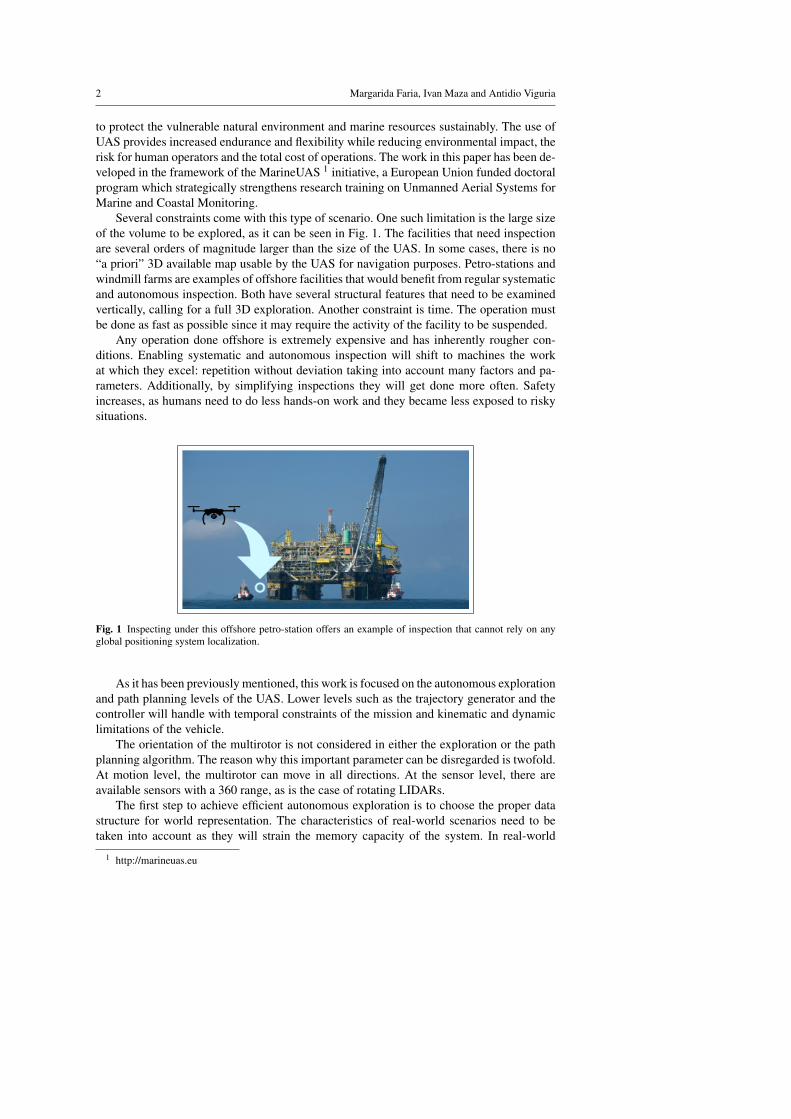
Several constraints come with this type of scenario. One such limitation is the large sizeof the volume to be explored, as it can be seen in Fig. 1. The facilities that need inspectionare several orders of magnitude larger than the size of the UAS. In some cases, there is no“a priori” 3D available map usable by the UAS for navigation purposes. Petro-stations andwindmill farms are examples of offshore facilities that would benefit from regular systematicand autonomous inspection. Both have several structural features that need to be examinedvertically, calling for a full 3D exploration. Another constraint is time. The operation mustbe done as fast as possible since it may require the activity of the facility to be suspended.

Any operation done offshore is extremely expensive and has inherently rougher con-ditions. Enabling systematic and autonomous inspection will shift to machines the workat which they excel: repetition without deviation taking into account many factors and pa-rameters. Additionally, by simplifying inspections they will get done more often. Safetyincreases, as humans need to do less hands-on work and they became less exposed to riskysituations.

Fig. 1 Inspecting under this offshore petro-station offers an example of inspection that cannot rely on anyglobal positioning system localization.

As it has been previously mentioned, this work is focused on the autonomous explorationand path planning levels of the UAS. Lower levels such as the trajectory generator and thecontroller will handle with temporal constraints of the mission and kinematic and dynamiclimitations of the vehicle.

The orientation of the multirotor is not considered in either the exploration or the pathplanning algorithm. The reason why this important parameter can be disregarded is twofold.At motion level, the multirotor can move in all directions. At the sensor level, there areavailable sensors with a 360 range, as is the case of rotating LIDARs.

The first step to achieve efficient autonomous exploration is to choose the proper datastructure for world representation. The characteristics of real-world scenarios need to betaken into account as they will strain the memory capacity of the system. In real-world

1 http://marineuas.eu

Title Suppressed Due to Excessive Length 3

environments, the free space is usually grouped. Particularly in offshore structures, it is alsolikely to occupy most of the area. Also, the occupied space is often clustered, like the pillarsin an offshore platform, the windmill’s tower or its blades.

The characteristics of the features used for autonomous navigation should also be takeninto account. The driving goal of the UAS is to explore a given volume. Many options areavailable, but this work is focused on the classical and widely used frontier explorationapproach.

This exploration has the advantage of simplicity. By first integrating a simple algorithmwe create the possibility of checking its limitations for the particular application experimen-tally. Another advantage is that allows to keep down the computational load. A frontier cellis a location in the world representation map that is explored and unoccupied but has unex-plored space in its vicinity. These places are of particular interest as they yield the highestinformation gain.

Due both to the focus on low memory requirements and information organization, thedata structure selected will be the octree implementation done in the octomap [1] framework.

Techniques from software development will be adopted in the implementation to enablereproducibility. Namely test-driven development, supported by automated unit tests. In thismethodology, a unit test is first designed to assert the implementation of a feature. Thenthe feature is developed until the test is passed, at which point another unit test is designedfor another feature. This process continues iteratively until the full desired functionality isachieved. To verify the result of the algorithm under different initial conditions this formof testing will be used whenever possible. Furthermore, both algorithms will be applied tosimulated and experimental data.

This paper extends previous work presented in [2]. The novelty of this work relies onthe implementation of both the frontier cells exploration algorithm and the Lazy Theta*path planning algorithm over the same data structure for the representation of the 3D en-vironment. This data structure can scale to large scenarios. No local reduction to a regulargrid will be used at any point. The frontier cell algorithm was chosen for its simplicity. Thegroup of suitable path planning algorithms is reduced as this is a single query problem. Bychoosing an Any-angle path planning algorithm the need of post-processing is significantlydecreased, and in particular, Lazy Theta* is further optimized to reduce the number of lineof sight checks. In addition, this algorithm has been applied successfully in competitionswith autonomous multirotors [3].

The paper is organized as follows. Section 2 reviews related work in data structures forenvironment representation, exploration algorithms and path planning techniques. Section 3reports relevant aspects for finding frontier cells on the different data structures under anal-ysis. Section 4 describes the challenges and solutions adopted for the implementation, amodification of the baseline algorithm as well as the methods chosen to develop the code.In Sect. 5, the results obtained both with simulated and experimental data with each of thealgorithms are detailed. Finally, section 6 closes the paper with the conclusions and futurework.

2 Related Work

This section presents the data structures considered for storing the representation of theworld, state of the art algorithms for autonomous exploration and path planning techniqueswith particular attention to the supporting data structures.

still call it grid based after adding visibility graphs and kd trees?


2.1 Efficient data structures for world representation

In this paper, several data structures have been analyzed, with a greater focus on those whichare readily available as off the shelf libraries. The amount of data translated into point cloudsfrom most sensors is exceptionally high. Thus, it is crucial to identify data structures thatmore than just compress data, also arrange information in an useful and efficient manner.One technique to organize the information is to create meshes. A popular algorithm is theDelaunay triangulation. Both PCL and CGAL [4] libraries provide implementations thatconstruct meshes from the points clouds. This technique has the drawback of being depen-dent on the order the points are analyzed, introducing one additional source of variability.[5] overcomes this issue by creating a mesh for the visibility graph, around found obstacles,showing the computational time advantages of constructing visibility graphs for multiplequery cases. Visibility graphs simplify the task of searching for neighbors by quantifyingthe relationship between samples according to the adopted metric. In [6], a software pack-age for their generation is presented. This package brings into Matlab a tool to computeobstacle avoiding paths in a known world.

Another option is to discretize the world into spaces of the same dimension. Creating aregular grid can be done even without a dedicated library, in less elaborated cases. In thesesimple cases, random access can have a complexity of O(1). Any information can be storedper cell, although with more information comes increased memory usage.

To make the search more efficient, trees (with all their multitude of implementationsand variations) are another option. The kd-trees are one option for the representation of theworld [7]. In this representation, the separation of space is a reflexion of the topology ofthe existing objects resulting in a tree that precisely matches it. The PCL library offers oneimplementation integrating the FLANN library, where the kd-tree is used [8].

The octree is a flatter tree compared to the binary kd-tree due to its eight children. Thetopology is less closely reflected but has the advantage of a smaller hierarchical traversalof nodes when finding nodes in the neighborhood. Two notable implementations of thisstructure are available: the octomap library [9] and the PCL library. The latter offers severalstructures; this paper is focused on OctreePointCloudOccupancy [10]. Both offer randomaccess with O(1) complexity and multiresolution queries. However, they differ in importantdetails. The PCL library has a significant focus on the compression needed for streaming,while the octomap library targets navigation and exploration. In the PCL library, new mea-surements are added by summing points whereas the octomap library integrates them in aprobabilistic manner. The concept of unknown space is also slightly different in each imple-mentation. In the PCL library, space is either occupied or free. In the octomap library, onlylocations with information are created thus implicitly encoding unknown space. Both PCLand octomap libraries concern themselves with efficiency: the former focuses on read/writeefficiency and for this reason, goes so far as to include a double buffered version of the struc-ture. In the latter, the focus lies on memory efficiency with (almost) lossless compressionregarding occupancy. For this reason, each node stores only the occupancy probability andone child pointer - forfeiting voxel size, coordinates, and the full children array.

2.2 Exploration

The concept of a frontier and a frontier cell repeatedly appears in the literature with the samebasic idea. Frontier locations or cells are points in the world representations that satisfy twoconditions: they are in free space and are connected to unexplored space. Due to the focus


on the underlying data structures and world representation, each work will be analyzed withthese aspects in mind, keeping in sight how to identify the locations that yield the higherinformation gain.

Unmanned Ground Vehicles (UGVs) are particularly well suited to reduce the searchspace to 2D, due to their motion constraints. Many applications use probabilistic occupancygrids to tackle the task of exploring unknown (or partially unknown) spaces in a 2D searchspace. Reference [11] explains the concept of frontier cells over a regular grid in the contextof probabilistic occupancy. This concept is not new, it was presented in [12], but due toits simplicity, it is still in use nowadays. In [13] an UGV is directed to the nearest frontierregion, leaving the task of path planning to a lower level of the architecture with purelyreactive obstacle avoidance. In [14], an UGV also travels to the nearest unexplored cell butcreates roadmaps, i.e., Voronoi diagrams generated from the occupancy grid.

Many approaches [13,15–17] encode the status of the cells as free, unknown and oc-cupied either explicitly or by probability thresholds. Here each cell encodes a somewhatdifferent approach to status: free, warning, travel and far. In [18] this approach is extendedto multiple vehicles. Each frontier cell is scored according to a heuristic combination ofoccupancy probability and distance traveled. With this combination, the path planning prob-lem is solved with the steepest descent of the heuristic function. In [19] the concept of afrontier is combined with a topological map: these edges are calculated as equidistant pointsto obstacles, the robot then travels this edges marking them as explored. The process con-tinues for as long as there are unexplored edges. Reference [13] is an example of applyingthis approach to UAS by setting a safe altitude. The frontier cells found at this altitude arethen clustered into labeled regions, disregarding the small and inaccessible frontiers. Theremaining ones are considered as goals for the UAS, finding the next goal by applying avector field histogram.

In 3D space, there are some applications of probabilistic occupancy grids to solve thenext best view problem for robotic arms. In [17], to distinguish between unknown and un-occupied cells a ray casting algorithm is used to extrapolate free regions from the sensorlocation and occupied points. Holes in sensor measurements are extrapolated with MarkovRandom Fields. The frontier cells are scored integrating all this information into the gain tobe later selected as best view. One example where the mission objectives are heavily takeninto account is [16]. From the probabilistic grid, a mesh is created as a tool to find voidregions. Unknown cells are set at the center of ellipsoids, which expand while maintaining aminimum fitting quality. The ellipsoids are then combined with frontiers and scored accord-ing to neighboring voids. The heuristic function maximizes the information gain taking intoaccount the priority each region has for the mission. Knowledge about the area critical forobstacle avoidance has the highest priority, followed by the regions affected by the robot’stools.

Another structure used for 3D space is the octree, being its multi-resolution quality oneof its defining characteristics. In [15] the list of frontier cells is compressed as clusters withan union-finding algorithm. The unknown spaces are handled as macro-regions through el-lipsoid expansion. Finally, the clusters are combined with the ellipsoids to score frontiersaccording to unknown region dimension. Another paper using the octree as its underlyingstructure is [20]. However, the configuration space is searched employing a Rapidly Ex-ploring Random Tree, grown iteratively through safe configurations in the direction of thefrontier. In [21] the information of the known space is stored in a map structure similar to anelevation map, although for other purposes the associated point cloud is stored in differentdata structures. The search for areas with higher information gain is done through samplegeneration, to address the issue of search space explosion in 3D. From a sample of known


points of the environment, other points are generated and added to the pool. The model dy-namics of the expansion of the molecules of a perfect gas is used to generate these points.Then, change rate between particle expansions is evaluated to find frontiers in regions.

2.3 Path Planning

In the field of motion planning, the problem of path planning has been extensively studied.Reference [7] presents different techniques within sampling-based motion planning, updat-ing the motion planning algorithms presented in classical references such as [22,23].

To plan paths in 3D environments is complex and different methods have been proposedfor online and offline planning. After considering the resource limitations (both regardingtime and of computation) of an aerial robot, two approaches stand out as most frequentlyused: deterministic and non-deterministic, each one encompassing several methods. Whengenerating paths with the deterministic approach is common to use probability as well assampling. With the non-deterministic approach, both heuristic and graph-based methods arefrequent.

The cost of building a fully connected graph is a good trade-off when solving a multi-query problem. One option when in a single query problem is to update the connectivity ofthe graphs taking into account the changes in the environment. In [24] this implementationis made dramatically reducing the cost of rebuilding the visibility graph. Another general-ization of the visibility graphs from 2D to 3D is found in [25]. In this implementation, thevisibility graph is composed of one obstacle graph and two supporting graphs. This approachrelies on a world that is previously known.

Sampling-based algorithms like Rapidly-Exploring Random Trees (RRT) [26], [27]and Probabilistic Rad Maps (PRM) [28], are specifically designed to handle non-holonomicconstraints (e.g., wheeled robots), high degrees of freedom and large spaces that require be-ing rapidly and uniformly explored. A typical use case is a big manufacturing plant. Severalvariations of the RRT have been proposed. RRT* [29] produces very optimal paths at theexpense of real-time rates. RRT-Connect [30] resolves the time issue, achieving faster solu-tions but generating longer paths. In [31], different probabilistic methods are used to solvethe motion planning problem with UAVs. A continuous-time trajectory optimization methodis used for real-time collision avoidance on multirotor UAVs.

The heuristic algorithms are specially designed to obtain the shortest path, exploringdirectly from the initial state to the target state. Examples are A* [32], Theta* [33] andD* [34]. These restrict the explored areas and get a runtime that is highly configurable anddependent on the number of variables and their resolution. The usual drawback imposedby discrete search techniques is that paths are formed by grid edges, so they are often notthe shortest path in the continuous space. Fortunately, this issue was solved by the any-angle path planning Theta* and its Lazy Theta* variation [35], which also optimizes thecomputational load of the algorithm. One example of the application of a graph algorithmto a 3D search space is [36]. Here a simulated micro-UAS vehicle goes from start to goalusing an AD* search algorithm for replanning. The underlying world representation is a3D occupancy grid that is sampled where the samples are arranged as a multi-dimensionallattice.

Other solutions to generate 3D paths for aerial vehicles have been presented taking com-pletely different approaches [37]. There are some examples of bio-inspired algorithms usingneural networks [38], evolutionary algorithms [39] [40]. Others combine several algo-rithms in one architecture to benefit from the strengths of each one [41], [42], [43].


This work analysis a solution that needs a minimum amount of world representationsand processing power compatible with online planning on-board a multirotor. The adoptedworld representation must have a memory footprint small enough to store the representationof large structures. For exploration, frontier cells will be used, whereas for path planningLazy Theta* is applied as it can be implemented directly over octrees and has a smaller needfor post-processing. The octomap implements octrees with little memory footprint whileorganizing location information with states suitable for exploration.

3 Exploration Algorithm based on Frontier Cells

In this section, the focus will be on the implementation details of the exploration algorithm.Its purpose is to identify points in the search space that will enable the collection of informa-tion. The frontier cell algorithm is used and relies heavily on knowing the neighbors of eachcell. It will be implemented over two different data structures: a regular grid and a sparsegrid.

A framework was created to assess the impact of the search space explosion in 3D inthe different combinations of data structures under the same exact conditions. Each datastructure needs to provide a function that returns its neighbors (getNeighbors) and a set offunctions to implement iteration (initIteration and endIteration). In Algorithm 1 we can seewhen these generic functions are called to abstract from the world representation. The algo-rithm searches for frontier cells from the initial iteration condition until the end condition.The evaluation made for each cell selects locations that meet the following requirements:are in known space, are unoccupied and have at least one neighbor that is unexplored. Thedimension flexibility (2D or 3D) is given by the bounding box set at the beginning of theiteration and by adjusting the directions considered for the neighbors. In all cases, the neigh-bors are in adjacent cells. The diagonal neighbors were disregarded after some preliminarytests since all the frontier regions were identified with and without them.

The algorithms have been implemented in C++ using the Robot Operating System(ROS) [44] as middleware. The open source implementation is freely available in the formof a self-contained Robot Operating System (ROS) unit tests. It was released under the MIT-license and can be obtained from the project dataStructureAnalysis2. More data structurescan be integrated straightforwardly, being the only requirement to have the four genericfunctions: neighbor generation, iteration initialization, identification of the end conditionand provide the next cell. They will be then called in the manner shown in Algorithm 1.

3.1 Regular Grid

The regular grid makes a discretization of the continuous space into cells that always havethe same dimensions. This classical approach is frequently still used due to its simplicity.The full analysis of such a grid will always require a number of iterations given by mul-tiplying the length, width and height of the 3D space considered. This implementation isbased on a simple regular increment of the coordinates. The neighbors are always at thesame distance.

2 https://github.com/margaridaCF/dataStructureAnalysis


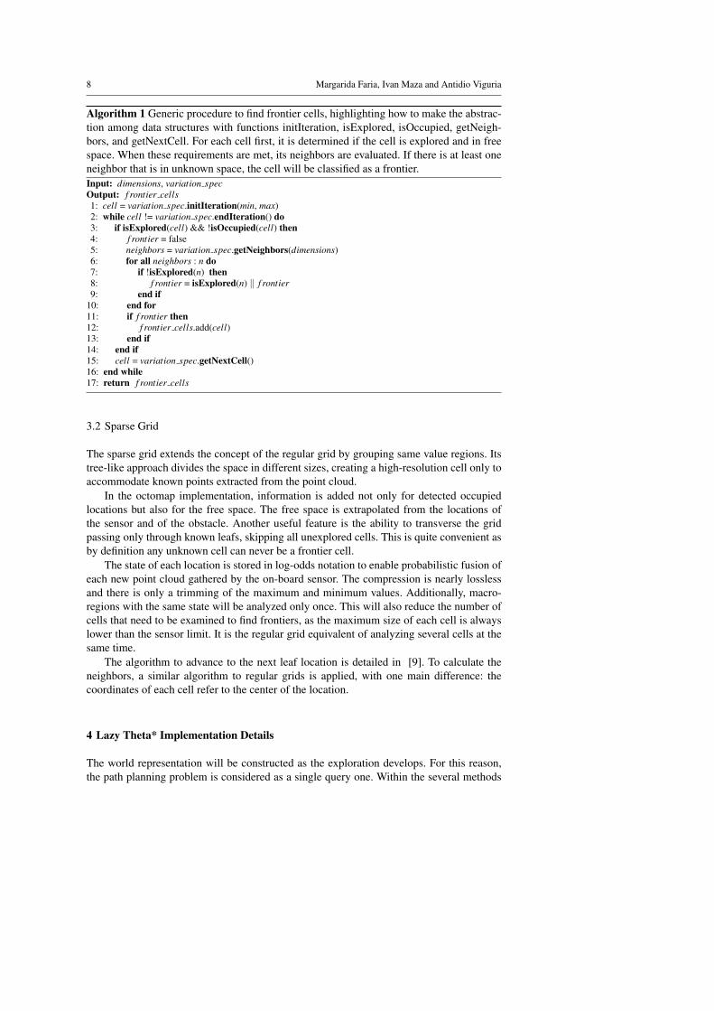
Algorithm 1 Generic procedure to find frontier cells, highlighting how to make the abstrac-tion among data structures with functions initIteration, isExplored, isOccupied, getNeigh-bors, and getNextCell. For each cell first, it is determined if the cell is explored and in freespace. When these requirements are met, its neighbors are evaluated. If there is at least oneneighbor that is in unknown space, the cell will be classified as a frontier.Input: dimensions, variation specOutput: f rontier cells1: cell = variation spec.initIteration(min, max)2: while cell != variation spec.endIteration() do3: if isExplored(cell) && !isOccupied(cell) then4: f rontier = false5: neighbors = variation spec.getNeighbors(dimensions)6: for all neighbors : n do7: if !isExplored(n) then8: f rontier = isExplored(n) ‖ f rontier9: end if

10: end for11: if f rontier then12: f rontier cells.add(cell)13: end if14: end if15: cell = variation spec.getNextCell()16: end while17: return f rontier cells

3.2 Sparse Grid

The sparse grid extends the concept of the regular grid by grouping same value regions. Itstree-like approach divides the space in different sizes, creating a high-resolution cell only toaccommodate known points extracted from the point cloud.

In the octomap implementation, information is added not only for detected occupiedlocations but also for the free space. The free space is extrapolated from the locations ofthe sensor and of the obstacle. Another useful feature is the ability to transverse the gridpassing only through known leafs, skipping all unexplored cells. This is quite convenient asby definition any unknown cell can never be a frontier cell.

The state of each location is stored in log-odds notation to enable probabilistic fusion ofeach new point cloud gathered by the on-board sensor. The compression is nearly losslessand there is only a trimming of the maximum and minimum values. Additionally, macro-regions with the same state will be analyzed only once. This will also reduce the number ofcells that need to be examined to find frontiers, as the maximum size of each cell is alwayslower than the sensor limit. It is the regular grid equivalent of analyzing several cells at thesame time.

The algorithm to advance to the next leaf location is detailed in [9]. To calculate theneighbors, a similar algorithm to regular grids is applied, with one main difference: thecoordinates of each cell refer to the center of the location.

4 Lazy Theta* Implementation Details

The world representation will be constructed as the exploration develops. For this reason,the path planning problem is considered as a single query one. Within the several methods


identified as best performing in single query problems, the Lazy Theta* algorithm was cho-sen both because of the reduced need for post-processing smoothing and the reduced amountof line of sight checks needed. In particular, a variation of the Lazy Theta* algorithm hasbeen implemented and tested with multirotors at the EUROC [45] competition showing itsusability under real-time conditions and realistic constraints. The algorithm is described in[3] as a weighted heuristics to optimize the search space with an asymmetric volume, dueto sensor restrictions. One relevant aspect of the implementation is the different approachesin the global planner and the local planner. The first applies the concept of a regular gridto access neighbors over an octree. The second also employs the idea of a regular grid butover a point cloud. Here the incoming point cloud was refined by removing the outliers andintegrating the sensor error only after multiple confirmations. The local map was further up-dated by eliminating occupied points if no information of them was continuously received.Additionally, replanning is used throughout the mission for optimization purposes. Howeverone of the identified bottlenecks is replanning to overcome large obstacles. This work actsas a follow-up to the promising results presented in [3] for the real-time generation of pathswith obstacle avoidance.

Our implementation of the Lazy Theta* algorithm takes a different approach by directlyimplementing the algorithm over a 3D sparse grid representation of the world. Again, thedata structure used is the octree implementation of the octomap framework. Aiming for animportant reduction of the memory requirements, this will allow sharing the same worldrepresentation for exploration and path planning.

In this work, one of the challenges is to abandon the regular grid mindset entirely totake full advantage of the spacial clustering with sparse grids. The algorithm has been im-plemented in C++ under the Robot Operating System (ROS) [44] as middleware. The opensource implementation is freely available including the unit tests. It is released under theMIT-license and can be obtained from the github project FlyingOctomap3. In the follow-ing the implementation methodology adopted and the adaptation of the algorithm to useOctomap are described.

4.1 Software Implementation Details

One recurring issue in robotics research is the difficulty of gathering the same conditionsover time to reproduce the same experiment. The setup is not straightforward, softwareversions change and the hardware becomes unavailable. Some of these issues have beendealt with in the area of software development and can be mitigated with tools from thatfield. The adoption of software development methodologies, practices and techniques isstarting to spread among the robotics field.

One example is the European project RobMoSys. Some of its key focus is on simpli-fying the setup and configuration software, predictable and traceable properties, certifiablesystems, and better comparability through appropriate metrics (benchmarking) [46]. For theflexible general-purpose modeling of systems, the Unified Modeling Language was taken asreference [47].

Another example is the use of a tool that appeared in the last years as a response tothe continuous integration of software developments, especially in the web developmentarea. This tool is docker. It enables a precise account of all the software packages necessary

3 https://github.com/margaridaCF/FlyingOctomap


to recreate the setup and it is being adopted in robotics: in the ROS build farms, roboticscompanies [48] and even the ROS-Industrial Consortia [49].

An additional example of a technique borrowed from software development is auto-mated testing. To verify that the implementation achieves the intended results under all con-ditions is a non-trivial task. Nowadays frameworks exist to assist in this examination and arecommonly used in software development. It is such a pivotal aspect of development that onemethodology consists of creating tests that show a case where the implementation fails andthen proceeding to improve the implementation until that test no longer fails. This method-ology is called test-driven development. Due to the great number of such tests needed toachieve a complex program they can be automatedly run. Using automated verification, ver-ifying the impact of new development on existing functions becomes trivial. In this context,an edge case is a set of extreme inputs that make a test fail and a scenario is the set of valuesthat compose the pre and post conditions.

The instruments used in our implementation are described in the following.

4.1.1 Variables that compose a scenario

The Lazy Theta* algorithm has as input variables the starting position, the goal position,the world representation, and the number of maximum iterations before declaring a pathunsolvable. The output will be the sequence of waypoints selected to arrive from starting togoal positions.

Some restrictions are enforced over the pre and post conditions. As a precondition toapplying Lazy Theta*, all considered positions must be within the space contemplated inthe world representation. A requirement for the postcondition is that all waypoints must bein free known space.

The starting and goal positions are straightforward to recreate as they are sets of x, yand z coordinates. However, the world representation poses some problems. The variabilityinvolved in generating an octree is tremendous. Each composition of voxel size and quantityhas the potential to be a surprising edge case. Another issue is that it is challenging to setup a well-identified edge case. It would entail manipulating precisely the right sequence ofsensed point clouds to produce the desired octree. Variability was removed by generating theoctree once and then working over a saved, fixed representation. As an additional benefit, italso reduced the time needed to execute a test.

4.1.2 Automate the discovery of edge cases

Another aspect to consider is the verification of edge cases for the different modules of thecode.

To enable the analysis of significant amounts of scenarios, the verification of input andoutput conditions must be automated. Leaping from accessing the specific values for illus-trative scenarios to accessing the whole range of values in a scenario type.

One such type of scenarios is finding a path between two points with a line of sight,which are both in the known space and for which the interval space is also known. The rangeof the input values can be logically asserted as well as the characteristics of the resultingpath, as it can be seen in 4.1.2.

Equipped with these conditions, the whole octree can be searched to find eligible sce-narios. Any case where the preconditions did not generate the expected postconditions isconsidered an error. In the developing phase, this provided the means to search for edge


cases. After their discovery and in accordance with the test-driven development methodol-ogy, they were documented into individual tests. Always in the list of tests used to verifycorrectness. Unfortunately, a similar set of pre and post conditions could not be identified toassess the quality of the generated path while avoiding obstacles.

The ROS integration of Google’s C++ unit testing framework gtest [50] is the tool usedfor automated unit testing.

Algorithm 2 Pre and post conditions for a solution to be considered correct for the simpleuse case.

Start is the starting position.Goal is the final position.World is set of all voxels contained in the octree.v represents an analyzed voxel.‖ StartGoal ‖ is fixed for each test set.resultingPath set of all waypoints that compose the solution

Require:Start ∈WorldFreeGoal ∈WorldFreeStartGoal ∈WorldFreeAndKnown∀v,vneighbors ∈WorldKnown

Ensure:resultingPath.size == 2‖ resultingPath[2]toVoxelCenter(goal) ‖< resultingPath[2].size‖ resultingPath[1]toVoxelCenter(start) ‖< resultingPath[1].size

4.1.3 Automated assertion of correctness

The amount of test cases and operations involved in the algorithm rapidly generated a hugeamount of tests. This is the main reason that motivated the adoption of test-driven program-ming as the development process of the implementation, hence automating the tests.

For each foreseeable use case, there is a suite of unit tests. Each test considers startconditions in a homogenous way supported by the well-defined input elements that define ascenario.

While testing the code in simulation, inputting commands to the UAS quickly provedinefficient. With scripted starting conditions and a manual input of the commands, there wastoo much variability. An option was to use scripted commands however it still required toomuch time to complete the tests. Instead, all the components of the scenario are numericallydefined for each test case.

4.1.4 Direct pseudo-code to code translation

Frugality is a recognized challenge as it can be seen in the implementation related in [3]where both locally implemented regular grids and the raw point cloud as supplied in thePCL library were needed.

The code was developed as a direct, unmodified (except in heuristics as seen in thesection 4.2.4) implementation of Lazy Theta* as found on [35]. To efficiently verify thisclaim, each line of the pseudocode is included as a comment above its implementation. Theimplementation is done to encapsulate technical details and highlight the logic. The precise


correlation between code and pseudo code proved crucial in the later stages of implementa-tion to verify its correctness.

4.1.5 Statistical analysis of results

The same automation used to look for edge cases can be used later to analyze the perfor-mance of the implementation statistically. This feature was identified in [3] as bringingsubstantial insight.

As a follow-up of an implementation that relies on regular grids, it is interesting tounderstand how the sparse grid correlates to a regular grid regarding number of iterations.The results are detailed in section 5.2.3.

4.2 Adapting Lazy Theta* to Octomap

As it was identified in [7], the primitives on which the algorithms are based have a deter-minant role in the performance of the final solution. This primitives are the direct connec-tion between the algorithm and the environment representation. Critical primitives in LazyTheta* related in [35] are: uniquely identifying a voxel, finding a voxel’s size and finding avoxel’s neighbors.

Even though one of the goals pursued in this research is to lighten the memory footprint,one challenge to apply this algorithm to the octree was precisely its lightness. Each node hasvery little information: only a pointer to an array of higher resolution voxels that form thesame volume and an identifier for within a tree level. In the octomap implementation, a nodehas the highest resolution for its location when its pointer to children is NULL.

The tree depth of an octree is fixed from its creation. As the authors of the octomap noteat [9], a maximum depth of 16 is sufficient to cover a cube with a volume of 655.36 m3 atone centimeter resolution. For this implementation, a resolution of 20 cm was considered,making a maximum depth of 16 sufficient for a volume of 1310720 m3.

4.2.1 Voxel Identification

Coordinates keys cannot uniquely identify each voxel of the octree since coordinates over-lap. Each voxel is contained by a bigger one, except for the root node. The identifier with alevel is not globally unique either. Apart from the node state, there is no other informationassociated with each node.

The solution was to use the coordinates of the center of the voxel associated with thevoxel size. This creates a composite key4 that is unique accross the tree.

4.2.2 Voxel Size

Both associated to the voxel identification and finding neighbors, voxel size is crucial todeduct the size of the highest resolution voxel containing a given random point.

Given a coordinate point, finding the size of the associated leaf node has a complexity ofO(tree depth). Starting from the root of the tree (which is the node of minimum resolution

4 A concept borrowed from relational databases. A composite key is a combination of two or more char-acteristics of an instance that can be used to uniquely identify it. However, when they are taken individuallydo not guarantee uniqueness.


/ maximum volume), each tree level must be transversed analyzing the subsequently smallersize voxels that contain the target point until a leaf node is found.

4.2.3 Voxel Neighbours

The sparseness of the tree makes finding a voxel’s neighbors nontrivial. In [3] the approachwas to create a local regular grid and discard the size of the analyzed voxel. In practice, it asif a local potential field was created with the goal as an attractor and the voxel dimensions asboundaries. Only while analyzing positions within the same voxel, the result obtained wasthe same as by finding the neighboring voxel of the octomap through steepest descent (ofthe distance to the goal).

To take advantage of the organization in the octree and jump directly to the next neigh-bors, all possible combinations between the voxels’ size and its neighbor’s size must becontemplated. Voxels with large neighbors will have a smaller set of neighbors. Voxels sur-rounded by voxels of maximum resolution will have more neighbors.

As in frontier cells exploration, diagonal neighbors are not contemplated. A voxel ofmaximum resolution has six neighbors. While a voxel twice the maximum resolution has amaximum of twenty-four neighbors.

To compile the list of neighbors of a random point the following steps are followed:

1. Find unique identifier within tree level2. Find node level in octree3. Find voxel size4. Calculate the coordinates of the center of each neighbor assuming all neighbors have

the maximum resolution. The center coordinates of a neighbor will only be added once.This verification has complexity of O((node size/resolution)2).

4.2.4 Heuristic adaptation to the sparse grid

In [35], the voxel’s vertices are the intended candidates for waypoints. However, for thereasons mentioned before, the voxel center’s are the coordinates being used as waypointcandidates in this implementation.

The heuristics to manage the list of candidate waypoints (or the open list) is ordered byg(s)+h(s) with the following definitions:

For every vertex s the g-value g(s) is the length of the shortest path from sstart to sfound so far. [35, p. 3]

We use the straight line distances c(s,sgoal) as h-values in our experiments. [35, p. 5]

On one hand, the original assumption of a regular grid in [35] no longer holds. Onthe other hand, instead of having many points as waypoint candidates for each voxel (eachvertex), now there is only one (the center). From here follows that the distance between thegoal point and its voxel center can be significant. This offset will impact the efficiency ofthe heuristics if left unmodified.

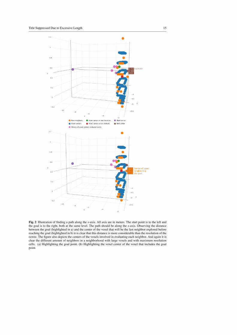
In order to illustrate this case the scenario depicted in Fig. 2 will be considered 5. Thestart point is to the left and the goal is to the right, both at the same level. The path should be

5 octree offShoreOil 1m.bt (available at https://github.com/margaridaCF/dataStructureAnalysis), withstart point (-11.3m, -4.9m, 0.5m) and goal point (-1.3m, -4.9m, 0.5m)


Room Corridor Z shape 2 pillars 4 pillars PillarsWidth (m) 24 24 22 77.8 180.4 13

Length (m) 8 14 13.8 77.2 90 10

Table 1 Size of the scenarios in Fig. 4 used in the simulations.

along the x-axis. This edge case can arise in situations where the goal position is containedby a voxel that has large voxels in its neighborhood. Observing the distance between thegoal (highlighted in a) and the center of the voxel that will be the last neighbor exploredbefore reaching the goal (highlighted in b), it is clear that distance between these two pointsis larger than the resolution of the octree. This throws off the heuristic because many smallerneighbors will be found that have a smaller distance to the goal but are not in the directionof the goal. What happens in this run is the following. At iteration 220, the final voxel isfound. However, as it is a large voxel, it will be left near the bottom of the priority queueof nodes to evaluate (at position 173) and it will take many iterations before the algorithmstudies this particular option. This is as noticeable as the offset between the goal point andits voxel center.

In order to address this issue, the heuristic function was changed from the continuousfunction exposed before to a piecewise function with 0 as the result for the voxel that con-tains the goal point. While this might lead to slightly suboptimal paths, it was considered afair trade-off.

5 Results and analysis

The results and their analysis for frontier cells exploration and path planning with LazyTheta* are described in the following.

5.1 Frontier Cells Exploration

The exploration algorithm of frontier cells was first tested in a simulated environment andlater with octrees constructed by an UAS in an experimental setting.

5.1.1 Simulation Environment

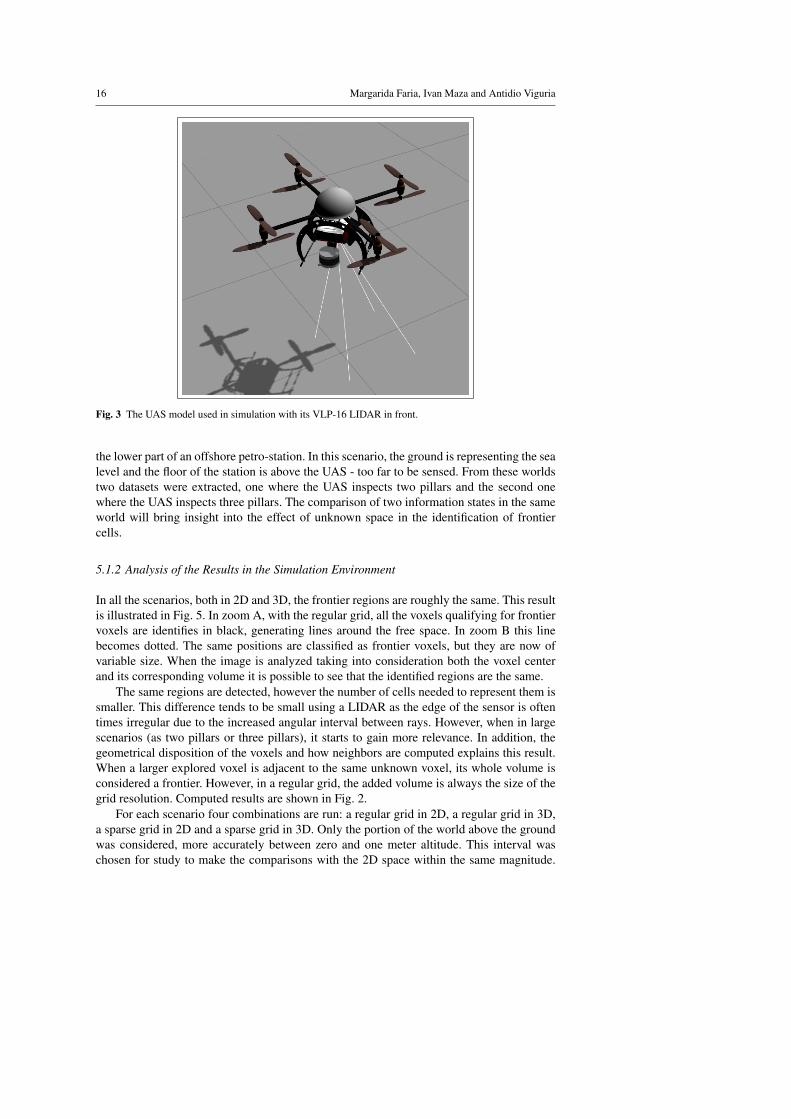
Five datasets were used to run the tests in simulation. They were all generated using ROSnodes on a Gazebo simulator. The sensor used emulates a VLP-16 LIDAR: it is omnidirec-tional, dividing the 360 degrees into 1500 samples and stacking it 16 times. The sensor wasmounted on the front of the 3D model of a quadrotor (see Fig. 3).

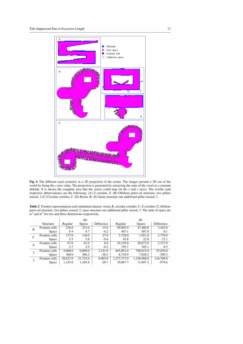
Five simulated worlds have been considered. They are shown in Fig. 4, where the imagesrepresent a 2D cut of the world by fixing the z-axis value. Three of them are the same asthe ones used in [51]: an enclosed space with only one opening6 (room), a circular corridorwith one opening to the inner area and a Z shaped corridor with openings at both ends. Inthese scenarios the UAS fully explores the enclosed area, never crossing an opening. Eachof the openings is 0.8 meters long. The dimensions of the simulated worlds are detailed inTable 5.1.1. For a scale closer to the targeted application, there is a scenario that emulates

6 Opening is used in the sense of a break in a continuous wall.


Fig. 2 Illustration of finding a path along the x-axis. All axis are in meters. The start point is to the left andthe goal is to the right, both at the same level. The path should be along the x-axis. Observing the distancebetween the goal (highlighted in a) and the center of the voxel that will be the last neighbor explored beforereaching the goal (highlighted in b) it is clear that this distance is more considerable than the resolution of theoctree. The figure also depicts the centers of the voxels involved in evaluating each neighbor. And again it isclear the different amount of neighbors in a neighborhood with large voxels and with maximum resolutioncells. (a) Highlighting the goal point. (b) Highlighting the voxel center of the voxel that includes the goalpoint.


Fig. 3 The UAS model used in simulation with its VLP-16 LIDAR in front.

the lower part of an offshore petro-station. In this scenario, the ground is representing the sealevel and the floor of the station is above the UAS - too far to be sensed. From these worldstwo datasets were extracted, one where the UAS inspects two pillars and the second onewhere the UAS inspects three pillars. The comparison of two information states in the sameworld will bring insight into the effect of unknown space in the identification of frontiercells.

5.1.2 Analysis of the Results in the Simulation Environment

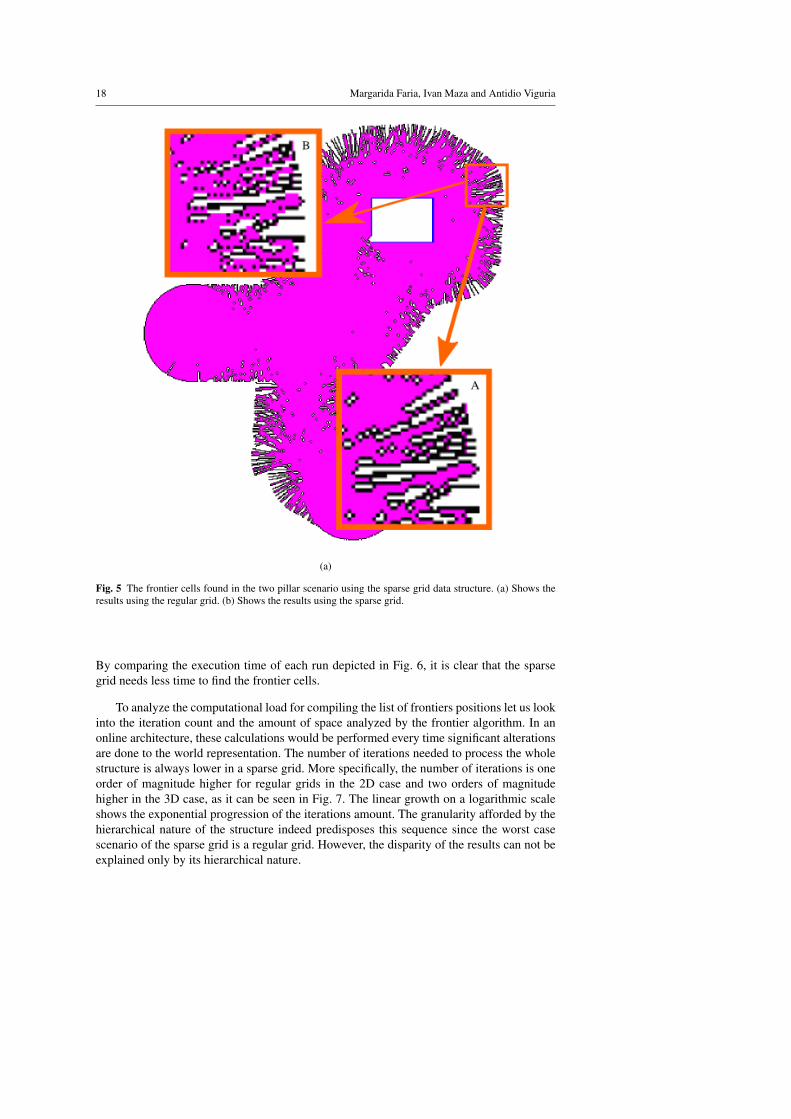
In all the scenarios, both in 2D and 3D, the frontier regions are roughly the same. This resultis illustrated in Fig. 5. In zoom A, with the regular grid, all the voxels qualifying for frontiervoxels are identifies in black, generating lines around the free space. In zoom B this linebecomes dotted. The same positions are classified as frontier voxels, but they are now ofvariable size. When the image is analyzed taking into consideration both the voxel centerand its corresponding volume it is possible to see that the identified regions are the same.

The same regions are detected, however the number of cells needed to represent them issmaller. This difference tends to be small using a LIDAR as the edge of the sensor is oftentimes irregular due to the increased angular interval between rays. However, when in largescenarios (as two pillars or three pillars), it starts to gain more relevance. In addition, thegeometrical disposition of the voxels and how neighbors are computed explains this result.When a larger explored voxel is adjacent to the same unknown voxel, its whole volume isconsidered a frontier. However, in a regular grid, the added volume is always the size of thegrid resolution. Computed results are shown in Fig. 2.

For each scenario four combinations are run: a regular grid in 2D, a regular grid in 3D,a sparse grid in 2D and a sparse grid in 3D. Only the portion of the world above the groundwas considered, more accurately between zero and one meter altitude. This interval waschosen for study to make the comparisons with the 2D space within the same magnitude.


Fig. 4 The different used scenarios in a 2D projection of the octree. The images present a 2D cut of theworld by fixing the z-axis value. The projection is generated by extracting the state of the voxel at a constantaltitude. It is shown the complete area that the octree could map (in the x and y axes). The worlds (andrespective abbreviations) are the following: (A) Z corridor, Z. (B) Offshore petro-oil structure, two pillarssensed. 2 (C) Circular corridor, C. (D) Room, R. (E) Same structure one additional pillar sensed, 3.

Table 2 Frontier representation each simulation dataset: room, R; circular corridor, C; Z corridor, Z; offshorepetro-oil structure, two pillars sensed, 2; same structure one additional pillar sensed, 3. The units of space arem2 and m3 for two and three dimensions respectively.

2D 3DStructure Regular Sparse Difference Regular Sparse Difference

R Frontier cells 236.0 221.0 15.0 50,903.0 47,460.0 3,443.0Space 9.4 9.7 -0.2 407.1 407.0 0.1

C Frontier cells 137.0 110.0 27.0 5,729.0 1,951.0 3,778.0Space 5.5 5.8 -0.4 45.8 22.8 23.1

Z Frontier cells 67.0 61.0 6.0 24,210.0 20,873.0 3,337.0Space 2.7 2.9 -0.2 193.7 185.1 8.5

2 Frontier cells 9,000.0 6,809.0 2,191.0 845,091.0 790,015.0 55,076.0Space 360.0 386.2 -26.2 6,718.9 7,028.2 -309.3

3 Frontier cells 28,627.0 21,724.0 6,903.0 1,273,737.0 1,156,968.0 116,769.0Space 1,145.0 1,165.6 -20.7 10,067.7 11,047.3 -979.6


(a)

Fig. 5 The frontier cells found in the two pillar scenario using the sparse grid data structure. (a) Shows theresults using the regular grid. (b) Shows the results using the sparse grid.

By comparing the execution time of each run depicted in Fig. 6, it is clear that the sparsegrid needs less time to find the frontier cells.

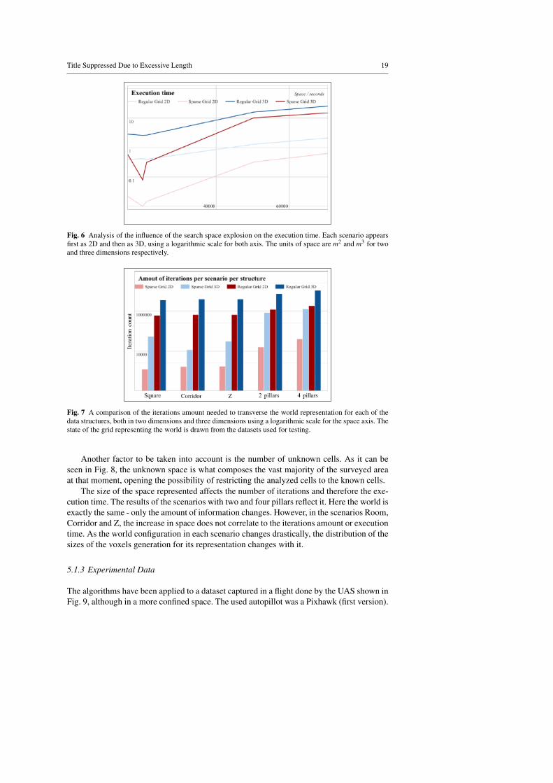
To analyze the computational load for compiling the list of frontiers positions let us lookinto the iteration count and the amount of space analyzed by the frontier algorithm. In anonline architecture, these calculations would be performed every time significant alterationsare done to the world representation. The number of iterations needed to process the wholestructure is always lower in a sparse grid. More specifically, the number of iterations is oneorder of magnitude higher for regular grids in the 2D case and two orders of magnitudehigher in the 3D case, as it can be seen in Fig. 7. The linear growth on a logarithmic scaleshows the exponential progression of the iterations amount. The granularity afforded by thehierarchical nature of the structure indeed predisposes this sequence since the worst casescenario of the sparse grid is a regular grid. However, the disparity of the results can not beexplained only by its hierarchical nature.


Fig. 6 Analysis of the influence of the search space explosion on the execution time. Each scenario appearsfirst as 2D and then as 3D, using a logarithmic scale for both axis. The units of space are m2 and m3 for twoand three dimensions respectively.

Fig. 7 A comparison of the iterations amount needed to transverse the world representation for each of thedata structures, both in two dimensions and three dimensions using a logarithmic scale for the space axis. Thestate of the grid representing the world is drawn from the datasets used for testing.

Another factor to be taken into account is the number of unknown cells. As it can beseen in Fig. 8, the unknown space is what composes the vast majority of the surveyed areaat that moment, opening the possibility of restricting the analyzed cells to the known cells.

The size of the space represented affects the number of iterations and therefore the exe-cution time. The results of the scenarios with two and four pillars reflect it. Here the world isexactly the same - only the amount of information changes. However, in the scenarios Room,Corridor and Z, the increase in space does not correlate to the iterations amount or executiontime. As the world configuration in each scenario changes drastically, the distribution of thesizes of the voxels generation for its representation changes with it.

5.1.3 Experimental Data

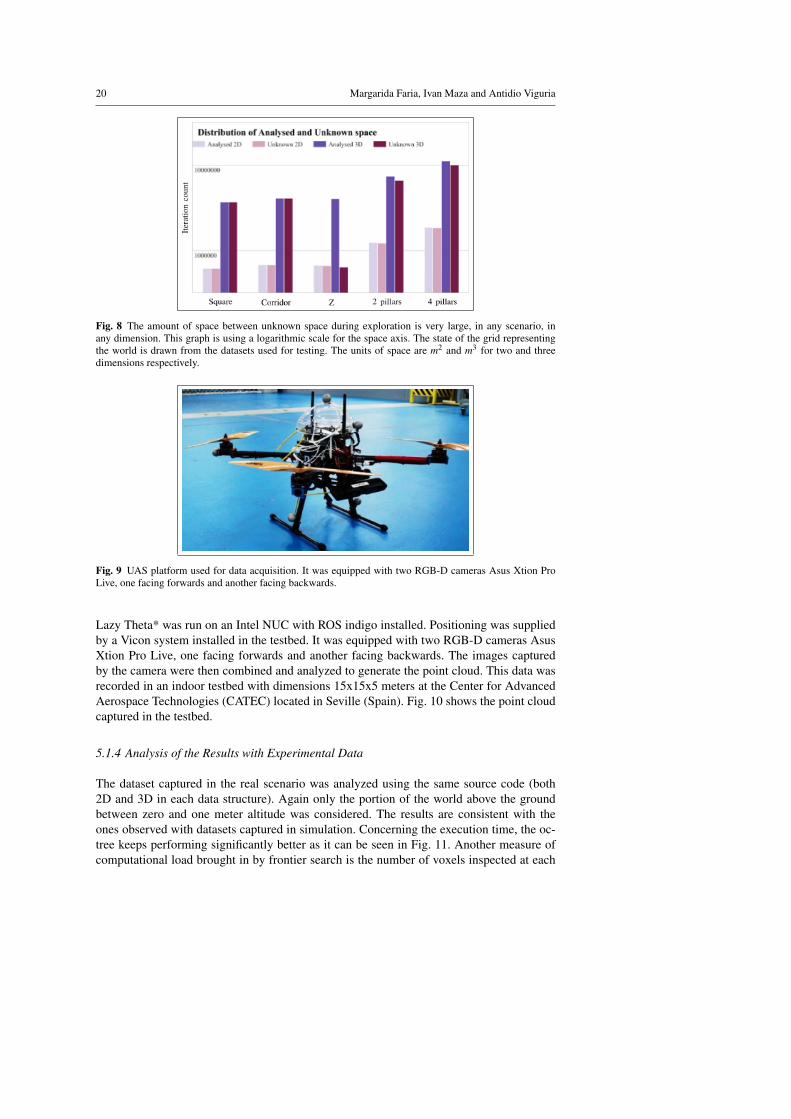
The algorithms have been applied to a dataset captured in a flight done by the UAS shown inFig. 9, although in a more confined space. The used autopillot was a Pixhawk (first version).


Fig. 8 The amount of space between unknown space during exploration is very large, in any scenario, inany dimension. This graph is using a logarithmic scale for the space axis. The state of the grid representingthe world is drawn from the datasets used for testing. The units of space are m2 and m3 for two and threedimensions respectively.

Fig. 9 UAS platform used for data acquisition. It was equipped with two RGB-D cameras Asus Xtion ProLive, one facing forwards and another facing backwards.

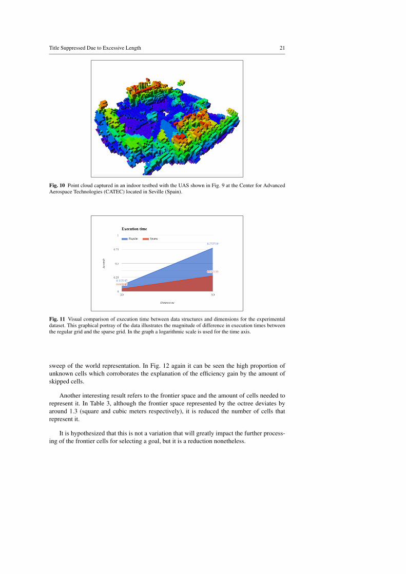
Lazy Theta* was run on an Intel NUC with ROS indigo installed. Positioning was suppliedby a Vicon system installed in the testbed. It was equipped with two RGB-D cameras AsusXtion Pro Live, one facing forwards and another facing backwards. The images capturedby the camera were then combined and analyzed to generate the point cloud. This data wasrecorded in an indoor testbed with dimensions 15x15x5 meters at the Center for AdvancedAerospace Technologies (CATEC) located in Seville (Spain). Fig. 10 shows the point cloudcaptured in the testbed.

5.1.4 Analysis of the Results with Experimental Data

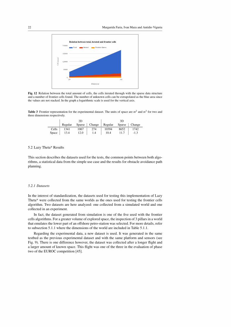
The dataset captured in the real scenario was analyzed using the same source code (both2D and 3D in each data structure). Again only the portion of the world above the groundbetween zero and one meter altitude was considered. The results are consistent with theones observed with datasets captured in simulation. Concerning the execution time, the oc-tree keeps performing significantly better as it can be seen in Fig. 11. Another measure ofcomputational load brought in by frontier search is the number of voxels inspected at each


Fig. 10 Point cloud captured in an indoor testbed with the UAS shown in Fig. 9 at the Center for AdvancedAerospace Technologies (CATEC) located in Seville (Spain).

Fig. 11 Visual comparison of execution time between data structures and dimensions for the experimentaldataset. This graphical portray of the data illustrates the magnitude of difference in execution times betweenthe regular grid and the sparse grid. In the graph a logarithmic scale is used for the time axis.

sweep of the world representation. In Fig. 12 again it can be seen the high proportion ofunknown cells which corroborates the explanation of the efficiency gain by the amount ofskipped cells.

Another interesting result refers to the frontier space and the amount of cells needed torepresent it. In Table 3, although the frontier space represented by the octree deviates byaround 1.3 (square and cubic meters respectively), it is reduced the number of cells thatrepresent it.

It is hypothesized that this is not a variation that will greatly impact the further process-ing of the frontier cells for selecting a goal, but it is a reduction nonetheless.


Fig. 12 Relation between the total amount of cells, the cells iterated through with the sparse data structureand a number of frontier cells found. The number of unknown cells can be extrapolated as the blue area sincethe values are not stacked. In the graph a logarithmic scale is used for the vertical axis.

Table 3 Frontier representation for the experimental dataset. The units of space are m2 and m3 for two andthree dimensions respectively.

2D 3DRegular Sparse Change Regular Sparse Change

Cells 1341 1067 274 10394 8652 1742Space 13.4 12.0 1.4 10.4 11.7 -1.3

5.2 Lazy Theta* Results

This section describes the datasets used for the tests, the common points between both algo-rithms, a statistical data from the simple use case and the results for obstacle avoidance pathplanning.

5.2.1 Datasets

In the interest of standardization, the datasets used for testing this implementation of LazyTheta* were collected from the same worlds as the ones used for testing the frontier cellsalgorithm. Two datasets are here analyzed: one collected from a simulated world and onecollected in an experiment.

In fact, the dataset generated from simulation is one of the five used with the frontiercells algorithms. For a greater volume of explored space, the inspection of 3 pillars in a worldthat emulates the lower part of an offshore petro-station was selected. For more details, referto subsection 5.1.1 where the dimensions of the world are included in Table 5.1.1.

Regarding the experimental data, a new dataset is used. It was generated in the sametestbed as the previous experimental dataset and with the same platform and sensors (seeFig. 9). There is one difference however, the dataset was collected after a longer flight anda larger amount of known space. This flight was one of the three in the evaluation of phasetwo of the EUROC competition [45].


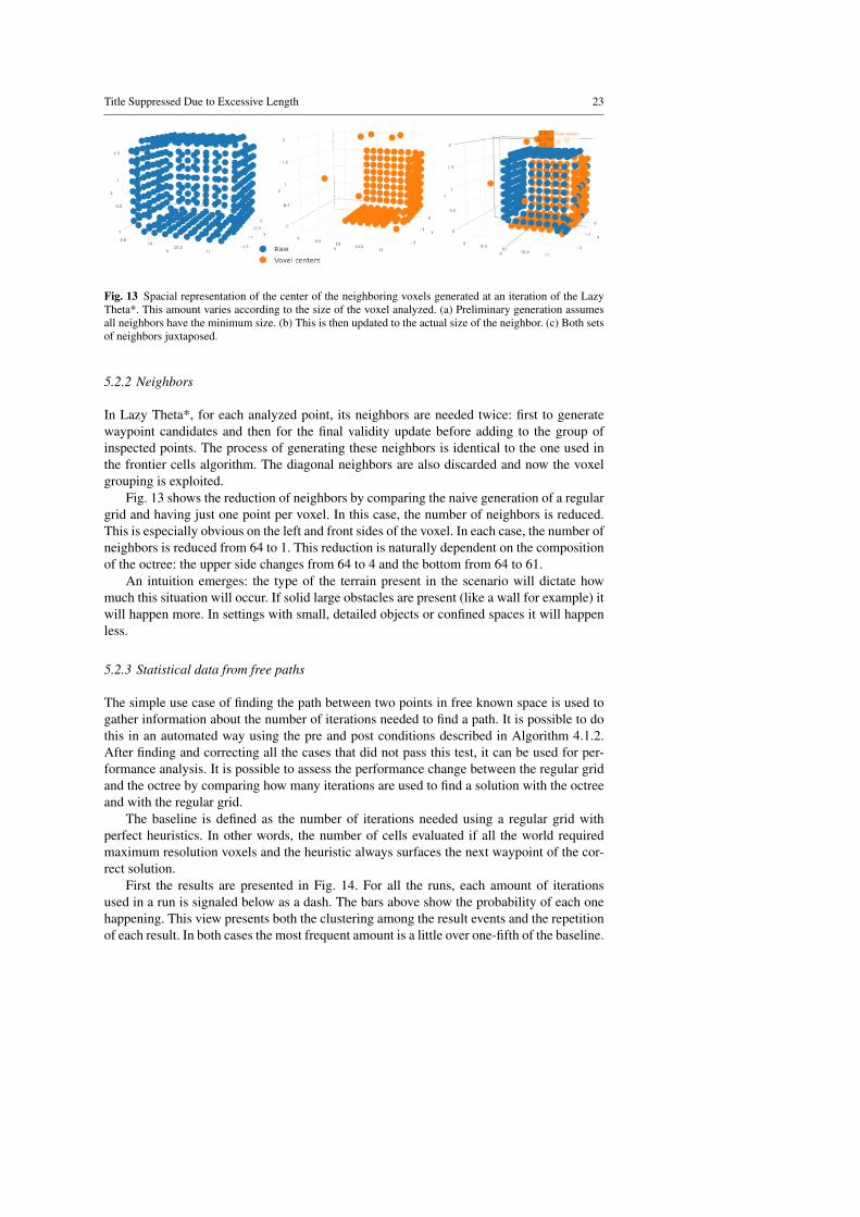
Fig. 13 Spacial representation of the center of the neighboring voxels generated at an iteration of the LazyTheta*. This amount varies according to the size of the voxel analyzed. (a) Preliminary generation assumesall neighbors have the minimum size. (b) This is then updated to the actual size of the neighbor. (c) Both setsof neighbors juxtaposed.

5.2.2 Neighbors

In Lazy Theta*, for each analyzed point, its neighbors are needed twice: first to generatewaypoint candidates and then for the final validity update before adding to the group ofinspected points. The process of generating these neighbors is identical to the one used inthe frontier cells algorithm. The diagonal neighbors are also discarded and now the voxelgrouping is exploited.

Fig. 13 shows the reduction of neighbors by comparing the naive generation of a regulargrid and having just one point per voxel. In this case, the number of neighbors is reduced.This is especially obvious on the left and front sides of the voxel. In each case, the number ofneighbors is reduced from 64 to 1. This reduction is naturally dependent on the compositionof the octree: the upper side changes from 64 to 4 and the bottom from 64 to 61.

An intuition emerges: the type of the terrain present in the scenario will dictate howmuch this situation will occur. If solid large obstacles are present (like a wall for example) itwill happen more. In settings with small, detailed objects or confined spaces it will happenless.

5.2.3 Statistical data from free paths

The simple use case of finding the path between two points in free known space is used togather information about the number of iterations needed to find a path. It is possible to dothis in an automated way using the pre and post conditions described in Algorithm 4.1.2.After finding and correcting all the cases that did not pass this test, it can be used for per-formance analysis. It is possible to assess the performance change between the regular gridand the octree by comparing how many iterations are used to find a solution with the octreeand with the regular grid.

The baseline is defined as the number of iterations needed using a regular grid withperfect heuristics. In other words, the number of cells evaluated if all the world requiredmaximum resolution voxels and the heuristic always surfaces the next waypoint of the cor-rect solution.

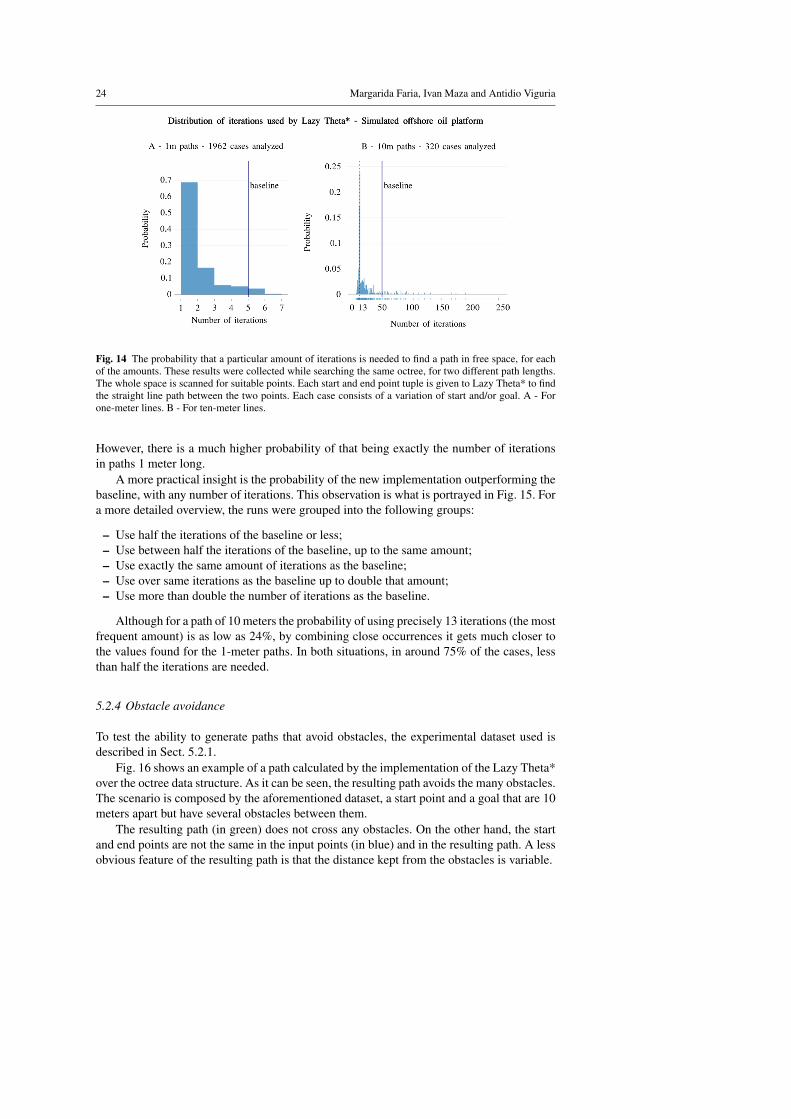
First the results are presented in Fig. 14. For all the runs, each amount of iterationsused in a run is signaled below as a dash. The bars above show the probability of each onehappening. This view presents both the clustering among the result events and the repetitionof each result. In both cases the most frequent amount is a little over one-fifth of the baseline.


Fig. 14 The probability that a particular amount of iterations is needed to find a path in free space, for eachof the amounts. These results were collected while searching the same octree, for two different path lengths.The whole space is scanned for suitable points. Each start and end point tuple is given to Lazy Theta* to findthe straight line path between the two points. Each case consists of a variation of start and/or goal. A - Forone-meter lines. B - For ten-meter lines.

However, there is a much higher probability of that being exactly the number of iterationsin paths 1 meter long.

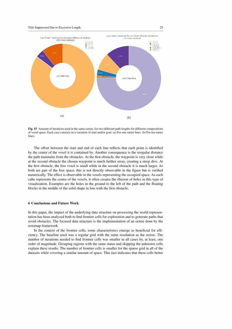
A more practical insight is the probability of the new implementation outperforming thebaseline, with any number of iterations. This observation is what is portrayed in Fig. 15. Fora more detailed overview, the runs were grouped into the following groups:

– Use half the iterations of the baseline or less;– Use between half the iterations of the baseline, up to the same amount;– Use exactly the same amount of iterations as the baseline;– Use over same iterations as the baseline up to double that amount;– Use more than double the number of iterations as the baseline.

Although for a path of 10 meters the probability of using precisely 13 iterations (the mostfrequent amount) is as low as 24%, by combining close occurrences it gets much closer tothe values found for the 1-meter paths. In both situations, in around 75% of the cases, lessthan half the iterations are needed.

5.2.4 Obstacle avoidance

To test the ability to generate paths that avoid obstacles, the experimental dataset used isdescribed in Sect. 5.2.1.

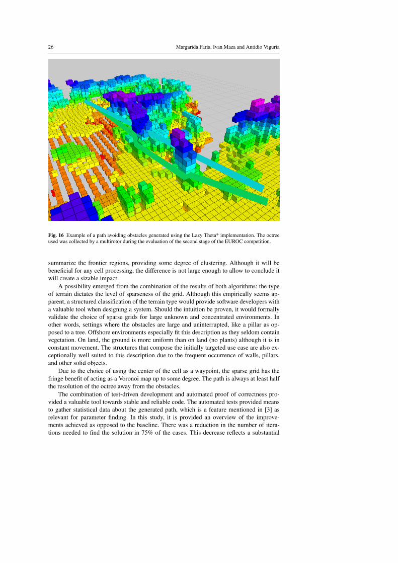
Fig. 16 shows an example of a path calculated by the implementation of the Lazy Theta*over the octree data structure. As it can be seen, the resulting path avoids the many obstacles.The scenario is composed by the aforementioned dataset, a start point and a goal that are 10meters apart but have several obstacles between them.

The resulting path (in green) does not cross any obstacles. On the other hand, the startand end points are not the same in the input points (in blue) and in the resulting path. A lessobvious feature of the resulting path is that the distance kept from the obstacles is variable.


(a) (b)

Fig. 15 Amount of iterations used in the same octree, for two different path lengths for different compositionsof voxel space. Each case consists on a variation of start and/or goal. (a) For one meter lines. (b) For ten meterlines.

The offset between the start and end of each line reflects that each point is identifiedby the center of the voxel it is contained by. Another consequence is the irregular distancethe path maintains from the obstacles. At the first obstacle, the waypoint is very close whileat the second obstacle the chosen waypoint is much further away, creating a steep dive. Atthe first obstacle, the free voxel is small while in the second obstacle it is much larger. Asboth are part of the free space, this is not directly observable in the figure but is verifiednumerically. The effect is observable in the voxels representing the occupied space. As eachcube represents the center of the voxels, it often creates the illusion of holes in this type ofvisualization. Examples are the holes in the ground to the left of the path and the floatingblocks in the middle of the solid shape in line with the first obstacle.

6 Conclusions and Future Work

In this paper, the impact of the underlying data structure on processing the world represen-tation has been analyzed both to find frontier cells for exploration and to generate paths thatavoid obstacles. The focused data structure is the implementation of an octree done by theoctomap framework.

In the context of the frontier cells, some characteristics emerge as beneficial for effi-ciency. The baseline used was a regular grid with the same resolution as the octree. Thenumber of iterations needed to find frontier cells was smaller in all cases by, at least, oneorder of magnitude. Grouping regions with the same status and skipping the unknown cellsexplain these results. The number of frontier cells is smaller for the sparse grid in all of thedatasets while covering a similar amount of space. This fact indicates that these cells better


Fig. 16 Example of a path avoiding obstacles generated using the Lazy Theta* implementation. The octreeused was collected by a multirotor during the evaluation of the second stage of the EUROC competition.

summarize the frontier regions, providing some degree of clustering. Although it will bebeneficial for any cell processing, the difference is not large enough to allow to conclude itwill create a sizable impact.

A possibility emerged from the combination of the results of both algorithms: the typeof terrain dictates the level of sparseness of the grid. Although this empirically seems ap-parent, a structured classification of the terrain type would provide software developers witha valuable tool when designing a system. Should the intuition be proven, it would formallyvalidate the choice of sparse grids for large unknown and concentrated environments. Inother words, settings where the obstacles are large and uninterrupted, like a pillar as op-posed to a tree. Offshore environments especially fit this description as they seldom containvegetation. On land, the ground is more uniform than on land (no plants) although it is inconstant movement. The structures that compose the initially targeted use case are also ex-ceptionally well suited to this description due to the frequent occurrence of walls, pillars,and other solid objects.

Due to the choice of using the center of the cell as a waypoint, the sparse grid has thefringe benefit of acting as a Voronoi map up to some degree. The path is always at least halfthe resolution of the octree away from the obstacles.

The combination of test-driven development and automated proof of correctness pro-vided a valuable tool towards stable and reliable code. The automated tests provided meansto gather statistical data about the generated path, which is a feature mentioned in [3] asrelevant for parameter finding. In this study, it is provided an overview of the improve-ments achieved as opposed to the baseline. There was a reduction in the number of itera-tions needed to find the solution in 75% of the cases. This decrease reflects a substantial


amount of different configurations of the underlying octree that leads to a reduction of thenecessary computational power. Here the baseline is equivalent to how many voxels wouldbe evaluated if all the space required maximum resolution voxels and the heuristic alwayssurfaced the next waypoint of the correct solution. These results are explained by the abilityto evaluate several (maximum resolution and same state) voxels at a time. This capabilityavoids the evaluation of each one individually.

The effort to encapsulate technical details in higher level structures made possible asemantic level of inspection of the code. This insight allowed to identify some initial mis-interpretations and enabled the certification that the algorithm was indeed implemented asintended.

Several different future directions of research are of interest. On one hand, it would beof great benefit to integrate more data structures and to add more implementations of theoctree such as the PCL cloud. On the other hand, it would be valuable to compare entirelydifferent data structures. One type of data structure of particular interest is a triangle meshextracted with Delaunay triangulation. Again several implementations exist (CGAL, PCL),and comparing them would bring greater insight into their application. Another researchdirection is to evaluate the performance of the search algorithm throughout a mission. Suchsurvey would permit a thorough comparison between increasing amounts of information inthe same scenario while using each different data structure. Finally, our mid-term objectiveis to apply these results to UAS exploring extensive areas in real-time. With the combinationof exploration and path planning, the UAS would be able to detect when all reachable pointcloud information had been sampled and autonomously deliberate to stop.

References

1. Armin Hornung et al. Octomap. [Online; accessed 28 sep 2017].2. M. Faria, I. Maza, and A. Viguria. Analysis of data structures and exploration techniques applied to

large 3D marine structures using UAS. In 2017 International Conference on Unmanned Aircraft Systems(ICUAS), pages 1277–1284, June 2017.

3. Francisco J Perez-grau, Fernando Caballero, Ricardo Ragel, Antidio Viguria, and Anibal Ollero. AnArchitecture for Robust UAV Navigation in GPS-denied Areas. Journal of Field Robotics (JFR), SpecialIssue on High Speed Vision-Based Autonomous UAVs, 2017.

4. Samuel Hornus, Olivier Devillers, and Clement Jamin. dD triangulations. In CGAL User and ReferenceManual. CGAL Editorial Board, 4.9 edition, 2016.

5. Flemming Schøler, Morten Bisgaard, and Anders Cour-harbo. Generating Configuration Spaces andVisibility Graphs from a Geometric Workspace for UAV Path Planning. Autonomous Robots, pages1–14, 2013.

6. Rosli Omar and Rosli Omar. PATH PLANNING FOR UNMANNED AERIAL VEHICLES USINGVISIBILITY LINE-BASED METHODS Thesis submitted for the degree of Doctor of Philosophy at theUniversity of Leicester by Department of Engineering VISIBILITY LINE-BASED METHOD. (March),2011.

7. Steven M. LaValle. Planning algorithms. Planning Algorithms, 9780521862059:1–826, 2006.8. Alexander Greß and Reinhard Klein. Efficient representation and extraction of 2-manifold isosurfaces

using kd-trees. Graphical Models, 66(6):370–397, 2004.9. Armin Hornung, Kai M. Wurm, Maren Bennewitz, Cyrill Stachniss, and Wolfram Burgard. OctoMap:

An efficient probabilistic 3D mapping framework based on octrees. Autonomous Robots, 34(3):189–206,2013.

10. Radu Bogdan Rusu and Steve Cousins. 3D is here: Point Cloud Library (PCL). In IEEE InternationalConference on Robotics and Automation (ICRA), Shanghai, China, May 9-13 2011.

11. Sebastian Thrun, Wolfram Burgard, and Dieter Fox. Probabilistic robotics. Intelligent robotics andautonomous agents. The MIT Press, Cambridge (Mass.) (London), 2005.

12. Brian Yamauchi. A frontier-based approach for autonomous exploration. In Proceedings 1997 IEEEInternational Symposium on Computational Intelligence in Robotics and Automation CIRA’97. ’TowardsNew Computational Principles for Robotics and Automation’, pages 146–151. IEEE Comput. Soc. Press,1997.


13. Friedrich Fraundorfer, Lionel Heng, Dominik Honegger, Gim Hee Lee, Lorenz Meier, Petri Tanskanen,and Marc Pollefeys. Vision-based autonomous mapping and exploration using a quadrotor MAV. IEEEInternational Conference on Intelligent Robots and Systems, pages 4557–4564, 2012.

14. Leonardo Romero, Eduardo Morales, and Enrique Sucar. A Robust Exploration and Navigation Ap-proach for Indoor Mobile Robots Merging Local and Global Strategies. Advances in Artificial Intelli-gence: International Joint Conference 7th Ibero-American Conference on AI 15th Brazilian Symposiumon AI IBERAMIA-SBIA 2000 Atibaia, SP, Brazil, November 19–22, 2000 Proceedings, pages 389–398,2000.

15. Christian Dornhege and Alexander Kleiner. A frontier-void-based approach for autonomous explorationin 3d. In 2011 IEEE International Symposium on Safety, Security, and Rescue Robotics, pages 351–356.IEEE, nov 2011.

16. Gavin Paul, Stephen Webb, Dikai Liu, and Gamini Dissanayake. Autonomous robot manipulator-basedexploration and mapping system for bridge maintenance. Robotics and Autonomous Systems, 59(7-8):543–554, 2011.

17. Christian Potthast and Gaurav S. Sukhatme. A probabilistic framework for next best view estimation ina cluttered environment. Journal of Visual Communication and Image Representation, 25(1):148–164,2014.

18. Wolfram Burgard, Mark Moors, Cyrill Stachniss, and Frank E. Schneider. Coordinated multi-robotexploration. IEEE Transactions on Robotics, 21(3):376–386, 2005.

19. Howie Choset and Keiji Nagatani. Topological simultaneous localization and mapping (SLAM): To-ward exact localization without explicit localization. IEEE Transactions on Robotics and Automation,17(2):125–137, 2001.

20. Luigi Freda, Giuseppe Oriolo, and Francesco Vecchioli. Sensor-based exploration for general roboticsystems. 2008 IEEE/RSJ International Conference on Intelligent Robots and Systems, IROS, pages2157–2164, 2008.

21. Shaojie Shen, Nathan Michael, and Vijay Kumar. Autonomous multi-floor indoor navigation with acomputationally constrained MAV. Proceedings - IEEE International Conference on Robotics and Au-tomation, pages 20–25, 2011.

22. J.C. Latombe. Robot Motion Planning. The Springer International Series in Engineering and ComputerScience. Springer US, 1991.

23. H.M. Choset. Principles of Robot Motion: Theory, Algorithms, and Implementation. A Bradford book.Prentice Hall of India, 2005.

24. Chung Tin. Robust multi-UAV planning in dynamic and uncertain environments. Work, 2004.25. F. Schler, A. la Cour-Harbo, and M. Bisgaard. Generating approximative minimum length paths in 3d

for uavs. In 2012 IEEE Intelligent Vehicles Symposium, pages 229–233, June 2012.26. Steven M LaValle. Rapidly-exploring random trees: A new tool for path planning. 1998.27. Steven M LaValle and James J Kuffner Jr. Rapidly-exploring random trees: Progress and prospects.

2000.28. Robert Bohlin and Lydia E Kavraki. Path planning using lazy prm. In Robotics and Automation, 2000.

Proceedings. ICRA’00. IEEE International Conference on, volume 1, pages 521–528. IEEE, 2000.29. Sertac Karaman and Emilio Frazzoli. Sampling-based algorithms for optimal motion planning. The

international journal of robotics research, 30(7):846–894, 2011.30. James J Kuffner and Steven M LaValle. Rrt-connect: An efficient approach to single-query path planning.

In Robotics and Automation, 2000. Proceedings. ICRA’00. IEEE International Conference on, volume 2,pages 995–1001. IEEE, 2000.

31. Helen Oleynikova, Michael Burri, Zachary Taylor, Juan Nieto, Roland Siegwart, and Enric Galceran.Continuous-time trajectory optimization for online uav replanning. In Intelligent Robots and Systems(IROS), 2016 IEEE/RSJ International Conference on, pages 5332–5339. IEEE, 2016.

32. Peter E Hart, Nils J Nilsson, and Bertram Raphael. A formal basis for the heuristic determination ofminimum cost paths. IEEE transactions on Systems Science and Cybernetics, 4(2):100–107, 1968.

33. Alex Nash, Kenny Daniel, Sven Koenig, and Ariel Felner. Thetaˆ*: Any-angle path planning on grids.In AAAI, pages 1177–1183, 2007.

34. Joseph Carsten, Dave Ferguson, and Anthony Stentz. 3d field d: Improved path planning and replanningin three dimensions. In Intelligent Robots and Systems, 2006 IEEE/RSJ International Conference on,pages 3381–3386. IEEE, 2006.

35. Alex Nash and Sven Koenig. Lazy Theta*: Any-Angle Path Planning and Path Length Analysis in 3D.2010.

36. Mihail Pivtoraiko, Daniel Mellinger, and Vijay Kumar. Incremental micro-uav motion replanning forexploring unknown environments. In Robotics and Automation (ICRA), 2013 IEEE International Con-ference on, pages 2452–2458. IEEE, 2013.


37. Liang Yang, Juntong Qi, Jizhong Xiao, and Xia Yong. A literature review of UAV 3D path plan-ning. Proceedings of the World Congress on Intelligent Control and Automation (WCICA), 2015-March(March):2376–2381, 2015.

38. Valeri Kroumov, Jianli Yu, and Keishi Shibayama. 3D path planning for mobile robots using simulatedannealing neural network. International Journal of Innovative Computing, Information and Control,6(7):2885–2899, 2010.

39. Y Volkan Pehlivanoglu, Oktay Baysal, and Abdurrahman Hacioglu. Path planning for autonomous uavvia vibrational genetic algorithm. Aircraft Engineering and Aerospace Technology, 79(4):352–359, 2007.

40. E Masehian and G Habibi. Robot Path Planning in 3D Space Using Binary Integer Programming. Inter-national Journal of Mechanical Systems Science and Engineering, 1(5):1255–1260, 2007.

41. Ellips Masehian and M. R. Amin-Naseri. A voronoi diagram-visibility graph-potencial field compoundalgorith for robot path planning. Journal of Robotic Systems, 21(6):275–300, 2004.

42. Lifeng Liu and Shuqing Zhang. Voronoi diagram and gis-based 3d path planning. In 2009 17th Interna-tional Conference on Geoinformatics, pages 1–5, Aug 2009.

43. Helen Oleynikova, Zachary Taylor, Roland Siegwart, and Juan Nieto. Safe Local Exploration for Re-planning in Cluttered Unknown Environments for Micro-Aerial Vehicles. arXiv, 2017.

44. Morgan Quigley, Ken Conley, Brian P. Gerkey, Josh Faust, Tully Foote, Jeremy Leibs, Rob Wheeler,and Andrew Y. Ng. ROS: an open-source Robot Operating System. In ICRA Workshop on Open SourceSoftware, 2009.

45. GRVC-CATEC team. European robotics challenge, 2017. [Online; accessed 26 sep 2017].46. RobMoSys: Composable Models and Software for Robotic Systems. User stories. [Online; accessed 12

fev 2018].47. RobMoSys: Composable Models and Software for Robotic Systems. General purpose modeling lan-

guages and dynamic-realtime-embedded domains. [Online; accessed 12 fev 2018].48. Open source ros wiki. Cis. [Online; accessed 12 fev 2018].49. Tully Foote, Isaac Saito, Phillip Reed Reed, Jeremy Adams, and Florian Weihardt. Cis. [Online; accessed

12 fev 2018].50. Google. Google c++ testing framework, 2017. [Online; accessed 28 sep 2017].51. Shaojie Shen, Nathan Michael, and Vijay Kumar. Stochastic differential equation-based exploration

algorithm for autonomous indoor 3D exploration with a micro-aerial vehicle. The International Journalof Robotics Research, 31(12):1431–1444, oct 2012.

applying frontier cells based exploration and lazy theta* path

Documents