language technology for the lazy - diva portal
TRANSCRIPT

Language Technology for the Lazy
Avoiding Work by Using Statistics and Machine Learning
JONAS SJÖBERGH
Doctoral ThesisStockholm, Sweden 2006

TRITA-CSC-A 2006:6ISSN 1653-5723ISRN KTH/CSC/A--06/06--SEISBN 91-7178-356-3
KTH CSCSE-100 44 Stockholm
SWEDEN
© Jonas Sjöbergh, juni 2006
Tryck: Universitetsservice US AB

iii
Abstract
Language technology is when a computer processes human languages in some way. Sincehuman languages are irregular and hard to define in detail, this is often difficult. Despitethis, good results can many times be achieved. Often a lot of manual work is used increating these systems though. While this usually gives good results, it is not alwaysdesirable. For smaller languages the resources for manual work might not be available,since it is usually time consuming and expensive.
This thesis discusses methods for language processing where manual work is kept toa minimum. Instead, the computer does most of the work. This usually means basingthe language processing methods on statistical information. These kinds of methods cannormally be applied to other languages than they were originally developed for, withoutrequiring much manual work for the language transition.
The first half of the thesis mainly deals with methods that are useful as tools forother language processing methods. Ways to improve part of speech tagging, which isan important part in many language processing systems, without using manual work, areexamined. Statistical methods for analysis of compound words, also useful in languageprocessing, is also discussed.
The first part is rounded off by a presentation of methods for evaluation of languageprocessing systems. As languages are not very clearly defined, it is hard to prove thata system does anything useful. Thus it is very important to evaluate systems, to see ifthey are useful. Evaluation usually entails manual work, but in this thesis two methodswith minimal manual work are presented. One uses a manually developed resource forevaluating other properties than originally intended with no extra work. The other methodshows how to calculate an estimate of the system performance without using any manualwork at all.
In the second half of the thesis, language technology tools that are in themselves usefulfor a human user are presented. This includes statistical methods for detecting errors intexts. These methods complement traditional methods, based on manually written errordetection rules, for instance by being able to detect errors that the rule writer could notimagine that writers could make.
Two methods for automatic summarization are also presented. One is based on com-paring the overall impression of the summary to that of the original text. This is basedon statistical methods for measuring the contents of a text. The second method triesto mitigate the common problem of very sudden topic shifts in automatically generatedsummaries.
After this, a modified method for automatically creating a lexicon between two lan-guages by using lexicons to a common intermediary language is presented. This type ofmethod is useful since there are many language pairs in the world lacking a lexicon, butmany languages have lexicons available with translations to one of the larger languages ofthe world, for instance English. The modifications were intended to improve the coverageof the lexicon, possibly at the cost of lower translation quality.
Finally a program for generating puns in Japanese is presented. The generated punsare not very funny, the main purpose of the program is to test the hypothesis that byusing “bad words” things become a little bit more funny.


v
Sammanfattning
Språkteknologi innebär att en dator på något sätt behandlar mänskligt språk. Detta är imånga fall svårt, eftersom språk är oregelbundna och det är svårt att definiera exakta reglerför ett helt språk. I många fall kan man uppnå bra resultat trots detta. Ofta använderman dock mycket mänskligt arbete under utvecklandet av språkteknologiska verktyg. Ävenom detta ofta ger bra resultat är det inte alltid önskvärt. Till exempel kan det vara ettproblem för mindre språk, där resurser för manuellt arbete ofta inte finns, eftersom detkan vara både tidskrävande och dyrt.
I denna avhandling diskuteras språkteknologiska metoder där manuellt arbete i stortundviks. I stället låter man datorn arbeta. I de flesta fall betyder detta att metodernabaseras på statistisk information. Denna typ av metoder kan ofta användas på andra språkän det de först utvecklades för, utan att kräva några större arbetsinsatser för språkan-passning.
I den första halvan av avhandlingen tas metoder som främst är hjälpverktyg för andraspråkteknologiska metoder upp. Där diskuteras hur man utan extra arbete kan förbättraordklassgissningsmetoder, en viktig komponent i många språkteknologiska sammanhang.Statistiska metoder för analys av sammansatta ord tas också upp. Även detta har mångatillämpningar inom språkteknologi.
Slutligen tas metoder för att utvärdera hur väl språkteknologiska system fungerarupp. Då det på grund av språks vaga karaktär är mycket svårt att bevisa att ett system äranvändbart är utvärderingar mycket viktiga för att klargöra om ett system är användbart.Utvärdering leder ofta till manuellt arbete, men i denna avhandling diskuteras två andrametoder där dels en manuellt producerad resurs används i utvärdering av även andraegenskaper än det var tänkt, utan extra arbete, och dels hur en uppskattning av ettsystems prestanda kan beräknas helt utan manuellt arbete.
I den andra halvan av avhandlingen presenteras språkteknologiska verktyg som är merdirekt användbara för en människa. Dessa innefattar statistiska metoder för att detekteraspråkliga fel i texter. Dessa metoder kompletterar traditionella metoder, som bygger påmanuellt skrivna feldetekteringsregler, genom att till exempel kunna detektera fel somregelkonstruktörer inte kunnat föreställa sig att folk kan göra.
Två metoder för automatisk sammanfattning av text presenteras också. Den ena avdessa bygger på att jämföra helhetsintrycket av en sammanfattning med helhetsintrycketav originaltexten, med hjälp av statistiska metoder för att mäta innehållet i en text. Denandra metoden försöker lindra problemet att det ofta är tvära kast i automatgenereradesammanfattningar, vilket gör dem svårlästa.
Sedan presenteras en utvidgad metod för att skapa lexikon mellan två språk genom attutnyttja redan färdiga lexikon till något gemensamt mellanspråk. Denna typ av metoder äranvändbara då det saknas lexikon mellan många språk i världen, men det ofta finns färdigalexikon mellan ett visst språk och något av världens stora språk, till exempel engelska. Deutvidgningar av de vanliga metoderna för detta som skett är till för att öka omfånget avlexikonet, även om det sker till priset av något lägre översättningskvalitet.
Slutligen presenteras ett enkelt program för att generera ordvitsar på japanska. Pro-grammet genererar inte speciellt roliga vitsar, men är till för att testa hypotesen att detblir lite roligare om man använder fula ord än om man använder vanliga ord.


Thanks
Thanks to:
• Viggo Kann, my supervisor
• Kenji Araki, who let me visit his lab for six months
• Johnny Bigert, Ola Knutsson, Martin Hassel and Magnus Rosell, working onsimilar subjects at the same time and place, doing work that I thus couldavoid
• Various relatives, for splel chekcing and more
• Rafal Rzepka, who found me a place to live in Japan
• Marcin Skowron, who explained many strange things for me
• Kanko Uchimura, who explained how bad my research was
• Mitsukazu Tabuchi, for interesting discussions
• Calkin Montero, who gave me a bicycle (broke beyond repair the same week)
• Wang Guangwei, who explained important things to me
• Magnus Sahlgren, el Rei del Pollo and conference company extraordinaire
• Anette Hulth, entertaining conference participant
• Karim Oukbir, Jakob Nordström, Anna Palbom and Johan Glimming, forsharing their rooms
• Joel Brynielsson and Mårten Trolin, for their toys and wasting time
• Various TCS members, for lunch
• Stefan Arnborg, who’s money financed me for a while
• Wanwisa Khanaraksombat, for doing work so I didn’t have to
• . . . and probably many other people I didn’t think of.
vii

viii
My work has been funded, for which I am of course grateful, by:
• VINNOVA, in the Cross-check project,
• Vetenskapsrådet, VR, The Swedish Research Council, in the Infomat project,
• KTH, paying for my final months,
• The Sweden-Japan Foundation, with a scholarship for my tuition fees atHokkaido University.
I would also like to thank all the people who have made various language andlanguage processing resources available. Many such resources have been used inthis thesis, such as those described in section 1.2.

Contents
Contents ix
1 Introduction 11.1 Related Research, Other Lazy Approaches . . . . . . . . . . . . . . . 41.2 Resources Used in this Thesis . . . . . . . . . . . . . . . . . . . . . . 81.3 List of Papers . . . . . . . . . . . . . . . . . . . . . . . . . . . . . . . 13
I Behind the Scenes 17
2 Part of Speech Tagging 212.1 Introduction to Tagging . . . . . . . . . . . . . . . . . . . . . . . . . 212.2 Stomp, a Lazy Tagger . . . . . . . . . . . . . . . . . . . . . . . . . . 222.3 Combining Taggers for Better Results . . . . . . . . . . . . . . . . . 282.4 The Lexicon for the Tagger . . . . . . . . . . . . . . . . . . . . . . . 382.5 Important Points . . . . . . . . . . . . . . . . . . . . . . . . . . . . . 44
3 Compound Splitting 473.1 Introduction to Compound Splitting . . . . . . . . . . . . . . . . . . 473.2 How to Find Possible Interpretations . . . . . . . . . . . . . . . . . . 483.3 How to Select the Correct Interpretation . . . . . . . . . . . . . . . . 483.4 Important Points . . . . . . . . . . . . . . . . . . . . . . . . . . . . . 56
4 Evaluation Techniques 594.1 Evaluating Robustness, Semi-Supervised . . . . . . . . . . . . . . . . 594.2 Evaluating Robustness, Unsupervised . . . . . . . . . . . . . . . . . 644.3 Important Points . . . . . . . . . . . . . . . . . . . . . . . . . . . . . 68
II Useful Applications 73
5 Grammar Checking 775.1 Introduction to Grammar Checking . . . . . . . . . . . . . . . . . . . 77
ix

x CONTENTS
5.2 Evaluating Grammar Checkers . . . . . . . . . . . . . . . . . . . . . 785.3 Using Chunks for Grammar Checking: ChunkGranska . . . . . . . . 805.4 Using the Internet for Grammar Checking: SökmotorGranska . . . . 875.5 Using Machine Learning for Grammar Checking: SnålGranska . . . 935.6 Combining Different Grammar Checking Methods . . . . . . . . . . 102
6 Summarization 1076.1 Introduction to Summarization . . . . . . . . . . . . . . . . . . . . . 1076.2 Using Random Indexing in Summarization . . . . . . . . . . . . . . . 1096.3 Using Shortest Path Algorithms in Summarization . . . . . . . . . . 115
7 Bilingual Lexicons 1217.1 Introduction to Bilingual Lexicon Creation . . . . . . . . . . . . . . 1217.2 Creating a Japanese-Swedish Lexicon . . . . . . . . . . . . . . . . . . 1227.3 Creating a Thai-Swedish Lexicon . . . . . . . . . . . . . . . . . . . . 1277.4 NLP Tools for Lexicon Lookup . . . . . . . . . . . . . . . . . . . . . 127
8 Automatic Generation of Puns 1318.1 Preliminary Test: Punning Riddles . . . . . . . . . . . . . . . . . . . 1318.2 Proverb Punning . . . . . . . . . . . . . . . . . . . . . . . . . . . . . 1338.3 Discussion . . . . . . . . . . . . . . . . . . . . . . . . . . . . . . . . . 1348.4 Conclusions . . . . . . . . . . . . . . . . . . . . . . . . . . . . . . . . 134
9 Contributions and Future Thoughts 137
Bibliography 141

Chapter 1
Introduction
This thesis concerns natural language processing, often shortened to NLP. NLPis when a computer does something with a language normally used by humans,such as English or Swedish. NLP is of course a very large research area, includingsuch diverse things as speech recognition, machine translation, text categorizationand dialogue systems. While it seems very hard to make a computer understandlanguages in the sense that humans seem to understand them, many useful thingscan be done with much simpler methods. Finding information one is interested inin very large text collections such as the Internet is one example where computersare useful. Helping writers find unintentional spelling errors is another.
The contents of this thesis span many different areas of NLP, such as analysis ofcompound words, automatic summarization and grammar checking. The differentparts are not very tightly coupled. The main theme is consistently trying to belazy, in the sense of trying to avoid doing any actual work yourself. Instead, thecomputer should do the work that needs to be done. Sometimes the results of workthat has already been done by someone else is also used.
Letting the computer do most of the work has many benefits. Computers areoften cheaper to use than human labor, and almost always faster. Computers arevery patient, they do not make random mistakes because they grow tired or bored.Another benefit is that methods based on little or no manual work can quickly beadapted to other languages or language domains.
There are of course many useful methods in NLP that require substantialamounts of human labor. These often work very well, many times outperformingmethods based mainly on automatic work, and can be used for many interestingapplications. In this thesis the focus will however be on methods that require littleor no manual work. While this is in many ways a good thing it should not be takento mean that methods requiring manual work are bad or inferior.
The largest advantage of manual labor is that a human actually understandslanguage. Humans also have a lot of background knowledge and experience withlanguage. An example of a language processing task where manual work works
1

2 CHAPTER 1. INTRODUCTION
very well is writing rules for detecting some form of grammatical errors in text.A human rule writer will generally have a good idea of which properties of someexample errors are most important, of what makes an error an error. This is difficultfor computers.
Computers on the other hand are very good at keeping track of large amountsof data. A language processing task where this is useful is writing rules for speechrecognition. Given some audio signal and what we believe we have heard before,what is the most likely interpretation of the audio signal? Computers can collectdetailed statistics on for instance word sequence probabilities from large examplecollections. It turns out to be quite hard for a human to specify useful rules for thesame application.
Another example where a computer is more useful than a human is when search-ing a large text database. The computer will likely make many mistakes, returningdocuments unrelated to the search query. A human would likely understand a queryand the documents well enough to only recommend relevant texts, but given a largeenough database a human will lack the time, patience and memory capacity to readand remember all texts.
This thesis mainly deals with language processing tasks where both manualand automatic methods can and have been used. The intent is to reduce themanual work mainly because it is expensive, time consuming and possibly boring.Thus, even if the automatic methods do not perform as well as methods based onmanual work could perform, as long as the results are useful it will be consideredgood enough. Of course, if the automatic methods also perform better than orcomplements manual work, this is even better.
The contributions to the field of NLP presented in the thesis include:
• a new method for part of speech tagging,
• methods for increasing part of speech tagging accuracy by combining differenttagging systems,
• evaluations of the impact of different properties of the training data on theresulting tagging accuracy,
• statistical methods for splitting compound words,
• two new methods for evaluating the robustness of annotation systems suchas parsers, one using a resource annotated for another purpose and one usingno annotated resources at all,
• three new statistical methods for automatic grammar checking,
• two new methods for automatic summarization,
• an extension to a method for generating new bilingual lexicons from otherbilingual lexical resources, increasing the coverage of the generated lexicon,

3
• an evaluation of automatically generated puns, showing that by using “badwords” the generated jokes become funnier.
The thesis is divided into two parts: one treating methods that are rarely in-teresting for a normal computer user but useful as a tool for other programs doingthings the user is interested in; and one part treating applications that are in them-selves useful.
The research has been done as parts of two projects at KTHNada, the CrossCheckproject and the Infomat project.
CrossCheck – Swedish Grammar Checking for Second LanguageLearners
CrossCheck1 was a project that studied how grammar checking can help secondlanguage learners. It was a continuation of a previous project where a grammarchecker for Swedish was developed. Learners of Swedish make many errors thatnative speakers never make. Learners also generally make many more errors thannative speakers. A grammar checker normally needs some correct text to basethe analysis of the text on. The fact that learners make many errors means thatthis form of grammar checking is in some ways harder, since there is less correctcontext to base the analysis on. Another difficult property is that learners make“unexpected” errors. It is for instance hard to write rules for error types that therule writer himself does not realize that people can make.
My part in the project mainly consisted of designing and evaluating statisticalmethods for grammar checking. These can often find the unexpected error typestoo, since they classify anything that differs from the “norm” of the language theyhave been taught as an error. This of course means that the statistical methodshave problems with new domains that differ a lot from the reference domain.
Infomat – Swedish Information Retrieval with LanguageTechnology and Matrix Computations
The Infomat project2 was a cooperation with a medical university, Karolinska In-stitutet, where very large collections of natural language data is available. Howto use this data in meaningful ways, such as clustering large amounts of text fora good overview, was studied. My part consisted mostly of creating methods forunderlying techniques, such as compound splitting, which is useful for clusteringand other tasks.
1http://www.csc.kth.se/tcs/projects/xcheck/2http://www.csc.kth.se/tcs/projects/infomat/

4 CHAPTER 1. INTRODUCTION
scrabbled joked elopedscrabbling joking elopingscrabbles jokes elopes
Figure 1.1: Example corpus, using 63 characters.
scrabbljokelop
edinges
Figure 1.2: Compact representation of the corpus in figure 1.1, using 21 characters.
1.1 Related Research, Other Lazy Approaches
In this section, earlier research that in various ways can be considered lazy is presen-ted. This section is not meant to be exhaustive, it is an overview of some of thework that has been done. Mainly research that is in some way related to the othercontents of the thesis has been included.
Unsupervised Learning of Morphology Rules
Much useful work on computational morphology has been done using two-level sys-tems (Koskenniemi, 1983). This work gives good results but normally requires quitea lot of manual work. Several methods for automatically learning the morphologyof a language from unannotated text have been suggested. Here, morphology willmean finding a set of inflectional patterns (collections of suffixes that occur withthe same stem) and words that are inflected according to these patterns.
If a word contains the letters l1, l2, . . . , ln, we can check the possible continu-ations and their probabilities after seeing the letters l1, . . . , lm. If we calculate theentropy at each position in the word, detecting morpheme boundaries can be doneby detecting peaks in entropy. It is of course also interesting to check the entropygiven suffixes instead of prefixes, e.g. lm, . . . , ln. This is an old idea that gives quitegood results (Harris, 1955, Hafer and Weiss, 1974).
The previous approach is local in the sense that no information on morphemesfrom other words is used when searching for morpheme boundaries in a new word(though of course information from other words is used when calculating entropies).Since many words are inflected according to the same rules as other words, usingonly local information discards a lot of interesting information.
Methods that try to find a globally optimal analysis with regards to morphemeshave also been suggested. One interesting approach uses minimum description

1.1. RELATED RESEARCH, OTHER LAZY APPROACHES 5
length as the criterion for how good an analysis of the morphology of the set ofwords in a corpus is (Goldsmith, 2001). This means that a model of the morphologyis evaluated by how well the model can compress the corpus, i.e. how compact isthe description of the data using the model. An example of the compression of acorpus is shown in figures 1.1 and 1.2. The complexity of the model is also takeninto account, and the description length of each model is calculated. The modelwith the shortest description of both model and data is considered optimal.
Unsupervised Part of Speech Tagging
Part of speech (PoS) tagging is described more fully in section 2, but can here bedescribed as assigning part of speech information to words in text. The part ofspeech information is usually the word class of a word and some extra information,such as which inflectional form is used, grammatical gender or similar information.
Many methods for PoS tagging rely on a manually annotated training resource.Once this is available, a learning algorithm automatically learns from the manualannotation how to annotate other texts. This is lazy in the sense that by usingsomeone else’s manual work, with no extra work for oneself it is possible to createfor instance a part of speech tagger. The initial annotation of the training datadoes however require quite a lot of work.
Methods for unsupervised PoS tagging also exist. Here unsupervised meansthat no annotated training data is required. Unsupervised methods normally usea large unannotated corpus for training. A lexicon detailing the possible tags foreach word is also used.
Different methods for PoS tagging exist, and different methods for unsupervisedestimation of parameters for these methods also exist. A typical example would beto use the probabilities of a certain tag occurring with a certain word and a certaintag occurring in a certain tag context. Given some initial estimate, such as that allwords that can appear with a certain tag are equally likely for this tag, joint tagword probabilities can be calculated.
This is then done for the unannotated corpus, selecting the tag assignments thatmaximize the likelihood of the data. From these tag assignments, the tag wordprobabilities and tag sequence probabilities can be reestimated, and the procedurecan be repeated again.
While this unsupervised method does not require any manual annotation, theresults are normally much worse than for supervised methods. Different methodsto improve the results of unsupervised tagging, as well as a good introduction tothe methods applied, are described by Wang and Schuurmans (2005).
Memory Based Learning
A machine learning method that is relevant to this thesis is memory based learning,which is even sometimes called lazy learning. The name memory based learning

6 CHAPTER 1. INTRODUCTION
relates to the fact that instead of reading the training data and producing a hypo-thesis for how to generalize to new data, the memory based learner simply keepsall the training data around. When new data is to be classified, the decisions arebased on the remembered training data.
The method is lazy in the sense that it does not do any work, such as training,unnecessarily. It only performs some work at the last possible moment, when newdata has to be classified. As is normally the case when being lazy, postponementoften leads to a lot of work when the work is actually done, usually requiring alarger total amount of work than methods that perform a lot of work during thetraining phase.
One simple example of memory based learning is to classify new examples asbelonging to the same class as the closest example in the training data. For languageprocessing, this could for instance mean classifying a document as belonging to thesame genre as the previously seen document which is closest. Closeness could bemeasured by for instance word overlap between documents.
Classifying new data according to the closest training data example is oftencalled nearest neighbor classification. This can often over fit the data, i.e. noise inthe form of errors or occurrences of unlikely events in the training data will be giventoo much weight. A straightforward way to mitigate this is to use the k nearestneighbors, letting them vote on the classification. The votes can also be weightedwith their distances to the new example.
Memory based learning has been used for natural language processing. Ex-amples include part of speech tagging (Daelemans et al., 1996), resolving preposi-tional phrase attachment ambiguities (Zavrel et al., 1997) and named entity recog-nition (Meulder and Daelemans, 2003) to mention just a few.
An interesting example of memory based learning is memory based parsing(Kubler, 2005). The idea is to assign a parse tree to a sentence based on theparse tree of the closest sentence. Assigning the parse tree of a previously parsedsentence to a new sentence may not be a good idea, even if it is the sentence thatin some sense is closest. The approach taken is to adapt the parse tree from theclosest sentence. If for instance the new sentence “I am going to Sweden.” is to beparsed, and the closest sentence in the training data is “I am going to Sweden nextweek.”, the parse tree is adapted by simply cutting away the parts of the tree thatcorrespond to parts not appearing the new sentence.
Since sentences lead to very sparse data even with large treebanks, back-offmethods are also used. Sentences that are close on the part of speech level or onthe phrase level are also considered.
Automatic Learning for Word Sense Disambiguation
When there are two or more independent sources of information for solving a prob-lem, these can be used together, each giving information to the other. One examplewhere this has been used is word sense disambiguation. Word sense disambiguationis the problem of assigning which of several possible meanings of a word a certain

1.1. RELATED RESEARCH, OTHER LAZY APPROACHES 7
occurrence of the word represents. Are the “plants” in “She was watering theplants.” in the botanical sense or some of the other possible senses?
Two relatively independent sources of information when disambiguating wordsenses are co-occurring words and the other senses used in the same discourse(Yarowsky, 1995). Words often have only one sense per discourse and they alsooften have only one sense when co-occurring with another specific word.
This means that by manually assigning the correct sense information to a fewseed occurrences, large amounts of unlabeled data can then be automatically labeledwith high precision. First a method using the one sense per discourse assigns thesame sense to all other occurrences in the same discourses as the seed words. Then amethod that finds strong collocations (words that are not co-occurring by chance)is used on all the now labeled examples. After finding interesting co-occurrencepatterns, this method also labels all new examples the new rules apply to.
Then the one sense per discourse method is applied again using the new ex-amples, followed by the co-occurrence method again. The methods can in this wayhelp each other and large amounts of data can be labeled automatically.
Random Indexing
Random Indexing (RI) is used in several experiments in this thesis, for instance inconjunction with compound splitting and summarization. It is also relevant for thisthesis in the way that it requires only unannotated text, though in large amounts,and is very simple to implement. Thus, it is a good method in the lazy sense.A short overview of RI is given here, for instance Sahlgren (2005) gives a moredetailed introduction.
RI is a method to measure how related two words are to each other. It is aword space model, i.e. it uses statistics on word distributions. In essence, wordsthat occur in similar contexts are assumed to be related. RI has been used formany different tasks. As for most methods that try to capture the relatedness ofwords, a high-dimensional vector space is created and words that are close in thisspace are assumed to have related meanings.
The most well known and studied word space model is probably Latent Se-mantic Analysis/Indexing (LSA) (Landauer et al., 1998). LSA has been used inmany applications, for instance search engines and summarization systems. Oneadvantage that RI has over LSA is that RI is an incremental method, so new textsare easily added.
In RI, each context is given a label. A context can be a document, paragraph,co-occurring word etc. This label is a very sparse vector. The dimensionality ofthe vector can be chosen to be quite short if high compression of the word space isdesired, or long if compression is not needed. A few percent of the vector elementsare set to 1 or −1, the rest to 0. This means that the labels are approximatelyorthogonal. Usually, which positions are set to 1 or −1 are determined randomly,hence the name Random Indexing. Assigning the values randomly is not strictly

8 CHAPTER 1. INTRODUCTION
necessary, many other functions would also work, but it is a very simple method toimplement.
Each word is given a context vector. Whenever a word occurs in a context, thelabel of the context is added to the context vector of the word. Words that oftenoccur in the same contexts will thus have similar context vectors.
In this thesis, unless otherwise stated, co-occurring words are used as contexts.More specifically the three preceding and three following words, weighted so thatcloser words are given more weight, are considered to be the context.
1.2 Resources Used in this Thesis
Apart from using methods that require little or no work for yourself, it is also oftenpossible to use work intensive methods, but based on other peoples’ work. By now,there are many resources that a lot of work was put into that are freely availablefor use by other people. In this thesis several resources of this type are used, andthey are given a short presentation here. In return, the work presented in thisthesis created some new freely available resources, such as a compound splitter forSwedish, a part of speech tagger and two bilingual lexicons.
SUC
SUC, the Stockholm-Umeå Corpus (Ejerhed et al., 1992), is a corpus of writtenSwedish. A corpus is a collection of texts, often with additional information added.SUC is an attempt at creating a balanced corpus of Swedish. It contains texts fromdifferent genres, such as newspaper texts, novels, government texts etc. It has beenmanually annotated with part of speech (word class and inflectional information),and word and sentence boundaries are also marked. It contains about 1.2 milliontokens when counting punctuation as tokens. It is freely available for academicpurposes.
When used in this thesis, the tag set of SUC was slightly changed, resultingin 150 different tags. The changes consisted of removing tags for abbreviations,removing tags that are never used and enriching the verb tags with for instance tagsfeatures for modal verbs (verbs such as “would” and “could”, expressing intention,possibility etc.).
In this thesis, SUC has been used for many purposes, such as training and testingpart of speech taggers, i.e. programs that automatically assign part of speech totext, and as example text in evaluations of compound splitting, parser robustnessand grammar checking.
Parole
Parole (Gellerstam et al., 2000) is a large corpus of written Swedish, containingabout 20 million words. It has been automatically annotated with part of speechand contains texts from different genres, though mostly newspaper texts.

1.2. RESOURCES USED IN THIS THESIS 9
In this thesis it has mainly been used as test data for grammar checking andreference text for statistical methods for grammar checking.
SSM
The SSM corpus (Hammarberg, 1977, Lindberg and Eriksson, 2004), Svenska SomMålspråk (“Swedish as a target language”), contains essays written by people learn-ing Swedish as a foreign language. They come from several different language back-grounds, being native speakers of for instance Japanese, Polish, Arabic, Turkishand many other languages. The language proficiency varies a lot between differentwriters, ranging from people just beginning their studies to having studied Swedishfor three years.
In this thesis, the SSM corpus has mainly been used when evaluating grammarchecking methods, but it was also used when training PoS taggers.
DUC
When it comes to evaluation of automatic summarization, the Document Under-standing Conferences (DUC, 2005) have become something of a standard. A lotof manual work has been put into creating summarization evaluation resources.For instance, there are manually written summaries of varying lengths available formany documents.
In this thesis the DUC data has been used for evaluating summarization systems.
KTH News Corpus
The KTH News Corpus (Hassel, 2001) is a collection of news articles from the webeditions of several Swedish newspapers. These texts were automatically collectedfrom the web sites of the newspapers. It contains about 13 million words of text.
In this thesis the KTH News Corpus has been used as a reference corpus forchunk statistics in the grammar checking experiments, in PoS experiments and asa reference corpus for the random indexing method.
KTH Extract Corpus
The KTH Extract Corpus (Hassel and Dalianis, 2005) contains manually producedextracts of Swedish newspaper articles. There are 15 documents in the corpus andthe average number of extracts per document is 20.
In this thesis the corpus was used for evaluating summarization.
fnTBL
The machine learning program fnTBL (Ngai and Florian, 2001) is a transformationbased rule learner. It can learn transformation rules from an annotated corpus. The
10 CHAPTER 1. INTRODUCTION
learning consists of trying all rules matching a given set of rule templates on a corpuswith the current system annotation and the gold standard annotation available. Therule that changes the system annotation so that the highest agreement with thegold standard is achieved is selected. This rule is saved for later use on new texts.It is also applied to the training data, and the learning is repeated, selecting anew rule. When no rule improves the system annotation more than some thresholdvalue, the training ends.
In this thesis fnTBL has been used in part of speech tagging experiments andfor grammar checking using machine learning methods.
TnT
TnT (Brants, 2000) is a Hidden Markov Model part of speech tagger. It is freelyavailable for academic use and can easily be trained for many languages if there isan annotated corpus available. TnT has been implemented to be very fast, bothwhen training the tagger on a corpus and when tagging new texts.
To tag new texts TnT uses tag n-grams of length up to three. For known wordsthe word-tag combination frequencies are also used, while for unknown words thesuffix of the word is used.
In this thesis TnT has been used when running parsers that require part ofspeech tagging, in some compound splitting experiments and of course in thechapter on part of speech tagging.
The Granska Tagger
The Granska tagger (Carlberger and Kann, 1999) is a Hidden Markov Model partof speech tagger, very similar to TnT, described above. The Granska tagger wasdeveloped for Swedish and has a compound word analysis component for use onunknown words. It can also produce lemma information for the words that aretagged.
In this thesis the Granska tagger has been used in part of speech tagging ex-periments. It is also an important component in the Granska grammar checkingsystem, which has been used for comparative evaluations in the grammar checkingchapter.
GTA
GTA, the Granska Text Analyzer (Knutsson et al., 2003), is a shallow parser forSwedish. It produces a phrase structure analysis of the text, based on manuallyconstructed rules. These rules are mostly based on part of speech information.GTA also produces a clause boundary analysis.
GTA outputs the parse information in the IOB format, that is each word canbe the place of the Beginning of a constituent, Inside a constituent, or Outsideconstituents of interesting types. A word can have multiple levels of labels, for

1.2. RESOURCES USED IN THIS THESIS 11
Viktigaste (the most important) APB|NPBredskapen (tools) NPIvid (in) PPBympning (grafting) NPB|PPIär (are) VCBannars (normally) ADVPBpapper (paper) NPB|NPBoch (and) NPIpenna (pen) NPB|NPI, 0menade (meant) VCBhan (he) NPB. 0
Figure 1.3: Example sentence showing the IOB format.
((NP (AP Viktigaste) redskapen)(PP vid (NP ympning))(VC är)(ADVP annars)(NP (NP papper) och (NP penna))0 ,(VC menade)(NP han)0 . )
Figure 1.4: The text from figure 1.3 in a corresponding bracketing format.
instance being the Beginning of an adjective phrase Inside a larger noun phrase,presented as APB|NPI by GTA. Figures 1.3 and 1.4 show example output fromGTA.
Stava
Stava (Domeij et al., 1994, Kann et al., 2001) is a spelling checking and correctionprogram for Swedish. It uses Bloom filters for efficient storage and fast searching inthe dictionaries used. It has components for morphological analysis and handlingcompound words. Especially the compound word component has been used in thisthesis.
Stava uses three word lists:
1. the individual word list, containing words that cannot be part of a compoundat all,

12 CHAPTER 1. INTRODUCTION
individual word list
last part list
first part list
suffix rules
Figure 1.5: Look-up scheme for compound splitting.
2. the last part list, containing words that can end a compound or be an inde-pendent word,
3. the first part list, containing altered word stems that can form the first ormiddle component of a compound.
When a word is checked, the algorithm consults the lists in the order illustratedin figure 1.5. In the trivial case, the input word is found directly in the individualword list or the last part list. If the input word is a compound, only its last com-ponent is confirmed in the last part list. Then the first part list is looked up toacknowledge its first part. If the compound has more components than two, arecursive consultation is performed. The algorithm optionally inserts an extra -s-between parts, to account for the fact that an extra -s- is generally inserted betweenthe second and third components. As in “fotbollslag” (“fot-boll-s-lag”, “footballteam”).
Stava was used for compound analysis and automatic spelling error correctionin this thesis.
The Grammar Checking Component in Word 2000
The most widely used grammar checker for Swedish is probably the one in theSwedish version of MS Word 2000 (Arppe, 2000, Birn, 2000), which was constructedby the Finish language technology company Lingsoft. It is based on manuallycreated rules for many different error types. It was developed with high precisionas a goal. It is a commercial grammar checker, and thus not freely available, thoughmany computers come with MS Word already installed.
In this thesis the MS Word grammar checker was used for comparison in eval-uations of grammar checkers.
The Granska Grammar Checking System
The grammar checker Granska (Domeij et al., 2000) is based mainly on manuallycreated rules for different error types. About 1,000 man hours have been spentcreating and tuning the rule set. Granska is a research product, which is still being

1.3. LIST OF PAPERS 13
developed. There is also a statistical grammar checking component in the Granskaframework, ProbGranska, described below. In this thesis, Granska is used to referto the component using manually created rules only.
In this thesis the Granska grammar checker was used for comparison in evalu-ations of grammar checkers.
ProbGranska
Previously in the CrossCheck project a statistical grammar checker for Swedishcalled ProbGranska (Bigert and Knutsson, 2002) was developed. It looks for im-probable part of speech sequences in text and flags these as possible errors. Sincethe tag set used has 150 tags, there is a problem of data sparseness. ProbGranskahas some methods to deal with this problem, such as never signaling an alarm forconstructions that cross clause boundaries and using back off statistics on commonbut similar tags for rare PoS tags.
ProbGranska was used for comparison in evaluations of grammar checkers andwas also the inspiration for some of the grammar checking methods presented inthis thesis.
1.3 List of Papers
This thesis is mainly based on the following papers:
I. Jonas Sjöbergh. 2003. Combining pos-taggers for improved accuracy on Swedishtext. In Proceedings of Nodalida 2003, Reykjavik, Iceland.
II. Jonas Sjöbergh. 2003. Stomp, a POS-tagger with a different view. In Proceed-ings of RANLP-2003, pages 440–444, Borovets, Bulgaria.
III. Johnny Bigert, Ola Knutsson, and Jonas Sjöbergh. 2003. Automatic evalu-ation of robustness and degradation in tagging and parsing. In Proceedingsof RANLP-2003, pages 51–57, Borovets, Bulgaria.
IV. Jonas Sjöbergh. 2003. Bootstrapping a free part-of-speech lexicon using aproprietary corpus. In Proceedings of ICON-2003: International Conferenceon Natural Language Processing, pages 1–8, Mysore, India.
V. Jonas Sjöbergh and Viggo Kann. 2004. Finding the correct interpretation ofSwedish compounds – a statistical approach. In Proceedings of LREC-2004,pages 899–902, Lisbon, Portugal.
VI. Johnny Bigert, Jonas Sjöbergh, Ola Knutsson, and Magnus Sahlgren. 2005.Unsupervised evaluation of parser robustness. In Proceedings of CICling2005, pages 142–154, Mexico City, Mexico.

14 CHAPTER 1. INTRODUCTION
VII. Johnny Bigert, Viggo Kann, Ola Knutsson, and Jonas Sjöbergh. 2004. Gram-mar checking for Swedish second language learners. In Peter Juel Henrichsen,editor, CALL for the Nordic Languages, pages 33–47. Samfundslitteratur.
VIII. Jonas Sjöbergh. 2005. Chunking: an unsupervised method to find errors intext. In Proceedings of NODALIDA 2005, Joensuu, Finland.
IX. Jonas Sjöbergh. 2005. Creating a free digital Japanese-Swedish lexicon. InProceedings of PACLING 2005, pages 296–300, Tokyo, Japan.
X. Jonas Sjöbergh and Ola Knutsson. 2005. Faking errors to avoid making errors:Very weakly supervised learning for error detection in writing. In Proceedingsof RANLP 2005, pages 506–512, Borovets, Bulgaria.
XI. Martin Hassel and Jonas Sjöbergh. 2005. A reflection of the whole pictureis not always what you want, but that is what we give you. In "CrossingBarriers in Text Summarization Research" workshop at RANLP’05, Borovets,Bulgaria.
XII. Jonas Sjöbergh and Viggo Kann. 2006. Vad kan statistik avslöja om svenskasammansättningar? Språk och Stil, 16.
XIII. Jonas Sjöbergh. forthcoming. The Internet as a normative corpus: Gram-mar checking with a search engine.
XIV. Martin Hassel and Jonas Sjöbergh. 2006. Towards holistic summarization:Selecting summaries, not sentences. In Proceedings of LREC 2006, Genoa,Italy.
XV. Wanwisa Khanaraksombat and Jonas Sjöbergh. forthcoming. Developingand evaluating a searchable Swedish – Thai lexicon.
XVI. Jonas Sjöbergh and Kenji Araki. 2006. Extraction based summarizationusing a shortest path algorithm. In Proceedings of the 12th Annual NaturalLanguage Processing Conference NLP2006, pages 1071–1074, Yokohama, Ja-pan.
XVII. Jonas Sjöbergh. forthcoming. Vulgarities are fucking funny, or at leastmake things a little bit funnier.
Papers I, II and IV all relate to part of speech tagging and are discussed inchapter 2.
In papers III and VI, which are treated in sections 4.1 and 4.2, methods forevaluating the robustness of annotation systems such as parsers and taggers arepresented. My contribution to both papers consisted mainly of doing the evalu-ations. I also helped discuss and develop the basic ideas of the methods, whilemost of this work was done by Johnny Bigert. Ola Knutsson did all the manualgold standard annotation needed for the evaluations.

1.3. LIST OF PAPERS 15
The research regarding compound splitting, papers V and XII, was done to-gether with Viggo Kann and is discussed in section 3. I was the main contributorto these papers. Viggo Kann did the work on producing suggestions for inter-pretations of the compounds and discussed some methods for choosing the correctinterpretations.
The research on grammar checking methods, papers VII, VIII, X and XIII, ispresented in chapter 5. My contribution to paper VII was the description of theSnålGranska method and the comparative evaluation of the systems. For paper XI did most of the work, while Ola Knutsson came up with the original idea andadded helpful suggestions.
Papers IX and XV discuss the automatic creation of bilingual lexicons, which isdiscussed in chapter 7. For paper XV I created the lexicon and developed the webinterface. Wanwisa Khanaraksombat came up with the original suggestion and didall the evaluations.
Papers XI, XIV and XVI concern automatic summarization, which is discussedin chapter 6. For papers XI and XIV Martin Hassel and I developed the ideastogether. I did most of the implementation work and produced the system sum-maries. Martin Hassel did most of the evaluations. For paper XVI I was the maincontributor.
Paper XVII, which is discussed in chapter 8, presents some experiments inautomatic generation of puns in Japanese.


Part I
Behind the Scenes
17

19
In this part, methods that produce results that are mainly useful for otherNLP methods are discussed. One example is analysis of compound words. Humanreaders are rarely interested in how a certain compound word should be analyzed,but it can be a useful tool for a search engine, which in turn can produce resultsthat the user finds helpful and interesting.
A special case is evaluation methods, also discussed in this part of the thesis.These are not in themselves very useful for the end user, nor are they very usefulas tools for other NLP methods. They are however important when developing andcomparing NLP tools. Since the informal nature of languages make it very hard toprove that systems actually work, the best one can do is often to evaluate a toolon actual examples of language and see how well it works.


Chapter 2
Part of Speech Tagging
2.1 Introduction to Tagging
Tagging in general means that we assign labels to something, for instance words.Part of speech (PoS) tagging means that we assign each word some informationabout its part of speech. Usually this is the word class and some extra information,such as which inflectional form is used, the grammatical gender of the word orsimilar information.
Part of speech tagging, often referred to as tagging, is an important step in manylanguage technology systems. It is used for instance for parsing, voice recognition,machine translation and many other applications.
Tagging is a nontrivial problem due to ambiguous words and unknown words,i.e. words that did not appear in the reference data used. Tagging is more difficultfor some languages than for others. In this thesis mainly tagging of Swedish writtentext will be studied. Typical accuracy for PoS tagging of Swedish is 94% to 96%,though this varies between genres and depending on which tag set is used etc.
There are many ways to do tagging: by hand, by writing rules for which wordsshould have which tags, using statistics from a labeled corpus etc. A nice introduc-tion to different methods for PoS tagging is given by Guilder (1995). Currently, us-ing a hand labeled corpus as training data for different machine learning algorithmsis the most common method, and this is the method used in this thesis.
Tagging is typically evaluated by running the program to be evaluated (thetagger) on hand annotated data. Then the number of correctly assigned tags iscounted and the accuracy is calculated as the number of correctly assigned tagsdivided by the total number of assigned tags. Some taggers assign several tags tothe same word when they are unsure of the correct choice and then the accuracycannot be calculated in this fashion. Typically though, a tagger will assign exactlyone tag to each word.
Sometimes several tags can be considered more or less equally correct. If thetagger chooses one correct tag and the manual annotation uses another, the tagger
21

22 CHAPTER 2. PART OF SPEECH TAGGING
will be penalized for a correct choice. This problem can usually be removed byredesigning the tag set to account for this type of phenomenon.
Another problem that is harder to deal with is that there are usually errors inthe annotation. Even though the tagger chooses the correct tag, it will be countedas an error when it is actually the annotation that is wrong.
2.2 Stomp, a Lazy Tagger
This section describes a method for PoS tagging. It was presented at RANLP 2003(Sjöbergh, 2003c). The main motivation for creating a new tagger using a newmethod for PoS tagging when there are already many implementations availablewas the research in the next section. There it will be shown that by combiningseveral methods for tagging the performance can be improved.
One theory that was examined was that using a method that is very differentfrom the other methods is good, even if the method by itself is not very power-ful. Thus, a new and different method for PoS tagging was developed, since mostavailable taggers are quite similar in the way they work.
The new tagger is called Stomp. The accuracy is not very high compared toother systems, but it has a few strong points. Mainly, it uses the information in theannotated corpus in a way that is quite different from other systems. Thus, someconstructions that are hard for other systems can be easy for Stomp. It can alsoprovide an estimate of how easy a certain tag assignment was or how sure one canbe of it being correct. This means that Stomp can be used for detecting annotationmistakes by finding places where the annotation differs from the suggested tag fromStomp when the tagger is confident in its own suggestion. The handling of sometypes of unknown words is also useful, and could be used with other PoS taggingmethods.
Description of the Method
The basic idea of Stomp is to find the longest matching word sequence in thetraining data and simply assign the same tags as for that sequence.
For a known word, find all occurrences of this word in the training corpus. Selectthe “best” match and assign the tag used for this occurrence. The score of a matchis calculated as the product of the length, in words, of the matching left contextand the length of the matching right context. “To be or not to be.” would have ascore of 2 as a match for the word “or” in the text “To be or not.”, since there aretwo matching words in the left context and one in the right context.
The match with the highest score is considered to be best. If there are severalmatches with the same score, the most frequently assigned tag among them isselected. If there is still a tie, the one occurring first in the corpus is selected.
To rank one-sided matches by length, a small constant is added to the lengthsof the matching contexts before multiplying.

2.2. STOMP, A LAZY TAGGER 23
Many known words always have the same tag assigned in the training corpus.For efficiency these words are stored in a table to avoid the time consuming matchingprocedure, since they will always have the same tag assigned regardless of context.Note that these words may still be ambiguous, despite being unambiguous in thetraining data. Accuracy on these words is 98% in the evaluations of Stomp.
For unknown words there are of course no matches at all in the training data.Since Stomp was developed for use on written Swedish texts, most unknown wordswill be compound words (for a discussion of Swedish compounds, see section 3). Inthe evaluations, more than 60% of the unknown words are compounds.
When an unknown word is found, Stomp first checks if this can be analyzed asa compound that it knows how to tag. In Swedish, the last part of a compound de-termines the part of speech, so “ordklasstaggare” (“ord-klass-taggare”, PoS tagger)would have the same PoS as “taggare” (tagger).
For an unknown n letter word with characters c1c2 . . . cn this is done by check-ing if cici+1 . . . cn is a known word, for 2 ≤ i ≤ n − 6. So the system checks if“rdklasstaggare”, “dklasstaggare” etc. are known words.
If a substring matching a known word is found, the compound is replaced bythe known word. This is done before the tagging starts, so the known word will beused as context when tagging the neighboring words. If there are several matchingsubstrings, the longest is used.
Although many Swedish compounds end with words shorter than the six lettersrequired by Stomp, allowing shorter words leads to other problems. Many commonsuffixes for regularly inflected words are also known words in the lexicon. Oneexample is the common adjective suffix “ande” which is also a Swedish noun.
Many words that are not really compound words will also be analyzed ascompounds by the method above. One example is the verb form “plundrade”(plundered), which contains the word “undrade” (wondered). While not a com-pound of “pl-undrade”, the two words have the same PoS. This type of substringmatch will generally have the same PoS as the original word, so this is a good sideeffect of the somewhat lazy compound analysis. It also correctly handles manyprefix phenomena such as “initialized” and “uninitialized”.
Words that are not considered to be compounds with known word endings arehandled with the help of hapax words, i.e. words occurring only once in the trainingdata. These make up about half the words in the training data vocabulary and 4.5%of the word occurrences in the training data.
An unknown word is treated as occurring in all places where a hapax wordwith the same last four letters occurs. If no hapax word ends with the same fourletters, the unknown word is treated as matching all hapax words in the corpus.This procedure is only used when tagging the unknown word. When tagging otherwords, the unknown word will not be treated in any special way, and will thus nevermatch any part of the reference corpus when it occurs in the context of a word tobe tagged.
The matching score of the best match can be used to give an indication of howlikely the suggested tag is to be correct. Very long matches are extremely unlikely

24 CHAPTER 2. PART OF SPEECH TAGGING
to yield an incorrect tag, while one word matches are not very good. Long matchesthat only match on one side are of course not as good as two sided matches, sincethe reason the other side does not match could influence the tagging of the lastword.
Since the tagging of short matches is not very accurate and short matches arecommon, a back-off strategy for short matches is also used. When the tagging ofall words is finished, Stomp checks all words with short matches one more time.Matching is done as above, but when no more words match, matching is continuedusing the assigned PoS tags and the annotation in the training corpus.
The back-off procedure changes about 3% of the assigned tags, increasing thetagging accuracy from 93.8% to 94.5%. It does however also take quite a lot oftime, more than the original tagging procedure.
Of the tags that are changed, 8% are one error changed to another error, 33% area correct tag changed (to an incorrect one) and 59% are an incorrect tag changedto the correct tag.
Stomp rechecks words starting on the last word and working backwards. Check-ing the words in any other order would also work. Different orders can give differentresults, since the matching tag context changes for some words when a word is re-tagged. In practice the order makes very little difference. Likewise, running theback-off again after the first back-off has finished changes very few tags, about 0.1%.
In the tests performed, the mean length of matches, including the word itself, is2.8 words when tagging. When using the back-off method, matches for the treatedwords are increased from 2.3 words to 3.6 words. These matches and the longmatches for words where no back-off was used, have a mean length of 4.0 words.This was for a balanced training corpus of 1.1 million words and a test text ofabout 60,000 words from the same domain. Unambiguous words were not includedin these numbers, since no matching is done for them.
Evaluation
The SUC corpus, described in section 1.2 was used for the evaluations. Trainingand testing was performed by splitting SUC into two parts: a test set consisting ofabout 58,000 words, and a training set consisting of the rest of the corpus, about1.1 million words. This results in approximately 5% of the words in the test databeing unknown words. To increase reliability of results, the part of SUC used astest data was chosen in 10 different ways (all 10 test sets were disjoint) and thetraining and testing repeated once for every choice. The test data was chosen tobe as balanced as possible.
Testing was done by stripping the tags from the test data and letting the taggertag the text. An assigned tag was then deemed correct if it was the same as theoriginal tag.
Stomp tags 94.5% of all words correctly (93.8% without back-off). It tags 77%of unknown words correctly, which means 22% of all errors were unknown words.47% of all unknown words are recognized as compounds and 88% of these are tagged

2.2. STOMP, A LAZY TAGGER 25
Type of match Stomp No back-off fnTBL Mxpost TnT Words
All words 94.5 93.8 95.6 95.5 95.9 100.0Known words 95.5 94.9 96.5 96.1 96.3 94.6Unknown words 77.4 75.8 79.8 85.1 88.5 5.4
Unknown wordsCompound 88.4 87.8 82.2 85.5 91.2 2.6Non-compound 67.6 64.9 77.7 84.9 86.0 2.9
Word only 80.5 75.5 86.4 88.5 90.0 6.2Short edge 92.0 90.9 93.9 93.9 94.1 35.4Long edge 96.6 96.1 97.0 96.4 96.5 0.91+1 word 93.9 93.9 94.9 95.0 94.3 9.2Short good 95.4 95.4 95.9 96.1 95.2 5.4Long good 97.8 97.8 97.1 97.0 96.4 1.6Unambiguous word 98.7 98.7 98.3 97.9 98.8 41.3
Table 2.1: Tagging accuracies (in % correctly tagged words) for different types ofmatches. “Edge” means the matching word was the first or last word of the match,where long means at least 4 matching words, and short means 2 or 3. “1+1”means there was one word on each side in the match. “Good” means there wasmatching context on both sides, where short means 2 or 3 words on one side and 1word on the other, long is all other two-sided matches. Unambiguous words meanswords with only one tag in the training data. Unknown words are included in thematching measurements, since Stomp treats these as regular words (though not asthe unknown word itself) when matching.
correctly. For other unknown words the accuracy is 68%. State of the art taggersachieve 95.5% to 96.0% accuracy, with 80% to 90% accuracy on unknown words,on the same dataset.
A baseline unigram tagger, choosing the most common tag for known words andthe most common open word class tag for unknown words, achieves 87.3% accuracy(25.4% on unknown words) on the same data.
In table 2.1 accuracy information for different types of matches is presented.There is also accuracy measurements for three state of the art taggers: a Brill-tagger, fnTBL described in section 1.2; a maximum entropy tagger, Mxpost (Rat-naparkhi, 1996) and an HMM-tagger, TnT, see section 1.2.
Stomp performs well on long matches, especially on long matches with matchingcontext on both sides. It also performs well on unknown words it believes arecompounds. On these types of matches it outperforms several of the state of theart taggers. These types of matches are not very common, though, and Stompperforms poorly on short matches, which are common. Using the scores of the

26 CHAPTER 2. PART OF SPEECH TAGGING
Training size in words Words per second
4,000,000 2,2002,000,000 3,4001,000,000 4,800100,000 25,00010,000 36,000
Table 2.2: Tagging speed, measured on tagging only (including back-off, ignoringtime for reading corpus, printing output etc.). Measured on a SunBlade 100.
matches Stomp uses to choose the best match, it is easy to separate the differenttypes of matches. It is thus easy to use Stomp for only some types of words, andlet another tagger tag the rest.
Stomp makes good use of larger training sets, since the information it uses(series of words) is so sparse. Not having any larger annotated resources available,three million words of newspaper clips from the web were automatically taggedwith a voting ensemble of taggers. When this was added to the training data ofStomp, the accuracy increased to 95.1%, despite the new data not being 100%correct (probably around 96.5% correct). About half the increase was on unknownwords which were no longer unknown since they occurred in the new training texts,which Stomp generally makes a lot of errors on. The other half was on knownwords, though, so Stomp seems to use large training sets well.
The handling of unknown words, especially those believed to be compounds,seems promising even though it is quite naive. A more advanced method based onthese principles might be a good addition even to some state of the art taggers. Thiswas tested by letting Stomp exchange unknown words believed to be compoundsfor the corresponding known word and then running Mxpost on the resulting text,which resulted in an unknown word accuracy of 86.6% compared to 85.6% whenusing Mxpost on the original text (tested on 57,000 words).
Since tagging is done by matching a text to the corpus, tagging time increaseswith both corpus size and text size. Most taggers have a separate training step,and then only depend on the text size. Stomp has zero training time (no trainingis done), while tagging time is quite high. This is to be expected, since Stomp usesa form of instance based learning, which generally makes the classification of newdata computationally heavy.
Tagging a text of 60,000 words with training data consisting of 1.1 million wordstakes 30 seconds on a SunBlade 100. Of this, 15 seconds are spent on reading thecorpus, 3.5 seconds on tagging and 9 seconds on back-off for short matches. Thisamounts to 2,000 words per second all in all, and 4,000 words per second excludingthe time for reading training data.
Other taggers vary in speed, of the taggers included in the evaluations, TnT is

2.2. STOMP, A LAZY TAGGER 27
very fast (8 seconds on the same task), while Mxpost and fnTBL are slower thanStomp (a few minutes). More details on tagging speed using different implementa-tions are given in section 2.3.
Stomp’s very high accuracy on long matches can be useful, for instance whencorrecting a manually tagged corpus. If a long word sequence is found several timesin a corpus and the annotation differs for words in the middle of the sequence, thereis likely an error or inconsistency in the annotation.
This too was tested on the SUC corpus. Stomp was used to find all matches withat least two matching words on each side where the tagging differed in different partsof the corpus. This gave about 2,000 matches. Some of these were then manuallychecked by a linguist. In most cases any of the two tags could have been used inboth matches, so the tagging was inconsistent (one of the tags should have beenused for all occurrences or the ambiguity should have been kept), and in some casesone of the annotations was wrong (and in some cases there was a genuine differencebetween the two matches).
When evaluating taggers, they will often make “errors” on words with inconsist-ent annotation, since several suggestions are correct, but only one will be consideredcorrect in the evaluation, and the tagger has no way of guessing which tag was usedin this part of the test data. They also degrade the quality of the training data byintroducing differences in the annotation where there is no real difference. This isalso true for words where the annotation is wrong.
Källgren (1996) gives a thorough discussion of evaluation of automatic taggers,tagging errors and ambiguous words in SUC.
The intention when creating Stomp was to create a tagger which uses differ-ent information than most other taggers. Mxpost uses information similar to theinformation Stomp uses, Mxpost looks at (among other things) the preceding andfollowing word, and the tags in the context of a word to tag. For long matchesStomp uses different information than Mxpost, though, and they also treat un-known words differently.
To test whether Stomp is actually useful in an ensemble of taggers a small testwas performed. An ensemble was created by using several publicly available taggers,TnT in section 1.2, Mxpost (Ratnaparkhi, 1996) and TreeTagger (Schmid, 1994).These were trained and tested in the same way as Stomp. The taggers then votedon which tag to choose, with ties being resolved by using the tag suggested by themost accurate single tagger in the ensemble. The accuracies of the ensembles arepresented in table 2.3.
When exchanging one of the taggers for Stomp and then using the new ensemble,the ensemble accuracy increased except when removing Mxpost (TreeTagger andTnT are quite similar so they do not complement each other very well).
Then the same was done with fnTBL, which also differs a lot from the taggersin the ensemble, and is also very accurate alone (unlike Stomp). fnTBL increasedthe accuracy of the ensembles about as much as Stomp, once by a little more, twiceby a little less, but the difference was small.

28 CHAPTER 2. PART OF SPEECH TAGGING
Tagger Accuracy (%)
TnT 95.9fnTBL 95.6Mxpost 95.5TreeTagger 95.1Stomp 94.5
TnT+Mxpost+TreeTagger 96.2
Mxpost+TreeTagger+Stomp 96.3TnT+TreeTagger+Stomp 96.1TnT+Mxpost+Stomp 96.4
Mxpost+TreeTagger+fnTBL 96.3TnT+TreeTagger+fnTBL 96.1TnT+Mxpost+fnTBL 96.5
All five 96.5
Table 2.3: Tagging accuracy of ensemble taggers when trained on one million wordsof Swedish. More than one tagger means simple voting was used, with ties brokenby the most accurate tagger. The ensemble with all five taggers is actually moreaccurate, by almost 0.1% (significant using McNemar’s test at the 5% level (Everitt,1977)), than the best trio, but the difference is too small to show up in this table.
In all cases except when removing Mxpost, the ensembles with Stomp hadgreater accuracy on unknown words than the original ensemble and the ensemblewith fnTBL instead of Stomp. This indicates that it is mainly the handling ofunknown words in Stomp that is useful for the ensembles. Also, if the minimumlength allowed for compounds is lowered in Stomp, the accuracy of an ensemble withStomp increases slightly, while the accuracy of Stomp decreases noticeably. Theknown word accuracy is also increased in ensembles with Stomp, so it contributesuseful information there too, but not as much as for unknown words.
Finally, all five taggers were combined. This gave the highest accuracy of all,although not much higher than the best trio. All ensembles were more accurate(significant using McNemar’s test at the 5% level (Everitt, 1977)) than the besttagger (TnT) alone.
For more results on ensembles, see the next section.
2.3 Combining Taggers for Better Results
Since there are many methods to do PoS tagging, it is possible to combine severalmethods. When different methods make different types of tagging errors, they cancorrect each other’s mistakes. Since there are already many methods freely available

2.3. COMBINING TAGGERS FOR BETTER RESULTS 29
for tagging, this means that one can get better performance with no extra work.This section discusses different methods to combine taggers and evaluates how muchcan be gained. The results were first presented at Nodalida 2003 (Sjöbergh, 2003b).
There has been quite a lot of research done on the more general problem ofcombining different classifiers, in our case taggers, also known as using ensemblesof classifiers. A good overview of why ensembles are a good idea and different waysof constructing and combining classifiers is given by Dietterich (1997). The basicidea is that classifiers making uncorrelated errors can correct each other.
The error reduction achieved by combining classifiers has been shown to benegatively correlated with how correlated the errors made by the classifiers are (Aliand Pazzani, 1996). Classifiers that are different from each other in some way arelikely to make uncorrelated errors, thus different ways of creating a diverse classifierensemble have been studied. These include using different classifier algorithms,using different training sets, using different data features (or feature weights) andgenerating different pseudo-examples for training, see for instance Tumer and Ghosh(1996) for examples from classifying in general or Màrquez et al. (1999) for PoStagging examples.
Common ways of combining PoS taggers include voting, possibly weighted,training a new classifier on the output of the taggers and hand written rules choos-ing a tagger based on for instance text type or linguistic context (Brill and Wu,1998, van Halteren et al., 1998, Borin, 2000).
Combining classifiers in the context of PoS tagging has mainly been used to in-crease tagging accuracy. Other uses include automatically creating a larger trainingcorpus by bootstrapping and combining two taggers (Màrquez et al., 1998) and us-ing an ensemble of taggers to filter out synthetic noise (deliberately added taggingerrors) in a pre-tagged corpus (Berthelsen and Megyesi, 2000).
Here, the main focus is on increasing tagging accuracy. In the next section anapplication of high accuracy tagging is presented. Similar research has also beendone by van Halteren et al. (2001) for English and German, here only Swedish textis studied.
Evaluation Procedure
The SUC corpus described in section 1.2 was used for training and testing. Trainingand testing was done in the same way as in section 2.2, i.e. 10 disjoint test sets ofabout 60,000 words with training sets of 1.1 million words were used, giving about5% unknown words in the test data.
Testing was done by stripping the tags from the test data and letting the taggerstag the text. The assigned tags were then compared to the original tags of the testdata and if the assigned tag for a word was the same as the original tag it wasdeemed correct, otherwise incorrect.
This method results in some unfairness, as SUC (and thus the test and trainingdata) contains some erroneous taggings and some inconsistent taggings. Later, someof the tests were run again on a newer version of SUC, where some taggings had

30 CHAPTER 2. PART OF SPEECH TAGGING
been changed (presumably corrected). This gave slight improvements on all testedtaggers, one typical example was an increase in accuracy from 95.9% to 96.0%.
Also, in some cases several tags could be seen as correct, but only the one chosenin SUC would be counted as such. A thorough discussion of evaluation of automatictaggers, tagging errors and ambiguous words in SUC is given by Källgren (1996).
Taggers
The main criteria for selecting taggers was that they should be easily available,relatively language independent and easy to train on new data. One of the bigadvantages of combining many taggers is that it is possible to get better resultswith very little extra work, so mainly taggers that required little manual work wereused. All taggers were run with their default options. No optimization of thetaggers performance was done, since the goal was not to see which tagger was mostaccurate but to try and improve tagging beyond the most accurate single tagger.This may give some taggers a lower score than they could achieve if optimized.Training time, tagging time and tagging accuracy measurements can be found intable 2.4. The following taggers were used:
• fnTBL, see section 1.2, a transformation based tagger.
• Granska, see section 1.2, a trigram HMM-tagger.
• Mxpost (Ratnaparkhi, 1996), a maximum entropy tagger.
• Stomp, the tagger described in section 2.2.1
• Timbl (Daelemans et al., 2001), a memory based tagger.2 Timbl was alsotrained as a second level classifier to combine results of other taggers.
• TnT, see section 1.2, a trigram HMM-tagger.
• TreeTagger (Schmid, 1994), a tagger using decision trees.
1The version of Stomp used here differed slightly from the one described in the previoussection. The one used was the version available at the time of these tests, and it works better inensembles, despite being less accurate on its own. The difference between the two versions is thehandling of unknown words, the old version uses only the context of an unknown word where thenew version also uses the suffix of the word.
2Timbl can use either decision trees or memory based learning. Only memory based learningwas used in these experiments.
Timbl has no “default” option for PoS tagging, so features had to be selected. It was trainedon the following features: for known words: the word itself, the two preceding assigned tags,ambiguity class (possible tags for word), ambiguity class of next word; for unknown words: thetwo preceding assigned tags, last 4 letters (each a different feature), word is capitalized flag,ambiguity class of next word. All words in any of the open word classes were used for training theclassification of unknown words. Better features could probably be selected, making Timbl moreaccurate, but this was deemed accurate enough.

2.3. COMBINING TAGGERS FOR BETTER RESULTS 31
Tagger Accuracy (%) Accuracy (%) Training Tagging(all words) (unknown words) time time
Baseline1 87.3 25.4 34 s 13 sfnTBL 95.6 79.8 2 h2 2 min2Granska Original3 96.0 89.5 6 min 41 sGranska3 95.4 88.4 6 min 41 sMxpost 95.5 85.1 13 h 4 minStomp 93.8 63.3 0 2.5 minTimbl 94.7 79.1 8.5 min 1 hTnT 95.9 88.5 20 s 8 sTreeTagger 95.1 77.5 35 s 5 s1 A unigram tagger: choose most common tag for known words and choosemost common open word class tag for unknown words. This tagger was notused in later experiments, just for comparison here.
2 The SunBlade otherwise used did not have enough memory to run fnTBL,so a Pentium III 1100 MHz (about twice as fast) was used instead.
3 Granska normally tokenizes text differently than the text in the test data,mainly by combining some constructions of several words into one token.This makes it hard to use in an ensemble, so another version of Granska,which keeps the original tokenization, was used whenever Granska was usedin an ensemble. This version is quite a bit worse than the original. Theaccuracy of the original version is shown for comparison with the accuracyof the ensemble methods (since it happened to be the most accurate tagger).The other, less accurate, version was used everywhere else.
Table 2.4: Tagging accuracy on Swedish text. Measurements are for training dataof 1.1 million words, 5% of the words in the test data were unknown words. Thetotal number of words in the test data was 600,000. Training and tagging time wasmeasured on a SunBlade 100.
Voting
One straightforward way of improving accuracy is to use voting. If the errors madeby the taggers were independent, voting would be very useful. Take for instancethree taggers, each with 95% accuracy, that are independent. If they are voting,they will only be wrong when two or three taggers are wrong at the same time.The probability for this is 0.053 + 3 · 0.052 < 0.01. Thus, they would have over 99%accuracy when voting. More taggers or more accurate taggers would perform evenbetter.
Unfortunately, the errors made by the taggers are not independent. Simplevoting, giving one vote to each tagger and letting a preselected tagger break tiesgives 96.6% accuracy for the best ensembles. An accuracy increase from 96.0%

32 CHAPTER 2. PART OF SPEECH TAGGING
Tagger Accuracy Accuracy(all) (unknown words)
Best tagger 96.0 89.5Best voting 96.6 90.2
Table 2.5: Accuracy of the best single tagger and of voting taggers for the bestvoting ensemble, consisting of all taggers except Timbl (adding Timbl is slightlyworse).
No. of % of tokens Acc. when Acc.taggers all agree all agree all words
7 87.6 99.0 96.56 88.4 98.9 96.55 89.2 98.7 96.44 90.2 98.5 96.23 91.4 98.2 96.12 95.3 97.6 -
Table 2.6: Accuracy on words for which all taggers in an ensemble assign the sametag. Accuracy for an ensemble size is measured as the mean value of the accuracyfor all ensembles of that size that can be created from the examined taggers (if atagger is not allowed to occur twice in the same ensemble).
(the best single tagger) to 96.6% is an error reduction of 15%. The difference inaccuracy between the best voting ensemble and the best single tagger is significantat the 5% level, using McNemar’s test (Everitt, 1977).
Giving the taggers different voting weight manually, by for instance giving themweight proportional to their stand alone accuracy (on data separate from the testdata) did not improve on simple voting.
An interesting property of voting ensembles is that for words which all taggersassign the same tag the accuracy is high. How high varies depending on how manytaggers are included in the ensemble, more taggers gives fewer words were all agree,but higher accuracy on these words, see table 2.6.
This could be used for instance for detecting annotation errors in the corpus.When all taggers agree on a tag that differs from the manual annotation, it couldindicate an annotation error. This idea has been used to remove synthetic noise(deliberately added tagging errors) in a corpus (Berthelsen and Megyesi, 2000).
The high accuracy when all taggers agree could also be used to quickly bootstrapa new corpus. Manually checking only the (few) words were the taggers disagreewould still catch most of the annotation errors in the new data.
Other properties of voting ensembles in these experiments include: Almost all

2.3. COMBINING TAGGERS FOR BETTER RESULTS 33
fnTBL Granska Mxpost Stomp Timbl TnT TreeTagg.
fnTBL - 95.8 95.5 94.3 95.6 96.4 95.4Granska 95.8 - 95.4 93.7 94.9 97.8 96.7Mxpost 95.5 95.4 - 93.2 94.6 95.9 95.1Stomp 94.3 93.7 93.2 - 94.9 94.2 93.7Timbl 95.6 94.9 94.6 94.9 - 95.6 93.7TnT 96.4 97.8 95.9 94.2 95.6 - 97.4TreeTagg. 95.4 96.7 95.1 93.7 94.6 97.4 -
fnTBL - 97.6 97.9 97.7 97.3 97.6 97.7Granska 97.6 - 97.8 97.8 97.6 96.8 96.9Mxpost 97.9 97.8 - 98.2 97.8 97.8 97.8Stomp 97.7 97.8 98.2 - 96.9 97.8 97.8Timbl 97.3 97.6 97.8 96.9 - 97.5 97.8TnT 97.6 96.8 97.8 97.8 97.5 - 96.9TreeTagg. 97.7 96.9 97.8 97.8 97.6 96.9 -
Table 2.7: Agreement ratios between taggers. The percentage of words for whichthe taggers assign the same tag (above), and the accuracy on these words (below).
voting ensembles are more accurate than the best tagger in the ensemble. The onlyexception is when using one of the very accurate taggers (fnTBL, Granska or TnT)together with just the two worst taggers (Stomp and Timbl), which is slightly worsethan the good tagger alone.
A voting ensemble normally benefits from adding more taggers, even if the newtaggers are not very good, but not always. Combining several good taggers isgenerally better than combining bad taggers.
A voting ensemble can suffer from adding a new very good tagger, if it is toosimilar to another tagger already in the ensemble (thus pretty much giving thattagger more weight). As an example of this, using just Mxpost, Timbl and Granska(or TnT) gives higher accuracy than using Mxpost, Timbl, Granska and TnT.
This is because both Granska and TnT are HMM-taggers and produce verysimilar results. TnT and Granska are in agreement in 97.8% of all cases, of whichabout 96.8% are correct. On average two taggers agree on 95.3% of all tags, with97.6% of these being correct. In table 2.7 the agreements between the taggers aresummarized.
This also works the other way around, adding a quite bad tagger increasesthe performance of an ensemble if the tagger is different enough from the taggersalready in the ensemble. An example of this is Stomp, which is by far the leastaccurate tagger, but which is very useful when added to an ensemble. For instance,an ensemble with Granska, Mxpost, TnT and Stomp has higher accuracy than anensemble where Stomp has been exchanged for fnTBL, despite fnTBL being a much
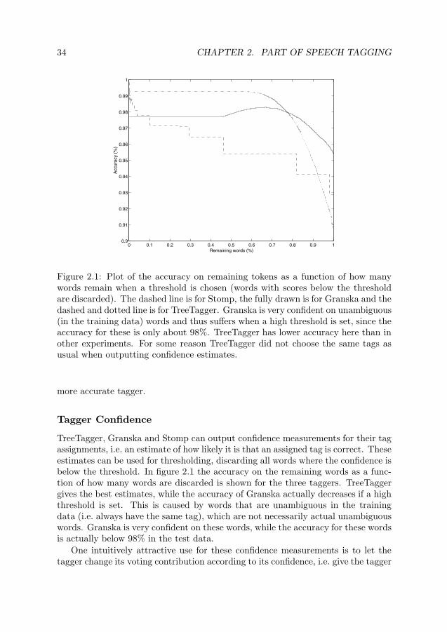
34 CHAPTER 2. PART OF SPEECH TAGGING
0 0.1 0.2 0.3 0.4 0.5 0.6 0.7 0.8 0.9 10.9
0.91
0.92
0.93
0.94
0.95
0.96
0.97
0.98
0.99
1
Remaining words (%)
Acc
urac
y (%
)
Figure 2.1: Plot of the accuracy on remaining tokens as a function of how manywords remain when a threshold is chosen (words with scores below the thresholdare discarded). The dashed line is for Stomp, the fully drawn is for Granska and thedashed and dotted line is for TreeTagger. Granska is very confident on unambiguous(in the training data) words and thus suffers when a high threshold is set, since theaccuracy for these is only about 98%. TreeTagger has lower accuracy here than inother experiments. For some reason TreeTagger did not choose the same tags asusual when outputting confidence estimates.
more accurate tagger.
Tagger Confidence
TreeTagger, Granska and Stomp can output confidence measurements for their tagassignments, i.e. an estimate of how likely it is that an assigned tag is correct. Theseestimates can be used for thresholding, discarding all words where the confidence isbelow the threshold. In figure 2.1 the accuracy on the remaining words as a func-tion of how many words are discarded is shown for the three taggers. TreeTaggergives the best estimates, while the accuracy of Granska actually decreases if a highthreshold is set. This is caused by words that are unambiguous in the trainingdata (i.e. always have the same tag), which are not necessarily actual unambiguouswords. Granska is very confident on these words, while the accuracy for these wordsis actually below 98% in the test data.
One intuitively attractive use for these confidence measurements is to let thetagger change its voting contribution according to its confidence, i.e. give the tagger

2.3. COMBINING TAGGERS FOR BETTER RESULTS 35
more weight for words where it is confident. This was tried in several ways. Firstby letting a tagger overrule the voting when confidence is above a chosen threshold,otherwise voting as normal. Second, by ignoring the vote from a tagger whenthe confidence is below a chosen threshold. Finally, by giving the tagger a voteproportional to the confidence. This was tried for all three of the taggers above,both one at a time and all at once.
Unfortunately, this does not improve on simple voting (though the accuracyis not significantly worse either), despite the fact that for instance TreeTaggerhas an accuracy above 99% for some thresholds (or below 40% when ignoring lowconfidence words). This is caused by the fact that in general the different taggersfind the same words hard (or easy) to tag. For words where TreeTagger achieveover 99% accuracy most of the other taggers also achieve about 99% accuracy. Thismeans that they can correct each other in the few cases one of them is wrong, sovoting is still superior.
The only exception to this is Stomp, which measures its confidence based onhow many words of matching context it found in the training data, which whenusing a high enough threshold actually improves voting slightly. This is probablybecause it does not use the same type of information that most other taggers do(i.e. n-grams of tags), and thus does not always find the same words hard (or easy)as the other taggers. Unfortunately matches where Stomp is confident are veryrare, so the increase in accuracy is very small.
Of course, the opposite is also true, words most of the taggers find easy arenot always tagged very well by Stomp. This is less useful since the other taggersgenerally agree on the correct tag already.
Though tagger confidence did not help while voting, since most taggers foundthe same words easy or hard, the estimates could be used for other things. Oneexample is detecting possible errors in an existing tagged corpus. When the tag inthe corpus differs from the suggested tag and the confidence of the tagger is highenough there is probably an error in the corpus.
They could also be used in creating a new tagged corpus quickly, as manuallychecking only (the few) tags with low confidence would still catch most taggingerrors. Using this kind of information for choosing when to trust the tagger hasbeen examined before, for instance by Elworthy (1994).
Stacked Classifiers
Another way to combine the taggers in an ensemble is to train a new classifier onthe tags selected by the taggers. This has the potential to correct even those caseswhere none of the taggers choose the correct tag (which no voting scheme coulddo). For 1.2% of all words in these experiments, no tagger is correct. It is alsoeasy to combine taggers that use different tag sets in this way, while voting is muchtrickier if not all taggers use the same tag set.
For the evaluation of the stacked classifier approach, some extra work was done.First, all the taggers were trained on a training set and each then tagged an inter-

36 CHAPTER 2. PART OF SPEECH TAGGING
Tagger Accuracy (all words)
Best tagger 96.0Timbl 96.7Relief-F 96.8
Table 2.8: Accuracy of two new second level classifiers and the best single tagger.The new classifiers were trained on the output of the PoS taggers (and, in the caseof Timbl, the tag of the next word). Relief-F was trained and tested on very fewexamples.
mediary set. This intermediary set did not overlap the training set. This was thenrepeated for other choices of intermediary and training set, while keeping all inter-mediary sets disjoint. The intermediary sets were then combined into one dataset,consisting of 580,000 words, and the stacked classifiers were evaluated by 10-foldvalidation on this dataset.
Training Timbl, as a memory based learner, on the output of several taggers(Granska, Mxpost, Stomp and TnT) gives 96.6% accuracy. Adding other typesof information, such as the estimated probabilities of Granska and TreeTagger,decreases accuracy. This is because the method used by Timbl cannot detect thattwo features are dependent (e.g. use the tag TreeTagger suggests only if TreeTaggeris confident). Using context increases accuracy slightly, training Timbl on the tagsfrom fnTBL, Granska, Mxpost, Stomp, TnT and the tag selected by voting on thefollowing word gives 96.7% accuracy.
Another stacked classifier was created using the Relief-F algorithm (Kononenko,1994) to estimate which attributes to use when building a decision tree. Relief-F iscapable of finding codependent features. It was given the following input: the tagschosen by Granska, Mxpost, TreeTagger, Stomp, TnT, Timbl (as tagger), and theconfidence estimates of Granska, TreeTagger and Stomp. It achieves high accuracy,96.8%, but this was tested on a small data set (9,000 words training data, 1,000words test data, 10-fold validation), since Relief-F is very time consuming (weeksor months) with larger data sets.
Another way of using a stacked classifier is to specialize it on words which arebelieved to be hard. One way to do this is to consider tags for which all taggersagree as “good enough” and the other words as hard. This will hopefully allow thestacked classifier to learn what to do for the words were voting is less successful.This reduces the problem the stacked classifier has to learn, but it also reduces theamount of available training data.
This was tried by training and testing Timbl only on those tags where therewere at least two suggestions from the tagger ensemble (using 10-fold validation).Accuracy on these words was then around 78%, which gives a total accuracy of96.6% (these word make up about 11% of all words and the accuracy on the rest is99%). This is the same accuracy as when using Timbl as a stacked classifier on all

2.3. COMBINING TAGGERS FOR BETTER RESULTS 37
words, so there was no improvement over a regular stacked classifier.
Error Analysis
Generally, errors occur in a “mirror” patter, i.e. if words with tag X are oftenmisstagged as Y, then errors of misstagging type Y words as X will also be com-mon. The most common type of tagging errors made by the taggers are choosingsingular instead of plural and vice versa for nouns (7% of all errors), adjective vs.adverb (10%), determiner vs. pronoun (7%), proper noun vs. noun (7%), particlevs. adverb (5%), preposition vs. particle (4%). This corresponds well to otherexaminations of Swedish PoS tagging (Megyesi, 2001).
After voting there are still many errors of these types. The number of errors ofsome of these types actually increases. One example is the singular/plural problemfor nouns. Before voting 7% of the errors belonged to this type. The number ofsuch errors after voting would correspond to 8% of the original errors, and makeup 10% of all errors that remain after voting. Before voting there are about 1,200different error types, after voting there are only 900 types. This means that mostlyuncommon errors are corrected, and that the errors that remain are concentratedto fewer categories. This is an interesting property, since it is less work to writemanual correction rules for the (few) common error types than for the (many)uncommon error types.
The stacked classifiers behave similarly to voting, they mainly correct uncom-mon errors.
A small test shows that it is possible to write rules that correct some of thetagging errors. These rules can for instance make use of longer scope or semanticclues that the taggers cannot use. Four rules were created (by a non-linguist) ina few hours and applied on the tags selected by voting. These rules corrected 131errors and introduced 32 new errors (and one error was changed to another error)for a net gain of 99 correct tags.
While it is possible to write rules to correct some tagging errors it seems hard toget large improvements, though using a trained linguist or more time to constructrules might achieve better results. One problem is that the common errors aremistaking one common tag for another common tag, so rules trying to correct thisoften introduce many new errors because there are so many correctly assigned tagsof these types.
Many of the remaining errors are actually errors in the corpus, ambiguities wherethe suggested tag could also be considered correct or words where the correct tagcan only be selected by semantic knowledge.
See Källgren (1996) for a discussion of common error types for automatic andmanual tagging in SUC.

38 CHAPTER 2. PART OF SPEECH TAGGING
2.4 The Lexicon for the Tagger
Here, factors that are important regarding the training data of the tagger are dis-cussed. The original problem was that we wanted to make a tagger we had, herecalled Granska, see section 1.2, freely available. The tagger is however not veryuseful without its lexicon, here used to mean the data collected from the annotatedtraining data. The lexicon we had was not freely available, though we had a licenseto use it ourselves. It turned out that it is possible to create a new free lexicon byautomatic means, and if you do it right the tagger using this lexicon outperformsthe tagger using the original lexicon. Most of this research was presented at ICON2004 (Sjöbergh, 2003a).
The Lexicon
The tagger was developed for written Swedish, but is relatively language inde-pendent and can easily be retrained for many other languages. It is based on HMMusing trigrams of PoS tags. Normally it is automatically trained on the SUC corpusdescribed in section 1.2.
When the tagger creates a lexicon it needs a PoS annotated corpus. Preferablythe lemma of each word should also be provided, and sentence boundaries shouldbe marked. The tagger has a lemma guesser and a sentence boundary detectionmechanism, so only part of speech information is strictly necessary. Also, the lemmainformation is not used much in actual tagging (but for some unknown words itcan be used), but mostly for guessing lemmas of new text (which in turn is usedby the grammar checking framework the tagger is normally used in).
From the annotated training data the following information is extracted:
• Word frequencies. Word-tag pair frequencies and word-tag-lemma triple fre-quencies.
• Tag n-grams. Unigram, bigram and trigram frequencies.
• Suffix information. All suffixes of lengths between two and five letters, fromwords in any open word class are collected, as suffix-tag pair frequencies.
This data is what is referred to as a “lexicon” in this section. The tag n-gramsand the word-tag frequencies are used when tagging known words, while the tagn-grams and the suffix information is used when tagging unknown words. Forunknown words, other factors like capitalization are also used.
Creating a New Lexicon
The basic idea in creating a new lexicon was to take freely available unannotatedtexts and automatically annotate these, then train the tagger on the newly annot-ated data. The texts were taken mainly from the KTH News Corpus, described insection 1.2.
2.4. THE LEXICON FOR THE TAGGER 39
Several freely available taggers were collected. The taggers used were the sameones used in the previous section on combining taggers for better accuracy:
• fnTBL, see section 1.2, a transformation based tagger.
• Granska, see section 1.2, a trigram HMM-tagger.
• Mxpost (Ratnaparkhi, 1996), a maximum entropy tagger.
• Stomp, described in detail in section 2.2.
• TnT, see section 1.2, a trigram HMM-tagger.
• TreeTagger (Schmid, 1994), a tagger using decision trees.
These were automatically trained on the SUC, using default options as far aspossible. When trained, the taggers all tagged the new texts from the KTH NewsCorpus. The results were combined by simple voting, giving each tagger one voteand picking the tag which received the most votes. Ties were broken by a prede-termined tagger. Though there were methods that achieved better accuracy thansimple voting in the previous section, voting was almost as good and is very easy toimplement, especially in our case since all taggers were using the same tag set. Inthe spirit of avoiding work as much as possible, voting was deemed good enough.
After annotating the new data with part of speech tags, the Granska tagger wasrun on the tagged text, in lemma guessing mode, to add lemma information andsentence boundaries.
The Granska tagger, which the new lexicon is to be used by, was then trainedon the new data. The quality of the lexicon was evaluated on a test set from SUC,consisting of 60,000 words and disjoint from the part of SUC used when training thetaggers. The test set was tagged with the Granska tagger using different lexiconsand the quality of the lexicons compared by comparing the accuracies on the testset.
This method of creating a new lexicon requires very little manual labor, onlyacquiring the taggers and the texts, and then starting the training and tagging(which is then automatic).
Evaluation of Lexicons
A few variations where tried when creating the new training data, to see what effectdifferent methods have on the resulting lexicon. The following expected behaviorswere evaluated: the more training data used, the better the lexicon; using severalgenres is better than using only one (e.g. newspaper texts); using well written textsis better than using texts with many errors; using many taggers to annotate thenew texts is better than using only one.
This was evaluated by using the following strategies for annotating the trainingdata:

40 CHAPTER 2. PART OF SPEECH TAGGING
• Using only the tagger itself when tagging the training data.
• Using the voting ensemble when tagging the training data.
• Using only sentences where all taggers agree on the tagging as training data.This gives less training data (about 90% of the data is discarded) but thetagging accuracy on the remaining data is very high.
To test some of the assumptions above, other texts were added to the KTHNews Corpus texts (but some of these can likely not be included if the lexicon is tobe freely available). The following are examples of variations of the training data:
• Adding other genres, in this case text from an encyclopedia.
• Adding malformed language, in the form of essays written by second languagelearners, to the training data (to see if the quality of the texts is important).
• Adding text of high quality but which is not modern Swedish, in the form ofa novel from 1879.
The performance of the tagger using lexicons constructed by these methods canbe found in figures 2.2 and 2.3. In figure 2.4 a comparison of how much manuallycorrected data is needed to achieve a certain accuracy level is shown, by usingdifferent amounts of data from the SUC.
As expected the new lexicon gives worse performance than the one createdfrom the manually corrected SUC. This is because the taggers strengthen theirmisconceptions from the original training data on the new texts. The best accuracyachieved (when using all available data, 10 million tokens of newspaper texts, 3million tokens of encyclopedia text, 100,000 tokens of student essays and 100,000tokens from a novel) was 95.6% and the best accuracy when using only the KTHNews Corpus texts was 95.3%. The accuracy when using the manually correctedSUC was 96.0%. To achieve the same accuracy as the best result of the automaticmethod using manually corrected annotation would require roughly 700,000 tokensof annotated text, if the new texts are from the same (balanced) domain as the testdata. This can be seen in figure 2.4, where different amounts of training data fromthe SUC were evaluated.
The more data used for training, the less the degradation in tagging accuracywith the new lexicon. While adding more training data improves the lexicon, therate of improvement decreases when the training set becomes large.
Annotation Methods
As can be seen in figure 2.2, using an ensemble of taggers when annotating the newtraining data gives better performance than using the tagger alone. This is becausethe taggers correct each other, so the annotation of the training data contains fewererrors than when using only one tagger. The best result using the ensemble on the

2.4. THE LEXICON FOR THE TAGGER 41
0 1 2 3 4 5 6 7 8 9 10
x 106
0.93
0.935
0.94
0.945
0.95
0.955
0.96
0.965
training data size (tokens)
accu
racy
(%
)
Figure 2.2: Tagging accuracy when using different lexicons, as a function of thesize of the training data used when creating the lexicon. The dashed line is theaccuracy when using the manually corrected SUC as training data and the dottedline is when using all available new data.x using only the tagger itself to tag the training datao using an ensemble of taggers* using only the sentences where all taggers agree on the tagging.
newspaper texts was 95.3% and the best result on the same texts using only thebest single tagger alone was 95.1%.
For words where all the taggers in the ensemble agree on the tagging, the taggingaccuracy is very high, above 99%. To see if using only such data is a good ideaa training set was created by using only those sentences where all taggers agreedon the tagging of all words. This results in much less training data, about 90% ofthe data is discarded, but with less tagging errors in the remaining data. This didnot improve the lexicon, even when compared to a lexicon created from an equalamount of training data tagged by voting. In fact, it is even worse than using onlyone tagger. The highest accuracy when using only data where all taggers agree was94.0%, and the accuracy when using the same amount of data (though of coursenot the same sentences) was 94.2% when tagged by one tagger and 94.4% whenusing the ensemble.
One reason for the perhaps surprisingly bad performance when using only thehighly accurately annotated sentences, is that the data consist mostly of simpleconstructions. The difficult constructions are not represented at all in the training

42 CHAPTER 2. PART OF SPEECH TAGGING
0 1 2 3 4 5 6 7 8 9 10
x 106
0.935
0.94
0.945
0.95
0.955
0.96
0.965
training data size (tokens)
accu
racy
(%
)
Figure 2.3: Tagging accuracy when using different lexicons, as a function of the sizeof the training data used when creating the lexicon. The dashed and dotted linesare the same as in figure 2.2.o using only newspaper texts+ using only encyclopedia textsx using newspaper texts and some malformed text (second language learner studentessays)* using both encyclopedia and newspaper textsIn all cases the ensemble of taggers tagged the text.
data, since some tagger usually makes a mistake on the difficult constructions. Thismeans that the tagger only learns how to tag simple language constructions, whilethe test data (and most real texts) contain difficult constructions too, which thetagger cannot handle well without seeing them in the training data.
Genres
Since different text genres have somewhat different characteristics, using only onegenre (in this case newspaper texts) when training was expected to be worse thanusing several genres, since the test data consists of balanced material, not justnewspaper texts. To test this, texts from an encyclopedia, the Nationalencyklo-pedin (NE, 2000), were tagged in the same way as the newspaper texts. Thesetexts consisted of about 3 million tokens. The performance of lexicons createdfrom only newspaper texts, only encyclopedia texts and from a mix of both wasthen evaluated. The results are shown in figure 2.3.

2.4. THE LEXICON FOR THE TAGGER 43
0 2 4 6 8 10 12
x 105
0.915
0.92
0.925
0.93
0.935
0.94
0.945
0.95
0.955
0.96
0.965
training data size (tokens)
accu
racy
(%
)
Figure 2.4: Tagging accuracy when using different lexicons, as a function of the sizeof the training data used when creating the lexicon. The training data is the SUC,a manually corrected, balanced corpus of Swedish text. The dashed and dottedlines are the same as in figure 2.2.
As expected, using texts from both genres gave much better results than usingonly one genre. Using only encyclopedia texts was roughly as good as using onlynewspaper texts, though when using small amounts of text, the encyclopedia textswere worse, likely caused by selecting only the first part of the encyclopedia andthus getting a skewed distribution (i.e. too many words starting with the letter“a”). Using only newspaper texts the best accuracy was 95.3% and for the sameamount of training data using both encyclopedia and newspaper texts, the accuracywas 95.5%.
Text Quality
To see if the quality of the texts is important, 100,000 words from second languagelearner essays were added to the training data. These texts contain many erroneousconstructions and misspelled words. Somewhat unexpectedly, adding malformedlanguage to the training data improved the lexicon when compared to a lexiconcreated from an equal amount of data consisting only of newspaper texts. This isprobably caused by the addition of new genres to the training data, which as seenearlier is good, even when some of the new material is ungrammatical. Replacingthe essays with the novel “Röda rummet” (“The Red Room”), Strindberg (1879),which consists of well written nineteenth century Swedish (i.e. not modern Swedish),gave the same accuracy, while replacing it with an equal amount of encyclopedia

44 CHAPTER 2. PART OF SPEECH TAGGING
text (very high quality text), gave even higher accuracy. This indicates that whilehigh quality text is better than low quality, the benefits of using several genres isgreater than the drawbacks of errors in the text, and that using the same genres inthe training data as in the test/application domain is better than other genres (i.e.in this case modern Swedish of the encyclopedia vs. Strindberg).
Some reasons for text quality not being very important can be seen from theproperties of the tagger. The errors in the essays consist of spelling errors, whichdo not affect the tagger, and grammatical errors, which do affect the tagger. Thereason spelling errors do not affect the tagger is that they will contribute a lot ofmisspelled words to the lexicon, but these will have no effect on the tagging of otherwords, unless the new words are the same misspelled words. Theoretically, spellingerrors could possibly help the tagger, by having the ensemble guessing the tag andthereby having more input on how to tag unknown words (most misspelled wordswill be uncommon and thus used in training the taggers behavior on “unknown”words, so there will be more words for “unknown” word training). Also, the trainingdata only needs to be locally (grammatically) correct to be useful, and many localconstructions are correct in the essays.
Combining Automatic and Manual Annotation
Finally, to combine the usefulness of large amounts of data with the usefulnessof high quality annotation (i.e. manually annotated data), both the KTH NewsCorpus annotated by the voting ensemble and the manually annotated SUC wasused as training data. The lexicon produced using this training data was betterthan using only the manually annotated data, resulting in a slight improvement,96.2% accuracy. Using the SUC and data automatically annotated only by theGranska tagger itself was less accurate than only using the SUC, the tagger tendsto reinforce its misconceptions.
2.5 Important Points
In this chapter it was shown that combining several methods for PoS tagging is asimple way to improve the tagging quality. Many machine learning implementationsare readily available, thus better results can be achieved with no extra manual work.
Using extra information from the systems, such as estimates of how reliable thecurrent guess is, generally gave very modest improvements. Possibly, better resultscould be achieved with larger data sets, since there is something of a sparse dataproblem when adding the extra dimension of system confidence.
When combining learning systems, it would be best if they made independenterrors. This will rarely if ever happen in this type of application, but using systemsthat are as different as possible is good, even if the individual systems are not thataccurate.
Similar things can be said for the training data: having many different genresis good. Adding text with low text quality is still good, at least if this widens the

2.5. IMPORTANT POINTS 45
genre coverage. With regards to training data, it was also shown that combininga relatively small amount of high quality (i.e. manual) annotation with very largeamounts of automatically annotated data gave better results than either source byitself.


Chapter 3
Compound Splitting
3.1 Introduction to Compound Splitting
Swedish is a compounding language, and compounding is very productive. So inSwedish a “glass bowl” would be written as the word “glas” (meaning “glass”)and the word “skål” (“bowl”) written together, “glasskål” (“glass bowl”). Com-pound words can be made using many words, not just two, though most compoundscontain only two or three components.
In NLP Applications it is often useful to split compounds. It can for instancehelp in finding more relevant pages when using a search engine (Dalianis, 2005),improve clustering (Rosell, 2003), make hyphenation more readable by hyphenatingat the correct compound component borders or be used in machine translation,where most likely not all compounds will be listed in the translation lexicon, butmost compound components could be included.
Many compound words have more than one possible interpretation, such as“glas-skål” (“glass bowl”) and “glass-skål” (“bowl of ice cream”), both of whichare written as “glasskål”. In most cases a human reader will have no problem todetermine the correct interpretation of a word in context, while this is much harderfor automatic methods. Automatic methods also have problems with interpreta-tions that are clearly very unlikely, such as “glass-kål” (“ice cream cabbage”).
The easiest and most common way of splitting compounds is to simply havea lexicon where the correct interpretation of each compound is listed. This ofcourse does not solve the problem of genuinely ambiguous compounds, and alsosuffers from the fact that there will always be compounds that are not listed in thelexicon, usually quite many, since compounding is so productive.
Other methods that have been tried include studying letter sequences that canonly occur on the border of two compound components, never in a non-compoundword. For Swedish, “kk” and “stp” would be examples of such letter sequences. Ofcourse, most compound borders do not contain such letter sequences, so this onlyhandles a limited number of compounds.
47

48 CHAPTER 3. COMPOUND SPLITTING
For Swedish, both rule based methods (Karlsson, 1992, Dura, 1998) and stat-istical methods (Kokkinakis and Johansson Kokkinakis, 1999, Sjöbergh and Kann,2004) have been used for automatic compound splitting. Similar research has beendone for other languages, such as German (Koehn and Knight, 2003), Norwegian(Johannessen and Hauglin, 1996) and Korean (Yoon, 2000).
The research presented here was done together with Viggo Kann, and parts ofit has been presented at LREC 2004 (Sjöbergh and Kann, 2004) and in the journalSpråk och Stil (Sjöbergh and Kann, 2006). The main focus is on using statisticalmethods for selecting the correct interpretation from several suggestions, but amethod for finding the possible interpretations is also presented.
3.2 How to Find Possible Interpretations
The spelling error detection program Stava, described in section 1.2 was modified tofind all possible splittings of compounds. Unlike Stava, where the algorithm stopsthe search when a possible splitting of the word is found, the algorithm used insteadproceeds to find all possible interpretations of the compound. The algorithm is quitefast, finding all possible interpretations of more than 60,000 words per second on astandard computer.
3.3 How to Select the Correct Interpretation
In this section several statistical methods to choose the correct interpretation, fromseveral possible interpretations, of Swedish compounds are presented. These meth-ods are generally not very closely tied to Swedish, so they should work for manyother languages too. A summary of how well the different methods work can befound in table 3.1.
Evaluation Method
In a text of 50,000 words taken from the SUC corpus described in section 1.2, allcompound words with at least one suggestion from the program finding interpreta-tions were manually annotated with their correct interpretations. 3,400 words hadat least one suggestion, 1,200 words had more than one suggest interpretation. Ifnothing else is specified, all accuracy figures are based on the 1,200 words that arein this way ambiguous.
Some compound words in the text had no suggestion at all from the program. Amanually checked sample showed that less than 1% of the compounds were missedin this way. The biggest problem is compounds containing proper names, such as“Venusmålningarna” (“the paintings of Venus”) and “Hitchcockläroboken” (“thereading material on Hitchcock”). Generally, there are not very many proper namesin the first part list, so these words will not be split. This can of course easily bemitigated by adding common proper names to the list.

3.3. HOW TO SELECT THE CORRECT INTERPRETATION 49
For 99% of the 2,200 compounds that had only one suggestion, this suggestionwas the correct one. For 99% of the 1,200 compounds with several suggestions, oneof the suggestions was the correct interpretation. Here too, most of the problematic1% were caused by proper names, giving “Ko-rea-kriget” (“the war over selling cowscheaply”) instead of “Korea-kriget” (“the Korean war”).
Many words that are not compounds can also be split by the program, such as“vita/vi-ta” (“white/we + take”), “James/Ja-mes” (“James/Yes + small bird”).This has been avoided by never splitting words that can occur as a non-compoundword, i.e. words that are listed in the last part list or individual word list. Of course,some non-compound words are still analyzed as compounds, especially inflectedforms, but it is rare. In the test data, 18 words that are not compounds were stillsplit. Such words were ignored in the evaluations. Some words that could alsobe seen as compounds, mainly Swedish family names, which are often made up bytaking two words and writing them together, were also ignored. These were deemedless interesting to include in the study. They tend to be easy but almost alwaysuninteresting to split. In the test data, all such words had only one suggestedinterpretation.
The program for generating suggestions has a coverage of 99%, in the sense that99% of all compounds in the test data have a set of interpretations suggested thatinclude the correct interpretation. It also has a precision of 99% in the sense thatfor all words that have interpretations suggested, at least one of these is the correctinterpretation. Words that are not compounds are included here, but can of coursenever have a correct suggestion.
Systems for analyzing Swedish compounds have been created before. The mostfamous is probably SWETWOL (Karlsson, 1992), based on manually written rulesusing the two level formalism. Just like the program used for generating suggestionsto choose from, SWETWOL produces all the interpretations it can find.
SWETWOL can handle some words that the Stava based program does nothandle, such as “Venusmålningarna” (“the paintings of Venus”). Naturally, thereare still many words that it cannot handle, such as “Hitchcockläroboken” (“thereading material on Hitchcock”). Some words that the Stava based program handlesare not handled by SWETWOL. On the 3,400 compounds included in the test data,94% had the correct interpretation among the suggestions from SWETWOL.
When the correct interpretation was not available, it was generally causedby the word not being analyzed as a compound word. Examples of words nothandled correctly by SWETWOL include “yngel|boet” (“the nest of the young-lings”), “guda|borgen” (“the castle of the gods”), “nikotin|gula” (“nicotine yel-low”), “läsvane” (“having a large experience of reading”) and “åskblå” (“thunderblue”).
This means that SWETWOL has higher precision, basically 100%, but lowerrecall than the Stava based program.

50 CHAPTER 3. COMPOUND SPLITTING
Baseline, the Number of Components
One simple way of choosing an interpretation is to take the one with as few com-ponents as possible. “Korea-kriget” (“the Korean war”) would be preferred to“Ko-rea-kriget” (“the war over selling cows cheaply”), since it has only two com-ponents compared to three. This is motivated by the fact that compounds with twocomponents are much more common than compounds with three, which in turn aremuch more common than those with four etc.
If several suggestions have the same number of components, the one that hasthe longest last part is selected, since it is more common with inflectional endingsmaking the last part long than with short components in compounds. “Upp-rättar”(“establishes”) would be preferred to “upprätt-ar” (“upright area”).
This simple and very fast method works quite well and handles 93% of theambiguous compounds in the test corpus correctly.
Words in the Context
Compounds with several reasonable interpretations of course require the use of in-formation from the context to find the correct interpretation of a certain occurrence.This type of ambiguity is quite rare, but using contextual information can be usefulin other cases too. A simple way to use the context of a compound is to check if anyof the compound components occur as free words or parts of other compounds inthe near context. In a sentence mentioning a famous glass blower (“glas-blåsare”),“glas-skål” (“glass bowl”) seems more likely than “glass-skål” (“ice cream bowl”),since the “glas” (“glas”) component occurs in the same sentence, but the “glass”(“ice cream”) component does not.
With this in mind, the following method was implemented: For each suggestedinterpretation the occurrences of its components as either a word or a part ofa compound word in the context were counted. A context window of fifty wordsbefore and fifty words after the compound was used. The occurrences were weightedby the distance to the compound, so that closer words were given higher weight.The interpretation with the highest mean value of its components was selected.
This method works poorly, giving the correct interpretation in only 75% of thecases. This is caused by data sparseness. A compound component rarely occurs inthe context. If stems of words and components are used the results are improvedslightly, though it is sometimes hard to say what the stem of a compound head is.
Another problem with this method is that it is common that erroneous inter-pretations contain many short components, such as “han-del-s-min-ister” (“he-part-s-my-fat”) instead of “handels-minister” (“minister of trade”). Short componentshave a good chance of occurring in the context by chance, since short words tend tobe common words. If all suggestions with more components than the one with thefewest are first removed and the context method is then used as above to choosebetween the remaining suggestions, the method works much better. 94% of thecompounds are then correctly interpreted.

3.3. HOW TO SELECT THE CORRECT INTERPRETATION 51
Human readers of course use more context information than the occurrences ofcompound components. It would probably suffice to know that the general topic ofa text is related to photography to decide that “bild-rulle” (“roll of film”) is morelikely than “bil-drulle” (“bad driver”). This type of knowledge is hard to captureusing automatic methods, but there are methods that try to do this. One suchmethod is Random Indexing, RI (Sahlgren, 2005). RI is described in more detailin section 1.1. In short, it measures how related two words are using co-occurrencestatistics. Words that tend to co-occur with the same words are considered related.
If the method above is modified to calculate the average relatedness of thecomponents and the context words instead of just counting occurrences of the com-ponents, performance is improved to 96%. This is one of the best methods ofthose presented here. As above, it performs poorly if suggestions with many shortcomponents are also allowed. If these suggestions are also kept, only 51% of thecompounds are correctly interpreted. The reasons are also similar, short compon-ents correspond to common words, which are often seen as a little related to manywords.
These context methods have the interesting property that they can choose dif-ferent interpretations for the same compound in different contexts. In our tests, thecontext method using RI was the only method that did select different interpret-ations for the same compound in different parts of the test data, for instance forthe word “kol-atom” (“carbon atom”), which was also interpreted as “kola-tom”(“empty of caramel”). Unfortunately the text was discussing carbon atoms in bothplaces, but it is none the less an interesting property. Most methods presented hereand in other research always choose the same interpretation for the same compound.
Relation Between Components
When a way to measure the relatedness of two words is available, such as the oneused in the previous section, it can also be used to see how related the componentsof a suggested interpretation are to each other. When looking at the word “glasskål”we can ask ourselves how often bowls are made of glass (“glas-skål”, “glass bowl”),how often ice cream is eaten from a bowl (“glass-skål”, “ice cream bowl”) and howoften ice cream and cabbage are eaten together (“glass-kål”, “ice cream cabbage”).
This was tried by calculating the mean relatedness score between the compon-ents of each suggested interpretation, using the RI method to measure relatedness.As in the previous section it works poorly when allowing suggestions with manyshort components, 46%, and works well if these are first removed, 96%.
Component Frequencies
One method to use statistics when interpreting compounds is to choose “glas-skål”(“glass bowl”) over “glass-skål” (“ice cream bowl”) on the basis that compoundswith the word “glas” are more common than compounds with “glass”. Frequencystatistics were collected for compound heads and tails. The suggested interpretation

52 CHAPTER 3. COMPOUND SPLITTING
with the highest geometric mean value of the frequencies of its components wasselected.
This method worked about as well as the baseline method selecting interpreta-tions with few components, 93% correct. Data sparseness is again the main prob-lem. Many components of the suggested interpretations did not occur at all in thetext collections from which the frequency data was collected. Several different textswere tried: the one million words from the SUC corpus (this uses only frequenciesof words, not compound components, since the compounds are not split in this cor-pus); 84,000 compounds from the SAOL word list (SAOL, 1986) (annotated withtheir correct interpretations); the 84,000 compounds from SAOL but with frequen-cies of the compounds taken from the SUC corpus; 300 compound words from SUC,manually annotated with their correct interpretation.
The best results were achieved using the 84,000 compounds with occurrencefrequencies from SUC. Using only the word list gives too much weight to rarewords, using only SUC does not give information on the compound componentlevel and using only 300 compounds gives too little data. The results would likelybe better if frequencies from a large corpus annotated with the interpretations ofcompounds were available.
Of the 84,000 compounds from SAOL, only about 10,000 occur in SUC, with anaverage of four occurrences each for these. About 14% of the compounds occurringin SUC are listed in SAOL. This was manually checked in a small sample.
If the powerful heuristic of discarding suggestions with many components isused, the results are once again improved, giving 95% correctly interpreted com-pounds.
PoS Context
Often it is clear from the context what the PoS of the compound should be. If dif-ferent suggested interpretations have different PoS, this type of context informationcan be used to select the most likely interpretation.
This was tried by using the statistical PoS tagger TnT described in section 1.2,which was also used in the previous sections on PoS tagging.
TnT was used to tag the text, with the compound exchanged for the tail of thesuggested interpretation, since the tail determines the PoS in Swedish. TnT wasalso run on the text with the compound replaced with a dummy word, to make TnTselect the most likely PoS based solely on the context information. All suggestionswith a different PoS was then discarded and the baseline method using the numberof components were used to select an interpretation between the remaining ones.
This method did not work very well, only 87% correct, which was lower thanthe baseline method alone. In most cases all suggestions have the same PoS, soit is rarely applicable. In the cases some suggestions received a different PoS, itwas usually just a tagging error. It was also common that the suggestion thatwas different had a very short component as the tail, which made a favorable

3.3. HOW TO SELECT THE CORRECT INTERPRETATION 53
PoS interpretation possible, since short words are often ambiguous. As mentionedearlier, short components are rarely the correct interpretation.
If as before suggestions with many short components are discarded first, theaccuracy is improved but still not very good, 90%.
PoS of Components
Some word class combinations are much more common in compounds than others.Noun noun compounds make up more than 25% of all compounds for instance,while pronoun pronoun compounds are extremely rare.
To use this information, a PoS tagger for compound components was needed.No such program was available, most likely because this type of information israrely of interest, so a very naive program was created. The program essentiallyjust makes a lexicon lookup to find the possible PoS of a component. No use ofcontext information is made. For heads of compounds, which often undergo slightmorphological changes, a few simple morphological rules are used if no lexiconentry is found. No disambiguation is performed, all interpretations are kept. Theprogram is not very accurate, especially the heads are often incorrectly tagged.This is not a great problem though, as explained below.
For each suggested interpretation the probability of the head and tail PoS com-bination was calculated. If there were several available PoS for either head or tail,the most favorable interpretation was used. If there were more than two compon-ents, the probability for each head PoS occurring with the tail PoS was calculatedand the total probability was calculated as the product of these. The suggestionwith the highest probability was chosen as the correct interpretation.
The probabilities for head and tail PoS combinations were automatically calcu-lated by using the tagging program above to annotate the PoS of the componentsof 300 compounds manually annotated with their correct interpretations. Since theproblem consistently makes the same types of mistakes on this reference data ason the new data, the somewhat low accuracy of the program is not a very seriousproblem. It would likely be better if the program was more accurate, though. Itwould likely also be better if the reference data was considerably larger. Despitethis, the method works well, with 94% accuracy.
Letter n-grams
Some letter sequences never occur in non-compound words in Swedish, examplesinclude “kk” and “stp”. When these are found in a word, there must be a compoundborder at least in this place. This property has been used to split compoundwords (Kokkinakis and Johansson Kokkinakis, 1999). Most compound words donot contain such letter sequences though.
Similar information can also be used to choose between different suggested in-terpretations. Even when the letter sequences across the compound border canoccur in non-compound words, they are often rare in non-compounds.

54 CHAPTER 3. COMPOUND SPLITTING
To use this information, frequencies of letter 4-grams from compound headsand compound tails were collected. 4-grams spanning a compound border werenot counted. The frequencies were collected from the 84,000 compounds in SAOL,weighted with frequencies from SUC.
For each suggested interpretation, the sum of the frequencies of all 4-gramsspanning the suggested compound borders was calculated. The suggestion withthe lowest sum was then selected. This was thus the suggestion with the lettersequences least likely to occur where there is no compound border.
As an example, consider the word “genomarbetat”, which has two possibleinterpretations from the first analysis step: “gen-omarbetat” (“genetically redone”)and “genom-arbetat” (“thoroughly gone through”). The first suggestion has thefollowing 4-grams and frequencies: “geno (339)”, “enom (342)” and “noma (4)”,sum 685. The second suggestion has: “noma (4)”, “omar (4)” and “marb (14)”,sum 22. Suggestion number two, “genom-arbetat”, is thus selected, since it putsthe compound border at the very rare (in non-compounds) “marb” and “omar”,instead of the word internally more common “enom” and “geno”.
Of the 18,959 4-grams in the compounds in SAOL, 10,211 occur at least fivetimes in SAOL. If instead the frequencies are calculated with weights from SUC,only 3680 4-grams occur at least five times. Only 7634 of the 4-grams occur at allin SUC. The cause is the previously mentioned fact that only a small part of thecompounds from SAOL occur in SUC and only a small part of the compounds inSUC are listed in SAOL).
Using letter 4-grams worked well, with 95% accuracy. Shorter or longer n-gramscould of course also be used, or combinations of different lengths. Only 4-gramswere examined though.
Ad Hoc Rules
There are some difficult cases that many of the previously mentioned methodsmake many mistakes on. To handle such cases a couple of ad hoc rules werecreated. One rule handles common inflectional suffixes that can also be interpretedas compound tails. One such example is “or”, a common noun plural suffix thatcan also be interpreted as a rare word meaning a kind of small insect. The firstad hoc rule simply lists a few such words and suggestions with these as compoundtails are discarded. Though there can certainly be cases were the interpretation as acompound component is the correct one, such as “glödhet” (“red-hot”), these casesare rare compared to the suffix interpretations, such as “godhet” (“goodness”), andthey are often suggested as a possible interpretation.
In Swedish, if joining the head and tail results in three identical consonants ina row, the resulting word is written with only two consonants, i.e. “topp” (“top”)and “politiker” (“politician”) would make the compound “toppolitiker” (“top politi-cian”), not “topppolitiker”. This can lead to ambiguities, often with one interpret-ation being much more likely than the other, such as “vin-nyheter” (“news about

3.3. HOW TO SELECT THE CORRECT INTERPRETATION 55
Method Correct (%) Incorrect (%)
Number of components 93 7Words in context 75 25Words in context, few components 94 6Words in context, RI 51 49Words in context, RI, few components 96 4RI between components 46 54RI between components, few components 96 4Component frequencies 93 7Component frequencies, few components 95 5PoS context 87 13PoS context, few components 90 10PoS of components 94 6Letter n-grams 95 5Combination method 98 2
Table 3.1: Correctly analyzed compound words, of those with more than one sug-gestion.
wine”) versus “vinn-nyheter” (“news about winning”). Two reasonable interpreta-tions is also a possibility, as with the previously mentioned “glasskål”.
Many methods have problems dealing with this kind of ambiguity. One sugges-tion has a longer compound tail, one suggestion has letter 4-grams with frequencyzero at the compound border etc. but the reason is not the one the method wasmeant to deal with. Since many methods do not handle this type of ambiguity in anintelligent way, an ad hoc rule choosing the slightly more common two consonantinterpretation was created. Some methods, such as the context methods, do notneed this rule, since they handle this type of ambiguity quite well.
Combination Methods
Since the different methods make slightly different kinds of errors they can becombined and made to correct each other. Almost all compound words have thecorrect interpretation selected by at least one method. A simple way to combinemethods is to let them vote on which interpretation should be selected.
A slightly more complicated combination method was tested. The first step isto discard all suggestions except those with the fewest number of compound com-ponents. For selecting among the remaining suggestions, the method using thecomponent frequencies was used together with the method using the PoS of thecompound components. These methods gave a confidence measure for each sug-gestion and these were combined with slightly more weight given to the frequencymethod. The suggestion with the highest total confidence was selected.
56 CHAPTER 3. COMPOUND SPLITTING
This combination method is correct for almost 98% of the ambiguous compoundsin the test data, which corresponds to slightly more than 98% of all compounds.This is better than either method on its own.
Error Analysis
The errors made by the automatic methods can be divided into four types. Per-centages below are for the combination method in the previous section, but shouldbe considered a bit unreliable, since it only makes 27 errors in our test data. Othermethods make the same types of errors, though in slightly different proportions.
The first error type is to divide a compound at all the correct borders butalso suggest a compound border in at least one more position. One example is“Vig-gen-plan” (“nimble genetic airplane”), where “Viggen-plan” (“Viggen classairplane”) would be the correct interpretation. This type of error is usually causedby the correct interpretation not being available. Since most methods have a verystrong bias towards suggestions with few components, the correct suggestion wouldotherwise be selected. About 20% of the errors were of this type.
Error type number two is similar to the first one. The compound is interpretedas split only at compound borders, but some suggested components are still com-pounds and should also be split. Example: “fotboll-s-lag” instead of “fot-boll-s-lag”(“soccer team”). This is the most common error type with slightly more than 40%of the errors. It can be mitigated by removing compound words from the head andtail lists of the program that generates suggestions.
How much the compounds should be split depends on the application they areto be used for, so this error type is not always bad. When searching for goodhyphenation possibilities, likely all possible compound borders are of interest andthus these errors could lead to less than ideal results. When using compoundsplitting for machine translation it is probably better to keep as long components aspossible, as long as they are words that are included in the translation dictionaries.It is easy to tune how much the compounds should be split by simply varying thecontents of the head and tail lists of the program that generates suggestions.
The third error type is the three identical consonants in a row special case. Thisis a quite hard problem and many of these cases lead to errors. Since this type ofambiguity is not very common though, less than 20% of the errors belong to thistype.
Finally, the fourth error type is when a compound is simply split at the wrongpositions. About 20% of the errors belonged to this type.
3.4 Important Points
In this chapter, methods for automatic compound splitting for Swedish were presen-ted that using quite modest resources achieved good results. 99% of the compoundsin the evaluation texts were split in some way and 98% of them were split correctly.

3.4. IMPORTANT POINTS 57
A large part of the remaining errors belong to a type that is often not a seriousproblem.
The presented methods are based on statistics. This means that there is noneed for explicitly writing rules for the properties of Swedish compounds. Thus,it would likely be simple to apply these methods to other languages, and similarmethods have been used on other languages. Most methods are also very easy toimplement.
Several methods require different types of resources to collect statistics from,though. With the relatively modest resources used here good results were achieved.With larger resources even better results would likely be achieved.
Some compounds require the use of contextual information to be correctly in-terpreted. Compounds of this type are very rare, though. Two methods that usecontext information were presented, one of which worked quite well.
A very simple and powerful heuristic is to discard suggested interpretations withmany compound components. There are however some words that have two reas-onable interpretations with different number of components, for example “matris”(“matrix”) or “mat-ris” (“rice for eating”) and “finskor” (“women from Finland”)or “fin-skor” (“dress up shoes”). Using the heuristic of few compound componentswould thus always make mistakes on one of these interpretations. For this typeof words it is necessary to use context information. Unfortunately, the contextmethods worked poorly without the few components heuristic.
In some applications, such as machine translation, it would be interesting to havethe lemma form of the compound components. This has not been dealt with herebut could be done in a straightforward way by simply adding the lemma informationto the compound component entries in the dictionaries used by the modified Stava.It can be noted though that some compounds have the same component lemmasdespite the compounds being different, such as “broderskap” and “brödraskap”.For some compounds the lemma form is ambiguous, such as “vaknatt” (“nightwatch”), which could be made from “vaka” (“to stay up”) and “natt” (“night”) or“vak” (“wake”) and “natt”.


Chapter 4
Evaluation Techniques
Evaluation is something that is important to do when dealing with natural lan-guages. Since languages are not well defined, it is hard to prove things aboutsystems that deal with them. Since we cannot prove that the system does anythinguseful, we should at least evaluate it on some data. This data should be chosenso that it is similar enough to other data that the system will be used for later sothat the results tell us something interesting. If we do not evaluate the system, webasically do not know if it works.
Often evaluation requires manual work. For some applications this manual workcan then later be reused for evaluating other systems solving the same task or evenfor other tasks. A good example here is a corpus annotated with part of speech,which can then be used to evaluate part of speech taggers. Although a lot of workis required in annotating the corpus, any number of systems can then be evaluatedwithout extra work.
Some tasks can be evaluated using no manual work at all or very little manualwork. An example of this is presented in section 4.2. Another example is evaluatinga parser by simply running it on unannotated text and seeing for how many of thesentences there is some output from the parser. Even though it is not known howoften the parser is correct, it gives a lower bound for the performance, since theparser is certainly not correct on the sentences for which it fails to produce ananalysis.
4.1 Evaluating Robustness, Semi-Supervised
This section presents a method for evaluating the robustness of annotation systemssuch as PoS taggers or parsers. This research was done together with Johnny Bigertand Ola Knutsson, and it has been presented at RANLP 2003 (Bigert et al., 2003b).
The method evaluates the robustness of an annotation system. There are manyways to define the robustness of a system, as pointed out by Menzel (1995). Here,a system is considered robust if it produces the same analysis of a text when it
59

60 CHAPTER 4. EVALUATION TECHNIQUES
contains errors as if the same text had been written with no errors. The less thechange in analysis between a corrupted text and an error free text, the more robustthe system will be considered. A robust system is not necessarily a useful system.A system that always outputs the same analysis for every word would of course bea very robust system (under most reasonable definitions of robustness) but it wouldnot give us any information at all.
A system that is not robust is often less useful than a robust system though.Most text that systems will be expected to deal with is produced by human writers.Experience shows that this type of text usually contains quite a few errors. One ex-ample is search engine queries, for which as much as 10% of all words are misspelledor in similar ways erroneously input (Dalianis, 2002).
If the system performance degrades rapidly in the presence of errors it will oftenbe of little use in real applications, even if the performance is good on controlledtest data were errors are rare. In some applications, such as grammar checking, thesystem is expected to handle texts with many errors. Why else would you need agrammar checker?
The evaluation method is illustrated using evaluation of parser robustness asan example. An overview of different methods for evaluation of parsers is given byCarroll et al. (1998). Other methods for evaluation of parser robustness have alsobeen discussed, for instance by Li and Roth (2001) and Foster (2004).
The Evaluation Method
The robustness evaluation method requires an annotated resource, such as a PoStagged corpus when evaluating taggers or a tree bank when evaluating parsers etc.This type of resource is often available, since it is used to evaluate the performanceof the system on relatively error free text. The same resource can then be used toevaluate the robustness of the system. These types of resources in general containtexts with very few errors and thus do not give very much information regardingperformance on texts where errors are common.
Although manual work is most likely needed when creating the annotated re-source, no additional manual work is required for the robustness evaluation. Insection 4.2 the need for this manual work is also removed, though not quite asmuch information is gained using that method.
The method itself is very simple. The normal evaluation procedure for determ-ining the system performance is first used. Normally this consists of running thesystem on the evaluation data and comparing it to the gold standard annotation.This comparison can be done in different ways depending on for instance whatsort of output the system produces. The robustness evaluation method can be ap-plied regardless of how the actual comparison is done. To simplify the explanation,assume the system outputs for instance one PoS tag for each word, and the per-formance is measured by checking for how many of the words this is the same PoStag as specified by the gold standard.

4.1. EVALUATING ROBUSTNESS, SEMI-SUPERVISED 61
The robustness evaluation then proceeds by (automatically) inserting artificialerrors in the evaluation data. These errors could be of many different types. Itshould be noted though that when certain errors are inserted, there might be a newand more correct analysis of the sentence than the analysis in the gold standard,since for instance word order errors might lead to new grammatical sentences butwith a different interpretation. These types of errors will not be handled very wellby the robustness evaluation method.
It is of course important that the artificial errors are similar enough to real hu-man produced errors to tell us something interesting about the system performance.Some error types may be difficult to simulate artificially in this way. Knowing howwell the system performs on purely synthetic errors is usually not interesting, sincewe could just avoid inserting the synthetic errors.
To keep things simple, assume the errors we are interested in are simple spellingerrors resulting in non-words. This means that the new sentence will not havea better analysis, since this erroneous word is not a proper word, and thus themost reasonable analysis is probably that the writer made a spelling error and theintention was the word that we had before inserting the error. This type of erroris not only simple to generate and nice from a new analysis point of view, it is alsoa very common error in human written texts, and thus likely to be interesting.
When artificial errors have been inserted, the same evaluation procedure asbefore is once again used to measure the performance with these errors.
Different amounts of errors are added and the performance is measured for eacherror level. When this is done, robustness is measured as the performance witherrors compares by the performance on error free text. If a system for instance has90% accuracy on error free text and the performance is 85% accuracy when 10%of all words have been misspelled, the system has degraded 6% (85% / 90%) inaccuracy when 10% errors were inserted.
To increase the reliability of the measurements, each error level can be evaluatedmany times, since there are many possible ways to for instance misspell 10% of thewords. This requires very little extra work, since inserting errors and evaluatingperformance can be done automatically.
Example Evaluations
As a practical example of using the robustness evaluation method, an evaluationof the robustness of a PoS tagger and shallow parser used in a grammar checkingenvironment is presented.
The robustness of the GTA shallow parser, described in section 1.2, was eval-uated. The texts used were taken from the SUC corpus, also described in section1.2. SUC is annotated with PoS but not with the shallow parse information thatGTA generates. A small subset of SUC was manually annotated with the correctparse information. This test data consisted of about 14,000 words, which is a quitesmall test set to draw any conclusions from, but useful for showing the evaluationmethod.
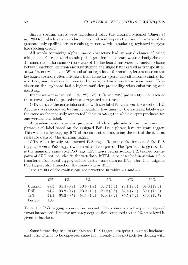
62 CHAPTER 4. EVALUATION TECHNIQUES
Simple spelling errors were introduced using the program Missplel (Bigert etal., 2003a), which can introduce many different types of errors. It was used togenerate only spelling errors resulting in non-words, simulating keyboard mistypelike spelling errors.
All words containing alphanumeric characters had an equal chance of beingmisspelled. For each word to misspell, a position in the word was randomly chosen.To simulate performance errors caused by keyboard mistypes, a random choicebetween insertion, deletion and substitution of a single letter as well as transpositionof two letters was made. When substituting a letter for another, letters close on thekeyboard are more often mistaken than those far apart. The situation is similar forinsertion, since this is often caused by pressing two keys at the same time. Keyscloser on the keyboard had a higher confusion probability when substituting andinserting.
Errors were inserted with 1%, 2%, 5%, 10% and 20% probability. For each ofthese error levels the procedure was repeated ten times.
GTA outputs the parse information with one label for each word, see section 1.2.Accuracy was calculated by simply counting how many of the assigned labels werethe same as the manually annotated labels, treating the whole output produced forone word as one label.
A baseline parser was also produced, which simply selects the most commonphrase level label based on the assigned PoS, i.e. a phrase level unigram tagger.This was done by tagging 10% of the data at a time, using the rest of the data asreference data for the unigram tagger.
GTA relies heavily on assigned PoS tags. To study the impact of the PoStagging, several PoS taggers were used and compared. The “perfect” tagger, whichis the manually annotated PoS tags; TnT, described in section 1.2, trained on theparts of SUC not included in the test data; fnTBL, also described in section 1.2, atransformation based tagger, trained on the same data as TnT; a baseline unigramPoS tagger, also trained on the same data as TnT.
The results of the evaluations are presented in tables 4.1 and 4.2.
0% 1% 2% 5% 10% 20%
Unigram 85.2 84.4 (0.9) 83.5 (1.9) 81.2 (4.6) 77.1 (9.5) 69.0 (19.0)Brill 94.5 93.8 (0.7) 93.0 (1.5) 90.9 (3.8) 87.4 (7.5) 80.1 (15.2)TnT 95.5 95.0 (0.5) 94.3 (1.2) 92.4 (3.2) 89.5 (6.2) 83.3 (12.7)Perfect 100 - - - - -
Table 4.1: PoS tagging accuracy in percent. The columns are the percentages oferrors introduced. Relative accuracy degradation compared to the 0% error level isgiven in brackets.
Some interesting results are that the PoS taggers are quite robust to keyboardmistypes. This is to be expected, since they already have methods for dealing with

4.1. EVALUATING ROBUSTNESS, SEMI-SUPERVISED 63
0% 1% 2% 5% 10% 20%
Unigram 81.0 80.2 (0.9) 79.1 (2.3) 76.5 (5.5) 72.4 (10.6) 64.5 (20.3)Brill 86.2 85.4 (0.9) 84.5 (1.9) 82.0 (4.8) 78.0 (9.5) 70.3 (18.4)TnT 88.7 88.0 (0.7) 87.2 (1.6) 85.2 (3.9) 81.7 (7.8) 75.1 (15.3)Perfect 88.4 - - - - -
Table 4.2: Parsing accuracy in percent. The unigram parser had 59.0% accuracyusing the perfect tagger and 59.2% accuracy using TnT.
unknown words, and most spelling mistakes will result in something that lookslike an unknown word. As long as the suffix is relatively intact, the unknown wordhandling, which usually uses the suffix information, will have relatively little troublein choosing the correct PoS.
While the third digit in the accuracy figures should not be given too muchcredit, since the test data is quite small, it is still interesting to see that bothparsers seem to work better with an HMM tagger than even the perfect tagger.This is likely because the perfect tagger is not really error free. The errors made inthe manual annotation are likely random mistakes, while the errors made by TnTare systematic. It is thus likely easier to generalize from the systematic behaviorthan the more random behavior, despite the difference in accuracy.
The GTA parser seems to be fairly robust, only loosing 15% accuracy when20% of all words are misspelled. This seems to be mostly because of the robustnessof and heavy reliance on the PoS tagging step. The parsing degrades more thanthe PoS tagging, likely because tagging errors will influence the parsing of severalwords in the near context.
There are many programs for finding this type of spelling errors, and suggestingcorrections for them, available. Thus, it might be prudent to ask if a parser reallyhas to deal with these errors, even though they are common in texts. Why not justlet a spelling checker correct all suspected spelling errors using the most probablecorrection suggestion? While it may seem like a good idea, it actually makes theparsing worse than if the spelling errors are left alone.
Spelling errors 1% 2% 5% 10% 20%
With errors 88.1 87.3 85.2 81.7 74.9Automatic correction 87.9 87.1 84.4 80.2 72.4
Table 4.3: Parsing accuracy, in percent, of GTA when errors are inserted. If thetext is automatically corrected by a spelling correction program before parsing, theresults degrade. In both cases the Granska tagger from section 1.2 was used forPoS tagging.

64 CHAPTER 4. EVALUATION TECHNIQUES
Using the spelling checker Stava, described in section 1.2, probably the bestavailable spelling corrector for Swedish (Bigert, 2005b), on our test data resultsin worse results than letting the parser deal with the errors, see table 4.3. Theexplanation is likely that the spelling errors are often not very difficult for theparser, but when an error is corrected using the wrong suggestion the parser hasno clue that something is wrong and sees a possibly quite different sentence. Also,some correct, but unknown to the spelling checker, words are also “corrected”,which of course also makes the parsing harder in the same way.
4.2 Evaluating Robustness, Unsupervised
This section extends the work in the previous section. There, an annotated resourcewas needed. In this section, the overall approach is very similar, but how muchinformation can be gleaned without any annotated resources at all is examined.This research was presented at CICling 2005 (Bigert et al., 2005), where it receivedthe second place best paper award. This work was done together with JohnnyBigert, Ola Knutsson and Magnus Sahlgren.
The Modified Evaluation Method
In the previous section a treebank or similar annotated resource was needed. Nowthe goal is to eliminate the need for such a resource and see how much informationcan be found despite this lack.
Instead of an annotated test set, only an unannotated text collection is required.Apart from this, an estimate of the system accuracy on error free text is also needed.This accuracy is usually known. The first step is to annotate the unannotated dataautomatically with the system that is to be evaluated. This automatic annotationwill be used similarly to how the gold standard annotation was used previously.
Using the system itself as a gold standard on error free text is thus the firstidea. Of course, the system is most likely not 100% correct on error free text, sosome adjustments have to be made to the method to account for this.
If there is an annotated gold standard available, the five cases in table 4.4 canoccur.
The first case, aaa, is usually the most common case, that the system correctlyannotates the word both when errors are present and on error free text. The secondcase, abb, is also quite common, the system fails to annotate some constructioncorrectly and makes the same mistake when there are errors present in the text.The third case, aab, is when an error inserted in the text makes the system fail ona construction it would otherwise have annotated correctly.
Case number four, aba, that the system fails when there are no errors but findthe correct annotation when errors are inserted. It is quite rare, but happens, forinstance when there are two more or less equally probable interpretations for thesystem and the correct one is given a little more weight when the context is changedby some inserted error.
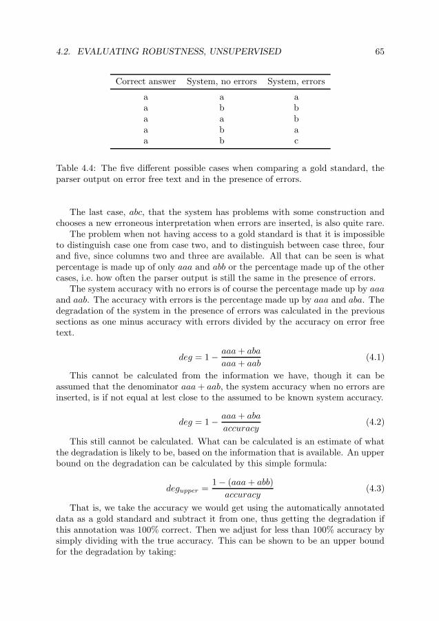
4.2. EVALUATING ROBUSTNESS, UNSUPERVISED 65
Correct answer System, no errors System, errors
a a aa b ba a ba b aa b c
Table 4.4: The five different possible cases when comparing a gold standard, theparser output on error free text and in the presence of errors.
The last case, abc, that the system has problems with some construction andchooses a new erroneous interpretation when errors are inserted, is also quite rare.
The problem when not having access to a gold standard is that it is impossibleto distinguish case one from case two, and to distinguish between case three, fourand five, since columns two and three are available. All that can be seen is whatpercentage is made up of only aaa and abb or the percentage made up of the othercases, i.e. how often the parser output is still the same in the presence of errors.
The system accuracy with no errors is of course the percentage made up by aaaand aab. The accuracy with errors is the percentage made up by aaa and aba. Thedegradation of the system in the presence of errors was calculated in the previoussections as one minus accuracy with errors divided by the accuracy on error freetext.
deg = 1− aaa+ aba
aaa+ aab(4.1)
This cannot be calculated from the information we have, though it can beassumed that the denominator aaa+ aab, the system accuracy when no errors areinserted, is if not equal at lest close to the assumed to be known system accuracy.
deg = 1− aaa+ aba
accuracy(4.2)
This still cannot be calculated. What can be calculated is an estimate of whatthe degradation is likely to be, based on the information that is available. An upperbound on the degradation can be calculated by this simple formula:
degupper =1− (aaa+ abb)
accuracy(4.3)
That is, we take the accuracy we would get using the automatically annotateddata as a gold standard and subtract it from one, thus getting the degradation ifthis annotation was 100% correct. Then we adjust for less than 100% accuracy bysimply dividing with the true accuracy. This can be shown to be an upper boundfor the degradation by taking:

66 CHAPTER 4. EVALUATION TECHNIQUES
degupper = deg + ε (4.4)
ε will now be:
ε =1− aaa− abbaccuracy
− 1 +aaa+ aba
accuracy(4.5)
Using the facts that accuracy is aaa+aab and that aaa+aab+aba+abb+abc= 1:
ε =aba+ aab+ abc
accuracy− aaa+ aab
accuracy+aaa+ aba
accuracy=
2aba+ abc
accuracy(4.6)
Since aba, abc and accuracy are never negative, it follows that ε ≥ 0, i.e. degupperis indeed an upper bound on the degradation.
A simple expression for a lower bound for the degradation is half the upperbound:
deglower =1− (aaa+ abb)
2accuracy(4.7)
In a similar way as before, take:
deglower + δ = deg (4.8)
This gives:
δ =aaa+ aab
accuracy− aaa+ aba
accuracy− 1− (aaa+ abb)
2accuracy=aab− 3aba− abc
2accuracy(4.9)
The suggested lower bound is of course only guaranteed to be a lower bound ifδ is non-negative. Thus, unlike the upper bound which will hold for any system,the lower bound is only guaranteed to hold if:
aab ≥ 3aba+ abc (4.10)
aab is caused by inserted errors causing changes in the annotation of previouslycorrectly annotated text and both aba and abc are similarly caused changes inpreviously incorrectly parsed. Since usually the amount of text that is correctlyannotated is much larger than the amount of errors on text with no errors, this canbe expected to hold quite often.
Both aba and abc occur where the system works poorly, making annotationerrors on error free text. Unfortunately, systems tend to make more changes insuch locations, since there was probably not a clearly favorable interpretation tobegin with. This means that aba and abc will be more common proportionally thanaab, compared to the proportion of originally correctly annotated words, i.e. theaccuracy, aaa+ aab compared to aba+ abb+ abc.

4.2. EVALUATING ROBUSTNESS, UNSUPERVISED 67
Still, for a reasonably accurate system, or an inaccurate system that does notto a very large extent change only annotations of previously failed words, the lowerbound will also hold. For a detailed examination of when the lower bound can beexpected to hold, see (Bigert, 2005a).
When an upper and lower bound is available, the correct value is of coursesomewhere in between. When nothing else is known, guessing that the value isclose to the middle of the bounding interval is an efficient strategy for a goodguess. Thus, an estimate of the actual degradation is:
degguess =3(aaa+ abb)
accuracy(4.11)
Of course, systems that are very robust will tend to have the degradation overestimated. Systems with a very high accuracy will also tend to have the degradationoverestimated, since then the automatic annotation is very close to a true goldstandard, and thus the estimated degradation interval will be quite large comparedto what would be needed. This means that the method could likely be improved,taking these properties into account.
Finally, it is often interesting to know the system accuracy in the presence oferrors, not just the degradation. The system accuracy can of course be calculatedfrom the estimated degradation and the known system accuracy on error free text.
accupper = (1− degrlower) · accuracy (4.12)
acclower = (1− degrupper) · accuracy (4.13)
accguess = (1− degrguess) · accuracy (4.14)
Note that the interval and any error in the guess will be smaller for the accuracythan for the degradation, since the error is multiplied by the system accuracy, whichis less than 1.
Evaluating the Evaluation Method
To see how well the presented method works with real systems and data, severalannotation systems were evaluated using the method. For these systems, manuallycreated gold standards were also available, thus making it possible to see if theestimated degradations and accuracies are close to the true values.
Four different systems were used to evaluate the evaluation method.
• The shallow parser GTA, described in section 1.2, used in the previous section.A gold standard of 14,000 words was used.
• The PoS tagger TnT, see section 1.2, also with a 14,000 words gold standard.

68 CHAPTER 4. EVALUATION TECHNIQUES
• A dependency parser by Nivre (Nivre, 2003), here called MCD, using a manu-ally constructed grammar. It assigns dependency links between words, work-ing from part of speech tagged text. A 4,000 words gold standard was used.
• The Malt parser (Nivre et al., 2004), with a gold standard of 10,000 words.The parser uses the same algorithm as MCD, but uses a memory based clas-sifier trained on a treebank instead of a manually constructed grammar. Italso assigns function labels to the dependency links, unlike the MCD parser.
For all systems, errors were inserted in 1%, 2%, 5%, 10% and 20% of the words,as in the previous section, and for each error level the experiment was repeatedten times. Since the gold standard annotation was available, the true degradationsand accuracies were calculated. The modified evaluation method not using a goldstandard was of course also used, calculating the lower and upper bounds as wellas the guess of the true values. This was also done on a larger test set, consistingof 100,000 words, with no gold standard for any of the systems. The results areshown in tables 4.5 to 4.8 and figures 4.1 to 4.4.
As guaranteed, the true degradation is always below the upper bound. For allsystems the degradation is also above the lower bound, and often quite close to theguessed value. The evaluation on the larger test set also gives very similar resultsas the various smaller data sets.
Error Parse Estimated Real Estimated Reallevel differs degradation degradation accuracy accuracy
1 1.1 0.6 – 1.1 (0.9) 0.9 95 – 95 (95) 952 1.9 1.0 – 2.0 (1.5) 1.6 94 – 95 (94) 945 3.9 2.0 – 4.1 (3.1) 3.6 92 – 94 (93) 9210 7.3 3.8 – 7.6 (5.7) 6.7 88 – 92 (90) 8920 14 7.4 – 15 (11) 13 82 – 89 (85) 83
Table 4.5: Estimated and actual robustness of the TnT part of speech tagger on14,000 words of manually annotated text. Estimated tagger accuracy on error-freetext was 96%.
4.3 Important Points
Evaluation usually entails quite a lot of manual work, either in the form of annot-ating a gold standard resource to evaluate systems on or manually checking systemoutput. As was shown, sometimes it is possible to use one type of gold standardto evaluate other system aspects than the one the gold standard directly supports.More importantly, it was also shown that it can be possible to derive limits on thesystem performance using no manual work at all.

4.3. IMPORTANT POINTS 69
Error Parse Estimated Real Estimated Reallevel differs degradation degradation accuracy accuracy
1 1.2 0.7 – 1.4 (1.0) 0.9 88 – 88 (88) 882 2.3 1.3 – 2.6 (1.9) 1.8 87 – 88 (87) 875 5.1 2.9 – 5.7 (4.3) 4.2 84 – 86 (85) 8510 9.9 5.5 – 11 (8.3) 8.1 79 – 84 (81) 8220 19 10 – 21 (16) 16 70 – 80 (75) 75
Table 4.6: Estimated and actual robustness of the GTA parser on 14,000 wordsof manually annotated text. All figures are given in per cent. Estimated parseraccuracy on error-free text was 89%.
Error Parse Estimated Real Estimated Reallevel differs degradation degradation accuracy accuracy
1 0.7 0.4 – 0.8 (0.6) 0.6 82 – 82 (82) 822 1.7 1.0 – 2.0 (1.5) 1.4 81 – 82 (81) 815 4.0 2.5 – 4.9 (3.7) 3.2 78 – 80 (79) 8010 8.3 5.0 – 10 (7.6) 6.6 74 – 78 (76) 7720 16 9.6 – 19 (14) 13 67 – 74 (71) 72
Table 4.7: Estimated and actual robustness of the MCD parser on 4,000 words ofmanually annotated text. Estimated parser accuracy on error-free text was 82%.
Error Parse Estimated Real Estimated Reallevel differs degradation degradation accuracy accuracy
1 1.8 1.1 – 2.3 (1.7) 1.3 77 – 78 (77) 782 3.4 2.2 – 4.3 (3.2) 2.4 75 – 77 (76) 775 8.7 5.5 – 11 (8.3) 6.1 70 – 74 (72) 7410 16 11 – 21 (16) 12 62 – 70 (66) 6920 30 19 – 38 (29) 23 48 – 64 (56) 60
Table 4.8: Estimated and actual robustness of the Malt parser on 10,000 words ofmanually annotated text. Estimated parser accuracy on error-free text was 79%.

70 CHAPTER 4. EVALUATION TECHNIQUES
1
1
2
2
5
5
10
10
20
20
0.5
error level (%)
degradation (%)
Figure 4.1: Degradation of the PoS tagger TnT. Real degradations are markedwith a *, estimated degradation is the fully drawn intervals, dashed intervals areestimated degradation of TnT using a larger test set with no available gold standard.The dotted lines are the break even points, where the degradation is the same asthe amount of inserted errors.
1
1
2
2
5
5
10
10
20
20error level (%)
degradation (%)
Figure 4.2: Degradation of the GTA parser. The same format as figure 4.1.

4.3. IMPORTANT POINTS 71
1
1
2
2
5
5
10
10
20
20
0.5
error level (%)
degradation (%)
Figure 4.3: Degradation of the MCD parser. The same format as figure 4.1.
1
1
2
2
5
5
10
10
20
20error level (%)
degradation (%)
Figure 4.4: Degradation of the Malt parser. The same format as figure 4.1.


Part II
Useful Applications
73


75
In this part, applications of NLP that can actually be useful for the end userare presented. These include methods for finding errors in text the user produces,creating lexicons for helping the user in understanding foreign languages and auto-matically extracting the important points in long texts.
These applications often rely on the tools presented in the previous section.Examples include grammar checking, which relies heavily on PoS tagging, anddictionary lookup, where compound splitting is used when no translation is availablefor the compound word.


Chapter 5
Grammar Checking
5.1 Introduction to Grammar Checking
Automatic grammar checking is traditionally done using manually written rules,constructed by a computational linguist. Normally, rules are written describingwhat errors look like, what the diagnosis and possible suggestions for correctionsshould be. This can produce very good results, especially regarding high precision.The main drawback is that it takes a lot of time to write and tune the rules. Someerrors types are also hard to capture with rules without producing many falsealarms. It is also hard to write rules for unexpected errors, which can appear forinstance when a writer is not very proficient in the language used, and thus makes“strange” errors compared to native speakers of the language.
Another approach is to write rules for correct language use. Anything thatdoes not match the rules for correct language is then considered wrong. One wayto do this is to write a full parser and flag anything the parser cannot parse asan error. This approach usually has problems with coverage, languages are verycomplex and writing rules describing a language is hard. Usually many correctlanguage constructions are also flagged as errors because of lack of parser coverage,or the parser is written with more general rules that allow many incorrect languageconstructions to slip through too.
Another way of using rules for correct language is to write rules at two differentdetail levels. Rules for errors can then be generated as the difference between thetwo detail levels. A simplified example would be a rule saying that a noun phrasein Swedish contains a determiner and a noun. A more detailed rule would be adeterminer and a noun, agreeing in gender, number and definiteness. Subtractingthe more detailed noun phrase rule from the general one gives for instance rules fornoun phrases with agreement errors in the gender feature. This has been discussedin a finite state automata framework (Karttunen et al., 1966, Sofkova Hashemi etal., 2003).
Methods for detecting grammatical errors without using manually constructed
77

78 CHAPTER 5. GRAMMAR CHECKING
rules have also been used. Some examples: using the probabilities in a statisticalpart of speech tagger (Atwell, 1987), detecting errors as low probability part ofspeech sequences. ProbGranska, described in section 1.2 also works on PoS, com-paring new text to known correct text and deviations from the “language norm”are flagged as suspected errors. Mutual information measurements have been usedto detect incorrect usage of difficult words (Chodorow and Leacock, 2000).
Machine learning has been used to detect when one word has been confusedwith another (Mangu and Brill, 1997). This problem has also been attacked bycombining several methods (Golding, 1995). Comma placement and determiner-noun agreement in Danish has also been treated as a confusion set problem in asimilar way (Hardt, 2001). Another example of a confusion set problem is Englisharticle usage before noun phrases (Han et al., 2004).
In many fields, machine learning is used with an annotated resource as trainingdata. The straightforward way to do this for grammar checking is to annotate acorpus, marking all the grammatical errors. Then a machine learning program couldbe trained on this, resulting in a grammar checking program. This has been triedfor transcribed English spoken language (Izumi et al., 2003). The large drawbackwith this method is that very much manual work is needed for annotating errors intext to avoid data sparseness. This is especially bothersome since there are manydifferent error types, thus very large amounts of data are required. It is also hard tofind all errors in a text manually, since readers often skip over errors when readingtext. On small amounts of data, this method has not produced very impressiveresults.
Statistical and machine learning methods are good for smaller languages, sincethey require few resources to implement. Such methods often only indicate thatsomething is wrong or different from the norm, though. They rarely give a diagnosisor a suggestion for how the problem should be corrected. However, for many writersan indication that something is wrong is enough.
5.2 Evaluating Grammar Checkers
In many areas of natural language processing there are standard ways to evaluateperformance. For instance in tagging and parsing there are standard resources thatpeople can use for evaluation, which has led to steady improvements in these areas.For grammar checking there exist evaluation metrics that are often used, mainlyprecision and recall, but no standard data sets. That there are no evaluationresources for grammar checking is somewhat surprising, since it is a useful andfrequently used application of language processing.
Precision and recall are problematic for grammar checking purposes. Thesemeasures vary wildly between different text types using the same grammar checkingprogram. On text with few errors, for instance newspaper articles, precision isusually low, one typical example from the evaluations in this chapter is 10% for astate of the art grammar checker. If there are only four errors to detect in a text,

5.2. EVALUATING GRAMMAR CHECKERS 79
making a single false alarm means that the maximum achievable precision drops to80%.
On texts with many errors, such as essays written by second language learners,with as much as one error in every three words, the opposite is true: 95% precisionfor the program above. Just selecting word pairs at random and indicating an errorthere can give reasonable precision scores.
Many grammar checking methods make false alarms on (for them) difficultconstructions, whether there are errors present or not. Thus precision is very muchdependent on the number of errors that it is possible to detect, since a large part ofthe number of false alarms is more or less independent of whether there are errorspresent or not.
Precision and recall are also problematic in that not all errors are equally im-portant to find and correct. Keyboard mistypes and erroneous comma placementmight be annoying to the reader, but generally the meaning will be clear. Confusingtwo different words or using the wrong word order might give the text a differentmeaning and could perhaps be much more troublesome for the reader. Unfortu-nately, the errors that are most important to correct are usually the hardest todetect. This means that high precision and recall figures for simple error typesmight be less useful than lower figures for more serious error types. Comparingdifferent systems or evaluating improvements made to a system is thus difficult.
There is also the question of whether the user gets enough information from asuggestion for correction, a correct diagnosis, just a detection or even a detectionwith the wrong diagnosis. Finding a good way to compare different diagnoses etc.is hard.
In this chapter, generally only detection of errors is evaluated, the diagnosis isnot considered. The main reason is that most of the evaluated grammar checkingmethods are statistical methods that do not produce a detailed diagnosis. Theyonly indicate that something is suspiciously different from the reference languagenorm.
Annotation is Hard
When calculating precision and recall, the usual procedure is for a human to lookthrough all alarms and see if they are correct or not. This is the method used inthis thesis. It would be preferable if this could be done automatically, for instanceusing an annotated corpus. This would speed up the process, thus allowing frequentevaluations of small changes to a grammar checking system etc.
Annotating a resource with error information is however hard. It can be hard todetermine what exactly is wrong, even when it is clear that the text is not correct,as for example this text taken from a sign in a train Japan: “Please fall to anImmigration Bureau in 3.4 numbered wire at a station in front of a city hall”. Itcan also be unclear whether a construction is wrong or just unusual. It also happensthat the text is not what the writer intended, i.e. wrong, but still grammatical andeven semantically sound. Should these types of errors also be annotated?

80 CHAPTER 5. GRAMMAR CHECKING
It can also be hard for the annotator to find all the errors, since human readerscome with built in error correction, i.e. often “smooth” over errors, since they“know” what should come next.
How to annotate errors so that it is easy to evaluate grammar checkers lateris also not clear. Which type of diagnosis from the grammar checker should beexpected? When many diagnoses are possible, should the annotation include allof them? It can be hard for the annotator to see all possible analyses of the text.Also, which words should be marked, the ones that are actually wrong or the wholecontext that the error depends on? What is more convenient when evaluating isoften dependent on the grammar checker that is to be evaluated.
One way to get cheap annotation of errors is to use error free text and insertsynthetic errors. Since it is now easy to know where the errors occurred, and whatthe correct text should be, automatic evaluation can often be used. One problem isthat it is not always clear if these measurements tell us anything interesting; doesthe program behave similarly on real errors?
Closing Words
Based on the evaluations in this chapter, current state of the art grammar checkingseems to have very low recall, often less than 30%. Especially for writers that makemany errors. These are the writers that would have had the most to gain froma good grammar checker. This means that more work needs to be done and thatbetter evaluation procedures would be useful, since this has generated progress inother areas.
5.3 Using Chunks for Grammar Checking: ChunkGranska
In section 1.2 the grammar checker ProbGranska is presented. It detects errors intext by searching for unlikely PoS sequences.
In this section the same basic idea is used, but phrase chunks are used insteadof PoS tags. The chunker used has only 8 different chunk types, which means thatthere is no data sparseness problem even for quite long chunk sequences. It alsofinds different error types than ProbGranska, since different error types show upon the chunk level and on the PoS level.
This research was first presented at Nodalida 2005 (Sjöbergh, 2005a). Thepresented method creates a grammar checking tool without using any manual workonce a chunker is available. Only the chunker and unannotated text with relativelyfew errors is required.
In this section, chunking means dividing sentences into non-overlapping phrases.The sentence “The red car is parked on the sidewalk.” could be chunked as “[NPThe red car] [VC is parked] [PP on the sidewalk]” where NP means noun phrase,VC means verb chain and PP means preposition phrase. Chunking is a relativelywell developed field of research. There are chunkers available for several languagesthat give good results, usually well over 90% accuracy.

5.3. USING CHUNKS FOR GRAMMAR CHECKING: CHUNKGRANSKA 81
The GTA shallow parser, see section 1.2, is used for chunking, discardingeverything except the top level phrase information and inserting a special boundarychunk tag at clause boundaries indicated by GTA.
The Grammar Checking Method
To create a grammar checker a chunker and an unannotated corpus is needed. First,the corpus is automatically annotated using the chunker. Statistics such as chunkn-gram frequencies are collected, giving reference statistics for normal language use.
When a new text needs to be checked, the chunker is run on the new text. Ifthis new text contains chunk sequences that never occurred in the reference texts,they are marked as possible errors. Of course, a higher threshold for believinga construction is correct could also be used, for instance if the reference text issuspected to contain many erroneous constructions.
The number of different chunk types, while varying depending on the languageand chunker in question, is generally quite low. The only requirement on thecorpus is that it should contain relatively high quality texts, so creating a verylarge reference corpus is often possible. This means that very good statistics canbe collected even for quite long chunk sequences. Hence, there are few false alarms,since even rare chunk sequences will normally be present in the reference corpus.Using only chunk sequences, even for n-grams of length five, less than 10 false alarmswere generated on 10,000 words of text in the evaluations, with slight variationbetween different genres.
While it is possible to use the method with long chunk sequences it is probablybetter to use shorter n-grams. Since there is no detailed error diagnosis available,it is not that helpful to get an error report indicating that something is wrong witha very long text sequence. Pointing out shorter sequences makes locating the erroreasier.
While the reliable statistics lead to very few false alarms, it turns out that notthat many true errors are detected either. One example from the evaluations was13 correct detections and one false alarm on data where other grammar checkersdetected between 60 and 100 errors, though with more false alarms.
To detect more errors the chunk set can be modified. The modifications can bedone completely automatically without changing the chunker. If we are interestedin finding errors related to verb usage, we can substitute the chunk used for verbchains with the actual words of the chunk. So for the example sentence “[NP Thered car] [VC is parked] [PP on the sidewalk]”, originally the chunk trigram “NP-VC-PP” is produced. With the new modification “NP-is parked-PP” is producedinstead. This allows detection of new error types, for instance wrong verb tense, asin “I want to went home” or “I thought he is nice”. Similarly, if we want to finderrors related to prepositional use we can do the same for preposition phrases. Thisdetects errors such as “I arrived on Stockholm”.

82 CHAPTER 5. GRAMMAR CHECKING
While this has the benefit of detecting many new errors it also has drawbacks.The number of chunk types is no longer small, it is very large. Thus the statisticsbecome sparse, leading to many false alarms.
A better approach in a similar vein is to change only those verb chains orpreposition phrases which are common, i.e. occur more than some threshold numberof times in the reference corpus. If the limit is high enough it works quite well.The statistical data is still reliable. This gives more correct detections while onlygiving a few more false alarms. Of course, not all the errors detected by the moreaggressive strategy of replacing all verb chain chunks are detected with this lessaggressive method. It is easy to tune the aggressiveness by simply changing thethreshold value. This means that users that accept more false alarms if more correctdetections are produced can choose a different setting than users that want fewerfalse alarms at the cost of more remaining errors.
The GTA chunker can produce more detailed information for noun phrases,such as head noun, if the phrase as a whole acts as plural or singular, definite formor indefinite etc. This information can be used in the same way as exchangingpreposition phrases for their content words. Adding the information to the chunktag allows detection of more errors, such as “these are my the cars”, but of coursealso makes the statistics more sparse, leading to more false alarms.
adverb phraseadjective phraseboundary (clause or sentence)infinitive phrasenoun phrasepreposition phraseverb chainoutside of phrase (e.g. punctuation or interjections)
Table 5.1: The chunk types used.
Evaluation
The method was evaluated on Swedish texts. As reference texts the Swedish Parolecorpus of about 16 million chunks, and the KTH News Corpus of about 10 millionchunks, both described in section 1.2, were used. The evaluation was performedon three different genres: newspaper texts, student essays and essays by secondlanguage learners of Swedish. All error reports were manually checked to see ifeach error was a genuine error or a false alarm. The texts were not checked forundetected errors.
In the tests, chunk n-grams are allowed to span sentence boundaries, thoughthere is a boundary tag inserted in the chunk sequence at all sentence boundaries.

5.3. USING CHUNKS FOR GRAMMAR CHECKING: CHUNKGRANSKA 83
N-gram length Limit Correct False
3 500 4 633 5,000 2 73 50,000 1 24 500 14 1794 5,000 6 524 50,000 3 195 500 26 2795 5,000 17 1445 50,000 15 74
Table 5.2: Evaluation results on 10,000 words of newspaper texts, taken from theSUC corpus. There are very few errors in these texts, which leads to poor accuracy.
N-gram length Limit Correct False
3 500 75 203 5,000 24 23 50,000 5 14 500 223 434 5,000 98 124 50,000 33 65 500 315 605 5,000 199 275 50,000 108 13
Table 5.3: Evaluation results on 10,000 words of second language learner essaysfrom the SSM corpus. With many errors to detect, it is easy to get quite highprecision. Most errors in the text go undetected, though.
Common verb chains and preposition phrases were replaced with the word se-quence they represented, for different threshold values for what was considered com-mon. Noun phrases were replaced with a tag indicating the type of noun phrasefound, such as a genitive form or a definite and plural form. A list of the chunktypes used is shown in table 5.1.
In tables 5.2, 5.3 and 5.4 the results using different n-gram lengths and differentlimits for when to consider a chunk “common” are presented for three differentgenres.
Other grammar checkers have also been evaluated on these texts, and someresults from those are also presented, in tables 5.5, 5.6 and 5.7, to give an ideaof how good the chunk method is in comparison. The two best grammar checkers

84 CHAPTER 5. GRAMMAR CHECKING
N-gram length Limit Correct False
3 500 26 473 5,000 12 113 50,000 6 14 500 93 1384 5,000 42 474 50,000 24 135 500 174 2335 5,000 118 1385 50,000 68 69
Table 5.4: Evaluation results on 10,000 words of native speaker student essays fromthe written part of the Talbanken corpus. Frequent use of quotations leads to manyfalse alarms.
MS Word Granska
All detected errors 10 8All false positives 92 35
Detected spelling errors 8 6False positives 89 20
Detected grammar errors 2 2False positives 3 15
Table 5.5: Evaluation of two state of the art grammar checking methods onproofread newspaper texts, 10,000 words. Table 5.2 shows the chunk method onsimilar data.
MS Word Granska
All detected errors 392 411All false positives 21 13
Detected spelling errors 334 293False positives 18 5
Detected grammar errors 58 118False positives 3 8
Table 5.6: Evaluation of two state of the art grammar checking methods on secondlanguage learner essays, 10,000 words. Table 5.3 shows the chunk method on thesame data.

5.3. USING CHUNKS FOR GRAMMAR CHECKING: CHUNKGRANSKA 85
MS Word Granska
All detected errors 38 48All false positives 31 13
Detected spelling errors 24 17False positives 28 0
Detected grammar errors 14 31False positives 3 13
Table 5.7: Evaluation of two state of the art grammar checking methods on essayswritten by native speakers, 10,000 words. Table 5.4 shows the chunk method onthe same data.
evaluated on these texts were MS Word 2000 and Granska, see section 1.2. Bothare based mainly on manually constructed rules for different error types.
The test genres were newspaper texts, essays by native speaker students andessays by second language learners. The newspaper texts were taken from the SUCcorpus, see section 1.2, which contains almost no errors. The writers also have a verygood grasp of the language and use many “advanced” language constructions. Thestudent essays were taken from the written part of the Talbanken corpus (Einarsson,1976). The essays are argumentative, discussing the views expressed in some othertexts the writers have read, and they quote a lot from these texts. The secondlanguage learner essays were taken from the SSM corpus, described in section 1.2.The language proficiency varies from writer to writer, some have studied Swedishfor only a few months while some have studied several years. These essays areusually quite short.
Looking in the tables, it can be seen that the method is easy to tune to producefew or many error reports. The optimal choice is probably different for differentusers. Writers with a good grasp of the language using many varied constructionswould likely use a very high limit for “common” phrases, while users with limitedknowledge of the language and thus less productive use of their vocabulary wouldbenefit more from a lower limit. An experienced writer might also benefit morefrom reports of errors on long chunk sequences, probably being able to assess whatis wrong and also capturing error types with longer dependencies. An inexperiencedlanguage user would probably be better served with a more precise diagnosis, i.e.use shorter n-grams, to understand what is wrong.
On newspaper texts there were almost no errors to detect. A reasonable per-formance level to choose on this genre is perhaps 3-grams and the highest limit for“common” chunks. This gives one correct detection and two false alarms. No othergrammar checkers were evaluated on this text, but on similar newspaper texts, also10,000 words (which were not used in these evaluations, since they turned out tobe part of the reference corpus in these experiments), gave two detected errors and

86 CHAPTER 5. GRAMMAR CHECKING
three false alarms for MS Word 2000, which was the best performing grammarchecker on this genre. This is while not counting simple spelling errors, otherwisethe best grammar checker was Granska which had 8 correct detections and 35 falsealarms. No grammar checker had less than 35 false alarms when counting spellingerrors.
The best performing grammar checker on essays written by non-native speak-ers was Granska, which detected 411 errors and made 13 false alarms, which is alot more than the chunk based method detects, see table 5.3. However, most ofthe 411 detected errors are simple spelling errors, which will generally be ignored,since the chunker ignores them. If only grammatical errors and hard spelling errors(errors resulting in another existing word) are counted, the best performing gram-mar checker detects 118 errors, making 8 false alarms. Using 4-grams of chunksand a limit of 5,000 occurrences for “common” chunks, the chunk method performssimilarly, with 98 correct detections and 12 false alarms. MS Word 2000, which istuned for high precision, detected 58 errors with only 3 false alarms on this text,not counting spelling errors.
There are very many errors in these essays, most of which were not detected byany of the grammar checkers. Since there are so many errors and since even trigramsof chunks can span quite a lot of text, finding n-grams of chunks with errors in themmight be thought to be too easy. While it is true that there are many errors in thetexts, just pointing out random chunk n-grams does not perform that well. Whenchecking 50 random chunk trigrams, 27 would be counted as correctly detectederrors and 23 as false alarms. The chunk based method presented here performsbetter than this.
On the student essays MS Word 2000 detected 14 errors with 3 false alarmsand Granska detected 31 with 13 false alarms. When including spelling errors MSWord detects 38 errors with 31 false alarms and Granska 48 errors, still with 13 falsealarms. A reasonable performance level for the chunk method here is 24 correctdetections with 13 false alarms, which is not so good.
The chunk method performs quite poorly on these essays. This is mainly causedby them differing a lot from the reference domain, while still using correct languageconstructions. The main problem is that there are a lot of “short quotes” whichare rare in the reference texts and thus give rise to many unseen chunk n-grams.There are also longer quotes from “odd” genres, such as old bible translations andlaw books, which while not erroneous are not examples of the more common use ofSwedish, and thus lead to more false alarms.
Discussion
Many of the unseen n-grams are caused by chunker errors, i.e. the unseen chunkn-gram is not the n-gram that should be produced by a 100% correct chunker.Usually the reason the chunker makes an error is because there is an error in thetext, which means that this is not a problem. The method correctly signals anerror.

5.4. USING THE INTERNET FOR GRAMMAR CHECKING:SÖKMOTORGRANSKA 87
As mentioned regarding the poor performance on the native speaker studentessays, the method has problems with texts from domains that differ a lot from thedomains the reference texts come from. In general this is not a great concern, sinceit is cheap to add more data to the reference texts. All that is needed is raw text,although with relatively few errors.
Increasing not only the number of domains covered by the reference texts, butalso just increasing the size of the reference data is generally a good idea. Sinceit is so cheap it is a good way to reduce the number of false alarms. False alarmsare generally caused by rare language constructions being used, which is mitigatedby a larger reference corpus. A larger reference corpus also gives a richer chunk setfor a fixed limit on occurrences for “common” chunks, which can also lead to morecorrect error detections.
This method detects many different types of errors. Some error types detectedby it are considered “hard” to detect by manually writing rules to detect them, andare thus not very well covered by traditional grammar checkers. This is one reasonthe chunk method detected errors that no other evaluated grammar checker found.
The main error types detected by the method in these experiments were missingor erroneously placed commas, word order errors, spelling errors resulting in otherexisting words and using the wrong preposition for a certain verb. Other errortypes with fewer detections were verb tense errors, split compounds, missing words,missing sentence breaks, agreement errors, other inflectional errors, repeated words,unconventional use of fixed expressions and idioms and simply using a differentword from the one intended (this error type was only made by the second languagelearners).
Since the method detects many different types of errors but does not give adetailed diagnosis it is perhaps hard for a user to understand what is wrong. Oneway to mitigate this is to create different versions of the grammar checker. Oneversion could for instance use the changing of chunk tags for verb chains and thusdetect mostly verb related errors, while another might change the chunk tags fornoun phrases and thus find noun related errors. They will likely all detect someerror types related to chunk sequences in general, but those that only one versiondetects could be given a slightly more detailed diagnosis.
5.4 Using the Internet for Grammar Checking:SökmotorGranska
A lot of research has recently focused on the fact that very simple methods canoften give interesting results, as long as they have access to very large amountsof data. This can go as far as outperforming sophisticated methods using smalleramounts of data.
The Internet is a large and freely available corpus, so it is appealing to use it fordifferent purposes. Some work using approaches similar to the one in this sectioninclude estimating bigram frequencies for rare bigrams (Keller and Lapata, 2003),

88 CHAPTER 5. GRAMMAR CHECKING
suggesting improvements on text constructions where the author is unsure (Moréet al., 2004) and detecting malapropisms (Bolshakov, 2005).
Since the statistics on chunks used in the previous section is very good evenin small corpora, one idea is to go in the other direction. Why not use very largecorpora, such as the Internet, and just use word sequences? Then we would noteven need a chunker or tagger.
In this section, this method of grammar checking is explored. Two main ap-proaches are used: marking language constructions not present on the Internet assuspected errors and using the Internet to filter out false alarms from other grammarchecking methods. This section is based on the paper “The Internet as a NormativeCorpus: Grammar Checking with a Search Engine” (Sjöbergh, forthcominga).
When using the Internet as an example of correct language use, as we do here,there are some problems. There are many web sites with intentional examplesof incorrect language use, and recognizing these can be hard. Publishing text onthe Internet is cheap and easy, with no requirements regarding proofreading, sothere are also many unintentional errors. These problems are not that bad inpractice, since there are usually more examples of correct constructions than thecorresponding erroneous constructions. As long as the possibility of errors is takeninto account, many methods using the Internet as a normative corpus work quitewell.
Another problem is that while the Internet is large, it is too small for manyinteresting ideas. This is harder to deal with, but the Internet is still growing quitefast, so just by waiting more and more data is made available.
Internet Size
Word Internet Parolepages occurrences
välde 4,190 33multnade 121 1ett 3,710,000 139,766den 5,080,000 199,223
Table 5.8: Occurrences in a 20 million words corpus and using an Internet searchengine.
When using the Internet as a large corpus it is interesting to know roughly howlarge it is. Since it grows all the time there is no official size available. The sizealso varies depending on the search engine (or other method) used to access it.
The search engine eniro.se was used in these experiments. While other searchengines give access to more documents, this one has some advantages. The outputis very easy to parse, there is no limit on the number of searches each day and it
5.4. USING THE INTERNET FOR GRAMMAR CHECKING:SÖKMOTORGRANSKA 89
has an “only pages in Swedish” option, which was useful since the evaluations ofthe methods were done on Swedish texts.
Using the Internet search engine eniro.se with the “only pages in Swedish”option enabled, searches were done for a few words chosen more or less at random.Some relatively rare words, which probably occur only a few times on each webpage, and some common words, which probably occur many times on each page.The number of pages returned by the search engine was then compared to thenumber of occurrences of the words in the Swedish Parole corpus, described insection 1.2.
For the rare words there were about 100 times more pages than occurrencesin the corpus. For common words there were about 25 times more pages thanoccurrences in the corpus, see table 5.8 for some examples. This difference betweencommon and rare words is of course caused by the common words occurring manytimes on each page in the search engine.
The Parole corpus contains 20 million words, so a low estimate would give a fewbillion words of Swedish indexed by this search engine. Swedish is a relatively largelanguage on the Internet, though not very large in the number of speakers. Englishis of course the number one language on the Internet, with a very large margin tolanguage number two.
These numbers give a rough idea of what sort of statistics are reasonable tocollect. For instance word trigram occurrences would not be reasonable, since evena low estimate of 100,000 possible word forms would lead to very sparse data indeed.In the next section we would like to use occurrences of n-grams of words, but evenfor bigrams the data will be sparse.
Detecting Errors
An idea similar to ProbGranska, see section 1.2, or the chunk based grammarchecker in section 5.3 was used to detect errors. All word bigrams in a text weresent to a search engine. Bigrams not occurring on the Internet were reported aserrors. This was tried on newspaper texts and on essays written by learners ofSwedish.
Errors found included spelling errors, erroneously split compounds, agreementerrors, missing words and more. Example errors include: “sådana prisen” (“suchthe price”, agreement error), “hav miljon” (“sea milion”, spelling error resulting inanother word, “halv miljon” “half a milion” was intended) and “arbetar restaurang”(“works restaurant”, a missing preposition). Results can be seen in table 5.9.
The results were compared to two state of the art grammar checkers, MS Word2000 and Granska, see section 1.2. They not unexpectedly outperform the Internetmethod, mostly because they detect a lot of spelling errors but also because theydetect errors using a larger scope than this method.
Since the Internet is too small for good coverage of Swedish word bigrams thereare many false alarms from the Internet method, especially on the newspaper texts.

90 CHAPTER 5. GRAMMAR CHECKING
Checking only bigrams where both words are common mitigates this, but lowersrecall. All spelling errors go undetected, for instance.
Method Genre Limit Correct False
Internet newspaper 10,000 1 21Internet newspaper 100 2 162Granska newspaper - 8 35MS Word newspaper - 10 92
Internet learner 10,000 21 4Internet learner 100 100 22Internet learner 0 283 27Granska learner - 411 13MS Word learner - 392 21
Table 5.9: Using word bigrams to detect errors, in newspaper texts and secondlanguage learner essays. “Limit” is the minimum number of occurrences on theInternet of each word required to try the bigram lookup.
The performance on newspaper texts is quite bad, but on the other hand thereare almost no errors in the text so very few detections can be expected. On thesecond language learner essays quite good results are achieved, comparable to stateof the art grammar checkers. Learners use a limited vocabulary, mainly commonwords, which is well covered on the Internet. Hence, there are few false alarms.Learners also make many errors detectable by this method.
This method only finds very local errors. It also has problems with phrase andclause boundaries and some multi-word expressions, and of course rare words. Someimprovements include ignoring numbers, interjections and proper names, which canbe identified relatively well with automatic methods.
Data is still very sparse for normal language users, since there are several hun-dred thousand word forms that are commonly used, and only a few billion wordsof text are available in the “corpus”. This means that a bigram in general has verylow probability of occurring on the Internet.
Other than being very resource lean, the Internet method also has anotheradvantage. Of the 21 detected errors in learner essays checking only common words,8 errors were not detected by any of four other available grammar checkers, the twostate of the art methods above and ProbGranska, see section 1.2, and SnålGranskafrom section 5.5. When checking only such bigrams the number of false alarms isvery low.
This indicates that this method can be used together with other methods. Thiswould improve error coverage while introducing very few new false alarms.

5.4. USING THE INTERNET FOR GRAMMAR CHECKING:SÖKMOTORGRANSKA 91
Removing False Positives
Another use of the Internet is to remove false positives (false alarms). Instead ofletting the lack of certain constructions be an indication that they are wrong, theoccurrences of certain constructions can be used to indicate that they are correct.
This can be done by taking the suspected errors from a grammar checker andsending these constructions to a search engine. If these have been used a sufficientnumber of times on the Internet, treat the suspected error as a false alarm. It isa good idea to require more than one occurrence on the Internet, since there arebound to be some errors, intentional or otherwise, on the Internet.
This was tried for two different grammar checkers. Both are based on automaticmethods and thus have a tendency to produce quite many false alarms, especiallyon text domains that differ from the training texts.
ProbGranska
ProbGranska, described in section 1.2, detects unlikely PoS trigrams. This leads toquite a lot of false alarms in general, because the PoS trigram data is quite sparse.ProbGranska already has strategies to mitigate this, but the Internet can be usedto remove more false alarms.
Detections False Alarms Precision
Original 102 19 84%Filtered 84 7 92%
Table 5.10: Filtering suspected errors from the grammar checker ProbGranska usingthe Internet. Evaluated on essays written by second language learners.
ProbGranska points out PoS trigrams as suspected errors. For each such trigramthe corresponding trigram of words sent to a search engine. If there were more than25 hits with the search engine the error was removed as a false alarm.
This gives the filter a shorter scope than the original error detection. The filteronly looks at three words, while the tagging step that produces the PoS trigramcan look at the neighboring words and their PoS as well.
When tried on 10,000 words of learner essays precision was increased from 84%to 92%, but quite a few of the correct detections were also removed, see table 5.10.On 10,000 words of newspaper texts, 16 of 36 false alarms were removed. Sincethere were very few errors in these texts, there was only one correct detection. Thecorrect detection was not removed.
Split Compounds
Split compounds is a quite common error type in Swedish (and other compoundinglanguages, such as German). It is quite hard to detect these errors with automatic

92 CHAPTER 5. GRAMMAR CHECKING
Split Other Falsecompounds errors alarms
Original 19 27 10Filtered 16 (0) 3 (19) 0 (3)
Table 5.11: Filtering suspected split compounds from the grammar checker Snål-Granska, in second language learner essays. Numbers in parenthesis are detectionswhich remain but had the diagnosis changed to “other error type”.
methods, and few grammar checkers for Swedish try to handle this error type. Thereare many (erroneous) split compounds on the web, which means that checking ifthe suspected error occurs on the Internet is not a very good way to filter falsealarms for this error type. Too many correct detections are removed.
For split compounds of Swedish, one can instead combine the words of thesuspected split compound into a compound word. If this word exists on the Internetit was a correct alarm, otherwise it was a false alarm.
This removes many false alarms. This also removes detections of errors whichare not split compounds but still erroneous. Some error types sometimes look likesplit compounds, examples include agreement errors and using the wrong wordclass, such as adjective form instead of adverb, noun instead of verb. It wouldprobably be good for the writer to get an error report on such errors, even if thediagnosis was “split compound”.
Still, it would be better if they were detected with the correct diagnosis, perhapsby a different grammar checker module. If a good split compound detection moduleis to be created, these should be removed.
It is possible to modify the simple filtering method above to handle such errorsbetter. The words are combined into a compound as before. If this compound ismore common than the original multi-word expression it is treated as a correctlydetected split compound. If neither the compound nor the multi-word expressionoccurs on the Internet more than 10 times it is probably not a split compound, butit is probably still an error. These detections are given another diagnosis, such as“error, but not a split compound”.
The grammar checker SnålGranska, see section 5.5, detects split compound er-rors (and some other error types). It has quite good recall for these errors comparedto other grammar checkers. It has a relatively low precision though, so there is po-tential for improvement by removing false alarms.
When using the first mentioned method to remove false alarms for split com-pounds 16 of 29 split compound false alarms are removed on 10,000 words of news-paper text. Using the filter that relabels errors only removes 5 false alarms, whilethe other 11 are relabeled. There were no correct detections of split compounds inthese texts, since there were no errors to detect.
On second language learner essays there are more errors to detect. The filter

5.5. USING MACHINE LEARNING FOR GRAMMAR CHECKING:SNÅLGRANSKA 93
removes most false alarms and also correctly relabels most errors of other types,see table 5.11. 16 of 19 correctly detected split compounds remain, with the correctdiagnosis. 3 errors of other error types are still labeled as split compounds and 3false alarms remain, though no longer believed to be split compounds.
Discussion
While the Internet is often too small for normal users it might be large enough forspecial applications. One example is learners of a new language, who use a limitedvocabulary. This vocabulary tends to be common words, and thus well covered onthe Internet.
The Internet can also be used as a complement to traditional methods, byfor instance removing false alarms or detecting some error types missed by othermethods.
5.5 Using Machine Learning for Grammar Checking:SnålGranska
In this section a method for constructing a grammar checker using machine learningis presented. To avoid the time consuming annotation of training data, artificialerrors are used instead of real errors. The main strength of the method is thatit is very resource lean, requiring little in the way of manual work and availableresources. This research was done together with Ola Knutsson, and it was presentedat RANLP 2005 (Sjöbergh and Knutsson, 2005).
General Method
The basic idea of the method is to treat grammar checking as a tagging task. Collecta lot of text, mark all errors with “ERROR” and all other words with “OK”. Trainan off-the-shelf tagger on this data and you have a grammar checker. To achievebetter feedback it is possible to have different tags for different types of errors, i.e.“SPELLING”, “VERB-TENSE”, etc. Another way to achieve this is to train a newspecialized classifier for each error type, which ignores other types of errors.
Finding these errors and annotating them requires a lot of work. This is hereavoided by using artificial errors. A lot of text without errors is used, and the textis then corrupted by adding errors. Since they are added automatically they canbe annotated at the same time.
When this is done, the resulting text is automatically annotated with PoS, hereusing TnT, see section 1.2. The words, PoS and error annotation are then used astraining data for the automatic grammar checker. Almost any machine learningimplementation could be used for this. Here, fnTBL described in section 1.2 wasused. One reason was that it produces rules that are easy to understand for nontechnical humans. This means that it is easy to check the results to see if they are

94 CHAPTER 5. GRAMMAR CHECKING
interesting, and that it is possible for for instance a linguist to go through the rulesand possibly change them after the learning is done.
When generating the artificial errors it is likely that the more “human like” theerrors are, the better the grammar checker will be. Of course, using real humanproduced errors would be best, since that would give the machine learner a properview of what errors look like. Since the strength of the method is that it is resourcelean, though, focus was not put on producing realistic errors. If a lot of effort isspent on producing artificial errors it would perhaps have been more useful to createa traditional grammar checker. As long as the resulting grammar checker is useful,the simpler the error generation the better, so very simple artificial errors wereused. About 30 minutes of manual work was used in creating the error generationprograms for both the error types tested. This is all the manual work that is neededto create the grammar checker.
In figure 5.1 an example of an error generation program, for agreement errors,is shown. When implemented in a high level scripting language, the code is notmuch longer than this pseudo code.
(1) Read lemma lexicon (or stems)(2) Read PoS tags with agreement constraints(3) Run PoS tagger(4) For each tagged sentence:(5) Pick random word with agreement constraint(6) Get lemma (lexicon)(7) Get random word with this lemma (lexicon)(8) If not exact same word:(9) Change word, mark as error
Figure 5.1: Example of error generation code, for generating agreement errors.
If the error generation code is run on “I bought a car.” we could get for instance“I/OK bought/OK a/OK cars/ERR ./OK”.
The error generation programs sometimes change a sentence so that the resultis still grammatical. One simple example would be a program that inserts wordorder errors by randomly changing the order of neighboring words. Not all changeswill lead to errors, for example “I heard dogs barking” and “I heard barking dogs”are both correct, but “heard I dogs barking” is not. Such sentences will of coursestill be marked as erroneous. This is not a great problem, since if something iscorrect there are usually many examples of this which are not the result of changes,and thus marked as correct. This means that the learner will in general only learnrules for those artificial errors that result in text which is incorrect, since the other“errors” will be drowned out by all the correct examples.
This method can be used on many error types. Some examples of errors thatcould be generated artificially include: word order errors (reorder randomly se-lected words), missing words (remove randomly selected words), “hard” spelling

5.5. USING MACHINE LEARNING FOR GRAMMAR CHECKING:SNÅLGRANSKA 95
errors (replace words with another word with only a one letter difference), splitcompounds (replace all words that could be made from concatenating two otherwords in the corpus with these two words), agreement errors and verb tense errors(use a dictionary lookup to replace words with another inflectional form of the sameword), prepositional use (change prepositions to other prepositions), etc.
The main strength is errors that are simple to generate, but where the resultingsentence structure is hard to predict. Word order errors and split compounds areexamples of such errors. Errors such as repeated words for which it is straight-forward to predict the result can also be handled by this method, but is probablybetter handled by traditional methods.
The method was tested on two different error types: split compounds, an errortype suited to our method, and agreement errors, suited to traditional grammarchecking methods. Agreement errors were tested to see how the method holds upwhere the competition is the hardest. The method was evaluated on Swedish textand compared to three other grammar checkers.
Error Type 1: Split Compounds
In compounding languages, such as Swedish and German, a common error is tosplit compound words, i.e. write “quick sand” when “quicksand” was intended.Two concrete examples from Swedish: (1) “en långhårig sjukgymnast” means “aphysical therapist with long hair”. Splitting the compounds to make “en lång hårigsjuk gymnast” is still grammatical but the meaning is changed to “a tall, hairyand sick gymnast”. (2) If the compound “ett personnummer” (“social securitynumber”) is split to “ett person nummer” (“one person number”) it would lead toan agreement error and be ungrammatical.
The SUC corpus, see section 1.2, was used as training data for the machinelearner. The Stava spelling checker, also described in section 1.2, was used toautomatically split compounds. The research on compound splitting presented insection 3 was carried out after these experiments, otherwise those methods couldof course also be used. Even simpler methods, such as splitting words if they canbe constructed from two other words in the corpus, could also be used.
While some manual work has been put into creating Stava (and thus in a sensemade this type of error generation less independent of manual work), the part usedhere, i.e. the compound analysis component, was automatically constructed from adictionary. If however there are tools available that someone already put a lot ofmanual effort into creating, the method described here could of course use these.It would then be a method of creating a grammar checking component from othertools in an unsupervised way.
The training data consisted of the corpus texts, to show correct language use,and another copy of all the corpus texts. The second copy had all compounds recog-nized by the compound splitter split into their components, with the componentsmarked “error”.

96 CHAPTER 5. GRAMMAR CHECKING
The rule learner was given the word n-grams, PoS n-grams and error annotationn-grams. The n-grams were unigrams, bigrams and trigrams. Some combinationsof these were also allowed, such as the current word and error annotation trigrams.The initial guess for the learner was that words more common in compounds thanas a single word (in the training data) were probably errors and all other wordscorrect. The best rules found by the learner used PoS bigrams or error annotationof one word and PoS of its neighbor.
To improve the precision of the learned rules the fact that if a compound issplit it will result in at least two components can be used. Any single word markederror is thus probably a false positive (or one of its neighbors is a false negative),and can be removed. Since there was a spelling checker available we improved thisa little by filtering the output through the spelling checker. If a suspicious wordcould not be combined into a correct compound by using a neighboring word alsomarked “error” it was considered a false alarm and the error was removed. Thisimproved the precision but also removed many correctly detected split compounds,usually because they were misspelled as well as erroneously split (and would thusbe found by the spelling checker instead).
Using the spelling checker gave only a very small improvement over just remov-ing errors with no neighboring error, while both methods improved the precision ofthe original rules significantly.
Error Type 2: Agreement Errors
In Swedish, determiners, adjectives, possessives and nouns must agree in number,gender and definiteness. Agreement errors are quite common, especially when re-vising text using a computer. The agreement can span long reaches of text, whichcan make the errors hard to detect. Manually writing good rules for agreementerrors is relatively straightforward, and it is one of the more popular error categor-ies to detect among automatic grammar checkers. Though manually created rulesusually detect agreement errors with high precision, the recall is often low.
To generate artificial errors the SUC corpus was used again. In each sentence aword from any word class with agreement restrictions was randomly selected. Thisword was then changed to another randomly selected form of the same word. Thiswas done by a simple lexicon lookup were the lemma of the word was found andanother word with the same lemma and a different surface form was selected. Theselected word was marked as an error and all other words were marked as correct.
When an agreement error occurs, at least two words are involved. This methodonly marked the changed word as an error, although it would also be reasonableto mark all words with agreement restrictions related to the changed word. Onereason for doing it this way is that it is easy to mark the changed word but hardto mark the other words. If they could be found, the same method could be usedto detect agreement errors. Also, since here it is known which word was changed,which word should be corrected to retrieve the intended meaning is thus known,even though the agreement error itself could likely be corrected in several ways.

5.5. USING MACHINE LEARNING FOR GRAMMAR CHECKING:SNÅLGRANSKA 97
MS Word Pr.Gr. Granska SnålGr. SnålGr. Base Base Union Inter-
+ filter + filter section
Detected 75 225 322 588 535 331 120 582 275False neg. - - 490 224 277 481 692 230 537False pos. - - 6 49 24 162 6 29 1
Prec. (%) - - 98 92 96 67 95 95 100Rec. (%) - - 40 72 66 41 15 72 34
Table 5.12: Detection of split compound components. The baseline “Base” is simplythe most common tag for each word (“error” or “correct”), from the training data.“Union” is any word marked “error” by either the manual rules of the Granskagrammar checker or the filtered automatic rules of SnålGranska (the presentedmethod). “Intersection” is any word marked by both. MS Word and ProbGranskado not specifically address the problem of split compounds but find some anyway,but of course with a different diagnosis.
As features for the machine learner the gender, number and definiteness of theword were given (if applicable). All this information is included in the tag set TnTwas trained on, and was automatically assigned. The PoS of the word and the errorannotation were also included. Unigrams, bigrams, trigrams and combinations ofthese features were used. The best rules combined PoS and n-grams of the genderfeatures.
The initial guess was that there were no errors in the text. A baseline wasconstructed by locating every occurrence of two consecutive words that had differentgender, number or definiteness and marking the first of these as an error. Thisbaseline could be used as initial guess for the learner, which gives higher precisionthan the original initial guess, since many rules are learned that remove alarms(mostly spurious alarms from the baseline), but lower recall.
Evaluation
The method was evaluated and compared to Granska and MS Word 2000, and alsoto the ProbGranska statistical grammar checker. All three are described in section1.2.
Evaluation on Collections of Errors
The first evaluation was performed on collections of examples of authentic splitcompounds and agreement errors. These were all taken from real texts, but sincethere is at least one error in each sentence it is a quite unrealistic data set, andit is easy for the grammar checkers to achieve high precision with so many errorsavailable. The benefit of these collections is that all errors that occur have been

98 CHAPTER 5. GRAMMAR CHECKING
MS Word ProbGr. Granska SnålGr. Baseline Union Intersection
Detected errors 71 17 101 88 100 134 54False negatives 155 - 125 138 126 92 172False positives 1 - 5 15 143 19 1
Precision (%) 99 - 95 85 41 88 98Recall (%) 31 - 45 39 44 60 24
Table 5.13: Detection of agreement errors. The baseline marks the first of anytwo consecutive words that have different gender, number or definiteness as anerror. “Union” is any word marked “error” by either the manual rules of theGranska grammar checker or the automatic rules of SnålGranska (our method).“Intersection” is any word marked by both. ProbGranska does not specifically lookfor agreement errors.
manually annotated, so it is easy to check the precision and recall of the grammarcheckers. Since these are real errors a grammar checker with a good result on thesetexts will likely work well on “real” texts too.
For split compounds, examples were taken mostly from web pages and news-papers. There were 5,124 words, of which 812 were components from split com-pounds. Most compounds consisted of only two components. Sometimes two (butrarely more) adjacent compounds were both split. The results are shown in table5.12.
For split compounds the results are quite good. Compared to the other grammarcheckers, the automatically learned rules have lower precision but the highest recall.Detecting split compounds is considered quite hard, and Granska is one of the fewgrammar checkers that actually tries to detect split compounds. It is likely the bestgrammar checker currently available for this.
The grammar checker in MS Word 2000 does not look for split compounds butthese errors sometimes look like other types of errors that MS Word recognizes. Onthe test data MS Word classed 75% of the detected split compounds as spellingerrors. One third of these were caused by the split compound also being miss-spelled, one third by the compound containing a word which was not recognized(e.g. “Rambo”) and one third by the morphological change of the head of thecompound. MS Word classed the remaining detected split compounds as agreementerrors.
The ProbGranska extension to Granska often finds split compounds. In the testdata most of the alarms generated by ProbGranska are caused by split compounds,which is not surprising since there are so many split compounds to detect in thedata.
For agreement errors the data consisted of 4,556 words, also mostly from news-papers or the Internet. There were 221 agreement errors in the test data, the results

5.5. USING MACHINE LEARNING FOR GRAMMAR CHECKING:SNÅLGRANSKA 99
MS Word ProbGr. Granska SnålGr. Total
All detected errors 10 1 8 3 13All false positives 92 36 35 50 200
Detected spelling errors 8 0 6 1 9False positives 89 - 20 - 101
Detected grammatical errors 2 1 2 2 4False positives 3 36 15 50 99
Detected agreement errors 0 0 0 1 1Detected split compounds 0 0 0 0 0
Table 5.14: Evaluation on proofread newspaper texts, 10,000 words. Since thereare very few remaining errors to detect, performance is less than impressive.
are shown in table 5.13.For agreement errors the results are not as impressive, which is to be expected
since agreement errors are one of the best covered error types of traditional grammarcheckers. While the automatic rules are outperformed by the manually createdrules, the results are still good enough to be useful.
The main reason for the lower recall of the automatic rules is that they onlywork in a small local window. Many of the errors detected by the manual rulesspan tens of words. Since the automatic rules find none of these errors and stillmanage to find almost as many errors, there are a lot of errors detected by theautomatic rules not found by the manual rules. Combining the two methods thusgives better results than either method individually, as shown in table 5.13. Theyalso complement each other, though not as much, on split compounds, as shown intable 5.12.
Evaluation on Real Texts
To evaluate the performance on real texts a few sample texts were collected. Allgrammar checkers were then run on the texts. All words suspected to contain errorsby any of the grammar checkers were manually checked to see if each error was areal error. The texts were not manually checked to find all errors, since that wouldrequire a lot of work, which goes against the theme of this thesis, and the time wasnot available. This gives the precision of the grammar checkers, but not the recallsince there could be many errors not detected by any of the grammar checkers. Itis possible to get an upper bound on the recall though, using the errors missed byone grammar checker and detected by another.
The first genre was old newspaper articles. These were taken from the SwedishParole corpus described in section 1.2. These texts are very hard for the grammarcheckers, since they are well proofread and contain almost no errors. The results are

100 CHAPTER 5. GRAMMAR CHECKING
MS Word ProbGr. Granska SnålGr. Total
All detected errors 392 101 411 122 592All false positives 21 19 13 19 67
Detected spelling errors 334 34 293 26 362False positives 18 - 5 - 21
Detected grammatical errors 58 67 118 96 230False positives 3 19 8 19 46
Detected agreement errors 32 9 49 43 74Detected split compounds 5 8 20 27 35
Table 5.15: Evaluation on second language learner essays, 10,000 words. Withmany errors in the text high precision is to be expected. Less than half of all errorsare detected, though.
shown in table 5.14. The results are not impressive, the precision is very low for allgrammar checkers. Since there are almost no errors to find, this is to be expected.The number of false positives (false alarms) gives an indication of whether thegrammar checkers would be usable for writers who make few errors. 50 false alarms,as for the presented method, in 10,000 words is probably tolerable, considering thatthe commercial grammar checker produces about twice as many when includingspelling error reports. Though of course it also tries to capture more error types.
The second genre was essays written by people learning Swedish as a secondlanguage. These were taken from the SSM-corpus described in section 1.2. Thesetexts contain a lot of errors, which is generally good for the grammar checkers inthe sense that it is easy to get high precision. It also leads to problems though,since many errors overlap and there is often very little correct text to base anyanalysis on. Results are shown in table 5.15. There are a lot of errors that nogrammar checker detects, in a 1,000 words sample that was manually checked tofind all errors less than half the errors were detected by any grammar checker.
The grammar checkers using manually constructed rules show much higher pre-cision (about 95%) than the presented method (about 86%). They also detect manymore errors, mainly because they also look for spelling errors, which are commonand much easier to detect. When it comes to grammatical errors the recall is com-parable to the manual rules. On split compound errors, which this method is wellsuited for and which are hard to describe with rules, it performs very well. Onagreement errors, which are one of the best covered error types using manual rules,its performance is still quite good, with similar recall but lower precision comparedto the manual rules.
It is also interesting to note that the grammar checkers do not overlap verymuch in which errors they detect. A total of 230 grammatical errors are detectedbut no individual grammar checker detects more than 118. Combining different

5.5. USING MACHINE LEARNING FOR GRAMMAR CHECKING:SNÅLGRANSKA 101
MS Word ProbGr. Granska SnålGr. Total
All detected errors 38 23 48 28 90All false positives 31 45 13 31 111
Detected spelling errors 24 3 17 1 25False positives 28 - 0 - 28
Detected grammatical errors 14 20 31 27 65False positives 3 45 13 31 83
Detected agreement errors 5 0 11 8 15Detected split compounds 0 1 1 1 1
Table 5.16: Evaluation on essays written by native speakers, 10,000 words. Frequentuse of spoken language style and quotations from for instance legal documents leadto a lot of false alarms in these essays.
methods, for instance by signaling an error whenever at least one grammar checkerbelieves something is wrong, would thus give much higher recall.
The final genre was student essays written by native speakers, table 5.16. Again,the results are not impressive for any of the grammar checkers. Many false alarmsare caused by quotations, law books and old texts such as the Bible are quoted.These contain text that is grammatical but differs a lot from “normal” languageuse. There are also false alarms when spoken language constructions that are rarein written texts are used. This is especially true for the two statistical methods,which both compare new texts to the “language norm” they were trained on (inthis case written language).
Discussion
The presented error detection method requires almost no manual work. It worksquite well for detecting errors. It has lower precision than state of the art grammarcheckers based on manually constructed rules, but the precision is high enough tobe useful. For some error types the recall of the new method is much higher thanthe recall of other grammar checkers.
The greatest advantage of this method of creating a grammar checker is thatit is very resource lean. A total of 30 minutes were spent on generating artificialerrors. Some other resources are also needed but only commonly available resources:unannotated text, a part of speech tagger and a spelling checker were used.
If several different modules are trained to detect different types of errors theycan be combined into one framework that detects many error types. In this casefalse alarms become a problem, since even if each module only produces few falsealarms the sum of them might be too high. In our tests many false alarms werecaused by some other type of error occurring. This kind of false alarm might not

102 CHAPTER 5. GRAMMAR CHECKING
be a serious problem, since they are caused by real errors and just have the wrongclassification. Possibly the module which should find this type of error will also findthose errors and the correct classification will also be available. It is also possible tosteer the machine learner towards high precision (few false alarms) in the trainingphase.
It is especially interesting that the method works so well for split compounds.This is a common problem for second language learners of Swedish and also quitecommon in informal texts by native speakers. It is also a hard problem to writerules for manually. Few grammar checkers address these errors.
Another interesting and useful result is that the automatically learned rulescomplement the manually constructed rules. This means that they do not findthe same errors, so combining the two methods to achieve better results than eachindividual method is possible.
While the method used artificial errors so as not to be too labor intensive abetter grammar checker could likely be produced by training on real errors. Itshould be feasible to collect enough training data for this. For instance copy editorsat newspapers and teachers with students writing essays have access to a lot of textwith errors that is also manually proofread.
5.6 Combining Different Grammar Checking Methods
As was shown in section 2.3, combining several PoS taggers is good, giving higheraccuracy and requiring very little extra work. The same basic idea can of coursealso be used for grammar checking programs. Many of the results reported herehas been presented before, in the “CALL for the Nordic Languages” collection ofpapers (Bigert et al., 2004).
Grammar checking is a little different from PoS tagging, though. It is commonthat different grammar checkers detect different error types. Thus combining themby voting would not be very interesting, since grammar checkers that do not try tofind a certain error type would vote that there was nothing wrong.
Grammar checkers tend to have very low recall. Combining grammar checkersto improve recall can be done in a straightforward way by simply signaling an errorwhen at least one grammar checker believes something is wrong.
Of course, if several grammar checkers try to detect the same error type, theycan also be combined for improved precision. For instance by requiring error reportsfrom at least two grammar checkers to report an error, or by using voting or someother method from section 2.3.
Improving Precision
Since state of the art grammar checkers often already have quite high precision,only two small experiments were done with regards to improving precision. Thegrammar checker Granska, see section 1.2, and the grammar checker SnålGranska,described in section 5.5, detect both split compounds and agreement errors.

5.6. COMBINING DIFFERENT GRAMMAR CHECKING METHODS 103
Granska SnålGranska Combined
Detected errors 101 88 54False negatives 125 138 172False positives 5 15 1Precision (%) 95 85 98Recall (%) 45 39 24
Table 5.17: Combining grammar checkers for improved precision on detection ofagreement errors. There are 4,556 words, with 221 agreement errors.
Granska SnålGranska Combined
Detected errors 322 535 275False negatives 490 277 537False positives 6 24 1Precision (%) 98 96 100Recall (%) 40 66 34
Table 5.18: Combining grammar checkers for improved precision on detection ofsplit compound errors. There are 5,124 words, of which 812 are parts of splitcompound errors.
Two test collections were used, both containing sentences from newspapers andweb pages. All sentences contain at least one error of the type to be evaluated,making this data set quite easy for the grammar checkers when it comes to achievinghigh precision, since there are so many chances for true positives.
The grammar checkers were combined by only signaling an alarm if both gram-mar checkers thought there was an error. The results of combining the grammarcheckers to improve precision is shown in tables 5.17 and 5.18. The precision canbe improved, but the cost in lost recall is quite high.
Improving Recall
Since the big problem with current grammar checkers seems to be low recall, moreexperiments were done on combining systems to improve recall. First, the sametwo systems and test sets as in the previous section were combined, see tables 5.19and 5.20. This time they were combined by signaling an error whenever at leastone system thought the text was wrong.
As is usually the case, if the gain in recall is large, as for agreement errors,the drop in precision is also quite significant. However, this also has a lot to dowith SnålGranska not being very good at detecting agreement errors. For splitcompound errors the gain in recall is not that large, but the precision is still high.

104 CHAPTER 5. GRAMMAR CHECKING
Granska SnålGranska Combined
Detected errors 101 88 134False negatives 125 138 82False positives 5 15 19Precision (%) 95 85 88Recall (%) 45 39 60
Table 5.19: Combining grammar checkers for improved recall on detection of agree-ment errors. There are 4,556 words, with 221 agreement errors.
Granska SnålGranska Combined
Detected errors 322 535 582False negatives 490 277 230False positives 6 24 29Precision (%) 98 96 95Recall (%) 40 66 72
Table 5.20: Combining grammar checkers for improved recall on detection of splitcompound errors. There are 5,124 words, of which 812 are parts of split compounderrors.
Three grammar checkers from the Granska suite were combined in the same way.Whenever Granska, ProbGranska or SnålGranska believed there was an error, thecombined system gave an alarm. The test data was 10,000 words of second languagelearner essays from the SSM corpus, see section 1.2. These were not manuallychecked to find all errors, so no recall figure is available. All alarms generated byany of the systems were manually checked to see if they were correct error detectionsor not, so precision can be calculated.
In table 5.21 the results can be seen. The results are quite good for grammaticalerrors. With a slight drop in precision, from 86% for the best grammar checker, to83% for the combined system, the recall is drastically improved, with 214 detectederrors instead of 118.
Table 5.22 shows the overlap in error detection between the three systems. Bothhow many errors are detected by two systems at the same time and how many errorsare detected by at least one of the systems is shown.
The number of false alarms made by more than one system is very low. Thisis not very good when combining the systems by taking all alarms generated byany system, since it basically makes the number of false alarms for the combinedsystem the sum of all false alarms. However, this property could be used whenhigh precision is desired, since requiring two systems to believe something is wrongbefore signaling an error would remove most false alarms. The recall would be quite

5.6. COMBINING DIFFERENT GRAMMAR CHECKING METHODS 105
ProbGranska Granska SnålGranska Any
All detected errors 102 411 121 528All false positives 19 13 19 48Precision (%) 84 97 86 92
Detected spelling errors 35 293 26 314False positives - 5 - 5Precision (%) - 98 - 98
Detected grammatical errors 67 118 95 214False positives 19 8 19 43Precision (%) 78 94 83 83
Table 5.21: Evaluation on second language learner essays, 10,000 words. “Any”means all errors detected by any of the Granska methods.
Combination Both Only Only Only AnyGranska ProbGr. SnålGr.
Granska & ProbGr. Correct 17 101 50 168False alarms 0 8 19 27
Granska & SnålGr. Correct 44 74 51 169False alarms 3 5 16 24
ProbGr. & SnålGr. Correct 11 56 84 151False alarms 0 19 19 38
Table 5.22: Overlap in detection of grammatical errors between the grammar check-ers Granska, ProbGranska and SnålGranska.
low, though, since most of the reason the number of common false alarms is low isthat the systems detect different types of errors.
The gain in recall from using two different systems is very large, even if one ofthe systems is much better than the other and they both try to find more or less thesame error types, as for Granska and SnålGranska. Still, most errors go undetectedby any system. A small hand checked sample showed that less than half the errorswere detected.


Chapter 6
Summarization
6.1 Introduction to Summarization
Summarization here means that a text is processed so that a shorter text is producedwhich still includes the most important information of the original text. What isimportant can of course vary depending on what the purpose of the summarizationis, who the intended reader is etc. Summarization has received increased interestlately since the world is increasingly filled with very large amounts of availableinformation. Summarization is done in many situations, often by manual work.Here only automatic summarization will be discussed, i.e. a computer program willdo all the work.
Automatic summarization has been done in many ways and the research fieldhas been active for quite some time (Luhn, 1958, Edmundson, 1969, Salton, 1988).Summarization can be divided into two different approaches, abstraction and ex-traction. Abstraction is what humans generally do, and means that the originaltext is analyzed in a relatively deep way and a new text is produced that is a sum-mary of the original text. Extraction means that selected parts of the original textare extracted and these make up the summary while the rest of the text is dis-carded. There are also methods that fall in between abstraction and extraction, forinstance by selecting passages from the original text and then transforming themin some non-trivial way, such as deleting subordinate clauses or joining incom-plete fragments (Jing and McKeown, 2000, Jing, 2000). Abstraction is generallymuch harder to do than extraction, and thus most research has used extractiveapproaches. In this thesis, only extraction will be used.
Usually extraction based summarization is accomplished by ranking individualsegments, such as sentences or paragraphs. Then the best ranked segments are se-lected for inclusion one after the other. Often adjustments are made so the rankingof later segments is sensitive to choices made earlier, so as to avoid redundancy(Carbonell and Goldstein, 1998, Hovy and Lin, 1999, McDonald and Chen, 2002).
Often, summarization is performed on newspaper texts. Two reasons for this
107

108 CHAPTER 6. SUMMARIZATION
are that it is a readily available text type, and that there is some interest in havingit summarized since very large amounts of news are produced daily. Newspapersthemselves are also sometimes interested in systems that can shorten texts auto-matically if more space is needed for instance for commercials. One problem withthis genre with regards to summarization is that newspaper texts are often writtenin a style so as to make it very easy to shorten them. This makes it hard to pro-duce a method that works substantially better than very simple methods such asremoving text from the end until the text is short enough.
This method of using the first part of the original text as a summary is an oftenused baseline in summarization research, usually called the “lead” method. It oftenperforms very well, and avoids many of the problems with extractive summaries,such as broken references and lack of “flow” in the text, by taking a manuallywritten coherent chunk of text.
Scientific research papers have also been used for summarization. These are alsoreadily available and new texts are produced in such amounts that reading all thefull texts is deemed more or less impossible in many fields. An obvious problemwith this genre is that most research papers already include a short summary ofthe important points. Hence, the reasons for generating automatic summaries aresomewhat limited. This fact is not only a negative point though, it also means thatthere is a readily available gold standard summary for each paper.
Automatically evaluating summarization turns out to be quite hard. This isnot unexpected, since it very difficult to give an objective definition of what a goodsummary is. When it comes to evaluating summarization several methods havebeen used, but most have drawbacks.
One obvious method is to have human judges read the summaries and give ajudgment on how good they (subjectively) think they are. This of course measureswhat one would usually want the system to be good at, generating summaries thathuman readers think are good. Drawbacks include variability, i.e. people are notgenerally consistent, and the method requires a lot of manual work.
Recently, evaluation of summarization has used human written summaries asgold standards. The automatically generated summaries are then compared to thesegold standard summaries, and the more similar they are the better the summariesare assumed to be. Similarity is usually measured using word n-gram overlap,usually using the ROUGE evaluation metrics, which have been shown to correlatewell with human evaluations (Lin and Hovy, 2002; 2003a;b). This method requiresquite a lot of manual work for generating the gold standard summaries, but oncethis is done any number of systems, or changes to one system, can then be evaluatedquickly and automatically.
In this thesis, the ROUGE evaluation metrics are used for evaluation of auto-matic summarization. In total, three different ROUGEmetrics are used. ROUGE-1measures word overlap. ROUGE-L measures the longest common word sequence.ROUGE-W is also based on the idea of long common word sequences, but weightedto favor sequences where consecutive words from the respective documents are used.

6.2. USING RANDOM INDEXING IN SUMMARIZATION 109
There are also word n-gram based ROUGE metrics, but the scores for thebest available summarization systems (and human agreement) are very low, sodifferences between systems are not very clear using these metrics. The inter systemranking is usually the same regardless of which ROUGE metric is used, though.
6.2 Using Random Indexing in Summarization
In this section a method for calculating the similarity of a summary and the originaltext, using Random Indexing (RI), is presented. A short overview of RI is givenin section 1.1. This similarity information is then used to select the summary thatis most similar to the original text from a set of generated summary suggestions,which are in our case extracts of the original text. This research has been presentedat the workshop “Crossing Barriers in Text Summarization Research” workshop atRANLP 2005 (Hassel and Sjöbergh, 2005) and at LREC 2006 (Hassel and Sjöbergh,2006), and the research was done together with Martin Hassel.
The Similarity Measure
It is in general quite hard to calculate a similarity score for how similar the contentsof two texts are. When used to distinguish between texts that are all extracts fromthe same text some extra complications arise. Most methods that calculate thesimilarity between two documents use measures like word or n-gram overlap. Sinceall candidate summaries generated by our method are extracts from the originaltext, all words in all summaries overlap with the original text. This is thus not agood way to differentiate between candidates.
The method used here is basically word overlap, but the words are “weighted”using the RI method, so it is in some sense a “concept” overlap measure. Othermethods that are similar to RI could of course also be used instead.
As mentioned in the overview of RI in section 1.1, each word is assigned a contextvector that in some sense represents the semantic content of the word. Here, eachtext is also assigned a context vector. This vector is simply the weighted sum of thecontext vectors of the words in the text. It should be noted that there is nothinginherent in the RI method that says that summation in this way should make sense.However, it turns out to work quite well in the experiments performed. Similar ideashave been used for instance for text categorization (Sahlgren and Cöster, 2004).
Similarity between two texts is then simply measured as the similarity betweenthe directions of the context vectors of the texts.
When constructing the semantic vector for a text, the context vector for eachword is weighted with the importance of this word, by simply making the lengthof the vector proportional to the importance of the word. The weight could forinstance be something simple, such as making the length of the vector be tf·log(idf),the term frequency and inverse document frequency. It is of course easy to add otherweighting criteria if desired, for instance for slanted summaries where some words

110 CHAPTER 6. SUMMARIZATION
are deemed more important, or by giving words occurring early in the document,in document or paragraph headings etc. higher weight.
Here two different weighting methods were tried: tf·log(idf) and the “burstiness”of the word. The burstiness of a word is here based on the standard deviation of thedistance (in words) between different occurrences of this word in the text, whichis a measure that has been used for keyword extraction (Ortuño et al., 2002).Words that occur only with large distances between occurrences usually have ahigh standard deviation by chance, so the standard deviation is divided by themean distance between occurrences. The final weight of a word is tf · σ/µ, where µis the mean and σ the standard deviation of the distances between occurrences, inwords.
Words never encountered during the word space model generation generallydegrade performance, since no information regarding their distributional propertiesis available. Using RI this is trivially solved by simply adding a text to the indexbefore using this method, since it is easy to update the index later. This means allwords in the relevant texts will have been encountered at least once.
This method of determining similarity between two texts can of course also beused for many other things, not just summarization.
Searching for Good Summaries
In principle, all possible extracts of a desired length could be generated and the bestone, in the sense of being most similar to the original text, could then be selected.In practice the number of possible summaries is of course prohibitively large, sinceit grows exponentially with the length of the text and summary sizes.
In this section the strategy is to start with one extract summary and then checkall other extracts that are in some sense close to this and see if one of them isbetter. If so the procedure is repeated for the best summary found so far, until alocally best summary is found, i.e. a simple hill climbing search is used.
The starting summary is simply the lead summary, i.e. the extract that consistsof sentences taken from the start of the original text until the desired size is reached.The neighbors of a summary are simply those summaries that can be reached byremoving one sentence and adding another. Since sentences and summaries can varyin size, just adding one sentence and removing two or adding one new sentencewithout removing any sentence is also allowed. Summaries that differ too muchfrom the desired size are discarded.
When all such summaries have been investigated, the one most similar to theoriginal document is updated to be the currently best candidate and the processis repeated. If no other summary is better than the current candidate, the searchis terminated. It is also possible to stop the search at any time if so desired, andreturn the best candidate so far.
To avoid getting caught in a low local maxima it is of course possible to use othersearch strategies, or simply repeat the search from a few more randomly generated

6.2. USING RANDOM INDEXING IN SUMMARIZATION 111
Elizabeth Taylor is breathing with the assistance of a ventilatorafter undergoing surgery aimed at determining the cause of pneumoniathat has kept her hospitalized for three weeks, her physicians saidMonday. The Academy Award-winning actress was admitted to St. John’sHospital in Santa Monica last week for treatment of the pneumonia,and was listed in serious condition in the hospital’s intensive-careunit on Monday, her doctors said in a prepared statement. "Sheis seriously ill and on Sunday underwent a lung biopsy to furtherdetermine the cause of her pneumonia," the physicians’ statement said.
Figure 6.1: Lead summary, used as starting point when searching for a good sum-mary. The resulting summary is shown in figure 6.2.
Elizabeth Taylor is breathing with the assistance of a ventilatorafter undergoing surgery aimed at determining the cause of pneumoniathat has kept her hospitalized for three weeks, her physicians saidMonday. Liz is as close to American royalty as you can have, and ourreaders.. .My heart feels big and pounding. But the Betty Ford clinicencouraged Taylor only to fight the good fights that had broughther there, rather than take on all addictions – to drugs and food– at once. Miss Taylor said she feels "completely vindicated," andthat after the newspaper’s management determined the articles were inerror, the Enquirer "acted promptly and in good faith."
Figure 6.2: Local maximum summary starting from the summary in figure 6.1.
start summaries to reduce the risk of really bad local solutions. This was not donehere, though.
In the experiments here, the generated summaries were quite short, about threesentences. This meant that the search contained relatively few iterations, usuallyaround four, before stopping in a local maxima, though sometimes very manyiterations were required.
An example of a starting point lead summary can be found in figure 6.1 andthe resulting summary when a local maxima is found is shown in figure 6.2.
Evaluation on Manual Abstracts
To evaluate the random indexing summarization system, the same procedure asused in DUC 2004 task 2 (Over and Yen, 2004) was used. This means the systemis given a long text and outputs a summary of up to 100 words. There are humanwritten model summaries available of the same length. Summaries are evaluatedusing ROUGEeval (Lin, 2003), which is an n-gram overlap measure that has beenshown to correlate highly with human evaluations (Lin and Hovy, 2002; 2003a;b).

112 CHAPTER 6. SUMMARIZATION
DUC 2004 DUC 2001 – 2004
Baseline-Lead 31 28Human 43 40tf · log(idf), 1000 34 32tf · log(idf), 500 34 32tf · log(idf), 250 34 32Burstiness, 1000 34 32Burstiness, 500 34 32Burstiness, 250 34 32
Table 6.1: ROUGE-1 scores, in %, for different dimensionality choices of the contextvectors. There are 114 documents from DUC 2004 and 291 from DUC 2001 – 2004.
This was done for all texts which had manually constructed 100 word summariesavailable, from DUC 2001 – 2004.
ROUGE scores were calculated in the same way as in DUC 2004. ROUGEeval-1.4.2 was used, with the settings rouge -a -c 95 -b 665 -m -n 4 -w 1.2. Theimportant settings here are that stopwords are not removed when computing n-gram overlap, but stemming is used. All summaries are truncated to 665 bytes ifthey are longer.
For each document to be summarized by the system, a lead baseline and ahuman agreement score was also calculated. The baseline is simply the first 665bytes from the document. The human agreement score is the mean score for thehumans, where the score of each human is the score if this summary is removed fromthe reference summary set and instead treated as a system generated summary.
As reference data for the RI method the British National Corpus, BNC, con-taining about 100 million words, as well as all the texts to be summarized fromDUC 2001 – 2004, another 2 million words, were used. After stopword filteringand stemming there are about 290,000 unique stems taken from 4415 documents.Both stopword filtering and stemming were used for the RI summarization system,after a quick initial test had shown that both methods resulted in considerableimprovements.
Since the choice of dimensionality to reduce to in the RI method is somewhatarbitrary, three different choices, 250, 500 and 1,000 were evaluated. Generally, aslow a dimensionality as possible is desirable, since processing times and memoryusage is then lower. In table 6.1 it can be seen that the variation between differentdimensionalities is quite low. It is largest for tf · log(idf), where the mean valuefor dimensionality 250 is 32.0% and the mean value for 1,000 is 32.3% in the DUC2001 – 2004 data set. This is nice, since it seems to be unimportant to spend a lotof time optimizing the choice of this parameter.
For each choice of dimensionality the mean performance using ten differentrandom seeds was calculated. The impact of the randomness used in the method

6.2. USING RANDOM INDEXING IN SUMMARIZATION 113
0 5 10 15 20 25 30 35 40 450
5
10
15
20
25
Figure 6.3: The number of human produced extracts that included each sentencefrom one of the Swedish corpus texts. There are a total of 27 human producedextracts for this text. Sentences marked with a * are those selected by the RIsummarization system.
seems larger than the impact of the dimensionality choice. The largest variationwas for the dimensionality 500, spanning 33.1% – 34.3 % ROUGE-1 score in theDUC 2004 data set. Variations for the other dimensionalities were slightly less.
The choice between tf · log(idf) or burstiness seems to have very little impact,the results are nearly identical in ROUGE-1 scores.
A ROUGE-1 score of 34% on the DUC 2004 data set is not very impressive, butneither is it very bad. The best systems from DUC 2004 scored about 39% (Overand Yen, 2004), with many systems scoring around 34%.
Evaluation on Manual Extracts
Since the method is relatively language independent it was also evaluated on Swedish.The human produced extracts from the KTH Extract Corpus described in section1.2 were used. These extracts were however not produced to give an overview ofthe whole contents of the texts. Since the summarization method tries to producea summary similar to the original text, it tends to try to include something aboutevery aspect, not just the main theme. The humans were more focused on find-ing the most important topic in the text and then providing mostly informationrelevant to that.
The corpus extracts also vary quite a lot in compression rate, even for a specificdocument. There are usually some sentences that are included in almost all extracts,

114 CHAPTER 6. SUMMARIZATION
though, so there is agreement on what the main topic is. See figure 6.3 for anexample of the variation in selected sentences for one of the texts from the extractcorpus.
As reference texts for the RI method the Swedish Parole corpus, 20 millionwords, the SUC corpus, 1 million words, and the KTH News Corpus, 13 millionwords, all described in section 1.2, were used. Stemming and stop word filteringwere used, since this worked well on the English texts.
When evaluating summaries a weighted precision was calculated. The score fora sentence included in the summary is the number of human produced extractsthat also included this sentence divided by the total number of human producedextracts. The precision for the summary is then the average for all sentences in thesummary.
A recall-like measurement was also calculated, since otherwise it would be bestto simply pick a single sentence that the system is sure should be included. Eachsentence that was included in at least one human produced extract, but not includedin the summary to be evaluated, was also given a score as above, i.e. how often itwas included by humans. The recall-like measurement is then the average score forall sentences not included in the summary but included in some human producedextract. Sentences ignored by both the system and the humans have no impact inthe evaluation.
Since the extracts vary so much in length two different sets of summaries weregenerated by the RI summarization system. The first, called Holistic-long, wasthe summary most similar to the original text that was longer than the shortesthuman produced extract and shorter than the longest. This generally producedlong summaries, since it is easier to achieve good coverage of the original text withmany words than with few. Since long summaries will have lower precision, a setof shorter summaries, called Holistic-short, were also generated. While longer thanthe shortest human produced extract, these were not allowed to be longer than theaverage length human produced extract.
For both sets of summaries, four different Random Indexes were used, sincethere are slight variations in the performance due to the randomness in RI. Theresults in table 6.2 are the mean values of these four sets. All values were within1.5 percentage units of the mean value.
The system was compared to two baselines: lead, the first sentences of theoriginal text with a size as close to the system generated summary as possible; andrandom, randomly chosen sentences up to the same size. The agreement betweenthe humans was also calculated, by taking the average over all human producedextracts when treating them one at a time as a system generated summary instead.
The results are shown in table 6.2. It can be seen that the system does notgenerate the same type of summaries as the other methods. Since it tries to includethe same proportions regarding different topics in the summary as was found in theoriginal text, it has a quite low score with the precision-like measurement. Thisis natural, since the reference extracts normally only cover one topic. This alsoleads to a high (i.e. bad) score on the recall-like measurement, since the reference

6.3. USING SHORTEST PATH ALGORITHMS IN SUMMARIZATION 115
Included Ignored Perfect
Human 53 27 8Baseline, Short Lead 55 29 2Baseline, Long Lead 48 26 2Baseline, Short Random 33 36 0.3Baseline, Long Random 34 37 0Holistic-500, Short 42 34 1Holistic-500, Long 38 35 0
Table 6.2: Proportion of human produced extracts that included the sentenceschosen by the system, in % (higher is better), and sentences ignored by the systembut included by at least one human, also in % (lower is better). “Perfect” indicatesfor how many of the 15 documents a system generated an extract that was exactlythe same as one of the human produced extracts.
extracts include so much information regarding the main topic that the RI methoddiscards some of it as redundant.
When generating shorter summaries the same sentences are of course still con-sidered redundant by the RI method, so the recall-like figure is more or less un-changed. Since the extract is shorter, there is room for less information. This giveshigher precision, since the RI method still agrees that the main topic should becovered, but now includes less information regarding other topics. As expected, itseems that using this method when single topic summaries are wanted does notgive the best results.
It can also be seen that outperforming the lead baseline on newspaper textsis very hard, since it performs on par with humans when generating shorter ex-tracts. This means that this type of text is not very exciting to do summarizationexperiments on.
6.3 Using Shortest Path Algorithms in Summarization
Graph algorithms have successfully been used for extraction based summarization(Mihalcea, 2004). In this section a method for producing extracts using a shortestpath algorithm is presented. This research was done together with Kenji Araki, andit has been presented at the 12th Annual Natural Language Processing ConferenceNLP2006 in Yokohama, Japan (Sjöbergh and Araki, 2006).
The general idea is to build a graph where sentences are nodes and similarsentences have edges connecting them. The summary is then all nodes on the pathfrom the first sentence of the original text to the last sentence, using the path withthe lowest cost. Since the original text also starts and ends with these sentences,the summary will in some sense cover the same ground as the original text, thoughin a shorter way.

116 CHAPTER 6. SUMMARIZATION
Extraction based summaries often contain very sudden breaks in the flow ofthe text, since sentences are pulled from different parts of the original text. Byselecting a path where each sentence is similar to the next sentence, summariesthat are “smoother” to read might be generated.
Building the Graph
When a text is to be summarized, it is first split into sentences and words. Thesentences become the nodes of the graph. Sentences that are similar to each otherhave an edge between them. Here, similarity simply means word overlap, thoughother measures could also be used. Thus, if two sentences have at least one word incommon, there will be an edge between them. Of course, many words are ambigu-ous, and having a matching word does not guarantee any kind of similarity. Sinceall sentences come from the same document, and words tend to be less ambiguousin a single text, this problem is somewhat mitigated.
Extraction based summarization can often result in texts that have very abrupttopic changes between sentences. The idea here is that a series of sentences whereeach extracted sentence is similar to the next should have a good chance of beingsmooth. If the sentences are similar, it seems unlikely that they are dealing withvery different topics.
All sentences also have an edge to the following sentence. There are two reasonsfor this. The most important is that the method will only work if there is a pathfrom the first sentence to the last, which will be guaranteed by this step. Thesecond is that since these two sentences were put next to each other in the originaltext, it would still be a smooth text if they are next to each other in the summarytoo.
Edges are given costs (or weights). The more similar two sentences are, theless the cost of the edge. The further apart the sentences are in the original text,the higher the cost of the edge. To favor inclusion of “interesting” sentences, allsentences that are deemed relevant to the document according to classical summar-ization methods have the costs of all the edges leading to them lowered.
The cost of an edge from the node representing sentence number i in the text,Si, to the node for Sj is calculated as:
costi,j =(i− j)2
overlapi,j · weightjand the weight of a sentence is calculated as:
weightj = (1 + overlaptitle,j) ·(
1 +∑
w∈Sj tf(w)∑
w∈text tf(w)
)· early(j) ·
√1 + |edgesj |
where early(j) is 2 if j < 10 and 1 otherwise, overlapi,j is simply the number ofwords in common between sentences Si and Sj , and only words of four or moreletters are counted in the tf (term frequency in the document) calculations.

6.3. USING SHORTEST PATH ALGORITHMS IN SUMMARIZATION 117
Since similarity is based on the number of words in common between two sen-tences, long sentences have a greater chance of being similar to other sentences.Favoring long sentences is often good from a smoothness perspective. Summarieswith many short sentences have a larger chance for abrupt changes, since there aremore sentence breaks. The contents of a single sentence are normally smooth, sothe main problem is when changing from one sentence to the next.
Constructing the Summary
When the graph has been constructed, the summary is created by taking theshortest path that starts with the first sentence of the original text and ends withthe last sentence. The original text also starts and ends in these positions, and thismethod will hopefully give a smooth but shorter set of sentences between these twopoints.
The N shortest paths are found by simply starting at the start node and addingall paths of length one to a priority queue, where the priority value is the total costof a path. The currently cheapest path is then examined and if it does not endat the end node, all paths starting with this path and containing one more edgeare also added to the priority queue. Paths with loops are discarded. Wheneverthe currently shortest path ends in the end node, another shortest path has beenfound, and the search is continued until the N shortest paths have been found.
This gives wildly varying lengths (in the number of words) of the summaries fordifferent texts. This is often not desirable. Usually, the summarization task has apredetermined expected length of the summary. To allow for this, the N shortestpaths are generated and the one closest to the desired length is chosen.
If none of the summaries are of an appropriate length, two heuristics are used.If the summaries are too long, the shortest one is selected and simply cut of at thedesired length. If the summaries are too short, the longest is selected and paddedto the desired length by adding previously unselected sentences, starting with thesentence with the highest importance weight, to the end of the summary until thedesired length is reached. These heuristics are not very good when it comes toproducing smooth summaries, though.
Evaluating the Summaries
The shortest path summarizer was evaluated on the DUC test texts used in theprevious section. See also section 1.2 for a short description of DUC. Summariesof lengths 100 words, 200 words and 400 words were generated. As in the previoussection, the automatic evaluation method ROUGE was used for evaluating howwell the extracts correspond to the manually written summaries. The results areshown in table 6.3.
The system is compared to the baseline called lead, simply taking the desirednumber of words from the start of the original text. The system is also comparedto the interagreement between humans. This was done by simply evaluating each

118 CHAPTER 6. SUMMARIZATION
100 words 100 words 200 words 400 words2004 2001 – 2004
Shortest path 35 / 31 / 11 33 / 29 / 10 41 / 38 / 12 54 / 49 / 15Lead 31 / 27 / 10 28 / 25 / 9 38 / 35 / 11 51 / 46 / 14Agreement 43 / 38 / 13 40 / 36 / 13 40 / 37 / 12 41 / 37 / 11
Table 6.3: The shortest path method, the lead baseline and human interagreement,ROUGE-1 / ROUGE-L / ROUGE-W scores for texts from the DUC data sets from2001 – 2004. There are 291 documents of 100 words in this set, 114 of which arefrom the year 2004. There are 87 documents with 200 words summaries and only28 with 400 words summaries.
human as if its summaries were produced by an automatic system, comparing it tothe remaining human written summaries. The reported figure is the mean valuefor all human written summaries.
While the system does not perform badly on 100 words, nor does it performvery well. These summaries are too short for the system, which rarely finds ashort path that contains only 100 words. Thus the aggressive cutting heuristic isnormally used. On the 100 words texts from DUC 2004, the best systems had aROUGE-1 score of about 39%, using the same evaluation method and data sets.Many systems performed similarly to the shortest path method, with around 34%ROUGE-1 scores.
On longer texts, ROUGE scores are not generally available for other systems.The shortest path system does however outperform the lead baseline, which isusually a quite good summarizer on newspaper texts. It even outperforms humaninteragreement, which should be considered quite good. Of course, for summariesof 400 words, the baseline also outperforms human interagreement, so this may notmean so much.
Discussion
The system is quite simple, using no language resources other than word token-ization and sentence splitting. It is easy to implement and should be relativelylanguage independent, though it was only evaluated on English texts. For longerdocuments the processing time for the shortest path algorithm can be quite long,although the current implementation is not at all optimized for speed.
One possible problem with the method is that it could quite possibly keep a lotof the redundancy in the original text by selecting sentences that are too similar.It could also miss the main point of the text completely, though the weighting of“important sentences” helps in avoiding this. In practice it seems to work quitewell.

6.3. USING SHORTEST PATH ALGORITHMS IN SUMMARIZATION 119
When looking at the generated summaries, they are often somewhat “smooth”to read, compared to for instance the summaries generated by the system in theprevious section. This smoothness is quite hard to quantify objectively, though,and the extracts are by no means as smooth as a manually written summary (orthe lead baseline summary).
When it comes to including the important facts from the original text, theweighting of sentences using traditional extraction weighting methods seems to bethe most important part. Taking a path from the first to the last sentence does givea spread to the summary, making it likely that most parts of the original text thatare important will be included and making it unlikely that too much informationis included from only one part of the original text.


Chapter 7
Bilingual Lexicons
7.1 Introduction to Bilingual Lexicon Creation
There are many ways to create bilingual lexicons. Traditionally it has been doneby hand. A linguist collects words and their translations and writes a lexicon. Thisis of course very time consuming and thus expensive if the desired lexicon is large,but it generally yields very high quality lexicons.
Since manual creation of lexicons is expensive and bilingual lexicons are a veryuseful resource, many ways to create them by automatic means have been devised.While automatic methods usually have drawbacks, such as including noise in theform of erroneous and less than ideal translations and possibly generating trans-lations for other words than the most desired ones, they are still popular becauseof the enormous time saving potential. Automatic methods can be and have oftenbeen used to generate a first noisy lexicon which is then cleaned up and extendedby manual work.
There are many methods for generating bilingual lexicons from a parallel cor-pus, i.e. a corpus where the same text is available in different languages. Koehnand Knight (2001) discuss different methods using bilingual corpora, monolingualcorpora and lexicon resources to extract bilingual dictionaries.
Other approaches use existing bilingual lexicons from the source and targetlanguage to some common intermediate language. Usually, English is used as the“interlingua”, since there exist large bilingual lexicons between English and manyother languages. This is the approach used in this thesis, both for generating alexicon between Japanese and Swedish and a lexicon between Thai and Swedish.
Some problems surface when using two lexicons to build a new one. ManyEnglish words are ambiguous, which can lead to erroneous translations in the newlexicon.
A similar problem is English translations with a wider meaning than the originalword. Paraphrasing is another problem. The same meaning is often described invery different ways by different lexicographers, so even though two translations are
121

122 CHAPTER 7. BILINGUAL LEXICONS
both in English it can be hard to automatically match them. Is a small difference intranslation indicative of a difference in nuance or is it just different lexicographersdescribing the same thing? This can lead to many “missing” translations in thenew lexicon.
Another problem with the same effect is that many words in the source languagedo not have directly corresponding words in the target language. The same meaningwould instead be described using several words.
Work on automatic bilingual lexicon creation using existing bilingual lexiconsand an intermediate language has been done before (Tanaka and Umemura, 1994,Shirai et al., 2001, Shirai and Yamamoto, 2001). The problem of ambiguity canbe mitigated by using several intermediate languages (Paik et al., 2001) and usingpart of speech and semantic categories (Bond et al., 2001). Hopefully the differentintermediate languages will not be ambiguous in the same way. The impact of usinglexicons in different directions, i.e. a source language-English or an English-sourcelanguage lexicon, has also been examined (Paik et al., 2004).
7.2 Creating a Japanese-Swedish Lexicon
The research in this section was presented at Pacling 2005 (Sjöbergh, 2005b). Themain goal was to create a lexicon with very large coverage, possibly at the expenseof translation quality. A less than ideal translation that still gives some indicationof the intended meaning was considered better than no translation at all. Of course,high quality translations would be even better.
In short, the method used is to match all English descriptions of Japanese wordsto all English descriptions of Swedish words. Matches are basically word overlap,and the best matches are selected as translation candidates. Since the main focuswas on large coverage, two new ideas were implemented that helped in this regard:weighting words with a measure similar to idf (Inverse Document Frequency), usefulwhen ranking several poor translation candidates; and allowing one source languageword to be translated by a combination of two target language words, which givesmany new translations.
Creating the Lexicon
The Japanese-English lexicon EDICT (Breen, 1995), which is freely available forpersonal use, was used when generating the new lexicon. It contains about 110,000Japanese index terms. The Swedish-English lexicon used contains about 160,000Swedish index terms.
From the English descriptions a few stop words were removed, such as “the” or“an”, and all words with only one letter. All characters that were neither letters,numbers nor the characters ’ or - were also removed.
All remaining words had a weight calculated. This was basically the inversedocument frequency used for instance in information retrieval, and will thus be

7.2. CREATING A JAPANESE-SWEDISH LEXICON 123
called idf here.
idf(w) = log(|S|+ |J |Sw + Jw
) (7.1)
where w is the word the weight is calculated for, |S| is the total number of lexiconentries in the Swedish-English lexicon, |J | the same for Japanese, Sw is the numberof descriptions in the Swedish-English lexicon this word occurs in and Jw similarlyfor Japanese.
Then all English descriptions in the Japanese-English lexicon were matchedto all descriptions in the Swedish-English lexicon. Matches were scored by wordoverlap, weighted by the idf of the words. A word was only counted once, even if itoccurred many times in the same description. So as not to give longer descriptionsan unfair advantage the score was normalized by the lengths of the descriptions.
score =2∑w∈S∩J idf(w)∑
w∈S idf(w) +∑w∈J idf(w)
(7.2)
where J is the text in the Japanese-English lexicon and S is the text in the Swedish-English lexicon that we are trying to match it to.
There are quite a few words in the Japanese-English lexicon with no directcorrespondence in the Swedish-English lexicon, or sometimes even in the Swedishlanguage. These can often be described using two Swedish words though.
One example is “perpetual motion”. There is no Swedish word with this mean-ing listed in the lexicon (though there is a similar word in Swedish). There arehowever words for “motion” and “perpetual” in the lexicon. Combining these twoSwedish words gives a very good description of the meaning of the Japanese word.
To find this type of description all pairs of words were also treated as one word,with the translation being the concatenation of the respective descriptions. Tofavor a directly corresponding Swedish word, if there was one, over a combineddescription all such pairs had their matching score lowered by 5%.
When all matching descriptions had been found the translation candidates wereranked according to the score of their descriptions. The highest scoring Swedishword is hopefully the best translation. Of course this was not always the case,sometimes the best translation was not ranked as number one, and sometimesthere was no correct translation available in the Swedish-English lexicon but otherwords partly match and were suggested instead, but in general the ranking workedwell.
The focus was on creating a lexicon with very large coverage. Preferably withhigh translation quality, but if the choice was between a poor but at least somewhathelpful translation and no translation a poor translation would be preferred. Thetwo new contributions in the method both help in this regard. First, weighting byidf tends to give the best suggestion of several poor suggestions when no good sug-gestions are available. Second, allowing one word to be matched by a combinationof two words drastically increases the number of useful translations.

124 CHAPTER 7. BILINGUAL LEXICONS
Evaluation Method
The resulting lexicon was evaluated by randomly drawing words and classifyingthem into five categories, depending on the translation quality. This is a quitecommon way to evaluate automatically created bilingual lexicons, though the clas-sification is often quite coarse, for instance “good translation”, “acceptable trans-lation”, or “bad translation”.
The first evaluation category is the best and most common case; that all topscoring suggested Swedish translations for the Japanese word are correct.
It is common to find many translation suggestions with the same score. If notall are correct but more are correct than incorrect a Swedish reader will still beable to understand what the word means. This is the second category.
The third category, that only a minority of the suggestions are correct, is stilluseful. A Swedish reader will (probably) understand the correct meaning in context,since it is (hopefully) the most likely of the suggested meanings in the text the readeris reading. It is also useful when manually improving the lexicon; since the correcttranslation is available the lexicographer only has to remove the bad translations.
Something that is quite common is suggestions that are not correct, but verysimilar to the correct translation, such as “broadcasting (usually radio or TV)” asthe suggestion for “webcast / Internet broadcast” or “blue” as the suggestion for“light blue”. While these translations are not correct they are helpful enough thatthe general meaning of a text is usually clear even with these erroneous suggestions,so they have their own category.
Finally, the last category is for when the suggestions are just plain wrong.The evaluation was mainly performed by the author, a native speaker of Swedish,
with some knowledge of Japanese and good knowledge of English. When evaluatingtranslations the Japanese word, the candidate Swedish translations and the originalEnglish translation of the Japanese word were presented.
Another native speaker of Swedish, also with some knowledge of Japanese andgood knowledge of English, also independently classified a subset of the evaluatedwords (300 words). This was done to see if there was large agreement in classifica-tion or bias from the author in the evaluations. Both evaluators agreed on almostall words, though in the few cases that differed it was usually the author that wasmore forgiving of the translations.
Another way of evaluating bilingual lexicons that has been used by others isto select translation pairs from some other lexicon and see how many of theseare correctly matched in the new lexicon. Since the largest Japanese-Swedish lex-icon available was smaller than the randomly selected sets of words this evaluationmethod was not used.
Results
Of the 110,000 Japanese index terms in EDICT, 104,000 had a matching descriptionfrom the Swedish-English lexicon with a score of at least 20%. Of these, about 75%
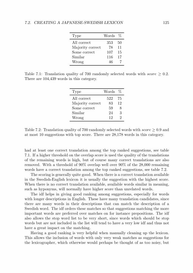
7.2. CREATING A JAPANESE-SWEDISH LEXICON 125
Type Words %
All correct 353 50Majority correct 78 11Some correct 107 15Similar 116 17Wrong 46 7
Table 7.1: Translation quality of 700 randomly selected words with score ≥ 0.2.There are 104,439 words in this category.
Type Words %
All correct 522 75Majority correct 83 12Some correct 59 8Similar 24 3Wrong 12 2
Table 7.2: Translation quality of 700 randomly selected words with score ≥ 0.9 andat most 10 suggestions with top score. There are 28,178 words in this category.
had at least one correct translation among the top ranked suggestions, see table7.1. If a higher threshold on the overlap score is used the quality of the translationsof the remaining words is high, but of course many correct translations are alsoremoved. With a threshold of 90% overlap well over 90% of the 28,000 remainingwords have a correct translation among the top ranked suggestions, see table 7.2.
The scoring is generally quite good. When there is a correct translation availablein the Swedish-English lexicon it is usually the suggestion with the highest score.When there is no correct translation available, available words similar in meaning,such as hyponyms, will normally have higher score than unrelated words.
The idf helps in giving good ranking among suggestions, especially for wordswith longer descriptions in English. These have many translation candidates, sincethere are many words in their descriptions that can match the description of aSwedish word. The idf orders these matches so that suggestions matching the moreimportant words are preferred over matches on for instance prepositions. The idfalso allows the stop word list to be very short, since words which should be stopwords but are not included in the list will tend to have a very low idf and thus nothave a great impact on the matching.
Having a good ranking is very helpful when manually cleaning up the lexicon.This allows the inclusion of words with only very weak matches as suggestions forthe lexicographer, which otherwise would perhaps be thought of as too noisy, but

126 CHAPTER 7. BILINGUAL LEXICONS
Type Words %
All correct 622 89Majority correct 38 5Some correct 21 3Similar 9 1Wrong 10 1
Table 7.3: Translation quality of 700 randomly selected words with score = 1.There are 16,843 words in this category.
still includes many words with correct translations.Allowing word pairs as translations increases the number of correct translations
drastically. The EDICT includes many words which have no direct translation inSwedish, at least not one that is available in the other lexicon. The coverage thuswould be very low using just a one to one matching of the index terms from thetwo lexicons. Of course, there are also some words and expressions in EDICT thatwould require more than two of the available Swedish index terms.
Since it is generally better to have a match on one entry in the Swedish-Englishlexicon than on two, the ranking score of pairs was reduced by 5%. During theevaluation it was found that it might be better to reduce them even further, perhapsas much as 25%. Examples where this would be better include many colors, suchas “light green” which is translated as “light” + “green”, with perfect overlapfrom a pair of Swedish words. While this is quite good it is not as good as theSwedish word for light green, which is available. The reason this does not rankhigher is that the Swedish word is translated as “light or pale green”, thus onlyscoring 76% overlap. Then again, “heavyweight” also scores 76% as a translationfor “light heavyweight” and would thus replace the current translation “light” +“heavyweight”, but a better value than 5% could likely be found.
Finally, here is a simple example of the impact of the ranking methods: Theword “horoyoi” is translated as “slightly drunk, tipsy” in the Japanese-Englishlexicon. Since no Swedish word has this exact translation, there are only partialmatches. The top scoring matches are all Swedish words for drunk or tipsy, rankedas 52% overlap (matching “tipsy”). Next comes the Swedish word for “slightly”,with 50% overlap. This is followed by more Swedish words matching “drunk”.When allowing pairs of words to match one word, the top suggestions all consist of“slightly” and different words for “drunk”, with an overlap of 76%.
One possible improvement is checking the word class of suggestions, mostlydisambiguating between the noun and verb sense of many English words. Manyerroneous translations include the related verb form for a noun and vice versa.
Another problem is that the Japanese-English lexicon uses American spelling(e.g. “honor”) while the Swedish-English lexicon uses British spelling (e.g. “hon-

7.3. CREATING A THAI-SWEDISH LEXICON 127
our”). Harmonizing the spelling would give better translations, since currentlysome words that should match will not be considered equal.
It would also be nice to use other intermediate languages to improve the qualityof the translations, but there was no other language with sufficiently large lexiconsavailable. Mainly this bottleneck was on the Swedish side; for Japanese thereare other quite large lexicons available. The smaller available lexicons for otherlanguages could likely be used to improve the quality for the covered vocabulary,though.
The method is of course not limited to generating a Japanese-Swedish lexicon.Using the same source lexicons a Swedish-Japanese lexicon could also be generated,and in fact it has been done. The reason this lexicon was not evaluated in the sameway was that the people available for evaluating the lexicon were not very proficientin Japanese. The quality could be assumed to be similar to the Japanese-Swedishlexicon, though.
The highest quality translations have been made available on the Internet, athttp://www.japanska.se, were manual improvement of the lexicon has also beendone. Other parts of the results are available on request.
7.3 Creating a Thai-Swedish Lexicon
The same method that was used in the previous section was later used to generatea Thai-Swedish lexicon. There were a few modifications of the method, namely:one source language word was only allowed to be translated by one target languageword; words explicitly marked as a certain word class was not allowed to matchwords explicitly marked as some other word class.
The created lexicon consists of over 20,000 words, which is the largest Swedish-Thai lexicon known to us. The next largest machine searchable lexicon knowncontains about 2,000 words, though in book form there are lexicons of about 7,000words available. The main drawback of the automatically created lexicon is ofcourse that it contains erroneous translations.
For creating the Swedish-Thai lexicon, the Thai-English lexicon Lexitron (Pal-ingoon et al., 2002) was used. It is a freely available dictionary from NECTEC(downloadable from http://www.nectec.or.th/) which includes not only transla-tions but also word class information, example sentences and pronunciation.
7.4 NLP Tools for Lexicon Lookup
The work in this section was developed with helpful suggestions from WanwisaKhanaraksombat, who also did all the evaluations. This section is based on the pa-per “Developing and Evaluating a Searchable Swedish – Thai lexicon” (Khanarak-sombat and Sjöbergh, forthcoming).
A simple web interface for looking up words in the Thai-Swedish lexicon fromthe previous section was created. To help users of the lexicon interface, especially

128 CHAPTER 7. BILINGUAL LEXICONS
learners of Swedish, some language technology tools were added. These includespelling checking, inflection, and compound analysis. These tools were only imple-mented for searches in Swedish. In the spirit of believing that the user is probablyright if the system understands the query, these tools are only used if the searchfails to return any matches.
The first tool is spelling correction. Experiences from other popular lexiconservices on the Internet indicate that a substantial part of all queries are misspelled,even by native speakers. Thus, if a query returns no results, the word is put througha spelling checker. If there are suggested corrections from the spelling checker,all such suggestions are automatically used as search queries and the resultingtranslations are shown.
The second tool is a lemmatizer. When there are no results, the lemma formof the word is used instead, since some word classes have quite rich inflection inSwedish but only the lemma forms are listed in the lexicon.
The third tool is compound splitting, since Swedish has very productive com-pounding. Search queries that return no results can be automatically split intotheir compound components. The translations of each component are presented togive an indication of the meaning of the whole compound.
It is also possible to search the lexicon using words in Thai (or even English),though the language tools only work for Swedish.
Since there is a possibility of erroneous translations, mainly caused by ambigu-ous English words, it is also possible to view the original English translations, colorcoded to show which parts have a matching word in the corresponding translation.Other helpful information, such as sound files with Swedish pronunciation, is alsoavailable.
The Swedish-Thai lexicon and the lexicon tools were evaluated in a small userstudy. Six students, native speakers of Thai currently studying in Sweden, wereasked to use the lexicon while solving some simple tasks. The students have been inSweden one to two years and have been studying Swedish for six to twelve months.
The students, working in pairs, were given the task of creating a short storyfrom eight given pictures. The story was to be written in Swedish, so the lexiconwas mainly used for searching in Thai, to find Swedish words for what the studentswanted to express.
The students were observed while working and after the task was finished aninterview was conducted. Overall, the students thought the lexicon worked well.However, the user interface was confusing, too much information was presented atonce in an unstructured way. Also, too many matches were returned for manysearches, which further increased this problem. This is probably caused by thebilingual lexicon generation method, which stores all translations when there ismore than one possible translation with the same quality, instead of keeping onlythe most appropriate translation.
The most praised point was that the original English translations were alsoavailable, which makes it possible to check whether the translations were likely tobe correct when one is unsure if the Swedish word is the correct one. Despite this it

7.4. NLP TOOLS FOR LEXICON LOOKUP 129
did happen that the students were tricked by erroneous translations in the lexicon.One example is using the word “förmiddag” which indicates times roughly between9 AM and noon, instead of “morgon”, which indicates times roughly between 6 AMand 9 AM.
Suggested improvements include having the user interface available also in Thai,adding more information such as the gender class of Swedish nouns and reducing thenumber of matching translations by removing less common translation possibilities.For most purposes the students would be happy with coverage of only commonwords.
It was also suggested that the options to turn the NLP tools on or off be removedfrom the user interface since the students thought that the tools should always beused. Pronunciation help was not used by the students in these tasks, but theythought that it was a good thing to include in a lexicon. Most students thoughtthat the most difficult part of learning Swedish was the pronunciation. Building alarge vocabulary was also considered hard, while Swedish grammar was not thoughtto be very difficult, mainly because of its similarity to English grammar.
Another user study, were the students are given a Swedish text to translate intoThai, is also planned.


Chapter 8
Automatic Generation of Puns
In this chapter some simple experiments on computational humor are presented.A program that generates puns in Japanese was created and evaluated to test thehypothesis that by using “bad words” jokes become a little bit more funny. Thischapter is based on the paper “Vulgarities are fucking funny, or at least make thingsa little bit funnier” (Sjöbergh, forthcomingb). Thanks must go to all the peoplewho participated in the evaluations of the jokes, and especially to Kanko Uchimuraand Mitsukazu Tabuchi who gave very thorough comments.
There have been some attempts at creating puns in Japanese before (Yokogawa,2001, Binsted and Takizawa, 1998). In (Binsted and Takizawa, 1998) a system forgenerating punning riddles in Japanese is described. The program of this chapterwas developed in a very similar way. The big difference being the use of “badwords” to hopefully make the generated puns a little funnier. Two different kindsof jokes were generated, riddles using puns and proverbs changed in a pun-like wayto new expressions.
8.1 Preliminary Test: Punning Riddles
A very simple program for generating riddles was created. When generating pun-ning riddles, three connected words are searched for and then inserted into a fixedtemplate. This template is “An X is an X but what kind of X is Y? Z!”. HereX and Z are two words that have similar pronunciation. Y is a description thatmatches the meaning of Z. To make things funnier, Z is always chosen from a listof vulgar or taboo words. This list was constructed for this program, with wordscollected from different sources.
An example joke (freely translated into English) generated by the program is:“Sisters (shimai) are sisters, but what kind of sisters are untidy? Sloppy bitches(darashinai).”
X and Z are found by looking through a dictionary of words, checking all wordpairs to see how similar the pronunciation is. Similarity is based on a few simple
131

132 CHAPTER 8. AUTOMATIC GENERATION OF PUNS
Sound Similarity
i, e 0.7u, o 0.7a, other vowel 0.55V 1, V 2 0.5n, m 0.9g, b, d 0.9k, p, t 0.9kiV , kiyV 0.95kiV , kyV 0.9kiyV , kyV 0.9V , yV 0.7shi, hi 0.95voiced/unvoiced (z-s, d-t, g-k, . . . ) 0.7
Table 8.1: Pronunciation similarity scores used. V indicates a vowel sound.
rules for which sounds are similar in Japanese. Similarity scores used are shown intable 8.1.
When Z has been selected, the description Y is generated by looking in a dic-tionary of Japanese, with descriptions of the words also written in Japanese. TheSanseido online dictionary was used for this. If the first sentence in the descriptionis short, the whole sentence is used as Y. Otherwise the first word of the sentenceis used.
Since the joke is not funny if X and Z are synonyms, a check is also done tosee if the meanings are too similar. This is done by checking the word overlap ofthe English descriptions of X and Z in a Japanese-English dictionary, for which theEDICT (Breen, 1995) was used.
A very small evaluation of this program was done by letting four Japanesereaders read jokes and decide how funny they were on a scale from 1 (not funny) to5 (very funny). It was also possible to select “I don’t understand” if for some reasonit was impossible to tell if the joke was funny or not; for instance if it containeddifficult words that the reader did not understand.
The evaluation contained 5 examples of similar (though not vulgar) jokes cre-ated by humans, found on the Internet. There were also 10 non-jokes, created byselecting X, Y and Z by randomly drawing words from the dictionary. Finally therewere 15 jokes from the program described above and another 15 jokes generatednot using the vulgar words (i.e. Z was selected as a similar sounding word from thenormal word list).
The reason that the evaluation was very small was that the jokes were consideredalmost completely unfunny by most readers. All readers did give vulgar jokes higherscores than non-vulgar jokes, though, and most readers gave human generated jokes
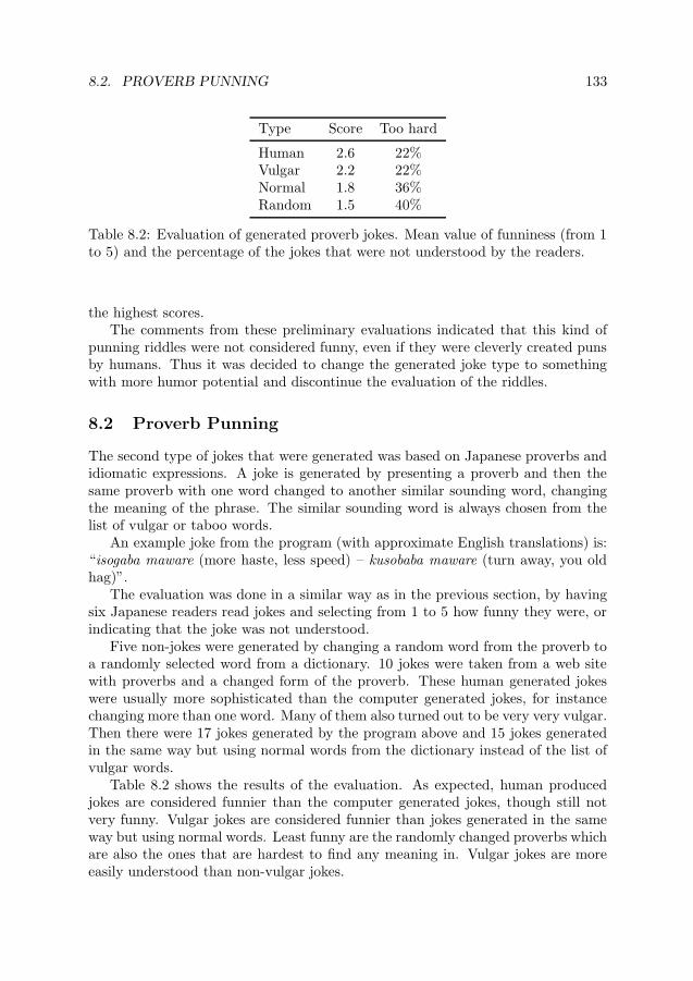
8.2. PROVERB PUNNING 133
Type Score Too hard
Human 2.6 22%Vulgar 2.2 22%Normal 1.8 36%Random 1.5 40%
Table 8.2: Evaluation of generated proverb jokes. Mean value of funniness (from 1to 5) and the percentage of the jokes that were not understood by the readers.
the highest scores.The comments from these preliminary evaluations indicated that this kind of
punning riddles were not considered funny, even if they were cleverly created punsby humans. Thus it was decided to change the generated joke type to somethingwith more humor potential and discontinue the evaluation of the riddles.
8.2 Proverb Punning
The second type of jokes that were generated was based on Japanese proverbs andidiomatic expressions. A joke is generated by presenting a proverb and then thesame proverb with one word changed to another similar sounding word, changingthe meaning of the phrase. The similar sounding word is always chosen from thelist of vulgar or taboo words.
An example joke from the program (with approximate English translations) is:“isogaba maware (more haste, less speed) – kusobaba maware (turn away, you oldhag)”.
The evaluation was done in a similar way as in the previous section, by havingsix Japanese readers read jokes and selecting from 1 to 5 how funny they were, orindicating that the joke was not understood.
Five non-jokes were generated by changing a random word from the proverb toa randomly selected word from a dictionary. 10 jokes were taken from a web sitewith proverbs and a changed form of the proverb. These human generated jokeswere usually more sophisticated than the computer generated jokes, for instancechanging more than one word. Many of them also turned out to be very very vulgar.Then there were 17 jokes generated by the program above and 15 jokes generatedin the same way but using normal words from the dictionary instead of the list ofvulgar words.
Table 8.2 shows the results of the evaluation. As expected, human producedjokes are considered funnier than the computer generated jokes, though still notvery funny. Vulgar jokes are considered funnier than jokes generated in the sameway but using normal words. Least funny are the randomly changed proverbs whichare also the ones that are hardest to find any meaning in. Vulgar jokes are moreeasily understood than non-vulgar jokes.

134 CHAPTER 8. AUTOMATIC GENERATION OF PUNS
8.3 Discussion
The generated jokes were not considered very funny, most jokes scored the lowestpossible value of one. Jokes by humans also scored very low. The scores variedquite a lot between different readers, though, with one reader assigning a meanscore of 4.1 and another 1.2.
Many jokes were hard to understand. This was caused by among other thingsusing proverbs that the reader was not familiar with, using slang words or difficultwords that the reader did not know, writing otherwise known words using difficultkanji that reader did not understand and similar things. There were also somemistakes in the automatic assignment of pronunciation to some words written withkanji, which was confusing.
Many jokes were also incomprehensible for the simple reason that the new worddid not make any sense in the changed proverb, so it was impossible to construe areasonable meaning for the new phrase. This was less of a problem with the vulgarwords than other words, likely because the vulgar words have many meanings orcan be used in many ways.
The readers also had the possibility to write any comment they liked aboutthe jokes. One comment was that some jokes were cleverly created but too vulgaror offensive, so the total funniness was low, at least for this reader. This usuallyreferred to the human generated jokes.
Other comments included things like stating that a certain joke was not funny,but with a very small change to another word too, it would be much funnier. Thisindicates that it is probably a good idea to change more than one word, selectingseveral new words that are related to each other.
8.4 Conclusions
The theory that bad words are funny seems to hold for the generated jokes. Whenusing bad words, it also seems to be easier to find a reasonable interpretation ofthe new generated proverb. While the generated jokes were not considered veryfunny in general, neither were the jokes generated by humans. There were someautomatically generated jokes that were considered quite funny by most readers.
Future possibilities include changing the proverbs in more sophisticated ways,by for instance selecting words that have a meaning related to the remaining wordsin the proverb, by changing more than one word in each proverb, by changingwords to words without similar pronunciation but with related meanings (such asantonyms) etc. Another possibility is to generate puns on other types of texts, suchas titles of famous movies or books.
Generating jokes that are funny regardless of context, such as these jokes haveto be since they have no context, is quite hard. Another possibility is to generatejokes in a certain context, which then can be used. A simple example would be adialogue system, were the previous sentences can be used as a context to base jokes
8.4. CONCLUSIONS 135
on. While in general it is easier to produce jokes that are funny in a certain contextthan jokes that are always funny, understanding how to use the context to make afunny joke is of course a quite hard problem.


Chapter 9
Contributions and FutureThoughts
In this thesis, different methods for processing natural languages were presented.The common theme was to avoid manual work as much as possible, instead havingthe computer perform the work.
The first part of the thesis presented methods that are useful in many languageprocessing situations. The first example was part of speech tagging, an importanttool in many applications. How to improve the tagging accuracy without usingany extra manual work, by combining different automatic systems, was discussed.Effects of the quality and genre of the training data were also examined, showingthat text quality was perhaps surprisingly unimportant and that quite good resultscan be achieved without explicitly using manual annotation. Combining manuallyannotated data and automatically annotated data lead to better results than us-ing either resource alone. Finally, a new method for part of speech tagging waspresented. While not very good on its own, it was useful in combination with othersystems.
When it comes to combining systems for tagging, it would be interesting tofurther explore more sophisticated methods that can take dependencies among thefeatures into account. A method that could for instance discover that when theStomp tagger is very confident, it is almost always right so we can ignore the outputof the other systems, but when it is less sure the performance is not as impressive.
For the Stomp part of speech tagger, it would be interesting to evaluate theperformance using a much larger training corpus. Using only a one million wordscorpus gives quite sparse data for Stomp, compared to the information used byother systems. This means that it is likely that the improvement gained by using alarger training corpus is greater for Stomp than for the systems that outperformedStomp using the smaller resource.
Also regarding training data, it would be interesting to examine the impactof adding texts with syntactic errors to the training data. In grammar checking
137

138 CHAPTER 9. CONTRIBUTIONS AND FUTURE THOUGHTS
applications the part of speech tagger usually plays a very important role. Thetagger is however normally only trained on more or less error free texts. This meansthat the tagger often hides errors in the text by finding a grammatical but veryunlikely interpretation of the sentence, ignoring the correct interpretation since forthe tagger the likelihood of an erroneous sentence is basically zero. Having errors inthe training data would increase the likelihood of erroneous sentences as viewed bythe tagger, which might give more useful tagging results for the grammar checker.
Next in the first part of the thesis, compound splitting by statistical means wasexamined. Many different methods were evaluated, and as expected a combinationof several methods performs much better than any single method. It was shownthat using only quite meager resources, good results can be achieved using statisticalmethods. In the future, it would be interesting to see how well the methods mightperform if larger training resources were available. Evaluating these methods onother languages were compounding is common would also be interesting.
The last chapter in the first half of the thesis dealt with evaluation methods.Evaluating language tools is very important, since because languages are relativelyvaguely defined, it is hard to prove if a system works, so evaluations are the onlyway to see if a system actually seems to perform well. The evaluation methodspresented show how resources annotated for one purpose, here parsing, can be usedto evaluate a different aspect of a system than first expected. The robustness of aparsing system can be evaluated even if the annotated resource only contains errorfree text. It was also shown how some information on the robustness of a systemcan be calculated using no annotated resources at all.
The unsupervised estimates can most likely be improved, since the currentmethod tends to give an interval were accurate systems are usually found in oneend and less accurate systems in the other end of the interval. Adjusting the guessof where in the interval the true accuracy lies to take this into account should bepossible. It would also be interesting to apply the same kind of reasoning to developunsupervised evaluation methods for other types of language processing tasks.
In the second part of the thesis some useful applications of language processingwere presented. The first of these was grammar checking, which many people useevery day. The work presented showed statistical methods for detecting errorsin text. These generally complement traditional grammar checking methods us-ing manually constructed error detection rules. Statistical methods usually detectthings that differ from a normative training resource, while manual methods lookfor specific erroneous constructions.
One of the strengths of the statistical methods is that they are good at findingerrors that no one imagined people could make, which is hard to capture by writingrules. The same ability also leads to false alarms, when a new genre is examinedand grammatical constructions that are common in the new genre but rare in thenormative training data are discovered.
In the future, it would be interesting to do work on how to present a useful errordiagnosis and possible suggestions for corrections when a statistical method findsa suspected error. It would also be interesting to modify the methods that report

139
that a certain construction is rare enough in the training data to be suspicious innew text. A modified version could then signal that a certain construction is verycommon in correct text, but lacking in the current text. This kind of avoidance ofcertain language constructions is common among learners of a new language, butcurrent tools generally ignore this type of error.
The second chapter in the second half of the thesis presented two new methodsfor automatic summarization. One tries to evaluate the whole summary at once,calculating how similar it is in content to the original text. This method givessummaries that try to capture all the content of the original text, while some othersystems focus on finding one important topic and reporting mainly on this. Thesecond method presented tries to produce extractive summaries that have smoothertransitions between sentences than other methods. Both methods require only quiteunsophisticated tools, such as sentence and word boundary detection.
In the future, these methods could be improved by using more sophisticatedtools, for instance for anaphora resolution or for removal of uninteresting parts ofsentences. It would also be interesting to evaluate them on other languages, sinceboth methods can easily be adapted to many other languages.
A method for automatically generating a bilingual dictionary using dictionar-ies to a common intermediate language was also presented. This method had twoslight modifications to the more or less standard way to do this. Both modificationswere meant to improve the recall of the resulting dictionary, possibly at the cost oftranslation quality. This resulted in two new large bilingual dictionaries, betweenSwedish and Japanese and Swedish and Thai. A dictionary search interface in-cluding some language tools to help writers lacking a perfect grasp of the sourcelanguage was also produced.
Work is now performed on increasing the quality of these dictionaries, mostly bymanually cleaning out bad translations. It would also be interesting to use severalintermediate languages instead of only one, which removes many of the problemsleading to bad translations.
Finally, some simple experiments on generating jokes automatically were presen-ted. While the results were not very impressive, the theory that by using “badwords” jokes become a little bit more funny seems to hold. While humor may notseem to be very important in the context of computers, it is a very important partof human interaction. Thus, it would probably be useful for instance in humancomputer interaction to have some understanding of humor. While not very muchresearch has been done when it comes to computational humor, some progress hasbeen made. It seems to be an area of research with many interesting possibilities.
To sum up, statistical methods can be useful in many language processing tasks.While better results can often be achieved by using manual work than by using onlystatistics, even better results can often be achieved by using both types of work.


Bibliography
Kamal M. Ali and Michael J. Pazzani. 1996. Error reduction through learningmultiple descriptions. Machine Learning, 24(3):173–202.
Antti Arppe. 2000. Developing a grammar checker for Swedish. In Proceedings ofNodalida ’99, pages 13–27. Trondheim, Norway.
Eric Steven Atwell. 1987. How to detect grammatical errors in a text withoutparsing it. In Proceedings of the 3rd EACL, pages 38–45, Copenhagen, Denmark.
Harald Berthelsen and Beáta Megyesi. 2000. Ensemble of classifiers for noise detec-tion in pos tagged corpora. In Proceedings of the Third International Workshopon TEXT, SPEECH and DIALOGUE, pages 27–32, Brno, Czech Republic.
Johnny Bigert. 2005a. Automatic and Unsupervised Methods in Natural LanguageProcessing. PhD thesis, KTH, Stockholm, Sweden.
Johnny Bigert. 2005b. Unsupervised evaluation of Swedish spell checker correctionsuggestions. In Proceedings of Nodalida 2005, Joensuu, Finland.
Johnny Bigert, Linus Ericson, and Antoine Solis. 2003a. Missplel and AutoEval:Two generic tools for automatic evaluation. In Proceedings of Nodalida 2003,Reykjavik, Iceland.
Johnny Bigert, Viggo Kann, Ola Knutsson, and Jonas Sjöbergh. 2004. Grammarchecking for Swedish second language learners. In Peter Juel Henrichsen, editor,CALL for the Nordic Languages, pages 33–47. Samfundslitteratur.
Johnny Bigert and Ola Knutsson. 2002. Robust error detection: A hybrid approachcombining unsupervised error detection and linguistic knowledge. In Proceedingsof Romand 2002, Robust Methods in Analysis of Natural Language Data, pages10–19, Frascati, Italy.
Johnny Bigert, Ola Knutsson, and Jonas Sjöbergh. 2003b. Automatic evaluation ofrobustness and degradation in tagging and parsing. In Proceedings of RANLP-2003, pages 51–57, Borovets, Bulgaria.
141
142 BIBLIOGRAPHY
Johnny Bigert, Jonas Sjöbergh, Ola Knutsson, and Magnus Sahlgren. 2005. Unsu-pervised evaluation of parser robustness. In Proceedings of CICling 2005, pages142–154, Mexico City, Mexico.
Kim Binsted and Osamu Takizawa. 1998. BOKE: A Japanese punning riddle gen-erator. Journal of the Japanese Society for Artificial Intelligence, 13(6):920–927.
Juhani Birn. 2000. Detecting grammar errors with Lingsoft’s Swedish grammarchecker. In Proceedings of Nodalida ’99, pages 28–40. Trondheim, Norway.
Igor Bolshakov. 2005. An experiment in detection and correction of malapropismsthrough the web. In Proceedings of CICling 2005, pages 803–815, Mexico City,Mexico.
Francis Bond, Ruhaida Binti Sulong, Takefumi Yamazaki, and Kentaro Ogura.2001. Design and construction of a machine-tractable Japanese-Malay dictionary.In Proceedings of MT Summit VIII, pages 53–58, Santiago de Compostela, Spain.
Lars Borin. 2000. Something borrowed, something blue: Rule-based combination ofPOS taggers. In Proceedings of the Second International Conference on LanguageResources and Evaluation, pages 21–26, Athens.
Thorsten Brants. 2000. TnT – a statistical part-of-speech tagger. In Proceedings ofthe 6th Applied NLP Conference, ANLP-2000, pages 224–231, Seattle, USA.
Jim Breen. 1995. Building an electronic Japanese-English dictionary. In JapaneseStudies Association of Australia Conference, Brisbane, Australia.
Eric Brill and Jun Wu. 1998. Classifier combination for improved lexical disambig-uation. In Proceedings of COLING-ACL’98, pages 191–195, Montreal, Canada.
Jaime G. Carbonell and Jade Goldstein. 1998. The Use of MMR, Diversity-BasedReranking for Reordering Documents and Producing Summaries. In AlistairMoffat and Justin Zobel, editors, SIGIR98, pages 335–336, Melbourne, Australia.
Johan Carlberger and Viggo Kann. 1999. Implementing an efficient part-of-speechtagger. Software – Practice and Experience, 29(9):815–832.
John Carroll, Ted Briscoe, and Antonio Sanfilippo. 1998. Parser evaluation: asurvey and a new proposal. In Proceedings of the 1st International Conferenceon Language Resources and Evaluation LREC 1998, pages 447–454, Granada,Spain.
Martin Chodorow and Claudia Leacock. 2000. An unsupervised method for detect-ing grammatical errors. In Proceedings of NAACL’00, pages 140–147, Seattle,USA.

143
Walter Daelemans, Jakub Zavrel, Peter Berck, and Steven Gillis. 1996. MBT:A MemoryBased part of speech tagger-generator. In Proceedings of the FourthWorkshop on Very Large Corpora, pages 14–27, Copenhagen, Denmark.
Walter Daelemans, Jakub Zavrel, Ko van der Sloot, and Antal van den Bosch. 2001.Timbl: Tilburg memory-based learner – version 4.0 reference guide.
Hercules Dalianis. 2002. Evaluating a spelling support in a search engine. InProceedings of NLDB 2002, pages 183–190, Stockholm, Sweden.
Hercules Dalianis. 2005. Improving search engine retrieval using a compound split-ter for Swedish. In Proceedings of Nodalida 2005, Joensuu, Finland.
Thomas Dietterich. 1997. Machine learning research: Four current directions. AIMagazine, 18(4):97–136.
Richard Domeij, Ola Knutsson, Johan Carlberger, and Viggo Kann. 2000. Granska– an efficient hybrid system for Swedish grammar checking. In Proceedings ofNodalida ’99, pages 49–56, Trondheim, Norway.
Rickard Domeij, Joachim Hollman, and Viggo Kann. 1994. Detection of spellingerrors in Swedish not using a word list en clair. J. Quantitative Linguistics, 1:195–201.
DUC. 2005. Document understanding conferences. http://duc.nist.gov/.
Elżbieta Dura. 1998. Parsing Words. PhD thesis, Göteborg University, Göteborg,Sweden.
H. P. Edmundson. 1969. New Methods in Automatic Extracting. Journal of theAssociation for Computing Machinery, 16(2):264–285.
Jan Einarsson. 1976. Talbankens skriftspråkskonkordans. Lund University.
Eva Ejerhed, Gunnel Källgren, Ola Wennstedt, and Magnus Åström. 1992. Thelinguistic annotation system of the Stockholm-Umeå Corpus project. Technicalreport, Department of General Linguistics, University of Umeå (DGL-UUM-R-33), Umeå, Sweden.
David Elworthy. 1994. Automatic error detection in part of speech tagging. InProceedings of the International Conference on New Methods in Language Pro-cessing, Manchester, UK.
Brian Everitt. 1977. The Analysis of Contingency Tables. Chapman and Hall.
Jennifer Foster. 2004. Parsing ungrammatical input: An evaluation procedure. InProceedings of LREC 2004, pages 2039–2042, Lisbon, Portugal.

144 BIBLIOGRAPHY
Martin Gellerstam, Yvonne Cederholm, and Torgny Rasmark. 2000. The bank ofSwedish. In Proceedings of LREC 2000, pages 329–333, Athens, Greece.
Andrew Golding. 1995. A bayesian hybrid for context sensitive spelling correc-tion. In Proceedings of the 3rd Workshop on Very Large Corpora, pages 39–53,Cambridge, USA.
John Goldsmith. 2001. Unsupervised learning of the morphology of a natural lan-guage. Computational Linguistics, 27(2):153–198.
Linda Van Guilder. 1995. Automated part of speech tagging: A brief overview.Handout for LING361.
Margaret Hafer and Stephen Weiss. 1974. Word segmentation by letter successorvarieties. Information Storage and Retrieval, 10:371–385.
Björn Hammarberg. 1977. Svenskan i ljuset av invandrares språkfel. Nysvenskastudier, 57:60–73.
Na-Rae Han, Martin Chodorow, and Claudia Leacock. 2004. Detecting errors inenglish article usage with a maximum entropy classifier trained on a large, diversecorpus. In Proceedings of LREC-2004, pages 1625–1628, Lisbon, Portugal.
Daniel Hardt. 2001. Transformation-based learning of Danish grammar correction.In Proceedings of RANLP 2001, Tzigov Chark, Bulgaria.
Zellig Harris. 1955. From phoneme to morpheme. Language, 31:190–222.
Martin Hassel. 2001. Internet as corpus - automatic construction of a Swedish newscorpus. In Proceedings of Nodalida 2001, Uppsala, Sweden.
Martin Hassel and Hercules Dalianis. 2005. Generation of reference summaries.In Proceedings of 2nd Language and Technology Conference: Human LanguageTechnologies as a Challenge for Computer Science and Linguistics, pages 21–23,Poznan, Poland.
Martin Hassel and Jonas Sjöbergh. 2005. A reflection of the whole picture is notalways what you want, but that is what we give you. In "Crossing Barriers inText Summarization Research" workshop at RANLP’05, Borovets, Bulgaria.
Martin Hassel and Jonas Sjöbergh. 2006. Towards holistic summarization: Selectingsummaries, not sentences. In Proceedings of LREC 2006, Genoa, Italy.
Eduard Hovy and Chin Yew Lin. 1999. Automated Text Summarization in SUM-MARIST. In Inderjeet Mani and Mark T. Maybury, editors, Advances in Auto-matic Text Summarization, pages 81–94. The MIT Press.

145
Emi Izumi, Kiyotaka Uchimoto, Toyomi Saiga, Thepchai Supnithi, and HitoshiIsahara. 2003. Automatic error detection in the Japanese learners’ English spokendata. In Companion Volume to the Proceedings of ACL ’03, pages 145–148,Sapporo, Japan.
Hongyan Jing. 2000. Sentence Reduction for Automatic Text Summarization. InProceedings of the 6th Applied Natural Language Processing Conference, pages310–315, Seattle, Washington.
Hongyan Jing and Kathleen R. McKeown. 2000. Cut and Paste-Based Text Sum-marization. In ANLP/NAACL00, pages 178–185, Seattle, Washington.
Janne Bondi Johannessen and Helge Hauglin. 1996. An automatic analysis of Nor-wegian compounds. In Papers from the 16th Scandinavian Conference of Lin-guistics, pages 209–220, Turku / Åbo, Finland.
Gunnel Källgren. 1996. Linguistic indeterminacy as a source of errors in tagging.In Proceedings of COLING-96, pages 676–680, Copenhagen, Denmark.
Viggo Kann, Rickard Domeij, Joachim Hollman, and Mikael Tillenius. 2001. Im-plementation aspects and applications of a spelling correction algorithm. InL. Uhlirova, G. Wimmer, G. Altmann, and R. Koehler, editors, Text as a Lin-guistic Paradigm: Levels, Constituents, Constructs. Festschrift in honour ofLudek Hrebicek, volume 60 of Quantitative Linguistics, pages 108–123. WVT,Trier, Germany.
Fred Karlsson. 1992. SWETWOL: A comprehensive morphological analyser forSwedish. Nordic Journal of Linguistics, 15(1):1–45.
Lauri Karttunen, Jean-Pierre Chanod, Gregory Grefenstette, and Anne Schiller.1966. Regular expressions for language engineering. Natural Language Engineer-ing, 2(4):305–328.
Frank Keller and Mirella Lapata. 2003. Using the web to obtain frequencies forunseen bigrams. Computational Linguistics, 29(3):459–484.
Wanwisa Khanaraksombat and Jonas Sjöbergh. forthcoming. Developing and eval-uating a searchable Swedish – Thai lexicon.
Ola Knutsson, Johnny Bigert, and Viggo Kann. 2003. A robust shallow parser forSwedish. In Proceedings of Nodalida 2003, Reykjavik, Iceland.
Philipp Koehn and Kevin Knight. 2001. Knowledge sources for word-level transla-tion models. In Proceedings of EMNLP 2001, Pittsburgh, USA.
Philipp Koehn and Kevin Knight. 2003. Empirical methods for compound splitting.In Proceedings of EACL 2003, Budapest, Hungary.

146 BIBLIOGRAPHY
Dimitrios Kokkinakis and Sofie Johansson Kokkinakis. 1999. Sense-tagging at thecycle-level using GLDB. Technical Report GU-ISS-99-4, Department of Swedish,Göteborg University.
Igor Kononenko. 1994. Estimating attributes: Analysis and extensions of RELIEF.In Proceedings of the European Conference on Machine Learning, pages 171–182,Catania, Italy.
Kimmo Koskenniemi. 1983. Two-level morphology: a general computational modelfor word-form recognition and production. Technical Report 11, Department ofGeneral Linguistics, University of Helsinki.
Sandra Kubler. 2005. Memory based parsing. Computational Linguistics, 31(3):419–421.
Thomas K. Landauer, Peter W. Foltz, and Darrell Laham. 1998. Introduction toLatent Semantic Analysis. Discourse Processes, 25:259–284.
Xin Li and Dan Roth. 2001. Exploring evidence for shallow parsing. In Proceedingsof CoNLL-2001, pages 38–44, Toulouse, France.
Chin-Yew Lin. 2003. ROUGE: Recall-oriented understudy for gisting evaluation.http://www.isi.edu/˜cyl/ROUGE/.
Chin-Yew Lin and Eduard Hovy. 2002. Manual and automatic evaluation of sum-maries. In Proceedings of the Workshop on Automatic Summarization, ACL-2002,pages 45–51, Philadelphia, USA.
Chin-Yew Lin and Eduard Hovy. 2003a. Automatic Evaluation of Summaries UsingN-gram Co-occurrence Statistics. In Proceedings of the 2003 Human LanguageTechnology Conference (HLT-NAACL 2003), Edmonton, Canada.
Chin-Yew Lin and Eduard Hovy. 2003b. The potential and limitations of automaticsentence extraction for summarization. In HLT-NAACL 2003 Workshop: TextSummarization (DUC03), Edmonton, Canada.
Janne Lindberg and Gunnar Eriksson. 2004. CrossCheck-korpusen – en elektronisksvensk inlärarkorpus. In Proceedings of ASLA 2004, Stockholm, Sweden.
Hans Peter Luhn. 1958. The Automatic Creation of Literature Abstracts. IBMJournal of Research Development, 2(2):159–165.
Lidia Mangu and Eric Brill. 1997. Automatic rule acquisition for spelling correction.In Proceedings of the 14th International Conference on Machine Learning, pages187–194, Nashville, USA.

147
Lluís Màrquez, Lluís Padró, and Horacio Rodríguez. 1998. Improving tagging accur-acy by using voting taggers. In Proceedings of the Second Conference on NaturalLanguage Processing and Industrial Applications, NLP+IA/TAL+AI’98, Monc-ton, New Brunswick, Canada.
Lluís Màrquez, Horacio Rodríguez, Josep Carmona, and Josep Montolio. 1999.Improving POS tagging using machine–learning techniques. In Proceedings ofEMNLP/VLC’99, Maryland, USA.
Daniel McDonald and Hsinchun Chen. 2002. Using Sentence Selection Heuristics toRank Text Segments in TXTRACTOR. In Proceedings of the 2nd ACM/IEEEJoint Conference on Digital Libraries, pages 25–38, Portland, Oregon.
Beáta Megyesi. 2001. Comparing data-driven learning algorithms for POS taggingof Swedish. In Proceedings of EMNLP 2001, pages 151–158, Pittsburgh, USA.
Wolfgang Menzel. 1995. Robust processing of natural language. In Proceedingsof the 19th Annual German Conference on Artificial Intelligence, pages 19–34,Berlin, Germany.
Fien De Meulder and Walter Daelemans. 2003. Memory-based named entity re-cognition using unannotated data. In Proceedings of the Seventh Conference onNatural Language Learning, pages 208–211, Edmonton, Canada.
Rada Mihalcea. 2004. Graph-based ranking algorithms for sentence extraction,applied to text summarization. In The Companion Volume to the Proceedingsof 42st Annual Meeting of the Association for Computational Linguistics, pages170–173, Barcelona, Spain.
Joaquim Moré, Salvador Climent, and Antoni Oliver. 2004. A grammar and stylechecker based on internet searches. In Proceedings of LREC-2004, pages 1931–1934, Lisbon, Portugal.
NE. 2000. Nationalencyklopedin. NE Nationalencyklopedin AB.
Grace Ngai and Radu Florian. 2001. Transformation-based learning in the fast lane.In Proceedings of NAACL-2001, pages 40–47, Pittsburgh, USA.
Joakim Nivre. 2003. An efficient algorithm for projective dependency parsing. InProceedings of IWPT 2003, pages 149–160, Nancy, France.
Joakim Nivre, Johan Hall, and Jens Nilsson. 2004. Memory-based dependencyparsing. In Proceedings of CoNLL, Boston, MA.
M. Ortuño, P. Carpena, P. Bernaola-Galván, E. Muñoz, and A. M. Somoza. 2002.Keyword detection in natural languages and DNA. Europhysics Letters, 57(5):759–764.

148 BIBLIOGRAPHY
Paul Over and James Yen. 2004. An introduction to DUC 2004 intrinsic evaluationof generic new text summarization systems.http://www-nlpir.nist.gov/projects/duc/pubs/2004slides/duc2004.intro.pdf.
Kyonghee Paik, Francis Bond, and Shirai Satoshi. 2001. Using multiple pivots toalign Korean and Japanese lexical resources. In Proceedings of NLPRS-2001,pages 63–70, Tokyo, Japan.
Kyonghee Paik, Satoshi Shirai, and Hiromi Nakaiwa. 2004. Automatic con-struction of a transfer dictionary considering directionality. In Proceedings ofMLR2004: PostCOLING Workshop on Multilingual Linguistic Resources, pages31–38, Geneva, Switzerland.
Pornpimon Palingoon, Pornchan Chantanapraiwan, Supranee Theerawattanasuk,Thatsanee Charoenporn, and Virach Sornlertlamvanich. 2002. Qualitative andquantitative approaches in bilingual corpus-based dictionary. In Proceedings ofSNLP-O-COCOSDA 2002, pages 152–158, Hua Hin, Thailand.
Adwait Ratnaparkhi. 1996. A maximum entropy part-of-speech tagger. In Pro-ceedings of the Empirical Methods in Natural Language Processing Conference,Philadelphia, USA.
Magnus Rosell. 2003. Improving clustering of Swedish newspaper articles usingstemming and compound splitting. In Proceedings of Nodalida 2003, Reykjavik,Iceland.
Magnus Sahlgren. 2005. An introduction to Random Indexing. In Methods andApplications of Semantic Indexing Workshop at the 7th International Conferenceon Terminology and Knowledge Engineering, TKE 2005, Copenhagen, Denmark.
Magnus Sahlgren and Rickard Cöster. 2004. Using Bag-of-Concepts to Improve thePerformance of Support Vector Machines in Text Categorization. In Proceedingsof the 20th International Conference on Computational Linguistics, COLING2004, Geneva, Switzerland.
Gerard Salton. 1988. Automatic Text Processing. Addison-Wesley Publishing Com-pany.
SAOL. 1986. Svenska Akademiens ordlista. Elfte upplagan. Svenska Akademien.
Helmut Schmid. 1994. Probabilistic part-of-speech tagging using decision trees.In Proceedings of the International Conference on New Methods in LanguageProcessing, pages 44–49, Manchester, UK.
Satoshi Shirai and Kazuhide Yamamoto. 2001. Linking English words in two bilin-gual dictionaries to generate another language pair dictionary. In Proceedings ofICCPOL-2001, pages 174–179, Seoul, Korea.

149
Satoshi Shirai, Kazuhide Yamamoto, and Kyonghee Paik. 2001. Overlapping con-straints of two step selection to generate a transfer dictionary. In Proceedings ofICSP-2001, pages 731–736, Taejon, Korea.
Jonas Sjöbergh. 2003a. Bootstrapping a free part-of-speech lexicon using a propri-etary corpus. In Proceedings of ICON-2003: International Conference on NaturalLanguage Processing, pages 1–8, Mysore, India.
Jonas Sjöbergh. 2003b. Combining pos-taggers for improved accuracy on Swedishtext. In Proceedings of Nodalida 2003, Reykjavik, Iceland.
Jonas Sjöbergh. 2003c. Stomp, a POS-tagger with a different view. In Proceedingsof RANLP-2003, pages 440–444, Borovets, Bulgaria.
Jonas Sjöbergh. 2005a. Chunking: an unsupervised method to find errors in text.In Proceedings of NODALIDA 2005, Joensuu, Finland.
Jonas Sjöbergh. 2005b. Creating a free digital Japanese-Swedish lexicon. In Pro-ceedings of PACLING 2005, pages 296–300, Tokyo, Japan.
Jonas Sjöbergh. forthcominga. The Internet as a normative corpus: Grammarchecking with a search engine.
Jonas Sjöbergh. forthcomingb. Vulgarities are fucking funny, or at least make thingsa little bit funnier.
Jonas Sjöbergh and Kenji Araki. 2006. Extraction based summarization using ashortest path algorithm. In Proceedings of the 12th Annual Natural LanguageProcessing Conference NLP2006, pages 1071–1074, Yokohama, Japan.
Jonas Sjöbergh and Viggo Kann. 2004. Finding the correct interpretation of Swedishcompounds – a statistical approach. In Proceedings of LREC-2004, pages 899–902, Lisbon, Portugal.
Jonas Sjöbergh and Viggo Kann. 2006. Vad kan statistik avslöja om svenska sam-mansättningar? Språk och Stil, 16.
Jonas Sjöbergh and Ola Knutsson. 2005. Faking errors to avoid making errors:Very weakly supervised learning for error detection in writing. In Proceedings ofRANLP 2005, pages 506–512, Borovets, Bulgaria.
Sylvana Sofkova Hashemi, Robin Cooper, and Robert Andersson. 2003. Positivegrammar checking: A finite state approach. In Proceedings of CICLing-2003,pages 635–646, Mexico City, Mexico.
August Strindberg. 1879. Röda rummet (The Red Room).

150 BIBLIOGRAPHY
Kumiko Tanaka and Kyoji Umemura. 1994. Construction of a bilingual dictionaryintermediated by a third language. In Proceedings of COLING-94, pages 297–303,Kyoto, Japan.
Kagan Tumer and Joydeep Ghosh. 1996. Error correlation and error reduction inensemble classifiers. Connection Science, 8(3–4):385–403.
Hans van Halteren, Jakub Zavrel, and Walter Daelemans. 1998. Improving datadriven wordclass tagging by system combination. In Proceedings of the Thirty-Sixth Annual Meeting of the Association for Computational Linguistics and Sev-enteenth International Conference on Computational Linguistics, pages 491–497,Montreal, Canada.
Hans van Halteren, Jakub Zavrel, and Walter Daelemans. 2001. Improving ac-curacy in word class tagging through combination of machine learning systems.Computational Linguistics, 27(2):99–230.
Qin Iris Wang and Dale Schuurmans. 2005. Improved estimation for unsupervisedpart-of-speech tagging. In Proceedings of the 2005 IEEE International Confer-ence on Natural Language Processing and Knowledge Engineering (IEEE NLP-KE’2005), pages 219–224, Wuhan, China.
David Yarowsky. 1995. Unsupervised word sense disambiguation rivaling super-vised methods. In Proceedings of the 33rd annual meeting on Association forComputational Linguistics, pages 189–196, Morristown, USA.
Toshihiko Yokogawa. 2001. Generation of Japanese puns based on similarity ofarticulation. In Proceedings of IFSA/NAFIPS 2001, Vancouver, Canada.
Juntae Yoon. 2000. Compound noun segmentation based on lexical data extractedfrom corpus. In Proceedings of ANLP 2000, pages 196–203, Seattle, Washington,USA.
Jakub Zavrel, Walter Daelemans, and Jorn Veenstra. 1997. Resolving PP attach-ment ambiguities with memory-based learning. In Proceedings of CoNLL97, pages136–144, Madrid, Spain.