energy characterisation of an aquacultural installation in closed loop

Aquacultural Engineering 21 (1999) 1–18

Energy characterisation of an aquaculturalinstallation in closed loop

Patrick Glouannec, Herve Noel *Laboratoire d’Energetique et de Thermique Industrielle, Uni6ersite de Bretagne Sud,

56325 Lorient, France

Received 22 July 1998; accepted 15 June 1999

Abstract

This article deals with the elaboration of a methodology for the energy characterisation ofan aquacultural plant in closed circuit. A simplified dynamic model representative of thetemperature response of the water volume is defined by identification. The input data are theair temperature, the insolation and the injected power. According to experimental readings,the value of parameters results from the minimisation of a quadratic error criterion betweenthe model output and the water temperature measurements. That model enables the user toquantify the losses and to make energy consumption calculations. In the first place, thestudies carried out on a pilot pond set up on the grounds of the laboratory allowed thetesting of the methodology. Coherent results were first obtained for the open pond and thenfor the pond equipped with a transparent thermal protection. Then, a closed loop designedfor the breeding of turbots was studied. From experimental readings, a model was estab-lished and validated by following the same procedure. © 1999 Elsevier Science B.V. Allrights reserved.

Keywords: Closed loop; Energy characterisation; Thermal model

www.elsevier.nl/locate/aqua-online

Nomenclature

solar recovery area (m2)Aheat capacity (J K−1)Cinsolation (W m−2)Is

fluid conductance (W K−1)Kf

* Corresponding author. Tel.: +33-2978-74515; fax: +33-2978-74517.E-mail address: [email protected] (H. Noel)

0144-8609/99/$ - see front matter © 1999 Elsevier Science B.V. All rights reserved.PII: S0144 -8609 (99 )00017 -5

2 P. Glouannec, H. Noel / Aquacultural Engineering 21 (1999) 1–18

water-air conductance (W K−1)Kw–a

water-ground conductance (W K−1)Kw–gr

heat power (W)Pw

quadratic errorQLaplace’s variablestime (s)t

Ta air temperature (°C)ground temperature (°C)Tgr

water temperature (°C)Tw

y(t) measured outputt time constant (s)

Operators� approximated function

Laplace’s transform�

1. Introduction

The constraints born from the limitation of discharges and the searchfor productivity in intensive aquaculture logically lead to a development ofclosed circuit installations. The low rate of renewal of water in this type ofplant allows the use of heating and/or cooling systems of a moderate size.Moreover, a continuous control of the physio-chemical parameters of watersuch as the temperature, the rate of dissolved oxygen and the pH allows anotable improvement in the development of the species produced. The eco-nomical viability of such an installation requires an understanding of energycosts; this is achieved by accurate sizing and an optimal command of the systemsproducing heat and cold. Two methods can be followed for this purpose. Thefirst one consists in relying on a knowledge based modelling of the phenom-ena of thermal transfer involved, which requires the use of adapted correlationformulae and the knowledge of the thermophysical characteristics of the ma-terials. The second method is based on the identification of parameters representa-tive of the installation under study, which are determined from in situ measure-ments.

The studies, which were carried out on aquacultural installations, first led to thesetting up of thermal behaviour simulation software for a pond of averagedimensions, based on a knowledge based modelling of the different mechanisms ofthermal transfer involved (Noel et al., 1992; Noel, 1993; Noel et al., 1996).This article presents the follow up of this research work and deals with theidentification and the validation of a simplified model representing the thermalresponse of a pond. This linear model allows us to trace back to the staticcharacteristics of the installation and to calculate the heat load in actual operatingconditions.

The methodology was first tested on a pilot experimentation carried out in thelaboratory. Then, extending this work to a closed loop in a turbot breeding facilityvalidated the whole process.

3P. Glouannec, H. Noel / Aquacultural Engineering 21 (1999) 1–18

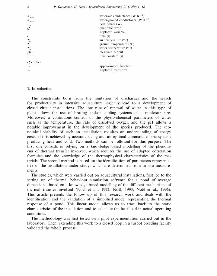
Fig. 1. (a) Characteristics of the experimental pond. (b) Diagram of the hydraulic circuit.


2. Studies on the pilot pond

The pilot fresh water installation is situated near the coast. The pond, whosewalls are of polyurethane and reinforced resin, is buried in sandy soil. The pond hasa hydraulic circuit equipped with thermo-heaters and a heat pump (Fig. 1a and b).An automatic data base acquisition system allows to follow about fifty parameters(weather conditions, temperatures and water level in the pond, ground tempera-tures, flow rates and temperatures in the hydraulic circuit), and to pilot the system.

A model representative of the temperature response of the water volume can beestablished by considering various simplifying hypotheses. The parameters of themodel are then calculated by the minimisation of a quadratic error criterionbetween the calculated response and the measurements. A delayed non-linearprogramming algorithm is used for this calculation.

2.1. Modelling of an open pond

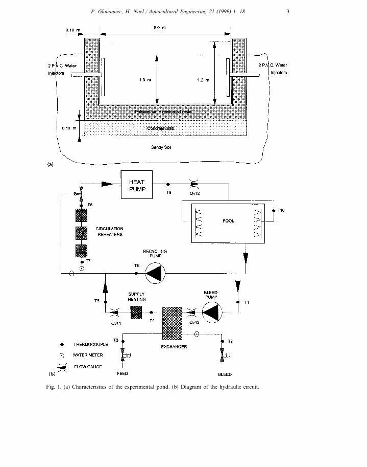
The volume of water is subjected to relatively complex mechanisms of transfer,particularly at the water–air interface (Fig. 2). A simplified thermal model is usedfor the identification. In the case of a first order, an equivalent electrical networkshown on Fig. 3 (Perrin de Brichambaut and Vauge, 1982) represents it. Thetemperature of the volume is assumed to be homogeneous. At the surface of thepond, the convective and long-wave radiative heat exchanges are linearised. Theconductance Kw–a represents all these losses. The mass transfer by evaporation is

Fig. 2. Diagram of thermal exchanges for an open pond.


Fig. 3. Thermal model of a pool (T, temperature; K, conductance; A, solar recovery area; C, heatcapacity).

introduced by a fluid conductance Kf. As the wind conditions have an importantinfluence on the transfers by convection and evaporation, the linearisation of thesetwo mechanisms is the main source of inaccuracy of the model (Klemetson andRogers, 1985; Cathcart and Wheaton, 1987). The solar supplies, depending mainlyon the sun height and the turbidity of the water, are taken into account by meansof the equivalent recuperation area A (De Larminat and Thomas, 1977; Perrin deBrichambaut and Vauge, 1982; Cengel and Ozizik, 1984). Conduction through thewalls is represented by the conductance Kw–gr. The use of the correlations takenfrom literature and selected during our previous studies gave the results presentedin Table 1 (Noel, 1993; Noel et al., 1996). It is worth noting that the losses byconduction with the ground are extremely low, owing to the nature of the walls.They represent approximately 2% of the total losses.

Table 1Characteristic values of the pond determined by correlation formulae with an exchange area of 10 m2

and a water height of 0.90 m

Solar areaConductances Capacity

C (J K−1)Tw=17°C, Ta=7°C Kw–a (W K−1) Kf (W K−1) Turbid water A (m2)relative humidity=70%

Wind speed: 1 m s−1 100 90 December 3.1 37.6×106

5.2June190 200Wind speed: 5 m s−1


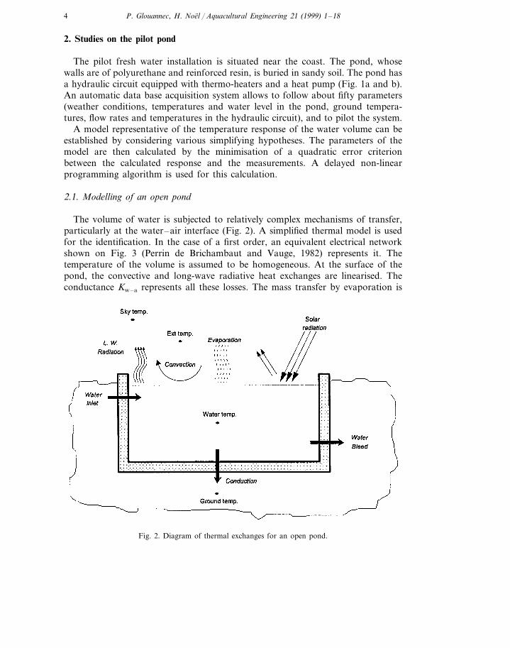
Fig. 4. Picturing of the identification method.

The differential equation of the first order representative of the energy balance isunder the following form:

CdTw

dt=Kw−a(Ta−Tw)+AIs+Pw+Kw−gr(Tgr−Tw)−KfTw (1)

In Laplace’s domain:

T0. w=Tw(0)s+g

+Kw−aT. a+A.I. s+P. w+Kw−grT. gr

Kg(1+ts)(2)

with Tw(0), initial value (°C); Kg, global conductance of losses =Kw–a+Kw–gr+Kf

(W K−1); t, time constant =C/Kg (s); (−g)= (−1/t), pole of the transferfunctions (s−1).

2.2. Identification method

For the delayed identification (De Larminat and Thomas, 1977), the modelmethod is used (Fig. 4). Thanks to the processing of data collections containing avast amount of information (the system being sufficiently prompted), a dynamic,linear model representative of a multi-input and single output system is obtained.The minimisation of error is obtained by an iterative calculation using a gradienttype method far from the solution, and then the Gauss–Newton method toaccelerate the convergence (Marquardt, 1963). The calculation of the modelparameters meets with several difficulties. Within the context of this study, they aremainly due to:� The quasi-stationary ground temperature;� the correlation between the air temperature and the insolation;� the indirect influence of other promptings such as the wind, the hygrometry of

the air…In dynamic operating conditions, the output variable Tw is essentially influenced

by the temperature of the air, the insolation and the power supplied. A model isthus identified as follows:


T0. w=Tw(0)s+g

+g1T( a+g2I( s+g3P( w

1+ts+

Twc

s(3)

with Twc , continual component (°C); Tw(0), initial value (°C), (−g)= (−1/t), pole

of the transfer functions (s−1).The continual component takes into account the promptings that vary little, in

particular the temperature of the ground. By referring to relation (2), we canformulate:

g1=Kw–a/Kg, g2=A/Kg, g3=1/Kg (4)

These parameters, together with the continual component and the initial value,are determined by the minimization of the quadratic error criterion between themodel output and the real system output, that is:

Q= %N

i=1

[T0 w(i)−Tw(i)]2 (5)

where Tw(i ) designates the value measured on the instant t= i Dt (t, time pitch) andN the number of measurements taken. The predicted function values,, are deter-mined by recursive convolution (Semlyen and Dabuleanu, 1976).

Sufficiently long experiments (lasting over 7 days) in appropriate climate condi-tions are required to obtain meaningful results.

The accuracy of the model is quantified by the calculation of the average error:

Qav='Q

N(6)

To assess the relevance of the calculated parameters, several trials are carried outin different conditions: data filtering, variation of the calculation duration.

2.3. Results for the open pond

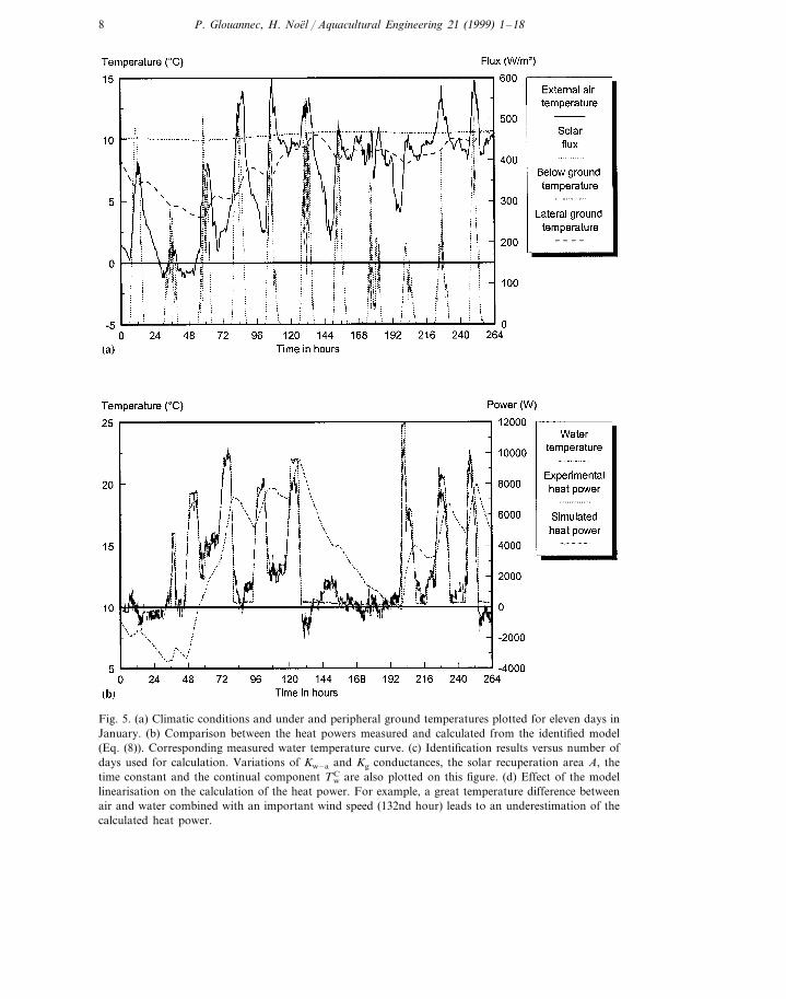
Fig. 5(a and b) present a sequence of measurements taken in the winter period.It can be pointed out that the temperature of the ground under the supportingconcrete slab is almost constant (10°C) in spite of the considerable variations of thewater temperature. The curve of the temperature of the ground near the sidewallsis correlated with the air temperature. The promptings applied to the model, in atime step of 10 min, are the air temperature, the global insolation measuredhorizontally and the heat power supplied to the volume of water. The calculationof this power is made from the recycling flow and the difference between input andoutput water temperature, so that all possible thermal exchanges of the loop arecounted. An intermittent heating was programmed to correctly prompt the system.The calculated values of the model output correspond to the water temperaturesmeasured in various points of the pond. The hypothesis of the homogeneity of thewater temperature is confirmed, since the deviation between the various readingsnever exceeds the precision of the measurements. The continuous recycling of thewater (about 3 m3 h−1) and the use of water injectors limits the water temperaturestratification.


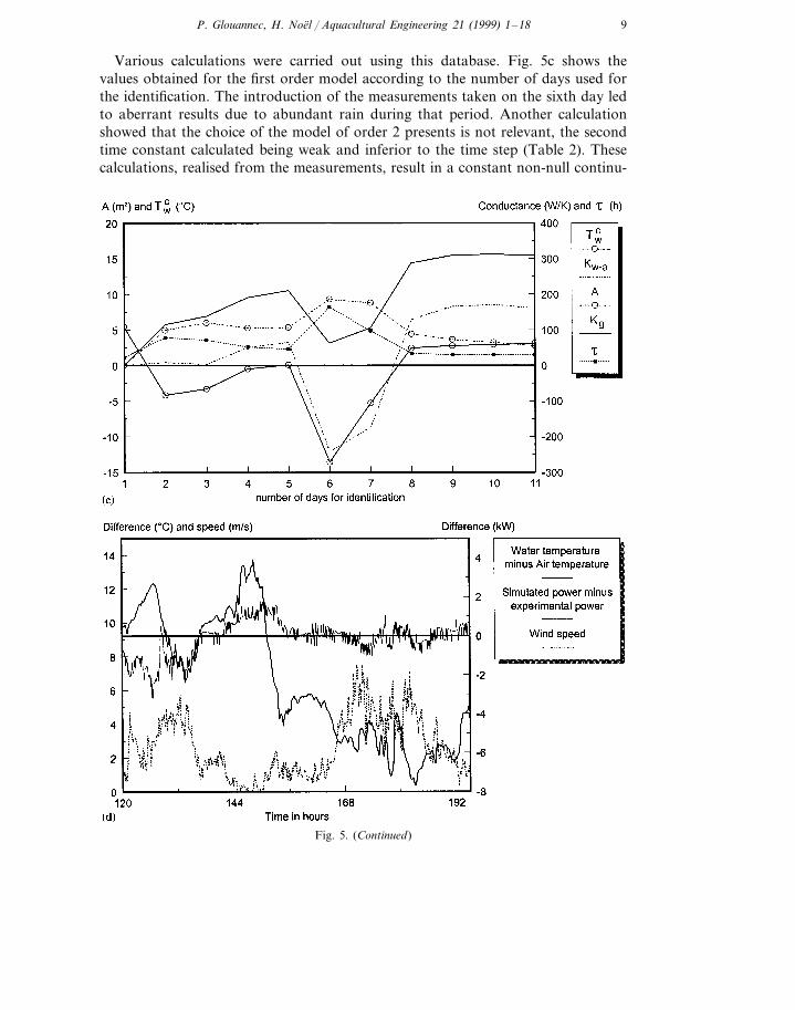
Fig. 5. (a) Climatic conditions and under and peripheral ground temperatures plotted for eleven days inJanuary. (b) Comparison between the heat powers measured and calculated from the identified model(Eq. (8)). Corresponding measured water temperature curve. (c) Identification results versus number ofdays used for calculation. Variations of Kw–a and Kg conductances, the solar recuperation area A, thetime constant and the continual component Tw

C are also plotted on this figure. (d) Effect of the modellinearisation on the calculation of the heat power. For example, a great temperature difference betweenair and water combined with an important wind speed (132nd hour) leads to an underestimation of thecalculated heat power.


Various calculations were carried out using this database. Fig. 5c shows thevalues obtained for the first order model according to the number of days used forthe identification. The introduction of the measurements taken on the sixth day ledto aberrant results due to abundant rain during that period. Another calculationshowed that the choice of the model of order 2 presents is not relevant, the secondtime constant calculated being weak and inferior to the time step (Table 2). Thesecalculations, realised from the measurements, result in a constant non-null continu-

Fig. 5. (Continued)


Table 2Open pond results

Test Order TCw (°C) g1 A (m2) t (h) Kg (W K−1) Qav (°C)Duration (h)

264 2 3.34 0.50 2 38.3 296 0.45a

0.053.09 0.52 2.74 30.7 308 0.50a 264 11.00 0.52 2.75 30.7 308 0.511b 264

a Exploitation of the values measured.b Exploitation of the difference between the values measured and their average values.

ous component a priori due to the influence of the ground. In order to clarify thispoint, a test was carried out by removing the average value from the fourexperimental readings over the period considered. This pre data processing led tothe same model with a weaker constant component.

Concerning the physical consistency of the results, the identification gives valuescorresponding to the previous studies (Table 1), the average wind speed being 2 ms−1 (Fig. 5d). The calculation gives a value of about 300 W K−1 for the globalconductance of loss. The value of g1 (Eq. (3)) shows that the evaporation representsalmost 50% of the losses. A value of 2.7 m2 for the solar area is also a coherentresult in the winter period. Besides, the time constant allows the evaluation of thethermal capacity, that is 34×106 J K−1. Considering the surface of the pond (10m2) and the specific heat of the water, the water level calculated is 0.82 m. Duringthe experiment, the level was maintained at 0.89 m. This relative deviation of 10%is quite acceptable.

In order to validate the results, the simulated and the experimental heat powerare compared. This test is made after passing from the continual model (2) to thenumerical model (De Larminat and Thomas, 1977):

T0 w(i+1)=aT0 w(i)+ (1−a)[g1Ta(i)+g2Is(i)+Pw(i)] (7)

with T0 w(i+1), estimated temperature at instant (i+1)Dt and a=exp(−Dt/t).The following relation gives the power necessary to obtain a reference tempera-

ture in variable weather conditions:

Pw(i)=�Tw(i+1)−aT0 w(i)

1−a−g1Ta(i)=g2Is(i)

n 1g3

(8)

where Tw(i+1) is the required temperature at the instant (i+1)Dt.On Fig. 5b, the power given by the re-heaters is compared to the power

calculated by the Eqs. (7) and (8). For this calculation, we consider the measuredwater temperature as the reference temperature.

The curves are close, except for certain periods. The linearity of the modelidentified inevitably leads to inaccuracies, particularly for the convective andevaporative exchanges. Fig. 5d shows that, according to wind speed, the energyconsumption is over or under estimated, when the difference in temperaturebetween water and air is relatively important.


Fig. 6. (a) Climatic conditions and ground temperature plotted for ten days in February. (b) Comparisonbetween the heat powers measured and calculated from the identified model (Eq. (8)). Correspondingmeasured water temperature and wind speed curves are also plotted. (c) Identification results versusnumber of days used for calculation. Variations of Kg conductance, solar recuperation area A and timeconstant are plotted on this figure.


Fig. 6. (Continued)

3. Impact of a thermal sheeting

For this study, PVC sheeting set on small arches covers the surface of the pond.In this configuration, at the water–air interface, thermal exchanges still occur byevaporation, convection, and long wave radiation. The solar flux must be added tothese losses, since the protection used is a transparent film 500 microns thick.Therefore, a modelling similar to the one previously defined was chosen.

Test sequences carried out over a period of ten days provide the necessarydatabase. The period chosen was quite sunny, with the air temperature undersheeting reaching 30°C on certain days (Fig. 6a and b). Fig. 6c shows the valuesobtained in this configuration.

The experiment shows that the confinement of the water volume facilitates theidentification by a much greater stability of values during calculation (Fig. 6c). Theresults of the various tests, shown in Table 3, emphasise the impact of a transparent

Table 3Results for PVC covered pond

t (h)Duration (h) Kg (W K−1) Qav (°C)Order TCw (°C) g1 A (m2)Test

5.2 73 0.01 155 0.09a 264 2 3.34 0.745.4 73 155 0.111a 3.42264 0.71

1.441 0.11155735.4264 0.71b

a Exploitation of the values measured.b Exploitation of the difference between the values measured and their average values.


thermal protection: the losses are less important (the loss conductance Kg de-creases), the inertia of the system is greater (increase of the time constant t), andthe recuperation of the solar flux is improved (increase of the solar area A).Moreover, the sheeting does not provide full air tightness, but the static gain g1 (Eq.(3)) obtained is closer to unity and shows a limitation of the losses by evaporation.

The curve of the power calculated from the model is shown in Fig. 6b. A verygood consistency between experimentation and calculation can be noted. Since thewind has a lesser influence on the heat exchanges by evaporation and convection atwater–air interface, the hypothesis of the linearity of the model is more justified inthis study than in that of the open pond.

4. Study of an aquacultural plant in closed circuit

4.1. Experiment description

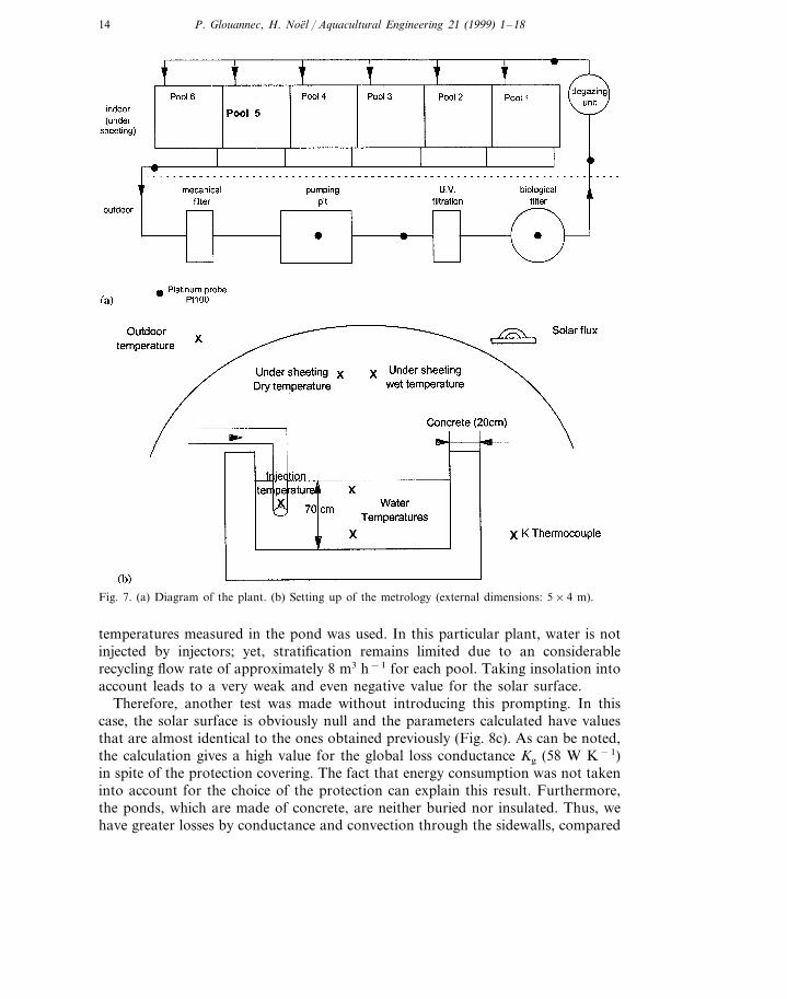
This study describes the characterisation of the thermal behaviour of an aquacul-tural plant functioning in closed circuit and designed for the breeding of turbots.The plant is composed of six ponds supplied in parallel and lying on a concreteslab. The ponds together with water treatment systems, are implanted under atunnel shaped protection (length, 40 m; width, 8 m; height, 3 m) made of a blackporous sheeting (Fig. 7). This plant has functioned in Noirmoutier (France) since1994; the average flow of water changing is of 2 m3 h−1 for a global volume of theloop of 100 m3.

In order to assess the thermal response of the installation, following parameterswere recorded in situ during measuring sequences (Fig. 7):� Temperatures and flow rates at different points of the hydraulic circuit;� water temperatures of the ponds;� air temperature under sheeting (dry and wet temperature);� weather conditions (external air temperature, insolation).

This article presents the procedure followed to establish and validate a modelrepresentative of the thermal behaviour of pool 5.

4.2. Identifying a pool model

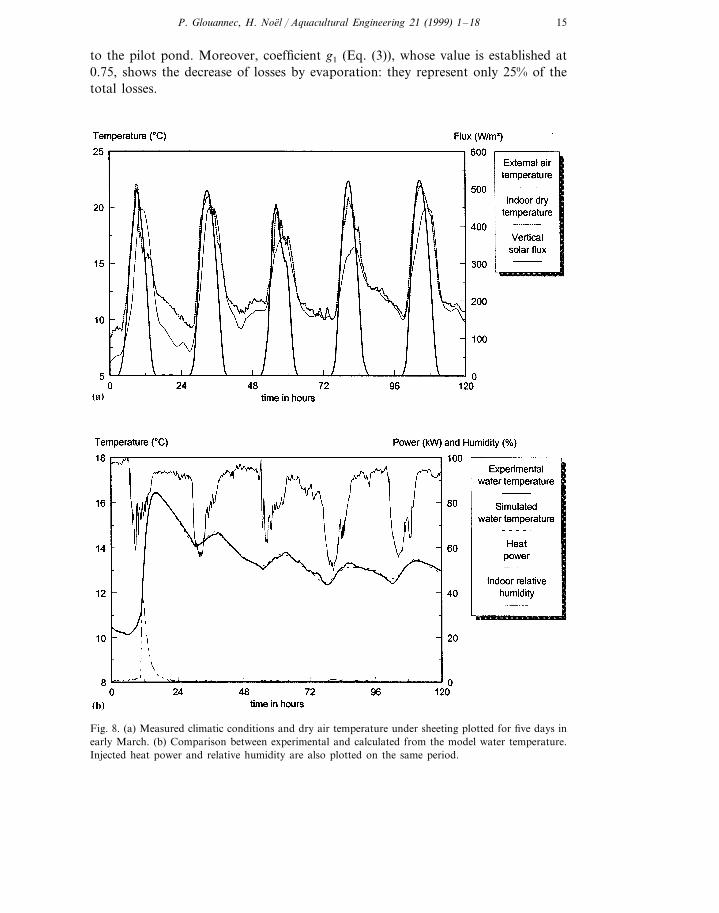
First, a sequence of measurements taken in winter is used to identify theparameters of the model. The chosen period was sunny, with mild air temperatures(Fig. 8a). The dry temperature measured under sheeting two metres above waterlevel, reaches relatively high levels. During the night, the relative humidity is near100% (Fig. 8b). A heating impulse was applied on the first day for a bettercharacterisation of the installation. An amplitude of 40 kW was measured for thepond under study.

In spite of dark sheeting, a first identifying testing was carried out by promptingthe model through three inputs: the external air temperature, the solar flux and thethermal power due to water supply. For the output variable, the average of the two


Fig. 7. (a) Diagram of the plant. (b) Setting up of the metrology (external dimensions: 5×4 m).

temperatures measured in the pond was used. In this particular plant, water is notinjected by injectors; yet, stratification remains limited due to an considerablerecycling flow rate of approximately 8 m3 h−1 for each pool. Taking insolation intoaccount leads to a very weak and even negative value for the solar surface.

Therefore, another test was made without introducing this prompting. In thiscase, the solar surface is obviously null and the parameters calculated have valuesthat are almost identical to the ones obtained previously (Fig. 8c). As can be noted,the calculation gives a high value for the global loss conductance Kg (58 W K−1)in spite of the protection covering. The fact that energy consumption was not takeninto account for the choice of the protection can explain this result. Furthermore,the ponds, which are made of concrete, are neither buried nor insulated. Thus, wehave greater losses by conductance and convection through the sidewalls, compared


to the pilot pond. Moreover, coefficient g1 (Eq. (3)), whose value is established at0.75, shows the decrease of losses by evaporation: they represent only 25% of thetotal losses.

Fig. 8. (a) Measured climatic conditions and dry air temperature under sheeting plotted for five days inearly March. (b) Comparison between experimental and calculated from the model water temperature.Injected heat power and relative humidity are also plotted on the same period.


Fig. 8. (Continued)

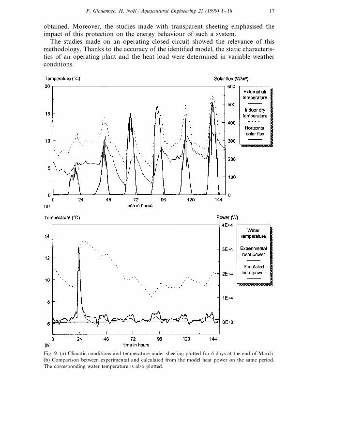
Fig. 8b shows the response to the identified model. This comparison with theexperimental curve may be considered satisfactory; nevertheless, the model wastested on another measuring sequence also made in winter, in order to confirm theanalysis. Fig. 9a shows the weather conditions and the evolution of the airtemperature measured under sheeting. The external air temperature remained lowduring this measuring sequence. A calculation of the heat load was made to test themodel. The study of Fig. 9b shows the significance of the procedure followed tocharacterise an operating plant. Indeed, the exploitation of this model on anothermeasuring sequence gave very satisfying results allowing to calculate the estimatedenergy consumption.

5. Conclusions

The studies presented aim at identifying the thermal characteristics of a closedcircuit aquacultural plant from in-situ readings. As noted previously, obtainingconsistent results implies carrying out recording sequences in variable weatherconditions while prompting correctly the installation with an intermittent heating.The experimental data obtained are processed by following a delayed time calcula-tion method that allows the development of a linear model representative of thetemperature response of the water volume.

Experiments were first carried out on a test pond during the winter period inorder to test and validate the methodology followed. Thus, even in the case of anopen pond with highly non-linear thermal exchanges, a quite pertinent model was


obtained. Moreover, the studies made with transparent sheeting emphasised theimpact of this protection on the energy behaviour of such a system.

The studies made on an operating closed circuit showed the relevance of thismethodology. Thanks to the accuracy of the identified model, the static characteris-tics of an operating plant and the heat load were determined in variable weatherconditions.

Fig. 9. (a) Climatic conditions and temperature under sheeting plotted for 6 days at the end of March.(b) Comparison between experimental and calculated from the model heat power on the same period.The corresponding water temperature is also plotted.


The studies presented in this article deal with the heating of the plant. Comple-mentary studies will be devoted to the cooling of the system. Furthermore, themodel established by identification can be used to elaborate an optimal commandalgorithm.

References

Cathcart, T.P., Wheaton, F.W., 1987. Modeling temperature distribution in freshwater ponds. Aquacul-tural Engineering 6, 237–257.

Cengel, Y.A., Ozizik, M.N., 1984. Solar radiation absorption in solar ponds. Solar Energy 33, 581–591.De Larminat, P., Thomas, Y., 1977. Automatique des systemes lineaires-2. Identification. Flammarion

Sciences ed. Isermann, R., 1989. Digital Control Systems, 1, Springer-Verlag ed. Kirk, J., 1988.Effect of scattering and absorption on solar pond efficiency. Solar Energy, 40, 107–116.

Klemetson, S.L., Rogers, G.L., 1985. Aquaculture pond temperature modeling. Aquacultural Engineer-ing 4, 191–208.

Marquardt, D.W., 1963. An algorithm for least-squares estimation of non linear parameters. J. Soc.Indust., Appl. Math. 11, 431–461.

Noel, H., Glouannec, P. and Velly, J.P. 1992. Modelisation du comportement thermique de bassinsdecouverts. Colloque SFT Systemes Thermiques Instationnaires, Sophia Antipolis.

Noel, H. 1993. Analyse experimentale et modelisation des echanges thermiques dans un bassin d’eaudouce-Application a l’aquaculture. ENSM Paris Thesis.

Noel, H., Glouannec, P., Velly, J.P., 1996. Mathematical Modelling and Experimental Validation of theThermal Behaviour of an Aquacultural Pond. Applied Energy 55, 47–64.

Perrin de Brichambaut, C., Vauge, C. 1982. Le gisement solaire. Lavoisier ed. Saulnier, J.B., AlexandreA., 1985. La modelisation thermique par la methode nodale, ses principes, ses succes et ses limites.Revue Generale de Thermique, 280, 363–371.

Semlyen, A., Dabuleanu, A., 1976. Fast and accurate switching transient calculations on transmissionlines with ground return using convolutions. IEEE trans. on circuits and systems 23, 56–58.

.

energy characterisation of an aquacultural installation in closed loop

Documents