chapter 12 closed-loop control system analysis
TRANSCRIPT
443
CHAPTER 12CLOSED-LOOP CONTROLSYSTEM ANALYSIS
Suhada JayasuriyaDepartment of Mechanical EngineeringTexas A&M UniversityCollege Station, Texas
1 INTRODUCTION 4441.1 Closed-Loop versus
Open-Loop Control 4451.2 Supervisory Control
Computers 4451.3 Hierarchical Control
Computers 4451.4 Direct Digital Control
(DDC) 4461.5 Hybrid Control 4461.6 Real Systems with Digital
Control 447
2 LAPLACE TRANSFORMS 4482.1 Single-Sided Laplace
Transform 4482.2 Transforming LTI Ordinary
Differential Equations 4502.3 Transfer Function 4512.4 Partial-Fraction Expansion
and Inverse Transform 4522.5 Inverse Transform by a
General Formula 456
3 BLOCK DIAGRAMS 4563.1 Block Diagram Reduction 4573.2 Transfer Functions of
Cascaded Elements 458
4 z-TRANSFORMS 4594.1 Single-Sided z-Transform 4614.2 Poles and Zeros in the
z-Plane 4614.3 z-Transforms of Some
Elementary Functions 4614.4 Some Important Properties
and Theorems of thez-Transform 462
4.5 Pulse Transfer Function 4634.6 Zero- and First-Order Hold 464
5 CLOSED-LOOPREPRESENTATION 468
5.1 Closed-Loop TransferFunction 468
5.2 Open-Loop TransferFunction 469
5.3 Characteristic Equation 4695.4 Standard Second-Order
Transfer Function 4715.5 Step Input Response of a
Standard Second-OrderSystem 472
5.6 Effects of an AdditionalZero and an Additional Pole 474
6 STABILITY 4756.1 Routh–Hurwitz Stability
Criterion 4756.2 Polar Plots 4816.3 Nyquist Stability Criterion 481
7 STEADY-STATEPERFORMANCE AND SYSTEMTYPE 4827.1 Step Input 4837.2 Ramp Input 4877.3 Parabolic Input 4887.4 Indices of Performance 4897.5 Integral-Square-Error (ISE)
Criterion 4897.6 Integral of Time-Multiplied
Absolute-Error (ITAE)Criterion 490
7.7 Comparison of VariousError Criteria 490
8 SIMULATION FOR CONTROLSYSTEM ANALYSIS 4908.1 Analog Computation 4928.2 Digital Computation 4988.3 Hybrid Computation 501
REFERENCES 501
BIBLIOGRAPHY 501
Reprinted from Instrumentation and Control, Wiley, New York, 1990, by permission of the publisher.
Mechanical Engineers’ Handbook: Instrumentation, Systems, Controls, and MEMS, Volume 2, Third Edition.Edited by Myer Kutz
Copyright 2006 by John Wiley & Sons, Inc.

444 Closed-Loop Control System Analysis
1 INTRODUCTION
The field of control has a rich heritage of intellectual depth and practical achievement. Fromthe water clock of Ctesibius in ancient Alexandria, where feedback control was used toregulate the flow of water, to the space exploration and the automated manufacturing plantsof today, control systems have played a very significant role in technological and scientificdevelopment. James Watt’s flyball governor (1769) was essential for the operation of thesteam engine, which was, in turn, a technology fueling the Industrial Revolution. The fun-damental study of feedback begins with James Clerk Maxwell’s analysis of system stabilityof steam engines with governors (1868). Giant strides in our understanding of feedback andits use in design resulted from the pioneering work of Black, Nyquist, and Bode at BellLabs in the l920s. Minorsky’s work on ship steering was of exceptional practical and theo-retical importance. Tremendous advances occurred during World War II in response to thepressing problems of that period. The technology developed during the war years led, overthe next 20 years, to practical applications in many fields.
Since the 1960s, there have been many challenges and spectacular achievements inspace. The guidance of the Apollo spacecraft on an optimized trajectory from the earth tothe moon and the soft landing on the moon depended heavily on control engineering. Today,the shuttle relies on automatic control in all phases of its flight. In aeronautics, the aircraftautopilot, the control of high-performance jet engines, and ascent /descent trajectory optim-ization to conserve fuel are typical examples of control applications. Currently, feedbackcontrol makes it possible to design aircraft that are aerodynamically unstable (such as theX-29) so as to achieve high performance. The National Aerospace Plane will rely on ad-vanced control algorithms to fly its demanding missions.
Control systems are providing dramatic new opportunities in the automotive industry.Feedback controls for engines permit federal emission levels to be met, while antiskid brak-ing control systems provide enhanced levels of passenger safety. In consumer products,control systems are often a critical factor in performance and thus economic success. Fromsimple thermostats that regulate temperature in buildings to the control of the optics forcompact disk systems, from garage door openers to the head servos for computer hard diskdrives, and from artificial hearts to remote manipulators, control applications have permeatedevery aspect of life in industrialized societies.
In process control, where systems may contain hundreds of control loops, adaptivecontrollers have been available commercially since 1983. Typically, even a small improve-ment in yield can be quite significant economically. Multivariable control algorithms are nowbeing implemented by several large companies. Moreover, improved control algorithms alsopermit inventories to be reduced, a particularly important consideration in processing dan-gerous material. In nuclear reactor control, improved control algorithms can have significantsafety and economic consequences. In power systems, coordinated computer control of alarge number of variables is becoming common. Over 30,000 computer control systems havebeen installed in the United States alone. Again, the economic impact of control is vast.
Accomplishments in the defense area are legion. The accomplishments range from theantiaircraft gunsights and the bombsights of World War II to the missile autopilots of todayand to the identification and estimation techniques used to track and designate multipletargets.
A large body of knowledge has come into existence as a result of these developmentsand continues to grow at a very rapid rate. A cross section of this body of knowledge iscollected in this chapter. It includes analysis tools and design methodologies based on clas-sical techniques. In presenting this material, some familiarity with general control systemdesign principles is assumed. As a result, detailed derivations have been kept to a minimumwith appropriate references.
1 Introduction 445
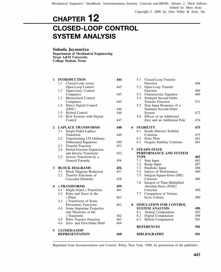
Figure 1 Closed-loop system configuration.
1.1 Closed-Loop versus Open-Loop Control
In a closed-loop control system the output is measured and used to alter the control inputsapplied to the plant under control. Figure 1 shows such a closed-loop system.
If output measurements are not utilized in determining the plant input, then the plant issaid to be under open-loop control. An open-loop control system is shown in Fig. 2.
An open-loop system is very sensitive to any plant parameter perturbations and anydisturbances that enter the plant. So an open-loop control system is effective only when theplant and disturbances are exactly known. In real applications, however, neither plants nordisturbances are exactly known a priori. In such situations open-loop control does not providesatisfactory performance. When the loop is closed as in Fig. 1 any plant perturbations ordisturbances can be sensed by measuring the outputs, thus allowing plant input to be alteredappropriately.
The main reason for closed-loop control is the need for systems to perform well in thepresence of uncertainties. It can reduce the sensitivity of the system to plant parametervariations and help reject or mitigate external disturbances. Among other attributes of closed-loop control is the ability to alter the overall dynamics to provide adequate stability andgood tracking characteristics. Consequently, a closed-loop system is more complex than anopen-loop system due to the required sensing of the output. Sensor noise, however, tends todegrade the performance of a feedback system, thus making it necessary to have accuratesensing. Therefore sensors are usually the most expensive devices in a feedback controlsystem.
1.2 Supervisory Control Computers1
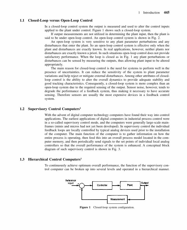
With the advent of digital computer technology computers have found their way into controlapplications. The earliest applications of digital computers in industrial process control werein a so-called supervisory control mode, and the computers were generally large-scale main-frames (minis and micros had not yet been developed). In supervisory control the individualfeedback loops are locally controlled by typical analog devices used prior to the installationof the computer. The main function of the computer is to gather information on how theentire process is operating, then feed this into an overall process model located in the com-puter memory, and then periodically send signals to the set points of individual local analogcontrollers so that the overall performance of the system is enhanced. A conceptual blockdiagram of such supervisory control is shown in Fig. 3.
1.3 Hierarchical Control Computers1
To continuously achieve optimum overall performance, the function of the supervisory con-trol computer can be broken up into several levels and operated in a hierarchical manner.
446 Closed-Loop Control System Analysis
Figure 2 Open-loop system configuration.
Figure 3 Supervisory control configuration.
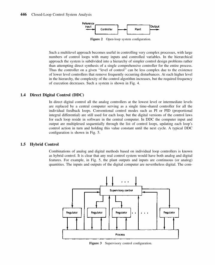
Such a multilevel approach becomes useful in controlling very complex processes, with largenumbers of control loops with many inputs and controlled variables. In the hierarchicalapproach the system is subdivided into a hierarchy of simpler control design problems ratherthan attempting direct synthesis of a single comprehensive controller for the entire process.Thus the controller on a given ‘‘level of control’’ can be less complex due to the existenceof lower level controllers that remove frequently occurring disturbances. At each higher levelin the hierarchy, the complexity of the control algorithm increases, but the required frequencyof execution decreases. Such a system is shown in Fig. 4.
1.4 Direct Digital Control (DDC)
In direct digital control all the analog controllers at the lowest level or intermediate levelsare replaced by a central computer serving as a single time-shared controller for all theindividual feedback loops. Conventional control modes such as PI or PID (proportionalintegral differential) are still used for each loop, but the digital versions of the control lawsfor each loop reside in software in the central computer. In DDC the computer input andoutput are multiplexed sequentially through the list of control loops, updating each loop’scontrol action in turn and holding this value constant until the next cycle. A typical DDCconfiguration is shown in Fig. 5.
1.5 Hybrid Control
Combinations of analog and digital methods based on individual loop controllers is knownas hybrid control. It is clear that any real control system would have both analog and digitalfeatures. For example, in Fig. 5, the plant outputs and inputs are continuous (or analog)quantities. The inputs and outputs of the digital computer are nevertheless digital. The com-
1 Introduction 447
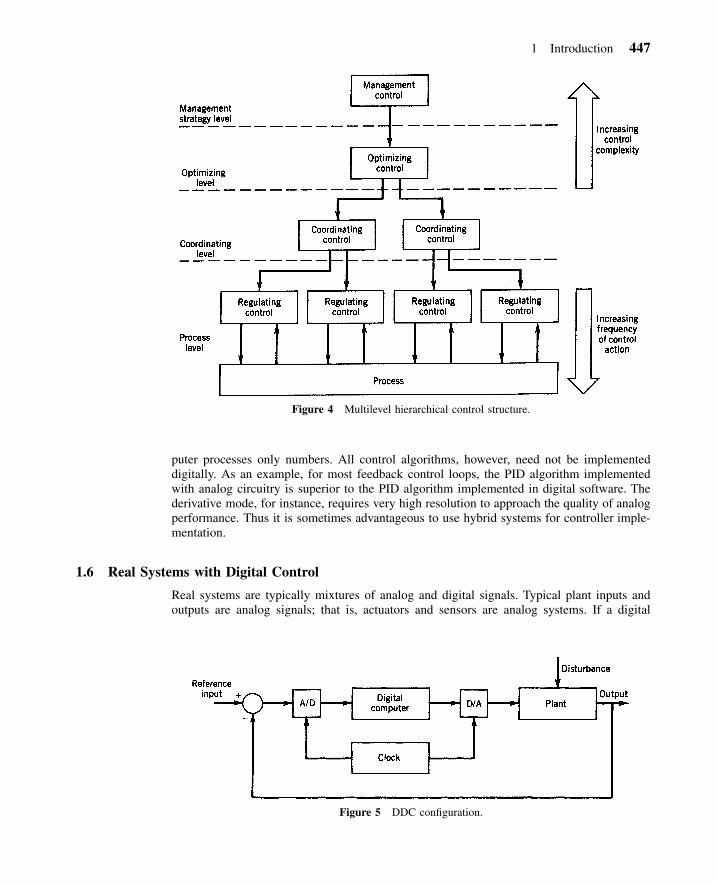
Figure 4 Multilevel hierarchical control structure.
Figure 5 DDC configuration.
puter processes only numbers. All control algorithms, however, need not be implementeddigitally. As an example, for most feedback control loops, the PID algorithm implementedwith analog circuitry is superior to the PID algorithm implemented in digital software. Thederivative mode, for instance, requires very high resolution to approach the quality of analogperformance. Thus it is sometimes advantageous to use hybrid systems for controller imple-mentation.
1.6 Real Systems with Digital Control
Real systems are typically mixtures of analog and digital signals. Typical plant inputs andoutputs are analog signals; that is, actuators and sensors are analog systems. If a digital
448 Closed-Loop Control System Analysis
computer is included in the control loop, then digitized quantities are needed for their proc-essing. These are usually accomplished by using analog-to-digital (A/D) converters. To usereal-world actuators, computations done as numbers need to be converted to analog signalsby employing digital-to-analog (D/A) converters. One of the main advantages of digitalcontrol is the ease with which an algorithm can be changed online by altering the softwarerather than hardware.
2 LAPLACE TRANSFORMS
Often in designing control systems, linear time-invariant (LTI) differential equation repre-sentations of physical systems to be controlled are sought. These are typically arrived at byappropriately linearizing the nonlinear equations about some operating point. The generalform of such an LTI ordinary differential equation representation is
n n�1d y(t) d y(t) dy(t)a � a � � � � � a � a y(t)n n�1 1 0n n�1dt dt dt
m m�1d d du(t)� b u(t) � b u(t) � � � � � b � b u(t) (1)m m�1 1 0m m�1dt dt dt
where y(t) � output of the systemu(t) � input to the system
t � timeaj, bj � physical parameters of the system
and n � m for physical systems.The ability to transform systems of the form given by Eq. (1) to algebraic equations
relating the input to the output is the primary reason for employing Laplace transform tech-niques.
2.1 Single-Sided Laplace Transform
The Laplace transform L [ƒ(t)] of the time function ƒ(t) defined as
0 t � 0ƒ(t) � �ƒ(t) t � 0
is given by
��st
L [ƒ(t)] � F(s) � � e ƒ(t) dt t � 0 (2)0
where s is a complex variable (� � j�). The integral of Eq. (2) cannot be evaluated in aclosed form for all ƒ(t), but when it can, it establishes a unique pair of functions, ƒ(t) in thetime domain and its companion F(s) in the s domain. It is conventional to use uppercaseletters for s functions and lowercase for t functions.
Example 1 Determine the Laplace transform of the unit step function us(t):
0 t � 0u (t) � �s 1 t � 0
2 Laplace Transforms 449
By definition
� 1�ts
L [u (t)] � U � � e 1 dt �s s0 s
Example 2 Determine the Laplace transform of ƒ(t):
0 t � 0ƒ(t) � � ��te t � 0
� 1�ts ��t
L [ƒ(t)] � F(s) � � e e dt �0 s � �
Example 3 Determine the Laplace transform of the function ƒ(t) given by
0 t � 0ƒ(t) � t 0 � t � T�T T � t
By definition
��tsF(s) � � e ƒ(t) dt
0
T ��ts �ts� � e t dt � � e T dt
0 T
�Ts1 e 1�Ts� � � (1 � e )2 2 2s s s
In transforming differential equations, entire equations need to be transformed. Severaltheorems useful in such transformations are given next without proof.
T1. Linearity Theorem
L [�ƒ(t) � �g(t)] � �L [ƒ(t)] � �L [g(t)] (3)
T2. Differentiation Theorem
dƒL � sF(s) � ƒ(0) (4)� �dt
2d ƒ dƒ2L � s F(s) � sƒ(0) � (0) (5)� �2dt dt
n n�1d ƒ dƒ dn n�1 n�2L � s F(s) � s ƒ(0) � s (0) � � � � � (0) (6)� �n n�1dt dt dt
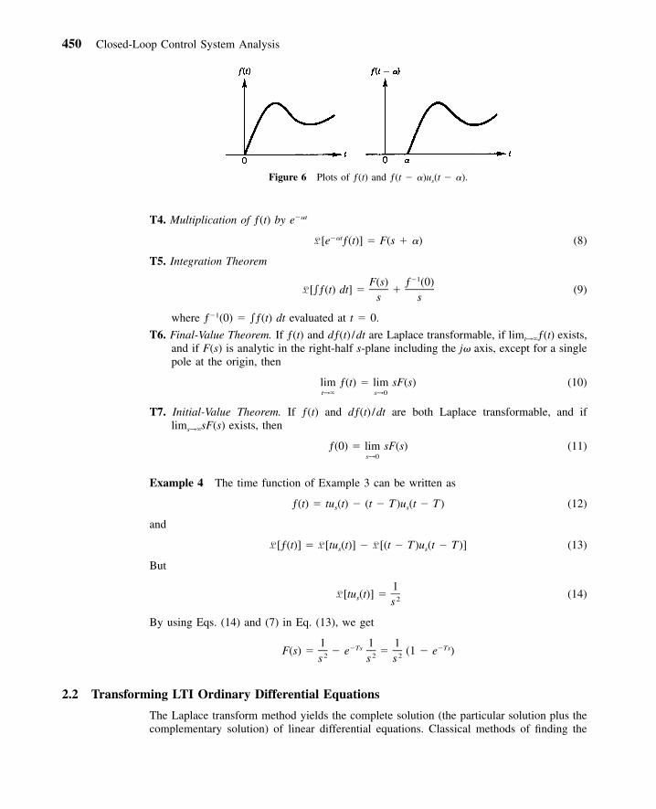
T3. Translated Function (Fig. 6)
��sL [ƒ(t � �)u (t � �)] � e F(s � �) (7)s
450 Closed-Loop Control System Analysis
Figure 6 Plots of ƒ(t) and ƒ(t � �)us(t � �).
T4. Multiplication of ƒ(t) by e��t
��tL [e ƒ(t)] � F(s � �) (8)
T5. Integration Theorem
�1F(s) ƒ (0)L [�ƒ(t) dt] � � (9)
s s
where ƒ�1(0) � �ƒ(t) dt evaluated at t � 0.
T6. Final-Value Theorem. If ƒ(t) and dƒ(t) /dt are Laplace transformable, if limt→�ƒ(t) exists,and if F(s) is analytic in the right-half s-plane including the j� axis, except for a singlepole at the origin, then
lim ƒ(t) � lim sF(s) (10)t→� s→0
T7. Initial-Value Theorem. If ƒ(t) and dƒ(t) /dt are both Laplace transformable, and iflims→�sF(s) exists, then
ƒ(0) � lim sF(s) (11)s→0
Example 4 The time function of Example 3 can be written as
ƒ(t) � tu (t) � (t � T )u (t � T ) (12)s s
and
L [ƒ(t)] � L [tu (t)] � L [(t � T )u (t � T )] (13)s s
But
1L [tu (t)] � (14)s 2s
By using Eqs. (14) and (7) in Eq. (13), we get
1 1 1�Ts �TsF(s) � � e � (1 � e )2 2 2s s s
2.2 Transforming LTI Ordinary Differential Equations
The Laplace transform method yields the complete solution (the particular solution plus thecomplementary solution) of linear differential equations. Classical methods of finding the
2 Laplace Transforms 451
complete solution of a differential equation require the evaluation of the integration constantsby use of the initial conditions. In the case of the Laplace transform method, initial conditionsare automatically included in the Laplace transform of the differential equation. If all initialconditions are zero, then the Laplace transform of the differential equation is obtained simplyby replacing d /dt with s, d 2 /dt 2 with s2, and so on.
Consider the differential equation
2d y5 � 3y � ƒ(t) (15)2dt
with � 1, y(0) � 0. By taking the Laplace transform of Eq. (15), we gety(0)
2d yL 5 � 3y � L [ƒ(t)]� �2dt
Now using Theorems T1 and T2 (page 449) yields
25[s Y(s) � sy(0) � y(0)] � 3Y(s) � F(s)
Thus
F(s) � 5Y(s) � (16)25s � 3
For a given ƒ(t), say ƒ(t) � us(t), the unit step function is given as
1F(s) � (17)
s
Substituting Eq. (17) in Eq. (16) gives
5s � 1Y(s) � 2s(5s � 3)
Then y(t) can be found by computing the inverse Laplace transform of Y(s). That is,
5s � 1�1 �1y(t) � L [Y(s)] � L � �2s(5s � 3)
This will be discussed in Section 2.4.
2.3 Transfer Function
The transfer function of a LTI system is defined to be the ratio of the Laplace transform ofthe output to the Laplace transform of the input under the assumption that all initial con-ditions are zero.
For the system described by the LTI differential equation (1),
L [output] L [y(t)] Y(s)� �
L [input] L [u(t)] U(s)
m m�1b s � b s � � � � � b s � bm m�1 1 0� (18)n n�1a s � a s � � � � � a s � an n�1 1 0
It should be noted that the transfer function depends only on the system parameterscharacterized by ai’s and bi’s in Eq. (18). The highest power of s in the denominator of the
452 Closed-Loop Control System Analysis
transfer function defines the order n of the system. The order n of a system is typicallygreater than or equal to the order of the numerator polynomial m.
Equation (18) can be further written in the form
mb (s � z )�m j�1 iY(s)� G(s) � (19)nU(s) a (s � p )�n j�1 j
The values of s making Eq. (19) equal to zero are called the system zeros, and thevalues of s making Eq. (19) go to � are called poles of the system. Hence s � �zi, i � 1,. . . , m, are the system zeros and s � �pj, j � 1, . . . , n, are the system poles.
2.4 Partial-Fraction Expansion and Inverse Transform
The mathematical process of passing from the complex variable expression F(s) to the time-domain expression ƒ(t) is called an inverse transformation. The notation for the inverseLaplace transformation is L
�1, so that
�1L [F(s)] � ƒ(t)
Example 5 The inverse Laplace transform of 1/s is the unit step function:
1L [u (t)] �s s
Hence
1�1
L � u (t)� ss
Time functions for which Laplace transforms are found in a closed form can be readilyinverse Laplace transformed by writing them in pairs. Such pairs are listed in Table 1. Whentransform pairs are not found in tables, other methods have to be used to find the inverseLaplace transform. One such method is the partial-fraction expansion of a given Laplacetransform.
If F(s), the Laplace transform of ƒ(t), is broken up into components
F(s) � F (s) � F (s) � � � � � F (s)1 2 n
and if the inverse Laplace transforms of F1(s), F2(s), . . . , Fn(s) are readily available, then
�1 �1 �1 �1L [F(s)] � L [F (s)] � L [F (s)] � � � � � L [F (s)]1 2 n
� ƒ (t) � ƒ (t) � � � � � ƒ (t) (20)1 2 n
where ƒ1(t), ƒ2(t), . . . , ƒn(t) are the inverse Laplace transforms of F1(s), F2(s), . . . , Fn(s),respectively.
For problems in control systems, F(s) is frequently in the form
B(s)F(s) �
A(s)
where A(s) and B(s) are polynomials in s and the degree of B(s) is equal to or higher thanthat of A(s).
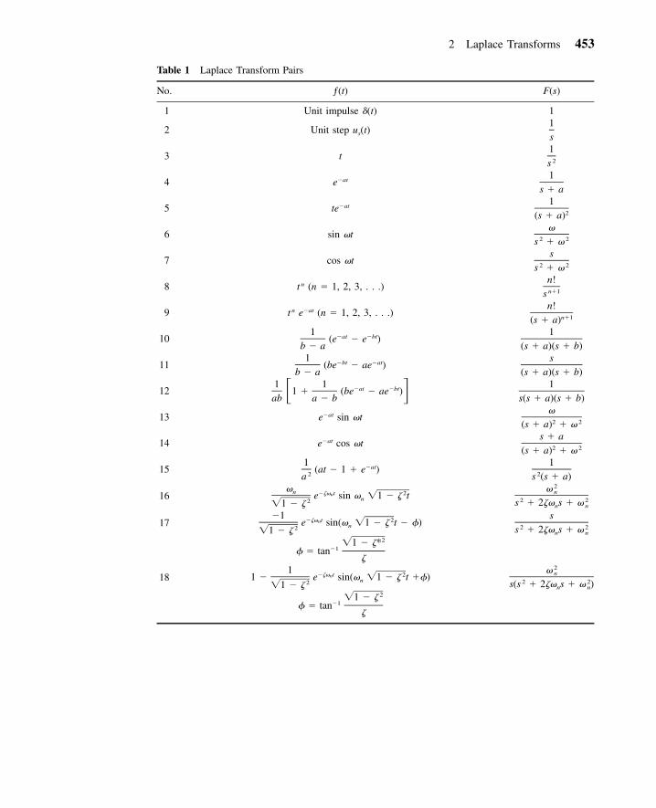
2 Laplace Transforms 453
Table 1 Laplace Transform Pairs
No. ƒ(t) F(s)
1 Unit impulse �(t) 1
2 Unit step us(t)1s
3 t1
2s
4 e�at1
s � a
5 te�at1
2(s � a)
6 sin �t�
2 2s � �
7 cos �ts
2 2s � �
8 t n (n � 1, 2, 3, . . .)n!n�1s
9 t n e�at (n � 1, 2, 3, . . .)n!
n�1(s � a)
101
�at �bt(e � e )b � a
1(s � a)(s � b)
111
�bt �at(be � ae )b � a
s(s � a)(s � b)
121 1
�at �bt1 � (be � ae )� �ab a � b1
s(s � a)(s � b)
13 e�at sin �t�
2 2(s � a) � �
14 e�at cos �ts � a
2 2(s � a) � �
151
�at(at � 1 � e )2a
12s (s � a)
16�n ��� t 2ne sin � 1 � � tn21 � �
2� n
2 2s � 2�� s � �n n
17�1
��� t 2ne sin(� 1 � � t � )n21 � �
s2 2s � 2�� s � �n n
21 � �*�1 � tan
�
181
��� t 2n1 � e sin(� 1 � � t �)n21 � �
2� n
2 2s(s � 2�� s � � )n n21 � �
�1 � tan�
454 Closed-Loop Control System Analysis
If F(s) is written as in Eq. (19) and if the poles of F(s) are distinct, then F(s) can alwaysbe expressed in terms of simple partial fractions as follows:
B(s) � � �1 2 nF(s) � � � � � � � � (21)A(s) s � p s � p s � p1 2 n
where the �j’s are constant. Here �j is called the residue at the pole s � �pj. The value of�j is found by multiplying both sides of Eq. (21) by s � pj and setting s � �pj, giving
B(s)� � (s � p ) (22)� �j j A(s) s�pj
Noting that
1�1 �p tjL � e� �s � pj
the inverse Laplace transform of Eq. (21) can be written as
n�1 �p tjƒ(t) � L [F(s)] � � e (23)� j
j�1
Example 6 Find the inverse Laplace transform of
s � 1F(s) �
(s � 2)(s � 3)
The partial-fraction expansion of F(s) is
s � 1 � �1 2F(s) � � �(s � 2)(s � 3) s � 2 s � 3
where �1 and �2 are found by using Eq. (22) as follows:
s � 1� � (s � 2) � �1� �1 (s � 2)(s � 3) s��2
s � 1� � (s � 3) � 2� �2 (s � 2)(s � 3) s��3
Thus
�1 2�1 �1ƒ(t) � L � L� � � �s � 2 s � 3
�2t �3t� �e � 2e t � 0
For partial-fraction expansion when F(s) involves multiple poles, consider
mK (s � z )�i�1 i B(s)F(s) � �nr A(s)(s � p ) (s � p )�1 j�r�1 j
where the pole at s � �p1 has multiplicity r. The partial-fraction expansion of F(s) maythen be written as
2 Laplace Transforms 455
B(s) � � �1 2 rF(s) � � � � � � � �2 rA(s) s � p (s � p ) (s � p )1 1 1
n �j� (24)�
s � pj�r�1 j
The �j’s can be evaluated as before using Eq. (22). The �i’s are given by
B(s) r� � (s � p )� �r 1A(s) s��p1
d B(s) r� � (s � p )� � ��r�1 1ds A(s) s��p1
�
j1 d B(s) r� � (s � p )� � ��r�j 1jj! ds A(s) s��p1
�
r�11 d B(s) r� � (s � p )� � ��1 1r�1(r � 1)! ds A(s) s��p1
The inverse Laplace transform of Eq. (24) can then be obtained as follows:
� �r r�1r�1 r�2 �p t1ƒ(t) � t � t � � � � � � t � � e� �2 1(r � 1)! (r � 2)!
n�p t1� � e t � 0 (25)� j
j�r�1
Example 7 Find the inverse Laplace transform of the function
2s � 2s � 3F(s) � 3(s � 1)
Expanding F(s) into partial fractions, we obtain
B(s) � � �1 2 3F(s) � � � �2 3A(s) s � 1 (s � 1) (s � 1)
where �1, �2, and �3 are determined as already shown:
B(s) 3� � (s � 1) � 2� �3 A(s) s��1
similarly �2 � 0 and �1 � 1. Thus we get
1 2�1 �1ƒ(t) � L � L� � � �3s � 1 (s � 1)
�t 2 �t� e � t e t � 0
456 Closed-Loop Control System Analysis
Figure 7 Path of integration.
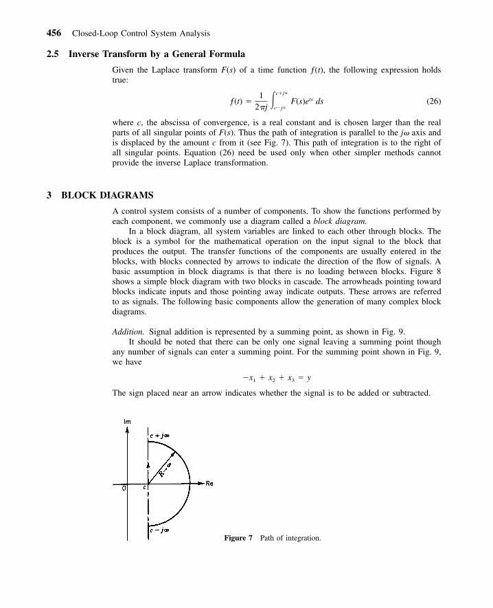
2.5 Inverse Transform by a General Formula
Given the Laplace transform F(s) of a time function ƒ(t), the following expression holdstrue:
c�j�1 tsƒ(t) � � F(s)e ds (26)c�j�2j
where c, the abscissa of convergence, is a real constant and is chosen larger than the realparts of all singular points of F(s). Thus the path of integration is parallel to the j� axis andis displaced by the amount c from it (see Fig. 7). This path of integration is to the right ofall singular points. Equation (26) need be used only when other simpler methods cannotprovide the inverse Laplace transformation.
3 BLOCK DIAGRAMS
A control system consists of a number of components. To show the functions performed byeach component, we commonly use a diagram called a block diagram.
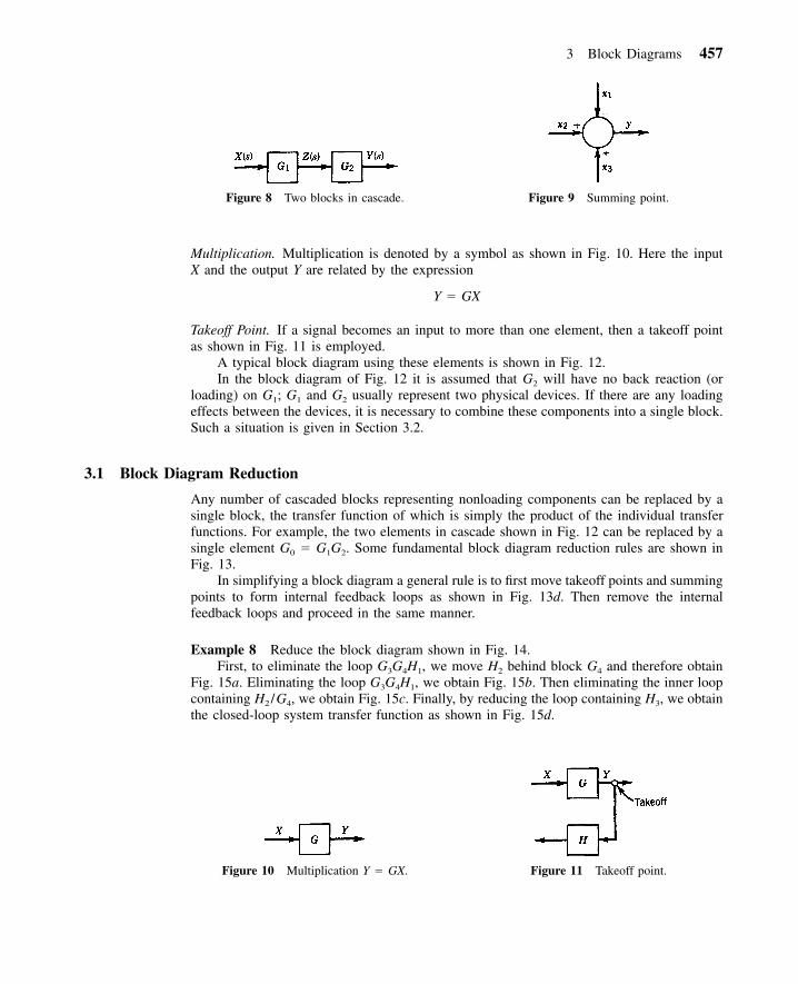
In a block diagram, all system variables are linked to each other through blocks. Theblock is a symbol for the mathematical operation on the input signal to the block thatproduces the output. The transfer functions of the components are usually entered in theblocks, with blocks connected by arrows to indicate the direction of the flow of signals. Abasic assumption in block diagrams is that there is no loading between blocks. Figure 8shows a simple block diagram with two blocks in cascade. The arrowheads pointing towardblocks indicate inputs and those pointing away indicate outputs. These arrows are referredto as signals. The following basic components allow the generation of many complex blockdiagrams.
Addition. Signal addition is represented by a summing point, as shown in Fig. 9.It should be noted that there can be only one signal leaving a summing point though
any number of signals can enter a summing point. For the summing point shown in Fig. 9,we have
�x � x � x � y1 2 3
The sign placed near an arrow indicates whether the signal is to be added or subtracted.
3 Block Diagrams 457
Figure 8 Two blocks in cascade. Figure 9 Summing point.
Figure 10 Multiplication Y � GX. Figure 11 Takeoff point.
Multiplication. Multiplication is denoted by a symbol as shown in Fig. 10. Here the inputX and the output Y are related by the expression
Y � GX
Takeoff Point. If a signal becomes an input to more than one element, then a takeoff pointas shown in Fig. 11 is employed.
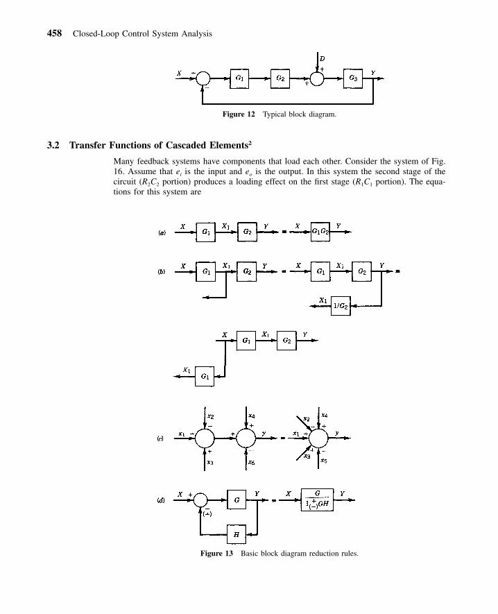
A typical block diagram using these elements is shown in Fig. 12.In the block diagram of Fig. 12 it is assumed that G2 will have no back reaction (or
loading) on G1; G1 and G2 usually represent two physical devices. If there are any loadingeffects between the devices, it is necessary to combine these components into a single block.Such a situation is given in Section 3.2.
3.1 Block Diagram Reduction
Any number of cascaded blocks representing nonloading components can be replaced by asingle block, the transfer function of which is simply the product of the individual transferfunctions. For example, the two elements in cascade shown in Fig. 12 can be replaced by asingle element G0 � G1G2. Some fundamental block diagram reduction rules are shown inFig. 13.
In simplifying a block diagram a general rule is to first move takeoff points and summingpoints to form internal feedback loops as shown in Fig. 13d. Then remove the internalfeedback loops and proceed in the same manner.
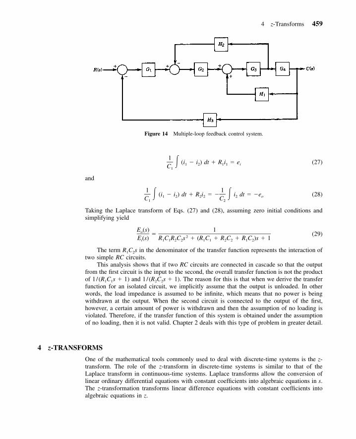
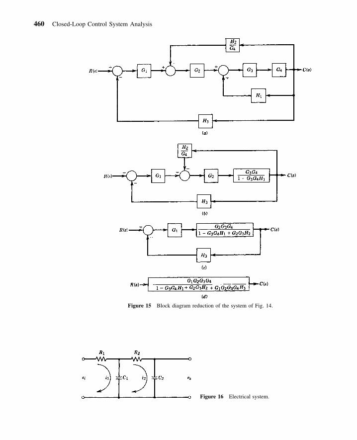
Example 8 Reduce the block diagram shown in Fig. 14.First, to eliminate the loop G3G4H1, we move H2 behind block G4 and therefore obtain
Fig. 15a. Eliminating the loop G3G4H1, we obtain Fig. 15b. Then eliminating the inner loopcontaining H2 /G4, we obtain Fig. 15c. Finally, by reducing the loop containing H3, we obtainthe closed-loop system transfer function as shown in Fig. 15d.
458 Closed-Loop Control System Analysis
Figure 12 Typical block diagram.
Figure 13 Basic block diagram reduction rules.
3.2 Transfer Functions of Cascaded Elements2
Many feedback systems have components that load each other. Consider the system of Fig.16. Assume that ei is the input and eo is the output. In this system the second stage of thecircuit (R2C2 portion) produces a loading effect on the first stage (R1C1 portion). The equa-tions for this system are
4 z-Transforms 459
Figure 14 Multiple-loop feedback control system.
1 � (i � i ) dt � R i � e (27)1 2 1 1 iC1
and
1 1� (i � i ) dt � R i � � � i dt � �e (28)1 2 2 2 2 oC C1 2
Taking the Laplace transform of Eqs. (27) and (28), assuming zero initial conditions andsimplifying yield
E (s) 1o � (29)2E (s) R C R C s � (R C � R C � R C )s � 1i 1 1 2 2 1 1 2 2 1 2
The term R1C2s in the denominator of the transfer function represents the interaction oftwo simple RC circuits.
This analysis shows that if two RC circuits are connected in cascade so that the outputfrom the first circuit is the input to the second, the overall transfer function is not the productof 1/ (R1C1s � 1) and 1/(R2C2s � 1). The reason for this is that when we derive the transferfunction for an isolated circuit, we implicitly assume that the output is unloaded. In otherwords, the load impedance is assumed to be infinite, which means that no power is beingwithdrawn at the output. When the second circuit is connected to the output of the first,however, a certain amount of power is withdrawn and then the assumption of no loading isviolated. Therefore, if the transfer function of this system is obtained under the assumptionof no loading, then it is not valid. Chapter 2 deals with this type of problem in greater detail.
4 z-TRANSFORMS
One of the mathematical tools commonly used to deal with discrete-time systems is the z-transform. The role of the z-transform in discrete-time systems is similar to that of theLaplace transform in continuous-time systems. Laplace transforms allow the conversion oflinear ordinary differential equations with constant coefficients into algebraic equations in s.The z-transformation transforms linear difference equations with constant coefficients intoalgebraic equations in z.
460 Closed-Loop Control System Analysis
Figure 15 Block diagram reduction of the system of Fig. 14.
Figure 16 Electrical system.

4 z-Transforms 461
4.1 Single-Sided z-Transform
If a signal has discrete values ƒ0, ƒ1, . . . , ƒk, . . . , we define the z-transform of the signalas the function
F(z) � Z {ƒ(k)}
��k� ƒ(k)z r � �z� � R (30)� 0 0
k�0
and is assumed that one can find a range of values of the magnitude of the complex variablez for which the series of Eq. (30) converges. This z-transform is referred to as the one-sidedz-transform. The symbol Z denotes ‘‘the z-transform of.’’ In the one-sided z-transform it isassumed ƒ(k) � 0 for k � 0, which in the continuous-time case corresponds to ƒ(t) � 0 fort � 0.
Expansion of the right-hand side of Eq. (30) gives�1 �2 �kF(z) � ƒ(0) � ƒ(1)z � ƒ(2)z � � � � � ƒ(k)z � � � � (31)
The last equation implies that the z-transform of any continuous-time function ƒ(t) maybe written in the series form by inspection. The z�k in this series indicates the instant in timeat which the amplitude ƒ(k) occurs. Conversely, if F(z) is given in the series form of Eq.(31), the inverse z-transform can be obtained by inspection as a sequence of the functionƒ(k) that corresponds to the values of ƒ(t) at the respective instants of time. If the signal issampled at a fixed sampling period T, then the sampled version of the signal ƒ(t) given byƒ(0), ƒ(1), . . . , ƒ(k) correspond to the signal values at the instants 0, T, 2T, . . . , kT.
4.2 Poles and Zeros in the z-Plane
If the z-transform of a function takes the formm m�1b z � b z � � � � � b0 1 mF(z) � (32)n n�1z � a z � � � � � a1 n
or
b (z � z )(z � z ) � � � (z � z )0 1 2 mF(z) �(z � p )(z � p ) � � � (z � p )1 2 n
then pi’s are the poles of F(z) and zi’s are the zeros of F(z).In control studies, F(z) is frequently expressed as a ratio of polynomials in z�1 as
follows:�(n�m) �(n�m�1) �nb z � b z � � � � � b z0 1 mF(z) � (33)
�1 �2 �n1 � a z � a z � � � � � a z1 2 n
where z�1 is interpreted as the unit delay operator.
4.3 z-Transforms of Some Elementary Functions
Unit Step FunctionConsider the unit step function
1 t � 0u (t) � �s 0 t � 0
whose discrete representation is
462 Closed-Loop Control System Analysis
1 k � 0u (k) � �s 0 k � 0
From Eq. (30)
� ��k �k �1 �2
Z {u (k)} � 1 �z � z � 1 � z � z � � � �� �sk�0 k�0
1 z� � (34)
�11 � z z � 1
Note that the series converges for �z� � 1. In finding the z-transform, the variable z acts asa dummy operator. It is not necessary to specify the region of z over which Z {us(k)} isconvergent. The z-transform of a function obtained in this manner is valid throughout the z-plane except at the poles of the transformed function. The us(k) is usually referred to as theunit step sequence.
Exponential FunctionLet
�ate t � 0ƒ(t) � �0 t � 0
The sampled form of the function with sampling period T is
�akTƒ(kT ) � e k � 0, 1, 2, . . .
By definition
F(z) � Z {ƒ(k)}
��k� ƒ(k)z�
k�0
��akt �k� e z�
k�0
�at �1 �2at �2� 1 � e z � e z � � � �
1�
�at �11 � e z
z�
�atz � e
4.4 Some Important Properties and Theorems of the z-Transform
In this section some useful properties and theorems are stated without proof. It is assumedthat the time function ƒ(t) is z-transformable and that ƒ(t) is zero for t � 0.
P1. If
F(z) � Z {ƒ(k)}
then

4 z-Transforms 463
Z {aƒ(k)} � aF(z) (35)
P2. If ƒ1(k) and g1(k) are z-transformable and � and � are scalars, then ƒ(k) � �ƒ1(k) ��g1(k) has the z-transform
F(z) � �F (z) � �G (z) (36)1 1
where F1(z) and G1(z) are the z-transforms of ƒ1(k) and g1(k), respectively.
P3. If
F(z) � Z {ƒ(k)}
then
zkZ {a ƒ(k)} � F (37)� a
T1. Shifting Theorem. If ƒ(t) � 0 for t � 0 and ƒ(t) has the z-transform F(z), then
�nZ {ƒ(t � nT )} � z F(z)
and
n�1n �k
Z {ƒ(t � nT )} � z F(z) � ƒ(kT )z (38)�� �k�0
T2. Complex Translation Theorem. If
F(z) � Z {ƒ(t)}
then
�at atZ {e ƒ(t)} � F(ze ) (39)
T3. Initial-Value Theorem. If F(z) � Z {ƒ(t)} and if limz→� F(z) exists, then the initial valueƒ(0) of ƒ(t) or ƒ(k) is given by
ƒ(0) � lim F(z) (40)z→�
T4. Final-Value Theorem. Suppose that ƒ(k), where ƒ(k) � 0 for k � 0, has the z-transformF(z) and that all the poles of F(z) lie inside the unit circle, with the possible exceptionof a simple pole at z � 1. Then the final value of ƒ(k) is given by
�1lim ƒ(k) � lim [(1 � z )F(z)] (41)k→� z→1
4.5 Pulse Transfer Function
Consider the LTI discrete-time system characterized by the following linear difference equa-tion:
y(k) � a y(k � 1) � � � � � a y(k � n) � b u(k) � b u(k � 1) � � � � � b u(k � m) (42)1 n 0 1 m
where u(k) and y(k) are the system’s input and output, respectively, at the kth sampling orat the real time kT; T is the sampling period. To convert the difference equation (42) to analgebraic equation, take the z-transform of both sides of Eq. (42) by definition:
464 Closed-Loop Control System Analysis
Z {y(k)} � Y(z) (43a)
Z {u(k)} � U(z) (43b)
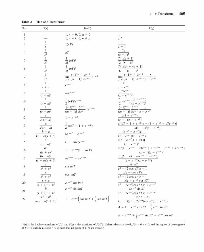
By referring to Table 2, the z-transform of Eq. (42) becomes
�1 �n �1 �mY(z) � a z (Y(z) � � � � � a z y(z) � b U(z) � b z U(z) � � � � � b z U(z)1 n 0 1 m
or
�1 �1 �1 �m[1 � a z � � � � � a z ]Y(z) � [b � b z � � � � � b z ]U(z)1 n 0 1 m
which can be written as
�1 �mY(z) b � b z � � � � � b z0 1 m� (44)�1 �nU(z) 1 � a z � � � � � a z1 n
Consider the response of the linear discrete-time system given by Eq. (44), initially at restwhen the input u(t) is the delta ‘‘function’’ �(kT ),
1 k � 0�(kT ) � �0 k 0
since
��k
Z {�(kT )} � �(kT )z � 1�k�0
U(z) � Z {�(kT )} � 1
and
�1 �mb � b z � � � � � b z0 1 mY(z) � � G(z) (45)�1 �n1 � a z � � � � � a z1 n
Thus G(z) is the response of the system to the delta input (or unit impulse) and plays thesame role as the transfer function in linear continuous-time systems. The function G(z) iscalled the pulse transfer function.
4.6 Zero- and First-Order Hold
Discrete-time control systems may operate partly in discrete time and partly in continuoustime. Replacing a continuous-time controller with a digital controller necessitates the con-version of numbers to continuous-time signals to be used as true actuating signals. Theprocess by which a discrete-time sequence is converted to a continuous-time signal is calleddata hold.
In a conventional sampler, a switch closes to admit an input signal every sample periodT. In practice, the sampling duration is very small compared with the most significant timeconstant of the plant. Suppose the discrete-time sequence is ƒ(kT ); then the function of thedata hold is to specify the values for a continuous equivalent h(t) where kT � t � (k � 1)T.In general, the signal h(t) during the time interval kT � t � (k � 1)T may be approximatedby a polynomial in � as follows:
n n�1h(kT � �) � a � � a � � � � � � a � � a (46)n n�1 1 0
where 0 � � � T. Since the value of the continuous equivalent must match at the samplinginstants, one requires
4 z-Transforms 465
Table 2 Table of z-Transforms a
No. F(s) ƒ(nT ) F(z)
1 — 1, n � 0; 0, n 0 12 — 1, n � k; 0, n k z�k
31s
1(nT )z
z � 1
41
2snT
Tz2(z � 1)
51
3s1
2(nT )2!
2T z(z � 1)32 (z � 1)
61
4s1
3(nT )3!
3 2T z(z � 4z � 1)46 (z � 1)
71ms
m�1 m�1(�1) ��unTlim e
m�1(m � 1)! �aa→0
m�1 m�1(�1) � zlim
m�1 �aT(m � 1)! �a z � ea→0
81
s � ae�anT
z�aTz � e
91
2(s � a)nTe�anT
�aTTze�aT 2(z � e )
101
3(s � a)1
2 �anT(nT ) e2
2 �aTT z(z � e )�aT(e )
�aT 32 (z � e )
111
m(s � a)
m�1 m�1(�1) ��anT(e )
m�1(m � 1)! �a
m�1 m�1(�1) � zm�1 �aT(m � 1)! �a z � e
12a
s(s � a)1 � e�anT
�aTz(1 � e )�aT(z � 1)(z � e )
13a
2s (s � a)1
�anT(anT � 1 � e )a
�aT �aT �aTz[(aT � 1 � e )z � (1 � e � aTe )]2 �aTa(z � 1) (z � e )
14b � a
(s � a)(s � b)(e�anT � e�bnT )
�aT �bT(e � e )z�aT �bT(x � e )(z � e )
15s
2(s � a)(1 � anT )e�anT
�aTz[z � e (1 � aT )]�aT 2(z � e )
162a
2s(s � a)1 � e�anT(1 � anT )
�aT �aT �2aT �aT �aTz[z(1 � e � aTe ) � e � e � aTe ]�aT 2(z � 1)(z � e )
17(b � a)s
(s � a)(s � b)be�bnT � ae�anT
�aT �bTz[z(b � a) � (be � ae )]�aT �bT(z � e )(z � e )
18a
2 2s � asin anT
z sin aT2z � (2 cos aT )z � 1
19s
2 2s � acos anT
z(z � cos aT )2z � (2 cos aT )z � 1
20s � a
2 2(s � a) � be�anT cos bnT
�aTz(z � e cos bT )2 �aT �2eTz � 2e (cos bT )z � e
21b
2 2(s � a) � be�anT sin bnT �aTze sin bT
2 �aT �2aTz � 2e (cos bT )z � e
222 2a � b
2 2s((s � a) � b )a
�anT1 � e cos bnT � sin bnT� bz(Az � B)
2 �aT �2aT(z � 1)(z � 2e (cos bT )z � e )a
�aT �aTA � 1 � e cos bT � e sin bTb
a�2aT �aT �aTB � e � e sin bT � e cos bT
b
aF(s) is the Laplace transform of ƒ(t) and F(z) is the transform of ƒ(nT ). Unless otherwise noted, ƒ(t) � 0, t � 0, and the region of convergence
of F(z) is outside a circle r � �z� such that all poles of F(z) are inside r.
466 Closed-Loop Control System Analysis
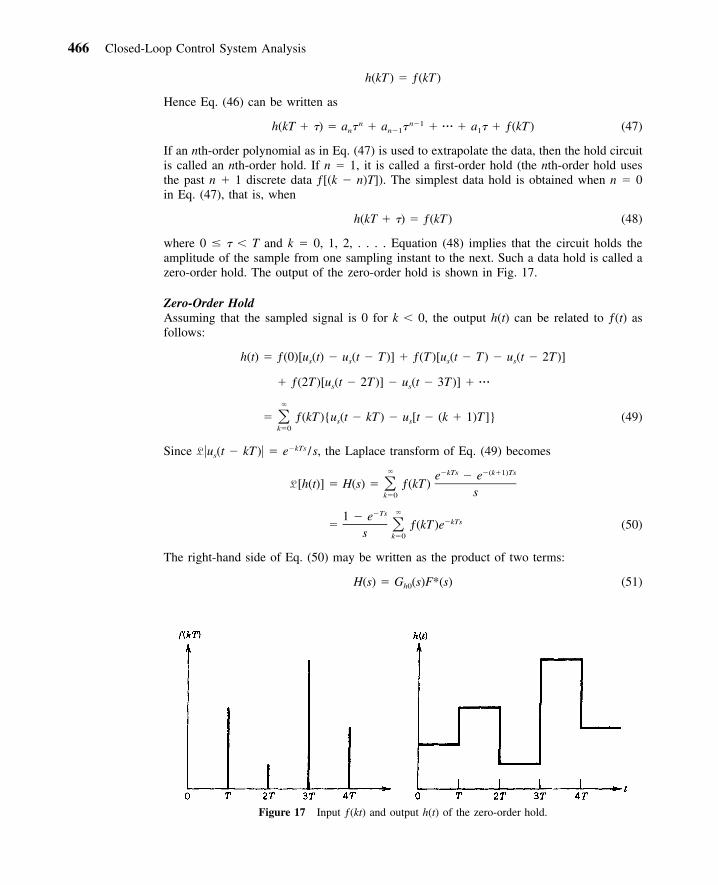
Figure 17 Input ƒ(kt) and output h(t) of the zero-order hold.
h(kT ) � ƒ(kT )
Hence Eq. (46) can be written as
n n�1h(kT � �) � a � � a � � � � � � a � � ƒ(kT ) (47)n n�1 1
If an nth-order polynomial as in Eq. (47) is used to extrapolate the data, then the hold circuitis called an nth-order hold. If n � 1, it is called a first-order hold (the nth-order hold usesthe past n � 1 discrete data ƒ[(k � n)T]). The simplest data hold is obtained when n � 0in Eq. (47), that is, when
h(kT � �) � ƒ(kT ) (48)
where 0 � � � T and k � 0, 1, 2, . . . . Equation (48) implies that the circuit holds theamplitude of the sample from one sampling instant to the next. Such a data hold is called azero-order hold. The output of the zero-order hold is shown in Fig. 17.
Zero-Order HoldAssuming that the sampled signal is 0 for k � 0, the output h(t) can be related to ƒ(t) asfollows:
h(t) � ƒ(0)[u (t) � u (t � T )] � ƒ(T )[u (t � T ) � u (t � 2T )]s s s s
� ƒ(2T )[u (t � 2T )] � u (t � 3T )] � � � �s s
�
� ƒ(kT ){u (t � kT ) � u [t � (k � 1)T ]} (49)� s sk�0
Since L �us(t � kT )� � e�kTs /s, the Laplace transform of Eq. (49) becomes
� �kTs �(k�1)Tse � eL [h(t)] � H(s) � ƒ(kT )�
sk�0
��Ts1 � e�kTs� ƒ(kT )e (50)�
s k�0
The right-hand side of Eq. (50) may be written as the product of two terms:
H(s) � G (s)F*(s) (51)h0
4 z-Transforms 467
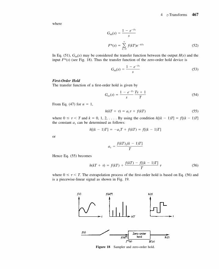
Figure 18 Sampler and zero-order hold.
where
�Ts1 � eG (s) �h0 s
��kTsF*(s) � ƒ(kT )e (52)�
k�0
In Eq. (51), Gh0(s) may be considered the transfer function between the output H(s) and theinput F*(s) (see Fig. 18). Thus the transfer function of the zero-order hold device is
�Ts1 � eG (s) � (53)h0 s
First-Order HoldThe transfer function of a first-order hold is given by
�Ts1 � e Ts � 1G (s) � (54)h1 s T
From Eq. (47) for n � 1,
h(kT � �) � a � � ƒ(kT ) (55)1
where 0 � � � T and k � 0, 1, 2, . . . . By using the condition h[(k � 1)T] � ƒ[(k � 1)T]the constant a1 can be determined as follows:
h[(k � 1)T ] � �a T � ƒ(kT ) � ƒ[(k � 1)T ]1
or
ƒ(kT ) (k � 1)T ]ƒa �1 T
Hence Eq. (55) becomes
ƒ(kT ) � ƒ[(k � 1)T ]h(kT � �) � ƒ(kT ) � � (56)
T
where 0 � � � T. The extrapolation process of the first-order hold is based on Eq. (56) andis a piecewise-linear signal as shown in Fig. 19.
468 Closed-Loop Control System Analysis
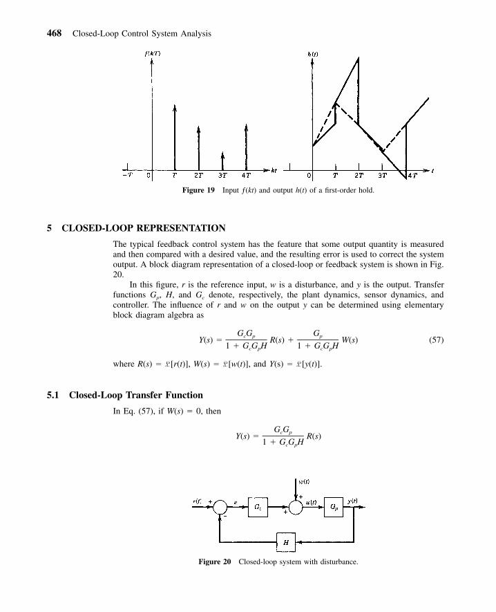
Figure 19 Input ƒ(kt) and output h(t) of a first-order hold.
Figure 20 Closed-loop system with disturbance.
5 CLOSED-LOOP REPRESENTATION
The typical feedback control system has the feature that some output quantity is measuredand then compared with a desired value, and the resulting error is used to correct the systemoutput. A block diagram representation of a closed-loop or feedback system is shown in Fig.20.
In this figure, r is the reference input, w is a disturbance, and y is the output. Transferfunctions Gp, H, and Gc denote, respectively, the plant dynamics, sensor dynamics, andcontroller. The influence of r and w on the output y can be determined using elementaryblock diagram algebra as
G G Gc p pY(s) � R(s) � W(s) (57)
1 � G G H 1 � G G Hc p c p
where R(s) � L [r(t)], W(s) � L [w(t)], and Y(s) � L [y(t)].
5.1 Closed-Loop Transfer Function
In Eq. (57), if W(s) � 0, then
G Gc pY(s) � R(s)
1 � G G Hc p
5 Closed-Loop Representation 469
Figure 21 Closed-loop system.
or alternatively a transfer function called the closed-loop transfer function between the ref-erence input and the output is defined:
G GY(s) c p� G (s) � (58)clR(s) 1 � G G Hc p
5.2 Open-Loop Transfer Function
The product of transfer functions within the loop, namely GcGpH, is referred to as the open-loop transfer function or simply the loop transfer function:
G � G G H (59)ol c p
5.3 Characteristic Equation
The overall system dynamics given by Eq. (57) is primarily governed by the poles of theclosed-loop system or the roots of the closed-loop characteristic equation (CLCE):
1 � G G H � 0 (60)c p
It is important to note that the CLCE is simply
1 � G � 0 (61)ol
This latter form is the basis of root-locus and frequency-domain design techniques dis-cussed in Chapter 7.
The roots of the characteristic equation are referred to as poles. Specifically, the rootsof the open-loop characteristic equation (OLCE) are referred to as open-loop poles and thoseof the closed loop are called closed-loop poles.
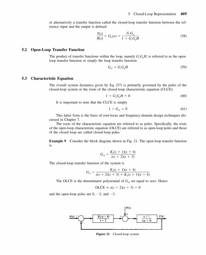
Example 9 Consider the block diagram shown in Fig. 21. The open-loop transfer functionis
K (s � 1)(s � 4)1G �ol s(s � 2)(s � 3)
The closed-loop transfer function of the system is
K (s � 1)(s � 4)1G �cl s(s � 2)(s � 3) � K (s � 1)(s � 4)1
The OLCE is the denominator polynomial of Gol set equal to zero. Hence
OLCE � s(s � 2)(s � 3) � 0
and the open-loop poles are 0, �2, and �3.
470 Closed-Loop Control System Analysis
The CLCE is
s(s � 2)(s � 3) � K (s � 1)(s � 4) � 01
and its roots are the closed-loop poles appropriate for the specific gain value K1.If the transfer functions are rational (i.e., are ratios of polynomials), then they can be
written as
mK (s � z )�i�1 iG(s) � (62)n (s � p )�j�1 j
When the poles of the transfer function G(s) are distinct, G(s) may be written in partial-fraction form as
n AjG(s) � (63)�
S � pj�1 j
Hence
n Aj�1 �1g(t) � L [G(s)] � L �� s � pj�1 j
n�p tj� A e (64)� j
j�1
Since a transfer function G(s) � L [output] / L [input], g(t) of of Eq. (64) is the response ofthe system depicted by G(s) for a unit impulse �(t), since L [�(t)] � 1.
The impulse response of a given system is key to its internal stability. The term systemhere is applicable to any part of (or the whole) closed-loop system.
It should be noted that the zeros of the transfer function only affect the residues Aj. Inother words, the contribution from the corresponding transient term may or may not be�p tjesignificant depending on the relative size of Aj. If, for instance, a zero �zk is very close toa pole �pl, then the transient term would have a value close to zero for its residue�p tjAeAl. As an example, consider the unit impulse response of the two systems:
1 1 1G (s) � � (65)1 (s � 1)(s � 2) s � 1 s � 2
(s � 1.05) 0.05 0.95G (s) � � � (66)2 (s � 1)(s � 2) s � 1 s � 2
From Eq. (65), g1(t) � e�t � e�2t, and from Eq. (66), g2(t) � 0.05e�t � 0.95e�2t.Note that the effect of the term e�t has been modified from a residue of 1 in G1 to a
residue of 0.05 in G2. This observation helps to reduce the order of a system when there arepoles and zeros close together. In G2(s), for example, little error would be introduced if thezero at �1.05 and the pole at �1 are neglected and the transfer function is approximatedby
1G (s) �2 s � 2
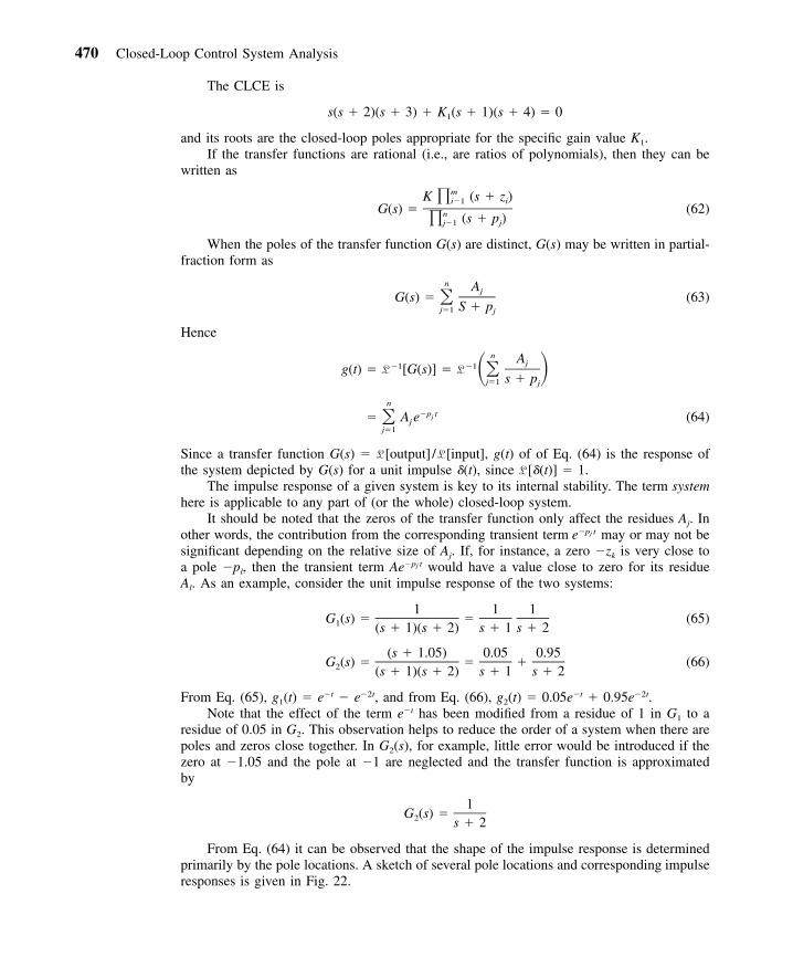
From Eq. (64) it can be observed that the shape of the impulse response is determinedprimarily by the pole locations. A sketch of several pole locations and corresponding impulseresponses is given in Fig. 22.
5 Closed-Loop Representation 471
Figure 22 Impulse responses associated with pole locations. LHP, RHP: left- and right-half plane.
The fundamental responses that can be obtained are of the form e��t and e�t sin �t with� � 0. It should be noted that for a real pole its location completely characterizes theresulting impulse response. When a transfer function has complex-conjugate poles, the im-pulse response is more complicated.
5.4 Standard Second-Order Transfer Function
A standard second-order transfer function takes the form
2� 1nG(s) � � (67)2 2 2 2s � 2�� s � � s /� � 2�(s /� ) � 1n n n n
Parameter � is called the damping ratio, and �n is called the undamped natural frequency.The poles of the transfer function given by Eq. (67) can be determined by solving its char-acteristic equation:
472 Closed-Loop Control System Analysis
Figure 23 Compelx-conjugate poles in the s-plane.
2 2s � 2�� s � � � 0 (68)n n
giving the poles
2s � ��� � j1 � � � � �� � j� (69)1.2 n n d
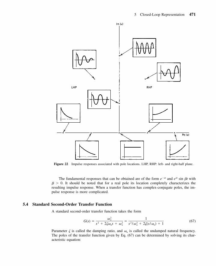
where � � ��n and �d � �n � � 1.21 � � ,The two complex-conjugate poles given by Eq. (69) are located in the complex s-plane,
as shown in Fig. 23.It can be easily seen that
2 2 2�s � � � � � � � � (70)1.2 n d n
and
1–cos � � � 0 � � � (71)2
When the system has no damping, � � 0, the impulse response is a pure sinusoidal oscil-lation. In this case the undamped natural frequency �n is equal to the damped natural fre-quency �d.
5.5 Step Input Response of a Standard Second-Order System
When the transfer function has complex-conjugate poles, the step input response rather thanthe impulse response is used to characterize its transients. Moreover, these transients arealmost always used as time-domain design specifications. The unit step input response ofthe second-order system given by Eq. (67) can be easily shown to be
5 Closed-Loop Representation 473
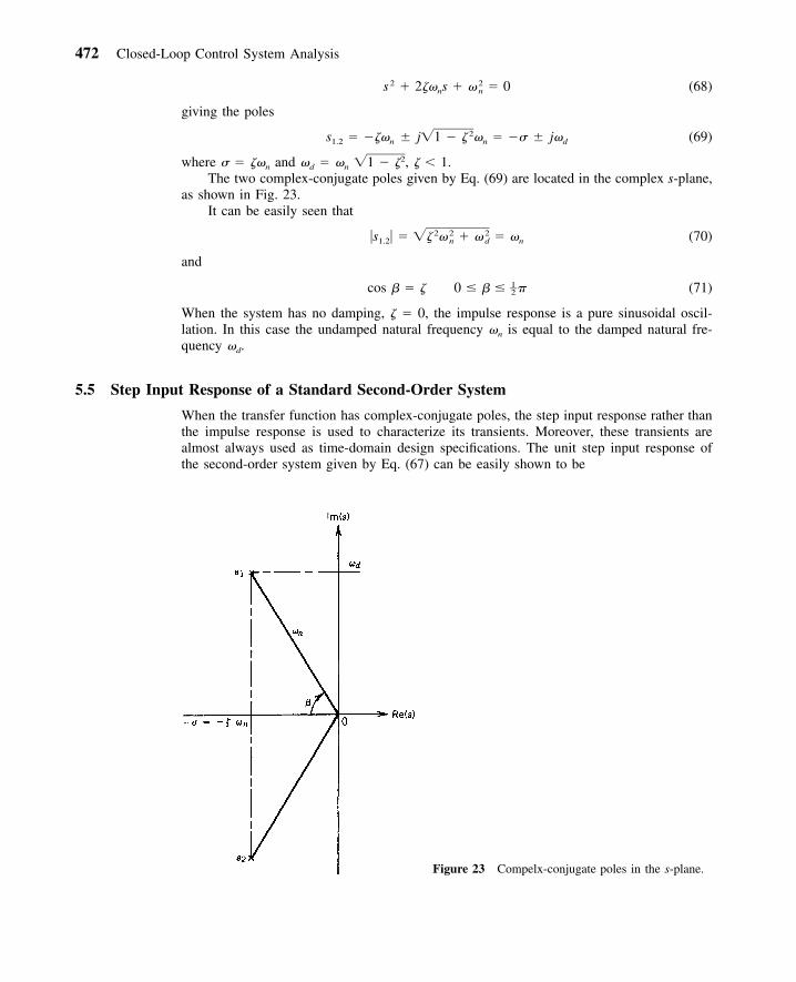
Figure 24 Definition of the rise time tr, settling time ts, and overshoot time Mp.
��Ty(t) � 1 � e cos � t � sin � t (72)� d d�d
where y(t) is the output.A typical unit step input response is shown in Fig. 24.From the time response of Eq. (72) several key parameters characterizing the shape of
the curve are usually used as time-domain design specifications. They are the rise time tr,the settling time ts, the peak overshoot Mp, and the peak time tp.
Rise Time tr
The time taken for the output to change from 10% of the steady-state value to 90% of thesteady-state value is usually called the rise time. There are other definitions of rise time.2
The basic idea, however, is that tr is a characterization of how rapid the system responds toan input.
A rule of thumb for tr is
1.8t (73)r �n
Settling Time ts
This is the time required for the transients to decay to a small value so that y(t) is almostat the steady-state level. Various measures of ‘‘smallness’’ are possible: 1, 2, and 5% aretypical.
4.6For 1% settling: t s ��n
4For 2% settling: t (74)s ��n
3For 5% settling: t s ��n
Peak Overshoot Mp
The peak overshoot is the maximum amount by which the output exceeds its steady-statevalue during the transients. It can be easily shown that
474 Closed-Loop Control System Analysis
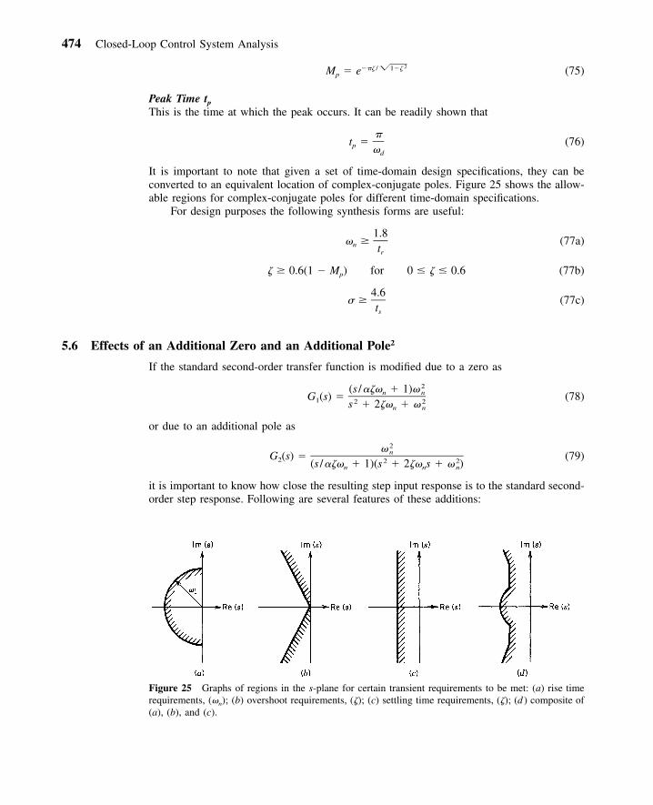
Figure 25 Graphs of regions in the s-plane for certain transient requirements to be met: (a) rise timerequirements, (�n); (b) overshoot requirements, (�); (c) settling time requirements, (�); (d ) composite of(a), (b), and (c).
2�� / 1��M � e (75)p
Peak Time tp
This is the time at which the peak occurs. It can be readily shown that
t � (76)p �d
It is important to note that given a set of time-domain design specifications, they can beconverted to an equivalent location of complex-conjugate poles. Figure 25 shows the allow-able regions for complex-conjugate poles for different time-domain specifications.
For design purposes the following synthesis forms are useful:
1.8� � (77a)n tr
� � 0.6(1 � M ) for 0 � � � 0.6 (77b)p
4.6� � (77c)
ts
5.6 Effects of an Additional Zero and an Additional Pole2
If the standard second-order transfer function is modified due to a zero as
2(s /��� � 1)�n nG (s) � (78)1 2 2s � 2�� � �n n
or due to an additional pole as
2� nG (s) � (79)2 2 2(s /��� � 1)(s � 2�� s � � )n n n
it is important to know how close the resulting step input response is to the standard second-order step response. Following are several features of these additions:
6 Stability 475
1. For a second-order system with no finite zeros, the transient parameters can beapproximated by Eq. (77).
2. An additional zero as in Eq. (78) in the left-half plane will increase the overshoot ifthe zero is within a factor of 4 of the real part of the complex poles. A plot is givenin Fig. 26.
3. An additional zero in the right-half plane will depress the overshoot (and may causethe step response to undershoot). This is referred to as a non-minimum-phase system.
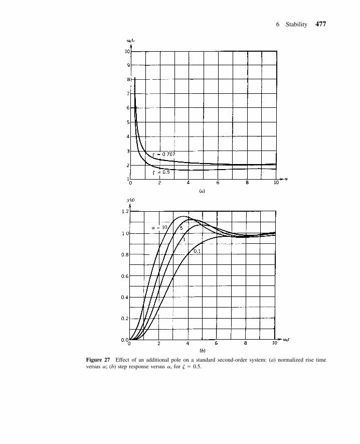
4. An additional pole in the left-half plane will increase the rise time significantly ifthe extra pole is within a factor of 4 of the real part of the complex poles. A plot isgiven in Fig. 27.
6 STABILITY
We shall distinguish between two types of stabilities: external and internal stability. Thenotion of external stability is concerned with whether or not a bounded input gives a boundedoutput. In this type of stability we notice that no reference is made to the internal variablesof the system. The implication here is that it is possible for an internal variable to growwithout bound while the output remains bounded. Whether or not the internal variables arewell behaved is typically addressed by the notion of internal stability. Internal stability re-quires that in the absence of an external input the internal variables stay bounded for anyperturbations of these variables. In other words internal stability is concerned with the re-sponse of the system due to nonzero initial conditions. It is reasonable to expect that a well-designed system should be both externally and internally stable.
The notion of asymptotic stability is usually discussed within the context of internalstability. Specifically, if the response due to nonzero initial conditions decays to zero as-ymptotically, then the system is said to be asymptotically stable. A LTI system is asymp-totically stable if and only if all the system poles lie in the open left-half-plane (i.e., theleft-half s-plane excluding the imaginary axis). This condition also guarantees external sta-bility for LTI systems. So in the case of LTI systems the notions of internal and externalstability may be considered equivalent.
For LTI systems, knowing the locations of the poles or the roots of the characteristicequation would suffice to predict stability. The Routh–Hurwitz stability criterion is frequentlyused to obtain stability information without explicitly computing the poles for LTI. Thiscriterion will be discussed in Section 6.1.
For nonlinear systems, stability cannot be characterized that easily. As a matter of fact,there are many definitions and theorems for assessing stability of such systems. A discussionof these topics is beyond the scope of this handbook. Interested reader may refer to Ref. 3.
6.1 Routh–Hurwitz Stability Criterion
This criterion allows one to predict the status of stability of a system by knowing the co-efficients of its characteristic polynomial. Consider the characteristic polynomial of an nth-order system:
n n�1 n�2P(s) � a s � a s � a s � � � � � a s � an n�1 n�2 1 0
A necessary condition for asymptotic stability is that all the coefficients {ai}’s be positive.If any of the coefficients are missing (i.e., are zero) or negative, then the system will have
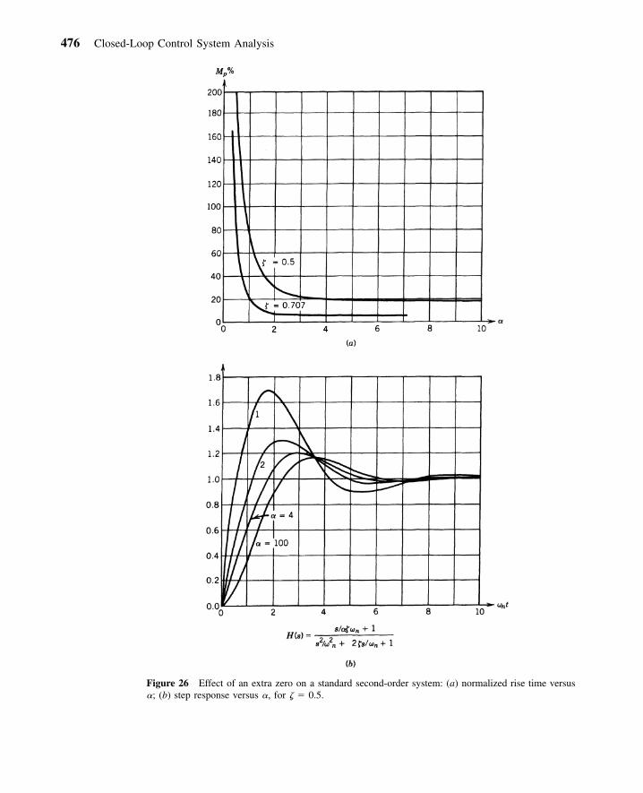
476 Closed-Loop Control System Analysis
Figure 26 Effect of an extra zero on a standard second-order system: (a) normalized rise time versus�; (b) step response versus �, for � � 0.5.
6 Stability 477
Figure 27 Effect of an additional pole on a standard second-order system: (a) normalized rise timeversus �; (b) step response versus �, for � � 0.5.
478 Closed-Loop Control System Analysis
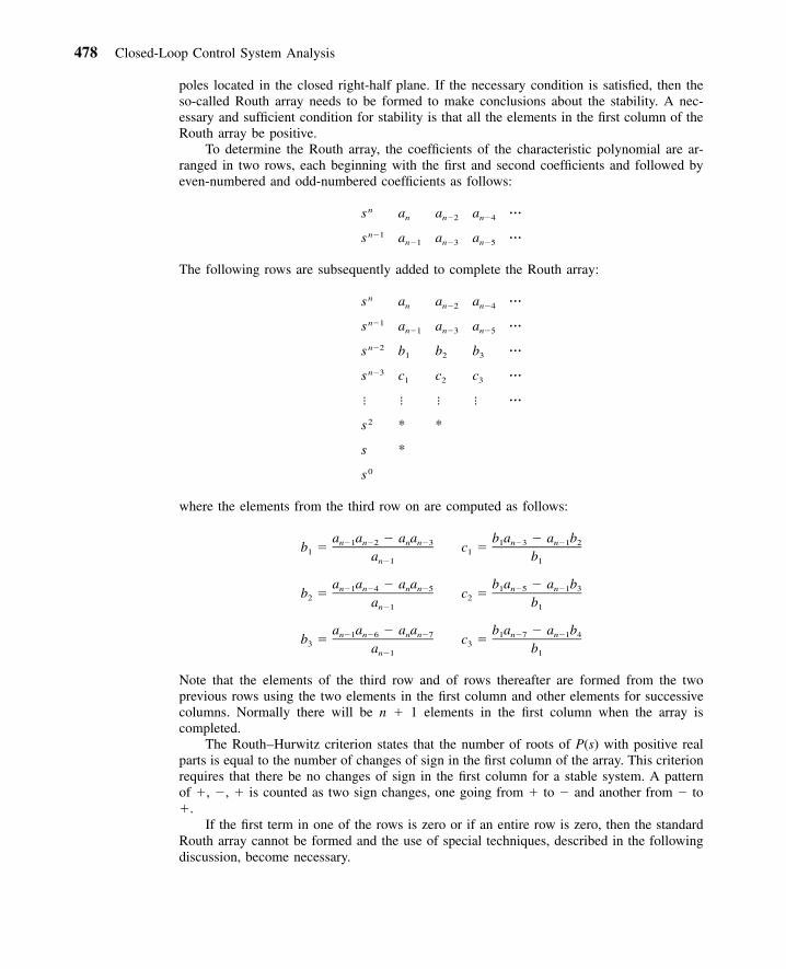
poles located in the closed right-half plane. If the necessary condition is satisfied, then theso-called Routh array needs to be formed to make conclusions about the stability. A nec-essary and sufficient condition for stability is that all the elements in the first column of theRouth array be positive.
To determine the Routh array, the coefficients of the characteristic polynomial are ar-ranged in two rows, each beginning with the first and second coefficients and followed byeven-numbered and odd-numbered coefficients as follows:
ns a a a � � �n n�2 n�4
n�1s a a a � � �n�1 n�3 n�5
The following rows are subsequently added to complete the Routh array:
ns a a a � � �n n�2 n�4
n�1s a a a � � �n�1 n�3 n�5
n�2s b b b � � �1 2 3
n�3s c c c � � �1 2 3
� � � � � � �
2s * *
s *
0s
where the elements from the third row on are computed as follows:
a a � a a b a � a bn�1 n�2 n n�3 1 n�3 n�1 2b � c �1 1a bn�1 1
a a � a a b a � a bn�1 n�4 n n�5 1 n�5 n�1 3b � c �2 2a bn�1 1
a a � a a b a � a bn�1 n�6 n n�7 1 n�7 n�1 4b � c �3 3a bn�1 1
Note that the elements of the third row and of rows thereafter are formed from the twoprevious rows using the two elements in the first column and other elements for successivecolumns. Normally there will be n � 1 elements in the first column when the array iscompleted.
The Routh–Hurwitz criterion states that the number of roots of P(s) with positive realparts is equal to the number of changes of sign in the first column of the array. This criterionrequires that there be no changes of sign in the first column for a stable system. A patternof �, �, � is counted as two sign changes, one going from � to � and another from � to�.
If the first term in one of the rows is zero or if an entire row is zero, then the standardRouth array cannot be formed and the use of special techniques, described in the followingdiscussion, become necessary.
6 Stability 479
Special Cases
1. Zero in the first column, while some other elements of the row containing a zero inthe first column are nonzero
2. Zero in the first column, and the other elements of the row containing the zero arealso zero
CASE 1: In this case the zero is replaced with a small positive constant � 0, and the arrayis completed as before. The stability criterion is then applied by taking the limits of entriesof the first column as → 0. For example, consider the following characteristic equation:
5 4 3 2s � 2s � 2s � 4s � 11s � 10 � 0
The Routh array is then
1 2 112 4 100 6 0 6 0 first column zero replaced by c 101
d 01
where
4 � 12 6c � 10 1c � and d �1 1 c1
As → 0, we get c1 �12/ , and d1 6. There are two sign changes due to the largenegative number in the first column. Therefore the system is unstable, and two roots lie inthe right-half plane. As a final example consider the characteristic polynomial
4 3 2P(s) � s � 5s � 7s � 5s � 6
The Routh array is
1 7 65 56 6 ← Zero replaced by � 06
If � 0, there are no sign changes. If � 0, there are two sign changes. Thus if � 0, itindicates that there are two roots on the imaginary axis, and a slight perturbation woulddrive the roots into the right-half plane or the left-half plane. An alternative procedure is todefine the auxiliary variable
1z �
s
and convert the characteristic polynomial so that it is in terms of z. This usually produces aRouth array with nonzero elements in the first column. The stability properties can then bededuced from this array.
480 Closed-Loop Control System Analysis
CASE 2: This case corresponds to a situation where the characteristic equation has equal andopposite roots. In this case if the ith row is the vanishing row, an auxiliary equation is formedfrom the previous i�1 row as follows:
i�1 i�1 i�3P (s) � � s � � s � � s � � � �1 1 2 3
where the {�i}’s are the coefficients of the (i � 1)th row of the array. The ith row is thenreplaced by the coefficients of the derivative of the auxiliary polynomial, and the array iscompleted. Moreover, the roots of the auxiliary polynomial are also roots of the characteristicequation. As an example, consider
5 4 3 2s � 2s � 5s � 10s � 4s � 8 � 0
for which the Routh array is
5s 1 5 44s 2 10 83 4 2s 0 0 Auxiliary equation: 2s � 10s � 8 � 03s 8 202s 5 81s 7.20s 8
There are no sign changes in the first column. Hence all the roots have nonpositive real partswith two pairs of roots on the imaginary axis, which are the roots of
4 22s � 10s � 8 � 0
2 2� 2(s � 4)(s � 1)
Thus equal and opposite roots indicated by the vanishing row are �j and �2j.The Routh–Hurwitz criterion may also be used in determining the range of parameters
for which a feedback system remains stable. Consider, for example, the system described bythe CLCE
4 3 2s � 3s � 3s � 2s � K � 0
The corresponding Routh array is
4s 1 3 K3s 3 2
72s K3
1s s � (9 /7)K0s K
If the system is to remain asymptotically stable, we must have
14––0 � K � 9
The Routh–Hurwitz stability criterion can also be used to obtain additional insights. Forinstance information regarding the speed of response may be obtained by a coordinate trans-formation of the form s � a, where �a characterizes rate. For this additional detail the readeris referred to Ref. 4.
6 Stability 481
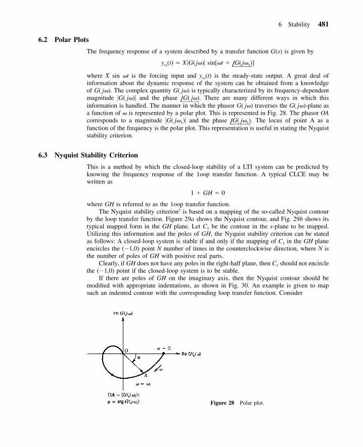
Figure 28 Polar plot.
6.2 Polar Plots
The frequency response of a system described by a transfer function G(s) is given by
y (t) � X �G( j�)� sin[�t � G( j� )]ss 1/where X sin �t is the forcing input and yss(t) is the steady-state output. A great deal ofinformation about the dynamic response of the system can be obtained from a knowledgeof G( j�). The complex quantity G( j�) is typically characterized by its frequency-dependentmagnitude �G( j�)� and the phase There are many different ways in which thisG( j�)./information is handled. The manner in which the phasor G( j�) traverses the G( j�)-plane asa function of � is represented by a polar plot. This is represented in Fig. 28. The phasor OAcorresponds to a magnitude �G( j�1)� and the phase The locus of point A as aG( j� ).1/function of the frequency is the polar plot. This representation is useful in stating the Nyquiststability criterion.
6.3 Nyquist Stability Criterion
This is a method by which the closed-loop stability of a LTI system can be predicted byknowing the frequency response of the 1oop transfer function. A typical CLCE may bewritten as
1 � GH � 0
where GH is referred to as the 1oop transfer function.The Nyquist stability criterion2 is based on a mapping of the so-called Nyquist contour
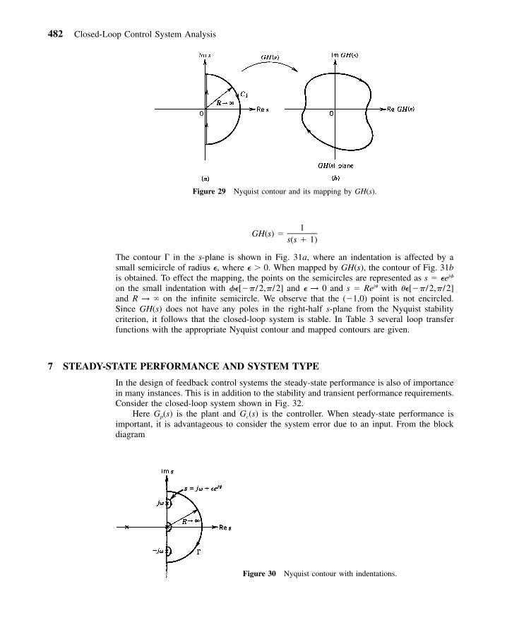
by the loop transfer function. Figure 29a shows the Nyquist contour, and Fig. 29b shows itstypical mapped form in the GH plane. Let C1 be the contour in the s-plane to be mapped.Utilizing this information and the poles of GH, the Nyquist stability criterion can be statedas follows: A closed-loop system is stable if and only if the mapping of C1 in the GH planeencircles the (�1,0) point N number of times in the counterclockwise direction, where N isthe number of poles of GH with positive real parts.
Clearly, if GH does not have any poles in the right-half plane, then C1 should not encirclethe (�1,0) point if the closed-loop system is to be stable.
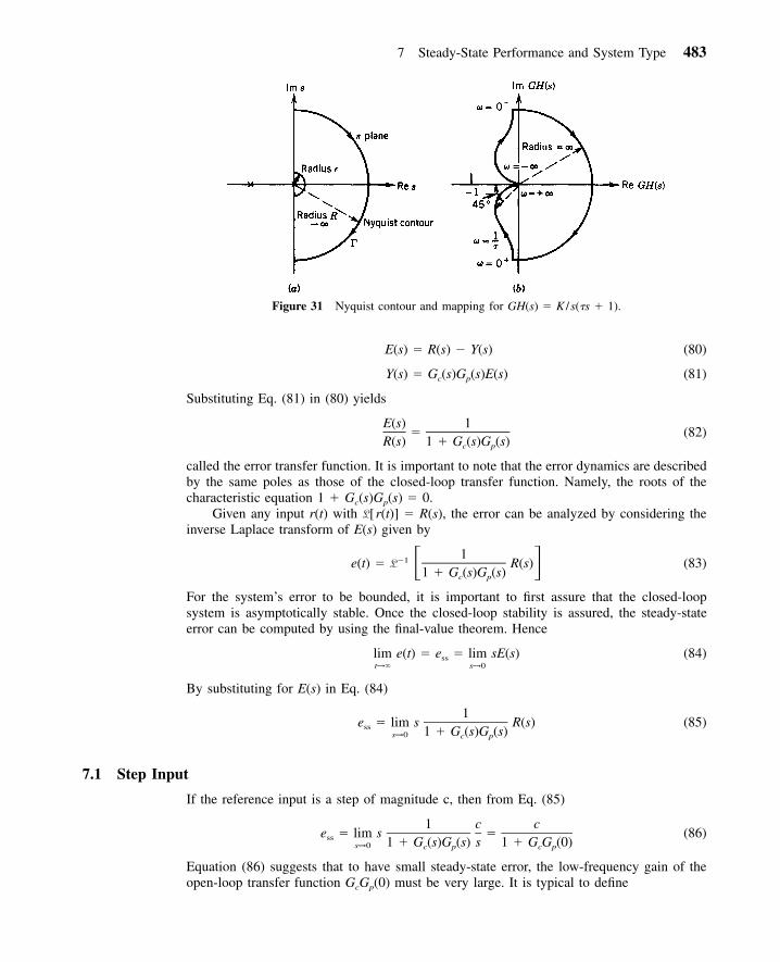
If there are poles of GH on the imaginary axis, then the Nyquist contour should bemodified with appropriate indentations, as shown in Fig. 30. An example is given to mapsuch an indented contour with the corresponding loop transfer function. Consider
482 Closed-Loop Control System Analysis
Figure 29 Nyquist contour and its mapping by GH(s).
Figure 30 Nyquist contour with indentations.
1GH(s) �
s(s � 1)
The contour � in the s-plane is shown in Fig. 31a, where an indentation is affected by asmall semicircle of radius , where � 0. When mapped by GH(s), the contour of Fig. 31bis obtained. To effect the mapping, the points on the semicircles are represented as s � ej
on the small indentation with [� /2, /2] and → 0 and s � Rej� with � [� /2, /2]and R → � on the infinite semicircle. We observe that the (�1,0) point is not encircled.Since GH(s) does not have any poles in the right-half s-plane from the Nyquist stabilitycriterion, it follows that the closed-loop system is stable. In Table 3 several loop transferfunctions with the appropriate Nyquist contour and mapped contours are given.
7 STEADY-STATE PERFORMANCE AND SYSTEM TYPE
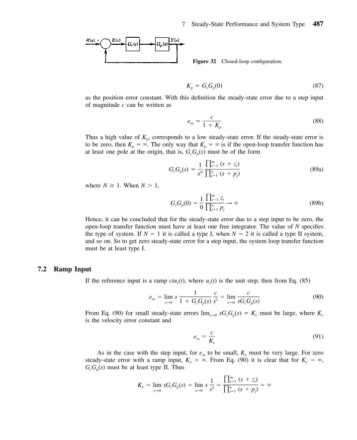
In the design of feedback control systems the steady-state performance is also of importancein many instances. This is in addition to the stability and transient performance requirements.Consider the closed-loop system shown in Fig. 32.
Here Gp(s) is the plant and Gc(s) is the controller. When steady-state performance isimportant, it is advantageous to consider the system error due to an input. From the blockdiagram
7 Steady-State Performance and System Type 483
Figure 31 Nyquist contour and mapping for GH(s) � K /s(�s � 1).
E(s) � R(s) � Y(s) (80)
Y(s) � G (s)G (s)E(s) (81)c p
Substituting Eq. (81) in (80) yields
E(s) 1� (82)
R(s) 1 � G (s)G (s)c p
called the error transfer function. It is important to note that the error dynamics are describedby the same poles as those of the closed-loop transfer function. Namely, the roots of thecharacteristic equation 1 � Gc(s)Gp(s) � 0.
Given any input r(t) with L[r(t)] � R(s), the error can be analyzed by considering theinverse Laplace transform of E(s) given by
1�1e(t) � L R(s) (83)� �1 � G (s)G (s)c p
For the system’s error to be bounded, it is important to first assure that the closed-loopsystem is asymptotically stable. Once the closed-loop stability is assured, the steady-stateerror can be computed by using the final-value theorem. Hence
lim e(t) � e � lim sE(s) (84)sst→� s→0
By substituting for E(s) in Eq. (84)
1e � lim s R(s) (85)ss 1 � G (s)G (s)s→0 c p
7.1 Step Input
If the reference input is a step of magnitude c, then from Eq. (85)
1 c ce � lim s � (86)ss 1 � G (s)G (s) s 1 � G G (0)s→0 c p c p
Equation (86) suggests that to have small steady-state error, the low-frequency gain of theopen-loop transfer function GcGp(0) must be very large. It is typical to define
484 Closed-Loop Control System Analysis
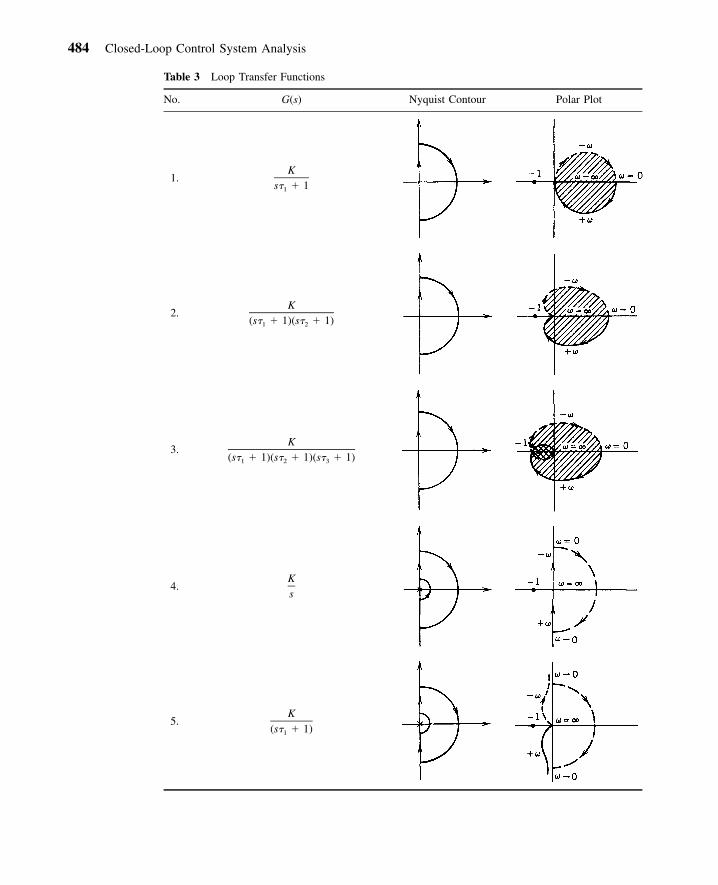
Table 3 Loop Transfer Functions
No. G(s) Nyquist Contour Polar Plot
1.K
s� � 11
2.K
(s� � 1)(s� � 1)1 2
3.K
(s� � 1)(s� � 1)(s� � 1)1 2 3
4.Ks
5.K
(s� � 1)1
7 Steady-State Performance and System Type 485
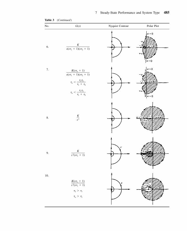
Table 3 (Continued )
No. G(s) Nyquist Contour Polar Plot
6.K
s(s� � 1)(s� � 1)1 2
7. K(s� � 1)a
s(s� � 1)(s� � 1)1 2
� �1 2� �a � � �1 2
� �1 2� �a � � �1 2
8.K
2s
9.K
2s (s� � 1)1
10.
K(s� � 1)12s (s� � 1)1
�2 � �1
�a � �1
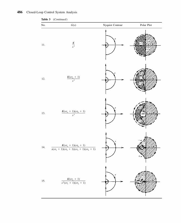
486 Closed-Loop Control System Analysis
Table 3 (Continued )
No. G(s) Nyquist Contour Polar Plot
11.K
3s
12.K(s� � 1)a
3s
13.K(s� � 1)(s� � 1)a b
3s
14.K(s� � 1)(s� � 1)a b
s(s� � 1)(s� � 1)(s� � 1)(s� � 1)1 2 3 4
15.K(s� � 1)a
2s (s� � 1)(s� � 1)1 2
7 Steady-State Performance and System Type 487
Figure 32 Closed-loop configuration.
K � G G (0) (87)p c p
as the position error constant. With this definition the steady-state error due to a step inputof magnitude c can be written as
ce � (88)ss 1 � Kp
Thus a high value of Kp, corresponds to a low steady-state error. If the steady-state error isto be zero, then Kp � �. The only way that Kp � � is if the open-loop transfer function hasat least one pole at the origin, that is, GcGp(s) must be of the form
m (s � z )�i�1 i1G G (s) � (89a)c p nNs (s � p )�j�1 j
where N � 1. When N � 1,
m z�i�1 i1G G (0) � → � (89b)c p n0 p�j�1 j
Hence, it can be concluded that for the steady-state error due to a step input to be zero, theopen-loop transfer function must have at least one free integrator. The value of N specifiesthe type of system. If N � 1 it is called a type I, when N � 2 it is called a type II system,and so on. So to get zero steady-state error for a step input, the system loop transfer functionmust be at least type I.
7.2 Ramp Input
If the reference input is a ramp ctus(t), where us(t) is the unit step, then from Eq. (85)
1 c ce � lim s � lim (90)ss 21 � G G (s) s sG G (s)s→0 s→0c p c p
From Eq. (90) for small steady-state errors lims→0 sGcGp(s) � Kv must be large, where Kv
is the velocity error constant and
ce � (91)ss Kv
As in the case with the step input, for ess to be small, Kv must be very large. For zerosteady-state error with a ramp input, Kv � �. From Eq. (90) it is clear that for Kv � �,GcGp(s) must be at least type II. Thus
m (s � z )�i�1 i1K � lim sG G (s) � lim s � � �v c p n2s (s � p )�s→0 s→0 j�1 j
488 Closed-Loop Control System Analysis
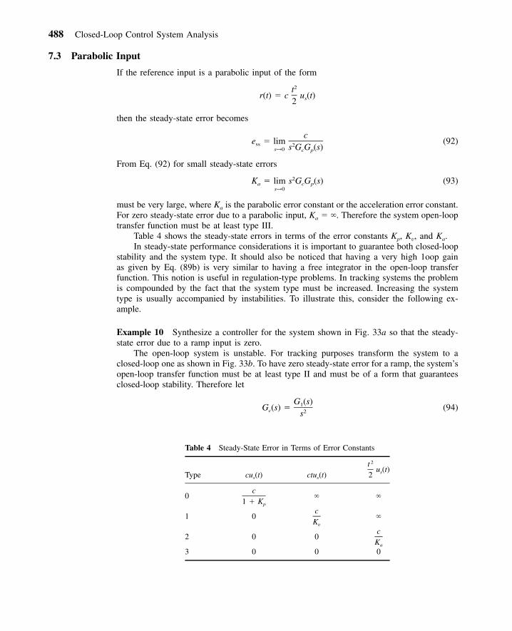
Table 4 Steady-State Error in Terms of Error Constants
Type cus(t) ctus(t)
2tu (t)s2
0c
1 � Kp
� �
1 0c
Kv
�
2 0 0c
Ka
3 0 0 0
7.3 Parabolic Input
If the reference input is a parabolic input of the form
2tr(t) � c u (t)s2
then the steady-state error becomes
ce � lim (92)ss 2s G G (s)s→0 c p
From Eq. (92) for small steady-state errors
2K � lim s G G (s) (93)a c ps→0
must be very large, where Ka is the parabolic error constant or the acceleration error constant.For zero steady-state error due to a parabolic input, Ka � �. Therefore the system open-looptransfer function must be at least type III.
Table 4 shows the steady-state errors in terms of the error constants Kp, Kv, and Ka.In steady-state performance considerations it is important to guarantee both closed-loop
stability and the system type. It should also be noticed that having a very high 1oop gainas given by Eq. (89b) is very similar to having a free integrator in the open-loop transferfunction. This notion is useful in regulation-type problems. In tracking systems the problemis compounded by the fact that the system type must be increased. Increasing the systemtype is usually accompanied by instabilities. To illustrate this, consider the following ex-ample.
Example 10 Synthesize a controller for the system shown in Fig. 33a so that the steady-state error due to a ramp input is zero.
The open-loop system is unstable. For tracking purposes transform the system to aclosed-loop one as shown in Fig. 33b. To have zero steady-state error for a ramp, the system’sopen-loop transfer function must be at least type II and must be of a form that guaranteesclosed-loop stability. Therefore let
G (s)1G (s) � (94)c 2s
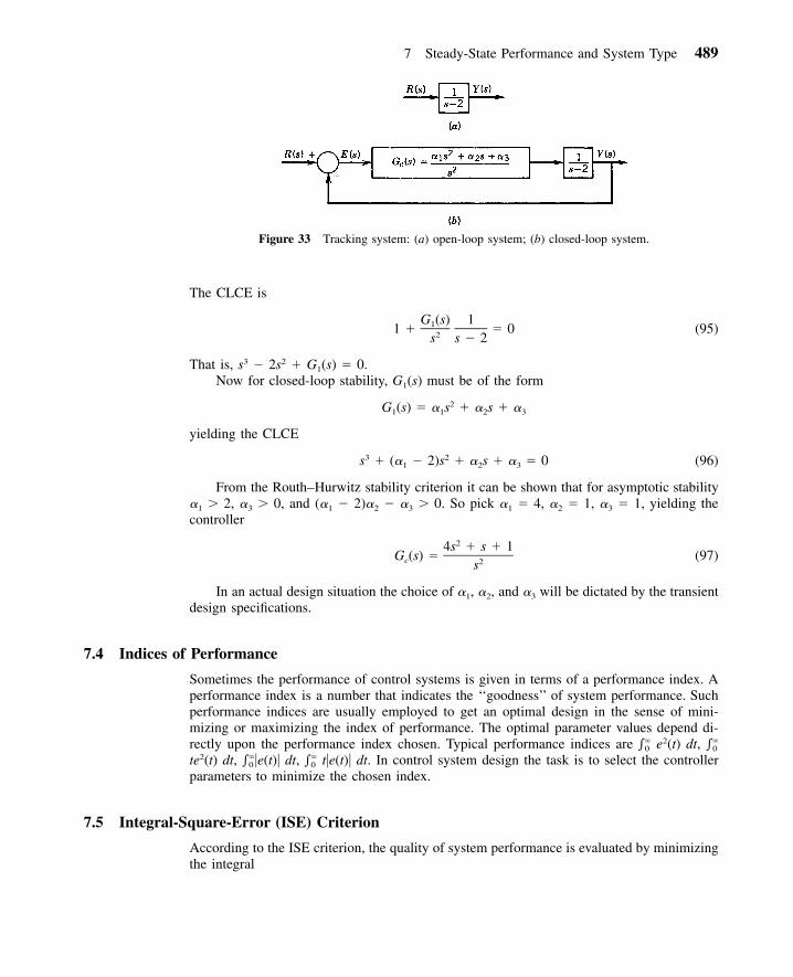
7 Steady-State Performance and System Type 489
Figure 33 Tracking system: (a) open-loop system; (b) closed-loop system.
The CLCE is
G (s) 111 � � 0 (95)2s s � 2
That is, s3 � 2s2 � G1(s) � 0.Now for closed-loop stability, G1(s) must be of the form
2G (s) � � s � � s � �1 1 2 3
yielding the CLCE
3 2s � (� � 2)s � � s � � � 0 (96)1 2 3
From the Routh–Hurwitz stability criterion it can be shown that for asymptotic stability�1 � 2, �3 � 0, and (�1 � 2)�2 � �3 � 0. So pick �1 � 4, �2 � 1, �3 � 1, yielding thecontroller
24s � s � 1G (s) � (97)c 2s
In an actual design situation the choice of �1, �2, and �3 will be dictated by the transientdesign specifications.
7.4 Indices of Performance
Sometimes the performance of control systems is given in terms of a performance index. Aperformance index is a number that indicates the ‘‘goodness’’ of system performance. Suchperformance indices are usually employed to get an optimal design in the sense of mini-mizing or maximizing the index of performance. The optimal parameter values depend di-rectly upon the performance index chosen. Typical performance indices are e2(t) dt,� �� �0 0
te2(t) dt, �e(t)� dt, t�e(t)� dt. In control system design the task is to select the controller� �� �0 0
parameters to minimize the chosen index.
7.5 Integral-Square-Error (ISE) Criterion
According to the ISE criterion, the quality of system performance is evaluated by minimizingthe integral
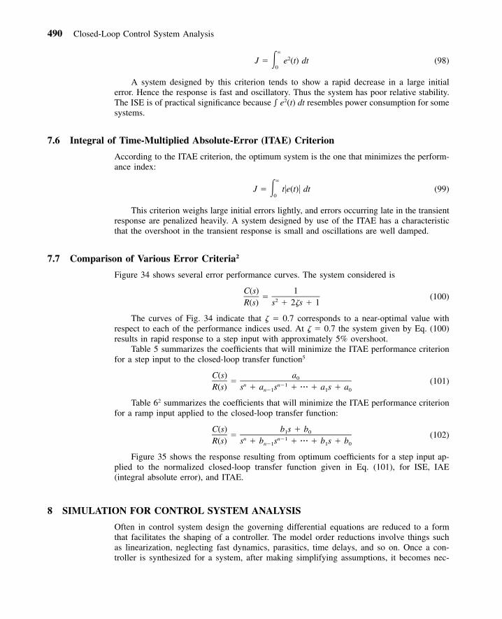
490 Closed-Loop Control System Analysis
�2J � � e (t) dt (98)
0
A system designed by this criterion tends to show a rapid decrease in a large initialerror. Hence the response is fast and oscillatory. Thus the system has poor relative stability.The ISE is of practical significance because � e2(t) dt resembles power consumption for somesystems.
7.6 Integral of Time-Multiplied Absolute-Error (ITAE) Criterion
According to the ITAE criterion, the optimum system is the one that minimizes the perform-ance index:
�
J � � t�e(t)� dt (99)0
This criterion weighs large initial errors lightly, and errors occurring late in the transientresponse are penalized heavily. A system designed by use of the ITAE has a characteristicthat the overshoot in the transient response is small and oscillations are well damped.
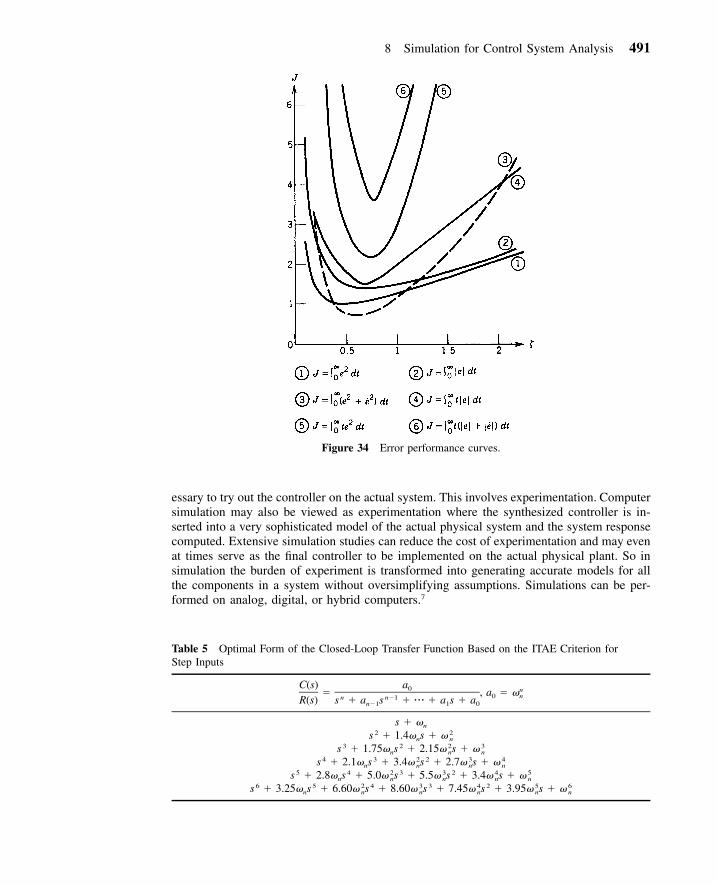
7.7 Comparison of Various Error Criteria2
Figure 34 shows several error performance curves. The system considered is
C(s) 1� (100)2R(s) s � 2�s � 1
The curves of Fig. 34 indicate that � � 0.7 corresponds to a near-optimal value withrespect to each of the performance indices used. At � � 0.7 the system given by Eq. (100)results in rapid response to a step input with approximately 5% overshoot.
Table 5 summarizes the coefficients that will minimize the ITAE performance criterionfor a step input to the closed-loop transfer function5
C(s) a0� (101)n n�1R(s) s � a s � � � � � a s � an�1 1 0
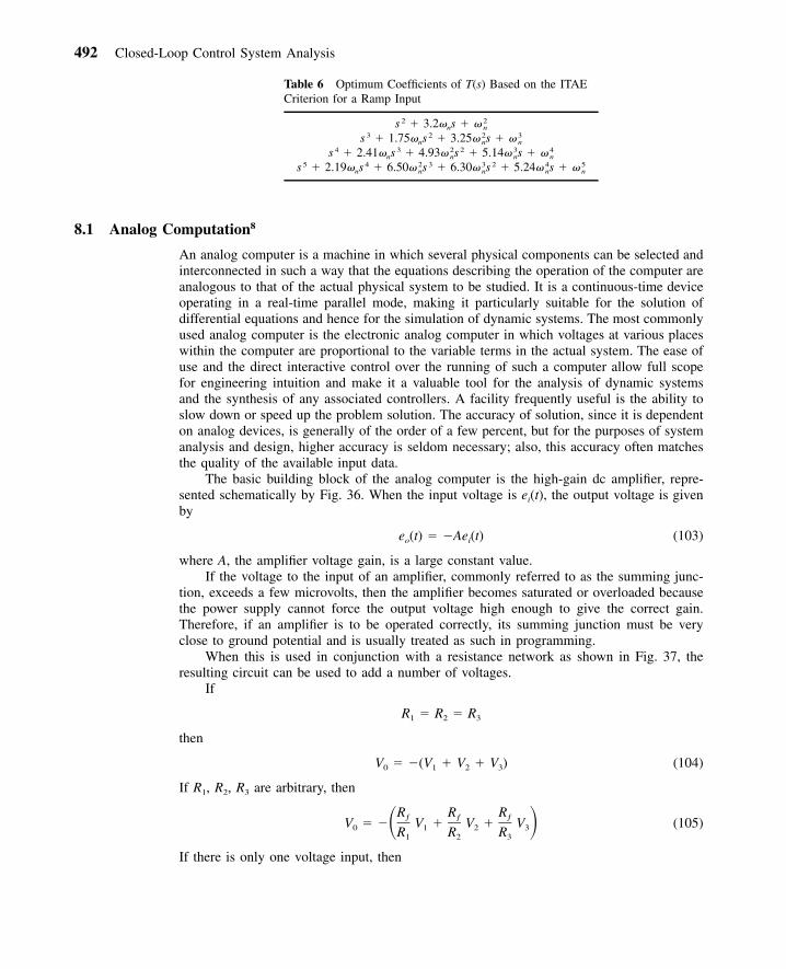
Table 62 summarizes the coefficients that will minimize the ITAE performance criterionfor a ramp input applied to the closed-loop transfer function:
C(s) b s � b1 0� (102)n n�1R(s) s � b s � � � � � b s � bn�1 1 0
Figure 35 shows the response resulting from optimum coefficients for a step input ap-plied to the normalized closed-loop transfer function given in Eq. (101), for ISE, IAE(integral absolute error), and ITAE.
8 SIMULATION FOR CONTROL SYSTEM ANALYSIS
Often in control system design the governing differential equations are reduced to a formthat facilitates the shaping of a controller. The model order reductions involve things suchas linearization, neglecting fast dynamics, parasitics, time delays, and so on. Once a con-troller is synthesized for a system, after making simplifying assumptions, it becomes nec-
8 Simulation for Control System Analysis 491
Figure 34 Error performance curves.
Table 5 Optimal Form of the Closed-Loop Transfer Function Based on the ITAE Criterion forStep Inputs
C(s) a0 n� , a � �0 nn n�1R(s) s � a s � � � � � a s � an�1 1 0
s � �n2 2s � 1.4� s � �n n
3 2 2 3s � 1.75� s � 2.15� s � �n n n4 3 2 2 3 4s � 2.1� s � 3.4� s � 2.7� s � �n n n n
5 4 2 3 3 2 4 5s � 2.8� s � 5.0� s � 5.5� s � 3.4� s � �n n n n n6 5 2 4 3 3 4 2 5 6s � 3.25� s � 6.60� s � 8.60� s � 7.45� s � 3.95� s � �n n n n n n
essary to try out the controller on the actual system. This involves experimentation. Computersimulation may also be viewed as experimentation where the synthesized controller is in-serted into a very sophisticated model of the actual physical system and the system responsecomputed. Extensive simulation studies can reduce the cost of experimentation and may evenat times serve as the final controller to be implemented on the actual physical plant. So insimulation the burden of experiment is transformed into generating accurate models for allthe components in a system without oversimplifying assumptions. Simulations can be per-formed on analog, digital, or hybrid computers.7
492 Closed-Loop Control System Analysis
Table 6 Optimum Coefficients of T(s) Based on the ITAECriterion for a Ramp Input
2 2s � 3.2� s � �n n3 2 2 3s � 1.75� s � 3.25� s � �n n n
4 3 2 2 3 4s � 2.41� s � 4.93� s � 5.14� s � �n n n n5 4 2 3 3 2 4 5s � 2.19� s � 6.50� s � 6.30� s � 5.24� s � �n n n n n
8.1 Analog Computation8
An analog computer is a machine in which several physical components can be selected andinterconnected in such a way that the equations describing the operation of the computer areanalogous to that of the actual physical system to be studied. It is a continuous-time deviceoperating in a real-time parallel mode, making it particularly suitable for the solution ofdifferential equations and hence for the simulation of dynamic systems. The most commonlyused analog computer is the electronic analog computer in which voltages at various placeswithin the computer are proportional to the variable terms in the actual system. The ease ofuse and the direct interactive control over the running of such a computer allow full scopefor engineering intuition and make it a valuable tool for the analysis of dynamic systemsand the synthesis of any associated controllers. A facility frequently useful is the ability toslow down or speed up the problem solution. The accuracy of solution, since it is dependenton analog devices, is generally of the order of a few percent, but for the purposes of systemanalysis and design, higher accuracy is seldom necessary; also, this accuracy often matchesthe quality of the available input data.
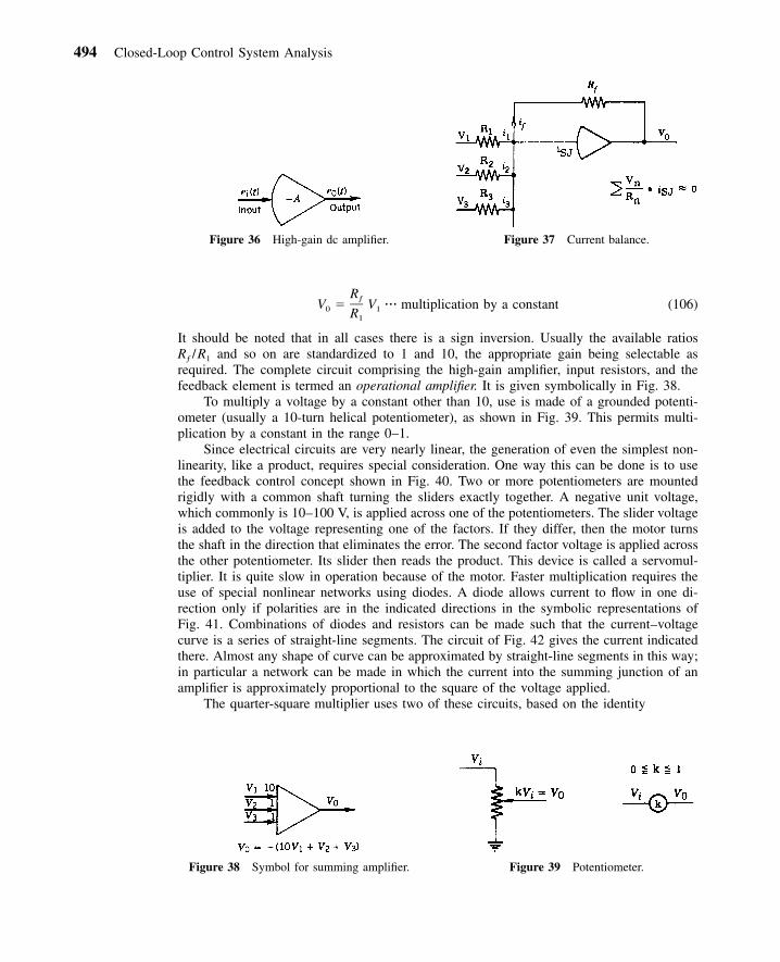
The basic building block of the analog computer is the high-gain dc amplifier, repre-sented schematically by Fig. 36. When the input voltage is ei(t), the output voltage is givenby
e (t) � �Ae (t) (103)o i
where A, the amplifier voltage gain, is a large constant value.If the voltage to the input of an amplifier, commonly referred to as the summing junc-
tion, exceeds a few microvolts, then the amplifier becomes saturated or overloaded becausethe power supply cannot force the output voltage high enough to give the correct gain.Therefore, if an amplifier is to be operated correctly, its summing junction must be veryclose to ground potential and is usually treated as such in programming.
When this is used in conjunction with a resistance network as shown in Fig. 37, theresulting circuit can be used to add a number of voltages.
If
R � R � R1 2 3
then
V � �(V � V � V ) (104)0 1 2 3
If R1, R2, R3 are arbitrary, then
R R Rƒ ƒ ƒV � � V � V � V (105)� 0 1 2 3R R R1 2 3
If there is only one voltage input, then

493
Figure 35 (a) Step response of a normalized transfer function using optimum coefficients of ISE, (b)IAE, and (c) ITAE.
494 Closed-Loop Control System Analysis
Figure 36 High-gain dc amplifier. Figure 37 Current balance.
Figure 38 Symbol for summing amplifier. Figure 39 Potentiometer.
RƒV � V � � � multiplication by a constant (106)0 1R1
It should be noted that in all cases there is a sign inversion. Usually the available ratiosRƒ /R1 and so on are standardized to 1 and 10, the appropriate gain being selectable asrequired. The complete circuit comprising the high-gain amplifier, input resistors, and thefeedback element is termed an operational amplifier. It is given symbolically in Fig. 38.
To multiply a voltage by a constant other than 10, use is made of a grounded potenti-ometer (usually a 10-turn helical potentiometer), as shown in Fig. 39. This permits multi-plication by a constant in the range 0–1.
Since electrical circuits are very nearly linear, the generation of even the simplest non-linearity, like a product, requires special consideration. One way this can be done is to usethe feedback control concept shown in Fig. 40. Two or more potentiometers are mountedrigidly with a common shaft turning the sliders exactly together. A negative unit voltage,which commonly is 10–100 V, is applied across one of the potentiometers. The slider voltageis added to the voltage representing one of the factors. If they differ, then the motor turnsthe shaft in the direction that eliminates the error. The second factor voltage is applied acrossthe other potentiometer. Its slider then reads the product. This device is called a servomul-tiplier. It is quite slow in operation because of the motor. Faster multiplication requires theuse of special nonlinear networks using diodes. A diode allows current to flow in one di-rection only if polarities are in the indicated directions in the symbolic representations ofFig. 41. Combinations of diodes and resistors can be made such that the current–voltagecurve is a series of straight-line segments. The circuit of Fig. 42 gives the current indicatedthere. Almost any shape of curve can be approximated by straight-line segments in this way;in particular a network can be made in which the current into the summing junction of anamplifier is approximately proportional to the square of the voltage applied.
The quarter-square multiplier uses two of these circuits, based on the identity
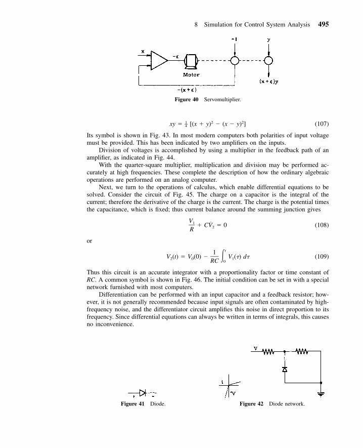
8 Simulation for Control System Analysis 495
Figure 40 Servomultiplier.
Figure 41 Diode. Figure 42 Diode network.
1 2 2–xy � [(x � y) � (x � y) ] (107)4
Its symbol is shown in Fig. 43. In most modern computers both polarities of input voltagemust be provided. This has been indicated by two amplifiers on the inputs.
Division of voltages is accomplished by using a multiplier in the feedback path of anamplifier, as indicated in Fig. 44.
With the quarter-square multiplier, multiplication and division may be performed ac-curately at high frequencies. These complete the description of how the ordinary algebraicoperations are performed on an analog computer.
Next, we turn to the operations of calculus, which enable differential equations to besolved. Consider the circuit of Fig. 45. The charge on a capacitor is the integral of thecurrent; therefore the derivative of the charge is the current. The charge is the potential timesthe capacitance, which is fixed; thus current balance around the summing junction gives
V1 ˙� CV � 0 (108)2R
or
t1V (t) � V (0) � � V (�) d� (109)2 0 1
0RC
Thus this circuit is an accurate integrator with a proportionality factor or time constant ofRC. A common symbol is shown in Fig. 46. The initial condition can be set in with a specialnetwork furnished with most computers.
Differentiation can be performed with an input capacitor and a feedback resistor; how-ever, it is not generally recommended because input signals are often contaminated by high-frequency noise, and the differentiator circuit amplifies this noise in direct proportion to itsfrequency. Since differential equations can always be written in terms of integrals, this causesno inconvenience.
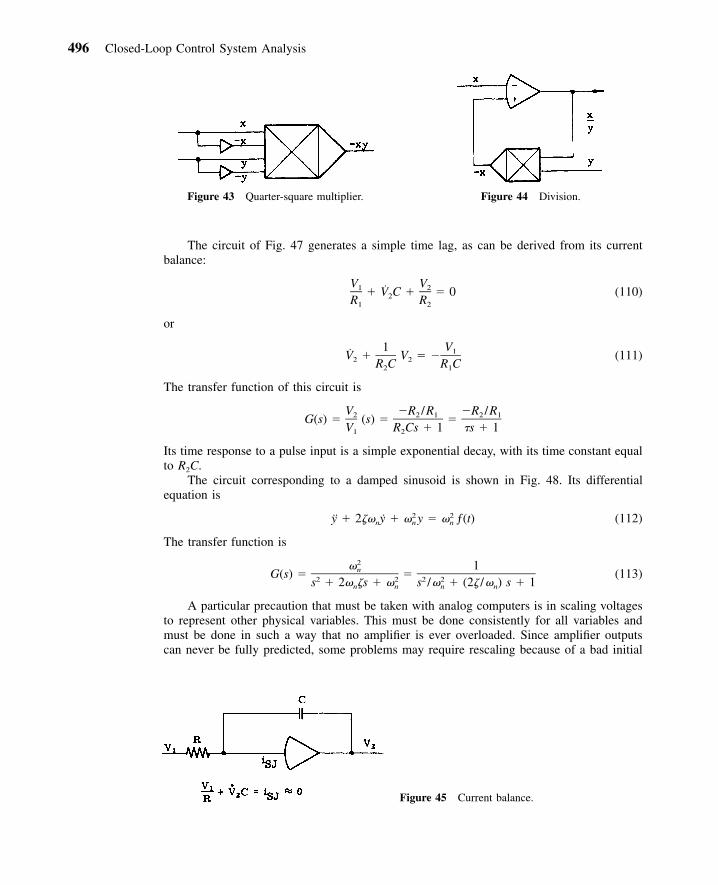
496 Closed-Loop Control System Analysis
Figure 43 Quarter-square multiplier. Figure 44 Division.
Figure 45 Current balance.
The circuit of Fig. 47 generates a simple time lag, as can be derived from its currentbalance:
V V1 2˙� V C � � 0 (110)2R R1 2
or
1 V1V � V � � (111)2 2R C R C2 1
The transfer function of this circuit is
V �R /R �R /R2 2 1 2 1G(s) � (s) � �V R Cs � 1 �s � 11 2
Its time response to a pulse input is a simple exponential decay, with its time constant equalto R2C.
The circuit corresponding to a damped sinusoid is shown in Fig. 48. Its differentialequation is
2 2y � 2�� y � � y � � ƒ(t) (112)n n n
The transfer function is
2� 1nG(s) � � (113)2 2 2 2s � 2� �s � � s /� � (2� /� ) s � 1n n n n
A particular precaution that must be taken with analog computers is in scaling voltagesto represent other physical variables. This must be done consistently for all variables andmust be done in such a way that no amplifier is ever overloaded. Since amplifier outputscan never be fully predicted, some problems may require rescaling because of a bad initial
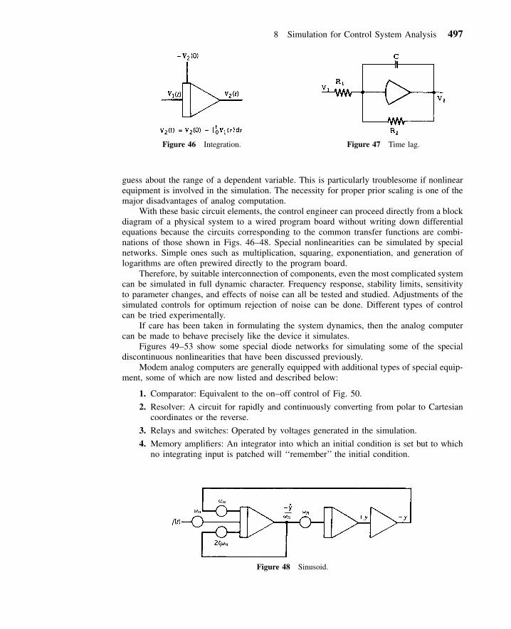
8 Simulation for Control System Analysis 497
Figure 46 Integration. Figure 47 Time lag.
Figure 48 Sinusoid.
guess about the range of a dependent variable. This is particularly troublesome if nonlinearequipment is involved in the simulation. The necessity for proper prior scaling is one of themajor disadvantages of analog computation.
With these basic circuit elements, the control engineer can proceed directly from a blockdiagram of a physical system to a wired program board without writing down differentialequations because the circuits corresponding to the common transfer functions are combi-nations of those shown in Figs. 46–48. Special nonlinearities can be simulated by specialnetworks. Simple ones such as multiplication, squaring, exponentiation, and generation oflogarithms are often prewired directly to the program board.
Therefore, by suitable interconnection of components, even the most complicated systemcan be simulated in full dynamic character. Frequency response, stability limits, sensitivityto parameter changes, and effects of noise can all be tested and studied. Adjustments of thesimulated controls for optimum rejection of noise can be done. Different types of controlcan be tried experimentally.
If care has been taken in formulating the system dynamics, then the analog computercan be made to behave precisely like the device it simulates.
Figures 49–53 show some special diode networks for simulating some of the specialdiscontinuous nonlinearities that have been discussed previously.
Modem analog computers are generally equipped with additional types of special equip-ment, some of which are now listed and described below:
1. Comparator: Equivalent to the on–off control of Fig. 50.
2. Resolver: A circuit for rapidly and continuously converting from polar to Cartesiancoordinates or the reverse.
3. Relays and switches: Operated by voltages generated in the simulation.
4. Memory amplifiers: An integrator into which an initial condition is set but to whichno integrating input is patched will ‘‘remember’’ the initial condition.
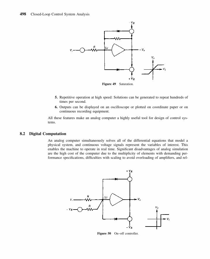
498 Closed-Loop Control System Analysis
Figure 49 Saturation.
Figure 50 On–off controller.
5. Repetitive operation at high speed: Solutions can be generated to repeat hundreds oftimes per second.
6. Outputs can be displayed on an oscilloscope or plotted on coordinate paper or oncontinuous recording equipment.
All these features make an analog computer a highly useful tool for design of control sys-tems.
8.2 Digital Computation
An analog computer simultaneously solves all of the differential equations that model aphysical system, and continuous voltage signals represent the variables of interest. Thisenables the machine to operate in real time. Significant disadvantages of analog simulationare the high cost of the computer due to the multiplicity of elements with demanding per-formance specifications, difficulties with scaling to avoid overloading of amplifiers, and rel-
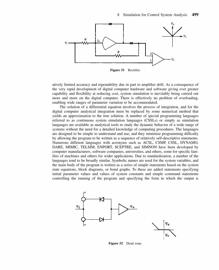
8 Simulation for Control System Analysis 499
Figure 51 Rectifier.
Figure 52 Dead zone.
atively limited accuracy and repeatability due in part to amplifier drift. As a consequence ofthe very rapid development of digital computer hardware and software giving ever greatercapability and flexibility at reducing cost, system simulation is inevitably being carried outmore and more on the digital computer. There is effectively no problem of overloading,enabling wide ranges of parameter variation to be accommodated.
The solution of a differential equation involves the process of integration, and for thedigital computer analytical integration must be replaced by some numerical method thatyields an approximation to the true solution. A number of special programming languagesreferred to as continuous system simulation languages (CSSLs) or simply as simulationlanguages are available as analytical tools to study the dynamic behavior of a wide range ofsystems without the need for a detailed knowledge of computing procedures. The languagesare designed to be simple to understand and use, and they minimize programming difficultyby allowing the program to be written as a sequence of relatively self-descriptive statements.Numerous different languages with acronyms such as ACSL, CSMP, CSSL, DYNAMO,DARE, MIMIC, TELSIM, ENPORT, SCEPTRE, and SIMNON have been developed bycomputer manufacturers, software companies, universities, and others, some for specific fam-ilies of machines and others for wider applications. Due to standardization, a number of thelanguages tend to be broadly similar. Symbolic names are used for the system variables, andthe main body of the program is written as a series of simple statements based on the systemstate equations, block diagrams, or bond graphs. To these are added statements specifyinginitial parameter values and values of system constants and simple command statementscontrolling the running of the program and specifying the form in which the output is
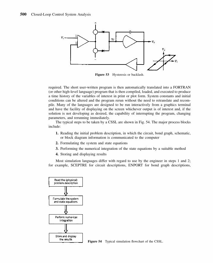
500 Closed-Loop Control System Analysis
Figure 53 Hysteresis or backlash.
Figure 54 Typical simulation flowchart of the CSSL.
required. The short user-written program is then automatically translated into a FORTRAN(or other high-level language) program that is then compiled, loaded, and executed to producea time history of the variables of interest in print or plot form. System constants and initialconditions can be altered and the program rerun without the need to retranslate and recom-pile. Many of the languages are designed to be run interactively from a graphics terminaland have the facility of displaying on the screen whichever output is of interest and, if thesolution is not developing as desired, the capability of interrupting the program, changingparameters, and rerunning immediately.
The typical steps to be taken by a CSSL are shown in Fig. 54. The major process blocksinclude:
1. Reading the initial problem description, in which the circuit, bond graph, schematic,or block diagram information is communicated to the computer
2. Formulating the system and state equations
3. Performing the numerical integration of the state equations by a suitable method
4. Storing and displaying results
Most simulation languages differ with regard to use by the engineer in steps 1 and 2;for example, SCEPTRE for circuit descriptions, ENPORT for bond graph descriptions,

Bibliography 501
CSMP for block diagrams, and DARE for state equations. The best guide to a program’scharacteristics is its user’s manual.
In summary, the advantages of digital simulation are (i) simple program writing, (ii)accuracy and reproducibility, (iii) cost-effectiveness, (iv) where interactive facilities exist,keyboard entry of program and running, (v) inspection of plots on graphics display screen,and (vi) online modification and rerunning.
8.3 Hybrid Computation
Hybrid computation is a combination of analog and digital computations. In hybrid com-putations analog and digital machines are used in such a way that a problem can be pro-grammed by exploiting the most efficient features of each. Much of the cost of such amachine arises from the rather complicated interface equipment required to make the nec-essary conversions between analog and digital signals and vice versa. The cost of an analogor hybrid computer is now justified only for certain large simulations where fast computingspeed attained by parallel operation is important. Even this advantage may disappear asparallel computation is introduced into digital systems.
REFERENCES
1. E. O. Doebelin, Control System Principles and Design, Wiley, New York, 1985.2. K. Ogata, Modern Control Engineering, Prentice-Hall, Englewood Cliffs, NJ, 1970.3. M. Vidyasagar, Nonlinear Systems Analysis, Prentice-Hall, Englewood Cliffs, NJ, 1978.4. Y. Takahashi, M. J. Rabins, and D. M. Auslander, Control and Dynamic Systems, Addison-Wesley,
Reading, MA, 1972.5. D. Graham and R. C. Lathrop, ‘‘The Synthesis of Optimum Response: Criteria and Standard
Forms,’’AIEE Transactions, 72, (Pt. II), 273–288 (1953).6. R. C. Dorf, Modern Control Systems, Addison-Wesley, Reading, MA, 1986.7. G. A. Korn and J. V. Wait, Digital Continuous System Simulation, Prentice-Hall, Englewood Cliffs,
NJ, 1978.8. O. W. Eshbach and M. Souders (eds.), Handbook of Engineering Fundamentals, 3rd ed., Wiley, New
York, 1975.
BIBLIOGRAPHY
Bode, H. W., Network Analysis and Feedback Amplifier Design, Van Nostrand, New York, 1945.Chestnut, H., and R. W. Mayer, Servomechanisms and Regulating Systems Design, 2nd ed., Vol. 1, Wiley,
New York, 1959.D’Azzo, J. J., and C. H. Houpis, Linear Control System Analysis and Design, McGraw-Hill, New York,
1988.Distefano, J. J. III, A. R. Stubberud, and I. J. Williams, Feedback and Control Systems (Schaum’s Outline
Series), Shaum Publishing, New York, 1967.Dransfield, P., Engineering Systems and Automatic Control, Prentice-Hall, Englewood Cliffs, NJ, 1968.Elgerd, O. I., Control Systems Theory, McGraw-Hill, New York, 1967.Evans, W. R., Control-System Dynamics, McGraw-Hill, New York, 1954.Eveleigh, V. W., Introduction to Control Systems Design, McGraw-Hill, New York, 1972.Franklin, G. F., J. D. Powell, and A. Emami-Naeini, Feedback Control of Dynamic Systems, Addison-
Wesley, Reading, MA, 1986.Franklin, G. F., and J. D. Powell, Digital Control of Dynamic Systems, Addison-Wesley, Reading, MA,
1980.Horowitz, I. M., Synthesis of Feedback Systems, Academic, New York, 1963.

502 Closed-Loop Control System Analysis
Houpis, C. H., and G. B. Lamont, Digital Control Systems Theory, Hardware, Software, McGraw-Hill,New York, 1985.
Kuo, B. C., Digital Control Systems, Holt, Rinehart and Winston, New York, 1980.Kuo, B. C., Automatic Control Systems, Prentice-Hall, Englewood Cliffs, NJ, 1982.Melsa, J. L., and D. G. Schultz, Linear Control Systems, McGraw-Hill, New York, 1969.Nyquist, H., ‘‘Regeneration Theory,’’ Bell System Technical Journal II, 126–147 (1932).Palm, W. J. III, Modeling, Analysis and Control of Dynamic Systems, Wiley, New York, 1983.Phillips, C. L., and H. T. Nagle, Jr., Digital Control System Analysis and Design, Prentice-Hall, Engle-
wood Cliffs, NJ, 1984.Ragazzini, J. R., and G. F. Franklin, Sampled Data Control Systems, McGraw-Hill, New York, 1958.Raven, F. H., Automatic Control Engineering, 4th ed., McGraw-Hill, New York, 1987.Rosenberg, R. C., and D. C. Karnopp, Introduction to Physical System Dynamics, McGraw-Hill, New
York, 1983.Shinners, S. M., Modern Control Systems Theory and Application, Addison-Wesley, Reading, MA, 1972.Truxal, J. G., Automatic Feedback Control Synthesis, McGraw-Hill, New York, 1955.