kinematical optimization of closed-loop multibody systems
TRANSCRIPT
MULTIBODY DYNAMICS 2007, ECCOMAS Thematic ConferenceC.L. Bottasso, P. Masarati, L. Trainelli (eds.)
Milano, Italy, 25–28 June 2007
KINEMATICAL OPTIMIZATION OF CLOSED-LOOP MULTIBODYSYSTEMS
J.-F. Collard?, P. Duysinx†, and P. Fisette?
?Centre for Research in MechatronicsUniversite Catholique de Louvain (UCL), place du Levant 2, 1348 Louvain-la-Neuve, Belgium
e-mails:[email protected], [email protected]
†Department of Mechanics and AerospaceUniversite de Liege (ULg), Chemin des Chevreuils 1, 4000 Liege, Belgium
e-mail:[email protected]
Keywords: Optimization, assembly constraints, closed-loop constraints, parallel robots, kine-tostatic performance.
Abstract. Applying optimization techniques in the field of multibody systems (MBS) has be-come more and more attractive particularly thanks to the increasing development of computerresources. One of the main issues in the optimization of MBS concerns closed-loop systemswhich involve non-linear assembly constraints that must be solved before any analysis. Thequestion that is addressed is: how to optimize such closed-loop topologies when the objectivefunction evaluation relies on the assembly of the system?
The authors have previously proposed to artificially penalize the objective function whenthose assembly constraints cannot be exactly satisfied. However, the method has some limita-tions. The algorithm is based on some tuning parameters thatmay affect the optimization re-sults. Moreover, the penalization is not smooth, making theuse of gradient-based optimizationalgorithms difficult. The key idea of this paper, to improve the penalty approach, is to solve theassembly constraints as well as possible and use the residue of these constraints as a penaltyterm instead of an artificial value. The method is easier to tune since the only parameter tochoose is the weight of the penalty term. Besides, the objective function is continuous through-out the design space, which enables the use of efficient gradient-based optimization methodssuch as the sequential quadratic programming (SQP) method.
To illustrate the reliability and generality of the method,two applications are presented.They are related to kinetostatic performance of parallel manipulators. The first optimizationproblem concerns a 3-dof Delta robot with 5 design parametersand the second one deals witha more complex 6-dof model of the Hunt platform with 10 design variables.
1
J.-F. Collard, P. Duysinx, and P. Fisette
1 INTRODUCTION
Most of present issues in the field of multibody system (MBS) dynamics involve other sci-entific disciplines to enlarge and enrich the results of the MBS analysis. Combining multibodyanalysis and optimization techniques has sometimes been exploited in the literature (e.g. : [17,10, 11, 6]), but the few existing results are still not able tocope completely with some limitationsand/or conflicts. Several issues are addressed in recent researches: applicability of optimizationmethods for some families of MBS, problem formulation in terms of cost function, especiallyfor constrained systems, computer efficiency and parallel computation algorithms, etc. How-ever, current researches mainly produce guidelines ratherthan rigid rules regarding the couplingof multibody dynamics and optimization in a particular context, i.e. a family of applications anda given type of objective function. As examples, one can citethe optimal design of a vehicletransmission [10], of 3D manipulators [20, 19, 7, 16, 4], theoptimal synthesis of mechanisms[11, 21, 3, 14, 23] and parallel robots [8, 1, 12] as well as theoptimization of suspension andrailway vehicle [6, 18], or machine tools [15].
The present research tackles the optimization problem of MBScontaining three-dimensionalkinematic loops involving :
• geometricaldesign parameters;
• a single scalar objective function whose nature may begeometrical, kinematicor dynam-ical but it does not involve an integration scheme to simulate thesystem.
In this case, the question that is addressed is the following: how to build a robust cost functionfor those systems such that a classical optimization methodcan iterate with good convergenceproperties and without troubleshooting in terms of loops closure (or “system assembly”) ? Forsimple systems, one can obviously circumvent the problem byexpressingexplicitly some opti-mization constraints on the geometrical parameters (length of segments, amplitude of motion,etc.), but, as soon as complex multi-loop systems like 3D parallel manipulators are involved,this is not possible anymore. The original approach that is used here is based on a penaltytechnique in which the norm of assembly constraints is properly minimized and the residue ofthis minimization plays the role of penalty term. This provides us with a continuous and dif-ferentiable objective function. Hence, this enables to useefficient gradient-based optimizationmethods such as the SQP method.
This paper is organized as follows. In section 2, the different issues arising from closed-loopMBS are addressed. Therefore, an penalty strategy is proposed in section 3 to optimize suchclosed-loop systems. The corresponding sensitivity analysis is developed in section 4 using twodifferent methods: the direct method in subsection 4.1 and the adjoint method in subsection 4.2.Finally, the reader can found two applications about the kinetostatic optimization of parallelmanipulators in section 5. First, a 3-dof Delta robot is optimized in subsection 5.1 and then a6-dof Hunt platform in subsection 5.2.
2 DEALING WITH ASSEMBLY CONSTRAINTS
In general, the assembly constraints are highly non-linearand can be expressed by a set ofimplicit algebraic equations:
h(q) = 0, (1)
where, in our case,q is the vector of relative or joint variables. The technique we use to solvethese assembly constraints is theCoordinate Partitioning method[22]. Joint variablesq are
2
J.-F. Collard, P. Duysinx, and P. Fisette
first partitioned intoindependentvariablesu anddependentonesv. Then,v may be computedby means of the classic Newton-Raphson iterative algorithm.At iterationk + 1, this algorithmprovides:
vk+1 = vk − J−1
v h(u,vk), (2)
whereJv = ∂h
∂vT and the values ofu correspond to the instantaneous system configuration.What should be emphasized here is that the MBS simulation, or more precisely the perfor-
mance evaluation of a closed-loop MBS, is strongly dependenton these assembly constraints.To simulate the behavior of such a mechanism or compute its inverse dynamics for instance,the mechanism should be assembled; otherwise, the evaluation has no physical meaning. Theresolution of Eq. (1) is thus crucial to analyze the system and further optimize its performance.Therefore, we will discuss some issues arising when using the Newton-Raphson algorithm (2)to assemble the closed-loop MBS. Let’s point out that optimization process involving the inte-gration of the equation of motion to simulate the dynamical behavior will not be investigated inthis paper; only kinematical performance will be optimizedin order to focus on the assemblyconstraints.
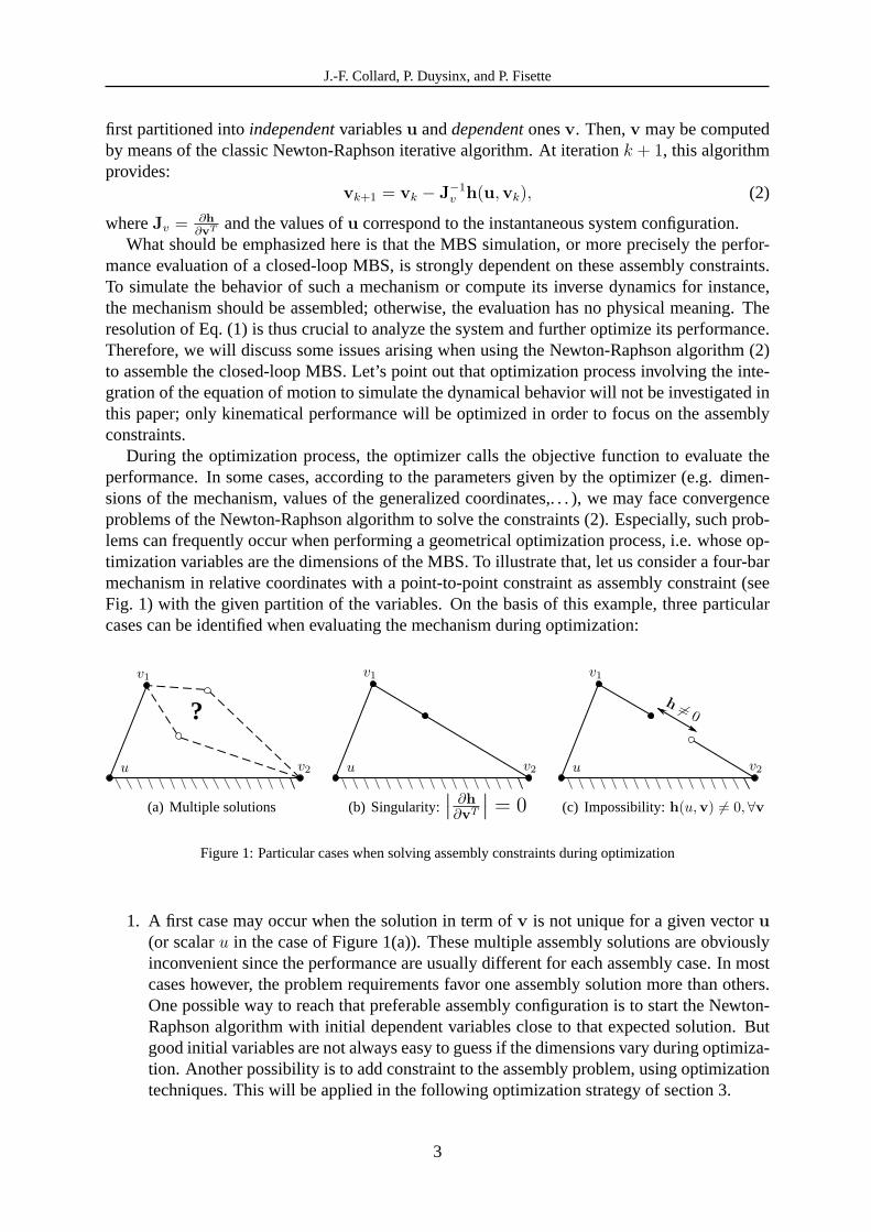
During the optimization process, the optimizer calls the objective function to evaluate theperformance. In some cases, according to the parameters given by the optimizer (e.g. dimen-sions of the mechanism, values of the generalized coordinates,. . . ), we may face convergenceproblems of the Newton-Raphson algorithm to solve the constraints (2). Especially, such prob-lems can frequently occur when performing a geometrical optimization process, i.e. whose op-timization variables are the dimensions of the MBS. To illustrate that, let us consider a four-barmechanism in relative coordinates with a point-to-point constraint as assembly constraint (seeFig. 1) with the given partition of the variables. On the basis of this example, three particularcases can be identified when evaluating the mechanism duringoptimization:
u
v1
v2
?
(a) Multiple solutions
u
v1
v2
(b) Singularity:∣
∣
∂h∂vT
∣
∣ = 0
u
v1
v2
h 6= 0
(c) Impossibility:h(u,v) 6= 0,∀v
Figure 1: Particular cases when solving assembly constraints during optimization
1. A first case may occur when the solution in term ofv is not unique for a given vectoru(or scalaru in the case of Figure 1(a)). These multiple assembly solutions are obviouslyinconvenient since the performance are usually different for each assembly case. In mostcases however, the problem requirements favor one assemblysolution more than others.One possible way to reach that preferable assembly configuration is to start the Newton-Raphson algorithm with initial dependent variables close tothat expected solution. Butgood initial variables are not always easy to guess if the dimensions vary during optimiza-tion. Another possibility is to add constraint to the assembly problem, using optimizationtechniques. This will be applied in the following optimization strategy of section 3.
3
J.-F. Collard, P. Duysinx, and P. Fisette
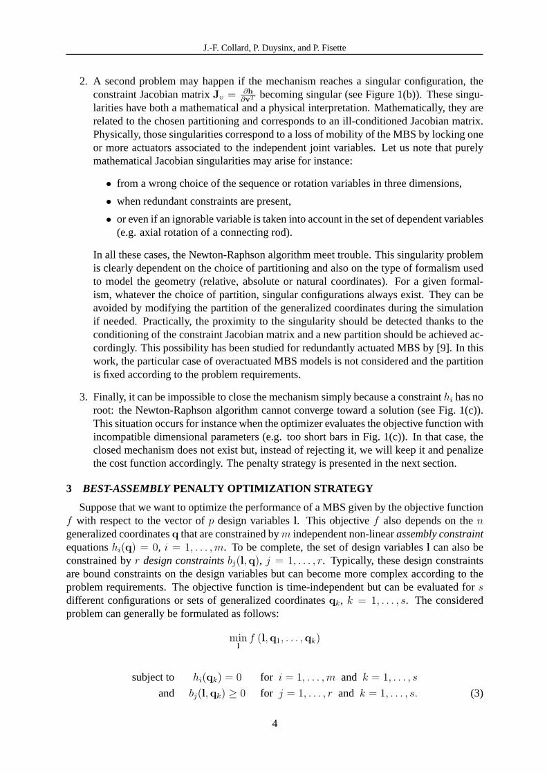
2. A second problem may happen if the mechanism reaches a singular configuration, theconstraint Jacobian matrixJv = ∂h
∂vT becoming singular (see Figure 1(b)). These singu-larities have both a mathematical and a physical interpretation. Mathematically, they arerelated to the chosen partitioning and corresponds to an ill-conditioned Jacobian matrix.Physically, those singularities correspond to a loss of mobility of the MBS by locking oneor more actuators associated to the independent joint variables. Let us note that purelymathematical Jacobian singularities may arise for instance:
• from a wrong choice of the sequence or rotation variables in three dimensions,
• when redundant constraints are present,
• or even if an ignorable variable is taken into account in the set of dependent variables(e.g. axial rotation of a connecting rod).
In all these cases, the Newton-Raphson algorithm meet trouble. This singularity problemis clearly dependent on the choice of partitioning and also on the type of formalism usedto model the geometry (relative, absolute or natural coordinates). For a given formal-ism, whatever the choice of partition, singular configurations always exist. They can beavoided by modifying the partition of the generalized coordinates during the simulationif needed. Practically, the proximity to the singularity should be detected thanks to theconditioning of the constraint Jacobian matrix and a new partition should be achieved ac-cordingly. This possibility has been studied for redundantly actuated MBS by [9]. In thiswork, the particular case of overactuated MBS models is not considered and the partitionis fixed according to the problem requirements.
3. Finally, it can be impossible to close the mechanism simply because a constrainthi has noroot: the Newton-Raphson algorithm cannot converge toward asolution (see Fig. 1(c)).This situation occurs for instance when the optimizer evaluates the objective function withincompatible dimensional parameters (e.g. too short bars in Fig. 1(c)). In that case, theclosed mechanism does not exist but, instead of rejecting it, we will keep it and penalizethe cost function accordingly. The penalty strategy is presented in the next section.
3 BEST-ASSEMBLY PENALTY OPTIMIZATION STRATEGY
Suppose that we want to optimize the performance of a MBS givenby the objective functionf with respect to the vector ofp design variablesl. This objectivef also depends on thengeneralized coordinatesq that are constrained bym independent non-linearassembly constraintequationshi(q) = 0, i = 1, . . . ,m. To be complete, the set of design variablesl can also beconstrained byr design constraintsbj(l,q), j = 1, . . . , r. Typically, these design constraintsare bound constraints on the design variables but can becomemore complex according to theproblem requirements. The objective function is time-independent but can be evaluated forsdifferent configurations or sets of generalized coordinates qk, k = 1, . . . , s. The consideredproblem can generally be formulated as follows:
minl
f (l,q1, . . . ,qk)
subject to hi(qk) = 0 for i = 1, . . . ,m and k = 1, . . . , s
and bj(l,qk) ≥ 0 for j = 1, . . . , r and k = 1, . . . , s. (3)
4
J.-F. Collard, P. Duysinx, and P. Fisette
The proposed strategy to solve (3) is an alternative of the artificial penalty strategy devel-oped in Ref. [5]. It is based on the minimization of the assembly constraints instead of theirresolution. This is the main difference which will imply thepossible use of gradient-basedoptimization methods such as quasi-Newton methods or the sequential quadratic programming(SQP) technique. The key idea of the method is developed in the following.
Practically, after the partitioning of the generalized coordinates, the resolution of the con-straint equations (1) is replaced by the following constrained optimization problem:
minv
1
2h(l,u,v)Th(l,u,v)
subject toc(l,u,v) ≥ 0. (4)
This replacement can be seen as an extension of the assembly problem. Indeed, if the as-sembly constraints can be satisfied, solution of problem (4)reaches a zero value as with theNewton-Raphson resolution. Otherwise, the square norm of the assembly constraint vectorh
is minimized while the Newton-Raphson algorithm would not have provided a consistent resultto the assembly problem. This new formulation offers a direct solution to the assembly issue3 described in section 2, for which the dimensions of the mechanism are not compatible withassembly constraints.
Now, if we consider assembly issues due to multiple solutions and singular configurations(issues 1 and 2 in section 2), formulation (4) can also help usto avoid these problems, using theadditional optimization inequality constraintc ∈ <mc . If functionc is well chosen, the assemblyproblem can be restricted to a regular and unique solution. The definition of this additionalconstraint therefore requires to know in advance the different solutions and singularities of theassembly problem. This prerequisite can sometimes be difficult to establish when complextopologies are considered. However, for many applicationsinvolving several simple loops ofbodies such as parallel manipulators (see applications in section 5), the build of functioncremains affordable.
θ1
θ2
θ3
I1
I2
A
B
l1
l2
l3
l4
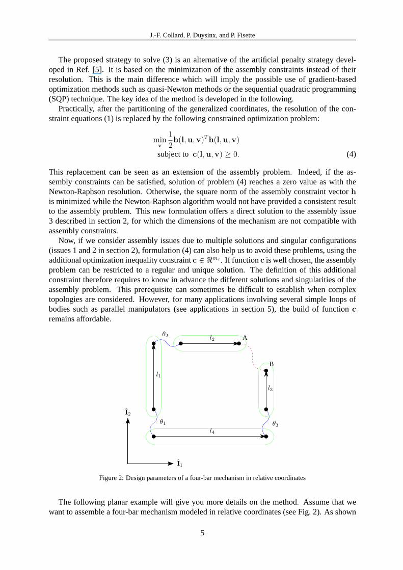
Figure 2: Design parameters of a four-bar mechanism in relative coordinates
The following planar example will give you more details on the method. Assume that wewant to assemble a four-bar mechanism modeled in relative coordinates (see Fig. 2). As shown
5
J.-F. Collard, P. Duysinx, and P. Fisette
in Fig.1(a), two assembly solutions exist. The additional requirement is to keep the “elbow-up”closed configuration (i.e. when pointsA orB remain above the straight line betweenθ2 andθ3
in Fig. 2) and to avoid the singular configurations when bars are aligned. This model contains3 generalized coordinatesθ1,θ2, andθ3. The four bars have lengthsl1, l2, l3 andl4. To makepointsA andB coincide, the two assembly equations are:
h1(θ1, θ2, θ3) = −l1 sin θ1 + l2 cos (θ1 + θ2) + l3 sin θ3 − l4 = 0, (5)
h2(θ1, θ2, θ3) = l1 cos θ1 + l2 sin (θ1 + θ2) − l3 cos θ3 = 0. (6)
To solve the initial position problem orassembly problem, solution of the non-linear sys-tem (5) – (6) has to be found. This implies thepartitioning of the three variablesθ1, θ2 andθ3 into one independent variableu and two dependent onesv. Assume this partition is chosenas:u = θ1, v = [θ2 θ3]
T . To detect singular configurations, we compute the determinant ofJv
as:|Jv| = cos (θ1 + θ2 − θ3) . (7)
This determinant vanishes at the singularity and its signs defines two regions of the joint spacecorresponding to the “elbow-up” and “elbow-down” configurations. Tosafelychoose the “elbow-up” configuration during assembly process, the additional inequality constraintc ≥ 0 will be:
c (θ1, θ2, θ3) = cos (θ1 + θ2 − θ3) − cth ≥ 0, (8)
wherecth is a positive threshold constant that define a safety gap fromthe singularity. The valueof cth (typically cth = 0.01) will keep the assembly process far from the singularity even if themechanism cannot be assembled. This will ensure a regular consistent optimal solution to thedesign optimization problem (3).
G XB
g(X)g
f
fpen = minv
1
2h
Th
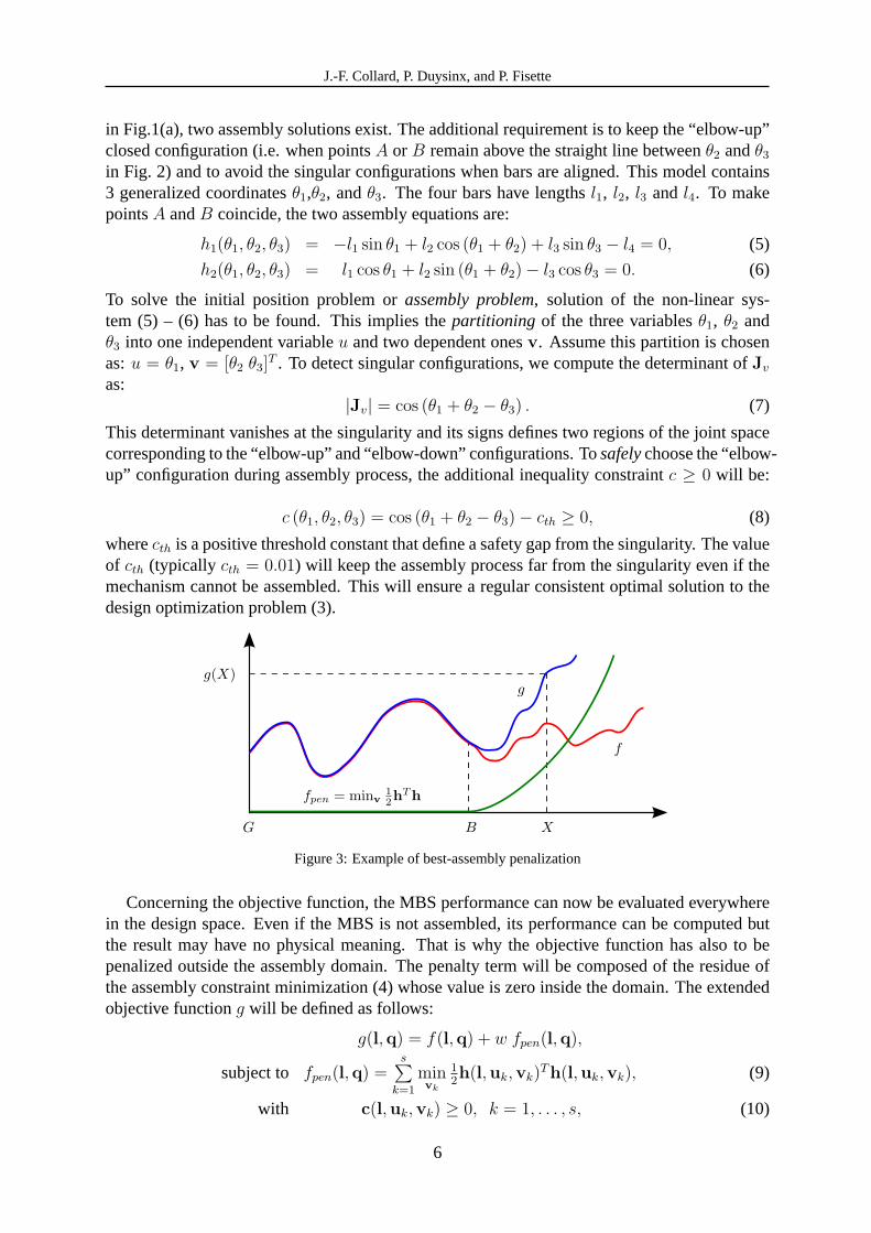
Figure 3: Example of best-assembly penalization
Concerning the objective function, the MBS performance can now be evaluated everywherein the design space. Even if the MBS is not assembled, its performance can be computed butthe result may have no physical meaning. That is why the objective function has also to bepenalized outside the assembly domain. The penalty term will be composed of the residue ofthe assembly constraint minimization (4) whose value is zero inside the domain. The extendedobjective functiong will be defined as follows:
g(l,q) = f(l,q) + w fpen(l,q),
subject to fpen(l,q) =s
∑
k=1
minvk
1
2h(l,uk,vk)
Th(l,uk,vk), (9)
with c(l,uk,vk) ≥ 0, k = 1, . . . , s, (10)
6
J.-F. Collard, P. Duysinx, and P. Fisette
wherew is a weighted factor between the actual performancef and the penalty termfpen. Thisdefinition is illustrated in one dimension in Fig. 3. The mainadvantage of this new formulationis thatg is always continuous and always differentiable over the design space. This propertyenables us to use gradient-based algorithms that are local methods but often more efficient thandirect searches or stochastic algorithms.
?
Computation ofbl(l)
?
minv1
2h(l,u,v)th(l,u,v)
such thatc(l,u,v) ≥ 0
?
Performance evaluation
?
Computation ofblq(l,q)
?
Sensitivity Analysis
?
������
PPPPPP
������
PPPPPPOther
config. ?y
n
6
Optimizer
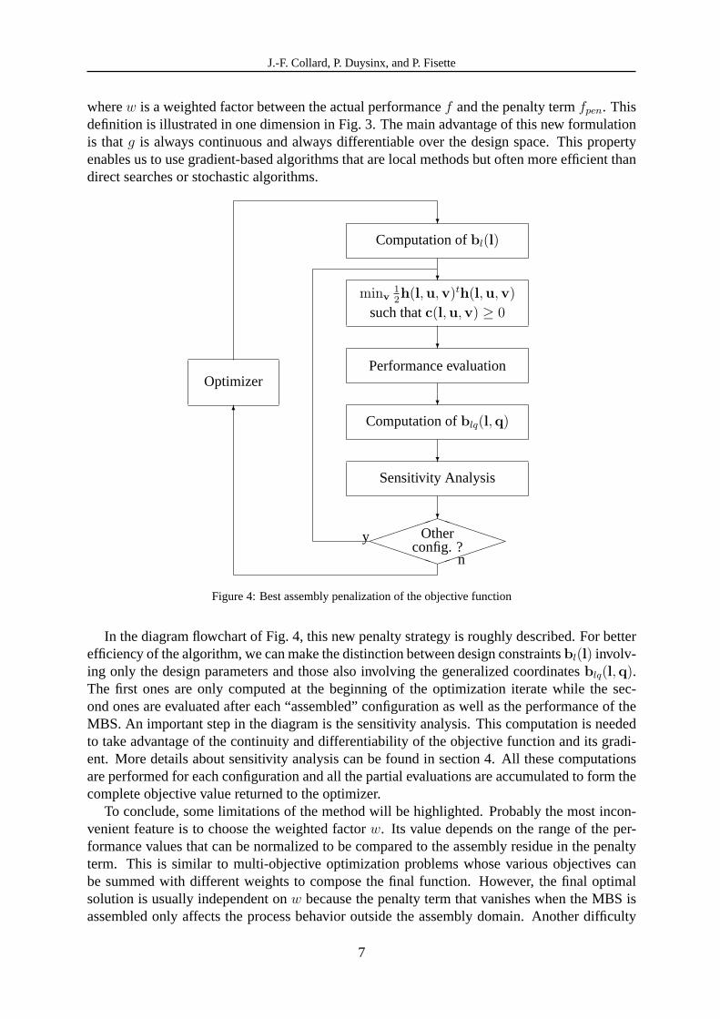
Figure 4: Best assembly penalization of the objective function
In the diagram flowchart of Fig. 4, this new penalty strategy is roughly described. For betterefficiency of the algorithm, we can make the distinction between design constraintsbl(l) involv-ing only the design parameters and those also involving the generalized coordinatesblq(l,q).The first ones are only computed at the beginning of the optimization iterate while the sec-ond ones are evaluated after each “assembled” configurationas well as the performance of theMBS. An important step in the diagram is the sensitivity analysis. This computation is neededto take advantage of the continuity and differentiability of the objective function and its gradi-ent. More details about sensitivity analysis can be found insection 4. All these computationsare performed for each configuration and all the partial evaluations are accumulated to form thecomplete objective value returned to the optimizer.
To conclude, some limitations of the method will be highlighted. Probably the most incon-venient feature is to choose the weighted factorw. Its value depends on the range of the per-formance values that can be normalized to be compared to the assembly residue in the penaltyterm. This is similar to multi-objective optimization problems whose various objectives canbe summed with different weights to compose the final function. However, the final optimalsolution is usually independent onw because the penalty term that vanishes when the MBS isassembled only affects the process behavior outside the assembly domain. Another difficulty
7
J.-F. Collard, P. Duysinx, and P. Fisette
could be to find the additional constraintc and the choice ofcth (e.g. in Eq. (8)). This parameterinfluences the safety with respect to singularity. However,it is possible to give a geometricalmeaning to the constantcth.
4 SENSITIVITY ANALYSIS
Before using gradient-based optimization techniques, it isnecessary to analyze the sensitivityof the penalized objective functiong (Eq. (10)) with respect to the vector of design parametersl. To alleviate the notation, let us consider only one set of generalized coordinatesq. We candefine the reduced objective functiong∗ for which the assembly problem (4) is solved:
g∗ (l,u) ≡ g (l,u,v∗(u, l)) , (11)
where the independent variablesu are constant for the optimization problem andv∗ is thesolution of problem (4).
When the optimal assembly solution is found, the Kuhn-Tuckerfirst-order necessary condi-tion of this constrained optimization problem can be applied. This means that the LagrangianL of the constrained problem (4) is vanishes at the optimal solution. Practically,L is defined inour case as follows:
L(l,u,v,λ) =1
2h(l,u,v)Th(l,u,v) − λ
Tc(l,u,v), (12)
whereλ ∈ <mc is the vector of Lagrangian multipliers. These multiplierscan be considered asadditional dependent variables of the assembly problem. Wetherefore define an extended setv
of dependent variables:
v ≡
[
v
λ
]
. (13)
According to the Kuhn-Tucker theorem [13], we can write the following necessary conditions:
∂L
∂vT(l,u,v∗,λ∗) = 0, (14)
λ∗i ≥ 0, i = 1, . . . ,mc, (15)
λ∗i ci(l,u,v∗) = 0, i = 1, . . . ,mc, (16)
where the asterisk symbol refers to a local constrained minimizer of problem (4). Note thatthese conditions assume that the gradients∂c
∂vT of all active constraints are linearly independent.The new extended functionh is then defined as:
h(l,u, v) ≡
[
∂L∂v
(l,u,v,λ)diag(λ) c(l,u,v)
]
, (17)
where diag(λ) is a square matrix containing the elements of vectorλ on its diagonal. Thisextended functionh reaches a zero value when the best-assembly problem (4) is solved.
For further developments, the Jacobian matrix ofh with respect to the design variables isgiven by:
∂h
∂lT=
[
∂2L∂lT ∂v
diag(λ) ∂c
∂lT
]
=
m∑
i=1
∂2hi
∂lT ∂vhi + ∂h
T
∂v
∂h
∂lT−
mc∑
i=1
λi∂2ci
∂lT ∂v
diag(λ) ∂c
∂lT
, (18)
8
J.-F. Collard, P. Duysinx, and P. Fisette
and the Jacobian matrix ofh with respect to the extended dependent variables is:
∂h
∂vT=
[
∂h
∂vT∂h
∂λT
]
=
[
∂2L∂vT ∂v
∂2L
∂λT ∂v
diag(λ) ∂c
∂vT diag(c)
]
=
m∑
i=1
∂2hi
∂vT ∂vhi + ∂h
T
∂v
∂h
∂vT −mc∑
i=1
λi∂2ci
∂vT ∂v−∂c
T
∂v
diag(λ) ∂c
∂vT diag(c)
, (19)
where diag(c) is a square matrix containing the elements of vectorc on its diagonal.In the following, two well-known techniques are presented to calculate the derivatives of
objective functiong subject to the constraintsh = 0 .
4.1 Direct Method
The first method coming in mind to analyze the sensitivity ofg is called thedirect method.Using the chain rule applied to functiong∗, we obtain:
∂g∗
∂lT=
∂g
∂lT+
∂g
∂vT
∂v∗
∂lT. (20)
The remaining unknows are the partial derivatives ofv∗ with respect to the design parameters.These can be found by differentiating them+mc equations of constraintsh(l,u, v∗(u, l)) = 0.This gives us:
∂h
∂lT+
∂h
∂vT
∂v∗
∂lT= 0, (21)
from which we can easily derived:
∂v∗
∂lT= −
(
∂h
∂vT
)−1∂h
∂lT, (22)
if the Jacobian matrixJv = ∂h
∂vT is invertible. Note thatJv is always a square matrix since theremust be as many constraint equations as dependent variables.
In conclusion, ifJv is regular, Eq. (22) can be inserted in Eq. (20) to yield the sensitivity ofg∗ with respect to the design variables:
∂g∗
∂lT=
∂g
∂lT−
∂g
∂vT
(
∂h
∂vT
)−1∂h
∂lT. (23)
4.2 Adjoint Method
Another well-known method to derive the sensitivity of the objective functiong is to use theadjoint method. This method is considered as the dual of the direct method. The basic idea isto artificially adjoin a linear combination of the constraint equations to the objective function.As these constraint equations are assumed to be satisfied or identically equal to zero, this doesnot modify the value ofg∗. We can thus defineg∗:
g∗ (l,u) ≡ g∗ (l,u) + νT h(l,u, v∗(u, l)) = g∗ (l,u) , ∀ν ∈ <m. (24)
9
J.-F. Collard, P. Duysinx, and P. Fisette
This extended objective functiong∗ can then be derived with respect to the design parameters.This provides us with:
∂g∗
∂lT=
∂g
∂lT+
∂g
∂vT
∂v∗
∂lT+ ν
T
(
∂h
∂lT+
∂h
∂vT
∂v∗
∂lT
)
=∂g
∂lT+ ν
T ∂h
∂lT+
(
∂g
∂vT+ ν
T ∂h
∂vT
)
∂v∗
∂lT. (25)
Now, the trick to avoid the computation of∂v∗
∂lTis to choose the adjoint variablesν such that:
∂g
∂vT+ ν
T ∂h
∂vT= 0
⇔∂g
∂v+∂hT
∂vν = 0
⇔ ν = −
(
∂hT
∂v
)−1∂g
∂v. (26)
This last line is consistent if∂hT
∂vis regular, i.e. ifJv is invertible since∂h
T
∂v= (Jv)
T .Finally, after the insertion of Eq. (26) into Eq. (25), we obtain:
∂g∗
∂lT=
∂g
∂lT−
∂g
∂vT
(
∂h
∂vT
)−1∂h
∂lT, (27)
which is strictly equivalent to Eq. (23). This remark is obvious in our case because the numberof independent constraintsh is the same as the number of dependent variablesv.
5 APPLICATIONS: KINETOSTATIC OPTIMIZATION OF PARALLEL ROBOTS
Isotropyof a manipulator is a kinetostatic performance that can be measured from the condi-tion numberκ of its forward kinematics Jacobian matrixJf [2]. In other words, if this JacobianJf is defined by:
x = Jf qa (28)
whereqa is the velocity vector of the actuated joints andx the end-effector twist defined by theCartesian (position) and angular (orientation) velocity vectors of the end-effector, this isotropyindexκ is the condition number ofJf [2]. It can be written as the ratio of the largest singularvalueσl of Jf to its smallest oneσs:
κ (Jf ) =σl
σs
. (29)
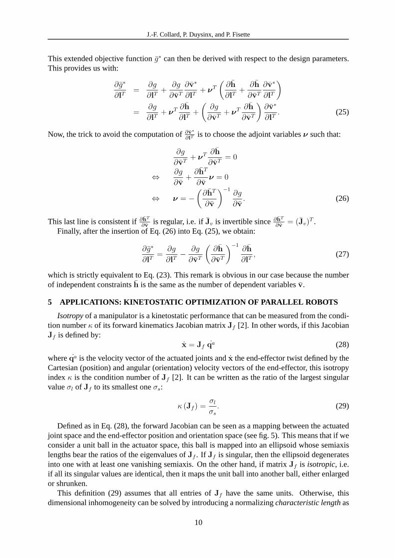
Defined as in Eq. (28), the forward Jacobian can be seen as a mapping between the actuatedjoint space and the end-effector position and orientation space (see fig. 5). This means that if weconsider a unit ball in the actuator space, this ball is mapped into an ellipsoid whose semiaxislengths bear the ratios of the eigenvalues ofJf . If Jf is singular, then the ellipsoid degeneratesinto one with at least one vanishing semiaxis. On the other hand, if matrixJf is isotropic, i.e.if all its singular values are identical, then it maps the unit ball into another ball, either enlargedor shrunken.
This definition (29) assumes that all entries ofJf have the same units. Otherwise, thisdimensional inhomogeneity can be solved by introducing a normalizingcharacteristic lengthas
10
J.-F. Collard, P. Duysinx, and P. Fisette
qa1
qa2
qa3
x1
x2
x3Jf
Figure 5: Jacobian mapping between actuated coordinatesqi and tool coordinatesxi
suggested in [2]. The latter is used to divide the positioning rows ofJf , making it dimensionallyhomogeneous. As explained in [2], let us note that the value of the characteristic length itselfcomes from the minimization of the condition number over allthe reachable configurations.
In the following applications, the goal is to optimize a global posture-independent perfor-mance index which is the mean of the inverses of the conditionnumberκ over a volumeV inthe Cartesian space of the end-effector, also called Global Dexterity Index (GDI) [8]:
GDI =
∫
V
1
κdV
V(30)
In the case of positioning and orientating manipulators (for instance, the Hunt platform de-scribed in section 5.2), the value ofκ is obviously computed after normalizing the Jacobianmatrix, as previously explained. By analogy with the optimization proposed in [2], we suggestthat the above-mentioned characteristic length becomes anadditional parameter of our opti-mization problem which initially only deals with purely design parameters.
The optimization of this global dexterity index (30) will befirst performed on the Deltaparallel robot, whose moving platform has only 3 translational dof. In the second subsection, amore complex model will be considered where the moving platform has 6 dof (3 positions and3 orientations): the Hunt platform.
5.1 Optimization of the translational Delta Robot
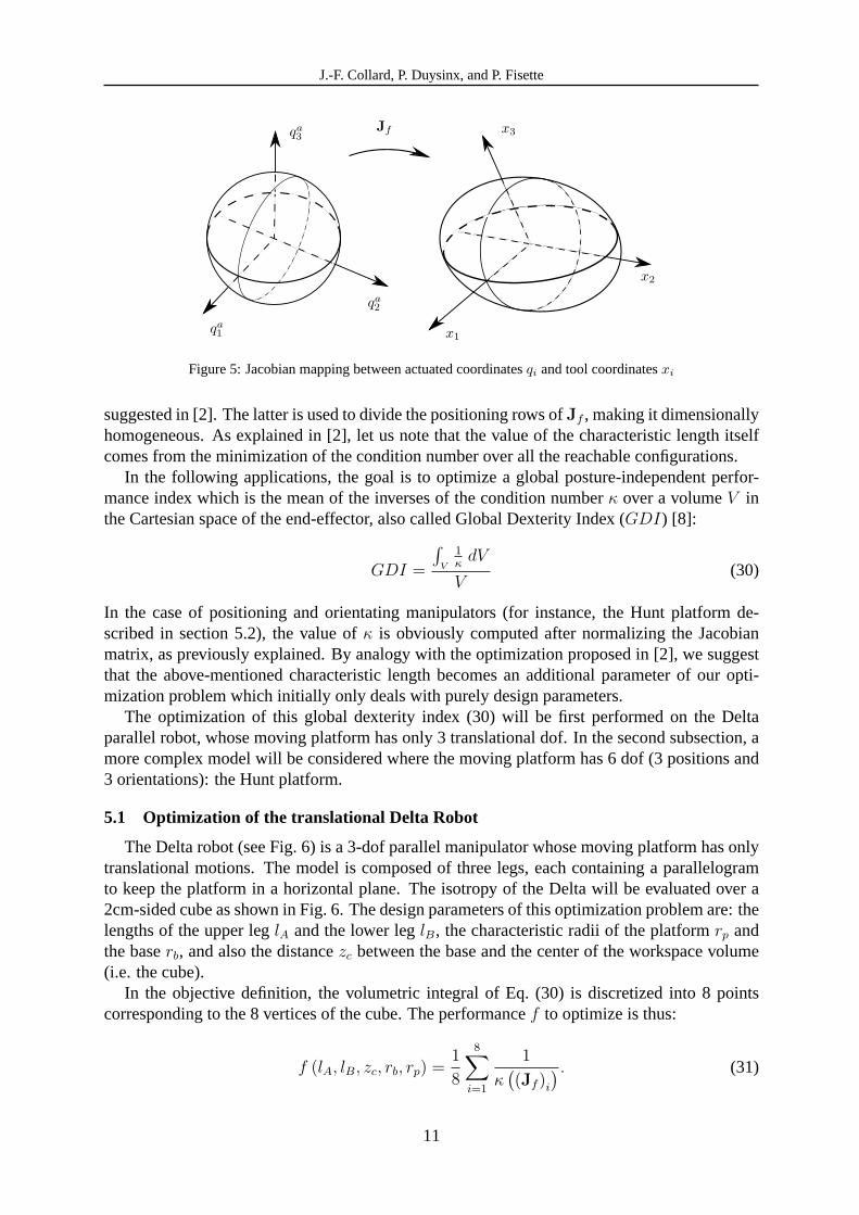
The Delta robot (see Fig. 6) is a 3-dof parallel manipulator whose moving platform has onlytranslational motions. The model is composed of three legs,each containing a parallelogramto keep the platform in a horizontal plane. The isotropy of the Delta will be evaluated over a2cm-sided cube as shown in Fig. 6. The design parameters of this optimization problem are: thelengths of the upper leglA and the lower leglB, the characteristic radii of the platformrp andthe baserb, and also the distancezc between the base and the center of the workspace volume(i.e. the cube).
In the objective definition, the volumetric integral of Eq. (30) is discretized into 8 pointscorresponding to the 8 vertices of the cube. The performancef to optimize is thus:
f (lA, lB, zc, rb, rp) =1
8
8∑
i=1
1
κ(
(Jf )i
) . (31)
11
J.-F. Collard, P. Duysinx, and P. Fisette
lA
lB
zc
rb
rp
Figure 6: Delta robot model
The computation ofJf is obtained from the derivation of the constraint equationshi = 0which involve the joint coordinates of the 3 actuatorsqa = (qa
1 , qa2 , q
a3) between the base and
the leg as well as the Cartesian coordinatesx = (x, y, z) of the moving platform. Note thatthis computation is only valid inside the assembly domain whereh = 0. Practically, afterthe coordinate partitioning, the derivation ofh yields the relation between independent anddependent velocity vectors:
v = Bvuu, (32)
whereBvu , − (Jv)−1
Ju is the coupling matrix. In our case, the independent variables corre-sponds to the platform coordinates (u = x) while the actuated variables belongs to the depen-dent variable set. A second partition of the dependent variables gives:
v =
[
qa
qf
]
, (33)
whereqf is the vector of the free (non actuated) dependent variables. Accordingly, relation (32)becomes:
[
qa
qf
]
=
[
Bqau
Bqf u
]
x, (34)
from which we can deduce in comparison with Eq. (28) that:
Jf = B−1
qau. (35)
Therefore, in Eq. (31), the condition number ofJf is equal to the condition number ofBqau.This optimization problem has also some restrictions to satisfy. Bound constraints have been
specified to get a reasonable solution. Minimum and maximum values are reported in Table 2.Concerning the assembly problem, we should avoid to close themechanism toward an “inside”position of the legs as shown in Fig. 7. Therefore, some inequality constraintsc have beenformulated in terms of sines and cosines of the dependent variables. All these considerationslead to the extended objective functiong (see Eq. 10).
The optimization has been first performed with only 2 of the 5 parameters to visualize theprocess. The leg lengths are optimized but the radiirp andrb, and the distancezc are fixed:rp = 2cm, rb = 5cm, andzc = −10cm. Two different starting pointsStart1 andStart2 areproposed to highlight the existence of two different local minima. The optimization processcan be observed in Fig. 8. The constrained optimization algorithm is the well-known sequentialquadratic programming method (SQP) [13]. From both starting points, the process converges
12
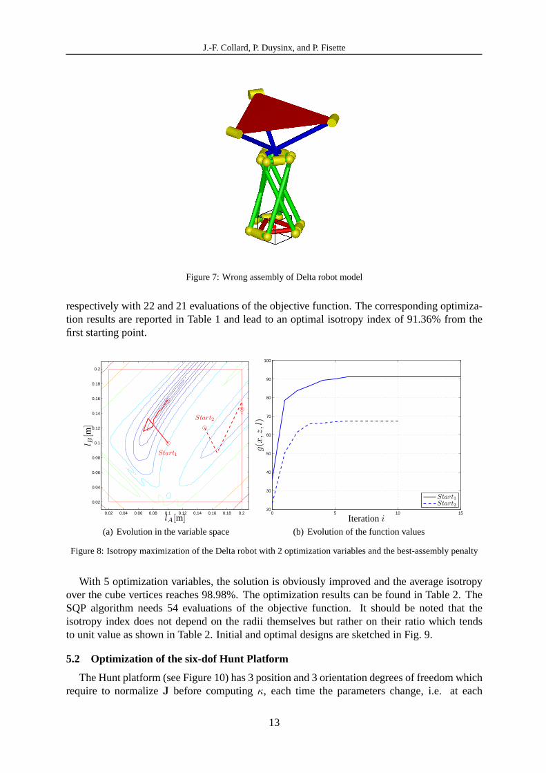
J.-F. Collard, P. Duysinx, and P. Fisette
Figure 7: Wrong assembly of Delta robot model
respectively with 22 and 21 evaluations of the objective function. The corresponding optimiza-tion results are reported in Table 1 and lead to an optimal isotropy index of 91.36% from thefirst starting point.
Start1
Start2
0.02 0.04 0.06 0.08 0.1 0.12 0.14 0.16 0.18 0.2
0.02
0.04
0.06
0.08
0.1
0.12
0.14
0.16
0.18
0.2
lA[m]
l B[m
]
(a) Evolution in the variable space
0 5 10 1520
30
40
50
60
70
80
90
100
Start1Start2
g(x,z,l
)
Iterationi
(b) Evolution of the function values
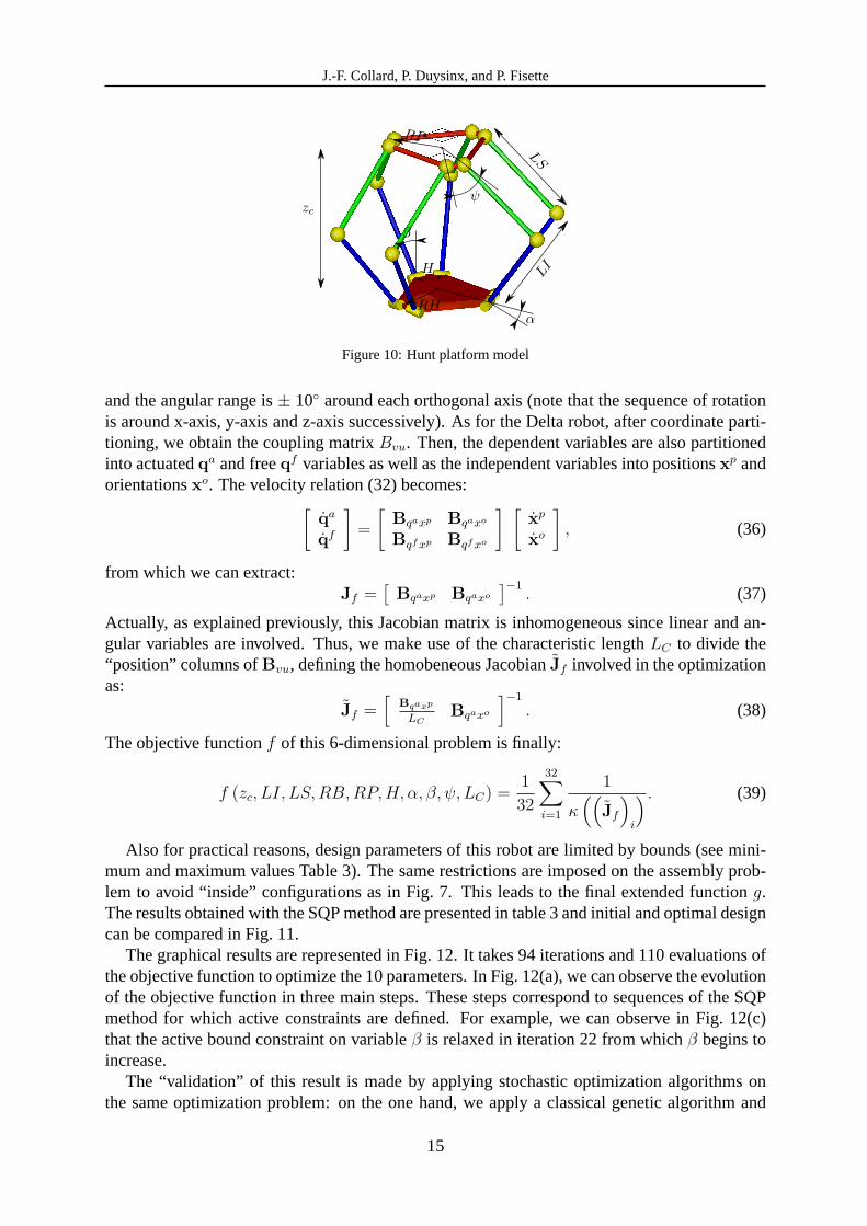
Figure 8: Isotropy maximization of the Delta robot with 2 optimization variables and the best-assembly penalty
With 5 optimization variables, the solution is obviously improved and the average isotropyover the cube vertices reaches 98.98%. The optimization results can be found in Table 2. TheSQP algorithm needs 54 evaluations of the objective function. It should be noted that theisotropy index does not depend on the radii themselves but rather on their ratio which tendsto unit value as shown in Table 2. Initial and optimal designsare sketched in Fig. 9.
5.2 Optimization of the six-dof Hunt Platform
The Hunt platform (see Figure 10) has 3 position and 3 orientation degrees of freedom whichrequire to normalizeJ before computingκ, each time the parameters change, i.e. at each
13

J.-F. Collard, P. Duysinx, and P. Fisette
Start1 Start2
GDIopt [%] 91.36 67.64la,opt [cm] 9.91 20.00lb,opt [cm] 15.66 14.57GDI0 [%] 36.11 23.16la,0 [cm] 10.00 15.00lb,0 [cm] 10.00 12.00
Table 1: Isotropy maximization of the Delta robot with 2 optimization variables
Minimum Initial Maximum Optimal
GDI [%] 36.11 98.88la [cm] 2.00 10.00 20.00 16.39lb [cm] 2.00 10.00 20.00 20.00z [cm] -20.00 -10.00 -5.00 -11.53rb [cm] 1.00 5.00 10.00 6.02rp [cm] 1.00 2.00 10.00 6.05
Table 2: Isotropy maximization of the Delta robot with 5 optimization variables
call of the objective function. As explained above, this involves an additional optimizationparameter: the characteristic lengthLC . The nine other parameters of this optimization problem(see Fig. 10) are the legs lengthsLI andLS, the characteristic radius of the platformRP andof the baseRB, the gaugeH between adjoining actuators on the base, the angleα (around avertical axis), followed by angleβ (around an horizontal axis), angleψ, and finally the verticaldistancezc between the base and the center of the desired workspace volume (small cube inFig. 10).
The objective function is similar to (31) for the Delta robotexcept that now the forwardJacobian matrixJf has 6 rows for the 3 positions and the 3 orientations of the platform and6 columns for the 6 actuated joint variables between the baseand the 6 legs. Therefore, theaverage value of isotropy has to be computed over a 6-dimension hyper-cube, or more preciselyover its 32 vertices. According to the research project specifications (for a surgical application),this cube has a side length of 50 mm (i.e.± 25 mm from the center point) in the Cartesian space
(a) Initial design (b) Optimal design
Figure 9: Optimal designs for the isotropy maximization of the Delta robot
14
J.-F. Collard, P. Duysinx, and P. Fisette
zc
LI
LS
RB
RP
H
α
β
ψ
Figure 10: Hunt platform model
and the angular range is± 10◦ around each orthogonal axis (note that the sequence of rotationis around x-axis, y-axis and z-axis successively). As for the Delta robot, after coordinate parti-tioning, we obtain the coupling matrixBvu. Then, the dependent variables are also partitionedinto actuatedqa and freeqf variables as well as the independent variables into positionsxp andorientationsxo. The velocity relation (32) becomes:
[
qa
qf
]
=
[
Bqaxp Bqaxo
Bqf xp Bqf xo
] [
xp
xo
]
, (36)
from which we can extract:Jf =
[
Bqaxp Bqaxo
]−1. (37)
Actually, as explained previously, this Jacobian matrix isinhomogeneous since linear and an-gular variables are involved. Thus, we make use of the characteristic lengthLC to divide the“position” columns ofBvu, defining the homobeneous JacobianJf involved in the optimizationas:
Jf =[
Bqaxp
LCBqaxo
]−1
. (38)
The objective functionf of this 6-dimensional problem is finally:
f (zc, LI, LS,RB,RP,H, α, β, ψ, LC) =1
32
32∑
i=1
1
κ((
Jf
)
i
) . (39)
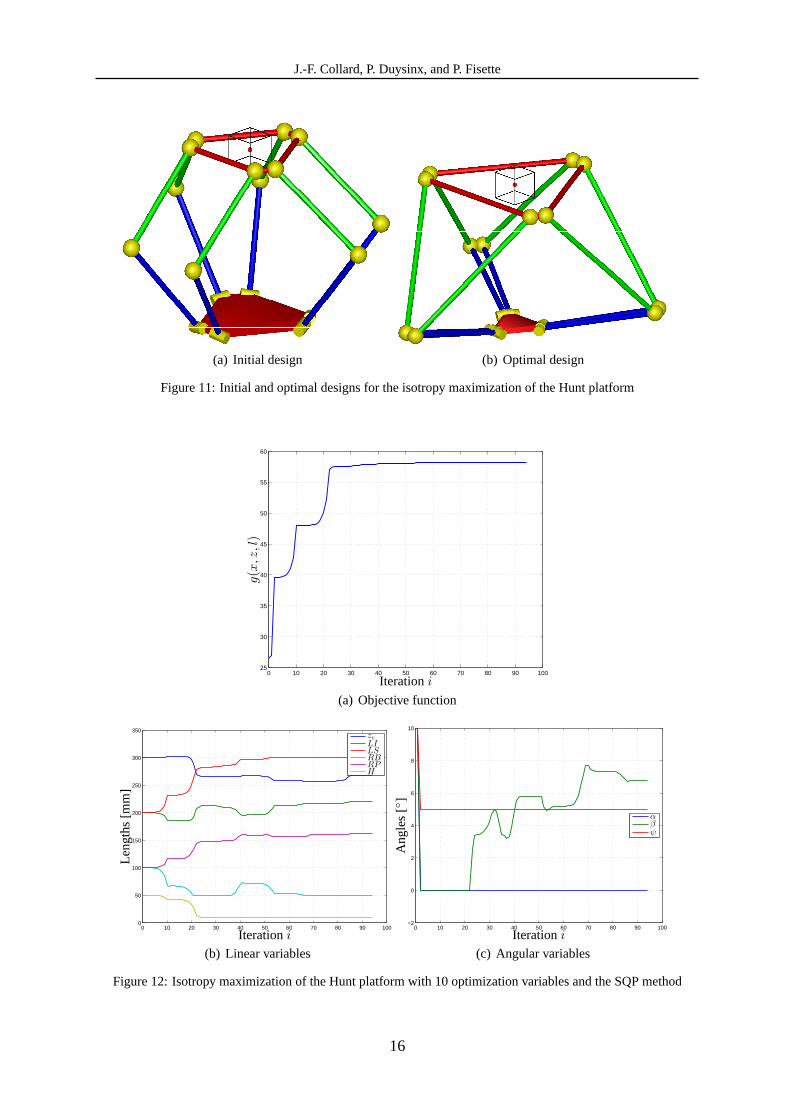
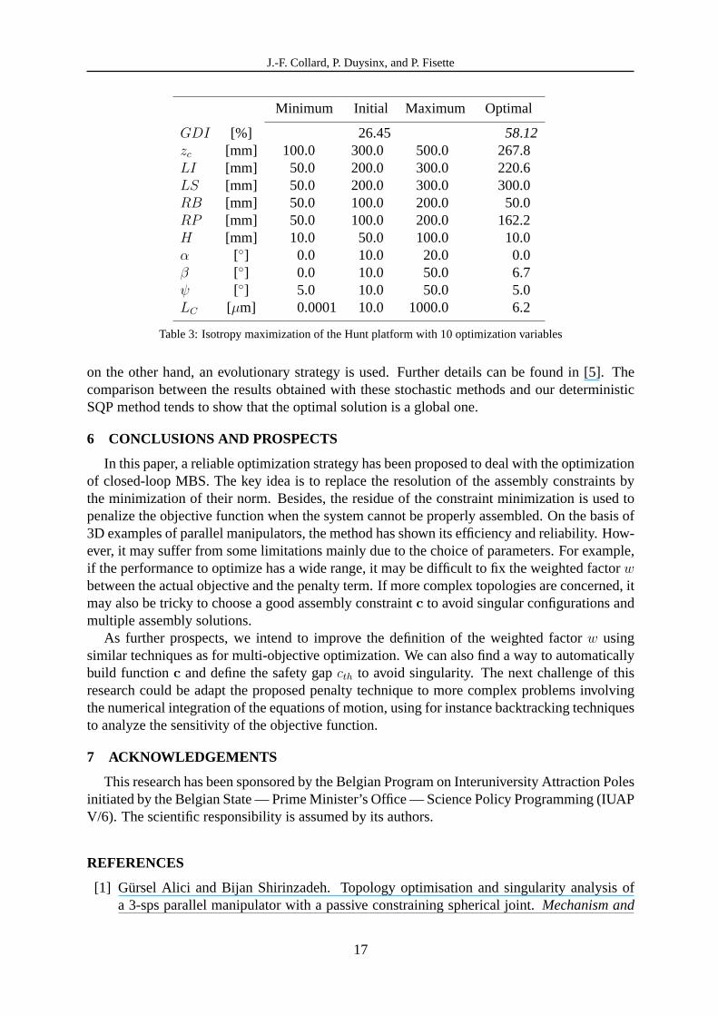
Also for practical reasons, design parameters of this robotare limited by bounds (see mini-mum and maximum values Table 3). The same restrictions are imposed on the assembly prob-lem to avoid “inside” configurations as in Fig. 7. This leads to the final extended functiong.The results obtained with the SQP method are presented in table 3 and initial and optimal designcan be compared in Fig. 11.
The graphical results are represented in Fig. 12. It takes 94iterations and 110 evaluations ofthe objective function to optimize the 10 parameters. In Fig. 12(a), we can observe the evolutionof the objective function in three main steps. These steps correspond to sequences of the SQPmethod for which active constraints are defined. For example, we can observe in Fig. 12(c)that the active bound constraint on variableβ is relaxed in iteration 22 from whichβ begins toincrease.
The “validation” of this result is made by applying stochastic optimization algorithms onthe same optimization problem: on the one hand, we apply a classical genetic algorithm and
15
J.-F. Collard, P. Duysinx, and P. Fisette
(a) Initial design (b) Optimal design
Figure 11: Initial and optimal designs for the isotropy maximization of the Hunt platform
0 10 20 30 40 50 60 70 80 90 10025
30
35
40
45
50
55
60
Iterationi
g(x,z,l
)
(a) Objective function
0 10 20 30 40 50 60 70 80 90 1000
50
100
150
200
250
300
350
zc
LILSRBRPH
Iterationi
Leng
ths
[mm
]
(b) Linear variables
0 10 20 30 40 50 60 70 80 90 100−2
0
2
4
6
8
10
αβψ
Iterationi
Ang
les
[◦]
(c) Angular variables
Figure 12: Isotropy maximization of the Hunt platform with 10 optimization variables and the SQP method
16
J.-F. Collard, P. Duysinx, and P. Fisette
Minimum Initial Maximum Optimal
GDI [%] 26.45 58.12zc [mm] 100.0 300.0 500.0 267.8LI [mm] 50.0 200.0 300.0 220.6LS [mm] 50.0 200.0 300.0 300.0RB [mm] 50.0 100.0 200.0 50.0RP [mm] 50.0 100.0 200.0 162.2H [mm] 10.0 50.0 100.0 10.0α [◦] 0.0 10.0 20.0 0.0β [◦] 0.0 10.0 50.0 6.7ψ [◦] 5.0 10.0 50.0 5.0LC [µm] 0.0001 10.0 1000.0 6.2
Table 3: Isotropy maximization of the Hunt platform with 10 optimization variables
on the other hand, an evolutionary strategy is used. Furtherdetails can be found in [5]. Thecomparison between the results obtained with these stochastic methods and our deterministicSQP method tends to show that the optimal solution is a globalone.
6 CONCLUSIONS AND PROSPECTS
In this paper, a reliable optimization strategy has been proposed to deal with the optimizationof closed-loop MBS. The key idea is to replace the resolution of the assembly constraints bythe minimization of their norm. Besides, the residue of the constraint minimization is used topenalize the objective function when the system cannot be properly assembled. On the basis of3D examples of parallel manipulators, the method has shown its efficiency and reliability. How-ever, it may suffer from some limitations mainly due to the choice of parameters. For example,if the performance to optimize has a wide range, it may be difficult to fix the weighted factorwbetween the actual objective and the penalty term. If more complex topologies are concerned, itmay also be tricky to choose a good assembly constraintc to avoid singular configurations andmultiple assembly solutions.
As further prospects, we intend to improve the definition of the weighted factorw usingsimilar techniques as for multi-objective optimization. We can also find a way to automaticallybuild functionc and define the safety gapcth to avoid singularity. The next challenge of thisresearch could be adapt the proposed penalty technique to more complex problems involvingthe numerical integration of the equations of motion, usingfor instance backtracking techniquesto analyze the sensitivity of the objective function.
7 ACKNOWLEDGEMENTS
This research has been sponsored by the Belgian Program on Interuniversity Attraction Polesinitiated by the Belgian State — Prime Minister’s Office — Science Policy Programming (IUAPV/6). The scientific responsibility is assumed by its authors.
REFERENCES
[1] Gursel Alici and Bijan Shirinzadeh. Topology optimisation and singularity analysis ofa 3-sps parallel manipulator with a passive constraining spherical joint. Mechanism and
17
J.-F. Collard, P. Duysinx, and P. Fisette
Machine Theory, 39, 215–235, 2004.
[2] J. Angeles. Fundamentals of Robotic Mechanical Systems: theory, methods, and algo-ritnms, chapter Kinetostatics of Simple Robotic Manipulators, pages 174–190. Springer-Verlag, 1997.
[3] J.A. Cabrera, A. Simon, and M. Prado. Optimal synthesis ofmechanisms with geneticalgorithms.Mechanism and Machine Theory, 37, 1165–1177, 2002.
[4] M. Ceccarelli and C. Lanni. A multi-objective optimum design of general 3r manipulatorsfor prescribed workspace limits.Mechanism and Machine Theory, 39, 119–132, 2004.
[5] J.-F. Collard, P. Fisette, and P. Duysinx. Contribution tothe optimization of closed-loopmultibody systems: Application to parallel manipulators.Multibody System Dynamics,13, 69–84, 2005.
[6] S. Datoussaıd, O. Verlinden, and C. Conti. Application of evolutionary strategies to opti-mal design of multibody systems.Multibody System Dynamics, 8(4), 393–408, 2002.
[7] A. Fattah and A.M. Hasan Ghasemi. Isotropic design of spatial parallel manipulators.TheInternational Journal of Robotics Research, 21(9), 811–824, 2002.
[8] M. Gallant-Boudreau and R. Boudreau. An optimal singularity-free planar parallel ma-nipulator for a prescribed workspace using a genetic algorithm. Proceedings of the ID-MME’2000/Forum 2000 CSME Conference, Montreal, 2000.
[9] L. Ganovski. Modeling of Redundantly Actuated Parallel Manipulators: Actuator So-lutions and Corresponding Control Applications. PhD thesis, Universite Catholique deLouvain, 2007.
[10] A. Haj-Fraj and F. Pfeiffer. Optimization of automaticgearshifting.Vehicle System Dy-namics Supplement, 35, 207–222, 2001.
[11] J. M. Jimenez, G. Alvarez, J. Cardenal, and J. Cuadrado. A simple and general methodfor kinematic synthesis of spatial mechanisms.Mechanism and Machine Theory, 32(3),323–341, 1997.
[12] J. Lemay and L. Notash. Configuration engine for architecture planning of modular par-allel robots.Mechanism and Machine Theory, 39, 101–117, 2004.
[13] K. Madsen, H.B. Nielsen, and Tingleff O. Optimization with constraints. Lecture note forthe course ”Optimization and Data Fitting” at the TechnicalUniversity of Denmark.
[14] Francisco T. Sanchez Marın and Antonio Perez Gonzalez. Global optimization in pathsynthesis based on design space reduction.Mechanism and Machine Theory, 38, 579–594, 2003.
[15] I. Nemeth. A CAD tool for the preliminary design of 3-axis machine tools:synthesis,analysis and optimisation. PhD thesis, Katholieke Universiteit Leuven, Belgium, 1998.
[16] J. Ryu and J. Cha. Volumetric error analysis and architecture optimization for accuracyof hexaslide type parallel manipulators.Mechanism and Machine Theory, 38, 227–240,2003.
18
J.-F. Collard, P. Duysinx, and P. Fisette
[17] K. Sedlaczek and P. Eberhard. Using augmented lagrangian particle swarm optimizationfor constrained problems in engineering.Structural and Multidisciplinary Optimization,32, 277–286, 2006.
[18] P.A. Simionescu and D. Beale. Optimum synthesis of the four-bar function generator inits symmetric embodiment: the ackermann steering linkage.Mechanism and MachineTheory, 37, 1487–1504, 2002.
[19] L. Stocco, S.E. Salcudean, and F. Sassani. Fast constrained global minimax optimizationof robot parameters.Robotica, 16, 595–605, 1998.
[20] Y.X. Su, B.Y. Duan, and C.H. Zheng. Genetic design of kinematically optimal fine tuningstewart platform.Mechatronics, 11, 821–835, 2001.
[21] Javier Vallejo, Rafael aviles, Alfonso Hernandez, and Enrique Amezua. Nonlinear op-timization of planar linkages for kinematic syntheses.Mechanism and Machine Theory,30(4), 501–518, 1995.
[22] R.-A. Wehage and E.-J. Haug. Generalized coordinate partitioning for dimension reduc-tion in analysis of constrained dynamic systems.Journal of Mechanical Design, 134,247–255, 1982.
[23] H. Zhou and Edmund H.M. Cheung. Optimal synthesis of crank-rocker linkages for pathgeneration using the orientation structural error of the fixed link. Mechanism and MachineTheory, 36, 973–982, 2001.
19