a two-dimensional approach to multibody free dynamics in space environment

Acta Astronautica Vol. 51, No. 12, pp. 831–842, 2002? 2002 Elsevier Science Ltd. All rights reserved

Printed in Great Britainwww.elsevier.com/locate/actaastro PII: S0094-5765(02)00032-2 0094-5765/02/$ - see front matter

A TWO-DIMENSIONAL APPROACH TO MULTIBODY FREE DYNAMICSIN SPACE ENVIRONMENT

P. GASBARRI†Dipartimento Aerospaziale, Universit9a di Roma La Sapienza, Via Eudossiana 18—00184 Roma, Italy

(Received 8 August 2000; revised version received 12 December 2001)

Abstract—The equation of motion of a multibody system, described here as a chain of rigid barsand revolute joints orbiting around the Earth, is derived.For each bar two translational and one rotational equilibrium equations are written. The forces

acting on each body are the gravitational forces and the reaction forces (unknown) acting on it’send joints. The complete set of equilibrium equations consists of NX diDerential equations, whereNX is the order of the state vector. The total number of unknowns is NX + NR where NR = 2NJand NJ is the number of joints. The NR additional equations, to make the system determinate, areprovided by the nondiDerential compatibility equations.The resulting system is a set of diDerential algebraic equations (DAE) for which the well-known

method of reducing the system to ordinary diDerential equations (ODE) is applied.Since the internal forces are associated with the relative displacements between the bodies,

which are small fractions of the distance of the multibody spacecraft from the center of the Earth,the task of obtaining these forces from inertial coordinates, from a numerical viewpoint, could beimpossible. So the problem is reformulated in such a way that the equation of motion of the system,contains global quantities where no internal forces appear, and local equations where internal forcesdo appear. In the latter one, only quantities of the same order of the spacecraft dimensions arepresent. Numerical results complete the work. ? 2002 Elsevier Science Ltd. All rights reserved

1. INTRODUCTION

Robots working in space have been studied exten-sively in recent years [1,2]. The basic function ofa robot is to move payloads from one position toanother. In general, a space robot diDers from anindustrial robot for two main reasons: (a) industrialrobots are mounted on a Lxed base, whereas spacerobots are mounted on orbital space platforms capa-ble of translations and rotations (this circumstanceleads to problems not encountered in Lxed robots,e.g., an unwanted motion of the satellite body dueto the motion of the manipulator arms); (b) spacerobots must be very light, and hence very Nexiblewhereas industrial ones are characterized by theirbulky and stiD arms.The extreme Nexibility of the arms may cause

undamped elastic vibrations, which tend to aDectadversely the performance of the manipulator it-self [3]. Other important research in the Leld ofspace-based robot with free-Nying characteristics

†Corresponding author.E-mail address: [email protected]

(P. Gasbarri).

has been carried out by Meirovitch [4,5], Rey-hanoglu [6], Yamada [7] in recent years; the mainscope of these studies is the possibility of control-ling the spacecraft system by merely maneuveringthe robot arms. Yamada et al. [8,9] and Modi [10]have shown that either the desired arm trajectoryand the wanted base attitude can be achieved si-multaneously, or that the desired joint angles andthe desired base attitude can be obtained simulta-neously.As far as the problem of modeling multibody

dynamic systems is concerned, many approacheshave been presented in the last decades [11,12].Among these we can Lnd the “direct path method”proposed by Ho [13], “Kane’s approach”, Kane[14], the “perturbation technique” proposed byMeirovitch [15], the “Lagrangian approach” usedby Modi et al. [16]. In the case of the Lagrangianapproach, we can say that, the kinetic energy ex-pression becomes extremely complicated as thenumber of bodies increases making it diScult tomanage it to obtain the equilibrium equations. Onthe contrary this approach automatically satisLesholonomic constraints.

831

832 P. Gasbarri

2

1

B

B B

l

z

z

j N

1j

Fig. 1. General layout of a chain of rigidbodies in a space environment.

In this work, the dynamic problem of a chainof rigid bars orbiting around the Earth has beensolved by considering the motion of each body sub-jected to the Earth’s gravitational Leld and to theforces exerted at the joints. A suScient and nec-essary number of equations is then obtained by in-troducing the compatibility equations which haveto guarantee the same value of displacement at thesame joints.In general it is very diScult to treat these equa-

tions numerically, since internal forces are associ-ated with the relative displacements between thebodies, which are small fractions of the Earth’sequatorial radius Req [17,18]. Since the inertial co-ordinates of the bodies are of the same order ofReq, it is extremely diScult to obtain internal forcesfrom inertial coordinates numerically.So the problem is reformulated in such a way that

the new dofs consist of: (i) positionX0 of the centerof mass of the global system, (ii) displacement Tjof the single bodies relative to the center of mass. Inthis way, the whole system is very similar to a bodyorbiting around the earth (with equations of motionrelevant to X0), and internal movements Tj, wherenot gravity but gravity gradient forces appear.

2. GENERAL LAYOUT AND KINEMATICS

As stated above will consider the simple case of amultibody consisting of a chain of N bars orbitingaround the Earth; the bars are numbered from j=1to N , and the jth bar is denoted by Bj, Fig. 1; itslength is lj, its mass is mj.The joints, generically denoted as “constraints”,

Cj; j = 1; : : : ; N − 1, are such that the stiDness tothe relative rotation is zero; the stiDness to relative

displacement is inLnite. In other words, two adja-cent bars are free to rotate around each other, butthey must have the same displacement at Cj (rev-olute joints).The kinematics for each of the bars can be de-

Lned in several ways:

(a) By using the Lagrangian point of view onetakes as degrees of freedom: (i) the posi-tion vectorZa of an arbitrarily selected pointQ0 of the system (e.g., the left end of thesystem) viewed in an inertial frame (z1; z2);(ii) the angle �j formed by the bar Bj (j =1; : : : ; N ) with the z1-axis, Fig. 2a;

2

1

z

z

w

γ j

(a)

Bj

Q0

a

2

1

z

z

Z

(b)

Bj

ψj

a

Z j

(c)

ωj

π/2-ωj

Aj

γj

ϕj

z

z1

2

Fig. 2. DiDerent kinds of kinematic variables.

Multibody free dynamics 833

R

R

R

R

j- 1,2

j- 1,1

l j

j ,1

j ,2

Fig. 3. Reaction forces layout.

(b) in a practically equivalent way, one can takeZa, the value �1 of � for the Lrst bar, and therelative rotation j of the two bars having Cj

as a connecting point, Fig. 2b;(c) furthermore, it is possible to use as degrees

of freedom, the position vectors Zj of thecenter of mass Aj of each of the bars andthe angle ’j of the bar with respect to thelocal horizontal through Aj, Fig. 2c. Notethat due to the sphericity of the Earth thelocal horizontal changes from bar to bar, andtherefore “through Aj” must be speciLed.

It should be noted that the kinematics deLned in (a)and (b) is not redundant, whereas the kinematics in(c) is redundant therefore in this case, continuitymust be enforced through the introduction of thereactions Rj, (j = 1; 2; : : : ; N − 1) acting at nodej, whose scalar components Rj1; Rj2 are deLned inthe inertial frame (z1; z2), Fig. 3.A basic point in deLning kinematics is to separate

lengths of the order of magnitude of the lengths ofthe bars (a characteristic dimension l) from those ofthe order of magnitude of the Earth’s radius (con-ventionally deLned; e.g., Req = 6378 km). We set

�= l=Req; ��1: (1)

The separation is necessary in order to avoidReq-quantities overwhelming l-quantities.The position vector CM of the system center of

mass in the inertial space is given by (Fig. 4):

Z0 =N∑

j=1

�jZj = ReqY0; (2)

where �j=mj=M , if M is the total mass of the sys-tem. At this point, we represent the position vectorZ of a generic point of any bar j through a vectorT such that:

Z= Z0 + lT= ReqY0 + lT: (3)

2

1

z

z

Z0

δδ

δl

l

l j

jj

[CG]l

r

Fig. 4. Kinematics of the multibody model.

The two terms appearing in eqn (3) are of com-pletely diDerent orders of magnitude, but the nondi-mensional quantitiesY0 and T are of the same orderof magnitude.In particular, for the center of mass of the jth

bar, we deLne Tj such that

Zj = Z0 + lTj (4)

and, for the left (l) and right (r) endpoints of thesame bar:

Zj; l = Z0 + lTj; l;

Zj; r = Z0 + lTj; r ; (5)

where Tj; l; Tj; r are the Tj’s at the left and right endsof the bar, respectively.Option (c) is chosen to deLne the kinematics of

the system. As degrees of freedom we shall take:

(i) the vector Z0;(ii) the vectors Tj (j = 1; : : : ; N );(iii) the angles ’j (j = 1; : : : ; N ).

As stated above, such a system is clearly overde-termined. First of all, from (2) we can directly de-rive:

N∑j=1

�jTj = 0;N∑

j=1

�jdTjdt

= 0: (6)

Furthermore, the compatibility equations:

Zjr = Zj+1; l (j = 1; : : : ; N ): (7)

834 P. Gasbarri

By using eqn (4), we obtain:

Tj; r = Tj+1; ldTj; rdt

=dTj+1; ldt

(j = 1; : : : ; N − 1): (7′)

This is the Lnal form of the compatibility equationswhich we shall use.From (7) and (7′) the usefulness of using Tj’s

instead of Zj’s is clear, since the term Z0 that nu-merically overwhelms the others, has been elimi-nated. This is a great advantage from the point ofview of the numerical accuracy.

3. EQUILIBRIUM

(a) For each of the bars we write the equilibriumequation under the form

mjd2Zj

dt2=−�mj

Zj

r3j+ Rj − Rj−1;

j = 1; 2; : : : ; N; (8)

where

rj =√ZjTZj;

�=Earth′s gravitational constant = geqR2eq;

geq = gravity acceleration at Req : (8′)

Note that, for j = 1 the term Rj−1 is missing; forj=N , the missing term is Rj. Summing up all theabove equations, the reactions are eliminated, andthe equation for the movement of the center of massof the system reads:

Md2Z0dt2

=−�N∑

j=1

mjZj

r3j: (9)

By introducing nondimensional position vectors,Yj,

Yj =1

RreqZj (j = 1; : : : ; N ) (9’)

nondimensional radii �j = rj=Req, and nondimen-sional time �= t=T with:

T =

(R3eq�

)1=2=(Reqgeq

)1=2: (10)

Equation (9) becomes:

Y′′0 =−

N∑j=1

�jYj

�3j=G0; ( )′ =

d( )d�

: (11)

Introducing the deLnition (4) into (8), we obtainthe nondimensional form:

Y′′0 + �T′′j =−Y0 + �Tj

�3j+Rj − Rj−1

mjgeq(12)

and from (12) and (11):

T′′j = − Tj�3j

− 1�

(Y0�3j

−N∑

k=1

�kYk

�3k

)

+Rj − Rj−1��jMgeq

: (13)

In Appendix A it is proved that the term underbrackets is of the order of �; denoting it by ��j, weobtain:

T′′j =− Tj�3j

− �j + 1�j(*j −*j−1);

*j =Rj

�Mgeq; j = 1; : : : ; N: (14)

Equations (11) and (14) express the whole set oftranslational equations of the system. Equations(14) are not independent, since eqn (6) must besatisLed at every step. Note that (6) is not an equa-tion of the system but a check to be performed atevery integration step.Note the great diDerence between eqn (13) and

its original version (8). In the latter the gravityis evident; in the former the diDerence of gravitybetween the bodies of the system, i.e., in the limit,the gravity gradient, will appear.(b) Rotational equation for the jth bar is ex-

pressed by

Jjd2

dt2(’j + !j) = Kj +

l2[(Rj;2 + Rj−1;2) cos �j

− (Rj;1 + Rj−1;1) sin �j];(15)

where �j=!j+’j−�=2 is the angle formed by thebar with the horizontal through Aj, Jj is the momentof inertia, Kj is the gravitational torque and !j isthe longitude at Aj, given by

!j = tan−1Yj2

Yj1: (16)

The nondimensional version of (15) is written:

’′′j + !′′

j = −3 sin’j cos’j

�3j

+[ j;2 + j−1;2

2cos �j

− j;1 + j−1;12

sin �j

]1!j;

j = 1; : : : ; N;(17)


where !k=Jk=M=l2=�k(dk=l)2 and dk is the radiusof gyration of the masses in Bk .Again here, terms with j−1 are missing for j=1;

terms with j are missing for j = N .(c) Equations (14) and (17) provide the full set

of equlibrium equations. By introducing the statevector X, their Lnal form is

EX′′ = EF+WR; (18)

where all matrices and vectors appearing in eqn(18) are deLned in Appendix B.

4. COMPATIBILITY EQUATIONS

The order of the state vector X appearing in eqn(18) is NX =3N+2; the order of the vector R (alsounknown) is NR = 2N − 2. The total number ofindependent unknowns in eqn (18) is NX +NR − 2since eqn (6) must be satisLed.Thus we need NR more equations to make the

system determinate. These additional equationsare provided by the compatibility conditions (7′),which for the case in question read:

#j;1 + 12 cos �j = #j+1;1 − 1

2 cos �j+1;

#j;2 + 12 sin �j = #j+1;2 − 1

2 sin �j+1:

j = 1; : : : ; N − 1; (19)

We shall write eqn (19) symbolically as

-(X) = 0; (20)

where the (nonlinear) vector - has dimension NR.The whole set of equations therefore consists of

diDerential (18) and nondiDerential (20) systems.We want to operate on a fully diDerential system(see Refs. [19–21]).To do this, we diDerentiate twice eqn (20), ob-

taining the compatibility equations written in termsof accelerations:

AX′′ = B; (21)

where the NR×NX matrixA and the NR×1 vector Bare deLned in Appendix C; they must be computedat each time step. Obviously, when performing thedouble diDerentiation, one must introduce the twoadditional initial conditions:

-(X0) = 0;(@-@X

)X=X0

(dXdt

)t=0= 0: (22)

Clearly, they are automatically satisLed if theinitial conLguration input is geometrically andkinematically compatible.In order to eliminate the reaction vector R, we

combine eqn (18) and (21), obtaining:

R = [AE−1W]−1[B− AF] (23)

and substuting into eqn (18) and rearranging wehave:

X′′ = .(X) = F+ [E−1W][AE−1W]−1

[B− AF]; (24)

which is the Lnal diDerential system. Note that ther.h.s .(X) of the foregoing equation is explicitlyindependent of t since the contraints are indepen-dent of time.Summarizing, the procedure is as follows:

(i) Integrate eqn (24) with the relevant initialconditions for X (which must be geometri-cally and kinematically compatible);

(ii) check the compatibility eqn (20) at everytime step;

(iii) check eqn (6) at every time step;(iv) calculate R by means of eqn (23) at every

time step.

5. CONTROL

The above approach for solving the dynamics of amultibody system in a space environment can beeasily extended to the case in which motion of oneor more bodies of the system is prescribed. In re-cent years (Refs. [22–24]), these problems havebeen actively studied, both from an attitude pointof view (i.e., attitude control of a space robot, byusing its arm motion), and from a space manipula-tors point of view (whose tasks include collectingspace debris, repairing malfunctioning spacecraft,assembling space stations in orbit, etc.).We can write the prescribed motion symbolically

in terms of accelerations as

HX′′ =G; (25)

where G is a vector of order NG ×N and NG is thenumber of prescribed motion parameters.The equilibrium equation (18) must now be

modiLed by introducing the control forces.

EX′′ = EF+WR + C; (26)

where C is the vector of the unknown controlforces.

836 P. Gasbarri

By combining eqn (26) together with eqn (25)and the compatibility equations (21) we obtain theLnal diDerential system:

X′′ = F+ E−1[W; I]

[AE−1W AE−1

HE−1W HE−1

]−1{B− AFG −HF

}; (27)

which can be integrated with the relevant initialconditions.

6. ILLUSTRATIVE EXAMPLES

The above formulation was applied to two diDer-ent conLgurations: a very simple one, where allbars have the same mass and the same initial angle(�j = �0; j = 1; : : : ; N ) with respect to the horizon-tal, and the more complicated one, where the barshave diDerent values for the masses and for the ini-tial angles. Both conLgurations have the followinginitial conditions:

(i) The center of mass of the system is locatedat a distance r0=&Req from the Earth’s cen-ter. Longitude and latitude are inessentialsince we consider the spherical symmetryof the Earth’s gravitational Leld;

(ii) the velocity of the center of mass is hori-zontal: i.e., the injection into orbit is at theperigee; its magnitude is deLned through afactor ' multiplying the local orbital veloc-ity. In this way ' = 1 corresponds to a cir-cular orbit, and '=

√2 to a parabolic orbit;

(iii) the initial angular velocity of the bars �̇j isdeLned as the orbital angular velocity of thesystem center of mass multiplied by a pa-rameter �. So that for �=1 all the bars rotatewith respect to their center of mass with anangular velocity equal to the orbital angu-lar velocity of the multibody system, whilefor �=0 no rotational motion is initially as-signed to the bars.

The gravitational Leld in the examples is takento be Newtonian as deLned in the text; furthermore,we have set & = 1 + ha=Req with ha = 350 km.(a) In the Lrst example, we considered the case

of Lve bars with equal mass (mj = 100 kg) andlength (lj=100 m), initially aligned along the localhorizontal (�j = 0; j = 1; : : : ; 5) with �= 1, ' = 1.As well known [25], if we consider a bar in a

circular orbit ('=1), there are inLnite equilibrium

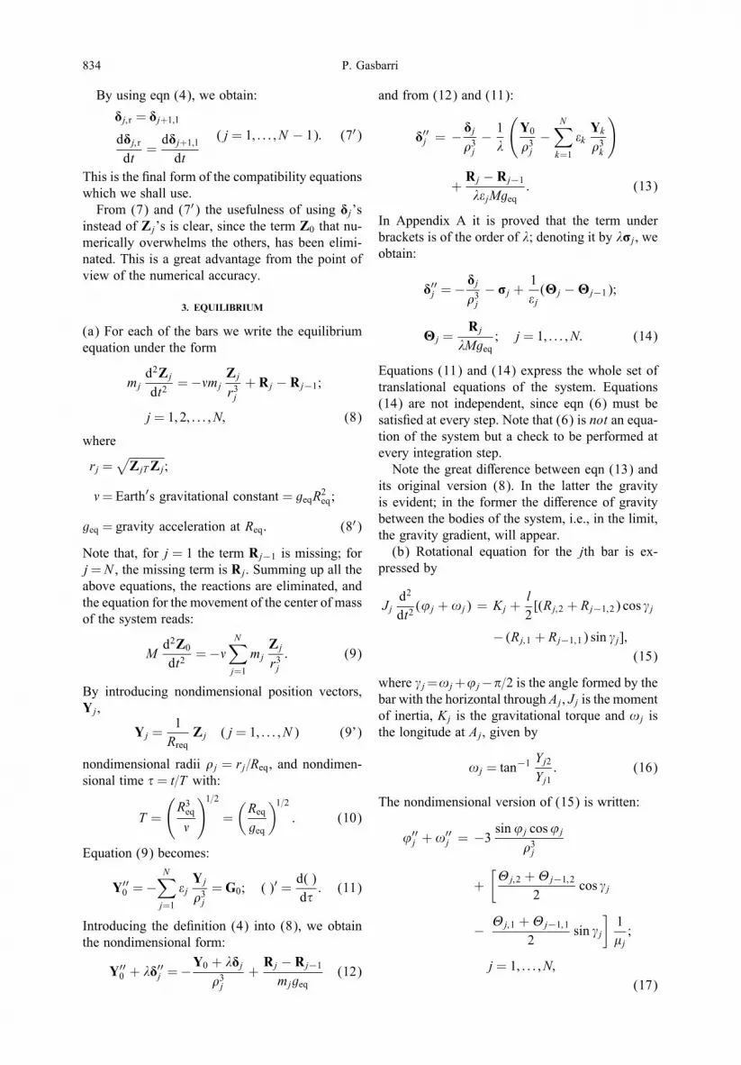
Fig. 5. Multibody conLgurations along 1st. orbit '=1:0,�= 1,(t = 0; �j = 0; j = 1; 5).

Fig. 6. Multibody conLgurations along 2nd. orbit '=1:0,�= 1,(t = 0; �j = 0; j = 1; 5).

positions, corresponding to even multiples of ’ =�=2 (stable) and odd multiples (unstable).Figures 5 and 6 provide the conLgurations as-

sumed by the multibody along the Lrst two orbits(note that due to graphical diSculties the scales ofthe bars and of the C.M (center of mass) orbit, arediDerent). As one can observe, since the initial con-Lguration of the bars corresponds to the unstableequilibrium position, after one orbit (counter clock-wise) their motion becomes unpredictable and twodiDerent kinds of motion can be distinguished; thefree rotation of the bars around their hinges and thecomplete rotation of the entire system around itscenter of gravity.


-0.2

-0.15

-0.1

-0.05

0

0.05

0.1

0.15

0.2

0.25

0.3

0 1 2 3 4 5

Rea

ctio

ns (

N)

(z1-

axis

)

ORBITS

Reaction Forces vs. Number of Orbits1234

Fig. 7. Reaction forces (Newton) vs. number of orbits(R1 components), ' = 1:0, �= 1.

-0.25

-0.2

-0.15

-0.1

-0.05

0

0.05

0.1

0.15

0.2

0 1 2 3 4 5

Rea

ctio

ns (

N)

(z2-

axis

)

ORBITS

Reaction Forces vs. Number of Orbits-1-2-3-4

Fig. 8. Reaction forces (Newton) vs. number of orbits(R2 components) ' = 1:0, �= 1.

Figures 7 and 8 provide the values of the reactionforces (R1 and R2 components, measured in New-tons) during the motion. Since only gravitationalforces are present in this example their values arevery small and of the order of magnitude of �Mgeq(see eqn (14)).Similar results are reported in Figs. 9–12 for the

case of �=0, (i.e., the bars have no initial angularvelocity). In this case the dynamic behavior of themultibody system (at least for the Lrst two orbits)is almost similar to that of a single bar orbitingaround the Earth, that was initially in an unstablestarting position.The eDect of the eccentricity ('=1:1) on the atti-

tude motion of the system was analyzed in Figs. 13and 14 (case �=0) and Figs. 15 and 16 (case �=1)for the “stable” initial conLgurations. From thesepictures it is possible to observe the well-knowneDect of orbital eccentricity, which could unstabi-lize the attitude motion of a spacecraft during itsorbital motion (as in this case).(b) All the previous examples refer to a chain

of bodies free to rotate around their hinges. In the

Fig. 9. Multibody conLgurations along 1st. orbit' = 1:0, �= 0,(t = 0; �j = 0; j = 1; 5).

Fig. 10. Multibody conLgurations along 2nd. orbit' = 1:0,�= 0,(t = 0; �j = 0; j = 1; 5).

following, it was considered the case of a system, inwhich, a rotatory motion to the end bar is imposedaccording to the law (Ref. [26]):

�(t) =

�0; t6 0;

�0 +U�16 [cos(

3�tUtm)− 9 cos( �t

Utm) + 8];

0¡t6Utm ;

�0 + U�; t¿Utm ;(28)

where �0 is the initial value of the angle of the bar,U� is the amplitude of the maneuver, and Utm isthe time of the maneuver. This kind of problem can

838 P. Gasbarri

-0.4

-0.3

-0.2

-0.1

0

0.1

0.2

0.3

0.4

0 1 2 3 4 5

Rea

ctio

ns (

N)

(z1-

axis

)

ORBITS


Fig. 11. Reaction forces (Newton) vs. number of orbits(R1 components), ' = 1:0, �= 0.

-0.4

-0.3

-0.2

-0.1

0

0.1

0.2

0.3

0.4

0 1 2 3 4 5

Rea

ctio

ns(N

) (z

2-ax

is)

ORBITS


Fig. 12. Reaction forces (Newton) vs. number of orbits(R2 components) ' = 1:0, �= 0.

Fig. 13. Multibody conLgurations along 1st. orbit' = 1:1, �= 0,(t = 0; �j = 80

◦; j = 1; 5).

Fig. 14. Multibody conLgurations along 2nd. orbit' = 1:1, �= 0,(t = 0; �j = 80

◦; j = 1; 5).

Fig. 15. Multibody conLgurations along 1st. orbit' = 1:1, �= 1,(t = 0; �j = 80

◦; j = 1; 5).

be considered as a typical inverse problem: giventhe motion of one or more bodies in the chain,determine the forces necessary to realize such amovement.The Lve bars here considered have the same

length (lj=10 m, j=1; : : : ; N ), the relevant massesand their initial angles are reported in Table 1.Fig. 17 shows the conLgurations assumed by the

multibody when a variation of angle U� = 45◦ inUtm = 60 s is imposed on the upper end bar of thechain. The required torque (in the Lrst 240 s) toperform the motion of the upper bar is sketched in


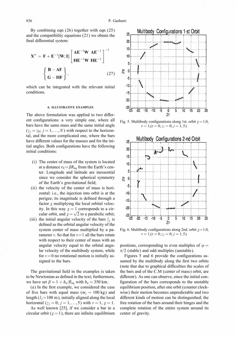
Fig. 16. Multibody conLgurations along 2nd. orbit' = 1:1, �= 1,(t = 0; �j = 80

◦; j = 1; 5).

Table 1. Multibody mass distribution and initial angles �j

Body 1 2 3 4 5

Mass (kg) 100 60 30 20 10Angle (deg) 60 65 70 75 80

Fig. 17. General layout:Multibody conLgurations along1st. orbits ' = 1:0.

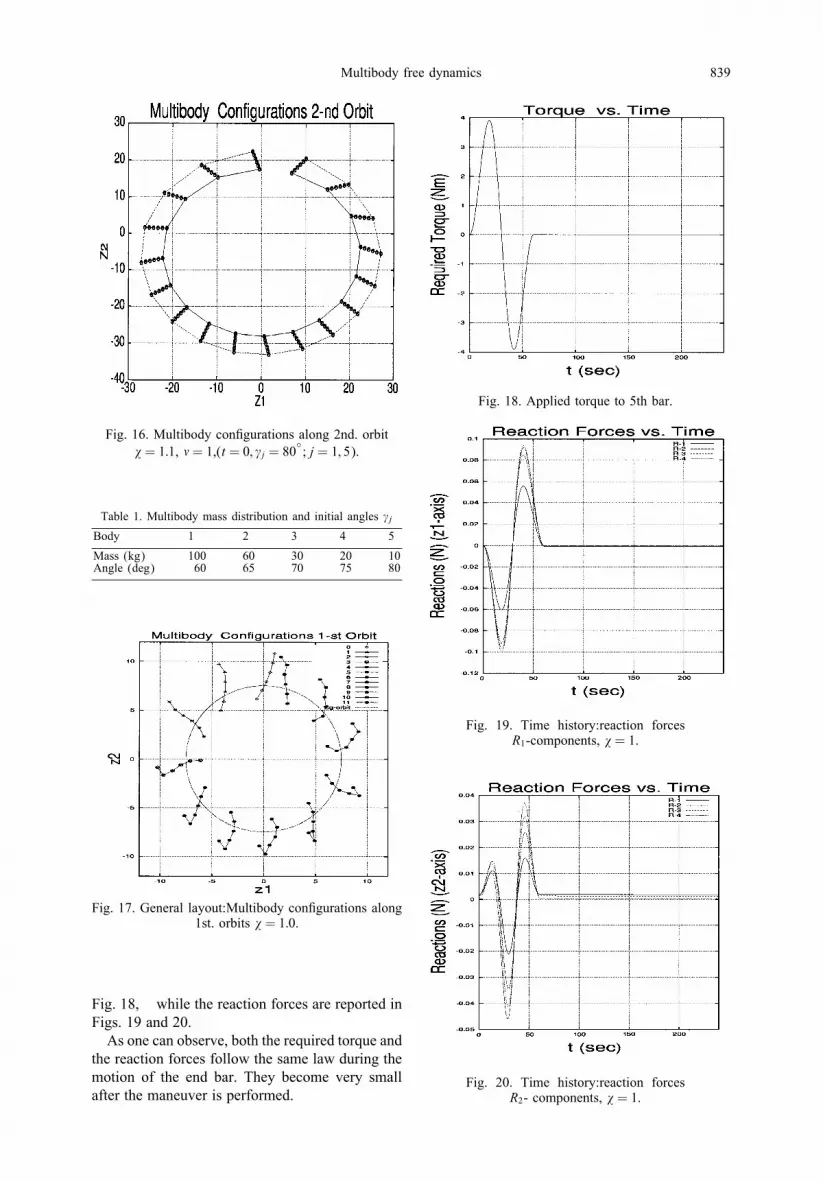
Fig. 18, while the reaction forces are reported inFigs. 19 and 20.As one can observe, both the required torque and

the reaction forces follow the same law during themotion of the end bar. They become very smallafter the maneuver is performed.

Fig. 18. Applied torque to 5th bar.

Fig. 19. Time history:reaction forcesR1-components, ' = 1.

Fig. 20. Time history:reaction forcesR2- components, ' = 1.

840 P. Gasbarri

7. CONCLUSIONS

The equation of motion of a multibody system ina space environment presented here, is based onthe Newtonian formulation rather than using an-alytic mechanics. An advantage provided by thisapproach is that the independent variables (e.g.,displacements and angular rotations of a singlebody) have straightforward physical meaning, giv-ing better insight into the dynamics. Secondly,possible control of multibody members could beachieved more easily using the degrees of freedomdeLned with the present approach rather than theLagrangian variables which are not necessarilysame as the former ones. Since the individual bodyparameters (position of its C.M, with respect to theinertial frame and rotation of the bar with respectto the inertial frame) are of diDerent order of mag-nitudes, they must be adequately separated. Thevector position of each body is given by specify-ing both the overall position of the system (of theorder of Earth’s radius), and the motion of eachbar relative to it (of the order of the member’sdimension). In doing this, the new motion param-eters are redundant and it is necessary therefore tointroduce reactions between the bodies as well asequations of compatibility.In order to account for the spherical gravitational

Leld of the Earth, the external forces considered inthe equations of motion, have been considered asa function of the positions of the bodies. As a con-sequence, no limitation on the size of the bodies isnecessary, and more accurate results are obtained.Another important aspect highlighted by this for-

mulation, is the introduction of a local (associatedto the motion of the C.M), as opposed to inertialreference frame. This is very important from a nu-merical point of view because, the coordinates ofthe bodies and the reaction forces under investi-gation are of the same order of magnitude in thatreference frame and therefore round-oD errors areavoided when evaluating them numerically.

Acknowledgements—The author acknowledges Prof.Santini’s constant guidance and support in this work.

REFERENCES

1. Meirovitch, L. and Lim, S., Maneuvering and controlof Nexible space robots. Journal of Guidance,Control and Dynamic 1994, 17 (3), 241–248.

2. De Silva, L. W., Trajectory design for roboticmanipulators in space applications. Journal ofGuidance, Control and Dynamic 1991, 14 (3),670–674.

3. Santini, P., Stability of Nexible spacecraft. ActaAstronautica 1976, 3, 687–713.

4. Meirovitch, L. and Chen, Y., Trajectory and controloptimization for Nexible space robots. Journal ofGuidance, Control and Dynamic 1995, 18 (3),493–502.

5. Meirovitch, L. and Kwak, M. K., Dynamicsand control of spacecraft with retargeting Nexibleantennas. Journal of Guidance, Control andDynamic 1990, 13 (2), 241–248.

6. Reyhanoglu, M. and Mc Glamroch, N., Planar re-orientation maneuvering of space multibody systemsusing internal controls. Journal of Guidance,Control and Dynamic 1992, 15 (6), 1475–1479.

7. Yamada, K., Attitude control of space robot by armmotion. Journal of Guidance, Control and Dynamic1997, 17 (5), 1050–1054.

8. Yamada, K. and Yoshikawa, S., Adaptive attitudecontrol for an artiLcial satellite with mobile bodies.Journal of Guidance, Control and Dynamic 1997,19 (4), 948–953.

9. Yamada, K. and Yoshikawa, S., Feedback control ofspace robot attitude by cyclic arm motion. Journalof Guidance, Control and Dynamic 1997, 20 (4),715–720.

10. Modi, V., No, A. C. and Karray, F., Slewingdynamics and control of the space station-basedmobile servicing system. Acta Astronautica 1995,35 (1=2), 119–129.

11. Schichlen, W. (ed.), Multibody System HandbookSpringer, Berlin, 1990.

12. Shabana, W. Dynamics of Multibody SystemsWiley, New York, 1989.

13. Ho, J. Y., Direct path method for Nexible multibodyspacecraft dynamics. Journal of Spacecraft andRockets 1977, 14, 102–110.

14. Kane, T. R. and Levinson, D. A., Formulation of theequation ofmotion for complex spacecraft. Journal ofGuidance,ControlandDynamic1980,3 (2),99–112.

15. Meirovitch, L. and Quinn, D., Equation of motionfor maneuvering Nexible spacecraft. Journal ofGuidance, Control and Dynamic 1987, 10 (2),453–465.

16. Modi, V. and Ibrahim, A. M., A general formulationfor librational dynamics of spacecraft with deployingappendages. Journal of Guidance, Control andDynamic 1984, 7, 563–569.

17. Santini, P., Betti, F., Gasbarri, P., Gaudenzi, P.,Persiani, F. and Saggiani, G. M., On possibleapplications of smart structure to control of spacesystems. Agard Conference Proceedings, SMP CP531, 1993, pp. 26.1–26.14.

18. Santini, P., Gasbarri, P., Betti, F. and Rossi, A.,Control of Nexible multi-body system by meansof intelligent structure. Dynamic and Control ofStructures in Space II, Computational MechanicsPublications, Southampton (Ed. C. L. Kirk, P. C.Hughes), 1993, pp. 585–602.

19. Gear, C. W. and Petzold, L. R., ODE methods forthe solution of diDerential=algebraic systems. SIAMJournalofNumericalAnalysis1984,21 (4)716–728.

20. Petzold, L. R. and Potra, F. A., ODAE methodsfor numerical solution of Euler–Lagrange equations.AppliedNumericalMathemarics1992,10, 397–413.

21. Potra, F. A., Implementation of linear multistepmethods for solving constrained equations ofmotions. SIAM, Journal of Numerical Analysis1993, 30 (3), 774–789.


22. Kirk, C. L. and Romero, I., Dynamic of a Nexibledeployable robotic manipulator. Dynamic andControl of Structures in Space III, ComputationalMechanics Publications (Ed. C. L. Kirk, D. J.Inman), 1996, pp 83–100.

23. Nelson, G. and Quinn, R., A quasi coordinateformulation for dynamic simulation of complexmultibody systems with constraints. Dynamic andControl of Structures in Space III, ComputationalMechanics Publications (Ed. C. L. Kirk, D. J.Inman), 1996, pp 523–538.

24. Krishnan, S. and Vadali, S. R., Near optimalthree dimensional maneuvers of spacecraft usingmanipulator arms. Journal of Guidance,Control andDynamic 1995, 18 (4), 932–943.

25. Santini, P., Gasbarri, P. and Benedetti, R., Motionof satellite in elliptic orbit. Complexity in Physicsand Technology, World ScientiLc, Singapore, 1992,pp. 91–109.

26. Violetti, A., Simulazione inversa delle manovre diun modello di elicottero. Master dissertation, 1998.

APPENDIX A.

We re-write the term within brackets of (13) as

�j =1�

N∑k=1

�kYk

(1�3j

− 1�3k

): (A.1)

Furthermore,(1�3j

− 1�3k

)= (�2k − �2j )fjk ;

fjk =�2j + �2k + �j�k

�3j �3k(�j + �k)

: (A.2)

Note that the calculation of fjk does not involve numer-ical eliminations.Now since,

�2k = Y0TY0 + 2�Y0TTk + �2TkTTk (A.3)

and a similar expression is valid for �j , we have:

�2k − �2j = �gjk ; (A.4)

where

gjk = 2Y0T (Tk − Tj) + �(TkTTk − TjTTj): (A.5)

Finally eqn (A.1) becomes:

�j =N∑

k=1

�kfjkgjkYk : (A.6)

APPENDIX B.

(a) The vector X contains all the unknowns of theproblem. It is ordered in blocks of three quantities,#j1; #j2; ’j , each corresponding to the jth bar, accord-ing to the following scheme (in transposed form to savespace)

XT

=[#11; #12; ’1︸︷︷︸block 1

| · · · | #j1; #j2; ’j︸︷︷︸block j

| · · · | Y01; Y02︸︷︷︸block N+1

]:

(B.1)

The last block is of two rows only; it includes the com-ponents of position vector of the center of mass.(b) The matrix E is diagonal

E = diag[�1; �1; !1; : : : ; �j ; �j ; !j; : : : ; �N ; �N ; !N ; 1; 1]:(B.2)

(c) The vector F is arranged like X. Consider theblock j; its two Lrst elements are:

qj1 =−#j1

�3j− ,j1;

qj2 =−#j2

�3j− ,j2: (B.3)

For the third row, we need to express !′′j . Now since

!j = tan−1 Yj2

Yj1; (B.4)

simple algebra leads to the expression:

!′′j = -j1#

′′j1 + -j2#

′′j2 + &j1Y

′′01 + &j2Y

′′02 + .j; (B.5)

where

&j1 =− Yj2

(Y 2j1 + Y 2j2)2; &j2 =

Yj1

(Y 2j1 + Y 2j2)2;

-j1 = �&j1; -j2 = �&j2;

.j =−2 (Yj1Y ′j1 + Yj2Y ′

j2)(Yj1Y ′j2 − Yj2Y ′

j1)(Y 2j1 + Y 2j2)2

:

(B.6)

Now we introduce the expressions already found; thethird row of block j of the vector F reads:

qj3 = −3 sin’j cos’j

�3j− -j1qj1 − -j2qj2

−&j1G01 − &j2G02 − .j; (B.7)

where, G01 and G02 are two components of the vectorG0, deLned in eqn (11).(d) The matrixW is partitioned into blocks, NX ×NR,

generally zero. Nonzero blocks are only N × (N − 1),each consisting of three rows and four columns.

j−1;1 j−1;2 j;1 j;2

#′′j1 −1 0 1 0#′′j2 0 −1 0 1’′′

j − sin �j2 + -j1

cos �j2 + -j2 − sin �j

2 − -j1cos �j2 − -j2

For the third row we have summed up the contribu-tions deriving from eqn (18) to those coming from eqn(B.7), respectively.

APPENDIX C.

Considering eqn (5), and deLne k=1 for (l) and k=2for (r); thus, for the end displacement of Bj , we have:

Tjk = Tj + (−1)(k) l2

[cos �j

sin �j

]; k = 1; 2: (C.1)

842 P. Gasbarri

DiDerentiating twice, and after some lengthy algebrawe obtain:

T′′jk = (C( jk)|T( jk))Dj + S( jk); (C.2)

where

DjT = {#′′j1; #′′j2; ’′′j1; Y

′′01; Y

′′02} (C.3)

and

C( jk)11 = 1− (−1)(k) 12 -j1 sin �j;

C( jk)12 =−(−1)(k) 12 -j2 sin �j;

C( jk)13 =−(−1)(k) 12 sin �j;

T ( jk)11 =−(−1)(k) 12 &j1 sin �j;

T ( jk)12 =−(−1)(k) 12 &j2 sin �j;

C( jk)21 = (−1)(k) 12 -j1 cos �j;

C( jk)22 = 1 + (−1)(k) 12 -j2 cos �j;

C( jk)23 = (−1)(k) 12 cos �j;

A =

−C(12) C(21) : : : : : : : : T(21) − T(12)

: : : : : : : : : : :

: : : : : : : : : : :

: : : : : : : : : : : :

: : : : : : : : : : : :

: : : : : : : : : : : :

: : : : : −C(j−1;2) C(j1) : : : : T(j1) − T(j−1;2)

: : : : : : : : : : : :

: : : : : : : : : : :

: : : : : : : : : : : :

: : : : : : : : : : : :

: : : : : : : : : : : :

: : : : : : : : : : : :

: : : : : : : : : −C(N−1;2) C(N1) T(N1) − T(N−1;2)

;

(C.8)

T ( jk)21 = (−1)(k) 12 &j1 cos �j;

T ( jk)22 = (−1)(k) 12 &j2 cos �j; (C.4)

S( jk)1 = (−1)(k)(− 12 (’

′j + !′

j)2 cos �j

− 12 -j1 sin �j);

S( jk)2 = (−1)(k)(− 12 (’

′j + !′

j)2 sin �j

− 12 -j1 cos �j); (C.5)

where

!′j =

Y ′j2Yj1 − Y ′

j1Yj2

(Y 2j1 + Y 2j2): (C.6)

Therefore the compatibility eqn (6) reads:

{[C( j−1;2)|T( j−1;2)]Dj−1 + S( j−1;2)

−[C( j;1)|T( j;1)]Dj − S( j;1)}= 0;

j = 2; : : : ; N (C.7)

and Lnally the matrices A and B of eqn (22) are assem-bled according the following scheme:

B =

S(21) − S(11)

::

S(j1) − S(j−1;1)

::

S(N1) − S(N−1;1)

: (C.9)

a two-dimensional approach to multibody free dynamics in space environment

Documents